frederick s. pardee center for international futures ... model v34.pdf · in reality, enrollment is...
TRANSCRIPT

1
FREDERICK S. PARDEE CENTER FOR INTERNATIONAL FUTURES
EXPLORE UNDERSTAND SHAPE
WORKING PAPER 2015.06.16
IFS EDUCATION MODEL DOCUMENTATION
Author: Mohammod T. Irfan
June 2017
Note: If cited or quoted, please indicate working paper status.
2
Table of Contents
1. Introduction............................................................................................................................................ 4
1.1 Conceptual Framework .................................................................................................................. 6
1.2 Dominant Relations: Education ..................................................................................................... 7
1.3 Key dynamics are directly linked to the dominant relations ......................................................... 8
1.4 Structure and Agent System: Education ........................................................................................ 8
2 Concepts and Coverage ....................................................................................................................... 10
2.1 National Education System .......................................................................................................... 10
2.2 Student Flow Rates ...................................................................................................................... 11
2.3 Attainment ................................................................................................................................... 11
2.4 Finance ......................................................................................................................................... 12
2.5 What the Model Does Not Cover ................................................................................................ 12
2.6 Variable Naming Convention ...................................................................................................... 12
3 Education Data ..................................................................................................................................... 12
3.1 Education Data Sources ............................................................................................................... 13
3.2 Processing Education Data in IFs ................................................................................................ 14
3.2.1 Model Initialization ............................................................................................................. 14
3.2.2 Data Reconciliation ............................................................................................................. 14
4 Education Flow Charts ........................................................................................................................ 15
4.1 Education Overview .................................................................................................................... 15
4.2 Education Student Flow ............................................................................................................... 16
4.3 Education Attainment .................................................................................................................. 18
4.4 Education Financial Flows .......................................................................................................... 21
5 Education Equations ............................................................................................................................ 23
5.1 Education Equations Overview ................................................................................................... 23
3
5.2 Education Equations: Student Flow: Regression Models for Core Flow Rates .......................... 24
5.3 Education Equations: Student Flow: Systemic Shift ................................................................... 26
5.4 Education Equations: Student Flow: Scenario Parameters .......................................................... 27
5.5 Primary Education: Grade Flow Algorithm ................................................................................ 27
5.5.1 Primary Education: Gross and Net Flow Rates ................................................................... 28
5.6 Education Equations: Secondary Education ................................................................................ 32
5.6.1 Lower Secondary Education: Grade Flow Algorithm ......................................................... 32
5.6.2 Lower Secondary Education: Key Relationships ................................................................ 34
5.6.3 Lower Secondary Education: Systemic Shift ...................................................................... 36
5.7 Upper Secondary Education ........................................................................................................ 37
5.8 Secondary Education: Vocational Education .............................................................................. 41
5.9 Secondary Education: Total Secondary ....................................................................................... 41
5.10 Education Equations: Tertiary ..................................................................................................... 42
5.10.1 Tertiary Education: Science and Technology Graduates ..................................................... 43
5.11 Education Equations: Budget Flow ............................................................................................. 44
5.11.1 Per Student Cost .................................................................................................................. 44
5.11.2 Budget Demand ................................................................................................................... 46
5.11.3 Budget Allocation Across Sectors of Spending ................................................................... 46
5.11.4 Budget Allocation Across Levels of Spending .................................................................... 48
5.11.5 Budget Impact on Enrollment .............................................................................................. 49
5.12 Education Equations: Attainment ................................................................................................ 50
5.12.1 Distribution by level of education completed ...................................................................... 50
5.12.2 Average Years of Education ................................................................................................ 51
5.12.3 Education Pyramids ............................................................................................................. 53
6 Knowledge Systems............................................................................................................................. 53
6.1 IFs Knowledge Indices: ............................................................................................................... 55
6.2 Knowledge Systems Equations: Total Knowledge Index ........................................................... 58
4
6.3 Knowledge Systems Equations: Knowledge Sub-Indices ........................................................... 59
7 Reference ............................................................................................................................................. 62
1. Introduction
Education is paramount to human and societal development. Yet many countries fail to provide
the opportunity of education for all citizen. What are the socio-economic consequences of
following this low-education path? How much resources do the societies require to sustain
and/or expand their educational participation and progression rates? What is the level of
educational attainment of the people in a society? How does that attainment impact the economic
and demographic outcomes in the society? What kind of resources are required to move
attainment? What is the payoff horizon of such attainment? Seeking interactive answers to such
education policy questions require a model that can study the dynamics of the education sector in
the broader context of economic activities, societal transitions and governance decisions.
International Futures (IFs) Model is an integrated global computer simulation attempting to
understand multiple cross-cutting issues areas including education and to explore possible
actions that can help countries change course. This document describes and explains the
International Futures education model.
IFs education model forecasts enrollment, financing and attainment of education in 186
countries. It covers formal education spanning elementary, lower secondary, upper secondary
and tertiary. It forecasts intake, survival, graduation and transition rates for each of these levels
separately for boys and girls. At the elementary level the model distinguishes between the of-age
and over-age pupils by computing a net rate and a gross rate for entrance and enrollment.
Secondary education is disaggregated in the model into lower and upper secondary each of
which are further divided into general and vocational programs. In addition to college graduates,
higher education model also computes science and engineering graduates. On the financial side,
the model compute total and per student spending at each level. Educational attainment variables
computed in the model are the level of education completed and the average years of education
acquired by the people grouped into five-year age-sex cohorts. The national education systems
simulated in the model follow UNESCO’s ISCED classification system of levels of education
and are thus roughly comparable even though the entrance ages or cycle lengths can slightly
differ among countries. The model runs recursively in annual time steps for a horizon that can be
extended to the end of the twenty first century.
The modeling methodology centers on a stock and flow accounting mechanism that tracks the
flow of children into, across and out of the stocks of pupils. The rates of flow are determined by
the secular trend of increasing education with increased level of development, the fiscal
constraints and the growth and saturation of rates as the economic and financial constraints are

5
lifted. As the boys and girls leave school they carry along the acquired education and the total
stock of attained education is adjusted accordingly.
The education model is developed as a sub-model of the International Futures (IFs) World
Model. Among the other IFs sub-models are - population, economy, government finance,
infrastructure, energy, health, governance and environment. Each of these models simulate the
complex interactions in one of the major human or natural systems and together they paint a
comprehensive picture of the key dynamics within and across these systems. The IFs models that
are most closely linked with the IFs education model are the demographic model, the economic
model and the model that represents government finance. The causal relationships simulated by
the models are often bi-directional, implemented through a combination of analytical functions,
table functions and various feedback algorithm. The example of such a bi-directional linkage is
the relationship between education and demography. On one hand, population of the
corresponding age groups, computed in the demographic model, are multiplied with student flow
rates to determine student headcount, on the other, education of women is one of the various
drivers of fertility rate. In a similar feedback relationship, additional investment in education,
assuming there is enough demand and no waste, would result in higher completion rates and
more educational attainment. The extra attainment would ultimately boost productivity, as the
better educated youth join the workforce, and make it possible to invest more in education.
IFs education model is not a novel attempt in building a global multi-country education
forecasting. Researchers have developed education models for projecting enrollment (Wils and
O’Connor 2003), costs (Delamonica, Mehrotra and Vandemoortele 2001; Bruns, Mingat and
Rakotomalala 2003), attainment (KC et al 2010) and impacts of education (McMahon 1999, KC
et al 2010). Most of these models project enrollment through trend extrapolation or a causal
relationship working directly on enrollment. In reality, enrollment is a stock that can change only
through inflows and/or outflows. IFs education model represents this stock and flow structure as
faithfully as possible by imposing the causal relationship only on the flow rates like entrance or
survival and computing enrollment through the accounting process. The flow rates themselves
are connected to the fundamentals in an endogenous model. The model tracks and connects the
educational efforts and attainment throughout the lifecycle of a person. The single-year age
cohorts computed in the IFs population model makes the simulation possible. Public financing of
education is integrated with the government budget process simulated in the IFs Government
finance model. The educational investment, in the model, brings in economic and social returns
at the national and the global level, explicitly or implicitly, as in the case of global impacts. At
the societal level, it attempts to simulate the interactions of education with the broader society in
an endogenous framework. The long run-horizon of the International Futures modeling platform
makes it possible for a model user to estimate the full returns of investment in education realized
over multiple generations. The model includes parameters, in all three areas - enrollment,
attainment and financing – making it possible to develop alternative scenarios to explore

6
uncertainties and to analyze policy interventions. The model thus serves as a generalized
thinking and analysis tool for educational futures within a broader human development context.
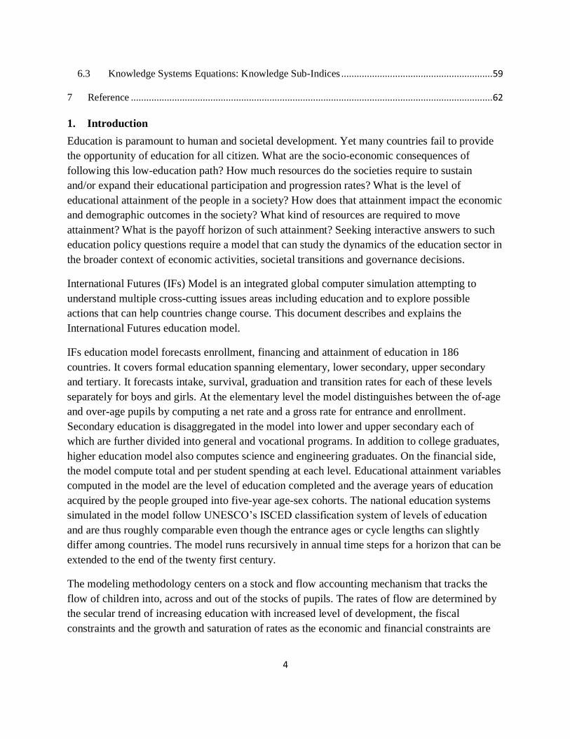
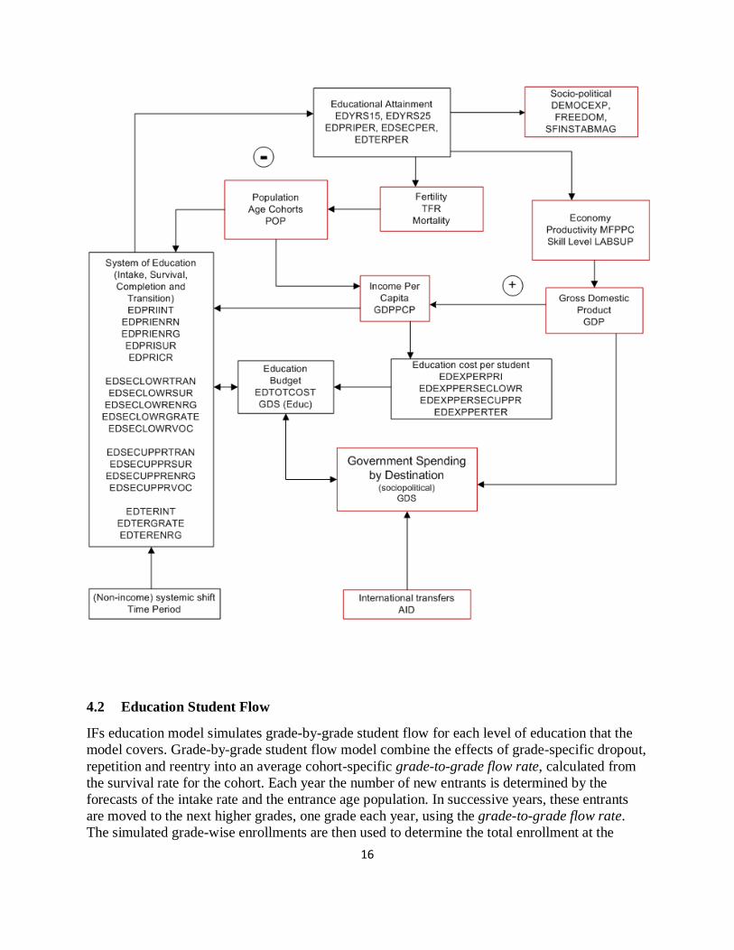
1.1 Conceptual Framework
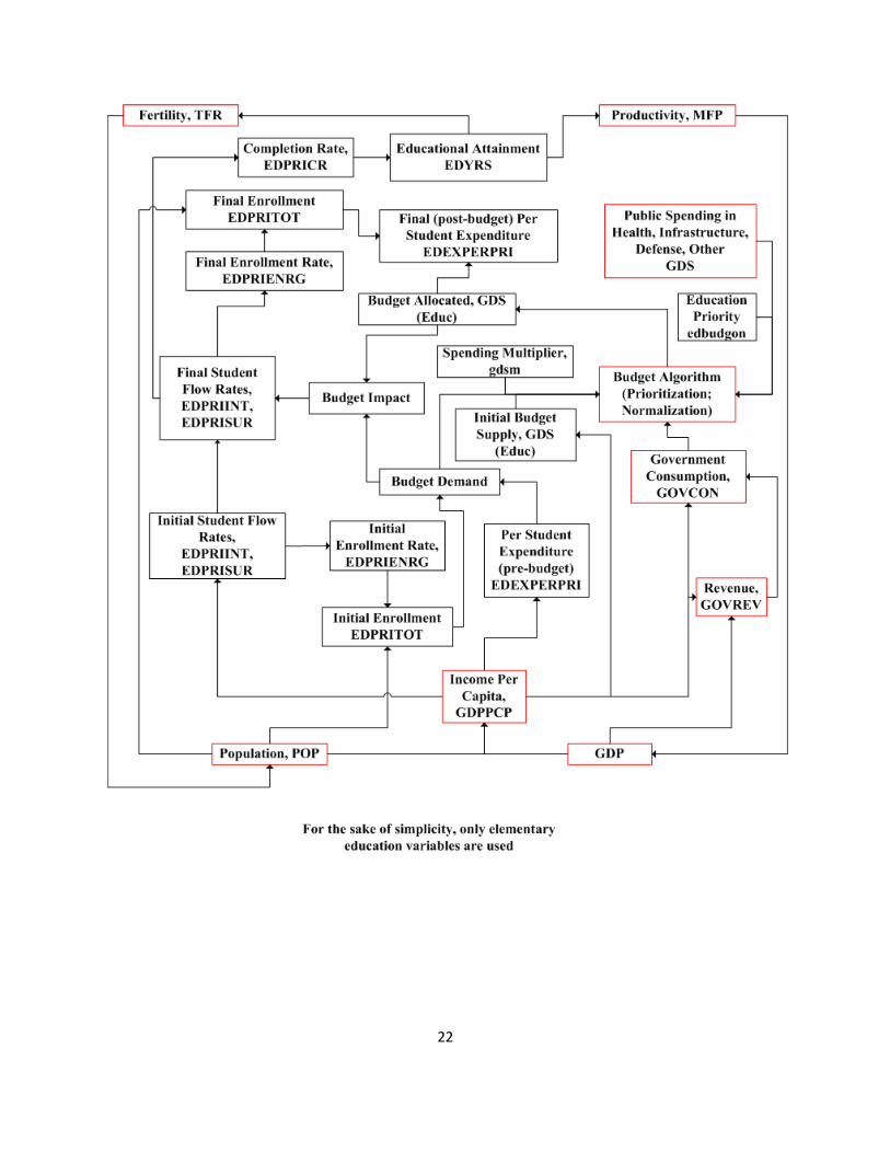
The next figure lays out the conceptual framework of the IFs education model. The figure shows:
a. Major algorithmic pieces inside the education module, e.g. student flows, budget
balancing
b. Other IFs models that drive or are driven by education variables, and
c. the causal connections with the direction of causation.
In the center of the figure we have the student flow and budget balancing piece, the core pieces
of our education model. On the two sides, we have Economy and Demography, the non-
educational models of highest relevance to education. Income per capita, widely used as an
indicator for the level of development of a society, computed in the Economy model of IFs
determine rates of entrance, persistence and transition. IFs cohort-specific demographic model
provides the school age population to the education model. The enrollment counts are obtained
by multiplying the population with the flow rates. These enrollments are multiplied with per
student cost, which is also driven by the level of income. The demand for funds is sent to the
government finance model. Domestic revenue and international transfers, computed in the
economic model, together form the total public funds available. The distribution of budget
among education and other public spending sectors takes place in the government finance model.
The stock of human capital (i.e., educational attainment of adults) gets updated in the model as
the children reach adulthood taking their educational accomplishment with them. Education of
people impact fertility, mortality and nutrition in the demographic and health models. In the IFs
model of economy, productivity is driven by human capital. Several variables in the IFs
governance model, for example state stability and democracy, also use education as a driver.
7
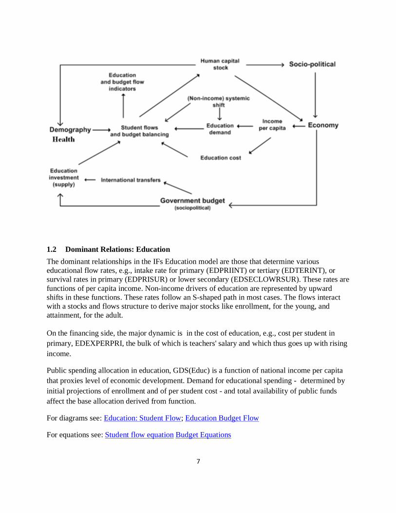
1.2 Dominant Relations: Education
The dominant relationships in the IFs Education model are those that determine various
educational flow rates, e.g., intake rate for primary (EDPRIINT) or tertiary (EDTERINT), or
survival rates in primary (EDPRISUR) or lower secondary (EDSECLOWRSUR). These rates are
functions of per capita income. Non-income drivers of education are represented by upward
shifts in these functions. These rates follow an S-shaped path in most cases. The flows interact
with a stocks and flows structure to derive major stocks like enrollment, for the young, and
attainment, for the adult.
On the financing side, the major dynamic is in the cost of education, e.g., cost per student in
primary, EDEXPERPRI, the bulk of which is teachers' salary and which thus goes up with rising
income.
Public spending allocation in education, GDS(Educ) is a function of national income per capita
that proxies level of economic development. Demand for educational spending - determined by
initial projections of enrollment and of per student cost - and total availability of public funds
affect the base allocation derived from function.
For diagrams see: Education: Student Flow; Education Budget Flow
For equations see: Student flow equation Budget Equations

8
1.3 Key dynamics are directly linked to the dominant relations
• Intake, survival and transition rates are functions of per capita income (GDPPCP). These
functions shift upward over time representing the non-income drivers of education.
• Each year flow rates are used to update major stocks like enrollment, for the young, and
attainment, for the adult.
• Per student expenditure at all levels of education is a function of per capita income.
• Deficit or surplus in public spending on education, GDS(Education), affects intake,
transition and survival rates at all levels of education.
1.4 Structure and Agent System: Education
Formal Education
System/Sub System Formal Education (elementary, lower
secondary, upper secondary and tertiary)
Organizing Structure Grade-flow model, i.e., entrance and
progression of children from one grade to the
next and transition from one level to the next.
Stocks Students, children
Flows Entrants, graduates, drop-outs
Key Aggregate Relationships Access, participation and progress rates move
with the level of development of the society.
Rates of change for the boys and girls
different with the boys gaining more access
and progression at the earlier levels. Rates
also vary by level of education. Higher levels,
understandably, move much slower than the
more basic levels.
Educational flow curves shift upward in the
long run as countries move towards a more
knowledge based society. The model
implements a systemic shift for some of the
curves.

9
Key Agent-Class Behavior Relationships Individuals and families decision to pursue
education
Education Finance
System/Sub System Government spending by destination
Organizing Structure Normalization of budget share given the
overall budget constraint and the emphasis on
education
Stocks Per student cost for different levels of
schooling
Flows Public spending in education
Key Aggregate Relationships Public spending available for education rises
with the growth in revenue collection that
moves with the level of development.
Cost of education rises with the income level
in the country.
Demand for public funds in education grows
with the growth in costs and/or the growth in
school-age population.
Education budget competes with other sectors
of government expenditure.
Enrollment and completion rates are affected
by funding decisions.
Educational budget push can affect other
development priorities.
Key Agent-Class Behavior Relationships Government revenue, expenditure and
transfer payment
Educational Attainment

10
System/Sub System Educational attainment of adults
Organizing Structure Distribution of population by age, sex and
educational attainment
Stocks Population, level and years of education
obtained
Flows Completion, drop-out, deaths, births, aging
Key Aggregate Relationships With the rise of enrollment and completion
attainment level change, first for the young
adults and, somewhat slowly, for the overall
population.
Key Agent-Class Behavior Relationships Higher level of attainments boosts economic
productivity.
Level of education of women affect fertility
rates.
2 Concepts and Coverage
2.1 National Education System
UNESCO has developed a standard classification system for national education systems called
International Standard Classification of Education (ISCED). ISCED 20111, which evolved from
the earlier ISCED 1997, uses a numbering system to identify the sequential levels of educational
systems—namely, pre-primary, primary, lower secondary, upper secondary, post-secondary non
tertiary and tertiary—which are characterized by curricula of increasing difficulty and
specialization as the students move up the levels. IFs education model covers primary (ISCED
level 1), lower secondary (ISCED level 2), upper secondary (ISCED level 3), and tertiary
education (ISCED levels 5A, 5B and 6).
The model covers 186 countries that can be grouped into any number of flexible country
groupings, e.g., UNESCO regions, like any other sub-module of IFs. Country specific entrance
age and school-cycle length data are collected and used in IFs to represent national education
systems as closely as possible. For all of these levels, IFs forecast variables representing student
flow rates, e.g., intake, persistence, completion and graduation, and stocks, e.g., enrolment, with
the girls and the boys handled separately within each country.
1 Please check http://uis.unesco.org/en/isced-mappings for more details on ISCED 2011 classification system

11
For lower and upper secondary, the IFs model covers both general and vocational curriculum and
forecasts the vocational share of total enrolment, EDSECLOWRVOC (for lower secondary) and
EDSECUPPRVOC (for upper secondary). Like all other participation variables, these two are
also disaggregated by gender. IFs model of tertiary education computes science and engineering
graduates, separately, in addition to all college graduates, higher education model
2.2 Student Flow Rates
Educational databases express flows of students through education systems as various rates of
flow, for example, intake rate or enrollment rate. These rates are not rates of change over time.
They are rather student shares of a relevant population group expressed as a percentage.
Depending on the particular rate of flow, the population used to compute the percentage share
could be:
- a single-year age-cohort, for example, number of new entrants in the first grade of
primary expressed as a percentage of population at the official entrance age of primary
gives the intake rate for primary (this is actually a net intake rate as opposed to a gross
rate, a distinction that we will explain soon). Intake and graduation rates at all levels use
single-year age cohort.
- a multi-year age cohort, for example, elementary enrollment rate is computed from the
number of primary pupils and the total population of the official age group corresponding
to the first to the final grade of primary. Enrollment rates need multi-year cohorts.
- a cohort of students, for example, survival rates in primary are computed as the
percentage of first graders who persist till the final grade of elementary. Another example
in this group is transition rate, which is expressed as a percentage of graduates in one
level who enter the first grade of the next level in a subsequent year.
Another important distinction among the flow rates is a gross rate versus a net rate, applicable to
some of the flows. The need for this distinction comes from the phenomenon of over-age (and in
some richer society cases, under-age) entrance and enrollment which could be substantial in low-
education countries in a catch up phase. Gross rates include all pupils or entrants, regardless of
age, whereas net rates include only those who are of the official age (or age group). All of the
flow rates forecast in the IFs education model are gross rates except three: entrance (or intake)
and enrollment rates in primary and enrollment rate in total secondary. This distinction does not
apply to survival or transition rates because of the way those variables are defined.
2.3 Attainment
The output of the national education system, i.e., school completion and partial completion of the
young people, is added to the educational attainment of the adults in the population. IFs forecasts
four categories of attainment - portion with no education, completed primary education,
completed secondary education and completed tertiary education - separately for men and
women above fifteen years of age by five year cohorts as well as an aggregate over all adult

12
cohorts. The model software contains so-called "Education Pyramid," a display of educational
attainments mapped over five-year age cohorts by sex as is usually done for population
pyramids.
Another aggregate measure of educational attainment that we forecast is the average years of
education of the adults. We have several measures, EDYEARSAG15, average years of education
for all adults aged 15 and above, EDYRSAG25, average years of education for those 25 and
older, EDYRSAG15TO24, average years of education for the youngest of the adults aged
between fifteen years to twenty-four.
2.4 Finance
IFs education model also covers financing of education. The model forecasts per student public
expenditure as a share of per capita income. The model also forecasts total public spending in
education and the share of that spending that goes to each level of education.
2.5 What the Model Does Not Cover
ISCED level 0, pre-primary, and level 4, post-secondary pre tertiary, are not common across all
countries and are thus excluded from the IFs education model which has a global coverage.
On the financing side, the model does not include private spending in education, a significant
share of spending especially for tertiary education in many countries and even for secondary
education in some countries. Scarcity of good data and lack of any pattern in the available data
precludes modelling private spending in education.
Quality of national education system can also vary across countries and over time. The IFs
education model does not forecast any explicit indicator of education quality. However, the
survival and graduation rates that the model forecasts for all levels of education are implicit
indicators of system quality. At this point IFs does not forecast any indicator of cognitive quality
of learners. However, the IFs database does have data on cognitive quality.
2.6 Variable Naming Convention
All education model variable names start with a two-letter prefix of 'ED' followed, in most cases,
by the three letter level indicator - PRI for primary, SEC for secondary, TER for tertiary.
Secondary is further subdivided into SECLOWR for lower secondary and SECUPPR for upper
secondary. Parameters in the model, which are named using lowercase letters like those in other
IFs modules, also follow a similar naming convention.
3 Education Data
An historical database plays an important role in the operationalization of a conceptual model.
The ongoing convergence of formal educational standards around the world made it easier for
international agencies and researchers to develop international educational standards and collect

13
comparable data with global coverage. This section describes how we have gathered and used
such data.
3.1 Education Data Sources
Data used in the IFs education model comes from international development agencies with
global or regional coverage, policy think-tanks and academic researchers. Some of these data are
collected through census and survey of educational institutes conducted by national governments
and reported to international agencies. Some data are collected through household surveys. In
some cases, data collected through survey and census are processed by experts to create
internationally comparable data sets.
UNESCO, the UN agency charged with collecting and maintaining education-related data from
across the world, is the primary source for the education data we use in the model. UNESCO
local offices collect the data by working with country governments. UNESCO Institute for
Statistics (UIS, http://uis.unesco.org/) publish global time series in their online data repository
whence we get the data.
World Bank’s World Development Indicator (WDI) database (http://data.worldbank.org/data-
catalog/world-development-indicators) incorporates major educational series from UIS. The
World Bank also maintains its own online educational database titled EdStats
(http://datatopics.worldbank.org/education/). EdStats has recently started adding data on
educational equality.
We would also like to mention some other international education database from which we do
not yet use any data in our model. UNICEF collects education data from households through
their Multiple Indicator Cluster Survey(MICS). Household level data is also collected by USAID
as a part of its Demographic and Household Surveys (DHS). Organization for Economic
Cooperation and Development (OECD), an intergovernmental organization of rich and
developed economies host an online education database at
http://www.oecd.org/education/database.htm. Their data covers thirty-five member countries and
some non-members (Argentina, Brazil, China, India Colombia, Costa Rica, Indonesia, Lithuania,
Russia, Saudi Arabia and South-Africa are some of the non-members covered in the OECD
database). OECD also publish an annual compilation of indicators titled Education at a Glance
(http://www.oecd.org/edu/education-at-a-glance-19991487.htm). OECD’s data include education
quality data in the form of internationally administered assessment tests. Several other regional
agencies, for example, Asian Development Bank or EU’s Eurostat also publish educational data
as a part of their larger statistical efforts.
Research organizations and academic researchers sometime compute education data not
available through survey and census, but can be computed from those. For example, the
educational attainment dataset compiled by Robert Barro and Jong Wha Lee (2013) is widely

14
used. International Institute for Applied Systems Analysis (IIASA) did also compile attainment
data using household survey data obtained from MICS and DHS surveys. Global Monitoring
Report team of UNESCO computes educational inequalities within and across countries and
publish them in a database titled World Inequality Database on Education
(http://www.education-inequalities.org/).
3.2 Processing Education Data in IFs
Enrollment, attainment and financing data that we collect from various sources are utilized in
two ways. First, data help us operationalize the dominant model relations by estimating the
direction, magnitude and strength of the relationship. Second, data is used for model
initialization as described in the next section.
3.2.1 Model Initialization
IFs education model, like all other IFs models, is a recursive dynamic model running in annual
time steps. Model initialization is handled in a preliminary process in which model variables are
assigned values for the starting year of the model’s run-horizon. The model pre-processor serves
two purposes. First, initialization with the most recent data ensures continuity between the real
world developments and the forecast. Second, inconsistency between historical data and model
equations are removed in the pre-processor through various reconciliation procedures.
3.2.2 Data Reconciliation
Inconsistencies among the base year primary flow rates (intake, survival, and enrollment) can
arise either from reported data values that, in combination, do not make sense, or from the use of
“stand-alone” cross-sectional estimations used in the IFs pre-Processor to fill missing data. Such
incongruities might arise among flow rates within a single level of education (e.g., primary
intake, survival, and enrollment rates that are incompatible) or between flow rates across two
levels of education (e.g., primary completion rate and lower secondary intake rate).
The IFs education model uses algorithms to reconcile incongruent flow values. They work by
(1) analyzing incongruities; (2) applying protocols that identify and retain the data or estimations
that are probably of higher quality; and (3) substituting recomputed values for the data or
estimations that are probably of lesser quality. For example, at the primary level, data on
enrollment rates are more extensive and more straight-forward than either intake or survival data;
in turn, intake rates have fewer missing values and are arguably more reliable measures than
survival rates. The IFs pre-processor reconciles student flow data for Primary by using an
algorithm that assumes enrollment numbers to be more reliable than the entrance data and
entrance data to be more reliable than survival data.

15
4 Education Flow Charts
4.1 Education Overview
For each country, the IFs education model represents a multilevel formal education system that
starts at primary and ends at tertiary. Student flows, i.e., entry into and progression through the
system are determined by forecasts on intake and persistence (or survival) rates superimposed on
the population of the corresponding age cohorts obtained from IFs population forecasts. Students
at all levels are disaggregated by gender. Secondary education is further divided into lower and
upper secondary, and then further into general and vocational according to the curricula that are
followed.
The model represents the dynamics in education financing through per student costs for each
level of education and a total public spending in education. Policy levers are available for
changing both spending and cost.
School completion (or dropout) in the education model is carried forward as the educational
attainment of the overall population. As a result, the education model forecasts population
structures by age, sex, and attained education, i.e., years and levels of completed education.
The major agents represented in the education system of the model are households,—represented
by the parents who decide which of their boys and girls will go to school—and governments that
direct resources into and across the educational system. The major flows within the model are
student and budgetary, while the major stock is that of educational attainment embedded in a
population. Other than the budgetary variables, all the flows and stocks are gender disaggregated.
The education model has forward and backward linkages with other parts of the IFs model.
During each year of simulation, the IFs cohort-specific demographic model provides the school
age population to the education model. In turn, the education model feeds its calculations of
education attainment to the population model’s determination of women’s fertility. Similarly,
the broader economic and socio-political systems provide funding for education, and levels of
educational attainment affect economic productivity and growth, and therefore also education
spending.
The figure below shows the major variables and components that directly determine education
demand, supply, and flows in the IFs system. The diagram attempts to emphasize on the inter-
connectedness of the education model components and their relationship to the broader human
development system.
16
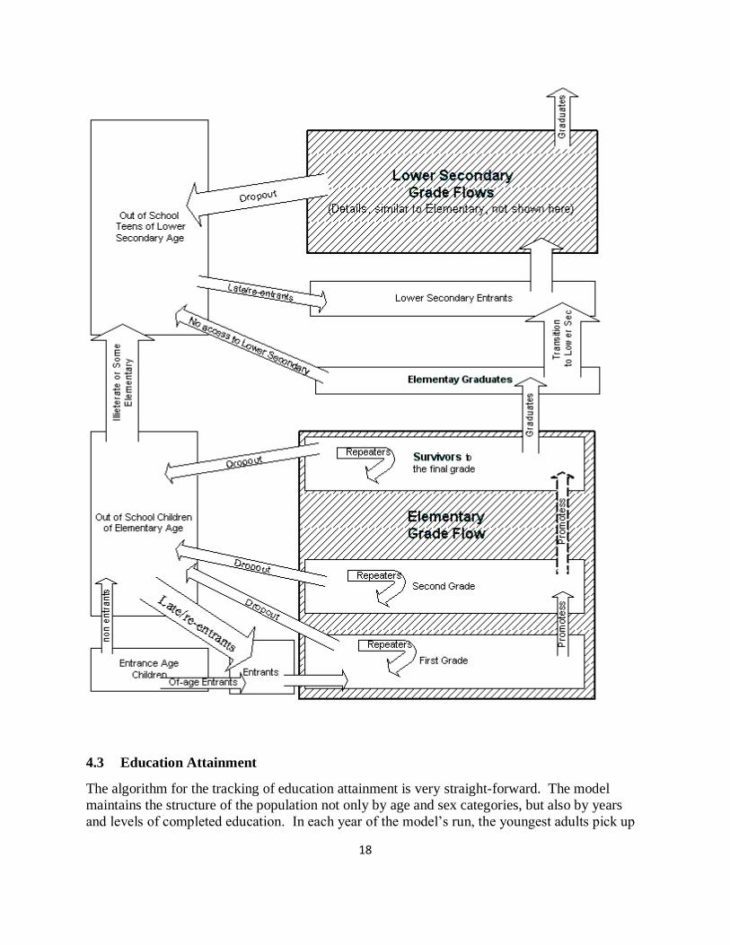
4.2 Education Student Flow
IFs education model simulates grade-by-grade student flow for each level of education that the
model covers. Grade-by-grade student flow model combine the effects of grade-specific dropout,
repetition and reentry into an average cohort-specific grade-to-grade flow rate, calculated from
the survival rate for the cohort. Each year the number of new entrants is determined by the
forecasts of the intake rate and the entrance age population. In successive years, these entrants
are moved to the next higher grades, one grade each year, using the grade-to-grade flow rate.
The simulated grade-wise enrollments are then used to determine the total enrollment at the

17
particular level of education. Student flow at a particular level of education, e.g., primary, is
culminated with rates of completion and transition by some to the next level, e.g., lower
secondary.
The figure below shows details of the student flow for primary (or, elementary) level. This is
illustrative of the student flow at other levels of education. We model both net and gross
enrollment rates for primary. The model tracks the pool of potential students who are above the
entrance age (as a result of never enrolling or of having dropped out), and brings back some of
those students, marked as late/reentrant in the figure, (dependent on initial conditions with
respect to gross versus net intake) for the dynamic calculation of total gross enrollments.
A generally similar grade-flow methodology models lower and upper secondary level student
flows. We use country-specific entrance ages and durations at each level. As the historical data
available does not allow estimating a rate of transition from upper secondary to tertiary, the
tertiary education model calculates a tertiary intake rate from tertiary enrollment and graduation
rate data using an algorithm which derives a tertiary intake with a lower bound slightly below the
upper secondary graduation rate in the previous year.
18
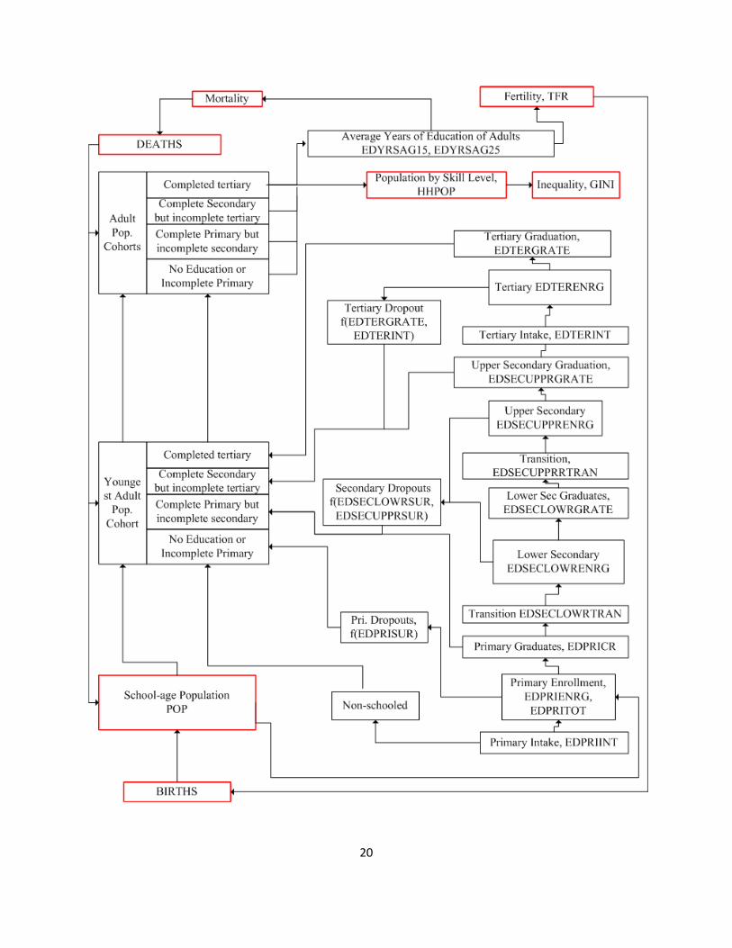
4.3 Education Attainment
The algorithm for the tracking of education attainment is very straight-forward. The model
maintains the structure of the population not only by age and sex categories, but also by years
and levels of completed education. In each year of the model’s run, the youngest adults pick up

19
the appropriate total years of education and specific levels of completed education. The model
advances each cohort in 1-year time steps after subtracting deaths. In addition to cohort
attainment, the model also calculates overall attainment of adults (15+ and 25+) as average years
of education (EDYRSAG15, EDYRSAG25) and as share of people 15+ with a certain level of
education completed (EDPRIPER, EDSECPER, EDTERPER).
One limitation of our model is that it does not represent differential mortality rates associated
with different levels of education attainment (generally lower for the more educated). 2 This
leads, other things equal, to a modest underestimate of adult education attainment, growing with
the length of the forecast horizon. The averaging method that IFs uses to advance adults through
the age/sex/education categories also slightly misrepresents the level of education attainment in
each 5-year category.
2 The multi-state demographic method developed and utilized by IIASA does include education-specific mortality
rates.
20
21
4.4 Education Financial Flows
In addition to student flows, and interacting closely with them, the IFs education model also
tracks financing of education. Because of the scarcity of private funding data, IFs specifically
represents public funding only, and our formulations of public funding implicitly assume that the
public/private funding mix will not change over time.
The accounting of educational finance is composed of two major components, per student cost
and the total number of projected students, the latter of the two is discussed in the student flows
section. Spending per student at all levels of education is driven by average income. Given
forecasts of spending per student by level of education and given initial enrollments forecasts by
level, an estimate of the total education funding demanded is obtained by summing across
education levels the products of spending per student and student numbers.
The funding needs are sent to the IFs government finance model where educational spending is
initially determined from the patterns in such spending regressed against the level of economic
development of the countries. A priority parameter (edbudgon) is then used to prioritize
spending needs over spending patterns. This parameter can be changed by model user within a
range of values going from zero to one with the zero value awarding maximum priority to fund
demands. Finally, total government consumption spending (GOVCON) is distributed among
education and other social spending sectors, namely infrastructure, health, public R&D, defense
and an "other" category, using a normalization algorithm.
Government spending is then taken back to the education module and compared against fund
needs. Budget impact, calculated as a ratio of the demanded and allocated funds, makes an
impact on the initial projection of student flow rates (intake, survival, and transition). The
positive (upward) side of the budget impact is non-linear with the maximum boost to growth
occurring when a flow rate is at or near its mid-point or within the range of the inflection points
of an assumed S-shaped path, to be precise. Impact of deficit is more or less linear except at
impact ratios close to 1, whence the downward impact is dampened. Final student flow rates are
used to calculate final enrollment numbers using population forecasts for relevant age cohorts.
Finally, cost per students are adjusted to reflect final enrollments and fund availability.
22

23
5 Education Equations
5.1 Education Equations Overview
The IFs education model represent two types of educational stocks, stocks of pupils and stocks of
adults with a certain level of educational attainment. These stocks are initialized with historical
data. The simulation model then recalculates the stock each year from its level the previous year
and the net annual change resulting from inflows and outflows.
The core dynamics of the model is in these flow rates. These flow rates are expressed as a
percentage of age-appropriate population and thus have a theoretical range of zero to one
hundred percent. Growing systems with a saturation point usually follow a sigmoid (S-shaped)
trajectory with low growth rates at the two ends as the system begins to expand and as it
approaches saturation. Maximum growth in such a system occurs at an inflection point, usually
at the middle of the range or slightly above it, at which growth rate reverses direction. Some
researchers (Clemens 2004; Wils and O’Connor 2003) have identified sigmoid trends in
educational expansion by analyzing enrollment rates at elementary and secondary level. The IFs
education model is not exactly a trend extrapolation; it is rather a forecast based on fundamental
drivers, for example, income level. Educational rates in our model are driven by income level, a
systemic shift algorithm and a budget impact resulting from the availability of public fund.
However, there are growth rate parameters for most of the flows that allow model user to
simulate desired growth that follows a sigmoid-trajectory. Another area that makes use of a
sigmoid growth rate algorithm is the boost in flow rates as a result of budget surplus.
Intake (or transition), survival, enrollment and completion are some of the rates that IFs model
forecast. Rate forecasts cover elementary, lower secondary, upper secondary and tertiary levels
of education with separate equations for boys and girls for each of the rate variables. All of these
rates are required to calculate pupil stocks while completion rate and dropout rate (reciprocal of
survival rate) are used to determine educational attainment of adults.
On the financial side of education, IFs forecast cost per student for each level. These per student
costs are multiplied with enrollments to calculate fund demand. Budget allocation calculated in
IFs socio-political module is sent back to education model to calculate final enrollments and cost
per student as a result of fund shortage or surplus.
The population module provides cohort population to the education model. The economic model
provides per capita income and the socio-political model provides budget allocation. Educational
attainment of adults calculated by the education module affects fertility and mortality in the
24
population and health modules, affects productivity in the economic module and affects other
socio-political outcomes like governance and democracy levels.
5.2 Education Equations: Student Flow: Regression Models for Core Flow Rates
Enrollments at various levels of education - EDPRIENRN, EPRIENRG, EDSECLOWENRG,
EDSECUPPRENRG, EDTERENRG - are initialized with historical data for the beginning year
of the model. Net change in enrollment at each time step is determined by inflows (intake or
transition) and outflows (dropout or completion). Entrance to the school system (EDPRIINT,
EDTERINT), transition from the lower level (EDSECLOWRTRAN, EDSECUPPRTRAN) - and
outflows - completion (EDPRICR), dropout or it's reciprocal, survival (EDPRISUR) - are some
of these rates that are forecast by the model.
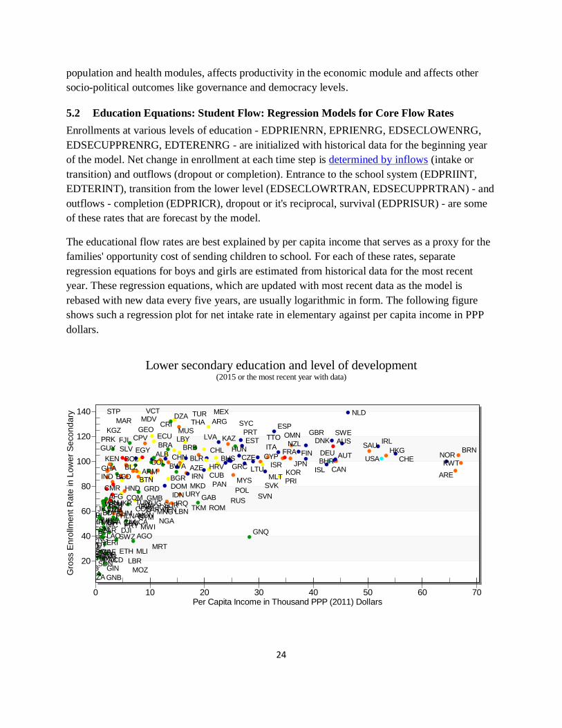
The educational flow rates are best explained by per capita income that serves as a proxy for the
families' opportunity cost of sending children to school. For each of these rates, separate
regression equations for boys and girls are estimated from historical data for the most recent
year. These regression equations, which are updated with most recent data as the model is
rebased with new data every five years, are usually logarithmic in form. The following figure
shows such a regression plot for net intake rate in elementary against per capita income in PPP
dollars.
AFG
ALB
DZA
AGO
ARG
ARM
AUS
AUT
AZE
BHS BHR
BGD
BRB
BLR
BLZ
BEN
BTN
BOL BWA
BRA BRN
BGR
BFA
BDI KHM
CMR
CAN
CPV
CAF TCD
CHL CHN
COL
COM
ZAR
COG
CRI
CIV
HRV
CUB
CYP CZE
DNK
DJI
DOM
ECU
EGY SLV
GNQ
ERI
EST
ETH
FJI
FIN FRA
GAB GMB
GEO
DEU
GHA GRC
GRD
GTM
GIN
GNB
GUY
HND
HKG HUN
ISL IND
IDN
IRN
IRQ
IRL
ISR
ITA
JAM
JPN
JOR
KAZ
KEN
PRK
KOR
KWT
KGZ
LAO
LVA
LBN
LSO
LBR
LBY
LTU
MKD
MDG
MWI
MYS
MDV
MLI
MLT
MRT
MUS
MEX
FSM MDA
MON MNG
MAR
MOZ
MMR
NAM NPL
NLD
NZL
NIC
NER
NGA
NOR
OMN
PAK
WBG
PAN
PNG
PRY
PER
PHL
POL
PRT
PRI
ROM RUS
RWA
WSM
STP
SAU
SEN
YUG
SYC
SLE
SVK
SVN
SLB
SOM
ZAF
ESP
LKA
LCA
VCT
SDN
SSD
SUR
SWZ
SWE
CHE
SYR
TJK
TZA
THA
TMP
TGO
TON
TTO
TUN
TUR
TKM
UGA
UKR
ARE
GBR
USA
URY
UZB
VUT
VEN VNM
YEM ZMB
ZWE
20
40
60
80
100
120
140
0 10 20 30 40 50 60 70
Lower secondary education and level of development(2015 or the most recent year with data)
Gro
ss E
nro
llme
nt
Ra
te in
Lo
we
r S
eco
nd
ary
Per Capita Income in Thousand PPP (2011) Dollars
25
In each of the forecast years, values of the educational flow rates are first determined from these
regression equations. Independent variables used in the regression equations are endogenous to
the IFS model. For example, per capita income, GDPPCP, forecast by the IFs economic model
drives many of the educational flow rates. The following equation3 shows the calculation of one
such student flow rate (CalEdPriInt) from the log model of net primary intake rate shown in the
earlier figure.
𝐶𝑎𝑙𝐸𝑑𝑃𝑟𝑖𝐼𝑛𝑡𝑝=𝑚𝑎𝑙𝑒,𝑟,𝑡 = 65.9207 + 7.3423 ln 𝐺𝐷𝑃𝑃𝐶𝑃𝑟,𝑡
Subscript p in the above equation (and all other equations in this document) stands for sex, r
stands for countries and t for time.
While all countries are expected to follow the regression curve in the long run, the residuals in
the base year make it difficult to generate a smooth path with a continuous transition from
historical data to regression estimation. We handle this by adjusting regression forecast for
country differences using an algorithm that we call "shift factor" algorithm. In the first year of
the model run we calculate a shift factor (EDPriIntNShift)as the difference (or ratio) between
historical data on net primary intake rate (EDPRIINTN) and regression prediction for the first
year for all countries. As the model runs in subsequent years, these shift factors (or initial ratios)
converge to zero or one if it is a ratio (an algorithmic procedure written as a code routine
ConvergeOverTime in the equation below) making the country forecast merge with the global
function gradually. The period of convergence for the shift factor (PriIntN_Shift_Time) is
determined through trial and error in each case.
𝐸𝑑𝑃𝑟𝑖𝐼𝑛𝑡𝑁𝑆ℎ𝑖𝑓𝑡𝑝,𝑟,𝑡=1 = 𝐸𝐷𝑃𝑅𝐼𝐼𝑁𝑇𝑁𝑝,𝑟,𝑡=1 − 𝐶𝑎𝑙𝐸𝑑𝑃𝑟𝑖𝐼𝑛𝑡𝑝,𝑟,𝑡=1
𝐸𝐷𝑃𝑅𝐼𝐼𝑁𝑇𝑁𝑝,𝑟,𝑡
= 𝐶𝑎𝑙𝐸𝑑𝑃𝑟𝑖𝐼𝑛𝑡𝑝,𝑟,𝑡
+ ConvergeOverTime(𝐸𝑑𝑃𝑟𝑖𝐼𝑛𝑡𝑁𝑆ℎ𝑖𝑓𝑡𝑝,𝑟,𝑡=1, 0, 𝑃𝑟𝑖𝐼𝑛𝑡𝑁_𝑆ℎ𝑖𝑓𝑡_𝑇𝑖𝑚𝑒)
The base forecast on flow rates resulting from these regression models are added with systemic
shift algorithm (see next section) and parameter impacts to calculate the initial or base flow rates.
These base flow rates might change as a result of budget impact based on the availability or
shortage of education budget explained in the budget flow section.
3 The name of the equation in the IFs table of functions is “GDP/Capita (PPP 2011) Versus Primary Net Intake Rate
Male (MostRecent) Log”
26
5.3 Education Equations: Student Flow: Systemic Shift
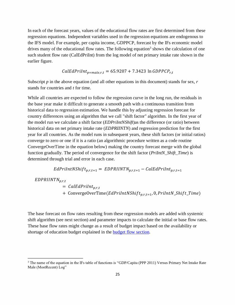
Access and participation in education increase with socio-economic developments that bring
changes to people's perception about the value of education. This upward shifts are clearly
visible in cross-sectional regression done over two adequately apart points in time. The next
figure illustrates such shift by plotting net intake rate for boys at the elementary level against
GDP per capita (PPP dollars) for two points in time, 1992 and 2000.
IFs education model introduces an algorithm to represent this shift in the regression functions.
This "systemic shift" algorithm starts with two regression functions about 10 to 15 years apart.
An additive factor to the flow rate is estimated each year by calculating the flow rate
(CalEdPriInt1 and CalEdPriInt2 in the equations below) progress required to shift from one
function, e.g., f1(𝐺𝐷𝑃𝑃𝐶𝑃𝑟,𝑡) to the other, f2(𝐺𝐷𝑃𝑃𝐶𝑃𝑟,𝑡), in a certain number of years
(SS_Denom), as shown below. This systemic shift factor (CalEdPriIntFac) is then added to the
flow rate (EDPRIINTN in this case) for a particular year (t) calculated from regression and
country shift as described in the previous section.
𝐶𝑎𝑙𝐸𝑑𝑃𝑟𝑖𝐼𝑛𝑡1𝑝,𝑟,𝑡 = f1(𝐺𝐷𝑃𝑃𝐶𝑃𝑟,𝑡)
𝐶𝑎𝑙𝐸𝑑𝑃𝑟𝑖𝐼𝑛𝑡2𝑝,𝑟,𝑡 = f2(𝐺𝐷𝑃𝑃𝐶𝑃𝑟,𝑡)
𝐶𝑎𝑙𝐸𝑑𝑃𝑟𝑖𝐼𝑛𝑡𝐹𝑎𝑐𝑝,𝑟,𝑡 =𝑡 − 1
𝑆𝑆_𝐷𝑒𝑛𝑜𝑚∗ (𝐶𝑎𝑙𝐸𝑑𝑃𝑟𝑖𝐼𝑛𝑡2𝑝,𝑟,𝑡 − 𝐶𝑎𝑙𝐸𝑑𝑃𝑟𝑖𝐼𝑛𝑡1𝑝,𝑟,𝑡)
𝐸𝐷𝑃𝑅𝐼𝐼𝑁𝑇𝑁𝑝,𝑟,𝑡 = 𝐸𝐷𝑃𝑅𝐼𝐼𝑁𝑇𝑁𝑝,𝑟,𝑡 + 𝐶𝑎𝑙𝐸𝑑𝑃𝑟𝑖𝐼𝑛𝑡𝐹𝑎𝑐𝑝,𝑟,𝑡

27
As said earlier, Student flow rates are expressed as a percentage of underlying stocks like the
number of school age children or number of pupils at a certain grade level. The flow-rate
dynamics work in conjunction with population dynamics (modeled inside IFs population
module) to forecast enrollment totals.
5.4 Education Equations: Student Flow: Scenario Parameters
Student flow rates calculated from the base model can be changed through parameters. Important
among the various parameters described in the scenario manual of the IFs system are multipliers,
annual growth parameters and target year parameters. These parameters will show their full
impact only when there is no or minimal budget constraint. The budget section of this document
and IFs scenario manual explains how one can prioritize education budget over other
government expenditure sections.
5.5 Primary Education: Grade Flow Algorithm
Once the core inflow (intake or transition) and outflow (survival or completion) are determined,
enrollment is calculated from grade-flows. Our grade-by-grade student flow model therefore uses
some simplifying assumptions in its calculations and forecasts. We combine the effects of grade-
specific dropout, repetition and reentry into an average cohort-specific grade-to-grade dropout
rate, calculated from the survival rate (EDPRISUR for primary) of the entering cohort over the
entire duration of the level (e.g., edprilen for primary). Each year the number of new entrants is
determined by the forecasts of the intake rate (EDPRIINT) and the entrance age population. In
successive years, these entrants are moved to the next higher grades, one grade each year,
subtracting the grade-to-grade dropout rate (DropoutRate). The simulated grade-wise
enrollments (GradeStudentsd,p,r,t where d is a subscript for the grade level) are then used to
determine the total gross enrollment at the particular level of education (EDPRIENRG for
Primary).
There are some obvious limitations of this simplified approach. While our model effectively
includes repeaters, we represent them implicitly (by including them in our grade progression)
rather than representing them explicitly as a separate category. Moreover, by setting first grade
enrollments to school entrants, we exclude repeating students from the first grade total. On the
other hand, the assumption of the same grade-to-grade flow rate across all grades might
somewhat over-state enrollment in a typical low-education country, where first grade drop-out
rates are typically higher than the drop-out rates in subsequent grades. Since our objective is to
forecast enrollment, attainment and associated costs by level rather than by grade, however, we
do not lose much information by accounting for the approximate number of school places
occupied by the cohorts as they proceed and focusing on accurate representation of total
enrollment.

28
𝐷𝑟𝑜𝑝𝑜𝑢𝑡𝑅𝑎𝑡𝑒p,r,t = 1 − (𝐸𝐷𝑃𝑅𝐼𝑆𝑈𝑅𝑝,𝑟,𝑡
100)
1𝐞𝐝𝐩𝐫𝐢𝐥𝐞𝐧𝐫−1
𝐺𝑟𝑎𝑑𝑒𝑆𝑡𝑢𝑑𝑒𝑛𝑡𝑠𝑑=1,𝑝,𝑟,𝑡 = 𝐸𝐷𝑃𝑅𝐼𝐼𝑁𝑇𝑝,𝑟,𝑡
𝐺𝑟𝑎𝑑𝑒𝑆𝑡𝑢𝑑𝑒𝑛𝑡𝑠𝑑,𝑝,𝑟,𝑡 = 𝐺𝑟𝑎𝑑𝑒𝑆𝑡𝑢𝑑𝑒𝑛𝑡𝑠𝑑−1,𝑝,𝑟,𝑡−1 ∗ (1 − 𝐷𝑟𝑜𝑝𝑜𝑢𝑡𝑅𝑎𝑡𝑒𝑝,𝑟,𝑡)
𝐸𝐷𝑃𝑅𝐼𝐸𝑁𝑅𝐺𝑝,𝑟,𝑡 = ∑ 𝐺𝑟𝑎𝑑𝑒𝑆𝑡𝑢𝑑𝑒𝑛𝑡𝑠𝑑,𝑝,𝑟,𝑡
𝒆𝒅𝒑𝒓𝒊𝒍𝒆𝒏𝒓
𝑑=1
5.5.1 Primary Education: Gross and Net Flow Rates
Student flow rates. defined as the percentage share of the children of appropriate-age who are in
the flow at a particular point in time, can be of two types depending on the age of the student.
For example, net enrollment rate in elementary counts only those students who are of
elementary-age while the gross elementary enrollment rate includes all pupils in primary
regardless of their age in the denominator for the computation of the rate. As the countries with
historically low rate of access to education approach a catch-up phase the difference between the
gross and the net rates of enrollment, entrance or graduation could be substantial in these
countries. Whether and how soon the gross-net gap narrow down in a society depends on the
ability and the efforts to expand access. In the current version of the model, we have a full grade-
flow model of both the gross enrollment and the net enrollment only for the level of elementary4.
The model starts with an initial estimation of the pool of out-of-school children for each of the
single year age-cohorts in a ten-year age-range starting at the entrance age of primary. These
children could either not attend school at all or had to drop out at some point. The estimation is
done by subtracting two numbers from the single-year cohort population (fagedst):
a. the age-specific enrollment, i.e., those of this single-year cohort who are in school, in an
age-appropriate or a higher grade, (Pristudentsbyage)
b. age-specific completion, i.e., those, of completion age or older, who have already
completed primary
4 We also have a net enrollment rate forecast for total secondary. That forecast is done through an
analytical function driven by the gross enrollment rate in the entire secondary, which is obtained
through a properly weighted average of enrollment rates in lower and upper secondary.
29
The first of these numbers, age-specific enrollment (PriStudentsbyAge) is computed by summing
up its two parts: those who are regular in entry and progression, and those who has become
irregular at some point. The number of regulars is obtained from the grade distribution of the net
enrollment (PristudentsNet). For the irregulars, we first calculate the number of overage in each
grade (OverAgeInTheGrade) and then distribute these overage across all single-year cohorts who
would be considered over-age for this grade. The distribution uses a normalization algorithm and
assumes that the current enrollment rates roughly mimic the age distribution of students. For
those who are above the completion age, the enrollment differential (deltaenr) between the final
and the penultimate grade is used to continue the distribution. As irregulars at all grades are
being distributed, the running total of age-specific enrollment rate is updated with the new
distribution.
𝑆ℎ𝑎𝑟𝑒𝑁𝑒𝑡 = 𝐸𝐷𝑃𝑅𝐼𝐸𝑁𝑅𝑁𝑝,𝑟,𝑡/𝐸𝐷𝑃𝑅𝐼𝐸𝑁𝑅𝐺𝑝,𝑟,𝑡
𝐷𝑒𝑙𝑡𝑎𝐸𝑛𝑟 = 𝑃𝑟𝑖𝑆𝑡𝑢𝑑𝑒𝑛𝑡𝑠𝑟,𝑑= 𝒆𝒅𝒑𝒓𝒊𝒍𝒆𝒏𝒓,𝑝,𝑡=1 − 𝑃𝑟𝑖𝑆𝑡𝑢𝑑𝑒𝑛𝑡𝑠𝑁𝑒𝑡𝑟,𝑑=𝒆𝒅𝒑𝒓𝒊𝒍𝒆𝒏𝒓−𝟏,𝑝,𝑡=1
𝑃𝑟𝑖𝑆𝑡𝑢𝑑𝑒𝑛𝑡𝑠𝑟,𝑑= 𝒆𝒅𝒑𝒓𝒊𝒍𝒆𝒏𝒓+𝟏,𝑝,𝑡 = 𝑓 (𝐷𝑒𝑙𝑡𝑎𝑅𝑛𝑟, 𝑆ℎ𝑎𝑟𝑒𝑁𝑒𝑡, 𝐸𝐷𝑃𝑅𝐼𝐶𝑅𝑝,𝑟,𝑡)
𝑇𝑜𝑡𝑂𝑣𝑒𝑟𝐴𝑔𝑒𝐸𝑛𝑅𝑎𝑡𝑒𝑇𝑜𝑡𝑑
= ∑ 𝑃𝑟𝑖𝑆𝑡𝑢𝑑𝑒𝑛𝑡𝑠𝑟,𝑑,𝑝,𝑡
𝒆𝒅𝒑𝒓𝒊𝒍𝒆𝒏𝒓
𝑑=𝑑+1
+ ∑ 𝑃𝑟𝑖𝑆𝑡𝑢𝑑𝑒𝑛𝑡𝑠𝑟,𝑑,𝑝,𝑡
𝟏𝟎
𝑑=𝒆𝒅𝒑𝒓𝒊𝒍𝒆𝒏𝒓+1
𝑂𝑣𝑒𝑟𝑎𝑔𝑒𝑆𝑡𝑢𝑑𝑒𝑛𝑡𝑠𝐼𝑛𝑡ℎ𝑒𝐺𝑟𝑎𝑑𝑒𝑟,𝑑,𝑝,𝑡=1
= 𝑃𝑟𝑖𝑆𝑡𝑢𝑑𝑒𝑛𝑡𝑠𝑟,𝑑 𝑝,𝑡=1 − 𝑃𝑟𝑖𝑆𝑡𝑢𝑑𝑒𝑛𝑡𝑠𝑁𝑒𝑡𝑟,𝑑,𝑝,𝑡=1
𝑃𝑟𝑖𝑆𝑡𝑢𝑑𝑒𝑛𝑡𝑠𝐵𝑦𝐴𝑔𝑒𝑟,𝑐=𝟏 𝑡𝑜 𝟏𝟎,𝑝,𝑡=1
= 𝑃𝑟𝑖𝑆𝑡𝑢𝑑𝑒𝑛𝑡𝑠𝑏𝑦𝐴𝑔𝑒𝑟,𝑐,𝑝,𝑡=1𝐶𝑎𝑙𝑐𝑢𝑙𝑎𝑡𝑒𝑑 𝑤𝑖𝑡ℎ 𝑑−1 + 𝑃𝑟𝑖𝑆𝑡𝑢𝑑𝑒𝑛𝑡𝑠𝑁𝑒𝑡𝑟,𝑑=𝒄,𝑝,𝑡=1
+ 𝑂𝑣𝑒𝑟𝑎𝑔𝑒𝑆𝑡𝑢𝑑𝑒𝑛𝑡𝑠𝐼𝑛𝑡ℎ𝑒𝐺𝑟𝑎𝑑𝑒𝑟,𝑑,=𝑐 𝑝,𝑡=1
∗ 𝑃𝑟𝑖𝑆𝑡𝑢𝑑𝑒𝑛𝑡𝑠𝑟,𝑑=𝑐,𝑝,𝑡
𝑇𝑜𝑡𝑂𝑣𝑒𝑟𝐴𝑔𝑒𝐸𝑛𝑅𝑎𝑡𝑒𝑇𝑜𝑡𝑑
Similarly, for completers, part b of the two part listed above, the of-age number of completers is
estimated from the gross completion rate (EDPRICR) and a ratio of the gross and net enrollment
30
rates (EDPRIENRN and EDPRIENRG). The rest of the elementary graduates are distributed
among those who are older than the completion age but younger enough to return to elementary.
Finally, the in-school (pristudentsbyage) and the completers (prigradbyage) are subtracted from
each of the ten single year cohorts to get the out-of-school children by single-year cohorts
(outofschoolbyage). Sum of these ten single-year cohorts give an estimate of the pool in the first
year of the model.
𝑜𝑢𝑡𝑜𝑓𝑠𝑐ℎ𝑜𝑜𝑙𝑏𝑦𝑎𝑔𝑒𝑟,𝑐=𝟏 𝑡𝑜 𝟏𝟎,𝑝,𝑡=1
= 𝑓𝑎𝑔𝑒𝑑𝑠𝑡𝑟,𝒆𝒅𝒑𝒓𝒊𝒔𝒕𝒂𝒓𝒕𝒓+𝑐−1,𝑝,𝑡=1 − 𝑃𝑟𝑖𝑆𝑡𝑢𝑑𝑒𝑛𝑡𝑠𝐵𝑦𝐴𝑔𝑒𝑟,𝑐,𝑝,𝑡=1
− 𝑃𝑟𝑖𝐺𝑟𝑎𝑑𝑠𝐵𝑦𝐴𝑔𝑒𝑟,𝑐,𝑝,𝑡=1
Once we have the number of children in the out-of-school pool, we can compute a rate of flow
from that pool to the first grade of primary (RetGr1Pcnt) using the initial year difference
between the gross and the net entrants as the numerator and the pool headcount as the
denominator.
𝑂𝑢𝑡𝑜𝑓𝑆𝑐ℎ𝑜𝑜𝑙𝑇𝑜𝑡 = ∑ 𝑜𝑢𝑡𝑜𝑓𝑠𝑐ℎ𝑜𝑜𝑙𝑏𝑦𝑎𝑔𝑒𝑟,𝑐,𝑝,𝑡=1
1 𝑡𝑜 10
𝑅𝑒𝑡𝐺𝑟1𝑃𝑐𝑛𝑡𝑟,,𝑝,𝑡=1
= 𝑓𝑎𝑔𝑒𝑑𝑠𝑡𝑟,𝒆𝒅𝒑𝒓𝒊𝒔𝒕𝒂𝒓𝒕𝒓,𝑝,𝑡=1 ∗ (𝑃𝑟𝑖𝑆𝑡𝑢𝑑𝑒𝑛𝑡𝑠𝑟,𝑑 𝑝,𝑡=1
− 𝑃𝑟𝑖𝑆𝑡𝑢𝑑𝑒𝑛𝑡𝑠𝑁𝑒𝑡𝑟,𝑑,𝑝,𝑡=1)/𝑜𝑢𝑡𝑜𝑓𝑠𝑐ℎ𝑜𝑜𝑙𝑇𝑜𝑡
In the subsequent years, the pool is updated from two outflows and two inflows: dropout from
schools in the previous year, entrant age children who could not enter school in the previous
year, late entry/return to schools in the current year and aging out of children who are no longer
young enough to try elementary education.
At first we advance the age of the age-specific out-of-school pool from the previous year. This
step takes care of aging out of the eldest cohort from the pool.
𝑜𝑢𝑡𝑜𝑓𝑠𝑐ℎ𝑜𝑜𝑙𝑏𝑦𝑎𝑔𝑒𝑟,𝑐= 2 𝑡𝑜 10,𝑝,𝑡 = 𝑜𝑢𝑡𝑜𝑓𝑠𝑐ℎ𝑜𝑜𝑙𝑏𝑦𝑎𝑔𝑒𝑟,𝑐−1,𝑝,𝑡−1
Then, we add those who missed entry as an inflow to the youngest cohort of the out-of-school
(outofschoolbyage r,1,p,t).
𝑜𝑢𝑡𝑜𝑓𝑠𝑐ℎ𝑜𝑜𝑙𝑏𝑦𝑎𝑔𝑒𝑟,1,𝑝,𝑡 = 𝑓𝑎𝑔𝑒𝑑𝑠𝑡𝑟,𝒆𝒅𝒑𝒓𝒊𝒔𝒕𝒂𝒓𝒕𝒓,𝑝,𝑡−1 ∗ (100 − 𝑃𝑟𝑖𝑆𝑡𝑢𝑑𝑒𝑛𝑡𝑠𝑁𝑒𝑡𝑟,1,𝑝,𝑡−1)/100
31
Next we compute the drop-outs of the previous year and then spread those drop-outs into single-
year age cohorts (Dropoutsfromspread r,c,p,t-1) using a similar normalization algorithm than we
have used in the first year to spread all over-age into age-specific cohorts.
𝑜𝑢𝑡𝑜𝑓𝑠𝑐ℎ𝑜𝑜𝑙𝑏𝑦𝑎𝑔𝑒𝑟,𝑐=2 𝑡𝑜 10 ,𝑝,𝑡 = 𝑜𝑢𝑡𝑜𝑓𝑠𝑐ℎ𝑜𝑜𝑙𝑏𝑦𝑎𝑔𝑒𝑟,𝑐,𝑝,𝑡 + 𝐷𝑟𝑜𝑝𝑜𝑢𝑡𝑠𝐹𝑟𝑜𝑚𝑆𝑝𝑟𝑒𝑎𝑑𝑟,𝑐,𝑝,𝑡−1
where
𝐷𝑟𝑜𝑝𝑜𝑢𝑡𝑠𝐹𝑟𝑜𝑚𝑆𝑝𝑟𝑒𝑎𝑑𝑟,𝑐,𝑝,𝑡−1
= f(𝑃𝑟𝑖𝑆𝑡𝑢𝑑𝑒𝑛𝑡𝑠𝑟,𝑑,𝑝,𝑡−1, 𝐷𝑟𝑜𝑝𝑜𝑢𝑡𝑠𝑟,𝑑,𝑝,𝑡−1, 𝑓𝑎𝑔𝑒𝑑𝑠𝑡𝑟,𝒄=𝒆𝒅𝒑𝒓𝒊𝒔𝒕𝒂𝒓𝒕𝒓+𝟏 𝒕𝒐 𝟏𝟎,𝑝,𝑡−1
The initial rate of return flow (RetGr1Pcnt) is converged gradually to 30% in 20 years, numbers
we obtained through trial and error, as the model proceeds to the subsequent years.
𝑅𝑒𝑡𝐺𝑟1𝑃𝑐𝑛𝑡𝑟,,𝑝,𝑡 = 𝐶𝑜𝑛𝑣𝑒𝑟𝑔𝑒𝑂𝑣𝑒𝑟𝑇𝑖𝑚𝑒(𝑅𝑒𝑡𝐺𝑟1𝑃𝑐𝑛𝑡𝑟,,𝑝,𝑡=1, .3,20)
Each year, the elementary entrants who are overage is computed by applying this rate of return to
each of the single-year cohorts in the out-of-school pool. The overage-entrant count is then
converted to a percentage of the cohort population (OverageinGr1Pcnt r, p, t).
𝑂𝑣𝑒𝑟𝐴𝑔𝑒𝑖𝑛𝐺𝑟1𝐶𝑜𝑢𝑛𝑡𝑟,𝑝,𝑡 = ∑ 𝑜𝑢𝑡𝑜𝑓𝑠𝑐ℎ𝑜𝑜𝑙𝑏𝑦𝑎𝑔𝑒𝑟,𝑐,𝑝,𝑡 ∗ 𝑅𝑒𝑡𝐺𝑟1𝑃𝑐𝑛𝑡𝑟,,𝑝,𝑡
1 𝑡𝑜 10
𝑂𝑣𝑒𝑟𝐴𝑔𝑒𝑖𝑛𝐺𝑟1𝑃𝑐𝑛𝑡𝑟,𝑝,𝑡 = 100 ∗ 𝑂𝑣𝑒𝑟𝐴𝑔𝑒𝑖𝑛𝐺𝑟1𝐶𝑜𝑢𝑛𝑡𝑟,𝑝,𝑡/𝑓𝑎𝑔𝑒𝑑𝑠𝑡𝑟,𝒄=𝒆𝒅𝒑𝒓𝒊𝒔𝒕𝒂𝒓𝒕𝒓,𝑝,𝑡
These over-age entrants are subtracted from each of the single-year cohorts of out-of-school
children in the pool.
𝑜𝑢𝑡𝑜𝑓𝑠𝑐ℎ𝑜𝑜𝑙𝑏𝑦𝑎𝑔𝑒𝑟,𝑐,𝑝,𝑡
= 𝑜𝑢𝑡𝑜𝑓𝑠𝑐ℎ𝑜𝑜𝑙𝑏𝑦𝑎𝑔𝑒𝑟,𝑐,𝑝,𝑡 − 𝑜𝑢𝑡𝑜𝑓𝑠𝑐ℎ𝑜𝑜𝑙𝑏𝑦𝑎𝑔𝑒𝑟,𝑐,𝑝,𝑡 ∗ 𝑅𝑒𝑡𝐺𝑟1𝑃𝑐𝑛𝑡𝑟,,𝑝,𝑡
Grade-flow for Gross Enrollment
The overage entrants computed as a percentage of the entrance age population
(OverageinGr1Pcnt r, p, t) computed in the pool algorithm is added to the net entrance rate
(EDPRIINTN r, p, t ) to obtain a gross entrance rate.
𝐸𝐷𝑃𝑅𝐼𝐼𝑁𝑇𝑝,𝑟,𝑡 = 𝐸𝐷𝑃𝑅𝐼𝐼𝑁𝑇𝑁𝑝,𝑟,𝑡 + 𝑂𝑣𝑒𝑟𝐴𝑔𝑒𝑖𝑛𝐺𝑟1𝑃𝑐𝑛𝑡𝑟,𝑝,𝑡
This gross entrance rate, the survival rate forecast and the number of students in each grade from
the previous years are later used to construct the grade-flow for all students. Please see the
section on primary education grade flow for further detail on this algorithm.

32
5.6 Education Equations: Secondary Education
Secondary education is further divided into two levels: a “lower secondary” level with
curriculum contents intended to enhance the basic skills obtained in primary and an upper
secondary education which is meant to prepare students for college. Both of these levels are three
years long, for most countries5. Many countries start classifying the students into a general
curriculum and a vocational6 track as soon as they start junior high. IFs education model
simulates the lower and upper secondary education of each of the model countries by laying out
a system that represents the country specific situation. For example, the cycle lengths for lower
(edseclowrlen) and upper secondary (edsecupprlen) have country specific values initialized with
data. Whether a country has vocational education or not and whether the vocational-general split
starts at lower secondary or upper, are also modeled according to the nature of the existing
system in the country. Since, lower and upper secondary has a very similar algorithm we
document below only one of these two levels, i.e., lower secondary and mention the differences
between the two levels, when there is any.
5.6.1 Lower Secondary Education: Grade Flow Algorithm
Like elementary, enrollment is the major stock in lower secondary. This stock change through a
grade-flow algorithm, again, similar to elementary. Lower secondary students are distributed into
the grades of lower secondary as the model starts. In subsequent model time steps, the flows that
affect the grade enrollments are:
- an inflow of children who complete primary and transition into the first grade of lower
secondary
- dropping out of some of the students from various grades of lower-secondary
- graduation from lower secondary
The table below lists the model variables at the cycle level that represent or determine these
stocks and flows.
Variable Definition Use
EDSECLOWRENRG Gross enrollment rate in
lower secondary
Stock variable expressed as the rate of
participation defined as total students in
lower secondary as a percentage share of
5 117 of the 186 IFs countries have a three-year lower secondary. Most of the remaining countries have a 4 year
lower secondary. Few countries, for example, Germany and Austria, have a unusually long lower secondary cycle of
six years. These countries have a shorter elementary cycle, thus keeping the pre-college year total at twelve or
thirteen. The number of three-year upper secondary countries is more than 140.
6 Technical and vocational education track or TVET is the term that UNESCO use

33
Variable Definition Use
total population in the lower-secondary-
age-group
EDSECLOWRTRAN
Rate of transition from
primary to lower
secondary7
This variable determines the inflow to
the first grade of lower secondary
EDSECLOWRGRATE Graduation rate at the
lower secondary level
Used in computing the drop-outs and the
graduates
Computation of the grade enrollment rates and the total enrollment is shown below. Subscript
notation used in these equations have the same meaning as in the other parts of this document (p
is for sex, r for country or region, t for time and d for grade, Ages for single-year age cohorts).
Intake into the first grade of lower secondary (caledsecint) is computed from enrollment rate in
the final grade of primary (pristudents) and the transition rate into lower secondary
(EDSECLOWRTRAN) as shown in the first equation. The next equation shows the computation
of total cycle drop-outs for this cohort of entrants. The assumptions for this computation is that
each of the grades will have the same rate of dropout (DropoutRate) and the rate of persistence
for the cohort is (roughly) equal to the ratio of the rate of entrance to the rate of graduation
(EDSECLOWRGRATE). Enrollment rates for the second and higher grades of lower secondary
are obtained from the rate of enrollment of the grade below in the year before and the rate of
grade drop-out. In a final step, the grade-wise enrollment rates (seclowrstudents) are multiplied
with population of the relevant cohort (fagedstc, where c is the subscript for cohort number) to
obtain headcount of students by grade. Grade headcounts are summed to total enrollment in
lower secondary (EDSECLOWRTOT). The headcount is divided by total number of boys or girls
of lower-secondary age-group (seclowrpop) and multiplied by one hundred to obtain the
enrollment rate.
𝑐𝑎𝑙𝑒𝑑𝑠𝑒𝑐𝑖𝑛𝑡𝑝,𝑟,𝑡 = 𝑝𝑟𝑖𝑠𝑡𝑢𝑑𝑒𝑛𝑡𝑠𝑒𝑑𝑝𝑟𝑖𝑙𝑒𝑛𝑟,𝑟,𝑡−1 ∗ 𝐸𝐷𝑆𝐸𝐶𝐿𝑂𝑊𝑅𝑇𝑅𝐴𝑁𝑝,𝑟,𝑡
𝐷𝑟𝑜𝑝𝑜𝑢𝑡𝑅𝑎𝑡𝑒𝑝,𝑟,𝑡 = 1 − (𝐸𝐷𝑆𝐸𝐶𝐿𝑂𝑊𝑅𝐺𝑅𝐴𝑇𝐸𝑝,𝑟,𝑡
𝑐𝑎𝑙𝑒𝑑𝑠𝑒𝑐𝑖𝑛𝑡𝑝,𝑟,𝑡)
1𝒆𝒅𝒔𝒆𝒄𝒍𝒐𝒘𝒓𝒍𝒆𝒏𝑟−1
7 Number of new entrants to the first grade of lower secondary expressed as a percentage of the
students enrolled in the last grade of primary in the previous year
34
𝑠𝑒𝑐𝑙𝑜𝑤𝑟𝑠𝑡𝑢𝑑𝑒𝑛𝑡𝑠𝐷=1,𝑝,𝑟,𝑡 = 𝑐𝑎𝑙𝑒𝑑𝑠𝑒𝑐𝑖𝑛𝑡𝑝,𝑟,𝑡
𝑠𝑒𝑐𝑙𝑜𝑤𝑟𝑠𝑡𝑢𝑑𝑒𝑛𝑡𝑠𝐷,𝑝,𝑟,𝑡 = 𝑠𝑒𝑐𝑙𝑜𝑤𝑟𝑠𝑡𝑢𝑑𝑒𝑛𝑡𝑠𝐷−1,𝑝,𝑟,𝑡−1 ∗ (1 − 𝐷𝑟𝑜𝑝𝑜𝑢𝑡𝑅𝑎𝑡𝑒𝑝,𝑟,𝑡)
𝑒𝑑𝑠𝑒𝑐𝑙𝑜𝑤𝑟𝑝𝑜𝑝𝑝,𝑟,𝑡 = ∑ 𝑓𝑎𝑔𝑒𝑑𝑠𝑡𝑐,𝑝,𝑟,𝑡
𝒆𝒅𝒑𝒓𝒊𝒔𝒕𝒂𝒓𝒕𝑟+ 𝒆𝒅𝒑𝒓𝒊𝒍𝒆𝒏𝑟+𝒆𝒅𝒔𝒆𝒄𝒍𝒐𝒘𝒓𝒍𝒆𝒏𝑟
𝑐 = 𝒆𝒅𝒑𝒓𝒊𝒔𝒕𝒂𝒓𝒕𝑟+ 𝒆𝒅𝒑𝒓𝒊𝒍𝒆𝒏𝑟
𝐸𝐷𝑆𝐸𝐶𝐿𝑂𝑊𝑅𝑇𝑂𝑇𝑝,𝑟,𝑡
= ∑ ( 𝑠𝑒𝑐𝑙𝑜𝑤𝑟𝑠𝑡𝑢𝑑𝑒𝑛𝑡𝑠𝑑,𝑝,𝑟,𝑡
𝒆𝒅𝒔𝒆𝒄𝒍𝒐𝒘𝒓𝒍𝒆𝒏𝑟
𝑑=1
∗ 𝑓𝑎𝑔𝑒𝑑𝑠𝑡 𝑑+ 𝑒𝑑𝑝𝑟𝑖𝑠𝑡𝑎𝑟𝑡𝑟+ 𝑒𝑑𝑝𝑟𝑖𝑙𝑒𝑛𝑟 ,𝑝,𝑟,𝑡)
𝐸𝐷𝑆𝐸𝐶𝐿𝑂𝑊𝑅𝐸𝑁𝑅𝐺𝑝,𝑟,𝑡 = 100 ∗ 𝐸𝐷𝑆𝐸𝐶𝐿𝑂𝑊𝑅𝑇𝑂𝑇𝑝,𝑟,𝑡 / 𝑒𝑑𝑠𝑒𝑐𝑙𝑜𝑤𝑟𝑝𝑜𝑝𝑝,𝑟,𝑡
5.6.2 Lower Secondary Education: Key Relationships
Rates of transition into lower secondary (EDSECLOWRTRAN) and rates of graduation from
lower secondary are driven in the IFs education model by per capita income indicating the level
of development of the country and the ability and aspiration of the families. For each of these
rates, separate regression equations for boys and girls are estimated from historical data for the
most recent year. The regression equations, drawn with most recent historical data, are all
logarithmic. The figure below shows the logarithmic functions for the transition rates for the
boys and the girls.
35
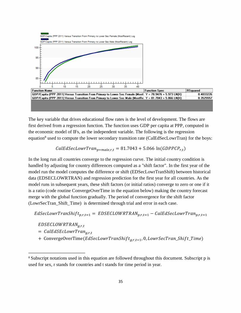
The key variable that drives educational flow rates is the level of development. The flows are
first derived from a regression function. The function uses GDP per capita at PPP, computed in
the economic model of IFs, as the independent variable. The following is the regression
equation8 used to compute the lower secondary transition rate (CalEdSecLowrTran) for the boys:
𝐶𝑎𝑙𝐸𝑑𝑆𝑒𝑐𝐿𝑜𝑤𝑟𝑇𝑟𝑎𝑛𝑝=𝑚𝑎𝑙𝑒,𝑟,𝑡 = 81.7043 + 5.066 ln(𝐺𝐷𝑃𝑃𝐶𝑃𝑟,𝑡)
In the long run all countries converge to the regression curve. The initial country condition is
handled by adjusting for country differences computed as a "shift factor". In the first year of the
model run the model computes the difference or shift (EDSecLowrTranShift) between historical
data (EDSECLOWRTRAN) and regression prediction for the first year for all countries. As the
model runs in subsequent years, these shift factors (or initial ratios) converge to zero or one if it
is a ratio (code routine ConvergeOverTime in the equation below) making the country forecast
merge with the global function gradually. The period of convergence for the shift factor
(LowrSecTran_Shift_Time) is determined through trial and error in each case.
𝐸𝑑𝑆𝑒𝑐𝐿𝑜𝑤𝑟𝑇𝑟𝑎𝑛𝑆ℎ𝑖𝑓𝑡𝑝,𝑟,𝑡=1 = 𝐸𝐷𝑆𝐸𝐶𝐿𝑂𝑊𝑅𝑇𝑅𝐴𝑁𝑝,𝑟,𝑡=1 − 𝐶𝑎𝑙𝐸𝑑𝑆𝑒𝑐𝐿𝑜𝑤𝑟𝑇𝑟𝑎𝑛𝑝,𝑟,𝑡=1
𝐸𝐷𝑆𝐸𝐶𝐿𝑂𝑊𝑅𝑇𝑅𝐴𝑁𝑔,𝑟,𝑡
= 𝐶𝑎𝑙𝐸𝑑𝑆𝐸𝑐𝐿𝑜𝑤𝑟𝑇𝑟𝑎𝑛𝑔,𝑟,𝑡
+ ConvergeOverTime(𝐸𝑑𝑆𝑒𝑐𝐿𝑜𝑤𝑟𝑇𝑟𝑎𝑛𝑆ℎ𝑖𝑓𝑡𝑔,𝑟,𝑡=1, 0, 𝐿𝑜𝑤𝑟𝑆𝑒𝑐𝑇𝑟𝑎𝑛_𝑆ℎ𝑖𝑓𝑡_𝑇𝑖𝑚𝑒)
8 Subscript notations used in this equation are followed throughout this document. Subscript p is
used for sex, r stands for countries and t stands for time period in year.
36
A very similar methodology, with two other regression equations drawn from data, are used for
graduation rate in lower secondary. The base forecast on flow rates resulting from these
regression models undergo two other adjustment
- Long-run systemic shift (see next section)
- budget impact based on the availability or shortage of education budget explained in the
budget flow section.
5.6.3 Lower Secondary Education: Systemic Shift
Educational efforts and outcome increase with socio-economic developments that bring changes
to people's perception about the value of education. The next figure illustrates such shift by
plotting transition rates in lower secondary for two different points in time.
IFs education model introduces an algorithm to represent this shift in the regression functions.
This "systemic shift" algorithm starts with two regression functions about 10 to 15 years apart.
An additive factor to the flow rate is estimated each year by calculating the flow rate
(CalEdPriInt1 and CalEdPriInt2 in the equations below) progress required to shift from one
function, e.g., f1(𝐺𝐷𝑃𝑃𝐶𝑃𝑟,𝑡) to the other, f2(𝐺𝐷𝑃𝑃𝐶𝑃𝑟,𝑡), in a certain number of years
(SS_Denom), as shown below. This systemic shift factor (CalEdSecLowrTranFac) is then added
to the flow rate (EDPRIINTN in this case) for a particular year (t) calculated from regression and
country shift as described in the previous section.
𝐶𝑎𝑙𝐸𝑑𝑆𝑒𝑐𝐿𝑜𝑤𝑟𝑇𝑟𝑎𝑛1𝑝,𝑟,𝑡 = f1(𝐺𝐷𝑃𝑃𝐶𝑃𝑝,𝑟,𝑡)
𝐶𝑎𝑙𝐸𝑑𝐸𝑑𝑆𝑒𝑐𝐿𝑜𝑤𝑟𝑇𝑟𝑎𝑛2𝑝,𝑟,𝑡 = f2(𝐺𝐷𝑃𝑃𝐶𝑃𝑝,𝑟,𝑡)
𝐶𝑎𝑙𝐸𝑑𝑆𝑒𝑐𝐿𝑜𝑤𝑟𝑇𝑟𝑎𝑛𝐹𝑎𝑐𝑝,𝑟,𝑡
=𝑡 − 1
𝑆𝑆_𝐷𝑒𝑛𝑜𝑚∗ (𝐶𝑎𝑙𝐸𝑑𝑆𝑒𝑐𝐿𝑜𝑤𝑟𝑇𝑟𝑎𝑛2𝑝,𝑟,𝑡 − 𝐶𝑎𝑙𝐸𝑑𝑆𝑒𝑐𝐿𝑜𝑤𝑟𝑇𝑟𝑎𝑛1𝑝,𝑟,𝑡)
𝐸𝐷𝑆𝐸𝐶𝐿𝑂𝑊𝑅𝑇𝑅𝐴𝑁𝑝,𝑟,𝑡 = 𝐸𝐷𝑆𝐸𝐶𝐿𝑂𝑊𝑅𝑇𝑅𝐴𝑁𝑝,𝑟,𝑡 + 𝐶𝑎𝑙𝐸𝑑𝑆𝑒𝑐𝐿𝑜𝑤𝑟𝑇𝑟𝑎𝑛𝑝,𝑟,𝑡
As said earlier, Student flow rates are expressed as a percentage of underlying stocks like the
number of school age children or number of pupils at a certain grade level. The flow-rate
dynamics work in conjunction with population dynamics (modeled inside IFs population
module) to forecast enrollment totals.
37
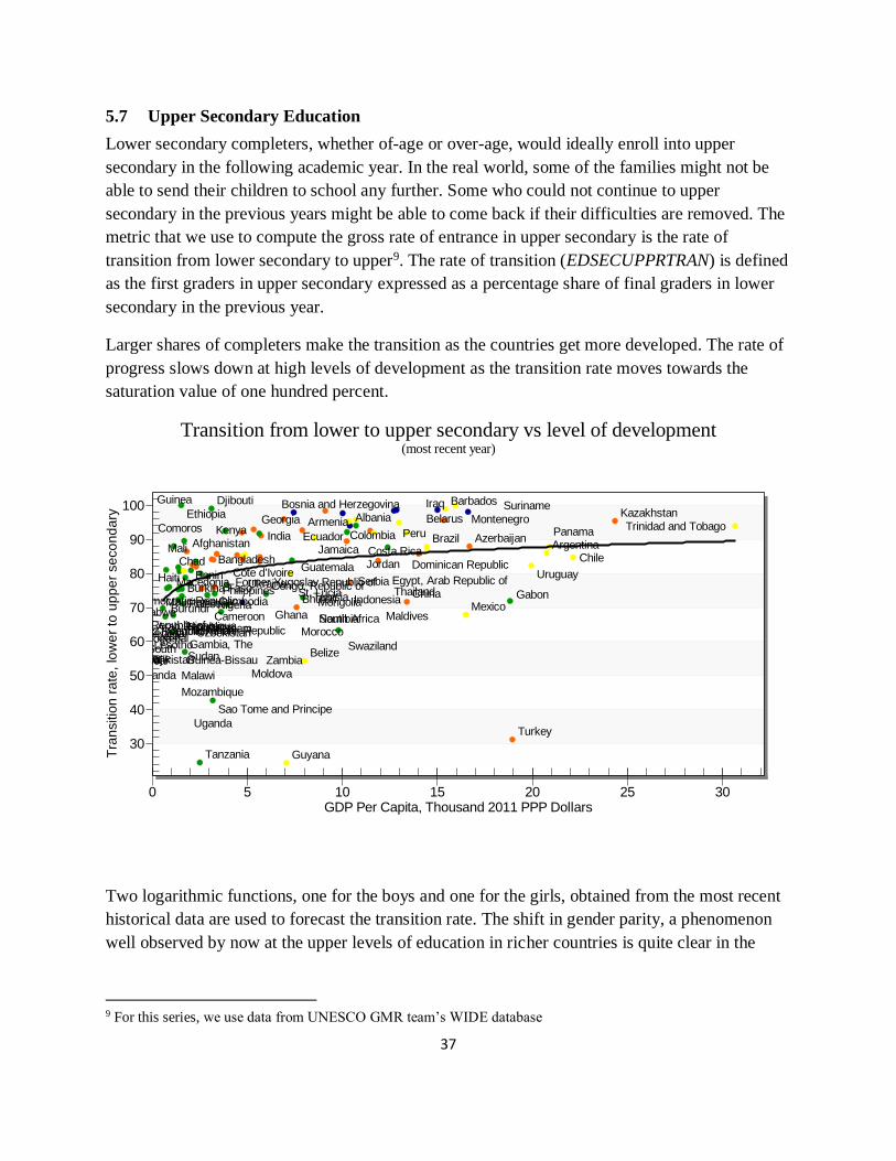
5.7 Upper Secondary Education
Lower secondary completers, whether of-age or over-age, would ideally enroll into upper
secondary in the following academic year. In the real world, some of the families might not be
able to send their children to school any further. Some who could not continue to upper
secondary in the previous years might be able to come back if their difficulties are removed. The
metric that we use to compute the gross rate of entrance in upper secondary is the rate of
transition from lower secondary to upper9. The rate of transition (EDSECUPPRTRAN) is defined
as the first graders in upper secondary expressed as a percentage share of final graders in lower
secondary in the previous year.
Larger shares of completers make the transition as the countries get more developed. The rate of
progress slows down at high levels of development as the transition rate moves towards the
saturation value of one hundred percent.
Two logarithmic functions, one for the boys and one for the girls, obtained from the most recent
historical data are used to forecast the transition rate. The shift in gender parity, a phenomenon
well observed by now at the upper levels of education in richer countries is quite clear in the
9 For this series, we use data from UNESCO GMR team’s WIDE database
Afghanistan
Albania
Argentina
Armenia
Azerbaijan
Bangladesh
Barbados
Belarus
Belize
Benin
Bhutan
Bosnia and Herzegovina
Brazil
Burkina Faso
Burundi Cambodia
Cameroon
Central African Republic
Chad Chile
China
Colombia Comoros
Congo, Democratic Republic of
Congo, Republic of
Costa Rica
Cote d'Ivoire
Djibouti
Dominican Republic
Ecuador
Egypt, Arab Republic of
Ethiopia
Gabon
Gambia, The
Georgia
Ghana
Guatemala
Guinea
Guinea-Bissau
Guyana
Haiti
Honduras
India
Indonesia
Iraq
Jamaica
Jordan
Kazakhstan
Kenya
Kyrgyz Republic
Laos, People's Democratic Republic
Lesotho
Liberia
Macedonia, Former Yugoslav Republic of
Madagascar
Malawi
Maldives
Mali
Mauritania Mexico
Moldova
Mongolia
Montenegro
Morocco
Mozambique
Namibia
Nepal Nicaragua
Niger
Nigeria
Pakistan
Palestine
Panama Peru
Philippines
Rwanda
Sao Tome and Principe
Senegal
Serbia
Sierra Leone
South Africa
St. Lucia
Sudan Sudan South
Suriname
Swaziland
Syrian Arab Republic
Tajikistan
Tanzania
Thailand
Timor-Leste Togo
Trinidad and Tobago
Tunisia
Turkey Uganda
Ukraine Uruguay
Uzbekistan Vietnam Yemen, Republic of
Zambia
Zimbabwe
30
40
50
60
70
80
90
100
0 5 10 15 20 25 30
Transition from lower to upper secondary vs level of development(most recent year)
Tra
nsitio
n r
ate
, lo
we
r to
up
pe
r se
co
nd
ary
GDP Per Capita, Thousand 2011 PPP Dollars
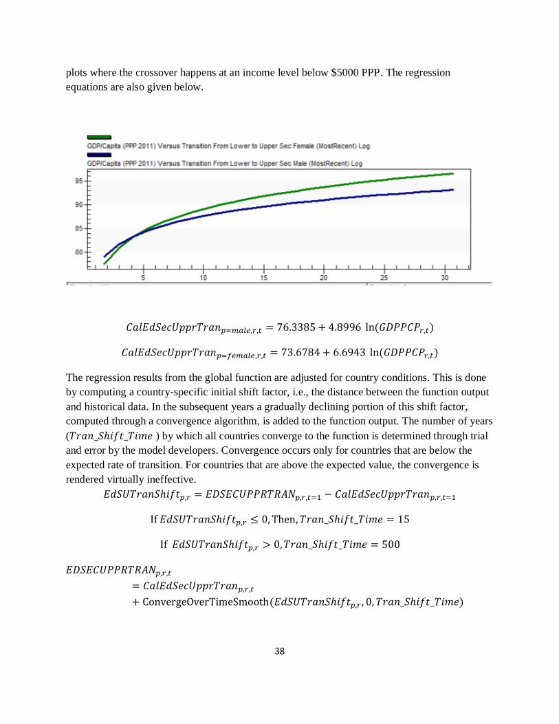
38
plots where the crossover happens at an income level below $5000 PPP. The regression
equations are also given below.
𝐶𝑎𝑙𝐸𝑑𝑆𝑒𝑐𝑈𝑝𝑝𝑟𝑇𝑟𝑎𝑛𝑝=𝑚𝑎𝑙𝑒,𝑟,𝑡 = 76.3385 + 4.8996 ln(𝐺𝐷𝑃𝑃𝐶𝑃𝑟,𝑡)
𝐶𝑎𝑙𝐸𝑑𝑆𝑒𝑐𝑈𝑝𝑝𝑟𝑇𝑟𝑎𝑛𝑝=𝑓𝑒𝑚𝑎𝑙𝑒,𝑟,𝑡 = 73.6784 + 6.6943 ln(𝐺𝐷𝑃𝑃𝐶𝑃𝑟,𝑡)
The regression results from the global function are adjusted for country conditions. This is done
by computing a country-specific initial shift factor, i.e., the distance between the function output
and historical data. In the subsequent years a gradually declining portion of this shift factor,
computed through a convergence algorithm, is added to the function output. The number of years
(𝑇𝑟𝑎𝑛_𝑆ℎ𝑖𝑓𝑡_𝑇𝑖𝑚𝑒 ) by which all countries converge to the function is determined through trial
and error by the model developers. Convergence occurs only for countries that are below the
expected rate of transition. For countries that are above the expected value, the convergence is
rendered virtually ineffective.
𝐸𝑑𝑆𝑈𝑇𝑟𝑎𝑛𝑆ℎ𝑖𝑓𝑡𝑝,𝑟 = 𝐸𝐷𝑆𝐸𝐶𝑈𝑃𝑃𝑅𝑇𝑅𝐴𝑁𝑝,𝑟,𝑡=1 − 𝐶𝑎𝑙𝐸𝑑𝑆𝑒𝑐𝑈𝑝𝑝𝑟𝑇𝑟𝑎𝑛𝑝,𝑟,𝑡=1
If 𝐸𝑑𝑆𝑈𝑇𝑟𝑎𝑛𝑆ℎ𝑖𝑓𝑡𝑝,𝑟 ≤ 0, Then, 𝑇𝑟𝑎𝑛_𝑆ℎ𝑖𝑓𝑡_𝑇𝑖𝑚𝑒 = 15
If 𝐸𝑑𝑆𝑈𝑇𝑟𝑎𝑛𝑆ℎ𝑖𝑓𝑡𝑝,𝑟 > 0, 𝑇𝑟𝑎𝑛_𝑆ℎ𝑖𝑓𝑡_𝑇𝑖𝑚𝑒 = 500
𝐸𝐷𝑆𝐸𝐶𝑈𝑃𝑃𝑅𝑇𝑅𝐴𝑁𝑝,𝑟,𝑡
= 𝐶𝑎𝑙𝐸𝑑𝑆𝑒𝑐𝑈𝑝𝑝𝑟𝑇𝑟𝑎𝑛𝑝,𝑟,𝑡
+ ConvergeOverTimeSmooth(𝐸𝑑𝑆𝑈𝑇𝑟𝑎𝑛𝑆ℎ𝑖𝑓𝑡𝑝,𝑟 , 0, 𝑇𝑟𝑎𝑛_𝑆ℎ𝑖𝑓𝑡_𝑇𝑖𝑚𝑒)
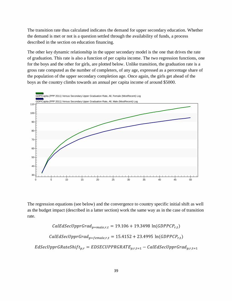
39
The transition rate thus calculated indicates the demand for upper secondary education. Whether
the demand is met or not is a question settled through the availability of funds, a process
described in the section on education financing.
The other key dynamic relationship in the upper secondary model is the one that drives the rate
of graduation. This rate is also a function of per capita income. The two regression functions, one
for the boys and the other for girls, are plotted below. Unlike transition, the graduation rate is a
gross rate computed as the number of completers, of any age, expressed as a percentage share of
the population of the upper secondary completion age. Once again, the girls get ahead of the
boys as the country climbs towards an annual per capita income of around $5000.
The regression equations (see below) and the convergence to country specific initial shift as well
as the budget impact (described in a latter section) work the same way as in the case of transition
rate.
𝐶𝑎𝑙𝐸𝑑𝑆𝑒𝑐𝑈𝑝𝑝𝑟𝐺𝑟𝑎𝑑𝑝=𝑚𝑎𝑙𝑒,𝑟,𝑡 = 19.106 + 19.3498 ln(𝐺𝐷𝑃𝑃𝐶𝑃𝑟,𝑡)
𝐶𝑎𝑙𝐸𝑑𝑆𝑒𝑐𝑈𝑝𝑝𝑟𝐺𝑟𝑎𝑑𝑝=𝑓𝑒𝑚𝑎𝑙𝑒,𝑟,𝑡 = 15.4152 + 23.4995 ln(𝐺𝐷𝑃𝑃𝐶𝑃𝑟,𝑡)
𝐸𝑑𝑆𝑒𝑐𝑈𝑝𝑝𝑟𝐺𝑅𝑎𝑡𝑒𝑆ℎ𝑖𝑓𝑡𝑝,𝑟 = 𝐸𝐷𝑆𝐸𝐶𝑈𝑃𝑃𝑅𝐺𝑅𝐴𝑇𝐸𝑝,𝑟,𝑡=1 − 𝐶𝑎𝑙𝐸𝑑𝑆𝑒𝑐𝑈𝑝𝑝𝑟𝐺𝑟𝑎𝑑𝑝,𝑟,𝑡=1
30
40
50
60
70
80
90
100
110
0 5 10 15 20 25 30 35 40 45 50
GDP/Capita (PPP 2011) Versus Secondary Upper Graduation Rate, All, Female (MostRecent) Log
GDP/Capita (PPP 2011) Versus Secondary Upper Graduation Rate, All, Male (MostRecent) Log
40
If 𝐸𝑑𝑆𝑒𝑐𝑈𝑝𝑝𝑟𝐺𝑅𝑎𝑡𝑒𝑆ℎ𝑖𝑓𝑡𝑝,𝑟 ≤ 0, 𝐺𝑟𝑎𝑑_𝑆ℎ𝑖𝑓𝑡_𝑇𝑖𝑚𝑒 = 15
If 𝐸𝑑𝑆𝑒𝑐𝑈𝑝𝑝𝑟𝐺𝑅𝑎𝑡𝑒𝑆ℎ𝑖𝑓𝑡𝑝,𝑟 > 0, 𝐺𝑟𝑎𝑑_𝑆ℎ𝑖𝑓𝑡_𝑇𝑖𝑚𝑒 = 500
EDSECUPPRGRATE𝑔,𝑟,𝑡
= CalEdSecUpprGrad𝑔,𝑟,𝑡
+ 𝐶𝑜𝑛𝑣𝑒𝑟𝑔𝑒𝑂𝑣𝑒𝑟𝑇𝑖𝑚𝑒𝑆𝑚𝑜𝑜𝑡ℎ(EdSecUpprGRateShift𝑔,𝑟 , 0, Grad_Shift_Time)
Transition rate (EDSECUPPRTRAN) is used to deduce the rate of entrance into upper secondary
(caledsecint) and the gender-specific graduation rate (EDSECUPPRGRATE) helps compute
drop-out rates by gender. The computation steps are shown below. Subscript notation used in
these equations have the same meaning as in the other parts of this document (p is for gender, r
for country or region, t for time and d for grade, c for single-year age cohorts).
𝑐𝑎𝑙𝑒𝑑𝑠𝑒𝑐𝑖𝑛𝑡𝑝,𝑟,𝑡 = 𝑠𝑒𝑐𝑙𝑜𝑤𝑟𝑠𝑡𝑢𝑑𝑒𝑛𝑡𝑠𝑒𝑑𝑠𝑒𝑐𝑙𝑜𝑤𝑟𝑙𝑒𝑛𝑟 ,𝑟,𝑡−1 ∗ 𝐸𝐷𝑆𝐸𝐶𝑈𝑃𝑃𝑅𝑇𝑅𝐴𝑁𝑝,𝑟,𝑡
𝐷𝑟𝑜𝑝𝑜𝑢𝑡𝑅𝑎𝑡𝑒𝑝,𝑟,𝑡 = 1 − (𝐸𝐷𝑆𝐸𝐶𝑈𝑃𝑃𝑅𝐺𝑅𝐴𝑇𝐸𝑝,𝑟,𝑡
𝑐𝑎𝑙𝑒𝑑𝑠𝑒𝑐𝑖𝑛𝑡𝑝,𝑟,𝑡)
1𝒆𝒅𝒔𝒆𝒄𝒖𝒑𝒑𝒓𝒍𝒆𝒏𝑟−1
𝑠𝑒𝑐𝑢𝑝𝑝𝑟𝑠𝑡𝑢𝑑𝑒𝑛𝑡𝑠𝑑=1,𝑝,𝑟,𝑡 = 𝑐𝑎𝑙𝑒𝑑𝑠𝑒𝑐𝑖𝑛𝑡𝑝,𝑟,𝑡
𝑠𝑒𝑐𝑢𝑝𝑝𝑟𝑠𝑡𝑢𝑑𝑒𝑛𝑡𝑠𝑑,𝑝,𝑟,𝑡 = 𝑠𝑒𝑐𝑢𝑝𝑝𝑟𝑠𝑡𝑢𝑑𝑒𝑛𝑡𝑠𝑑−1,𝑝,𝑟,𝑡−1 ∗ (1 − 𝐷𝑟𝑜𝑝𝑜𝑢𝑡𝑅𝑎𝑡𝑒𝑝,𝑟,𝑡)
𝑒𝑑𝑠𝑒𝑐𝑢𝑝𝑝𝑟𝑝𝑜𝑝𝑝,𝑟,𝑡 = ∑ 𝑓𝑎𝑔𝑒𝑑𝑠𝑡𝑐,𝑝,𝑟,𝑡
𝒆𝒅𝒑𝒓𝒊𝒔𝒕𝒂𝒓𝒕𝑟+ 𝒆𝒅𝒑𝒓𝒊𝒍𝒆𝒏𝑟+𝒆𝒅𝒔𝒆𝒄𝒍𝒐𝒘𝒓𝒍𝒆𝒏𝑟+𝒆𝒅𝒔𝒆𝒄𝒖𝒑𝒑𝒓𝒍𝒆𝒏𝑟
𝑐 = 𝒆𝒅𝒑𝒓𝒊𝒔𝒕𝒂𝒓𝒕𝑟+ 𝒆𝒅𝒑𝒓𝒊𝒍𝒆𝒏𝑟+𝒆𝒅𝒔𝒆𝒄𝒍𝒐𝒘𝒓𝒍𝒆𝒏𝑟
𝐸𝐷𝑆𝐸𝐶𝑈𝑃𝑃𝑅𝑇𝑂𝑇𝑝,𝑟,𝑡
= ∑ ( 𝑠𝑒𝑐𝑢𝑝𝑝𝑟𝑠𝑡𝑢𝑑𝑒𝑛𝑡𝑠𝑑,𝑝,𝑟,𝑡
𝒆𝒅𝒔𝒆𝒄𝒖𝒑𝒑𝒓𝒍𝒆𝒏𝑟
𝑑=1
∗ 𝑓𝑎𝑔𝑒𝑑𝑠𝑡 𝑑+ 𝑒𝑑𝑝𝑟𝑖𝑠𝑡𝑎𝑟𝑡𝑟+ 𝑒𝑑𝑝𝑟𝑖𝑙𝑒𝑛𝑟+ 𝑒𝑑𝑠𝑒𝑐𝑙𝑜𝑤𝑟𝑙𝑒𝑛𝑟 ,𝑝,𝑟,𝑡)
𝐸𝐷𝑆𝐸𝐶𝑈𝑃𝑃𝑅𝐸𝑁𝑅𝐺𝑝,𝑟,𝑡 = 100 ∗ 𝐸𝐷𝑆𝐸𝐶𝑈𝑃𝑃𝑅𝑇𝑂𝑇𝑝,𝑟,𝑡 / 𝑒𝑑𝑠𝑒𝑐𝑢𝑝𝑝𝑟𝑝𝑜𝑝𝑝,𝑟,𝑡
41
5.8 Secondary Education: Vocational Education
Lower and upper secondary education are further divided into a general and a vocational
curriculum. Country specific vocational participation data collected from UNESCO Institute for
Statistics do not show any common trend in provision or attainment of vocational education
across the world. The existence, expansion or phase-out of vocational education in a country
results from policy decisions that cannot be modeled analytically. We implement a simple
representation of vocational education in the model through a vocational share of total
enrollment for lower secondary (EDSECLOWRVOC) and upper secondary (EDSECUPPRVOC).
These vocational shares are initialized with UNESCO data. We assume the vocational shares to
be zero when no data is available. The model projects the shares to be constant over time across
the entire forecasting horizon.
The vocational shares can be changed through exogenous country-specific parameters, one for
lower secondary (edseclowrvocadd) and one for upper secondary (edsecupprvocadd). These
additive parameters can be set to negative or positive values to raise or lower the percentage
share of vocational in total enrollment. Changed vocational shares are bound to an upper limit of
seventy percent. This upper bound reflects the maximum value of vocational share in the
historical data. The upper secondary vocational share in Germany, which at about 67% is the
largest among all vocational shares for which we have data.
𝐸𝐷𝑆𝐸𝐶𝐿𝑂𝑊𝑅𝑉𝑂𝐶𝐼𝑝,𝑟 = 𝐸𝐷𝑆𝐸𝐶𝐿𝑂𝑊𝑅𝑉𝑂𝐶𝑝,𝑟,𝑡=1
𝐸𝐷𝑆𝐸𝐶𝐿𝑂𝑊𝑅𝑉𝑂𝐶𝑝,𝑟,𝑡 = Amax ( 70, 𝐸𝐷𝑆𝐸𝐶𝐿𝑂𝑊𝑅𝑉𝑂𝐶𝐼𝑝,𝑟 + 𝑒𝑑𝑠𝑒𝑐𝑙𝑜𝑤𝑟𝑣𝑜𝑐𝑎𝑑𝑑𝑝,𝑟,𝑡)
5.9 Secondary Education: Total Secondary
The gross enrollment rate in the entire secondary (EDSECENRG) is computed by summing up
the total enrollment in lower and upper secondary and then dividing that sum by the total
secondary-age population (secpop).
𝐸𝐷𝑆𝐸𝐶𝑇𝑂𝑇𝑝,𝑟,𝑡 = 𝐸𝐷𝑆𝐸𝐶𝐿𝑂𝑊𝑅𝑇𝑂𝑇𝑝,𝑟,𝑡 + 𝐸𝐷𝑆𝐸𝐶𝑈𝑃𝑃𝑅𝑇𝑂𝑇𝑝,𝑟,𝑡
𝑠𝑒𝑐𝑝𝑜𝑝 = 𝑠𝑒𝑐𝑙𝑜𝑤𝑟𝑝𝑜𝑝𝑝,𝑟,𝑡 + 𝑠𝑒𝑐𝑢𝑝𝑝𝑟𝑝𝑜𝑝𝑝,𝑟,𝑡
𝐸𝐷𝑆𝐸𝐶𝐸𝑁𝑅𝐺𝑝,𝑟,𝑡 = (𝐸𝐷𝑆𝐸𝐶𝐿𝑂𝑊𝑅𝑇𝑂𝑇𝑝,𝑟,𝑡 + 𝐸𝐷𝑆𝐸𝐶𝑈𝑃𝑃𝑅𝑇𝑂𝑇𝑝,𝑟,𝑡)/secpop
Net enrollment rate in secondary is then computed through an analytic function driven by gross
enrollment rate.
𝐸𝐷𝑆𝐸𝐶𝐸𝑁𝑅𝑁𝑝,𝑟,𝑡 = f(𝐸𝐷𝑆𝐸𝐶𝐸𝑁𝑅𝐺𝑝,𝑟,𝑡)
42
5.10 Education Equations: Tertiary
The model for tertiary education is slightly different from the grade-flow model used for the
elementary and the two secondary levels of education. We could not find any global country-
year data series that can help compute the rate of entrance into tertiary. The high tuition and
opportunity cost prevent substantial number of low income students from enrolling into college
right after high school. Some of those who miss come back for higher education later in life.
Moreover, tertiary education has quite some variation across levels and curricula (ISCED has
three different levels for tertiary education). All of these phenomena might have made the
calculation of an entrance rate difficult for this level. There is, however, good data on
participation and graduation. We forecast a gross enrollment rate and a graduation rate
(EDTERGRATE) for tertiary. A grade-flow distribution is constructed using these two
variables10.
Tertiary enrollment rate (EDTERENRATEG) is driven by the level of development and the upper
secondary completion rate of those who are twenty to twenty-four years old.
𝐶𝑎𝑙𝐸𝑑𝑇𝑒𝑟𝐸𝑛𝑟𝐺1𝑝,𝑟,𝑡 = f(𝐺𝐷𝑃𝑃𝐶𝑃𝑟,𝑡 , 𝐸𝐷𝑆𝐸𝐶𝑃𝐸𝑅20𝑡𝑜24𝑝,𝑟,𝑡−1)
Output from the analytical function is adjusted for country conditions using the same type of
shift convergence algorithm that we use for other student flow rates (see, for example, the
section on the transition rate from lower to upper secondary).
𝐸𝑑𝑇𝑒𝑟𝐸𝑛𝑟𝑔𝑆ℎ𝑖𝑓𝑡𝑝,𝑟 = 𝐸𝐷𝑇𝐸𝑅𝐸𝑁𝑅𝐺𝑝,𝑟,𝑡=1 − 𝐶𝑎𝑙𝐸𝑑𝑇𝑒𝑟𝐸𝑛𝑟𝑔1𝑝,𝑟,𝑡=1
If 𝐸𝑑𝑇𝑒𝑟𝐸𝑛𝑟𝑔𝑆ℎ𝑖𝑓𝑡𝑝,𝑟 ≤ 0, 𝑒𝑑𝑡𝑒𝑟𝑒𝑛𝑟𝑔𝑠ℎ𝑖𝑓𝑡𝐶𝑇𝑖𝑚𝑒𝑝,𝑟 = 25
If 𝐸𝑑𝑇𝑒𝑟𝐸𝑛𝑟𝑔𝑆ℎ𝑖𝑓𝑡𝑝,𝑟 > 0, 𝑒𝑑𝑡𝑒𝑟𝑒𝑛𝑟𝑔𝑠ℎ𝑖𝑓𝑡𝐶𝑇𝑖𝑚𝑒𝑝,𝑟 = 100
𝐸𝐷𝑇𝐸𝑅𝐸𝑁𝑅𝐴𝑇𝐸𝐺𝑝,𝑟,𝑡
= 𝐶𝑎𝑙𝐸𝑑𝑇𝑒𝑟𝐸𝑛𝑟𝑔1𝑝,𝑟,𝑡
+ ConvergeOverTime1(𝐸𝑑𝑇𝑒𝑟𝐸𝑛𝑟𝑔𝑆ℎ𝑖𝑓𝑡𝑝,𝑟 , 0, 𝑒𝑑𝑡𝑒𝑟𝑒𝑛𝑟𝑔𝑠ℎ𝑖𝑓𝑡𝐶𝑇𝑖𝑚𝑒𝑝,𝑟)
Graduation rate for tertiary is determined by the current rate of enrollment at this level
(EDTERENRATEG) and the level of tertiary education (EDTERPER) of the overall population.
10 Grade-flow and drop-outs by grade are used in computing education years.
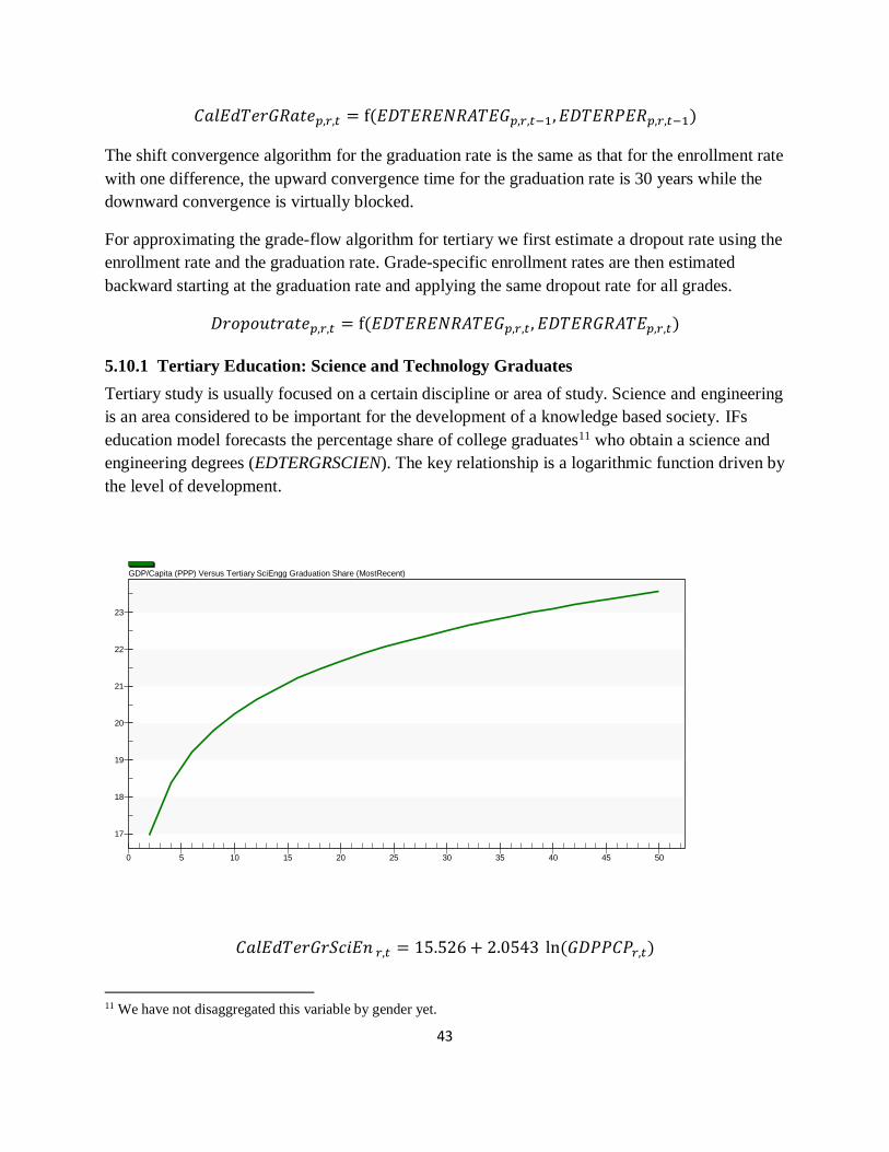
43
𝐶𝑎𝑙𝐸𝑑𝑇𝑒𝑟𝐺𝑅𝑎𝑡𝑒𝑝,𝑟,𝑡 = f(𝐸𝐷𝑇𝐸𝑅𝐸𝑁𝑅𝐴𝑇𝐸𝐺𝑝,𝑟,𝑡−1, 𝐸𝐷𝑇𝐸𝑅𝑃𝐸𝑅𝑝,𝑟,𝑡−1)
The shift convergence algorithm for the graduation rate is the same as that for the enrollment rate
with one difference, the upward convergence time for the graduation rate is 30 years while the
downward convergence is virtually blocked.
For approximating the grade-flow algorithm for tertiary we first estimate a dropout rate using the
enrollment rate and the graduation rate. Grade-specific enrollment rates are then estimated
backward starting at the graduation rate and applying the same dropout rate for all grades.
𝐷𝑟𝑜𝑝𝑜𝑢𝑡𝑟𝑎𝑡𝑒𝑝,𝑟,𝑡 = f(𝐸𝐷𝑇𝐸𝑅𝐸𝑁𝑅𝐴𝑇𝐸𝐺𝑝,𝑟,𝑡 , 𝐸𝐷𝑇𝐸𝑅𝐺𝑅𝐴𝑇𝐸𝑝,𝑟,𝑡)
5.10.1 Tertiary Education: Science and Technology Graduates
Tertiary study is usually focused on a certain discipline or area of study. Science and engineering
is an area considered to be important for the development of a knowledge based society. IFs
education model forecasts the percentage share of college graduates11 who obtain a science and
engineering degrees (EDTERGRSCIEN). The key relationship is a logarithmic function driven by
the level of development.
𝐶𝑎𝑙𝐸𝑑𝑇𝑒𝑟𝐺𝑟𝑆𝑐𝑖𝐸𝑛 𝑟,𝑡 = 15.526 + 2.0543 ln(𝐺𝐷𝑃𝑃𝐶𝑃𝑟,𝑡)
11 We have not disaggregated this variable by gender yet.
17
18
19
20
21
22
23
0 5 10 15 20 25 30 35 40 45 50
GDP/Capita (PPP) Versus Tertiary SciEngg Graduation Share (MostRecent)

44
This forecast is also adjusted for country conditions with the initial shift factor and a
convergence algorithm like we do with other flow rates.
There is an additive parameter12 (edterscienshradd), with a base case value of zero, that can be
used tochange the percentage share of science and engineering among tertiary graduates. This
parameter does not have any effect on the total number of tertiary graduates (EDTERGRADS).
5.11 Education Equations: Budget Flow
Education model computes the demand for funds, using student headcounts and per student
costs, and send the demand (EDBUDDEM) to the government finance model. Government
finance model handles the distribution of government consumption spending across different
public sectors like defense, health, education, R&D and infrastructure. Back in the education
model, total educational allocation is distributed among the four different levels of education
using a normalization algorithm. Deficit or surplus, if there is any, first impacts student flow
rates; the grade-flows are adjusted accordingly. Any residual of the budget impact goes to per
student costs. Total spending in education (EDTOTCOST) is recomputed at the end of this
process.
5.11.1 Per Student Cost
The major portion of public spending in education goes towards teacher salary. Salaries move
with the average income in a country. Per student public costs for the four different levels of
education, expressed as percentages of per capita income, change in our model through four
regression functions drawn with most recent historical data. The independent variable for all of
these bi-variate regressions is per capita income expressed in thousand PPP dollars. The figure
below plots all these functions.
12 The parameter seems to be inactive (version 7.30)
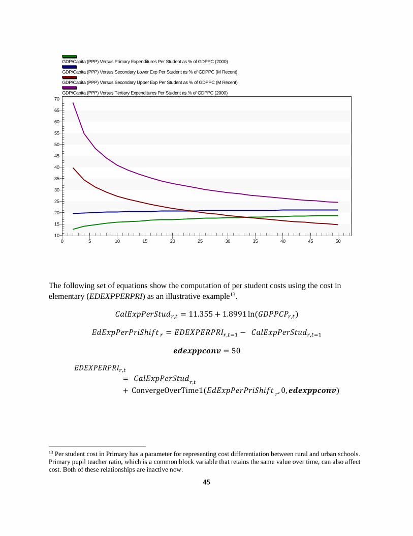
45
The following set of equations show the computation of per student costs using the cost in
elementary (EDEXPPERPRI) as an illustrative example13.
𝐶𝑎𝑙𝐸𝑥𝑝𝑃𝑒𝑟𝑆𝑡𝑢𝑑𝑟,𝑡 = 11.355 + 1.8991 ln(𝐺𝐷𝑃𝑃𝐶𝑃𝑟,𝑡)
𝐸𝑑𝐸𝑥𝑝𝑃𝑒𝑟𝑃𝑟𝑖𝑆ℎ𝑖𝑓𝑡 𝑟 = 𝐸𝐷𝐸𝑋𝑃𝐸𝑅𝑃𝑅𝐼𝑟,𝑡=1 − 𝐶𝑎𝑙𝐸𝑥𝑝𝑃𝑒𝑟𝑆𝑡𝑢𝑑𝑟,𝑡=1
𝒆𝒅𝒆𝒙𝒑𝒑𝒄𝒐𝒏𝒗 = 50
𝐸𝐷𝐸𝑋𝑃𝐸𝑅𝑃𝑅𝐼𝑟,𝑡
= 𝐶𝑎𝑙𝐸𝑥𝑝𝑃𝑒𝑟𝑆𝑡𝑢𝑑𝑟,𝑡
+ ConvergeOverTime1(𝐸𝑑𝐸𝑥𝑝𝑃𝑒𝑟𝑃𝑟𝑖𝑆ℎ𝑖𝑓𝑡 𝑟, 0, 𝒆𝒅𝒆𝒙𝒑𝒑𝒄𝒐𝒏𝒗)
13 Per student cost in Primary has a parameter for representing cost differentiation between rural and urban schools.
Primary pupil teacher ratio, which is a common block variable that retains the same value over time, can also affect
cost. Both of these relationships are inactive now.
10
15
20
25
30
35
40
45
50
55
60
65
70
0 5 10 15 20 25 30 35 40 45 50
GDP/Capita (PPP) Versus Primary Expenditures Per Student as % of GDPPC (2000)
GDP/Capita (PPP) Versus Secondary Lower Exp Per Student as % of GDPPC (M Recent)
GDP/Capita (PPP) Versus Secondary Upper Exp Per Student as % of GDPPC (M Recent)
GDP/Capita (PPP) Versus Tertiary Expenditures Per Student as % of GDPPC (2000)
46
5.11.2 Budget Demand
Demand for educational spending is computed from the projections of enrollment and per
student cost for the four levels of education.
𝑢𝑑_𝐷𝑒𝑚𝑎𝑛𝑑𝑃𝑟𝑖𝑟,𝑡 = 𝑈𝐷_𝐸𝐷𝐸𝑥𝑝𝑃𝑒𝑟𝑃𝑟𝑖𝑟,𝑡 ∗ 𝐺𝐷𝑃𝑃𝐶𝑃𝑟,𝑡 ∗ ∑ 𝑈𝐷_𝐸𝑛𝑟𝑜𝑙𝑙𝐶𝑇𝑝𝑟𝑖𝑚𝑎𝑟𝑦,𝑝,𝑟,𝑡 100⁄
2
𝑝=1
𝑢𝑑_𝐷𝑒𝑚𝑎𝑛𝑑𝑆𝑒𝑐𝐿𝑜𝑤𝑟𝑟,𝑡
= 𝑈𝐷_𝐸𝐷𝐸𝑥𝑝𝑃𝑒𝑟𝑆𝑒𝑐𝐿𝑜𝑤𝑟𝑟,𝑡 ∗ 𝐺𝐷𝑃𝑃𝐶𝑃𝑟,𝑡 ∗ ∑ 𝑈𝐷_𝐸𝑛𝑟𝑜𝑙𝑙𝐶𝑇𝑠𝑒𝑐𝑙𝑜𝑤𝑟,𝑝,𝑟,𝑡 100⁄
2
𝑝=1
𝑢𝑑_𝐷𝑒𝑚𝑎𝑛𝑑𝑆𝑒𝑐𝑈𝑝𝑝𝑟𝑟,𝑡
= 𝑈𝐷_𝐸𝐷𝐸𝑥𝑝𝑃𝑒𝑟𝑆𝑒𝑐𝑈𝑝𝑝𝑟𝑟,𝑡 ∗ 𝐺𝐷𝑃𝑃𝐶𝑃𝑟,𝑡 ∗ ∑ 𝑈𝐷_𝐸𝑛𝑟𝑜𝑙𝑙𝐶𝑇𝑠𝑒𝑐𝑢𝑝𝑝𝑟,𝑝,𝑟,𝑡 100⁄
2
𝑝=1
𝑢𝑑_𝐷𝑒𝑚𝑎𝑛𝑑𝑆𝑒𝑐𝑟,𝑡 = 𝑢𝑑_𝐷𝑒𝑚𝑎𝑛𝑑𝑆𝑒𝑐𝐿𝑜𝑤𝑟𝑟,𝑡 + 𝑢𝑑_𝐷𝑒𝑚𝑎𝑛𝑑𝑆𝑒𝑐𝑈𝑝𝑝𝑟𝑟,𝑡
𝑢𝑑_𝐷𝑒𝑚𝑎𝑛𝑑𝑇𝑒𝑟𝑟,𝑡 = 𝑈𝐷_𝐸𝐷𝐸𝑥𝑝𝑃𝑒𝑟𝑇𝑒𝑟𝑟,𝑡 ∗ 𝐺𝐷𝑃𝑃𝐶𝑃𝑟,𝑡 ∗ ∑ 𝑈𝐷_𝐸𝑛𝑟𝑜𝑙𝑙𝐶𝑇𝑡𝑒𝑟𝑡𝑖𝑎𝑟𝑦,𝑝,𝑟,𝑡 100⁄
2
𝑝=1
𝐸𝐷𝐵𝑈𝐷𝐷𝐸𝑀𝑟,𝑡 = 𝑢𝑑_𝐷𝑒𝑚𝑎𝑛𝑑𝑃𝑟𝑖𝑟,𝑡 + 𝑢𝑑_𝐷𝑒𝑚𝑎𝑛𝑑𝑆𝑒𝑐𝑟,𝑡 + 𝑢𝑑_𝐷𝑒𝑚𝑎𝑛𝑑𝑇𝑒𝑟𝑟,𝑡
5.11.3 Budget Allocation Across Sectors of Spending
Total fund demand (EDBUDDEM) is passed to the IFs socio-political model where a detail
government budget model distributes total government consumption among various public
expenditure sectors using a normalization algorithm described in the government finance model
documentation. Distribution to education is prioritized in the base case of the model with a
protection of at least 40% of the budget demanded through a model parameter (gdsbudgetprotec)
that can be changed by model user between 0 to 100%.
5.11.3.1 Educational Budget Allocation: Top-Down versus Bottom-up
Another feature of budget distribution is the reconciliation between allocation on education given
the level of development of the country, we call it top-down, and the budget demand projected in
the education model, we call it bottom-up. The top-down number is obtained from a regression
of educational spending (as a percentage share of total GDP) driven by per capita income
(GDPPCP). This is adjusted for country condition using a multiplicative shift factor computed in
47
the first year from the ratios of historical data on spending in education (GDS) and function
output (gkcomp).
𝑔𝑘𝑐𝑜𝑚𝑝𝑟,𝑔=𝐸𝑑𝑢𝑐,𝑡 = f(𝐺𝐷𝑃𝑃𝐶𝑃𝑟,𝑡)
𝑔𝑘𝑟𝑖𝑟,𝑔=𝐸𝑑𝑢𝑐 = 𝐺𝐷𝑆𝑟,𝑔=𝐸𝑑𝑢𝑐,𝑡=1 𝐺𝐷𝑃𝑟,𝑡=1 𝑔𝑘𝑐𝑜𝑚𝑝𝑟,𝑔=𝐸𝑑𝑢𝑐,𝑡=1⁄⁄
𝑔𝑘𝑠ℎ𝑖𝑓𝑡𝑟,𝑡,𝑔=𝐸𝑑𝑢𝑐 = 𝐶𝑜𝑛𝑣𝑒𝑟𝑔𝑒𝑂𝑣𝑒𝑟𝑇𝑖𝑚𝑒(𝑔𝑘𝑟𝑖𝑟,𝑔=𝐸𝑑𝑢𝑐, 75,1)
𝐺𝐷𝑆𝑟,𝑔=𝐸𝑑𝑢𝑐,𝑡 = 𝑔𝑘𝑐𝑜𝑚𝑝𝑟,𝑔=𝐸𝑑𝑢𝑐,𝑡 ∗ 𝑔𝑘𝑠ℎ𝑖𝑓𝑡𝑟,𝑡,𝑔=𝐸𝑑𝑢𝑐 ∗ 𝐺𝐷𝑃𝑟,𝑡 100⁄
There is a lag of one year between the budget demand calculated in the education model and the
use of the demand in the government finance model. This lag is a code-sequence issue and
compensated through a growth rate term (EcGrTerm).
𝑠𝐸𝑑𝑇𝑜𝑡𝐶𝑜𝑠𝑡𝑟,𝑡 = 𝐸𝐷𝐵𝑈𝐷𝐷𝐸𝑀𝑟,𝑡−1
𝐷𝑒𝑚𝑎𝑛𝑑𝐶𝑎𝑙𝑐 = 𝑠𝐸𝑑𝑇𝑜𝑡𝐶𝑜𝑠𝑡𝑟,𝑡 ∗ (1 + 𝐸𝑐𝐺𝑟𝑇𝑒𝑟𝑚𝑟,𝑡) ∗ 𝐸𝑑𝐶𝑜𝑠𝑡𝐺𝐷𝑆𝐸𝑑𝑅𝐼𝑟,𝑡
where,
𝐸𝑐𝐺𝑟𝑇𝑒𝑟𝑚𝑟,𝑡 = ConvergeoverTime(𝑖𝑔𝑑𝑝𝑟𝑟 , 0 , 50)
And EdCostGDSEdRI is a term representing the initial ratio of the bottom-up and the top-down
calculation.
5.11.3.2 Educational Budget Prioritization
A normalization algorithm is used to distribute the total available government consumption
budget (GOVCON) among all sector spending (GDS, g is the subscript for spending sectors).
Prior to the normalization, a priority parameter (gdsbudgetprotec) allows setting aside all or part
of demanded funds for the spending sectors. Forty percent of educational demands are set aside
in the model base case.
𝐺𝑇𝑂𝑇 = ∑ 𝐺𝐷𝑆𝑟,𝑔,𝑡
𝑁𝐺𝑜𝑣𝐸𝑥𝑝
𝑔=1
𝐺𝐷𝑆𝑆𝑒𝑡𝐴𝑠𝑖𝑑𝑒𝑟,𝑔,𝑡 = 𝐺𝐷𝑆𝑟,𝑔,𝑡 ∗ (1 − 𝑔𝑑𝑠𝑏𝑢𝑑𝑔𝑒𝑡𝑝𝑟𝑜𝑡𝑒𝑐𝑟,𝑔,𝑡)
𝑇𝑜𝑡𝑆𝑒𝑡𝐴𝑠𝑖𝑑𝑒 = ∑ 𝐺𝐷𝑆𝑆𝑒𝑡𝐴𝑠𝑖𝑑𝑒𝑟,𝑔,𝑡
𝑁𝐺𝑜𝑣𝐸𝑥𝑝
𝑔=1
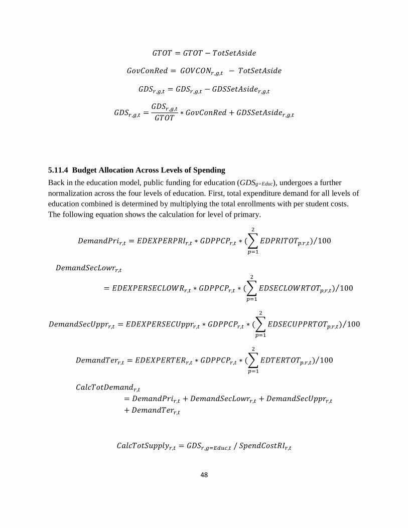
48
𝐺𝑇𝑂𝑇 = 𝐺𝑇𝑂𝑇 − 𝑇𝑜𝑡𝑆𝑒𝑡𝐴𝑠𝑖𝑑𝑒
𝐺𝑜𝑣𝐶𝑜𝑛𝑅𝑒𝑑 = 𝐺𝑂𝑉𝐶𝑂𝑁𝑟,𝑔,𝑡 − 𝑇𝑜𝑡𝑆𝑒𝑡𝐴𝑠𝑖𝑑𝑒
𝐺𝐷𝑆𝑟,𝑔,𝑡 = 𝐺𝐷𝑆𝑟,𝑔,𝑡 − 𝐺𝐷𝑆𝑆𝑒𝑡𝐴𝑠𝑖𝑑𝑒𝑟,𝑔,𝑡
𝐺𝐷𝑆𝑟,𝑔,𝑡 =𝐺𝐷𝑆𝑟,𝑔,𝑡
𝐺𝑇𝑂𝑇∗ 𝐺𝑜𝑣𝐶𝑜𝑛𝑅𝑒𝑑 + 𝐺𝐷𝑆𝑆𝑒𝑡𝐴𝑠𝑖𝑑𝑒𝑟,𝑔,𝑡
5.11.4 Budget Allocation Across Levels of Spending
Back in the education model, public funding for education (GDSg=Educ), undergoes a further
normalization across the four levels of education. First, total expenditure demand for all levels of
education combined is determined by multiplying the total enrollments with per student costs.
The following equation shows the calculation for level of primary.
𝐷𝑒𝑚𝑎𝑛𝑑𝑃𝑟𝑖𝑟,𝑡 = 𝐸𝐷𝐸𝑋𝑃𝐸𝑅𝑃𝑅𝐼𝑟,𝑡 ∗ 𝐺𝐷𝑃𝑃𝐶𝑃𝑟,𝑡 ∗ (∑ 𝐸𝐷𝑃𝑅𝐼𝑇𝑂𝑇𝑝.𝑟,𝑡) 100⁄
2
𝑝=1
𝐷𝑒𝑚𝑎𝑛𝑑𝑆𝑒𝑐𝐿𝑜𝑤𝑟𝑟,𝑡
= 𝐸𝐷𝐸𝑋𝑃𝐸𝑅𝑆𝐸𝐶𝐿𝑂𝑊𝑅𝑟,𝑡 ∗ 𝐺𝐷𝑃𝑃𝐶𝑃𝑟,𝑡 ∗ (∑ 𝐸𝐷𝑆𝐸𝐶𝐿𝑂𝑊𝑅𝑇𝑂𝑇𝑝,𝑟,𝑡) 100⁄
2
𝑝=1
𝐷𝑒𝑚𝑎𝑛𝑑𝑆𝑒𝑐𝑈𝑝𝑝𝑟𝑟,𝑡 = 𝐸𝐷𝐸𝑋𝑃𝐸𝑅𝑆𝐸𝐶𝑈𝑝𝑝𝑟𝑟,𝑡 ∗ 𝐺𝐷𝑃𝑃𝐶𝑃𝑟,𝑡 ∗ (∑ 𝐸𝐷𝑆𝐸𝐶𝑈𝑃𝑃𝑅𝑇𝑂𝑇𝑝,𝑟,𝑡) 100⁄
2
𝑝=1
𝐷𝑒𝑚𝑎𝑛𝑑𝑇𝑒𝑟𝑟,𝑡 = 𝐸𝐷𝐸𝑋𝑃𝐸𝑅𝑇𝐸𝑅𝑟,𝑡 ∗ 𝐺𝐷𝑃𝑃𝐶𝑃𝑟,𝑡 ∗ (∑ 𝐸𝐷𝑇𝐸𝑅𝑇𝑂𝑇𝑝.𝑟,𝑡) 100⁄
2
𝑝=1
𝐶𝑎𝑙𝑐𝑇𝑜𝑡𝐷𝑒𝑚𝑎𝑛𝑑𝑟,𝑡
= 𝐷𝑒𝑚𝑎𝑛𝑑𝑃𝑟𝑖𝑟,𝑡 + 𝐷𝑒𝑚𝑎𝑛𝑑𝑆𝑒𝑐𝐿𝑜𝑤𝑟𝑟,𝑡 + 𝐷𝑒𝑚𝑎𝑛𝑑𝑆𝑒𝑐𝑈𝑝𝑝𝑟𝑟,𝑡
+ 𝐷𝑒𝑚𝑎𝑛𝑑𝑇𝑒𝑟𝑟,𝑡
𝐶𝑎𝑙𝑐𝑇𝑜𝑡𝑆𝑢𝑝𝑝𝑙𝑦𝑟,𝑡 = 𝐺𝐷𝑆𝑟,𝑔=𝐸𝑑𝑢𝑐,𝑡 / 𝑆𝑝𝑒𝑛𝑑𝐶𝑜𝑠𝑡𝑅𝐼𝑟,𝑡
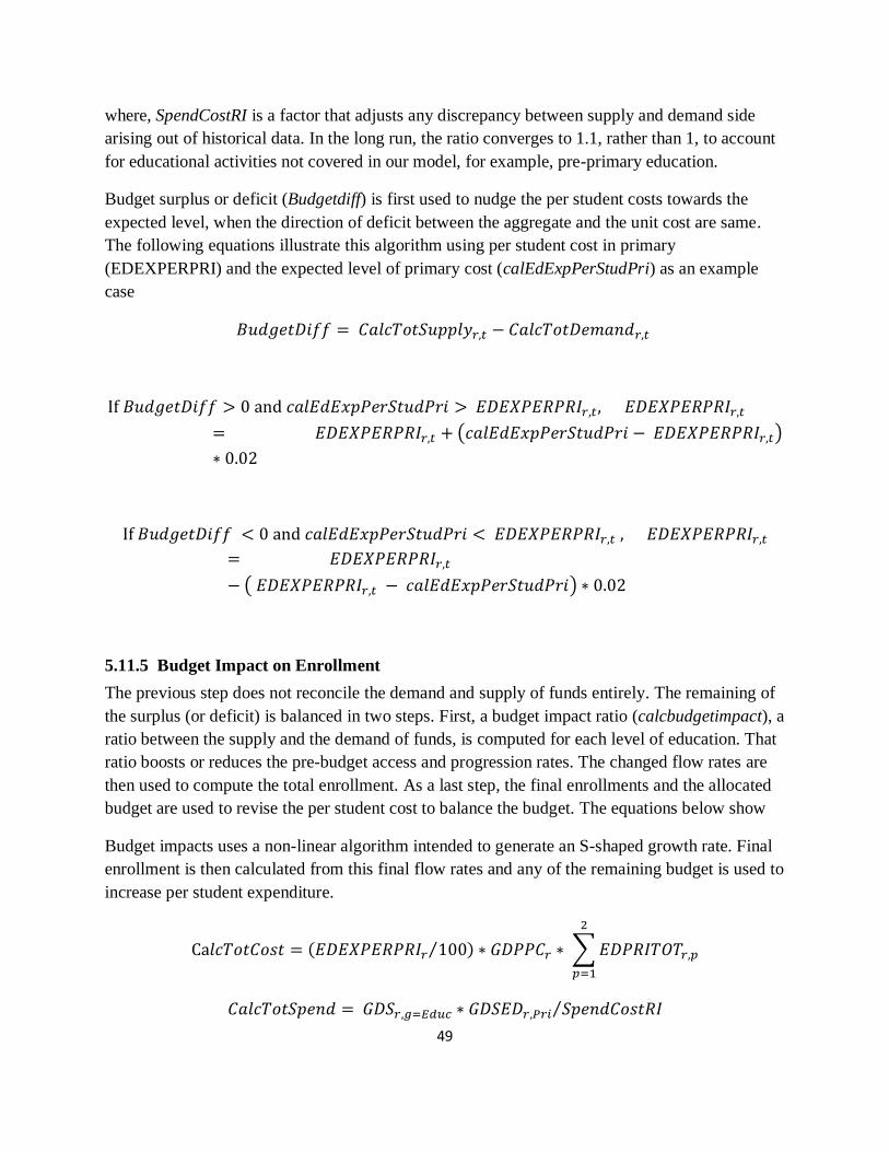
49
where, SpendCostRI is a factor that adjusts any discrepancy between supply and demand side
arising out of historical data. In the long run, the ratio converges to 1.1, rather than 1, to account
for educational activities not covered in our model, for example, pre-primary education.
Budget surplus or deficit (Budgetdiff) is first used to nudge the per student costs towards the
expected level, when the direction of deficit between the aggregate and the unit cost are same.
The following equations illustrate this algorithm using per student cost in primary
(EDEXPERPRI) and the expected level of primary cost (calEdExpPerStudPri) as an example
case
𝐵𝑢𝑑𝑔𝑒𝑡𝐷𝑖𝑓𝑓 = 𝐶𝑎𝑙𝑐𝑇𝑜𝑡𝑆𝑢𝑝𝑝𝑙𝑦𝑟,𝑡 − 𝐶𝑎𝑙𝑐𝑇𝑜𝑡𝐷𝑒𝑚𝑎𝑛𝑑𝑟,𝑡
If 𝐵𝑢𝑑𝑔𝑒𝑡𝐷𝑖𝑓𝑓 > 0 and 𝑐𝑎𝑙𝐸𝑑𝐸𝑥𝑝𝑃𝑒𝑟𝑆𝑡𝑢𝑑𝑃𝑟𝑖 > 𝐸𝐷𝐸𝑋𝑃𝐸𝑅𝑃𝑅𝐼𝑟,𝑡 , 𝐸𝐷𝐸𝑋𝑃𝐸𝑅𝑃𝑅𝐼𝑟,𝑡
= 𝐸𝐷𝐸𝑋𝑃𝐸𝑅𝑃𝑅𝐼𝑟,𝑡 + (𝑐𝑎𝑙𝐸𝑑𝐸𝑥𝑝𝑃𝑒𝑟𝑆𝑡𝑢𝑑𝑃𝑟𝑖 − 𝐸𝐷𝐸𝑋𝑃𝐸𝑅𝑃𝑅𝐼𝑟,𝑡)
∗ 0.02
If 𝐵𝑢𝑑𝑔𝑒𝑡𝐷𝑖𝑓𝑓 < 0 and 𝑐𝑎𝑙𝐸𝑑𝐸𝑥𝑝𝑃𝑒𝑟𝑆𝑡𝑢𝑑𝑃𝑟𝑖 < 𝐸𝐷𝐸𝑋𝑃𝐸𝑅𝑃𝑅𝐼𝑟,𝑡 , 𝐸𝐷𝐸𝑋𝑃𝐸𝑅𝑃𝑅𝐼𝑟,𝑡
= 𝐸𝐷𝐸𝑋𝑃𝐸𝑅𝑃𝑅𝐼𝑟,𝑡
− ( 𝐸𝐷𝐸𝑋𝑃𝐸𝑅𝑃𝑅𝐼𝑟,𝑡 − 𝑐𝑎𝑙𝐸𝑑𝐸𝑥𝑝𝑃𝑒𝑟𝑆𝑡𝑢𝑑𝑃𝑟𝑖) ∗ 0.02
5.11.5 Budget Impact on Enrollment
The previous step does not reconcile the demand and supply of funds entirely. The remaining of
the surplus (or deficit) is balanced in two steps. First, a budget impact ratio (calcbudgetimpact), a
ratio between the supply and the demand of funds, is computed for each level of education. That
ratio boosts or reduces the pre-budget access and progression rates. The changed flow rates are
then used to compute the total enrollment. As a last step, the final enrollments and the allocated
budget are used to revise the per student cost to balance the budget. The equations below show
Budget impacts uses a non-linear algorithm intended to generate an S-shaped growth rate. Final
enrollment is then calculated from this final flow rates and any of the remaining budget is used to
increase per student expenditure.
Ca𝑙𝑐𝑇𝑜𝑡𝐶𝑜𝑠𝑡 = (𝐸𝐷𝐸𝑋𝑃𝐸𝑅𝑃𝑅𝐼𝑟 100⁄ ) ∗ 𝐺𝐷𝑃𝑃𝐶𝑟 ∗ ∑ 𝐸𝐷𝑃𝑅𝐼𝑇𝑂𝑇𝑟,𝑝
2
𝑝=1
𝐶𝑎𝑙𝑐𝑇𝑜𝑡𝑆𝑝𝑒𝑛𝑑 = 𝐺𝐷𝑆𝑟,𝑔=𝐸𝑑𝑢𝑐 ∗ 𝐺𝐷𝑆𝐸𝐷𝑟,𝑃𝑟𝑖 𝑆𝑝𝑒𝑛𝑑𝐶𝑜𝑠𝑡𝑅𝐼⁄

50
𝐶𝑎𝑙𝑐𝐵𝑢𝑑𝑔𝑒𝑡𝐼𝑚𝑝𝑎𝑐𝑡 = 𝐶𝑎𝑙𝑐𝑇𝑜𝑡𝑆𝑝𝑒𝑛𝑑 𝐶𝑎𝑙𝑐𝑇𝑜𝑡𝐶𝑜𝑠𝑡⁄
𝐸𝐷𝑃𝑅𝐼𝐼𝑁𝑇𝑁𝑝,𝑟,𝑡 = f(𝐸𝐷𝑃𝑅𝐼𝐼𝑁𝑇𝑁𝑝,𝑟,𝑡 , 𝐶𝑎𝑙𝑐𝐵𝑢𝑑𝑔𝑒𝑡𝐼𝑚𝑝𝑎𝑐𝑡)
𝐸𝐷𝑃𝑅𝐼𝑆𝑈𝑅𝑝,𝑟,𝑡 = f(𝐸𝐷𝑃𝑅𝐼𝑆𝑈𝑅𝑝,𝑟,𝑡 , 𝐶𝑎𝑙𝑐𝐵𝑢𝑑𝑔𝑒𝑡𝐼𝑚𝑝𝑎𝑐𝑡)
5.12 Education Equations: Attainment
Educational attainment forecasts fall into two groups. In one group are the variables that track
the average years of education of the adults, for example, the average years of education of those
who are 25 and older (EDYRSAG25). We also forecast the shares of population with a certain
level of education, for example, the percentage of fifteen year olds and older who have
completed at least the level of primary (EDPRIPER). All these variables are gender
disaggregated. In fact, the model computes age-sex-education distribution for five-year age
cohorts for both types of variables. IFs model software includes a visual display of these age-sex-
education plots for all the 186 model countries for each of the forecast year. Model user can also
look at these “education pyramids” for pre-built or custom group of countries and compare the
pyramids over time and across countries.
5.12.1 Distribution by level of education completed
IFs education model uses Barro and Lee (2016) data for the attainment distribution of entire
population fifteen years and older. A spread algorithm14 initializes the attainment distribution for
five-year age-sex-education cohorts. The spread algorithm uses the current rate of completion,
e.g., primary completion rate, EDPRICR for the percentage of 15+ with completed primary,
EDPRIPER, as the rate of attainment for the youngest of the cohorts, i.e., 15 to 19 year olds. For
each of the older cohorts the rate of attainment is obtained by subtracting a delta (spreadfactor)
from the attainment of the younger cohort. The delta is computed so that the population weighted
sum of attainment of all five-year cohorts (EDPriPopPer r.g,c=4to 21,t=1 etc) turns out to be the
same as the overall attainment (EDPRIPER r.g, t=1) through some iterative adjustment, if needed.
The equations below show the algorithm for elementary attainment. The equations for
attainments at secondary and tertiary are very similar.
𝑠𝑝𝑟𝑒𝑎𝑑𝑓𝑎𝑐𝑡𝑜𝑟 = f(𝐸𝐷𝑃𝑅𝐼𝑃𝐸𝑅𝑟,𝑝,𝑡=1, 𝐸𝐷𝑃𝑅𝐼𝐶𝑅𝑟,𝑝,𝑡=1, 𝐴𝑔𝑒𝑑𝑠𝑡𝑐=4 𝑡𝑜 21,𝑟,𝑝,𝑡=1))
𝐸𝐷𝑃𝑟𝑖𝑃𝑜𝑝𝑃𝑒𝑟𝑐=4,𝑝,𝑟,𝑡=1 = 𝐸𝐷𝑃𝑅𝐼𝐶𝑅𝑟,𝑝,𝑡=1
14 The algorithm was first used by Weishuang Qu of the Millennium Institute in their Threshold 21 model. The more
recent versions of the Barro and Lee (2016) datasets have attainment data for five-year cohorts. Wittgenstein Center
(WIC) for Demography and Global Human Capital at Austria have a similar age-sex-education dataset.
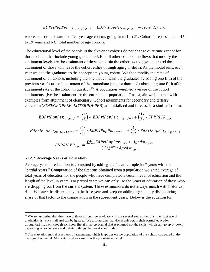
51
𝐸𝐷𝑃𝑟𝑖𝑃𝑜𝑝𝑃𝑒𝑟𝑐=5 𝑡𝑜 21,𝑝,𝑟,𝑡=1 = 𝐸𝐷𝑃𝑟𝑖𝑃𝑜𝑝𝑃𝑒𝑟𝑐−1,𝑝,𝑟,𝑡=1 − 𝑠𝑝𝑟𝑒𝑎𝑑𝑓𝑎𝑐𝑡𝑜𝑟
where, subscript c stand for five-year age cohorts going from 1 to 21. Cohort 4, represents the 15
to 19 years and NC, total number of age cohorts.
The educational level of the people in the five-year cohorts do not change over time except for
those cohorts that include young graduates15. For all other cohorts, the flows that modify the
attainment levels are the attainment of those who join the cohort as they get older and the
attainment of those who leave the cohort either through aging or death. As the model runs, each
year we add the graduates to the appropriate young cohort. We then modify the rates of
attainment of all cohorts including the one that contains the graduates by adding one fifth of the
previous year’s rate of attainment of the immediate junior cohort and subtracting one fifth of the
attainment rate of the cohort in question16. A population weighted average of the cohort
attainments give the attainment for the entire adult population. Once again we illustrate with
examples from attainment of elementary. Cohort attainments for secondary and tertiary
education (EDSECPOPPER, EDTERPOPPER) are initialized and forecast in a similar fashion.
𝐸𝐷𝑃𝑟𝑖𝑃𝑜𝑝𝑃𝑒𝑟𝑐=4,𝑝,𝑟,𝑡 = (4
5) ∗ 𝐸𝐷𝑃𝑟𝑖𝑃𝑜𝑝𝑃𝑒𝑟𝑐=4,𝑝,𝑟,𝑡−1 + (
1
5) ∗ 𝐸𝐷𝑃𝑅𝐼𝐶𝑅𝑟,𝑝,𝑡
𝐸𝑑𝑃𝑟𝑖𝑃𝑜𝑝𝑃𝑒𝑟𝑐=5 𝑡𝑜 21,𝑝,𝑟,𝑡 = (4
5) ∗ 𝐸𝑑𝑃𝑟𝑖𝑃𝑜𝑝𝑃𝑒𝑟𝑐,𝑝,𝑟,𝑡−1 + (
1
5) ∗ 𝐸𝑑𝑃𝑟𝑖𝑃𝑜𝑝𝑃𝑒𝑟𝑐−1,𝑝,𝑟,𝑡−1
𝐸𝐷𝑃𝑅𝐼𝑃𝐸𝑅𝑟,𝑝,𝑡 =∑ 𝐸𝑑𝑃𝑟𝑖𝑃𝑜𝑝𝑃𝑒𝑟𝑐,𝑝,𝑟,𝑡 ∗ 𝐴𝑔𝑒𝑑𝑠𝑡𝑐,𝑝,𝑟,𝑡
21𝑐=4
∑ 𝐴𝑔𝑒𝑑𝑠𝑡𝑐,𝑝,𝑟,𝑡𝑁𝐶𝑜ℎ𝑜𝑟𝑡𝑠𝑐=4
5.12.2 Average Years of Education
Average years of education is computed by adding the “level-completion” years with the
“partial-years.” Computation of the first one obtained from a population weighted average of
total years of education for the people who have completed a certain level of education and the
length of the level in years. For partial years we can only use the years of education of those who
are dropping out from the current system. These estimations do not always match with historical
data. We save the discrepancy in the base year and keep on adding a gradually disappearing
share of that factor to the computation in the subsequent years. Below is the equation for
15 We are assuming that the share of those among the graduate who are several years older than the right age of
graduation is very small and can be ignored. We also assume that the people retain their formal education
throughout life even though we know that it’s the credential that is retained not the skills, which can go up or down
depending on experience and training, things that we do not model.
16 The education model uses rates of attainment, which it applies on the population of the cohort, computed in the
demographic model. Mortality is taken care of in the population model.

52
computing average years using elementary education as an example (edprilen r,t is the duration
of primary cycle in years).
𝐴𝑣𝑔𝑌𝑒𝑎𝑟𝑠𝑃𝑟𝑖𝐸𝑑𝑃𝑜𝑝𝑝,𝑟,𝑡 = ∑ 𝐸𝐷𝑃𝑟𝑖𝑃𝑜𝑝𝑃𝑒𝑟𝑐,𝑝,𝑟,𝑡
100 ∗𝒆𝒅𝒑𝒓𝒊𝒍𝒆𝒏𝑟∗𝐴𝐺𝐸𝐷𝑆𝑇𝑐,𝑝,𝑟,𝑡𝑁𝐶𝑜ℎ𝑜𝑟𝑡𝑠𝑐=4
∑ 𝐴𝑔𝑒𝐷𝑠𝑡𝑐,𝑝,𝑟,𝑡𝑁𝐶𝑜ℎ𝑜𝑟𝑡𝑠𝑐=4
For those who dropout before completing a certain level we need to calculate the partial
attainment and add that to the average years of education. The average of the partial years of
education at a particular year is calculated from dropouts by level and grade as shown below.
Calculation of the average of partial years resulting from dropouts in primary education is
illustrated in the equations below. Partial years from current year dropouts at other levels of
education are calculated in the same manner and all the partial years are averaged to an overall
average. This new partial attainment is then added to the partial attainment of five year cohorts
which are initialized and advanced in a similar manner as that used for cohort averages on
completed attainment.
𝐷𝑟𝑜𝑝𝑜𝑢𝑡𝑅𝑎𝑡𝑒𝑝,𝑟,𝑡 = f(𝐸𝐷𝑃𝑅𝐼𝑆𝑈𝑅𝑝,𝑟,𝑡 , 𝒆𝒅𝒑𝒓𝒊𝒍𝒆𝒏𝑟)
𝐺𝑟_𝑆𝑡𝑢𝑑𝑒𝑛𝑡𝑠𝑑,𝑝,𝑟,𝑡 = 𝑓(𝐸𝐷𝑃𝑅𝐼𝐼𝑁𝑇𝑔,𝑟,𝑡 , 𝐷𝑟𝑜𝑝𝑜𝑢𝑡𝑅𝑎𝑡𝑒𝑔,𝑟,𝑡 , 𝒆𝒅𝒑𝒓𝒊𝒍𝒆𝒏𝑟)
𝑃𝑎𝑟𝑡𝑖𝑎𝑙𝑃𝑟𝑖𝑃𝑒𝑟𝑠𝑌𝑒𝑎𝑟𝑠𝑁𝑒𝑤𝑝,𝑟,𝑡
=(∑ 𝐺𝑟_𝑆𝑡𝑢𝑑𝑒𝑛𝑡𝑠𝑑,𝑝,𝑟,𝑡
𝒆𝒅𝒑𝒓𝒊𝒍𝒆𝒏𝑟𝑑=2 ∗ 𝐷𝑟𝑜𝑝𝑜𝑢𝑡𝑅𝑎𝑡𝑒𝑝,𝑟,𝑡 ∗ (𝑑 − 1)) ∗ ∑ 𝑓𝑎𝑔𝑒𝑑𝑠𝑡𝑐,𝑝,𝑟,𝑡
𝒆𝒅𝒑𝒓𝒊𝒍𝒆𝒏𝑟𝑐=𝒆𝒅𝒑𝒓𝒊𝒔𝒕𝒂𝒓𝒕𝑟
∑ 𝑓𝑎𝑔𝑒𝑑𝑠𝑡𝑐,𝑝,𝑟,𝑡𝒆𝒅𝒑𝒓𝒊𝒍𝒆𝒏𝑟𝑐=𝒆𝒅𝒑𝒓𝒊𝒔𝒕𝒂𝒓𝒕𝑟
Here, EDPRISUR is the survival rate in primary education, edpristart is the official entrance age
for primary schooling, Gr_Students is the enrollment at a certain grade, d is the grade counter
and fagedst is the population of the single year age cohort corresponding to the grade level.
Overall attainment, i.e., average years of education are calculated by averaging the attainments
and partial attainments of five year age cohorts as shown in the equation below. The suffixes on
the variables EDYRSAG15, EDYRSAG15TO24 and EDYRSAG25 indicate the age thresholds at
which or the age bracket over which attainment is averaged.
𝐸𝐷𝑌𝑅𝑆𝐴𝐺15𝑝,𝑟,𝑡
= 𝐴𝑣𝑔𝑌𝑒𝑎𝑟𝑠𝑃𝑟𝑖𝐸𝑑𝑃𝑜𝑝𝑝,𝑟,𝑡 + 𝐴𝑣𝑔𝑌𝑒𝑎𝑟𝑠𝑆𝑒𝑐𝐸𝑑𝑃𝑜𝑝𝑝,𝑟,𝑡
+ 𝐴𝑣𝑔𝑌𝑒𝑎𝑟𝑠𝑇𝑒𝑟𝐸𝑑𝑃𝑜𝑝𝑝,𝑟,𝑡 + 𝑃𝑎𝑟𝑡𝑖𝑎𝑙𝑌𝑒𝑎𝑟𝑠𝐸𝑑𝑃𝑜𝑝𝑝,𝑟,𝑡

53
5.12.3 Education Pyramids
Cohort attainments by level of education are used in to build a specialized educational attainment
display, commonly referred to as education pyramid in congruence with demographic pyramids
used to display population by age cohorts stacked one on top of the other with the men and
women cohorts put opposite to each other around a vertical axis. Education pyramid
superimposes educational attainment on top of the demographic pyramid.
6 Knowledge Systems
Knowledge and innovation are important drivers of economic growth and human well-being.
These activities also help societies address major social and environmental challenges. Education
and research and a linear relationship between these and product development are no longer
considered a good model of knowledge and innovation systems. However, the linear model was
380 304 228 152 76 0 76 152 228 304 380
100+ 95- 99 90- 94 85- 89 80- 84 75- 79 70- 74 65- 69 60- 64 55- 59 50- 54 45- 49 40- 44 35- 39 30- 34 25- 29 20- 24 15- 19 10- 14
5- 9 0- 4
Human Capital Distribution for World in Year 2015 [Base Case]
Male Millions Female
Children
No education or incomplete primary education
Completed primary education only
Completed through secondary education
Completed through tertiary education
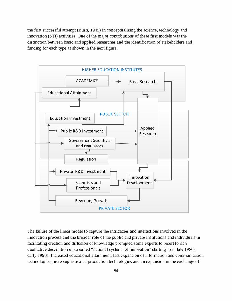
54
the first successful attempt (Bush, 1945) in conceptualizing the science, technology and
innovation (STI) activities. One of the major contributions of these first models was the
distinction between basic and applied researches and the identification of stakeholders and
funding for each type as shown in the next figure.
PUBLIC SECTOR
PRIVATE SECTOR
HIGHER EDUCATION INSTITUTES
Basic Research
Applied Research
InnovationDevelopment
ACADEMICS
Scientists and Professionals
Educational Attainment
Education Investment
Revenue, Growth
Public R&D Investment
Private R&D Investment
Government Scientists and regulators
Regulation
The failure of the linear model to capture the intricacies and interactions involved in the
innovation process and the broader role of the public and private institutions and individuals in
facilitating creation and diffusion of knowledge prompted some experts to resort to rich
qualitative description of so called “national systems of innovation” starting from late 1980s,
early 1990s. Increased educational attainment, fast expansion of information and communication
technologies, more sophisticated production technologies and an expansion in the exchange of
55
goods, ideas and people over the last few decades tell of something broader than just innovation
constrained within national boundaries. Recent literature17 use concepts like knowledge economy
or knowledge society to emphasize the recent proliferation of knowledge-intensive activities.
Another important phenomenon discussed in the literature is the systemic nature of the
knowledge and innovation and an interlinked emergence of major institutions within such a
system (Nelson Ed., 1993). Such a system, known today as the National Innovation System,
encompasses major actors, institutions and organizations involved in knowledge and innovation
activities and the linkages among them. From a policy perspective, the failures at one or more
components of the system, i.e., the systemic failures, justify policy actions more so than the
economic rational of market failure. The complementarity of the components of an innovation
system demands that the components be studied together. Accordingly, experts have come up
with composite indices for assessing the knowledge and innovation capacities of countries
around the world. Such indices give a good idea of the overall status of the innovation capacities
of the country and the stage of knowledge society it is in. The components of the composite
indices are categorized across four to five major dimensions or, pillars, as some studies call
these, for example, education and skills, information infrastructure, institutional regime, and
innovation activities are some of the pillars used by World Bank’s Knowledge Assessment
Methodologies (World Bank, 2007).
International Futures (IFs) Knowledge module builds on other knowledge systems measurement
approaches by designing a composite knowledge index (KNTOTALINDEX) comprised of five
sub-indices containing a total of (x) components. The indices and the sub-indices are then
forecast over the entire IFs’ horizon by combining the components which are themselves forecast
through different modules of the integrated IFs model. To our knowledge, IFs is the only model
capable of making such an organic forecast of the knowledge capacity of a country.
6.1 IFs Knowledge Indices:
The capacity of a society to tap from and add to the pool of existing knowledge, local and
global, depends on
- skills and qualifications of people to assimilate existing and new knowledge,
- an innovation system to facilitate development or adoption of of new knowledge,
processes and products
- a technological infrastructure to share, disseminate and regenerate knowledge and
information within and across societies
17 Peter Drucker popularized the term Knowledge Economy by using it as the title of a chapter in his book the Age
of Discontinuity. While the term can cover a wide array of activities the key characteristic of a knowledge economy
is a greater reliance on intellectual capabilities compared to that on physical inputs or natural resources (Powell and
Snellman, 2014).
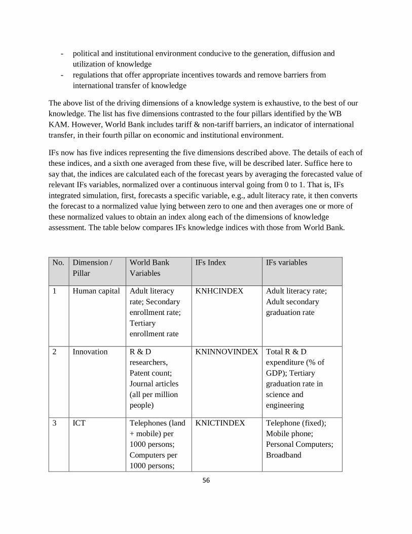
56
- political and institutional environment conducive to the generation, diffusion and
utilization of knowledge
- regulations that offer appropriate incentives towards and remove barriers from
international transfer of knowledge
The above list of the driving dimensions of a knowledge system is exhaustive, to the best of our
knowledge. The list has five dimensions contrasted to the four pillars identified by the WB
KAM. However, World Bank includes tariff & non-tariff barriers, an indicator of international
transfer, in their fourth pillar on economic and institutional environment.
IFs now has five indices representing the five dimensions described above. The details of each of
these indices, and a sixth one averaged from these five, will be described later. Suffice here to
say that, the indices are calculated each of the forecast years by averaging the forecasted value of
relevant IFs variables, normalized over a continuous interval going from 0 to 1. That is, IFs
integrated simulation, first, forecasts a specific variable, e.g., adult literacy rate, it then converts
the forecast to a normalized value lying between zero to one and then averages one or more of
these normalized values to obtain an index along each of the dimensions of knowledge
assessment. The table below compares IFs knowledge indices with those from World Bank.
No. Dimension /
Pillar
World Bank
Variables
IFs Index IFs variables
1 Human capital Adult literacy
rate; Secondary
enrollment rate;
Tertiary
enrollment rate
KNHCINDEX Adult literacy rate;
Adult secondary
graduation rate
2 Innovation R & D
researchers,
Patent count;
Journal articles
(all per million
people)
KNINNOVINDEX Total R & D
expenditure (% of
GDP); Tertiary
graduation rate in
science and
engineering
3 ICT Telephones (land
+ mobile) per
1000 persons;
Computers per
1000 persons;
KNICTINDEX Telephone (fixed);
Mobile phone;
Personal Computers;
Broadband
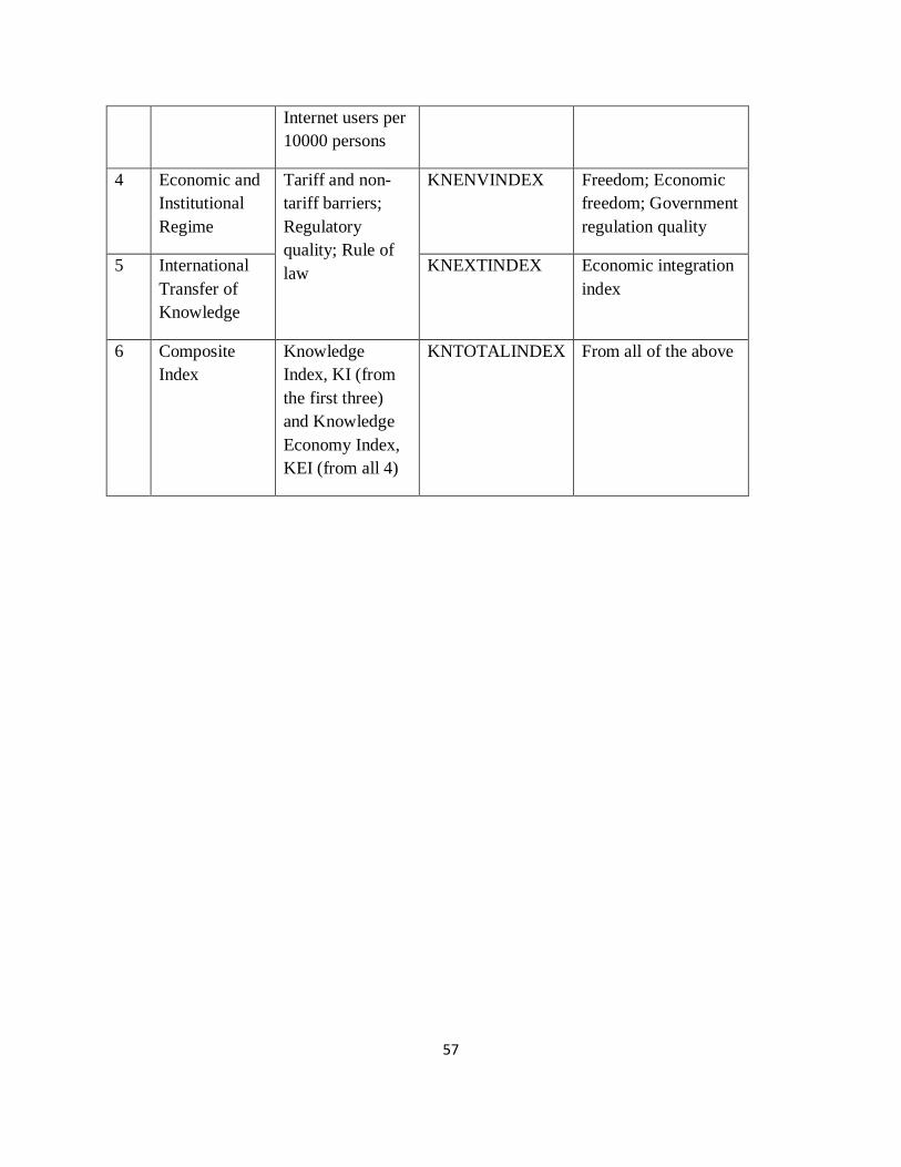
57
Internet users per
10000 persons
4 Economic and
Institutional
Regime
Tariff and non-
tariff barriers;
Regulatory
quality; Rule of
law
KNENVINDEX Freedom; Economic
freedom; Government
regulation quality
5 International
Transfer of
Knowledge
KNEXTINDEX Economic integration
index
6 Composite
Index
Knowledge
Index, KI (from
the first three)
and Knowledge
Economy Index,
KEI (from all 4)
KNTOTALINDEX From all of the above
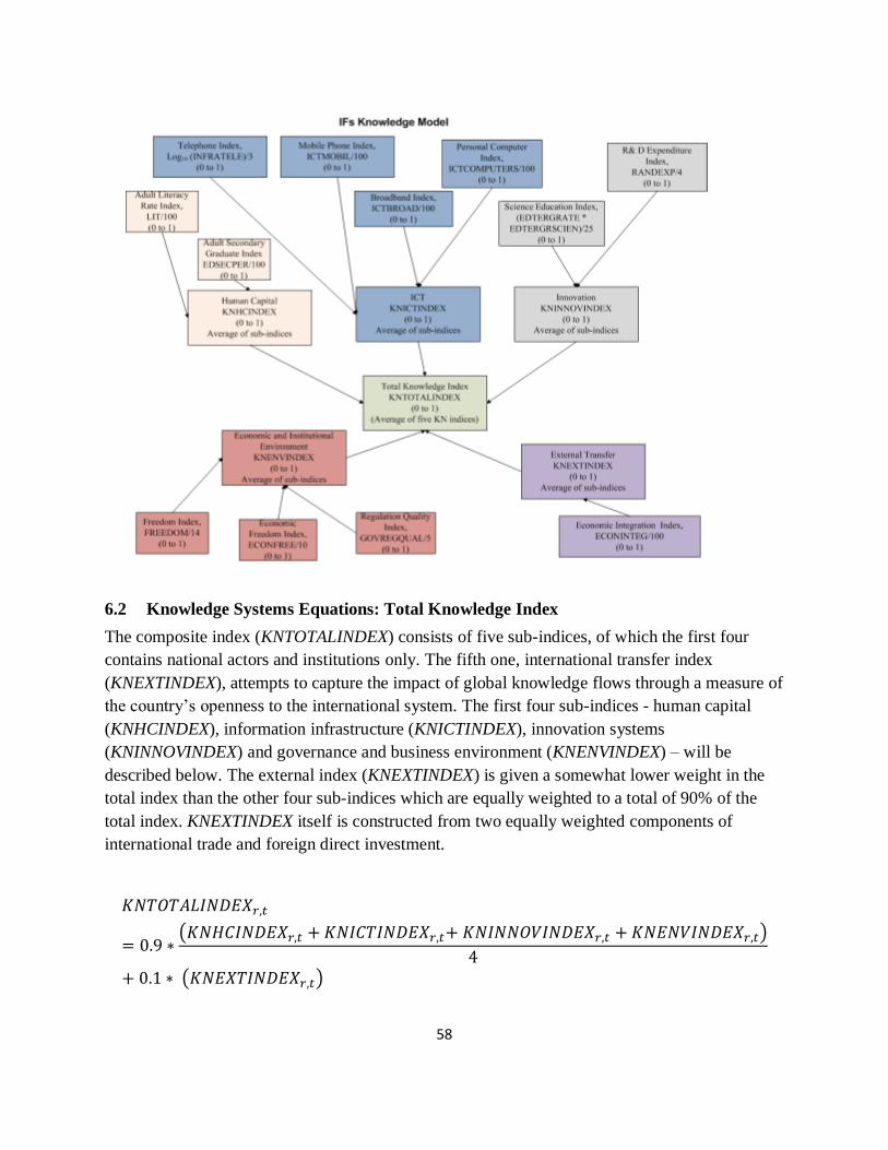
58
IFs Knowledge Model
6.2 Knowledge Systems Equations: Total Knowledge Index
The composite index (KNTOTALINDEX) consists of five sub-indices, of which the first four
contains national actors and institutions only. The fifth one, international transfer index
(KNEXTINDEX), attempts to capture the impact of global knowledge flows through a measure of
the country’s openness to the international system. The first four sub-indices - human capital
(KNHCINDEX), information infrastructure (KNICTINDEX), innovation systems
(KNINNOVINDEX) and governance and business environment (KNENVINDEX) – will be
described below. The external index (KNEXTINDEX) is given a somewhat lower weight in the
total index than the other four sub-indices which are equally weighted to a total of 90% of the
total index. KNEXTINDEX itself is constructed from two equally weighted components of
international trade and foreign direct investment.
𝐾𝑁𝑇𝑂𝑇𝐴𝐿𝐼𝑁𝐷𝐸𝑋𝑟,𝑡
= 0.9 ∗(𝐾𝑁𝐻𝐶𝐼𝑁𝐷𝐸𝑋𝑟,𝑡 + 𝐾𝑁𝐼𝐶𝑇𝐼𝑁𝐷𝐸𝑋𝑟,𝑡+ 𝐾𝑁𝐼𝑁𝑁𝑂𝑉𝐼𝑁𝐷𝐸𝑋𝑟,𝑡 + 𝐾𝑁𝐸𝑁𝑉𝐼𝑁𝐷𝐸𝑋𝑟,𝑡)
4+ 0.1 ∗ (𝐾𝑁𝐸𝑋𝑇𝐼𝑁𝐷𝐸𝑋𝑟,𝑡)
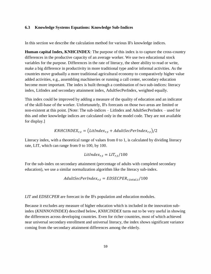
59
6.3 Knowledge Systems Equations: Knowledge Sub-Indices
In this section we describe the calculation method for various IFs knowledge indices.
Human capital Index, KNHCINDEX: The purpose of this index is to capture the cross-country
differences in the productive capacity of an average worker. We use two educational stock
variables for the purpose. Differences in the rate of literacy, the sheer ability to read or write,
make a big difference in productivity in more traditional type and/or informal activities. As the
countries move gradually a more traditional agricultural economy to comparatively higher value
added activities, e.g., assembling machineries or running a call center, secondary education
become more important. The index is built through a combination of two sub-indices: literacy
index, LitIndex and secondary attainment index, AdultSecPerIndex, weighted equally.
This index could be improved by adding a measure of the quality of education and an indicator
of the skill-base of the worker. Unfortunately, IFs forecasts on those two areas are limited or
non-existent at this point. [Note: The sub-indices – LitIndex and AdultSecPerIndex – used for
this and other knowledge indices are calculated only in the model code. They are not available
for display.]
𝐾𝑁𝐻𝐶𝐼𝑁𝐷𝐸𝑋𝑟,𝑡 = (𝐿𝑖𝑡𝐼𝑛𝑑𝑒𝑥𝑟,𝑡 + 𝐴𝑑𝑢𝑙𝑡𝑆𝑒𝑐𝑃𝑒𝑟𝐼𝑛𝑑𝑒𝑥𝑟,𝑡)/2
Literacy index, with a theoretical range of values from 0 to 1, is calculated by dividing literacy
rate, LIT, which can range from 0 to 100, by 100.
𝐿𝑖𝑡𝐼𝑛𝑑𝑒𝑥𝑟,𝑡 = 𝐿𝐼𝑇𝑟,𝑡/100
For the sub-index on secondary attainment (percentage of adults with completed secondary
education), we use a similar normalization algorithm like the literacy sub-index.
𝐴𝑑𝑢𝑙𝑡𝑆𝑒𝑐𝑃𝑒𝑟𝐼𝑛𝑑𝑒𝑥𝑟,𝑡 = 𝐸𝐷𝑆𝐸𝐶𝑃𝐸𝑅𝑟,𝑡𝑜𝑡𝑎𝑙,𝑡/100
LIT and EDSECPER are forecast in the IFs population and education modules.
Because it excludes any measure of higher education which is included in the innovation sub-
index (KNINNOVINDEX) described below, KNHCINDEX turns out to be very useful in showing
the differences across developing countries. Even for richer countries, most of which achieved
near universal secondary enrollment and universal literacy, the index shows significant variance
coming from the secondary attainment differences among the elderly.
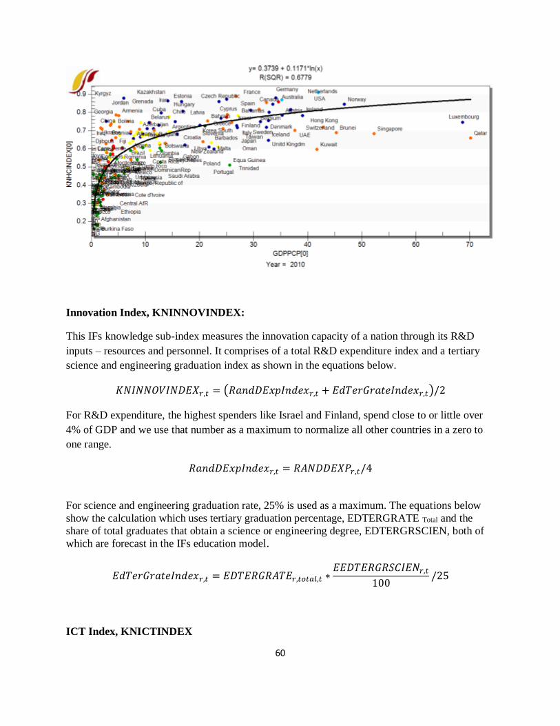
60
Innovation Index, KNINNOVINDEX:
This IFs knowledge sub-index measures the innovation capacity of a nation through its R&D
inputs – resources and personnel. It comprises of a total R&D expenditure index and a tertiary
science and engineering graduation index as shown in the equations below.
𝐾𝑁𝐼𝑁𝑁𝑂𝑉𝐼𝑁𝐷𝐸𝑋𝑟,𝑡 = (𝑅𝑎𝑛𝑑𝐷𝐸𝑥𝑝𝐼𝑛𝑑𝑒𝑥𝑟,𝑡 + 𝐸𝑑𝑇𝑒𝑟𝐺𝑟𝑎𝑡𝑒𝐼𝑛𝑑𝑒𝑥𝑟,𝑡)/2
For R&D expenditure, the highest spenders like Israel and Finland, spend close to or little over
4% of GDP and we use that number as a maximum to normalize all other countries in a zero to
one range.
𝑅𝑎𝑛𝑑𝐷𝐸𝑥𝑝𝐼𝑛𝑑𝑒𝑥𝑟,𝑡 = 𝑅𝐴𝑁𝐷𝐷𝐸𝑋𝑃𝑟,𝑡/4
For science and engineering graduation rate, 25% is used as a maximum. The equations below
show the calculation which uses tertiary graduation percentage, EDTERGRATE Total and the
share of total graduates that obtain a science or engineering degree, EDTERGRSCIEN, both of
which are forecast in the IFs education model.
𝐸𝑑𝑇𝑒𝑟𝐺𝑟𝑎𝑡𝑒𝐼𝑛𝑑𝑒𝑥𝑟,𝑡 = 𝐸𝐷𝑇𝐸𝑅𝐺𝑅𝐴𝑇𝐸𝑟,𝑡𝑜𝑡𝑎𝑙,𝑡 ∗𝐸𝐸𝐷𝑇𝐸𝑅𝐺𝑅𝑆𝐶𝐼𝐸𝑁𝑟,𝑡
100/25
ICT Index, KNICTINDEX
61
Information and communication technologies (ICT) have a very significant role in facilitating the
creation and diffusion of knowledge. IFs knowledge sub-index on ICT is built from the diffusion
rates of core ICT technologies mobile, landline, broadband and a personal computer access rate
sub-index. The telephone lines (fixed lines) sub-index, unlike the other three, use the logarithm
of telephone line access rates as the differences in impacts of plain old telephone system
decreases at higher access rates. In fact, the gradual shift from a wired to a wireless line as a
personal communication device, demands that we reconsider the inclusion of this component in
the ICT index.
𝐾𝑁𝐼𝐶𝑇𝐼𝑁𝐷𝐸𝑋𝑟,𝑡
= (𝐼𝐶𝑇𝑇𝑒𝑙𝑒𝑝ℎ𝑜𝑛𝑒𝐼𝑛𝑑𝑒𝑥𝑟,𝑡 + 𝐼𝐶𝑇𝑀𝑜𝑏𝑖𝑙𝑒𝐼𝑛𝑑𝑒𝑥𝑟,𝑡+ 𝐼𝐶𝑇𝐵𝑟𝑜𝑎𝑑𝐼𝑛𝑑𝑒𝑥𝑟,𝑡
+ 𝐼𝐶𝑇𝐶𝑜𝑚𝑝𝑢𝑡𝑒𝑟𝑠𝐼𝑛𝑑𝑒𝑥𝑟,𝑡)/4
𝐼𝐶𝑇𝑇𝑒𝑙𝑒𝑝ℎ𝑜𝑛𝑒𝐼𝑛𝑑𝑒𝑥𝑟,𝑡 = 𝑙𝑜𝑔(𝐼𝑁𝐹𝑅𝐴𝑇𝐸𝐿𝐸𝑟,𝑡) /3
𝐼𝐶𝑇𝑀𝑜𝑏𝑖𝑙𝑒𝐼𝑛𝑑𝑒𝑥𝑟,𝑡 = 𝐼𝐶𝑇𝑀𝑂𝐵𝐼𝐿𝑟,𝑡/100
𝐼𝐶𝑇𝐵𝑟𝑜𝑎𝑑𝐼𝑛𝑑𝑒𝑥𝑟,𝑡 = 𝐼𝐶𝑇𝐵𝑅𝑂𝐴𝐷𝑟,𝑡/100
𝐼𝐶𝑇𝐶𝑜𝑚𝑝𝑢𝑡𝑒𝑟𝑠𝐼𝑛𝑑𝑒𝑥𝑟,𝑡 = 𝐼𝐶𝑇𝐶𝑂𝑀𝑃𝑈𝑇𝐸𝑅𝑆𝑟,𝑡/100
Governance and Regulatory Environment, KNENVINDEX:
The existence of economic and regulatory institutions and an effective governance of such
institutions are important for generation, diffusion and utilization of knowledge. IFs knowledge
sub-index representing these, KNENVINDEX, is calculated from three sub-indices which are
themselves indices forecast by other IFs modules. These indices, one for economic freedom, a
second one for overall freedom in the society and a third one on governance regulatory quality
are each normalized to a 0 to 1 scale and averaged to get KNENVINDEX.
for the variables economic freedom, political freedom and governance regulation quality and
average them to KNENVINDEX.
𝐾𝑁𝐸𝑁𝑉𝐼𝑁𝐷𝐸𝑋𝑟,𝑡 = (𝐸𝑐𝑜𝑛𝐹𝑟𝑒𝑒𝐼𝑛𝑑𝑒𝑥𝑟,𝑡 + 𝐹𝑟𝑒𝑒𝐷𝑜𝑚𝐼𝑛𝑑𝑒𝑥𝑟,𝑡+ 𝐺𝑜𝑣𝑅𝑒𝑔𝑄𝑢𝑎𝑙𝐼𝑛𝑑𝑒𝑥𝑟,𝑡)/3
𝐸𝑐𝑜𝑛𝐹𝑟𝑒𝑒𝐼𝑛𝑑𝑒𝑥𝑟,𝑡 = 𝐸𝐶𝑂𝑁𝐹𝑅𝐸𝐸𝑟,𝑡/10
𝐹𝑟𝑒𝑒𝐷𝑜𝑚𝐼𝑛𝑑𝑒𝑥𝑟,𝑡 = 𝐹𝑅𝐸𝐸𝐷𝑂𝑀𝑟,𝑡/14
𝐺𝑜𝑣𝑅𝑒𝑔𝑄𝑢𝑎𝑙𝐼𝑛𝑑𝑒𝑥𝑟,𝑡 = 𝐺𝑂𝑉𝑅𝐸𝐺𝑄𝑈𝐴𝐿𝑟,𝑡/5
62
International Transfer Index, KNEXTINDEX
KNEXTINDEX attempts to represent cross-national knowledge flows, a major phenomenon in
today’s globalized world. The more open a country is the more likely it is for her to learn from
the global advancements in science, technology and other forms of knowledge. The sub-index
that IFs calculates uses two indicators, trade and foreign direct investment (FDI). FDI indicator is
given twice the weight given to trade volume.
𝐾𝑁𝐸𝑋𝑇𝐼𝑁𝐷𝐸𝑋𝑟,𝑡 = (𝑇𝑟𝑎𝑑𝑒𝐼𝑛𝑑𝑒𝑥𝑟,𝑡 + 2 ∗ 𝐼𝑛𝑣𝐼𝑛𝑑𝑒𝑥𝑟,𝑡)/2
𝑇𝑟𝑎𝑑𝑒𝐼𝑛𝑑𝑒𝑥𝑟,𝑡 = 𝑙𝑜𝑔𝑋𝑅𝑃𝐴𝑟,𝑡 + 𝑀𝑅𝑃𝐴𝑟,𝑡
𝐺𝐷𝑃𝑃𝑂𝑇𝑟,𝑡/ 𝑙𝑜𝑔 1000
𝐼𝑛𝑣𝐼𝑛𝑑𝑒𝑥𝑟,𝑡 = 𝑙𝑜𝑔𝑋𝐹𝐷𝐼𝑆𝑇𝑂𝐶𝐾𝑟,𝑡 + 𝑋𝐹𝐷𝐼𝑆𝑇𝑂𝑈𝑇𝑟,𝑡
𝐺𝐷𝑃𝑃𝑂𝑇𝑟,𝑡/ 𝑙𝑜𝑔 500
7 Reference
Archibugi, Daniele, and Alberto Coco. 2005. “Measuring Technological Capabilities at the
Country Level: A Survey and a Menu for Choice.” Research Policy 34(2). Research
Policy: 175–194.
Bush, Vannevar. 1945. Science: The Endless Frontier. Washington: United States Government
Printing Office.
Barro, Robert J. and Jong-Wha Lee. 2015. Education Matters: Global Schooling Gains from the
19th to the 21st Century. Oxford University Press, NY.
Barro, Robert and Jong-Wha Lee. 2013. "A New Data Set of Educational Attainment in the
World, 1950-2010." Journal of Development Economics. Volume 104, September 2013,
pp 184-198.
Bruns, Barbara, Alain Mingat, and Ramahatra Rakotomalala. 2003. Achieving Universal
Primary Education by 2015: A Chance for Every Child. Washington, DC: World Bank.
Chen, Derek H. C., and Carl J. Dahlman. 2005. The Knowledge Economy, the KAM
63
Methodology and World Bank Operations. The World Bank, October 19.
Clemens, Michael A. 2004. The Long Walk to School: International education goals in historical
perspective. Econ WPA, March. http://ideas.repec.org/p/wpa/wuwpdc/0403007.html.
Cohen, Daniel, and Marcelo Soto. 2001. “Growth and Human Capital: Good Data, Good
Results.” Technical Paper 179. Paris: OECD.
Cuaresma, Jesus Crespo, and Wolfgang Lutz. 2007 (April). “Human Capital, Age Structure and
Economic Growth: Evidence from a New Dataset.” Interim Report IR-07-011.
Laxenburg, Austria: International Institute for Applied Systems Analysis.
Delamonica, Enrique, Santosh Mehrotra, and Jan Vandemoortele. 2001 (August). “Is EFA
Affordable? Estimating the Global Minimum Cost of ‘Education for All’”. Innocenti
Working Paper No. 87. Florence: UNICEF Innocenti Research Centre.
http://ideas.repec.org/p/wpa/wuwpdc/0403007.html.
Dickson, Janet R., Barry B. Hughes, and Mohammod T. Irfan. 2010. Advancing Global
Education. Vol 2, Patterns of Potential Human Progress series. Boulder, CO, and New
Delhi, India: Paradigm Publishers and Oxford University Press.
http://www.ifs.du.edu/documents
Drucker, P. 1969. The Age of Discontinuity; Guidelines to Our changing Society. New York:
Harper and Row.
Dutta, Soumitra (Ed.). 2013. The Global Innovation Index 2013. The Local Dynamics of
Innovation.
Hughes, Barry B. 2004b (March). “International Futures (IFs): An Overview of Structural
Design.” Pardee Center for International Futures Working Paper, Denver, CO.
http://www.ifs.du.edu/documents/reports.aspx
Hughes, Barry B. and Evan E. Hillebrand. 2006. Exploring and Shaping International Futures.
Boulder, Co: Paradigm Publishers.
Hughes, Barry B. with Anwar Hossain and Mohammod T. Irfan. 2004 (May). “The Structure of
IFs.” Pardee Center for International Futures Working Paper, Denver, CO.
http://www.ifs.du.edu/documents/reports.aspx.
Irfan, Mohammod T. 2008. “A Global Education Transition: Computer Simulation of
Alternative Paths in Universal Basic Education,” Ph.D. dissertation presented to the Josef
64
Korbel School of International Studies, University of Denver, Denver, Colorado.
http://www.ifs.du.edu/documents/reports.aspx.
Juma, Calestous, and Lee Yee-Cheong. 2005. Innovation: Applying Knowledge in Development.
London: Earthscan. (Available online at
http://www.unmillenniumproject.org/documents/Science-complete.pdf)
KC, Samir, et. al. 2010. Projection of populations by level of educational attainment, age, and
sex for 120 countries for 2005-2050. DEMOGRAPHIC RESEARCH
Volume 22, Article 15, pages 383-472,
published 16 March 2010.
McMahon, Walter W. 1999 (first published in paperback in 2002). Education and Development:
Measuring the Social Benefits. Oxford: Oxford University Press.
Nelson, R. (ed.). 1993. National Innovation Systems. A Comparative Analysis, Oxford
University Press, New York/Oxford.
Powell WW and Snellman K. 2004. The Knowledge Economy. Annual Review of Sociology.
Vol. 30:199-220.
Wils, Annababette and Raymond O'Connor. 2003. “The causes and dynamics of the global
education transition.” AED Working Paper. Washington, DC: Academy for Educational
Development
UNESCO. 2010. UNESCO Science Report 2010. The Current Status of Science around the
World. UNESCO. Paris.
World Bank. 2010. Innovation Policy: A Guide for Developing Countries. (Available online at
https://openknowledge.worldbank.org/bitstream/handle/10986/2460/548930PUB0EPI11
C10Dislosed061312010.pdf?sequence=1
World Bank. 2007. Building Knowledge Economies: Advanced Strategies for Development.
WBI Development Studies. Washington, D.C: World Bank. (Available online at
http://siteresources.worldbank.org/KFDLP/Resources/461197-
1199907090464/BuildingKEbook.pdf

65