fractional order control of a e xible robot

Fractional order control of a flexible robot

Duarte Valerio1, and Jose Sa da Costa1

1Department of Mechanical Engineering, GCARTechnical University of Lisbon, Instituto Superior Tecnico, Lisbon, Portugal

{dvalerio,sadacosta}@dem.ist.utl.pt

Abstract — Low robot mass / carried mass ratios make flexible robots rather at-tractive from the energy saving point of view, but difficulties arising from its controlare significant, especially when high accuracy is needed. In this paper fractional or-der control for a two degree of mobility flexible robot is presented. Fractional orderPID controllers with parameters tuned using genetic algorithms ensure, in simula-tions, a good following of trajectories, unlike integer order PID controllers, clearlyless fit for such a task. Performances deteriorate in laboratory but still show frac-tional order control to be a promising option for this application.

1 IntroductionA robot is said to be flexible if designed in such a manner that its structure will undergodeformation (and consequently vibration) under normal operation conditions to such adegree that rigid body models become too poor for providing suitable approximations forcontrol. Low robot mass / carried mass ratios make flexible robots rather attractive fromthe energy saving point of view, but difficulties arising from its control are significant,especially for tasks demanding a high accuracy. In this paper fractional (or non-integer)order control for a flexible robot is presented. Fractional order control has been appliedwith success in rigid robots, both for position control and hybrid position-force control [1,2, 3], and in a one-degree of mobility flexible robot [4]. Whenever models with significantnon-linearities were used, parameter tuning was achieved either by trial and error [1] orby using a genetic algorithm [2, 3].

In what follows the application of fractional order control to a laboratory prototype ofa two-degrees of mobility flexible robot, achieving a stable control-loop for the positionof its tip, is described. Material is organised as follows. In section 2 a model of the robotis presented. In section 3 the implementation of fractional order controllers is addressedand genetic algorithms are shortly presented as an introduction to the genetic algorithmused in this particular case for tuning control parameters. In section 4 simulation andlaboratory results are presented. Some conclusions are drawn in section 5.

2 Flexible robot addressedThe flexible robot addressed in this paper is a two-degree of mobility planar horizontalrobot extant at the Control, Automation and Robotics Laboratory of the authors’ Univer-

VALERIO, SA DA COSTA

x

y

rigid link (inertia IR0, length LR)

flexible link (linear density ρ, Young modulus E, area moment of inertia I, length L)

rigid hub (mass mH, inertia IH, radius r)

lateral deviation v, beam shortening u

τ2

θ1

θ2

τ1

Figure 1: Flexible robotic arm addressed in this paper

sity. It consists of a rigid link and a flexible link, connected by rigid hubs, as seen inFigure 1. In each hub there are a motor, a tachometer and an encoder; the vibration ofthe flexible link is measured by means of two extensometer bridges. Control is performedusing Matlab’s xPC target toolbox. The robot’s tip position can be reckoned from the twoangles θ1 and θ2 and the elastic displacement of the flexible link v. A model of the robot,drawn from [5], is given in an Appendix.

3 Control of the robot

3.1 Fractional order controllers

Control of the position of the tip of the robot was attempted using both usual digital PIDcontrollers and digital fractional PID controllers. The former are the weighted sum of pro-portional, integral and derivative control actions. The later generalise this control structureby allowing differentiation and integration orders other than 1, all real numbers being ad-missible. Thus five parameters are needed to define a fractional PID: the proportional,integral and derivative gains, the differentiation order, and the integration order. There areseveral ways for reckoning a fractional derivative or integral of a sampled signal. The onechosen stems from Tustin’s formula for approximating a first order derivative, that will

FRACTIONAL ORDER CONTROL OF A FLEXIBLE ROBOT

have to be raised to the fractional order, which we will call ν:(

2

T

1− z−1

1 + z−1

)ν

(1)

Here T is the sampling time. Since this involves fractional powers of the delay operatorz−1, we expand (1) into a MacLaurin series and truncate it after some number of terms p.The result is [2, 6]

Dνf(t) ≈ f(t)p∑

i=0

z−ii∑

j=0

(−1)j(

2

T

)νΓ(ν + 1)Γ(−ν + 1)

Γ(ν − j + 1)Γ(j + 1)Γ(i− j + 1)Γ(−ν + j − i+ 1)(2)

Instead of beginning with Tustin formula, a first-order backward finite difference mighthave been used in (2). Or else the expected impulse response might have been used tofind the coefficients of the finite impulse response filter of equation (2). Or, instead ofa truncated MacLaurin series expansion, a truncated continued fraction expansion mighthave been used (resulting in an infinite response filter). [2, 4, 7] All these hypotheses havebeen tested, but the best results were obtained with (2), which was thus retained.

The control structure employed is that of Figure 2. Notice that v enters the control loopwith its signal changed. This is a way of dealing with the non-minimum phase behaviourof the plant that results from the flexibility of the second link: when it turns to one side,its tip bends to the other side in a first moment [8]. Vector T contains the torques andvector q contains angles θ1 and θ2 and the information obtained from the extensometers(see (16), (33), (34) and (35) in the Appendix).

Cartesian coordinates

Tq

vR ob ot

error control actionN on- integ er P I D

oru su al P I D

x , y

K inem atic equ ations

I nverse of

th e m atrix w ith th eJ acob ian of

k inem atic equ ations- 1

R ef erence

Figure 2: Control loop

3.2 Genetic algorithms

Since a genetic algorithm was successfully used in [3] for tuning the controller’s param-eters, this option was also adopted in this case. Genetic algorithms are an optimisationmethod useful in situations involving non-linearities and local minima, consisting essen-tially in a refined trial-and-error that imitates the evolutionary principle of the survival ofthe fittest [9].

The algorithm used for fitting fractional PIDs, implemented in Matlab, was as follows:

One: A population of 50 elements is created. Each corresponds to a set of two fractionalPIDs, the first (C1) for the first joint of the robot and the second (C2) for the second


0 0.5 1 1.5 2−0.1

0

0.1

0.2

0.3

0.4

0.5

0.6

time (s)

belo

w: y

(m);

abov

e: x

(m)

experimental reference

simulation

experimental

0.35 0.4 0.45 0.5 0.55 0.6 0.65−0.06

−0.04

−0.02

0

0.02

0.04

0.06

x (m)

y(m

)

experimental

simulation

experimental

ref.

0 0.5 1 1.5 2−0.05

0

0.05

time (s)

vibr

atio

n of

the

tip (m

)

experimental

simulation

Figure 3: Control results for a linear trajectory (reference trajectory dashed)

joint, given by

C1 = k1Dν1 + k2D

ν2 + k3 (3)C2 = k4D

ν4 + k5Dν5 + k6 (4)

Parameters, which will be stored as real numbers, are randomly chosen with normaldistributions with the means and standard deviations of Table 1, which are based onprevious trial-and-error tuning.

k1 ν1 k2 ν2 k3 k4 ν4 k5 ν5 k6

x 104 0 1 0 10−2 102 0 1 0 10−2

σx 2000 2 0.1 0.1 0.1 20 2 0.1 0.1 0.1

Table 1: Parameters’ distributions

Two: Following steps are performed until 100 iterations are reached, or until no improve-ment arises over 10 iterations.

Three: Control is simulated for all individuals. Fractional derivatives are approximatedby (2); the number of terms retained p was set to 10.

Four: A performance index is reckoned [3]. It includes the sum of the integrals of thesquares of the errors in both coordinates, and a term for penalising large vibrationsof the tip of the robot, since they are hard to deal with, and a potential source ofinaccuracy. Vibration at the end of the simulation should be as small as possible, so


0 0.5 1 1.5 2 2.5 3−0.1

0

0.1

0.2

0.3

0.4

0.5

time (s)

belo

w: y

(m);

abov

e: x

(m)

simulation experimental

0.25 0.3 0.35 0.4 0.45 0.5 0.55−0.1

−0.05

0

0.05

0.1

0.15

x (m)

y(m

)


reference


experimental

0 0.5 1 1.5 2 2.5 3−0.03

−0.02

−0.01

0

0.01

0.02

0.03

time (s)

vibr

atio

n of

the

tip (m

)

experimental

simulation

Figure 4: Control results for a two-loop trajectory (reference trajectory dashed)

that the robot may come to rest at the desired location; thus, as vibration cannot becompletely avoided, it is penalised increasingly with time:

I =∫ tend

0

[

(x− xref )2 + (y − yref )

2 + t2v4]

dt (5)

Five: Eliminate all individuals save those with the 6 best performance indexes. These areallowed into the next generation (this is called elitism), and are the only ones thatmay reproduce or mutate.

Six: One-half of the eliminated individuals are replaced by mutations of the survivingones. Mutants begin as copies of a randomly chosen survivor. The number of pa-rameters that mutate is randomly chosen; the probability decreases exponentiallywith the number of parameters, so that it will be more likely that few parameterswill change. The change consists in adding a Gaussianly distributed random num-ber with zero-mean and variance equal to one-tenth of the mutating parameter.

Seven: One-fourth of the eliminated individuals are replaced by descendents of the sur-viving ones. Each descendant is the offspring of two randomly chosen survivors;each of the ten parameters listed in Table 1 is drawn, randomly, from one of theparents. Each individual being thus split into ten pieces by nine cuts, this is callednine point cross-over [9].

Eight: One-fourth of the eliminated individuals are replaced by randomly generated indi-viduals, such as those of the original population—save that they are fewer in number.This is called spontaneous generation [3].


0 0.5 1 1.5 2 2.5 3−0.2

0

0.2

0.4

0.6

time (s)

belo

w: y

(m);

abov

e: x

(m)

0.25 0.3 0.35 0.4 0.45 0.5 0.55

−0.1

−0.05

0

0.05

0.1

0.15

x (m)

y(m

)


experimental

0 0.5 1 1.5 2 2.5 3−0.03

−0.02

−0.01

0

0.01

0.02

0.03

time (s)

vibr

atio

n of

the

tip (m

)

experimental simulation

Figure 5: Control results for a circular trajectory (reference trajectory dashed)

A similar algorithm was used for fitting PIDs to the robot. The distributions given inTable 1 for parameters k1, k2, k3, k4, k5 and k6 were used with this algorithm as well; ν1

and ν4 were forced to be 1; ν2 and ν5 were forced to be −1.

4 ResultsThree different trajectories were considered and different fractional PIDs were tuned foreach. Trajectories correspond to movements usually required from robots. Figure 3,Figure 4 and Figure 5 show, for each trajectory, how the position of the tip of the robotevolves with time, the trajectory it describes in space, and the vibration it undergoes. Bothsimulation and experimental results are shown. The sampling time was 1 ms; controllers’parameters are given in Table 2; since only once the two available fractional derivativeswere needed, the structure of the fractional PID seems to have been a reasonable choice.

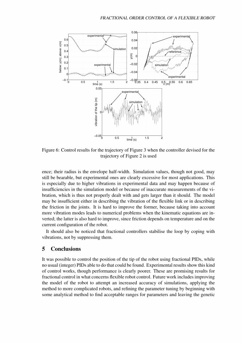
Whatever the trajectory, no integer PIDs were found that could stabilise the control-loop. This does not prove, of course, that the plant cannot be controlled with integerPIDs. But the fact that no such controllers were found, while acceptable fractional PIDswere, shows that the latter are clearly superior for this application. Furthermore, con-trollers developed for one trajectory also work for other references as well. An example(among others possible) is shown in Figure 6, showing that controllers work for trajecto-ries different from that they were devised for.

However, it is also clear from these results that the experimental performance is clearlyworse than what was expected from simulations. Table 3 gives the half-width of an en-velope around the reference trajectory that fully covers each simulation or experimentalresult. These envelopes are a set of circles centred on the successive points of the refer-


0 0.5 1 1.5 2−0.1

0

0.1

0.2

0.3

0.4

0.5

0.6

time (s)

belo

w: y

(m);

abov

e: x

(m)

experimental

simulation

experimental

0.35 0.4 0.45 0.5 0.55 0.6 0.65−0.06

−0.04

−0.02

0

0.02

0.04

0.06

x (m)

y(m

)

experimental

simulation

reference

experimental

0 0.5 1 1.5 2−0.05

0

0.05

time (s)

vibr

atio

n of

the

tip (m

)

simulation

experimental

Figure 6: Control results for the trajectory of Figure 3 when the controller devised for thetrajectory of Figure 2 is used

ence; their radius is the envelope half-width. Simulation values, though not good, maystill be bearable, but experimental ones are clearly excessive for most applications. Thisis especially due to higher vibrations in experimental data and may happen because ofinsufficiencies in the simulation model or because of inaccurate measurements of the vi-bration, which is thus not properly dealt with and gets larger than it should. The modelmay be insufficient either in describing the vibration of the flexible link or in describingthe friction in the joints. It is hard to improve the former, because taking into accountmore vibration modes leads to numerical problems when the kinematic equations are in-verted; the latter is also hard to improve, since friction depends on temperature and on thecurrent configuration of the robot.

It should also be noticed that fractional controllers stabilise the loop by coping withvibrations, not by suppressing them.

5 Conclusions

It was possible to control the position of the tip of the robot using fractional PIDs, whileno usual (integer) PIDs able to do that could be found. Experimental results show this kindof control works, though performance is clearly poorer. These are promising results forfractional control in what concerns flexible robot control. Future work includes improvingthe model of the robot to attempt an increased accuracy of simulations, applying themethod to more complicated robots, and refining the parameter tuning by beginning withsome analytical method to find acceptable ranges for parameters and leaving the genetic


Figure 3 Figure 4 Figure 5k1 4.81× 1014 3.89× 1014 59.4ν1 −3.63 −3.54 0.715k2 0 0 0ν2 — — —k3 0.0265 0.318 0.117k4 11.8 3.91× 103 304ν4 0.298 −0.498 −0.114k5 0 1.6106 0ν4 — 0.0101 —k6 0.0929 0.400 0.0121

Table 2: Controllers’ parameters

Simulation ExperimentalFigure 3 0.016 m 0.053 mFigure 4 0.014 m 0.021 mFigure 5 0.006 m 0.018 mFigure 6 0.033 m 0.042 m

Table 3: Half-width of the envelope of the reference containing simulated andexperimental control results

algorithm for fine-tuning only.

Appendix

Nomenclature used in the model of the robot:

C centrifugal and Coriolis vectorE Young modulus of the robot’s flexible linkF viscous friction coefficients vectorH mass matrixIb moment of inertia of the robot’s flexible linkIm1 moment of inertia of the motor of the rigid link’s jointIm2 moment of inertia of the motor of joint between the two linksIH moment of inertia of the hub connecting the linksIR0 moment of inertia of the robot’s rigid linkK stiffness matrixL length of the robot’s flexible linkLR length of the robot’s rigid linkM, N auxiliary matrixesM , S auxiliary functionsT vector with the torques applied


mb mass of the robot’s flexible link, equal to ρLmH mass of the hub connecting the linksq time-varying vector of the coordinates that define the robot’s stater radius of the hub connecting the linksr1 transmission relation of the rigid link’s jointr2 transmission relation of the joint between the two linksu beam shortening in the flexible link measured longitudinallyv elastic displacement (lateral deviation) of the flexible linkαij , γij , Φ auxiliary quantitiesβi eigenvalues corresponding to the free vibration modes of the robot’s flexible linkηi(t) weighing coefficients called elastic coordinatesθ1, θ2 angles of the linksρ linear density of the robot’s flexible linkτ1, τ2 torques applied at the joints by motorsχi normalised clamped-free vibration modes

The following auxiliary quantities will be used:

Mi,j =∫ r+L

rM (x)

dχi (x)

dx

dχj (x)

dxdx (6)

Ni,j =∫ r+L

rS (x)

dχi (x)

dx

dχj (x)

dxdx (7)

M (x) =∫ r+L

xρdξ (8)

S (x) =∫ r+L

xρξdξ (9)

γij =∫ r+L

rS (x)χi (x)

d2χj (x)

dx2dx (10)

γ′ij =∫ r+L

r

dS (x)

dxχi (x)

dχj (x)

dxdx (11)

αij =∫ r+L

rM (x)χi (x)

d2χj (x)

dx2dx (12)

α′ij =∫ r+L

r

dM (x)

dxχi (x)

dχj (x)

dxdx (13)

Φ (i) =∫ r+L

rχi (x) dx (14)

χi (x) = cosh [βi (x− r)]− cos [βi (x− r)]

−cosh (βiL) + cos (βiL)

sinh (βiL) + sin (βiL){sinh [βi (x− r)]− sin [βi (x− r)]} (15)

Beam shortening u was neglected; elastic displacement v was approximated by a finiteseries

v (x, t) =n∑

i=1

χi (x) ηi (t) (16)


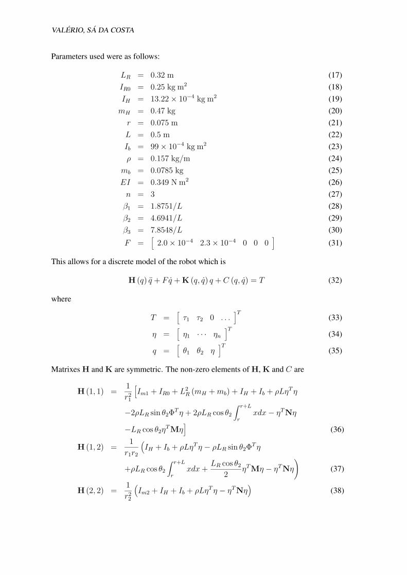
Parameters used were as follows:

LR = 0.32 m (17)IR0 = 0.25 kg m2 (18)IH = 13.22× 10−4 kg m2 (19)mH = 0.47 kg (20)r = 0.075 m (21)L = 0.5 m (22)Ib = 99× 10−4 kg m2 (23)ρ = 0.157 kg/m (24)

mb = 0.0785 kg (25)EI = 0.349 N m2 (26)n = 3 (27)β1 = 1.8751/L (28)β2 = 4.6941/L (29)β3 = 7.8548/L (30)

F =[

2.0× 10−4 2.3× 10−4 0 0 0]

(31)

This allows for a discrete model of the robot which is

H (q) q + F q + K (q, q) q + C (q, q) = T (32)

where

T =[

τ1 τ2 0 . . .]T

(33)

η =[

η1 · · · ηn]T

(34)

q =[

θ1 θ2 η]T

(35)

Matrixes H and K are symmetric. The non-zero elements of H, K and C are

H (1, 1) =1

r21

[

Im1 + IR0 + L2

R (mH +mb) + IH + Ib + ρLηTη

−2ρLR sin θ2ΦTη + 2ρLR cos θ2

∫ r+L

rxdx− ηTNη

−LR cos θ2ηTMη

]

(36)

H (1, 2) =1

r1r2

(

IH + Ib + ρLηTη − ρLR sin θ2ΦTη

+ρLR cos θ2

∫ r+L

rxdx+

LR cos θ2

2ηTMη − ηTNη

)

(37)

H (2, 2) =1

r22

(

Im2 + IH + Ib + ρLηTη − ηTNη)

(38)


H (1, j) =1

r1

(

ρ∫ r+L

rxχj−2 (x) dx

+LR cos θ2ρ∫ r+L

rχj−2 (x) dx

)

, 3 ≤ j ≤ n (39)

H (2, j) =1

r2

(

ρ∫ r+L

rxχj−2 (x) dx

)

, 3 ≤ j ≤ n (40)

H (3, j) = ρL, 3 ≤ j ≤ n (41)K (i+ 2, i+ 2) = EILβ4

i − θ2

1 [ρL+ γii + γ′ii + LR cos θ2 (αii + α′ii)]

−θ2

2 (ρL+ γii + γ′ii)

−2θ1θ2

[

ρL+ γii + γ′ii +LR cos θ2

2(αii + α′ii)

]

,

1 ≤ i ≤ n (42)K (i+ 2, j + 2) = −θ2

1 [γii + γ′ii + LR cos θ2 (αii + α′ii)]

−θ2

2 (γii + γ′ii)− 2θ1θ2

[

γii + γ′ii +LR cos θ2

2(αii + α′ii)

]

,

1 ≤ i ≤ n ∧ 1 ≤ j ≤ n ∧ i 6= j (43)

C (1) =1

r1

[(

ρLηT − ρLR sin θ2ΦT − ηTN− LR cos θ2η

TM

)

2θ1η

+

(

ρLηT − ρLR sin θ2ΦT − ηTN +

LR cos θ2

2ηTM

)

2θ2η

+

(

−ρLR sin θ2

∫ r+L

rxdx−

LR sin θ2

2ηTMη

−ρLR cos θ2ΦTη)

θ2

2 +

(

−ρLR sin θ2

∫ r+L

rxdx

+LR sin θ2

2ηTMη − ρLR cos θ2Φ

Tη

)

2θ1θ2

]

(44)

C (2) =1

r2

[(

ρLηT +LR cos θ2

2ηTM− ηTN

)

2θ1η

+

(

ρLR sin θ2

∫ r+L

rxdx+ ρLR cos θ2Φ

Tη −LR sin θ2

2ηTMη

)

θ2

1

+(

ρLηT − ηTN)

2ηθ2 − θ1θ2LR sin θ2ηTMη

]

(45)

C (i) = θ1LR sin θ2ρ∫ r+L

rχi−2 (x) dx, 3 ≤ i ≤ n (46)

Beyond vector F , friction in the joints was modelled by means of a dead zone and ofCoulomb and viscous friction affecting the input of each:

τeffective = sign (τ) (µ |τ |+ τ0) (47)

Parameters are given in Table 4. These (as well as those of vector F given in (31))were found by minimising, using a genetic algorithm, the quadratic error of the modelresponses to steps and impulses.


First joint Second jointDead zone

[

−3.2379 2.9129]

Nm[

−0.5543 0.6608]

Nm

τ0 4.56 N m 0 N mµ 0.2585 1.0231

Table 4: Friction parameters

AcknowledgmentsDuarte Valerio was partially supported by programme POCTI, FCT, Ministerio da Ciencia e Tec-nologia, Portugal, grant number SFRH/BD/2875/2000, and ESF through the III Quadro Comu-nitario de Apoio. Both authors deeply appreciate significant support with the experimental setupprovided by Jorge Martins and Joao Reis.

References[1] J. A. T. Machado and A. Azenha. Fractional-order hybrid control of robot manipulators. In Pro-

ceedings of IEEE International Conference on Systems, Man and Cybernetics, pages 788–793. IEEE,1998.

[2] D. Valerio and J. Sa da Costa. Digital implementation of non-integer control and its application to atwo-link robotic arm. In European Control Conference, Cambridge, 2003.

[3] D. Valerio and J. Sa da Costa. Optimisation of non-integer order control parameters for a robotic arm.In 11th International Conference on Advanced Robotics, Coimbra, 2003.

[4] B. M. Vinagre. Modelado y control de sistemas dinamicos caracterizados por ecuaciones ıntegro-diferenciales de orden fraccional. PhD thesis, Universidad Nacional de Educacion a Distancia, Madrid,2001.

[5] J. Martins, M. Ayala Botto, and J. Sa da Costa. Modeling of flexible beams for robotic manipulators.Multibody system dynamics, 7:79–100, 2002.

[6] D. Valerio and J. Sa da Costa. Time domain implementations of non-integer order controllers. In 5thPortuguese Conference on Automatic Control, Aveiro, 2002. APCA.

[7] B. M. Vinagre, I. Podlubny, A. Hernndez, and V. Feliu. Some approximations of fractional orderoperators used in control theory and applications. Fractional Calculus & Applied analysis, 3:231–248,2000.

[8] M. Benosman, F. Boyer, G. Le Vey, and D. Primault. Flexible links manipulators: from modelling tocontrol. Journal of Intelligent and Robotic Systems, 34:381–414, 2002.

[9] J.-S. R. Jang. Derivative-free optimization. In Neuro-fuzzy and Soft Computing, pages 173–196.Prentice Hall, Upper Saddle River, 1997.

About the AuthorsDuarte Valerio received a Graduation and a Master’s degree in Mechanical Engineering from theTechnical University of Lisbon in 1999 and 2001. He is finishing a thesis for a doctoral degreeon the application of fractional calculus to control. His research interests include software forfractional control and the extraction of electrical energy from sea-waves.

Jose Sa da Costa is head of the Centre of Intelligent Systems and Professor in the MechanicalEngineering Department at the Technical University of Lisbon. His main interests in research andteaching are in the area of systems and control.

fractional order control of a e xible robot

Documents