four-chamber heart modeling and automatic …comaniciu.net/papers/heartmodeling_tmi08.pdf ·...

IEEE TRANSACTIONS ON MEDICAL IMAGING 1

Four-Chamber Heart Modeling and AutomaticSegmentation for 3D Cardiac CT Volumes UsingMarginal Space Learning and Steerable Features

Yefeng Zheng, Adrian Barbu, Bogdan Georgescu, Michael Scheuering, and Dorin Comaniciu

Abstract— We propose an automatic four-chamber heart seg-mentation system for the quantitative functional analysis ofthe heart from cardiac computed tomography (CT) volumes.Two topics are discussed: heart modeling and automatic modelfitting to an unseen volume. Heart modeling is a non-trivial tasksince the heart is a complex nonrigid organ. The model mustbe anatomically accurate, allow manual editing, and providesufficient information to guide automatic detection and segmen-tation. Unlike previous work, we explicitly represent importantlandmarks (such as the valves and the ventricular septum cusps)among the control points of the model. The control points canbe detected reliably to guide the automatic model fitting process.

Using this model, we develop an efficient and robust approachfor automatic heart chamber segmentation in 3D CT volumes.We formulate the segmentation as a two-step learning problem:anatomical structure localization and boundary delineation. Inboth steps, we exploit the recent advances in learning discrimina-tive models. A novel algorithm, marginal space learning (MSL),is introduced to solve the 9-dimensional similarity transforma-tion search problem for localizing the heart chambers. Afterdetermining the pose of the heart chambers, we estimate the3D shape through learning-based boundary delineation. Theproposed method has been extensively tested on the largestdataset (with 323 volumes from 137 patients) ever reported inthe literature. To the best of our knowledge, our system is thefastest with a speed of 4.0 seconds per volume (on a dual-core3.2 GHz processor) for the automatic segmentation of all fourchambers.

Index Terms— Heart modeling, heart segmentation, 3D objectdetection, marginal space learning

I. INTRODUCTION

Compared with other imaging modalities (such as ultra-sound and magnetic resonance imaging), cardiac computedtomography (CT) can provide detailed anatomic informationabout the heart chambers, large vessels, and coronary arter-ies [1]. Therefore, CT is an important imaging modality fordiagnosing cardiovascular diseases. Complete segmentation ofall four heart chambers, as shown in Fig. 1, is a prerequisitefor clinical investigations, providing critical information for

Manuscript received Oct. 8, 2007; revised July 10, 2008; accepted July 11,2008. Y. Zheng, B. Georgescu, and D. Comaniciu are with the Integrated DataSystems Department at Siemens Corporate Research, Princeton, NJ, USA. A.Barbu is with the School of Computational Science, Florida State University,Florida, USA. M. Scheuering is with the Computed Tomography Division,Siemens Healthcare, Forchheim, Germany.

A. Bardu contributed to this work while he was with Siemens CorporateResearch.

Copyright (c) 2008 IEEE. Personal use of this material is permitted.However, permission to use this material for any other purposes must beobtained from the IEEE by sending a request to [email protected].

quantitative functional analysis for the whole heart [2], [3].In this paper, we propose an automatic 3D heart chambersegmentation system using a surface-based four-chamber heartmodel. There are two major tasks to develop such an automaticsegmentation system: heart modeling (shape representation)and automatic model fitting (detection and segmentation). Dueto the complexity of cardiac anatomy, it is not trivial to repre-sent the anatomy accurately while keeping the model simpleenough for automatic segmentation and manual correction ifnecessary. The proposed heart model, as shown in Fig. 1 hasthe following advantages.

1) The heart valves are explicitly modeled as closed con-tours along their borders in our model. Therefore, ourmodel is more accurate concerning the anatomy, com-pared to previous closed-surface mesh models [4]–[6].

2) Important landmarks (e.g., valves and ventricular septumcusps) are explicitly represented in our model as controlpoints1. These landmarks can be detected reliably toguide the automatic model fitting process.

3) Our model is flexible. Chambers are coupled at atrioven-tricular valves and it is easy to extract each chamberfrom the whole heart model.

4) The proposed model is expandable. Our current workfocuses on the addition of extra elements, such asdynamic valve modules [7].

5) We propose two approaches to enforce the mesh pointcorrespondence, namely the rotation-axis based andparallel-slice based methods. With such built-in cor-respondence, we can easily learn a statistical shapemodel [8] to enforce shape constraints in our automaticmodel fitting approach.

Using the proposed heart model, we present an automaticheart segmentation method based on machine learning toexploit a large database of annotated CT volumes. As shown inFig. 2, the segmentation procedure has two stages: automaticheart localization and control point guided nonrigid deforma-tion estimation. Automatic heart localization is largely ignoredin early work on heart segmentation [9]–[12]. Recently, learn-ing based approaches have been successfully demonstrated onmany 2D object detection problems [13], [14]. However, thereare two challenges in applying these techniques to 3D objectdetection: 1) the exponential computation demands by the useof exhaustive search and 2) lack of efficient features that can

1“Landmark” is a term used in relation with the anatomy and a “controlpoint” is a mesh point, representing the corresponding landmark in the mesh.


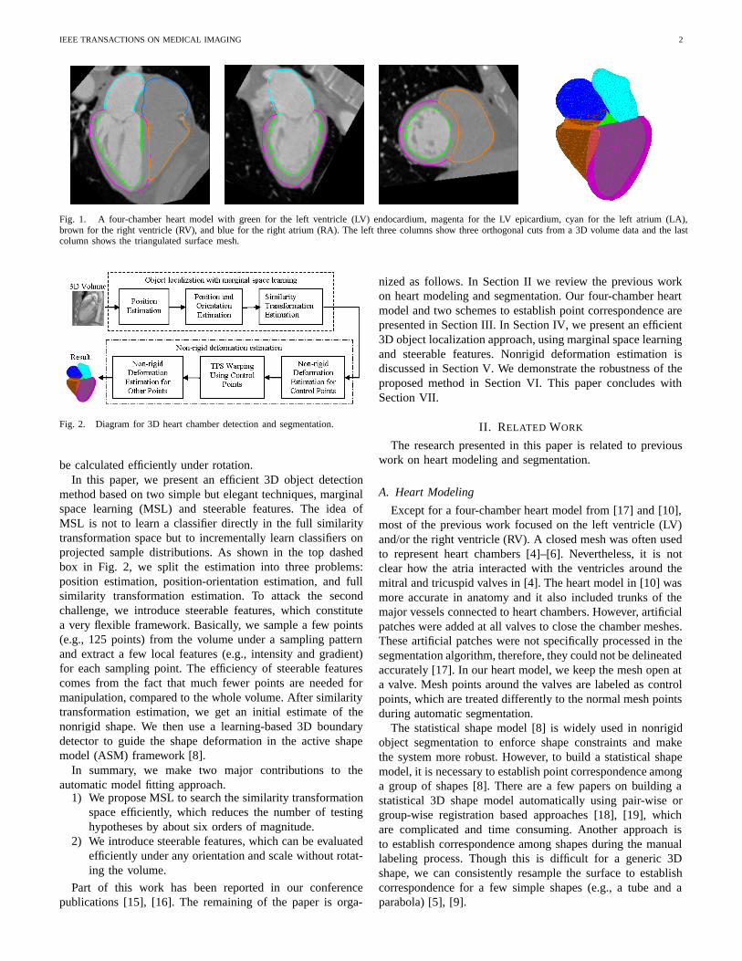
Fig. 1. A four-chamber heart model with green for the left ventricle (LV) endocardium, magenta for the LV epicardium, cyan for the left atrium (LA),brown for the right ventricle (RV), and blue for the right atrium (RA). The left three columns show three orthogonal cuts from a 3D volume data and the lastcolumn shows the triangulated surface mesh.

Fig. 2. Diagram for 3D heart chamber detection and segmentation.

be calculated efficiently under rotation.In this paper, we present an efficient 3D object detection

method based on two simple but elegant techniques, marginalspace learning (MSL) and steerable features. The idea ofMSL is not to learn a classifier directly in the full similaritytransformation space but to incrementally learn classifiers onprojected sample distributions. As shown in the top dashedbox in Fig. 2, we split the estimation into three problems:position estimation, position-orientation estimation, and fullsimilarity transformation estimation. To attack the secondchallenge, we introduce steerable features, which constitutea very flexible framework. Basically, we sample a few points(e.g., 125 points) from the volume under a sampling patternand extract a few local features (e.g., intensity and gradient)for each sampling point. The efficiency of steerable featurescomes from the fact that much fewer points are needed formanipulation, compared to the whole volume. After similaritytransformation estimation, we get an initial estimate of thenonrigid shape. We then use a learning-based 3D boundarydetector to guide the shape deformation in the active shapemodel (ASM) framework [8].

In summary, we make two major contributions to theautomatic model fitting approach.

1) We propose MSL to search the similarity transformationspace efficiently, which reduces the number of testinghypotheses by about six orders of magnitude.

2) We introduce steerable features, which can be evaluatedefficiently under any orientation and scale without rotat-ing the volume.

Part of this work has been reported in our conferencepublications [15], [16]. The remaining of the paper is orga-

nized as follows. In Section II we review the previous workon heart modeling and segmentation. Our four-chamber heartmodel and two schemes to establish point correspondence arepresented in Section III. In Section IV, we present an efficient3D object localization approach, using marginal space learningand steerable features. Nonrigid deformation estimation isdiscussed in Section V. We demonstrate the robustness of theproposed method in Section VI. This paper concludes withSection VII.

II. RELATED WORK

The research presented in this paper is related to previouswork on heart modeling and segmentation.

A. Heart Modeling

Except for a four-chamber heart model from [17] and [10],most of the previous work focused on the left ventricle (LV)and/or the right ventricle (RV). A closed mesh was often usedto represent heart chambers [4]–[6]. Nevertheless, it is notclear how the atria interacted with the ventricles around themitral and tricuspid valves in [4]. The heart model in [10] wasmore accurate in anatomy and it also included trunks of themajor vessels connected to heart chambers. However, artificialpatches were added at all valves to close the chamber meshes.These artificial patches were not specifically processed in thesegmentation algorithm, therefore, they could not be delineatedaccurately [17]. In our heart model, we keep the mesh open ata valve. Mesh points around the valves are labeled as controlpoints, which are treated differently to the normal mesh pointsduring automatic segmentation.

The statistical shape model [8] is widely used in nonrigidobject segmentation to enforce shape constraints and makethe system more robust. However, to build a statistical shapemodel, it is necessary to establish point correspondence amonga group of shapes [8]. There are a few papers on building astatistical 3D shape model automatically using pair-wise orgroup-wise registration based approaches [18], [19], whichare complicated and time consuming. Another approach isto establish correspondence among shapes during the manuallabeling process. Though this is difficult for a generic 3Dshape, we can consistently resample the surface to establishcorrespondence for a few simple shapes (e.g., a tube and aparabola) [5], [9].


(a) (b) (c)

Fig. 3. Delineating the mitral and aortic valves. (a) A 3D view of the control points around the valves. (b) Control points around the mitral valve embeddedin a CT volume. Since the curves are 3D, they are only partially visible on a specific plane. (c) Annotated LV/LA meshes embedded in a CT volume.

B. Heart Segmentation

Given the heart model, the segmentation task is to fitthe model onto an unseen volume. Since the heart is anonrigid shape, the model fitting (or heart segmentation)procedure can be divided into two steps: object localizationand boundary delineation. Most of the previous approachesfocused on boundary delineation based on active shape models(ASM) [20], active appearance models (AAM) [21], [22], anddeformable models [12], [17], [23]–[26]. These techniquessuffer from the following limitations: 1) Most of them aresemi-automatic and proper manual initialization is demanded.2) Gradient based search in these approaches are likely to getstuck in a local optimum.

Object localization is required for an automatic segmenta-tion system, a task largely ignored by previous researchers.Recently, the discriminative learning based approaches havebeen proved to be efficient and robust to detect 2D objects [13],[14]. In these methods, object detection or localization wasformulated as a classification problem: whether an imageblock contains the target object or not [13]. The parameterspace was quantized into a large set of discrete hypotheses.Each hypothesis was tested by the trained classifier to get adetection score. The hypothesis with the highest score wastaken as the final detection result. This search strategy is quitedifferent from other parameter estimation approaches, such asdeformable models, where an initial estimate is adjusted (e.g.,using the gradient descent technique) to optimize a predefinedobjective function.

Exhaustive search makes the system robust under local op-tima, however there are two challenges to extend the learningbased approaches to 3D. First, the number of hypothesesincreases exponentially with respect to the dimensionality ofthe parameter space. For example, there are nine degrees offreedom for the anisotropic similarity transformation 2, namelythree translation parameters, three rotation angles, and threescales. Suppose each dimension is quantized to n discretevalues, the number of hypotheses is n9 (for a very coarse

2The ordinary similarity transformation allows only isotropic scaling. Inthis paper, we search for anisotropic scales to cope better with the nonrigiddeformation of the heart.

Fig. 4. LV/LA meshes with green for the LV endocardium and left ventricularoutflow tract (LVOT), magenta for the LV epicardium, and cyan for the LA.The control points are shown as blue dots and appropriately connected to formthe red contours. From left to right are the LV, LA, and combined meshes,respectively.

estimation with a small n=5, n9=1,953,125). The computa-tional demands are beyond the capabilities of current desktopcomputers. The second challenge is that we need efficientfeatures to search the orientation spaces. To estimate the objectorientation, one has to rotate either the feature templates orthe volume. Haar wavelet features can be efficiently computedunder translation and scaling [13], [27], but no efficient way isavailable to rotate the Haar wavelet features. Previously, time-consuming volume rotation has been performed to estimatethe object orientation [28].

III. FOUR-CHAMBER HEART MODELING

In this section, we first describe our four-chamber heartmodel, and then present our consistent resampling techniquesto establish point correspondence, which is demanded to builda statistical shape model [8]. In the model, some mesh pointsare special and correspond to distinctive anatomical structures(e.g., those around the valve holes). We label these points ascontrol points. Control points are integral part of the meshmodel in the sense that they are also connected to other meshpoints with mesh triangles.

A. LV and LA Models

A closed mesh has been used to represent the LV [4]–[6].Due to the lack of object boundary on the image, it is hard toconsistently delineate the interfaces among the LV main body,the left ventricular outflow tract (LVOT), and the basal areaaround the mitral valve. The mesh often cuts the LVOT and the


(a) (b) (c)

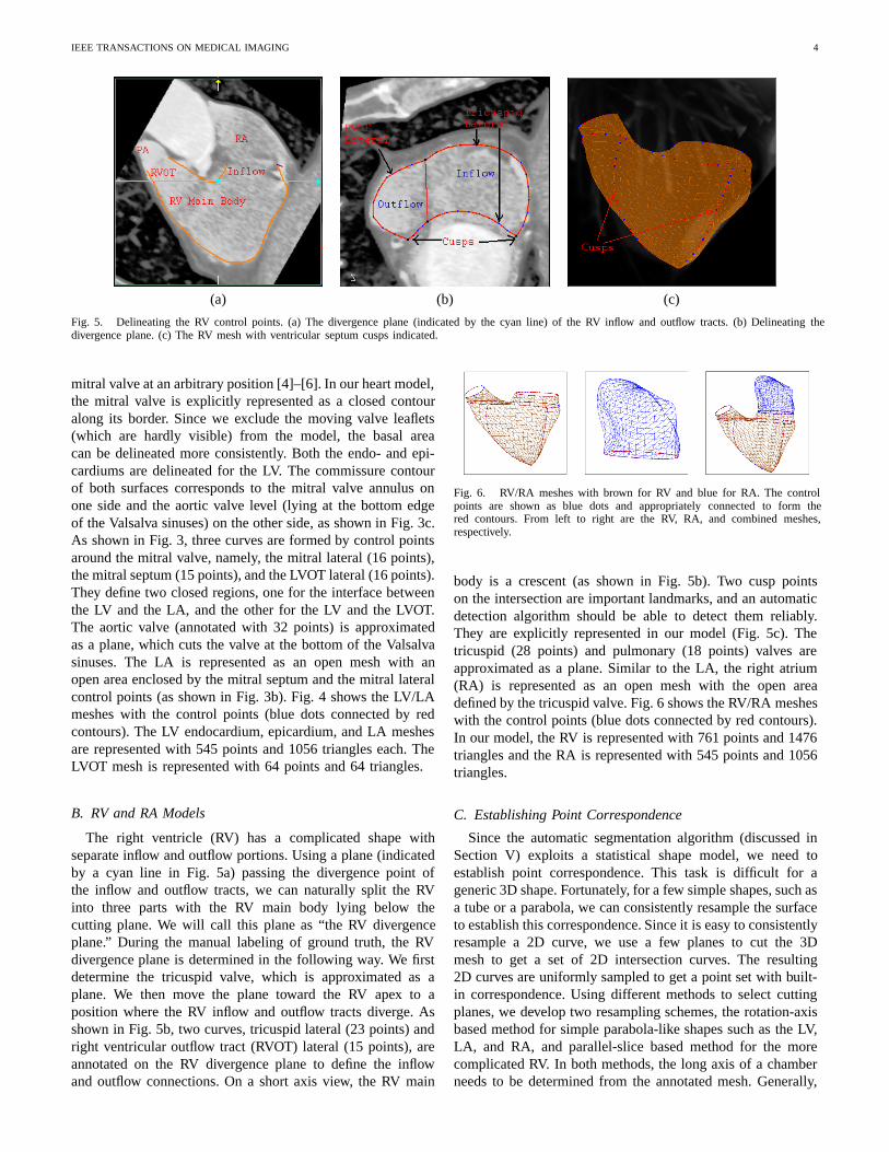
Fig. 5. Delineating the RV control points. (a) The divergence plane (indicated by the cyan line) of the RV inflow and outflow tracts. (b) Delineating thedivergence plane. (c) The RV mesh with ventricular septum cusps indicated.

mitral valve at an arbitrary position [4]–[6]. In our heart model,the mitral valve is explicitly represented as a closed contouralong its border. Since we exclude the moving valve leaflets(which are hardly visible) from the model, the basal areacan be delineated more consistently. Both the endo- and epi-cardiums are delineated for the LV. The commissure contourof both surfaces corresponds to the mitral valve annulus onone side and the aortic valve level (lying at the bottom edgeof the Valsalva sinuses) on the other side, as shown in Fig. 3c.As shown in Fig. 3, three curves are formed by control pointsaround the mitral valve, namely, the mitral lateral (16 points),the mitral septum (15 points), and the LVOT lateral (16 points).They define two closed regions, one for the interface betweenthe LV and the LA, and the other for the LV and the LVOT.The aortic valve (annotated with 32 points) is approximatedas a plane, which cuts the valve at the bottom of the Valsalvasinuses. The LA is represented as an open mesh with anopen area enclosed by the mitral septum and the mitral lateralcontrol points (as shown in Fig. 3b). Fig. 4 shows the LV/LAmeshes with the control points (blue dots connected by redcontours). The LV endocardium, epicardium, and LA meshesare represented with 545 points and 1056 triangles each. TheLVOT mesh is represented with 64 points and 64 triangles.

B. RV and RA Models

The right ventricle (RV) has a complicated shape withseparate inflow and outflow portions. Using a plane (indicatedby a cyan line in Fig. 5a) passing the divergence point ofthe inflow and outflow tracts, we can naturally split the RVinto three parts with the RV main body lying below thecutting plane. We will call this plane as “the RV divergenceplane.” During the manual labeling of ground truth, the RVdivergence plane is determined in the following way. We firstdetermine the tricuspid valve, which is approximated as aplane. We then move the plane toward the RV apex to aposition where the RV inflow and outflow tracts diverge. Asshown in Fig. 5b, two curves, tricuspid lateral (23 points) andright ventricular outflow tract (RVOT) lateral (15 points), areannotated on the RV divergence plane to define the inflowand outflow connections. On a short axis view, the RV main

Fig. 6. RV/RA meshes with brown for RV and blue for RA. The controlpoints are shown as blue dots and appropriately connected to form thered contours. From left to right are the RV, RA, and combined meshes,respectively.

body is a crescent (as shown in Fig. 5b). Two cusp pointson the intersection are important landmarks, and an automaticdetection algorithm should be able to detect them reliably.They are explicitly represented in our model (Fig. 5c). Thetricuspid (28 points) and pulmonary (18 points) valves areapproximated as a plane. Similar to the LA, the right atrium(RA) is represented as an open mesh with the open areadefined by the tricuspid valve. Fig. 6 shows the RV/RA mesheswith the control points (blue dots connected by red contours).In our model, the RV is represented with 761 points and 1476triangles and the RA is represented with 545 points and 1056triangles.

C. Establishing Point Correspondence

Since the automatic segmentation algorithm (discussed inSection V) exploits a statistical shape model, we need toestablish point correspondence. This task is difficult for ageneric 3D shape. Fortunately, for a few simple shapes, such asa tube or a parabola, we can consistently resample the surfaceto establish this correspondence. Since it is easy to consistentlyresample a 2D curve, we use a few planes to cut the 3Dmesh to get a set of 2D intersection curves. The resulting2D curves are uniformly sampled to get a point set with built-in correspondence. Using different methods to select cuttingplanes, we develop two resampling schemes, the rotation-axisbased method for simple parabola-like shapes such as the LV,LA, and RA, and parallel-slice based method for the morecomplicated RV. In both methods, the long axis of a chamberneeds to be determined from the annotated mesh. Generally,


(a) (b) (c)

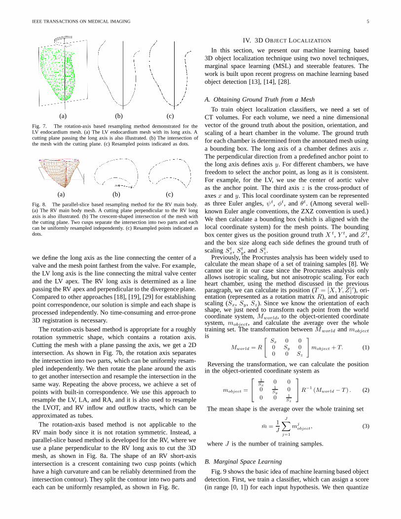
Fig. 7. The rotation-axis based resampling method demonstrated for theLV endocardium mesh. (a) The LV endocardium mesh with its long axis. Acutting plane passing the long axis is also illustrated. (b) The intersection ofthe mesh with the cutting plane. (c) Resampled points indicated as dots.

(a) (b) (c)

Fig. 8. The parallel-slice based resampling method for the RV main body.(a) The RV main body mesh. A cutting plane perpendicular to the RV longaxis is also illustrated. (b) The crescent-shaped intersection of the mesh withthe cutting plane. Two cusps separate the intersection into two parts and eachcan be uniformly resampled independently. (c) Resampled points indicated asdots.

we define the long axis as the line connecting the center of avalve and the mesh point farthest from the valve. For example,the LV long axis is the line connecting the mitral valve centerand the LV apex. The RV long axis is determined as a linepassing the RV apex and perpendicular to the divergence plane.Compared to other approaches [18], [19], [29] for establishingpoint correspondence, our solution is simple and each shape isprocessed independently. No time-consuming and error-prone3D registration is necessary.

The rotation-axis based method is appropriate for a roughlyrotation symmetric shape, which contains a rotation axis.Cutting the mesh with a plane passing the axis, we get a 2Dintersection. As shown in Fig. 7b, the rotation axis separatesthe intersection into two parts, which can be uniformly resam-pled independently. We then rotate the plane around the axisto get another intersection and resample the intersection in thesame way. Repeating the above process, we achieve a set ofpoints with built-in correspondence. We use this approach toresample the LV, LA, and RA, and it is also used to resamplethe LVOT, and RV inflow and outflow tracts, which can beapproximated as tubes.

The rotation-axis based method is not applicable to theRV main body since it is not rotation symmetric. Instead, aparallel-slice based method is developed for the RV, where weuse a plane perpendicular to the RV long axis to cut the 3Dmesh, as shown in Fig. 8a. The shape of an RV short-axisintersection is a crescent containing two cusp points (whichhave a high curvature and can be reliably determined from theintersection contour). They split the contour into two parts andeach can be uniformly resampled, as shown in Fig. 8c.

IV. 3D OBJECT LOCALIZATION

In this section, we present our machine learning based3D object localization technique using two novel techniques,marginal space learning (MSL) and steerable features. Thework is built upon recent progress on machine learning basedobject detection [13], [14], [28].

A. Obtaining Ground Truth from a Mesh

To train object localization classifiers, we need a set ofCT volumes. For each volume, we need a nine dimensionalvector of the ground truth about the position, orientation, andscaling of a heart chamber in the volume. The ground truthfor each chamber is determined from the annotated mesh usinga bounding box. The long axis of a chamber defines axis x.The perpendicular direction from a predefined anchor point tothe long axis defines axis y. For different chambers, we havefreedom to select the anchor point, as long as it is consistent.For example, for the LV, we use the center of aortic valveas the anchor point. The third axis z is the cross-product ofaxes x and y. This local coordinate system can be representedas three Euler angles, ψt, φt, and θt. (Among several well-known Euler angle conventions, the ZXZ convention is used.)We then calculate a bounding box (which is aligned with thelocal coordinate system) for the mesh points. The boundingbox center gives us the position ground truth X t, Y t, and Z t,and the box size along each side defines the ground truth ofscaling St

x, Sty, and St

z .Previously, the Procrustes analysis has been widely used to

calculate the mean shape of a set of training samples [8]. Wecannot use it in our case since the Procrustes analysis onlyallows isotropic scaling, but not anisotropic scaling. For eachheart chamber, using the method discussed in the previousparagraph, we can calculate its position (T = [X,Y, Z] ′), ori-entation (represented as a rotation matrix R), and anisotropicscaling (Sx, Sy , Sz). Since we know the orientation of eachshape, we just need to transform each point from the worldcoordinate system, Mworld, to the object-oriented coordinatesystem, mobject, and calculate the average over the wholetraining set. The transformation between Mworld and mobjectis

Mworld = R

[Sx 0 00 Sy 00 0 Sz

]mobject + T. (1)

Reversing the transformation, we can calculate the positionin the object-oriented coordinate system as

mobject =

⎡⎣ 1

Sx0 0

0 1Sy

0

0 0 1Sz

⎤⎦R−1 (Mworld − T ) . (2)

The mean shape is the average over the whole training set

m =1

J

J∑j=1

mjobject, (3)

where J is the number of training samples.

B. Marginal Space Learning

Fig. 9 shows the basic idea of machine learning based objectdetection. First, we train a classifier, which can assign a score(in range [0, 1]) for each input hypothesis. We then quantize


(a) (b) (c)

Fig. 9. The basic idea of a machine learning based 3D object detection method. (a) A trained classifier that assigns a score to a hypothesis. (b) The parameterspace is quantized into a large number of discrete hypotheses and the classifier is used to select the best hypotheses in exhaustive search. (c) A few hypothesesof the left ventricle (represented as boxes) embedded in a CT volume. The red box shows the ground truth and the green boxes show only a few hypotheses.

Fig. 10. Marginal space learning. A classifier trained on a marginaldistribution p(y) can quickly eliminate a large portion (regions 1 and 3) of thesearch space. Another classifier is then trained on a restricted space (region2) for the joint distribution p(x, y).

the full parameter space into a large number of hypotheses.Each hypothesis is tested with the classifier to get a score.Based on the classification scores, we select the best oneor several hypotheses. Unlike the gradient based search indeformable models or active appearance models (AAM) [30],the classifier in this framework acts as a black box without anexplicit closed-form objective function.

One drawback of the learning based approach is that thenumber of hypotheses increases exponentially with respect tothe dimension of the parameter space. We observed that, inmany real applications, the posterior distribution is clusteredin a small region in the high dimensional parameter space.Therefore, the uniform and exhaustive search is not necessaryand wastes the computational power. Fig. 10 illustrates asimple example for 2D space search. A classifier trainedon p(y) can quickly eliminate a large portion of the searchspace. We can then train a classifier in a much smaller region(region 2 in Fig. 10) for joint distribution p(x, y). Basedon this observation, we propose a novel efficient parametersearch method, marginal space learning (MSL), to search suchclustered spaces. In MSL, the dimensionality of the searchspace is gradually increased. As shown in the top dashed boxin Fig. 2, we split 3D object localization into three steps:position estimation, position-orientation estimation, and fullsimilarity transformation estimation. After each step we keepa limited number of candidates to reduce the search space. Toincrease the speed further, we use a pyramid-based coarse-to-fine strategy such that object localization is performed on alow-resolution (3 mm) volume.

To train a classifier, we need to split a set of hypothesesinto two groups, positive and negative, based on their distanceto the ground truth. The error in object position and scaleestimation is not comparable with that of orientation estima-tion. Therefore, a normalized distance measure is defined bynormalizing the error in each dimension to the correspondingsearch step size,

E = maxi=1,...,D

|P ei − P t

i |/SearchStepi, (4)

where P ei is the estimated value for parameter i, P t

i iscorresponding the ground truth, and D is the dimension ofthe parameter space. For similarity transformation estimation,the parameter space is nine dimensional, D = 9. A sample isregarded as a positive one if E ≤ 1.0 and all the others arenegative samples.

C. Training of Position Estimator

In this step, we want to estimate the position of the objectand learning is constrained in a marginal space with threedimensions. Given a hypothesis (X,Y, Z), the classificationproblem is formulated as whether there is an object centeredat (X,Y, Z). Haar wavelet features are fast to compute andhave been shown to be effective for many applications [13],[27]. Therefore, we use 3D Haar wavelet features for learningin this step. Readers are referred to [13], [27] for more details,and [28] for a description of 3D Haar wavelet features.

The search step for position estimation is one voxel. Ac-cording to Eq. (4), a positive sample (X,Y, Z) should satisfy

max{|X −Xt|, |Y − Y t|, |Z − Zt|} ≤ 1 voxel, (5)

where (X t, Y t, Zt) is the ground truth of the object center.Given a set of positive and negative training samples, weextract 3D Haar wavelet features and train a classifier using theprobabilistic boosting-tree (PBT) [31]. After that, we test eachvoxel in a volume one by one as a hypothesis of the objectposition using the trained classifier. As shown in Fig. 9a, theclassifier assigns each hypothesis a score, and we preserve asmall number of candidates (100 in our experiments) with thehighest detection score for each volume.

D. Steerable Features

Before discussing our technique for the position-orientationand full similarity transformation estimation, we present an-other major contribution of this paper, steerable features.


(a) (b) (c)

Fig. 11. Using a regular sampling pattern to incorporate a hypothesis(X, Y, ψ, Sx, Sy) about a 2D object pose. The sampling points are indicatedas ’+’. (a) Move the pattern center to (X, Y ). (b) Align the pattern to theorientation ψ. (c) The final aligned sampling pattern after scaling along eachaxis, proportional to (Sx, Sy).

Global features, such as 3D Haar wavelet features, are effectiveto capture the global information (e.g., orientation and scale)of an object. To capture the orientation information of ahypothesis, we should rotate either the volume or the featuretemplates. However, it is time consuming to rotate a 3Dvolume and there is no efficient way to rotate the Haar waveletfeature templates. Local features are fast to evaluate but losethe global information of the whole object.

In this paper, we propose a new framework, steerablefeatures, which can capture the orientation and scale of theobject and at the same time be very efficient. In steerablefeatures, we sample a few points from the volume under asampling pattern. We then extract a few local features foreach sampling point (e.g., voxel intensity and gradient) fromthe original volume. The novelty of our steerable featuresis that we embed the orientation and scale information intothe distribution of sampling points, while each individualfeature is locally defined. Instead of aligning the volume tothe hypothesized orientation, we steer the sampling pattern.This is where the name “steerable features” comes from.

Fig. 11 shows how to embed a hypothesis in steerablefeatures using a regular sampling pattern (illustrated for a 2Dcase for clearance in visualization). Suppose we want to test ifhypothesis (X,Y, Z, ψ, φ, θ, Sx, Sy, Sz) is a good estimationof the similarity transformation of the object. A local coordi-nate system is defined to be centered at position (X,Y, Z)(Fig. 11a) and the axes are aligned with the hypothesizedorientation (ψ, φ, θ) (Fig. 11b). A few points (represented as‘+’ in Fig. 11) are uniformly sampled along each coordinateaxis inside a box. The sampling distance along an axis isproportional to the scale of the shape in that direction (Sx,Sy , or Sz) to incorporate the scale information (Fig. 11c). Thesteerable features constitute a general framework, in whichdifferent sampling patterns [15], [32] can be defined.

At each sampling point, we extract a few local featuresbased on the intensity and gradient from the original volume.A major reason to select these features is that they can beextracted fast. Suppose a sampling point (x, y, z) has intensityI and gradient g = (gx, gy, gz). The three axes of object-oriented local coordinate system are nx, ny, and nz . The anglebetween the gradient g and the z axis is α = arccos(nz .g),where nz.g means the inner product between two vectors nz

and g. The following 24 features are extracted: I ,√I , 3

√I ,

I2, I3, log I , ‖g‖,√‖g‖, 3

√‖g‖, ‖g‖2, ‖g‖3, log ‖g‖, α,√α,

3√α, α2, α3, logα, gx, gy, gz , nx.g, ny.g, nz.g. In total, we

have 24 local features for each sampling point. The first sixfeatures are based on intensity and the remaining 18 featuresare transformations of gradients. Feature transformation, atechnique often used in pattern classification, is a processthrough which a new set of features is created [33]. We use itto enhance the feature set by adding a few transformations ofan individual feature. Suppose there are P sampling points, weget a feature pool containing 24×P features. (In our case, the5×5×5 regular sampling pattern is used for object localization,resulting in P = 125 sampling points.) These features areused to train histogram-based weak classifiers [34] and weuse the probabilistic boosting-tree (PBT) [31] to combine themto get a strong classifier. Following are some statistics aboutthe selected features by the boosting algorithm. Combiningfeatures in all object localization classifiers, overall, thereare 3696 features selected. We found each feature type wasselected as least once. The intensity features, I ,

√I , 3

√I , I2,

I3, log I , counted about 26% of the selected features, while,the following four gradient-based features, gx, gy, gz , and ‖g‖,counted about 34%.

E. Training of Position-Orientation Estimator

In this step, we want to jointly estimate the position and ori-entation. The classification problem is formulated as whetherthere is an object centered at (X,Y, Z) with orientation(ψ, φ, θ). After object position estimation, we preserve the top100 candidates, (Xi, Yi, Zi), i = 1, . . . , 100. Since we want toestimate both the position and orientation, we need to augmentthe dimension of candidates. For each position candidate, wequantize the orientation space uniformly to generate hypothe-ses. The orientation is represented as three Euler angles inthe ZXZ convention, ψ, φ, and θ. The distribution range ofan Euler angle be estimated from the training data. EachEuler angle is quantized within the range using a step size of0.2 radians (11 degrees). For each candidate (X i, Yi, Zi), weaugment it with N (about 1000) hypotheses about orientation,(Xi, Yi, Zi, ψj , φj , θj), j = 1, . . . , N . Some are close to theground truth (positive) and others are far away (negative). Thelearning goal is to distinguish the positive and negative sam-ples using trained classifiers. Using the normalized distancemeasure of Eq. (4), a hypothesis (X,Y, Z, ψ, φ, θ) is regardedas a positive sample if it satisfies both Eq. (5) and

max{|ψ − ψt|, |φ− φt|, |θ − θt|} ≤ 0.2, (6)

where (ψt, φt, θt) represent the orientation ground truth. Allthe other hypotheses are regarded as negative samples. Torepresent the orientation information, we have to rotate eitherthe volume or feature templates. We use the steerable features,which are efficient under rotation. Similarly, the PBT is usedfor training and the trained classifier is used to prune thehypotheses to preserve only a few candidates (50 in ourexperiments).

F. Training of Similarity Transformation Estimator

The similarity transformation (adding the scales) estimationstep is analogous to position-orientation estimation exceptlearning is performed in the full nine dimensional similarity


(a) (b) (c)

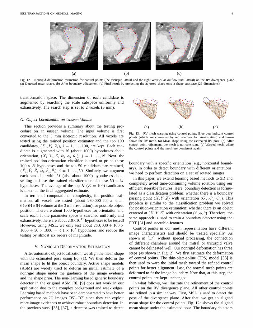
Fig. 12. Nonrigid deformation estimation for control points (the tricuspid lateral and the right ventricular outflow tract lateral) on the RV divergence plane.(a) Detected mean shape. (b) After boundary adjustment. (c) Final result by projecting the adjusted shape onto a shape subspace (25 dimensions).

transformation space. The dimension of each candidate isaugmented by searching the scale subspace uniformly andexhaustively. The search step is set to 2 voxels (6 mm).

G. Object Localization on Unseen Volume

This section provides a summary about the testing pro-cedure on an unseen volume. The input volume is firstconverted to the 3 mm isotropic resolution. All voxels aretested using the trained position estimator and the top 100candidates, (Xi, Yi, Zi), i = 1, . . . , 100, are kept. Each can-didate is augmented with N (about 1000) hypotheses aboutorientation, (Xi, Yi, Zi, ψj , φj , θj), j = 1, . . . , N . Next, thetrained position-orientation classifier is used to prune these100 × N hypotheses and the top 50 candidates are retained,(Xi, Yi, Zi, ψi, φi, θi), i = 1, . . . , 50. Similarly, we augmenteach candidate with M (also about 1000) hypotheses aboutscaling and use the trained classifier to rank these 50 × Mhypotheses. The average of the top K (K = 100) candidatesis taken as the final aggregated estimate.

In terms of computational complexity, for position esti-mation, all voxels are tested (about 260,000 for a small64×64×64 volume at the 3 mm resolution) for possible objectposition. There are about 1000 hypotheses for orientation andscale each. If the parameter space is searched uniformly andexhaustively, there are about 2.6×1011 hypotheses to be tested!However, using MSL, we only test about 260, 000 + 100 ×1000 + 50 × 1000 = 4.1 × 105 hypotheses and reduce thetesting by almost six orders of magnitude.

V. NONRIGID DEFORMATION ESTIMATION

After automatic object localization, we align the mean shapewith the estimated pose using Eq. (1). We then deform themean shape to fit the object boundary. Active shape models(ASM) are widely used to deform an initial estimate of anonrigid shape under the guidance of the image evidenceand the shape prior. The non-learning based generic boundarydetector in the original ASM [8], [9] does not work in ourapplication due to the complex background and weak edges.Learning based methods have been demonstrated to have betterperformance on 2D images [35]–[37] since they can exploitmore image evidences to achieve robust boundary detection. Inthe previous work [35], [37], a detector was trained to detect

(a) (b) (c)

Fig. 13. RV mesh warping using control points. Blue dots indicate controlpoints (which are connected by red contours for visualization) and brownshows the RV mesh. (a) Mean shape using the estimated RV pose. (b) Aftercontrol point refinement, the mesh is not consistent. (c) Warped mesh, wherethe control points and the mesh are consistent again.

boundary with a specific orientation (e.g., horizontal bound-ary). In order to detect boundary with different orientations,we need to perform detection on a set of rotated images.

In this paper, we extend learning based methods to 3D andcompletely avoid time-consuming volume rotation using ourefficient steerable features. Here, boundary detection is formu-lated as a classification problem: whether there is a boundarypassing point (X,Y, Z) with orientation (Ox, Oy , Oz). Thisproblem is similar to the classification problem we solvedfor position-orientation estimation: whether there is an objectcentered at (X,Y, Z) with orientation (ψ, φ, θ). Therefore, thesame approach is used to train a boundary detector using thePBT [31] and steerable features.

Control points in our mesh representation have differentimage characteristics and should be treated specially. Asshown in [17], without special processing, the connectionof different chambers around the mitral or tricuspid valvecannot be delineated well. Our nonrigid deformation has threesteps (as shown in Fig. 2). We first estimate the deformationof control points. The thin-plate-spline (TPS) model [38] isthen used to warp the initial mesh toward the refined controlpoints for better alignment. Last, the normal mesh points aredeformed to fit the image boundary. Note that, at this step, thecontrol points are kept unchanged.

In what follows, we illustrate the refinement of the controlpoints on the RV divergence plane. All other control pointsare refined in a similar way. First, MSL is used to detect thepose of the divergence plane. After that, we get an alignedmean shape for the control points. Fig. 12a shows the alignedmean shape under the estimated pose. The boundary detectors


(a) (b) (c)

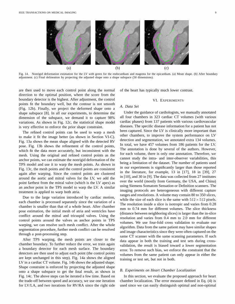
Fig. 14. Nonrigid deformation estimation for the LV with green for the endocardium and magenta for the epicardium. (a) Mean shape. (b) After boundaryadjustment. (c) Final delineation by projecting the adjusted shape onto a shape subspace (50 dimensions).

are then used to move each control point along the normaldirection to the optimal position, where the score from theboundary detector is the highest. After adjustment, the controlpoints fit the boundary well, but the contour is not smooth(Fig. 12b). Finally, we project the deformed shape onto ashape subspace [8]. In all our experiments, to determine thedimension of the subspace, we demand it to capture 98%variations. As shown in Fig. 12c, the statistical shape modelis very effective to enforce the prior shape constraint.

The refined control points can be used to warp a meshto make it fit the image better (as shown in Section VI-C).Fig. 13a shows the mean shape aligned with the detected RVpose. Fig. 13b shows the refinement of the control points,which fit the data more accurately, but inconsistent with themesh. Using the original and refined control points as theanchor points, we can estimate the nonrigid deformation of theTPS model and use it to warp the mesh points. As shown inFig. 13c, the mesh points and the control points are consistentagain after warping. Since the control points are clusteredaround the aortic and mitral valves for the LV, we add thepoint farthest from the mitral valve (which is the LV apex) asan anchor point in the TPS model to warp the LV. A similartreatment is applied to warp both atria.

Due to the large variation introduced by cardiac motion,each chamber is processed separately since the variation of achamber is smaller than that of a whole heart. After chamberpose estimation, the initial mesh of atria and ventricles haveconflict around the mitral and tricuspid valves. Using thecontrol points around the valves as anchor points in TPSwarping, we can resolve such mesh conflict. After the wholesegmentation procedure, further mesh conflict can be resolvedthrough a post-processing step.

After TPS warping, the mesh points are closer to thechamber boundary. To further reduce the error, we train againa boundary detector for each mesh surface. The boundarydetectors are then used to adjust each point (the control pointsare kept unchanged in this step). Fig. 14a shows the alignedLV in a cardiac CT volume. Fig. 14b shows the adjusted shape.Shape constraint is enforced by projecting the adjusted shapeonto a shape subspace to get the final result, as shown inFig. 14c. The above steps can be iterated a few time. Based onthe trade-off between speed and accuracy, we use one iterationfor LV/LA, and two iterations for RV/RA since the right side

of the heart has typically much lower contrast.

VI. EXPERIMENTS

A. Data Set

Under the guidance of cardiologists, we manually annotatedall four chambers in 323 cardiac CT volumes (with variouscardiac phases) from 137 patients with various cardiovasculardiseases. The specific disease information for a patient has notbeen captured. Since the LV is clinically more important thanother chambers, to improve the system performance on LVdetection and segmentation, we annotated extra 134 volumes.In total, we have 457 volumes from 186 patients for the LV.The annotation is done by several of the authors. However,for each volume, there is only one annotation. Therefore, wecannot study the intra- and inter-observer variabilities, thisbeing a limitation of the dataset. The number of patients usedin our experiments is significantly larger than those reportedin the literature, for example, 13 in [17], 18 in [39], 27in [10], and 30 in [9]. The data was collected from 27 institutesover the world (mostly from Germany, the USA, and China)using Siemens Somatom Sensation or Definition scanners. Theimaging protocols are heterogeneous with different captureranges and resolutions. A volume may contain 80 to 350 slices,while the size of each slice is the same with 512×512 pixels.The resolution inside a slice is isotropic and varies from 0.28mm to 0.74 mm for different volumes. The slice thickness(distance between neighboring slices) is larger than the in-sliceresolution and varies from 0.4 mm to 2.0 mm for differentvolumes. We use four-fold cross validation to evaluate ouralgorithm. Data from the same patient may have similar shapesand image characteristics since they were often captured on thesame CT scanner with the same scanning parameters. If suchdata appear in both the training and test sets during cross-validation, the result is biased toward a lower segmentationerror. To remove such bias, we enforce the constraint that thevolumes from the same patient can only appear in either thetraining or test set, but not in both.

B. Experiments on Heart Chamber Localization

In this section, we evaluate the proposed approach for heartchamber localization. The error measure defined in Eq. (4) isused since we can easily distinguish optimal and non-optimal


0 50 100 150 200 250 300 350 4000

0.5

1

1.5

2

2.5

3

3.5Position Estimation

Number of Candidates

Min

imum

Err

or

LVLARVRALower Bound

0 50 100 150 200 250 300 350 4000

0.25

0.5

0.75

1

1.25

1.5

1.75

2Position−Orientation Estimation


Min

imum

Err

or

LVLARVRALower Bound

0 50 100 150 200 250 300 350 4000

0.5

1

1.5

2

2.5Position−Orientation−Scale Estimation


Min

imum

Err

or

LVLARVRALower Bound

(a) (b) (c)

Fig. 15. The error, defined in Eq. (4), of the best candidate with respect to the number of candidates preserved after each step. (a) Position estimation. (b)Position-orientation estimation. (c) Full similarity transformation estimation. The red dotted lines show the lower bound of the detection error.

estimates, compared to other error measures (e.g., the weightedEuclidean distance). The optimal estimate is up-bounded by0.5 search steps under any search grid. However, a non-optimalestimate has an error larger than 0.5.

The efficiency of MSL comes from the fact that we prunethe search space after each step. One concern is that sincethe space is not fully explored, it may miss the optimalsolution at an early stage. In the following, we demonstratethat accuracy only deteriorates slightly in MSL. Fig. 15 showsthe error of the best candidate after each step with respect tothe number of candidates preserved. The curves are calculatedon all volumes based on cross validation. The red dotted linesshow the error of the optimal solution under the search grid.As shown in Fig. 15a for position estimation, if we keeponly one candidate, the average error may be as large as 3.5voxels. However, by retaining more candidates, the minimumerrors decrease quickly. We have a high probability to keepthe optimal solution when 100 candidates are preserved. Weobserved the same trend in different marginal spaces, such asthe position-orientation space as shown in Fig. 15b. Basedon the trade-off between accuracy and speed, we preserve50 candidates after position-orientation estimation. After fullsimilarity transformation estimation, the best candidates we gethave an error ranging from 1.0 to 1.4 search steps as shown inFig. 15c. Using the average of the topK (K = 100) candidatesas the final single estimate, we achieve an error of about 1.5 to2.0 search steps for different chambers. Our approach is robustand we did not observe any major failure. For comparison, theheart localization modules in both [17] and [9] failed on about10% volumes.

C. Experiments on Boundary Delineation

In this section, we evaluate our approach for boundary delin-eation. As a widely used criterion [9], [10], [17], the symmetricpoint-to-mesh distance, Ep2m, is exploited to measure theaccuracy in surface boundary delineation. For each point ona mesh, we search for the closest point (not necessarily meshtriangle vertices) on the other mesh to calculate the minimumEuclidean distance. We calculate the point-to-mesh distancefrom the detected mesh to the ground-truth and vice versa tomake the measurement symmetric.

In our experiments, we estimate the pose of each chamberseparately. Therefore, we use 4 × 9 = 36 pose parameters to

align the mean shapes. As shown in the second column ofTable I, the mean Ep2m error after heart localization is 3.17mm for the LV endocardium, 2.51 mm for the LV epicardium,2.78 mm for the LA, 2.93 mm for the RV, and 3.09 mm for theRA. Alternatively, we can treat the whole heart as one objectin heart localization, then we use only nine pose parameters.In this way, the mean Ep2m error achieved is 3.52 mm forthe LV endocardium, 3.07 mm for the LV epicardium, 3.95mm for LA, 3.94 mm for the RV, and 4.64 mm for the RA.Obviously, treating each chamber separately, we can obtain abetter initialization.

In our nonrigid deformation estimation, control points andnormal mesh points are treated differently. We first estimatethe deformation of control points and use TPS warping tomake the mesh consistent after warping. As shown in thethird column in Table I, after control point based alignment,we slightly reduce the error for the LV, LA, and RA by 5%and significantly reduce the error by 17% for the RV sincethe control points are more uniformly distributed in the RVmesh. After deformation estimation of all mesh points, thefinal segmentation error ranges from 1.13 mm to 1.57 mm fordifferent chambers. The LV and LA have smaller errors thanthe RV and RA due to the use of contrast agent in the leftheart (as shown in Fig. 16).

We compare our approach to the baseline ASM using non-learning based boundary detection scheme [8]. The com-parison is limited to the last step on normal mesh pointdeformation. Input for both algorithms are the same initializedmesh. The iteration number in the baseline ASM is tuned togive the best performance. As shown in Table I, the baselineASM actually increase the error for weak boundaries (e.g.,the LV epicardium and RV). It performs well for strongboundaries, such as the LV endocardium and the LA, but it isstill significantly worse than the proposed method.

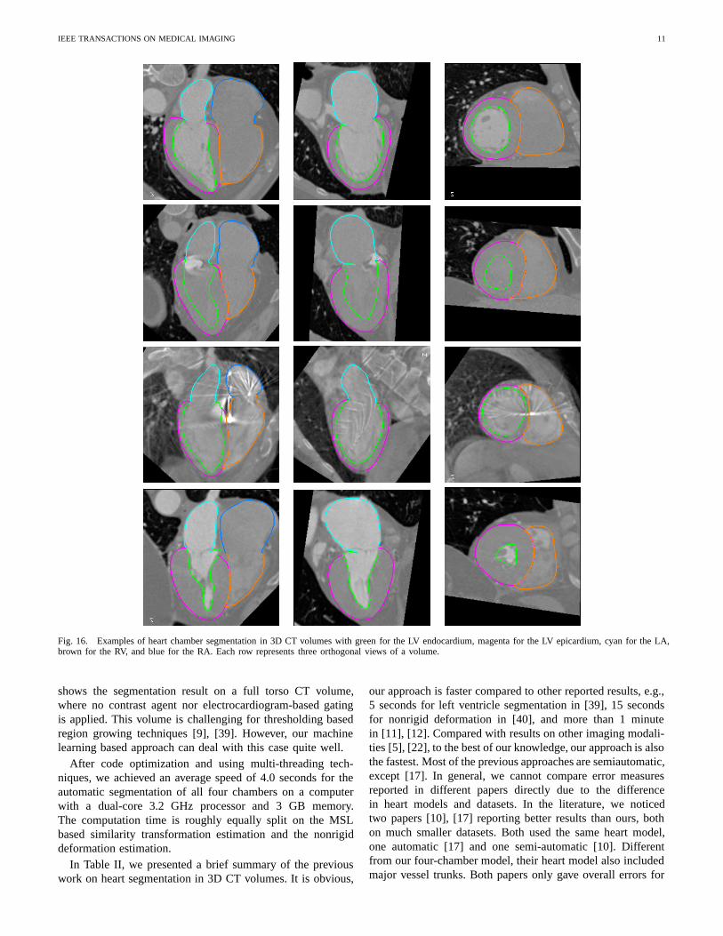
Fig. 16 shows several examples for heart chamber seg-mentation using the proposed approach. It performs well onvolumes with low contrast (as shown in the second row ofFig. 16) and it is robust even under severe streak artifacts(as shown in the third example). Since our system is trainedon volumes from all phases from a cardiac cycle, we canprocess volumes from the end-systolic phase (which hasa significantly small blood pool for the LV) without anydifficulty, as shown in the last example in Fig. 16. Fig. 17


Fig. 16. Examples of heart chamber segmentation in 3D CT volumes with green for the LV endocardium, magenta for the LV epicardium, cyan for the LA,brown for the RV, and blue for the RA. Each row represents three orthogonal views of a volume.

shows the segmentation result on a full torso CT volume,where no contrast agent nor electrocardiogram-based gatingis applied. This volume is challenging for thresholding basedregion growing techniques [9], [39]. However, our machinelearning based approach can deal with this case quite well.

After code optimization and using multi-threading tech-niques, we achieved an average speed of 4.0 seconds for theautomatic segmentation of all four chambers on a computerwith a dual-core 3.2 GHz processor and 3 GB memory.The computation time is roughly equally split on the MSLbased similarity transformation estimation and the nonrigiddeformation estimation.

In Table II, we presented a brief summary of the previouswork on heart segmentation in 3D CT volumes. It is obvious,

our approach is faster compared to other reported results, e.g.,5 seconds for left ventricle segmentation in [39], 15 secondsfor nonrigid deformation in [40], and more than 1 minutein [11], [12]. Compared with results on other imaging modali-ties [5], [22], to the best of our knowledge, our approach is alsothe fastest. Most of the previous approaches are semiautomatic,except [17]. In general, we cannot compare error measuresreported in different papers directly due to the differencein heart models and datasets. In the literature, we noticedtwo papers [10], [17] reporting better results than ours, bothon much smaller datasets. Both used the same heart model,one automatic [17] and one semi-automatic [10]. Differentfrom our four-chamber model, their heart model also includedmajor vessel trunks. Both papers only gave overall errors for


TABLE I

MEAN AND STANDARD DEVIATION (IN PARENTHESES) OF THE POINT-TO-MESH ERROR (IN MILLIMETERS) FOR THE SEGMENTATION OF HEART

CHAMBERS BASED ON CROSS VALIDATION.

After RigidLocalization

After Control PointDeformation and Warping Baseline ASM [8] Proposed Approach

Left Ventricle Endocardium 3.17 (1.10) 3.00 (1.11) 2.24 (1.21) 1.13 (0.55)Left Ventricle Epicardium 2.51 (0.78) 2.35 (0.73) 2.45 (1.02) 1.21 (0.41)

Left Atrium 2.78 (0.98) 2.67 (1.01) 1.89 (1.43) 1.32 (0.42)Right Ventricle 2.93 (0.75) 2.40 (0.82) 2.69 (1.10) 1.55 (0.38)Right Atrium 3.09 (0.86) 2.90 (0.92) 2.81 (1.15) 1.57 (0.48)

TABLE II

COMPARISON WITH PREVIOUS WORK ON HEART SEGMENTATION IN 3D CT VOLUMES.

Patients/Subjects Volumes Chambers Automatic Speed

Point-to-MeshError (mm)

Neubauer and Wegenkiltl [11] N/A N/A Left ventricle No >1 min N/AMcInerney and Terzopoulos [12] 1 16 Left ventricle No 100 mina N/A

Fritz et al. [9] 30 30 Left ventricle No N/A 1.5Jolly [39] 18 36 Left ventricle Nob ∼5 s N/A

Ecabert et al. [17] 13 28 Four chambers and vessel trunks Yesc N/A 0.85d

Lorenz and von Berg [10] 27 27 Four chambers and vessel trunks No N/A 0.81-1.19von Berg and Lorenz [40] 6 60 Four chambers and vessel trunks No 15 s N/A

Our approach 137+ 323+ Four chambers Yes 4.0 s 1.13-1.57a This was the time used to process the whole sequence of 16 volumes.b The long axis of the left ventricle needed to be manually aligned. All other steps were automatic.c The success rate of automatic heart localization was about 90%.d Gross failures in heart localization were excluded from evaluation.

Fig. 17. Heart chamber segmentation result for a low-contrast full-torso CT volume. The first column shows a full torso view and the right three columnsshow close-up views.

the whole heart model (including the major vessel trunks),without any break-down error measure for each chamber.Some care needs to be taken to compare our approach withthese two papers. 1) Ecabert et al. [17] admitted that it washard to distinguish the boundary of different chambers. Forexample, it was likely to include a part of the LA in thesegmented LV mesh and vice verse. Such errors were onlypartially penalized in both [17] and [10] since they did notprovide break-down error measure for each chamber. However,in our evaluation, we fully penalize such errors. 2) About8% mesh points around the connection of vessel trunks toheart chambers were excluded for evaluation in [17]. In theirmodel, all chambers and vessel trunks were artificially closed.Since there are no image features around these artificial caps,these regions cannot be delineated accurately even by anexpert. Based on this consideration, they were removed fromevaluation. In our model, all valves are represented as closedcontours along their borders in our heart model. We only needto delineate the border of the valves and this can be donemore accurately. Therefore, no mesh part is excluded from

evaluation. 3) In [17], the automatic heart localization modulefailed on about 10% volumes and such gross failures werealso excluded for evaluation. 4) In [10], only volumes fromthe end-diastolic phase were used for experiments. However,our dataset contains 323+ volumes from all cardiac phases.The size and shape of a chamber change significantly fromthe end-diastolic phase to the end-systolic phase. Therefore,there is much more variance in our dataset.

D. Heart Chamber Tracking

The size and shape of a heart chamber (especially, the LV)change significantly from an expansion phase to a contractionphase. Since our system is trained on volumes from all phasesin a cardiac cycle, we can reliably detect and segment the heartfrom any cardiac phase. By performing heart segmentationframe by frame, the heart motion is tracked in the robusttracking-by-detection framework. To make the motion moreconsistent, mild motion smoothing is applied after the segmen-tation of each frame. Fig. 18 shows the tracking results on one


TABLE III

THE EJECTION FRACTION (EF) ESTIMATION ACCURACY FOR ALL SIX DYNAMIC SEQUENCES IN OUR DATASET.

Patient #1 Patient #2 Patient #3 Patient #4 Patient #5 Patient #6 Mean Error Standard DeviationGround Truth 68.7% 49.7% 45.8% 62.9% 47.4% 38.9% 2.3% 1.6%

Estimation 66.8% 51.8% 42.8% 64.4% 42.3% 38.5%

Fig. 18. Tracking results for the heart chambers on a dynamic 3D sequence with 10 frames. Four frames (1, 2, 3, and 6) are shown here.

1 2 3 4 5 6 7 8 9 1030

40

50

60

70

80

90

100

110

Frame

Vol

ume

(ml)

Detection (EF=67%)Ground−truth (EF=69%)

1 2 3 4 5 6 7 8 9 1050

60

70

80

90

100

110

120

130

Frame

Vol

ume

(ml)

Detection (EF=52%)Ground−truth (EF=50%)

Fig. 19. The left ventricle volume-time curves for two dynamic 3Dsequences.

sequence. To further improve the system performance, we canexploit a motion model learned in an annotated dataset [41],but it is out of the scope of this paper.

The motion pattern of a chamber during a cardiac cycleprovides many important clinical measurements of its func-tionality, e.g., the ventricular ejection fraction, myocardiumwall thickness, and dissynchrony within a chamber or betweendifferent chambers [2]. Given the tracking result, we cancalculate the ejection fraction (EF) as follows,

EF =VolumeED − VolumeES

VolumeED, (7)

where VolumeED and VolumeES are the volume measuresof the end-diastolic (ED) and end-systolic (ES) phases, re-spectively. In our dataset, there are six patients each with 10frames from the whole cardiac cycle. Due to the space limit,Fig. 19 shows the LV volume-time curves for two dynamicsequences. Table III shows the EF estimation accuracy for allsix sequences. The estimated EFs are close to the ground truthwith a mean error of 2.3%.

VII. CONCLUSIONS AND FUTURE WORK

In this paper, we proposed a novel four-chamber surfacemesh model for a heart. In heart modeling, the following twofactors are considered and traded-off: 1) accuracy in anatomyand 2) easiness for both annotation and automatic detection. Tomore accurately represent the anatomy, important landmarkssuch as valves and ventricular septum cusps are explicitly

represented in our model. These landmarks can be detectedreliably to guide the automatic model fitting process.

Using this model, we develop an efficient and robust ap-proach for automatic heart chamber segmentation in 3D CTvolumes. The efficiency of our approach comes from thetwo new techniques, marginal space learning and steerablefeatures. We achieved an average speed of 4.0 seconds pervolume to segment all four chambers. Robustness is achievedby using recent advances in learning discriminative modelsand exploiting a large annotated dataset. All major steps inour approach are learning-based, therefore minimizing thenumber of underlying model assumptions. According to ourknowledge, this is the first study reporting stable results ona large cardiac CT dataset. Our segmentation approach isgeneral and we have extensively tested it on many challenging3D detection and segmentation tasks in medical imaging(e.g., ileocecal valves, polyps [42], and livers in abdominalCT [32], brain tissues [43] and heart chambers in ultrasoundimages [41], [44], and heart chambers in MRI).

VIII. ACKNOWLEDGES

The authors would like to thank the anonymous reviewersfor their constructive comments.

REFERENCES

[1] P. Schoenhagen, S.S. Halliburton, A.E. Stillman, and R.D. White, “CT ofthe heart: Principles, advances, clinical uses,” Cleveland Clinic Journalof Medicine, vol. 72, no. 2, pp. 127–138, 2005.

[2] A.F. Frangi, W.J. Niessen, and M.A. Viergever, “Three-dimensionalmodeling for functional analysis of cardiac images: A review,” IEEETrans. Medical Imaging, vol. 20, no. 1, pp. 2–25, 2001.

[3] A.F. Frangi, D. Rueckert, and J.S. Duncan, “Three-dimensional cardio-vascular image analysis,” IEEE Trans. Medical Imaging, vol. 21, no. 9,pp. 1005–1010, 2002.

[4] J. Lotjonen, S. Kivisto, J. Koikkalainen, D. Smutek, and K. Lauerma,“Statistical shape model of atria, ventricles and epicardium from short-and long-axis MR images,” Medical Image Analysis, vol. 8, no. 3, pp.371–386, 2004.

[5] W. Hong, B. Georgescu, X.S. Zhou, S. Krishnan, Y. Ma, and D. Co-maniciu, “Database-guided simultaneous multi-slice 3D segmentationfor volumetric data,” in Proc. European Conf. Computer Vision, 2006,pp. 397–409.


[6] D. Fritz, D. Rinck, R. Dillmann, and M. Scheuring, “Segmentation of theleft and right cardiac ventricle using a combined bi-temporal statisticalmodel,” in Proc. of SPIE Medical Imaging, 2006, pp. 605–614.

[7] R. Ionasec, B. Georgescu, E. Gassner, S. Vogt, O. Kutter, M. Scheuering,N. Navab, and D. Comaniciu, “Dynamic model-driven quantitative andvisual evaluation of the aortic valve from 4D CT,” in Proc. Int’l Conf.Medical Image Computing and Computer Assisted Intervention, 2008.

[8] T.F. Cootes, C.J. Taylor, D.H. Cooper, and J. Graham, “Active shapemodels—their training and application,” Computer Vision and ImageUnderstanding, vol. 61, no. 1, pp. 38–59, 1995.

[9] D. Fritz, D. Rinck, R. Unterhinninghofen, R. Dillmann, and M. Scheur-ing, “Automatic segmentation of the left ventricle and computation ofdiagnostic parameters using regiongrowing and a statistical model,” inProc. of SPIE Medical Imaging, 2005, pp. 1844–1854.

[10] C. Lorenz and J. von Berg, “A comprehensive shape model of the heart,”Medical Image Analysis, vol. 10, no. 4, pp. 657–670, 2006.

[11] A. Neubauer and R. Wegenkiltl, “Analysis of four-dimensional cardiacdata sets using skeleton-based segmentation,” in Proc. Int’l Conf. inCentral Europe on Computer Graphics and Visualization, 2003.

[12] T. McInerney and D. Terzopoulos, “A dynamic finite element surfacemodel for segmentation and tracking in multidimensional medical im-ages with application to cardiac 4D image analysis,” ComputerizedMedical Imaging and Graphics, vol. 19, no. 1, pp. 69–83, 1995.

[13] P. Viola and M. Jones, “Rapid object detection using a boosted cascadeof simple features,” in Proc. IEEE Conf. Computer Vision and PatternRecognition, 2001, pp. 511–518.

[14] B. Georgescu, X.S. Zhou, D. Comaniciu, and A. Gupta, “Database-guided segmentation of anatomical structures with complex appearance,”in Proc. IEEE Conf. Computer Vision and Pattern Recognition, 2005,pp. 429–436.

[15] Y. Zheng, A. Barbu, B. Georgescu, M. Scheuering, and D. Comaniciu,“Fast automatic heart chamber segmentation from 3D CT data usingmarginal space learning and steerable features,” in Proc. Int’l Conf.Computer Vision, 2007.

[16] Y. Zheng, B. Georgescu, A. Barbu, M. Scheuering, and D. Comaniciu,“Four-chamber heart modeling and automatic segmentation for 3Dcardiac CT volumes,” in Proc. of SPIE Medical Imaging, 2008.

[17] O. Ecabert, J. Peters, and J. Weese, “Modeling shape variability for fullheart segmentation in cardiac computed-tomography images,” in Proc.of SPIE Medical Imaging, 2006, pp. 1199–1210.

[18] A.F. Frangi, D. Rueckert, J.A. Schnabel, and W.J. Niessen, “Automaticconstruction of multiple-object three-dimensional statistical shape mod-els: Application to cardiac modeling,” IEEE Trans. Medical Imaging,vol. 21, no. 9, pp. 1151–1166, 2002.

[19] C. Lorenz and N. Krahnstover, “Generation of point based 3D statisticalshape models for anatomical objects,” Computer Vision and ImageUnderstanding, vol. 77, no. 2, pp. 175–191, 2000.

[20] H.C. van Assen, M.G. Danilouchkine, A.F. Frangi, S. Ordas, J.J.M.Westernberg, J.H.C. Reiber, and B.P.F. Lelieveldt, “SPASM: A 3D-ASMfor segmentation of sparse and arbitrarily oriented cardiac MRI data,”Medical Image Analysis, vol. 10, no. 2, pp. 286–303, 2006.

[21] A. Andreopoulos and J.K. Tsotsos, “Efficient and generalizable statis-tical models of shape and appearance for analysis of cardiac MRI,”Medical Image Analysis, vol. 12, no. 3, pp. 335–357, 2008.

[22] S.C. Mitchell, J.G. Bosch, B.P.F. Lelieveldt, R.J. van Geest, J.H.C.Reiber, and M. Sonka, “3-D active appearance models: Segmentationof cardiac MR and ultrasound images,” IEEE Trans. Medical Imaging,vol. 21, no. 9, pp. 1167–1178, 2002.

[23] Z. Bao, L. Zhukov, I. Guskov, J. Wood, and D. Breen, “Dynamicdeformable models for 3D MRI heart segmentation,” in Proc. of SPIEMedical Imaging, 2002, pp. 398–405.

[24] C. Corsi, G. Saracino, A. Sarti, and C. Lamberti, “Left ventricularvolume estimation for real-time three-dimensional echocardiography,”IEEE Trans. Medical Imaging, vol. 21, no. 9, pp. 1202–1208, 2002.

[25] O. Gerard, A.C. Billon, J.-M. Rouet, M. Jacob, M. Fradkin, and C. Al-louche, “Efficient model-based quantification of left ventricular functionin 3-D echocardiography,” IEEE Trans. Medical Imaging, vol. 21, no. 9,pp. 1059–1068, 2002.

[26] K. Park, A. Montillo, D. Metaxas, and L. Axel, “Volumetric heartmodeling and analysis,” Communications of the ACM, vol. 48, no. 2,pp. 43–48, 2005.

[27] M. Oren, C. Papageorgiou, P. Sinha, E. Osuna, and T. Poggio, “Pedes-trian detection using wavelet templates,” in Proc. IEEE Conf. ComputerVision and Pattern Recognition, 1997, pp. 193–199.

[28] Z. Tu, X.S. Zhou, A. Barbu, L. Bogoni, and D. Comaniciu, “Probabilistic3D polyp detection in CT images: The role of sample alignment,” in

Proc. IEEE Conf. Computer Vision and Pattern Recognition, 2006, pp.1544–1551.

[29] R.H. Davies, C.J. Twining, T.F. Cootes, J.C. Waterton, and C.J. Taylor,“A minimum description length approach to statistical shape modeling,”IEEE Trans. Medical Imaging, vol. 21, no. 5, pp. 525–537, 2002.

[30] T.F. Cootes, G.J. Edwards, and C.J. Taylor, “Active appearance models,”IEEE Trans. Pattern Anal. Machine Intell., vol. 23, no. 6, pp. 681–685,2001.

[31] Z. Tu, “Probabilistic boosting-tree: Learning discriminative methods forclassification, recognition, and clustering,” in Proc. Int’l Conf. ComputerVision, 2005, pp. 1589–1596.

[32] H. Ling, S.K. Zhou, Y. Zheng, B. Georgescu, M. Suehling, and D. Co-maniciu, “Hierarchical, learning-based automatic liver segmentation,” inProc. IEEE Conf. Computer Vision and Pattern Recognition, 2008.

[33] A. Kusiak, “Feature transformation methods in data mining,” IEEETrans. Electronics Packaging Manufacturing, vol. 24, no. 3, pp. 214–221, 2001.

[34] R.E. Schapire and Y. Singer, “Improved boosting algorithms usingconfidence-rated predictions,” Machine Learning, vol. 37, no. 3, pp.297–336, 1999.

[35] P. Dollar, Z. Tu, and S. Belongie, “Supervised learning of edges andobject boundaries,” in Proc. IEEE Conf. Computer Vision and PatternRecognition, 2006, pp. 1964–1971.

[36] B. van Ginneken, A.F. Frangi, J.J. Staal, B.M. ter Haar Romeny,and M.A. Viergever, “Active shape model segmentation with optimalfeatures,” IEEE Trans. Medical Imaging, vol. 21, no. 8, pp. 924–933,2002.

[37] D. Martin, C. Fowlkes, and J. Malik, “Learning to detect natural imageboundaries using local brightness, color and texture cues,” IEEE Trans.Pattern Anal. Machine Intell., vol. 26, no. 5, pp. 530–549, 2004.

[38] F.L. Bookstein, “Principal warps: Thin-plate splines and the decomposi-tion of deformation,” IEEE Trans. Pattern Anal. Machine Intell., vol. 11,no. 6, pp. 567–585, 1989.

[39] M.-P. Jolly, “Automatic segmentation of the left ventricle in cardiac MRand CT images,” Int. J. Computer Vision, vol. 70, no. 2, pp. 151–163,2006.

[40] J. von Berg and C. Lorenz, “Multi-surface cardiac modelling, segmen-tation, and tracking,” in Proc. Functional Imaging and Modeling of theHeart, 2005, pp. 1–11.

[41] L. Yang, B. Georgescu, Y. Zheng, P. Meer, and D. Comaniciu, “3D ul-trasound tracking of the left ventricles using one-step forward predictionand data fusion of collaborative trackers,” in Proc. IEEE Conf. ComputerVision and Pattern Recognition, 2008.

[42] L. Lu, A. Barbu, M. Wolf, J. Liang, M. Salganicoff, and D. Comaniciu,“Accurate polyp segmentation for 3D CT colongraphy using multi-staged probabilistic binary learning and compositional model,” in Proc.IEEE Conf. Computer Vision and Pattern Recognition, 2008.

[43] G. Carneiro, F. Amat, B. Georgescu, S. Good, and D. Comaniciu,“Semantic-based indexing of fetal anatomies from 3-D ultrasound datausing global/semi-local context and sequential sampling,” in Proc. IEEEConf. Computer Vision and Pattern Recognition, 2008.

[44] X. Lu, B. Georgescu, Y. Zheng, J. Otsuki, R. Bennett, and D. Comani-ciu, “Automatic detection of standard planes from three dimensionalechocardiographic data,” in Proc. IEEE Int’l Sym. Biomedical Imaging,2008.

four-chamber heart modeling and automatic …comaniciu.net/papers/heartmodeling_tmi08.pdf ·...

Documents