forecasting with group seasonality - technische universiteit
TRANSCRIPT

Forecasting with Group Seasonality

CIP-DATA LIBRARY TECHNISCHE UNIVERSITEIT EINDHOVEN
Ouwehand, Pim
Forecasting with group seasonality / by Pim Ouwehand. − Eindhoven :Technische Universiteit Eindhoven, 2006. − Proefschrift.
ISBN 90-386-0675-3ISBN 978-90-386-0675-0
NUR 804
Keywords: Forecasting / Exponential smoothing / Seasonality
This research was supported by the Technology Foundation STW, appliedscience division of NWO and the technology programme of the Ministry ofEconomic Affairs
Printed by PrintPartners Ipskamp, Enschede, the Netherlands

Forecasting with Group Seasonality
PROEFSCHRIFT
ter verkrijging van de graad van doctor aan deTechnische Universiteit Eindhoven, op gezag van de
Rector Magnificus, prof.dr.ir. C.J. van Duijn, voor eencommissie aangewezen door het College voor
Promoties in het openbaar te verdedigenop woensdag 10 mei 2006 om 16.00 uur
door
Pim Ouwehand
geboren te Rotterdam

Dit proefschrift is goedgekeurd door de promotor:
prof.dr. A.G. de Kok
Copromotor:dr. K.H. van Donselaar

Acknowledgements
This dissertation is the result of my four years as a PhD student, a periodthat has been an experience I have enjoyed very much and in which I havelearned a lot. At this point, I would like to take the opportunity to thanksome people that have contributed significantly to the realization of thisdissertation.
First of all, I am greatly indebted to my two supervisors, Ton de Kok andKarel van Donselaar, for their stimulating supervision and their ceaselessenthusiasm and confidence. They always made time to read my researchfindings and have provided excellent guidance.
I would like to thank Aarnout Brombacher, Robert Fildes and Stan Gielen,who kindly accepted to take place in my dissertation committee. Theircareful reading and helpful comments have improved the quality of themanuscript.
In 2005, I had the opportunity to spend some time abroad to work onmy research. For three months, I visited Monash University in Melbourne,Australia. This was a fruitful and enjoyable period, from which my researchhas greatly benefitted. I would like to thank Rob Hyndman and RalphSnyder for creating this opportunity and for the help they provided indeveloping the model in Chapter 3.
This research was carried out in a joint project with Radboud UniversiteitNijmegen. I would like to thank Tom Heskes and Steve Djajasaputra forthe collaboration. Furthermore, I acknowledge STW for supporting thisresearch financially, and the companies that participated in this project forproviding us with data and feedback from practice.
v

I want to thank all my colleagues at the department of Operations,Planning, Accounting and Control for providing a great workingenvironment. I felt very much at home and have enjoyed the pleasantatmosphere and the many coffee breaks. In particular, I am grateful toWill Bertrand for convincing me to pursue a PhD in the first place.
Last, but certainly not least, I would like to thank my family and friendsfor their continuous support and interest through the years.
Pim Ouwehand
March 2006
vi

Contents
Contents vii
1 Introduction 1
1.1 Motivation . . . . . . . . . . . . . . . . . . . . . . . . . . . 1
1.2 Group seasonality . . . . . . . . . . . . . . . . . . . . . . . . 3
1.3 Research questions and methodology . . . . . . . . . . . . . 5
1.4 Exploratory study . . . . . . . . . . . . . . . . . . . . . . . 6
1.4.1 Objectives . . . . . . . . . . . . . . . . . . . . . . . . 6
1.4.2 Methods . . . . . . . . . . . . . . . . . . . . . . . . . 7
1.4.3 Data . . . . . . . . . . . . . . . . . . . . . . . . . . . 8
1.4.4 Accuracy measurement . . . . . . . . . . . . . . . . 9
1.4.5 Experiments and results . . . . . . . . . . . . . . . . 12
1.4.6 Conclusions . . . . . . . . . . . . . . . . . . . . . . . 15
1.4.7 Hypotheses . . . . . . . . . . . . . . . . . . . . . . . 16
1.5 Outline of the thesis . . . . . . . . . . . . . . . . . . . . . . 18
2 Hierarchical forecasting 19
2.1 Hierarchical methods . . . . . . . . . . . . . . . . . . . . . . 19
2.2 Related methods . . . . . . . . . . . . . . . . . . . . . . . . 23
2.3 Overview of literature . . . . . . . . . . . . . . . . . . . . . 23
2.4 Bottom-up forecasting . . . . . . . . . . . . . . . . . . . . . 26
vii

2.5 Top-down forecasting . . . . . . . . . . . . . . . . . . . . . . 29
2.6 Group seasonal indices . . . . . . . . . . . . . . . . . . . . . 32
2.7 Overview and research opportunities . . . . . . . . . . . . . 38
3 Theoretical framework for Group Seasonal Indices 41
3.1 Introduction . . . . . . . . . . . . . . . . . . . . . . . . . . . 41
3.2 Underlying models for exponential smoothing . . . . . . . . 42
3.3 Model for GSI . . . . . . . . . . . . . . . . . . . . . . . . . . 46
3.3.1 Univariate MSOE model . . . . . . . . . . . . . . . . 46
3.3.2 Univariate SSOE model . . . . . . . . . . . . . . . . 48
3.3.3 Development of model . . . . . . . . . . . . . . . . . 49
3.3.4 Multivariate SSOE model . . . . . . . . . . . . . . . 54
3.3.5 Pooling seasonal estimates . . . . . . . . . . . . . . . 55
3.4 Model and method characteristics . . . . . . . . . . . . . . . 57
3.5 Summary . . . . . . . . . . . . . . . . . . . . . . . . . . . . 60
4 Simulation study 61
4.1 Introduction . . . . . . . . . . . . . . . . . . . . . . . . . . . 61
4.2 Purpose of simulation . . . . . . . . . . . . . . . . . . . . . 62
4.3 Parameter settings and data simulation . . . . . . . . . . . 67
4.4 Estimation . . . . . . . . . . . . . . . . . . . . . . . . . . . 72
4.5 Evaluation and accuracy measurement . . . . . . . . . . . . 75
4.5.1 Evaluation . . . . . . . . . . . . . . . . . . . . . . . 75
4.5.2 Accuracy measures . . . . . . . . . . . . . . . . . . . 77
4.6 Experiments and results . . . . . . . . . . . . . . . . . . . . 80
4.6.1 Accuracy improvement . . . . . . . . . . . . . . . . . 81
4.6.2 Impact of parameters on accuracy improvement . . . 89
4.6.3 Comparison between GSI and GSI-AGG . . . . . . . 94
4.6.4 Effect of correlation on accuracy improvement . . . . 97
viii

4.7 Test of hypotheses . . . . . . . . . . . . . . . . . . . . . . . 98
4.8 Classical HW versus SSOE variant . . . . . . . . . . . . . . 101
4.9 Conclusions . . . . . . . . . . . . . . . . . . . . . . . . . . . 102
5 Empirical study 105
5.1 Introduction . . . . . . . . . . . . . . . . . . . . . . . . . . . 105
5.2 Comparison with earlier results . . . . . . . . . . . . . . . . 106
5.3 Predictive value of simulation results . . . . . . . . . . . . . 111
5.4 Conclusions . . . . . . . . . . . . . . . . . . . . . . . . . . . 113
6 Conclusions and recommendations for further research 117
6.1 Conclusions . . . . . . . . . . . . . . . . . . . . . . . . . . . 117
6.2 Limitations . . . . . . . . . . . . . . . . . . . . . . . . . . . 121
6.3 Recommendations for further research . . . . . . . . . . . . 123
Appendix − Additional results 127
A.1 Additional results for simulation study . . . . . . . . . . . . 127
A.2 Additional results for empirical study . . . . . . . . . . . . 129
Bibliography 131
Summary 139
Samenvatting 143
Curriculum vitae 147
ix


Chapter 1
Introduction
1.1 Motivation
In order to be able to satisfy customer demand, companies have to planand take decisions in advance. Because future demand is uncertain, it isimportant to obtain accurate estimates of it. The more accurate theseestimates are, the more accurate the plans and decisions can be. Sincemany decisions are based on demand forecasts, their accuracy has a largeinfluence on profitability, customer service and productivity.
Forecasts are needed at various levels of the decision hierarchy withincompanies, ranging from strategic decision making and resource allocationto operational control. Companies use these forecasts in areas such asmarketing, financial planning, purchasing and production and distributioncontrol. Better forecasts allow them, for example, to improve capacityplanning and to make better-informed decisions when entering intocontracts with suppliers.
Demand forecasts in particular are used to set inventory and productionlevels such that a certain level of service is provided to customers whileminimizing costs. Too much stock or excessive levels of production resultsin large costs, while too little of either may lead to unsatisfied demand andthus lower service levels and lost profits. More accurate forecasts allowcompanies to maintain lower inventory levels or higher service levels. Theselection of an appropriate forecasting method can thus lead to major costsavings.
1

1.1. Motivation 2
In these operational settings, typically, demand forecasts for many hundredsor thousands of items are required, and thus must be made in an automaticfashion. For this reason, simple extrapolative methods are widely used inpractice (Winklhofer et al., 1996; Dalrymple, 1987; Gardner, 1985). Besidestheir ease of use, simple forecasting methods often have a good forecastperformance. Several empirical studies, such as the M-competitions (e.g.,Makridakis and Hibon, 2000), have shown that simple methods have anaccuracy comparable to that of more sophisticated methods.
Perhaps best known is the class of exponential smoothing methods, whichwas developed in the 1950’s (Brown, 1959; Holt, 1957; Winters, 1960;Gardner, 2005). Exponential smoothing was developed to make forecastsfor many items on a routine basis, using little computing time and datastorage, and as an approach that was responsive to changes. Exponentialsmoothing is widely used for groups of time series with similar properties,as may arise in inventory control and sales forecasting (Chatfield et al.,2001).
In order to forecast these large sets of products, the common approachis to extrapolate each stock keeping unit’s history independently by usingsimple methods like exponential smoothing. Often, the same technique isapplied automatically to a whole range of items (Chatfield, 2000), althoughthe products in such groups do not necessarily all have the same demandpatterns. Matching a method to a homogeneous set of items based ondata characteristics may yield substantial accuracy improvement (Fildesand Beard, 1992). Furthermore, data at this level and in this context(Fildes and Beard, 1992) is usually subject to a relatively large amountof noise. Besides, there is reason to believe that forecasting at the itemlevel has become more difficult since the development of simple operationalmethods like exponential smoothing.
Several developments have taken place that make it harder to producesuch forecasts. Firstly, there has been enormous product proliferation.For example, the average number of stock keeping units at a supermarkethas grown from 6000 a generation ago to more than 30000 items today(Dreze et al., 1994; Food Marketing Institute, 1993). This causes, forexample, substitution effects. Since the total demand in the market hasto be divided among more products, forecasts pertain to smaller amounts,which usually have a higher coefficient of variation. In addition, productlife cycles have become shorter, resulting in less data to make reliableforecasts, and consumer behavior has changed, causing more irregularity

1.2. Group seasonality 3
in demand. These factors have made demand become less predictable,leading to decreased accuracy.
Besides the demand patterns that may show variability, there is an inherentdemand uncertainty. Even if we can capture the patterns present indemand data, there is always some random variation left. The achievableforecast accuracy is limited by this uncertainty. Adequate forecastingmethods can substantially increase forecast accuracy if they manage topredict the pattern correctly. More complex demand patterns are moredifficult to estimate, which can be done by using more sophisticated models.With simpler models, more of the demand variation will be attributed torandomness.
A possible approach to making more accurate forecasts is by using demanddata from related products. This area has received little attention fromresearchers (Duncan et al., 1993, 2001). As characterized in Duncanet al. (1993), forecasting for a particular observational unit should be moreaccurate if effective use is made of information, not only from a time serieson that observational unit, but also from time series on similar observationalunits. In particular, we can make use of the hierarchical nature ofdata within companies, hence referred to as hierarchical forecasting. Forexample, we can consider groups of items from the same product categoryor the same item across different depot locations. Groups can consist ofnatural company groupings or can be formed by a grouping method. Theseries need not be causally related but can be subject to the same or similarexternal influences and can thus be characterized as ’seemingly unrelatedtime series’ (Harvey, 1989). If all products within a group or across depotlocations have similar demand characteristics, the products can help toimprove each others forecasts. In this dissertation, our particular interestis in groups of items that exhibit similar seasonal patterns.
1.2 Group seasonality
Forecast accuracy at the item level can be improved by simultaneouslyforecasting a group of items sharing a common seasonal pattern. If wehave such a group of items, we may find seasonality estimates usinginformation on all items in this group, and use these improved estimateswhen forecasting at the individual item level. Since we represent seasonalityby a set of seasonal indices, we refer to this as the Group Seasonal Indices

1.2. Group seasonality 4
(GSI) approach. Because there is only one observation for each seasonalindex per complete cycle (e.g., a year), there is opportunity for improvingseasonal estimates.
A possible way to do this is by aggregating the demand of all items inorder to find the seasonal indices at the product family level and use thesewhen making forecasts at the item level. Since in general the demand atan aggregate level is relatively less erratic than at a disaggregate level,separating the seasonal pattern from the randomness will then be easier.More generally, we can improve seasonality estimates by pooling seasonalityestimates from similar time series. When we refer to GSI, we refer to thismore general interpretation. The GSI approach through aggregation isreferred to as GSI-AGG.
Although group seasonality is a fairly general concept, we study it inrelation with exponential smoothing. We consider the GSI approach asa generalization of the Holt-Winters (HW) procedure (Holt, 1957; Winters,1960) that improves the quality of the seasonal indices. Seasonal indicesare now estimated using all time series together instead of the individualtime series separately. Our focus is on multiplicative seasonality. Althoughsimilarity could concern other time series components and seasonality couldinclude the additive case, it is unlikely that in practice a group of itemscan be found with the same trend or with varying levels and trends butthe same additive seasonality. More generally, it is more likely that itemsexhibit the same relative time series components than that they exhibit thesame absolute components.
Publications on group seasonal indices approaches can be traced back toDalhart (1974), in which it was first proposed to estimate seasonality fromaggregate data. Later, this was extended by Withycombe (1989) andBunn and Vassilopoulos (1993, 1999). All studies report the improvementpotential of the method over standard methods. However, the experimentsare only on a small scale and only focus on short term forecasts. Besides,seasonal indices are assumed to be fixed through time. Once they areestimated, they are not updated in subsequent periods. We consider a GSIapproach that is based on smoothing the seasonal estimates.
All these earlier publications only present empirical and simulationexperiments to establish the potential improvement of a GSI approach. InChen (2005), a theoretical comparison is given of the methods of Dalhart(1974) and Withycombe (1989). These methods are compared with atraditional individual seasonal indices method and conditions are derived

1.3. Research questions and methodology 5
under which one method is preferred to the other. However, data processesare considered for which the methods studied are not necessarily the mostappropriate choices. In this dissertation, we identify the data processes forwhich our method is the optimal method. In Chapter 2, we give a moredetailed review of the literature on group seasonal and related hierarchicalforecasting approaches.
1.3 Research questions and methodology
The central question in this thesis is how we can improve forecasts ofseasonal items by using data from a group of similar items instead offorecasting each item separately. This main question falls apart into threeresearch questions:
1. What is the potential accuracy improvement that can be achieved bythe group seasonal indices approach?
2. For which data processes is group seasonal indices a suitableapproach?
3. Under what conditions does the group seasonal indices approach yieldbetter forecasts than the Holt-Winters method and how does theaccuracy improvement depend on the parameter settings?
In order to answer the first research question, we start with an exploratoryempirical study carried out with data from two Dutch wholesalers (Section1.4). The aim of this exploratory study is to examine the potentialfor accuracy improvement and to formulate hypotheses on properties ofGSI that hold more generally. The empirical results show significantimprovement potential of the GSI-AGG method over the classical Holt-Winters method, and show it is a robust method in the sense that itconsistently outperforms Holt-Winters. However, no clear conclusions canbe drawn as to the types of data for which this is a suitable approach.
In Chapter 3, a statistical framework for this approach is developedthat specifies the data processes for which GSI is the optimal forecastingapproach. It provides a statistical basis for the GSI approach by describingan underlying model for the method. For data behaving according to thismodel, GSI generates forecasts with a minimal forecast error variance. The

1.4. Exploratory study 6
model presented underlies a method that pools the time series. The methodthat aggregates the time series (GSI-AGG) is then a special case.
Next, in Chapter 4, a simulation study is presented that derives in whichsituations GSI yields better forecasts than Holt-Winters, and that gives anindication how much the accuracy can be improved under various parametersettings and types of demand patterns. Here, we also test the hypothesesfrom Chapter 1. With these results, we can check, for a given group ofitems, whether we can expect to obtain a more accurate forecast by GSIthan by HW, and indicate how large the forecast error of both methodswill be. Based on this, items can be grouped in order to generate moreaccurate forecasts by the GSI method.
In Chapter 5, we apply the results from the simulation study to empiricaldata. For several groups of products, we make a prediction of the accuracyof GSI relative to that of HW. This can then be compared to the actualaccuracy.
Throughout the thesis, we assume that the demand processes representthe regular demand for products that are in the mature phase of theirproduct life-cycle. That is, we assume that the data do not show aberrantbehavior that is caused by, for example, sales promotions or new productintroductions. For the empirical data that is used in the exploratory studybelow, these effects have been removed.
1.4 Exploratory study
The results discussed in this section have appeared in Dekker et al. (2004)and Ouwehand et al. (2004)
1.4.1 Objectives
The research reported in Dekker et al. (2004) and Ouwehand et al.(2004) served as an exploratory study for the research described inthis dissertation. The articles present an empirical investigation of thepotential benefits of data aggregation in order to improve the estimationof seasonality. Note that this concerns the GSI-AGG definition of groupseasonality, which is based on the idea that the demand at an aggregate levelis more stable than at disaggregate level. For product groups consisting of
1.4. Exploratory study 7
products with similar seasonal patterns, the seasonal indices are found atthe product group level and used when making forecasts at the item level.
A few previous studies (Dalhart, 1974; Withycombe, 1989; Bunn andVassilopoulos, 1993, 1999) considered the issue of group seasonality throughaggregation, but as mentioned, these are limited in some respects and usea method that is different from our method. We extend these earlierstudies by addressing these issues. The results for four product groupsshow that classical Holt-Winters seasonal exponential smoothing does notperform well for these products. Alternative methods can improve forecastssubstantially. The potential improvement in forecast accuracy (in terms ofreduction in mean squared forecast error) is found to be three times as largeas reported in the earlier studies. However, the group seasonal indicesapproach does not always give this substantial improvement. Below, wediscuss the results of this exploratory study that test whether the conceptof group seasonality by aggregation improves forecasts.
1.4.2 Methods
The forecasting methods used in the earlier studies assume that seasonalpatterns are fixed through time. This means that after estimating theseasonality, the data is deseasonalized, a forecast is made by exponentialsmoothing, after which the forecast is reseasonalized. Seasonal indicesare thus not updated. Using exponential smoothing for deseasonalizeddata implies that one assumes that non-seasonal time series componentsare changing through time. It is unlikely that seasonality remains fixedwhile other components are changing. We propose a variant of theseapproaches, which is a generalization of the multiplicative Holt-Winters(HW) procedure (Holt, 1957; Winters, 1960), where the seasonal indicesare now estimated from aggregate data and used for forecasting at the itemlevel. We call this group seasonal indices by aggregation, or GSI-AGG.
We compare our GSI-AGG method with several methods, includingHolt-Winters and single exponential smoothing (SES). Since our dataexhibits seasonality that typically varies from year to year but showshigh autocorrelation, an approach based on combining forecasts is alsoconsidered. This approach takes a weighted average of a forecast made bySES or GSI-AGG and a forecast from the Naıve (see e.g., Makridakis et al.,1998) method. This latter method is equal to a forecast from a random walkprocess and simply takes the most recent time series value as a forecast. In

1.4. Exploratory study 8
environments where, for example, weather has a strong influence on sales,current sales figures have a high predictive value for the near future, andweighting with this information may improve forecasts. Furthermore, thereis empirical evidence (the M-competitions, e.g., Makridakis and Hibon,2000) that combining methods, on average, improves accuracy. In total,we thus compare five methods. Since there is no clear trend present in thesales data, we do not use a trend in the methods. This follows a conclusionfrom De Leeuw et al. (1998) that a trend should only be incorporated in aforecasting method if one is clearly present in the data.
1.4.3 Data
The data we used consists of national sales figures from two Dutchwholesalers at weekly level. We also make forecasts at weekly level, sinceat the national distribution centers of the companies, the lead times areusually several weeks and thus decisions are also made for these intervals.The products selected include both slow moving and fast moving items andshow clear seasonal behavior. The products represent four product groups:beers, soft drinks in small bottles and cans, and soft drinks in regular bottlesfrom a supermarket chain, and plastic tubes from a wholesaler supplyingelectrical equipment and components to the construction industry.
The data differs from the earlier studies as follows. Firstly, we lookat weekly data instead of monthly data, which in general has a highercoefficient of variation. Secondly, we look at different seasonal patterns,namely stochastic seasons that change slightly from year to year, in bothtiming and in magnitude. Finally, we consider more products and largerproduct groups.
All product groups were selected from large data sets. We first selected allproducts with five years of complete demand history, resulting in groupsof between 19 and 41 products per product category. We next selectedgroups of products with similar demand patterns. This was done by visualinspection of the graphed seasonal patterns, which were obtained by aratio-to-moving average procedure for each product to obtain 52 seasonalindices per product. After obtaining the first results, we eliminated someof the products that influenced the results of the aggregation methodnegatively. This shows that finding the appropriate product groups isimportant. Figure 1.1 shows the estimated seasonal patterns for a groupof 29 soft drinks. From the figure it can be seen that the products in this

1.4. Exploratory study 9
group all have more or less the same pattern. Figure 1.2 shows the groupseasonal patterns for each of the four product groups, estimated from theaggregate level. The groups of soft drinks and beers have seasonal patternswith increased sales in summer and around Christmas, while the plastictubes have significantly lower sales in these periods due to holidays in theconstruction industry.
Since the GSI approach assumes that products share a common seasonality,we briefly explored the issue of how to form product families such that theycan benefit from the aggregation method, by testing whether statisticallyclustering time series by correlation could improve forecasts. We, therefore,used hierarchical clustering (see e.g., Johnson and Wichern, 1998) of theestimated seasonal patterns to form groups. Figure 1.3 shows the seasonalpatterns for a group of 16 soft drinks with a correlation of 0.8 or higher,composed by statistical clustering. This group is clearly more homogeneousthan the group in Figure 1.1. Table 1.1 gives an overview of the number ofitems in each group.
Table 1.1: Number of items per group
Number of itemsVisual Statistical
Product category Category inspection clusteringBeers 21 14 15Soft drinks (regular) 41 29 16Soft drinks (small) 19 13 19Plastic tubes 29 11 10
1.4.4 Accuracy measurement
The methods are compared by several accuracy measures. Below, we onlypresent the results for two measures, namely the Mean Squared Error(MSE) and average rankings. Since these and other accuracy measuresare used at several other points throughout the thesis, we here providetheir definitions, as well as the definitions for two other common accuracymeasures, the Mean Absolute Deviation (MAD) and the Mean AbsolutePercentage Error (MAPE).

1.4. Exploratory study 10
period
seas
onal
inde
x
2 4 6 8 10 12 14 16 18 20 22 24 26 28 30 32 34 36 38 40 42 44 46 48 50 52
00.
51.
01.
52.
0
Figure 1.1: Seasonal patterns for a group of 29 soft drinks
period
seas
onal
inde
x
2 4 6 8 10 12 14 16 18 20 22 24 26 28 30 32 34 36 38 40 42 44 46 48 50 52
00.
51.
01.
52.
0
soft drinks (small)soft drinks (regular)beersplastic tubes
Figure 1.2: Group seasonal patterns for four product groups

1.4. Exploratory study 11
period
seas
onal
inde
x
2 4 6 8 10 12 14 16 18 20 22 24 26 28 30 32 34 36 38 40 42 44 46 48 50 52
00.
51.
01.
52.
0
Figure 1.3: Seasonal patterns for a statistical cluster of 16 soft drinks
The forecast error is given by
et = yt − yt (1.1)
where yt denotes the observed time series value in period t and yt a forecastfor yt. We use the convention that a forecast is made at the end of a period,so that yt = yt−h(h) is a h-step ahead forecast (h ≥ 1) made at the end ofperiod t − h for demand occurring in period t. If we make forecasts for ndifferent periods, then the accuracy measures are defined by
MAD =1n
n∑t=1
|et| (1.2)
MSE =1n
n∑t=1
e2t (1.3)
MAPE =1n
n∑t=1
|et|yt
(1.4)
The Root Mean Squared Error (RMSE) is simply defined as the squareroot of the MSE.

1.4. Exploratory study 12
The comparisons of the methods below are based on the total MSE perproduct group, i.e. the sum of MSE’s of all products in the group. In thetotal MSE (or MAD), however, the choice of scale of each series determinesthe value of this accuracy measure, and the results could thus be influencedby choosing the scales differently. If we consider the total MAPE per group,the scale of each of the time series is not taken into account. However, theMAPE is skewed if yt has values close to zero and undefined if yt = 0.In Section 4.5.2, we give a review of common measures and select a moresuitable measure that does not have these problems.
Apart from the sum of MSE’s, we also compare the methods using averagerankings. These are computed by sorting, for each time series and for eachforecasting horizon, the MSE’s of all methods from the smallest (takingrank 1) to the largest. Once the ranks for all series in a product group aredetermined, the mean rank is calculated.
1.4.5 Experiments and results
For an extensive discussion of the results of our experiments, we refer toDekker et al. (2004) and Ouwehand et al. (2004). Here we only focus onthe main results and conclusions.
For each series, the five years of historical data is divided into three parts.The first two years are used for finding initial estimates of the smoothingparameters and the seasonal indices. The following two years are usedto fit the parameters. The remaining year is used as a hold-out periodfor making out-of-sample forecasts and computing the accuracy measures.Forecasts are made over forecasting horizons of h = 1, 4, 8, and 12 weeks.Cumulative (or lead-time) forecasts are made as well, over horizons up to24 weeks, since the average age of the forecasts then equals 12 weeks.
Fitting of parameters using the second portion of the data consists of findingthe optimal smoothing parameters and the weights for averaging with theNaıve method. This is done by minimizing the within-sample h-step aheadforecast errors. The parameters are optimized on a grid search basis, whichmeans that a discrete set of parameter values for each parameter is searched.When reporting the results over the hold-out period, the same accuracymeasure is used as is used for optimizing the parameters over the testperiod.
1.4. Exploratory study 13
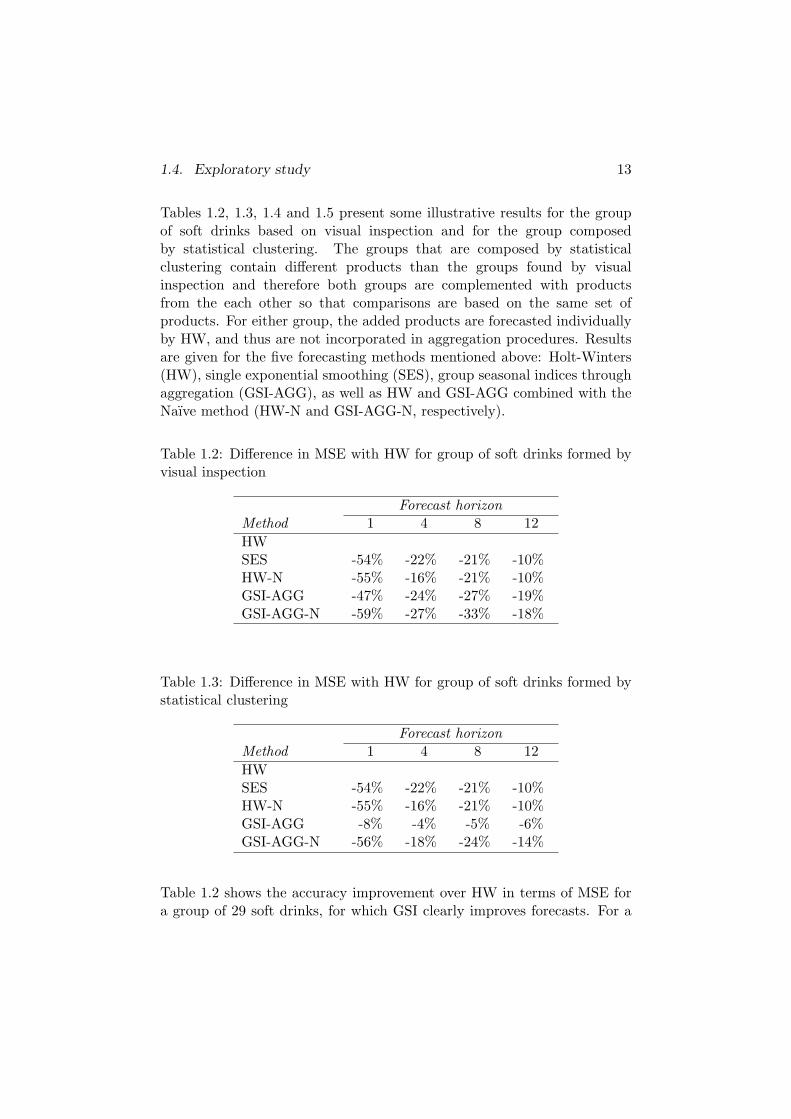
Tables 1.2, 1.3, 1.4 and 1.5 present some illustrative results for the groupof soft drinks based on visual inspection and for the group composedby statistical clustering. The groups that are composed by statisticalclustering contain different products than the groups found by visualinspection and therefore both groups are complemented with productsfrom the each other so that comparisons are based on the same set ofproducts. For either group, the added products are forecasted individuallyby HW, and thus are not incorporated in aggregation procedures. Resultsare given for the five forecasting methods mentioned above: Holt-Winters(HW), single exponential smoothing (SES), group seasonal indices throughaggregation (GSI-AGG), as well as HW and GSI-AGG combined with theNaıve method (HW-N and GSI-AGG-N, respectively).
Table 1.2: Difference in MSE with HW for group of soft drinks formed byvisual inspection
Forecast horizonMethod 1 4 8 12HWSES -54% -22% -21% -10%HW-N -55% -16% -21% -10%GSI-AGG -47% -24% -27% -19%GSI-AGG-N -59% -27% -33% -18%
Table 1.3: Difference in MSE with HW for group of soft drinks formed bystatistical clustering
Forecast horizonMethod 1 4 8 12HWSES -54% -22% -21% -10%HW-N -55% -16% -21% -10%GSI-AGG -8% -4% -5% -6%GSI-AGG-N -56% -18% -24% -14%
Table 1.2 shows the accuracy improvement over HW in terms of MSE fora group of 29 soft drinks, for which GSI clearly improves forecasts. For a

1.4. Exploratory study 14
forecasting horizon of one period ahead the classical Holt-Winters method(HW) performed poorly. Apparently, it has difficulty distinguishing theseasonal pattern from noise. Single exponential smoothing (SES) shows alarge accuracy improvement, but achieves this by choosing a high (close to1) smoothing parameter. It thereby closely follows the actual data and isthus more sensitive to outliers. Compared to HW, both methods HW-Nand GSI-AGG show a large decrease in MSE. The decrease is larger formethod HW-N than for method GSI-AGG. The combination of these twomethods, method GSI-AGG-N, performs best.
For a forecasting horizon greater than one period ahead, the accuracyof HW decreases less than that of other methods, resulting in smallerimprovements of the other methods as the forecast horizon increases.Especially methods that do not incorporate a seasonal pattern (SES) orrely heavily on recent data (HW-N and GSI-AGG-N) rapidly lose theiradded value when forecasting for more distant periods. For GSI-AGG thisdecrease in accuracy improvement is smaller than for other methods, andit remains the best method at longer forecast horizons.
Table 1.4: Average ranks based on MSE for group of soft drinks formed byvisual inspection
Forecast horizonMethod 1 4 8 12HW 1.9 1.8 1.9 1.8GSI-AGG 1.1 1.2 1.1 1.2
Table 1.5: Average ranks based on MSE for group of soft drinks formed bystatistical clustering
Forecast horizonMethod 1 4 8 12HW 1.3 1.3 1.4 1.4GSI-AGG 1.2 1.3 1.1 1.2
The forecast errors (in terms of the different accuracy measures) howeverdo not increase monotonically with increasing lead-time. For some forecast

1.4. Exploratory study 15
horizons the error may even decrease. This is in line with Chatfield andYar (1991), where it was shown that the forecast error variance does notnecessarily increase monotonically with h. This behavior is typical ofnonlinear models (Chatfield, 2000), which multiplicative Holt-Winters is.
Table 1.3 presents results for a group of 16 soft drinks, formed by statisticalclustering, for which GSI-AGG does not give a large accuracy improvement.This shows that the way the products are grouped together can have a largeinfluence on the results, and that a standard statistical clustering methodis not necessarily appropriate. A good statistical cluster (with seasonalpatterns that are very similar) does not necessarily imply that it is optimalfor a group seasonal approach.
Tables 1.4 and 1.5 present the average ranks for these two groups ofproducts, when only HW and GSI-AGG are compared. A value close to 1for either of the methods means that this method is the best method formost of the time series, whereas a value close to 2 means that the othermethod gives better forecasts for most of the time series. In the secondtable, the ranks do not add up to 3 (the sum of the ranks for the twomethods) because the groups were complemented with time series fromeach other, so that we can compare based on the same set of time series.Since these series were not included in the group seasonal procedure, butforecasted individually by HW, a few series scored average rank 1 underboth the GSI and HW methods. In the first table, GSI-AGG takes anaverage rank close to one for all forecast horizons, meaning that GSI-AGGwas best for most time series, whereas in the second table the ranks forboth methods are comparable.
1.4.6 Conclusions
The results presented above are only for a single product category and onlyfor one of the accuracy measures. For this particular group of products, theimprovement in accuracy of GSI-AGG was largest among all product groupsconsidered, and thus gives an indication of the potential improvement thatcan be achieved by adopting a group seasonal approach. Although resultsdiffer per group, the conclusions are similar across the different accuracymeasures.
In general, we can conclude that group seasonality through aggregationcan improve forecast accuracy substantially, both across horizons andacross accuracy measures. Although the advantage of the aggregation

1.4. Exploratory study 16
approach decreases as the horizon increases, accuracy improvementremains. Furthermore, it improves on HW for most time series of allproduct groups, and thus is a robust approach in that sense. However,the way products are grouped is important. The way the group ofproducts is composed has a large influence on the results and a standardclustering algorithm need not be suitable for forming those groups. Finally,aggregation shows potential for both point forecasts and cumulativeforecasts.
The exploratory study shows the potential forecast improvement using agroup seasonal approach. Since these conclusions are specific to the dataused, the rest of dissertation aims at determining more generally whenGSI can improve on HW forecasts. Below in Section 1.4.7 we list somehypotheses on these results.
1.4.7 Hypotheses
Based on the empirical results, three factors that are likely to influencethe effectiveness of GSI are the extent of similarity between the seasonalpatterns, the amount of data available for estimation, and correlationamong items in a group. Below, we formulate several hypotheses on theeffectiveness of GSI that are tested using a simulation study in Chapter 4.
1. The improvement of GSI over HW depends on the variation among theseasonal patterns relative to the random variation
In our exploratory empirical studies, we found that the GSI approachsubstantially improved on HW forecasts when the estimated seasonalpatterns (i.e. the set of seasonal indices) were similar but not identical.Two possible explanations for this are the following:
- The seasonal patterns were in fact the same, but due to large amountsof noise or insufficient data, we were not able to obtain good estimatesof the seasonality, so that the patterns appeared to be different.Because of the noise, GSI helped to improve on HW forecasts. Forgroups of series with little noise, good seasonality estimates couldeasily be obtained, and GSI did not improve accuracy a lot since HWalready performed well.

1.4. Exploratory study 17
- The seasonal patterns were indeed non-identical. The GSI method isrobust to deviations from its underlying model (the data processes forwhich this method is optimal, see Chapter 3) or there are alternativeunderlying models that do not assume identical seasonal patterns. Arationale for the latter would be that even if patterns are only similar,they can still help improve each others estimates since the amount ofdata available is larger.
We are thus interested in determining the extent of similarity requiredfor successful application of GSI. We would like to show whether seasonalpatterns need to be identical or that similarity is sufficient. It is likely thatthis depends on the amount of noise to which the time series are subject.If seasonal patterns are too dissimilar, GSI clearly is not appropriate. Ifthey are identical or only slightly dissimilar, GSI may clearly improve onHW if there is a substantial amount of noise, but not a lot if there is onlylittle noise. Thus, most probably, there is a relation between the two kindsof variation. If there is more variation among the seasonal patterns, thereshould also be more random variation in order for GSI to be more accuratethan HW.
2. GSI improves on the accuracy of HW especially for limited historicaldata
The minimal forecast error that can be obtained for any data process isequal to its noise component. However, due to estimation errors we havelarger errors. With perfect information, such as infinite historical data,however, we could achieve the minimal forecast errors. The added valueof GSI lies in reduction of these estimation errors by using more data inthe form of multiple series. Especially if little historical data is available,obtaining good estimates is difficult. There are only few observations oneach seasonal period and, since seasonal indices are updated only onceevery seasonal cycle, it takes long to improve these estimates. For HWit may take several years to reduce the effect of estimation errors, whilefor GSI more data is readily available. We thus expect that GSI has afaster convergence towards the the minimal forecast error than HW, andespecially under limited historical data reduces estimation errors.
3. GSI is a robust method
From the empirical results it turned out that GSI almost always improved

1.5. Outline of the thesis 18
on HW; it had lower average ranks with lower standard deviations for allforecast horizons. This means that most probably GSI is more accuratethan HW for various data processes. In Chapter 4, we test for two kindsof robustness. Firstly, we investigate whether for deviations from the dataprocesses for which GSI is optimal, GSI is still better than HW. This is doneby looking at the results for the above hypotheses. Secondly, we investigatewhether the GSI and HW methods are insensitive to outliers, by checkingthe amount of variation in their accuracy measures.
4. Negative correlations help GSI to improve on HW
Earlier studies on GSI argue that the reason why this approach works maybe that cross correlations among demands affect the performance (see theliterature review in Chapter 2). We are thus interested in determining underwhich amounts of correlation between the noise processes GSI outperformsHW.
1.5 Outline of the thesis
The remainder of this thesis is organized as follows. In Chapter 2, wereview the literature on hierarchical forecasting, including aggregation-based approaches and studies on group seasonality. Chapter 3 presentsthe statistical framework that specifies the data processes for which GSI isthe optimal forecasting approach. Chapter 4 is dedicated to a simulationstudy that investigates how much accuracy can be improved under variousparameter settings and types of demand patterns. There, we also test thehypotheses from Section 1.4.7. In Chapter 5 we apply the results fromthe simulation study to a set of empirical data. Finally, in Chapter 6 wesummarize the main results of the research and discuss directions for furtherresearch.

Chapter 2
Hierarchical forecasting
In this chapter, we give a review of hierarchical approaches in forecasting.These approaches are aimed at making forecasts for items at various levelsof aggregation where items at lower levels of the hierarchy are membersof the next level in the hierarchy. The levels of a hierarchy can relateto dimensions such as type of products, location, or time. For example,forecasts can be made at the product level or at product family level, perlocation or by region. Also, forecasts can be made for different time spans(a month, a quarter, a year) and for different time buckets (daily, weekly,monthly). In addition to providing forecasts that are consistent at differentlevels of aggregation, hierarchical forecasting has the potential to improveforecast accuracy because it operates on groups of similar time series.
One way to improve accuracy is through aggregation of data. Thiscan mean aggregating the historical data prior to making a forecast, oraggregating the forecasts themselves. The purpose is to use information atone level of aggregation to improve forecasts at another level of aggregation.As mentioned in Chapter 1, hierarchical forecasting includes approachesthat aim at improving estimates by pooling similar time series (such asGSI).
2.1 Hierarchical methods
Aggregation of data can be either across time, called temporal aggregation,or across series, called contemporaneous aggregation. For example, in the
19

2.1. Hierarchical methods 20
contemporaneous dimension, we can make a forecast for a group of itemsinstead of forecasts for items individually. For individual item forecasts, weshould then translate the aggregate forecast back to the disaggregate level.The same ideas can be applied to the temporal dimension. For forecastsfor larger time buckets, we can aggregate the data or forecasts for smallertime buckets. For example, we can forecast at a monthly level instead ofat a weekly level. Data of several time buckets is then aggregated intolarger time buckets. For forecasts for a small time bucket, an aggregation-disaggregation approach can be used: data is aggregated across time, aforecast is made for larger time buckets, and the forecast is translated backto forecasts for the original time buckets.
Our focus here is on the contemporaneous dimension. In contemporaneousaggregation, the data of several time series for each period is aggregatedinto an aggregate series. Several approaches exist that make use of theidea of using data at a higher aggregation level to improve forecasts. Formaking aggregate forecasts, we consider one approach:
- Bottom-up forecasting
For making disaggregate forecasts we discuss two approaches:
- Top-down forecasting
- Group Seasonal Indices
Table 2.1 gives an overview of the most important publications on eachapproach. Although bottom-up and top-down forecasts serve differentpurposes, they are often considered jointly in papers, and are alwayscompared with direct aggregate and disaggregate forecasts, respectively.Group seasonal indices is considered a different topic and is studied inseparate papers. In the following subsections we review the research thathas been done on each of these approaches. The approaches are definedbelow, and summarized in Table 2.2.
Bottom-up (BU)
This approach aims at improving aggregate forecasts. Here, not the actualdata (prior to forecasting) but the forecasts themselves are aggregated inorder to improve a forecast at aggregate level. Some authors (Schwarzkopfet al., 1988; Dangerfield and Morris, 1992), however, refer to forecasts of

2.1. Hierarchical methods 21
Table 2.1: Overview of important publications on hierarchical forecasting
Approach PublicationsBottom-up / Top-down Brown (1962)
Dunn et al. (1976)Miller et al. (1976)Shlifer and Wolff (1979)Barnea and Lakonishok (1980)Wei and Abraham (1981)Schwarzkopf et al. (1988)Gross and Sohl (1990)Dangerfield and Morris (1992)Giesberts (1993)Fliedner (1999)Zotteri and Kalchschmidt (2004)Widiarta et al. (2004a,b,c, 2005)
Group seasonal indices Dalhart (1974)Withycombe (1989)Bunn and Vassilopoulos (1993, 1999)Dekker et al. (2004)Chen (2005)Djajasaputra et al. (2005)This thesis
disaggregate series (without any aggregation) as bottom-up forecasts. Wewill continue with the former definition.
Top-down (TD)
This approach aims at improving forecasts at the disaggregate level, byfirst aggregating the historical data, making a forecast at the aggregatelevel, and then disaggregating the forecast to the level of individualitems. The disaggregation step is usually performed by allocating theaggregate forecast to individual items based on their historical proportionsof aggregate demand. Alternatively, the proportions may be forecast. Grossand Sohl (1990) discuss various ways of determining the proportions.

2.1. Hierarchical methods 22
Group seasonal indices (GSI and GSI-AGG)
Just like the top-down approach, the GSI-AGG method is based onaggregating the data to a level that is higher than that at which a forecastis required, prior to making a forecast. However, this method does notmake a forecast at the aggregate level and so does not have the problemsof disaggregating. Here, the aggregate series is used for obtaining a betterestimate of the seasonal pattern of the individual series. It assumes thatall aggregated items share a common seasonal behavior. The aggregateseries should then make it easier to distinguish the seasonal pattern fromthe noise. The seasonal pattern that is found at the aggregate level is thentransferred to the disaggregate level to improve disaggregate forecasts. Themore general GSI method pools the seasonality estimates from a group ofrelated time series in order to improve the seasonality estimate.
Table 2.2: Overview of approaches
Method Forecast is made for What is aggregatedBottom-up Aggregate level Disaggregate forecastsTop-down Disaggregate level Disaggregate historical dataGSI-AGG Disaggregate level Disaggregate historical data
Whether one should use an aggregation-based approach depends onwhether a forecast from this approach is better than some standard way ofgenerating a forecast. Therefore, we should compare such a derived forecastwith a direct forecast. A direct forecast is defined as a forecast that isonly based on the history (and possibly some additional information) ofthe time series for which a forecast is made. Any forecast that employsdirect forecasts of other time series is a derived forecast. The bottom-up,top-down and GSI approaches are thus all derived. To evaluate a bottom-up forecast, it should be compared with a direct aggregate forecast, whiletop-down and GSI forecasts should be compared with direct disaggregateforecasts.

2.2. Related methods 23
2.2 Related methods
The above approaches are multivariate since they use information fromrelated time series to improve forecasts. Besides these approaches, thereare several other multivariate methods that do not explicitly aggregatedata. Although these methods are not within the scope of this dissertation,we will briefly mention them for sake of completeness. The approachesconsist of models and methods that jointly model the time series, and utilizethe variance-covariance structure between the series to estimate or updateparameters simultaneously. Instead of benefitting from improved datacharacteristics that result from aggregation, they make use of correlationbetween time series directly to improve the estimates of individualparameters or shared characteristics.
For the most common approaches to forecasting (ARIMA, state space,exponential smoothing) such methods or models are available:
- Vector autoregressive (VAR) models, where time series share commonparameters (e.g., Chatfield, 2000)
- Multivariate state space models (e.g., Harvey, 1989), includingBayesian approaches (Pole et al., 1994).
- Multivariate (or vector) exponential smoothing (Jones, 1966; Ennset al., 1982; Harvey, 1986).
- Analogous series. In Duncan et al. (1993, 2001) a Bayesian approachis taken to pooling analogous time series. Parameters estimatedfrom the group model are combined with conventional parameters.Empirical results showed that accuracy can be improved.
Because these methods use the covariance structure between the time series,they can, at least theoretically, make better forecasts than simple BU, TDor GSI approaches. For example, in Wei and Abraham (1981) it is shownthat a joint modeling approach always gives better linear forecasts than aBU approach for weakly stationary series.
2.3 Overview of literature
Most publications establish in what situations or under which conditionsa derived approach is preferred to a direct approach. The outcomes differ

2.3. Overview of literature 24
from paper to paper, depending on the assumptions made. However, nogeneral rule is established. We discuss the assumptions on models andmethods, and the theoretical and empirical results.
Most publications on BU, TD and GSI methods share some commoncharacteristics. Comparisons of methods are based on forecast errorvariance or MSE. Although BU, TD and GSI can be used in combinationwith any forecasting method, most publications discuss this problem usingsmoothing methods. All publications consider the case with only two levelsof hierarchy, usually with only two items.
Several studies that compare direct with derived approaches are empirical(Dunn et al., 1976; Dangerfield and Morris, 1992; Withycombe, 1989;Bunn and Vassilopoulos, 1993, 1999; Dekker et al., 2004). When sucha comparison has been conducted, mostly the scope of the empiricalinvestigations is too limited for general conclusions. Several other studiesassume the underlying data process is known and derive conditions underwhich a derived approach is preferred to a direct one (Shlifer and Wolff,1979; Schwarzkopf et al., 1988; Giesberts, 1993; Zotteri and Kalchschmidt,2004; Widiarta et al., 2004a,b,c, 2005; Chen, 2005). In all cases simplemodels and forecasting methods are used. Only a few papers (Miller et al.,1976; Barnea and Lakonishok, 1980; Wei and Abraham, 1981) derive moregeneral conditions by not assuming a particular data process or forecastingmethod. The conclusions vary somewhat across the papers, but the overallconclusion is that in many cases a direct disaggregate forecast is preferredto a top-down forecast, and a bottom-up forecast is preferred to a directaggregate forecast.
The latter seems counterintuitive, since aggregate data should be easierto forecast. However, at the disaggregate level each individual time seriesmay have a pattern that can be adequately modeled, but aggregating theseprocesses makes the aggregate process too complex to model and forecast.This can be especially apparent if the comparison is based on using thesame forecasting technique at both disaggregate and aggregate level, whichmay not be appropriate. For stationary processes this problem may notarise, but for nonstationary processes essential information may be lostwhen aggregating.
Some publications try to give a general explanation as to why the conceptof aggregation may work. Below, we present the factors that affect theperformance of one method over another. In the next subsections, wediscuss the assumptions and results of all publications in more detail.

2.3. Overview of literature 25
Random fluctuations cancel out
Several authors have argued that forecasts are more accurate for familiesof products. Some argue that forecasts can improve due to the stabilizingeffect from combining demand data (e.g., Muir, 1979). In this case, thecoefficient of variation is smaller for aggregate data than for disaggregatedata. According to this interpretation, aggregation may work even forindependent or slightly positively correlated series. Others argue thatat a higher aggregation level, data shows less variation because randomfluctuations cancel out (e.g., Fliedner, 1999). Some authors are more precisewith respect to this noise reduction.
Miller et al. (1976) and Barnea and Lakonishok (1980) demonstrated forBU that relative forecast performance is dependent on variances of forecasterrors and time series at both aggregate and disaggregate level, as wellas magnitude and sign of cross-correlations between the time series andbetween the forecast errors. Fliedner (1999) carried out a simulation studyand observed that strong positive and strong negative correlation betweenitems improved direct forecasts at the aggregate level. Widiarta et al.(2005), on the other hand, showed in an analytical comparison that fornegative correlations bottom-up forecasts were more accurate than directaggregate forecasts.
For the TD approach, Schwarzkopf et al. (1988) demonstrated thatits accuracy compared to direct disaggregate forecasts depends on thecorrelation between component series, as well as differences between theprocesses and presence of outliers, and provided some situations wherethis is the case. Dangerfield and Morris (1992) used a subset of the M-competition data to examine the effects of cross correlation of the demandsand the item proportion on TD forecasting. They found that directdisaggregate extrapolations for most series resulted in better forecasts thanTD forecasts, and the accuracy improvement was largest when items werehighly negatively correlated and/or when one item dominated the aggregateseries.
More data to estimate certain parameters.
Another argument is that through aggregation, more data is availableto estimate the same parameters, increasing the statistical quality of theestimates. Pooling provides additional data, hereby extending the samplesize (Duncan et al., 2001). Hence pooling should be useful for noisy

2.4. Bottom-up forecasting 26
time series, as measured by the coefficient of variation of deseasonalizedand detrended data. Aggregation reduces the standard error of estimatesbecause more data is available. For example, Zotteri and Kalchschmidt(2004) showed that aggregating stationary data gives a better estimate ofthe mean.
Apart from the above, there are other influential factors that explain whythese aggregation approaches may work. Several publications consider somefactors that may affect the relative performances of alternative approaches.There seem to be two main dimensions with regard to the demand processesthat explain when aggregation approaches work and that are investigated inmost articles. The first dimension concerns dependence and assumes seriesare either independent or dependent to some extent. The second dimensionconcerns similarity and considers whether demand processes are identical(equal means and/or equal variance of noise component) or non-identical.These factors may have opposite effects. Negative item correlation maydecrease variability, favoring aggregate forecast approaches, but also impliesthat the individual processes are different, and thus favoring forecastsat disaggregate level. Conversely, positively correlated series increasesvariability at aggregate level, but may favor an aggregate forecast sincetime series are more similar.
Both Giesberts (1993) and Dangerfield and Morris (1992) consider theimpact of item proportion in the total demand. Shlifer and Wolff (1979)also consider the number of items in a group. Giesberts (1993) derivesunder which conditions direct or derived forecasts are optimal for identicaldemand processes. Wei and Abraham (1981) found that for aggregateforecasts of stationary time series neither a direct or a derived forecastalways has a lower MSE. Rather, particular modeling assumptions, suchas relationships between disaggregate series and parameter estimationprocedures, may lead to favoring one strategy over another. Chen (2005)derives conditions for GSI taking into account the number of items ina group, their means and variances, as well as correlations between thedemand processes.
2.4 Bottom-up forecasting
Bottom-up forecasting is defined in several ways by various authors. Someauthors define it as a forecast of an aggregate series by summing the

2.4. Bottom-up forecasting 27
individual forecasts (Shlifer and Wolff, 1979; Giesberts, 1993; Widiartaet al., 2004a,b,c). Others define it as a forecast at item level (Schwarzkopfet al., 1988; Dangerfield and Morris, 1992). We adopt the former definitionhere. Although the second group of authors mention they compare top-down forecasts with bottom-up forecasts, according to our definition theyare actually comparing with direct disaggregate forecasts.
Most articles derive conditions under which a bottom-up forecast ispreferred to a direct aggregate forecast. They do this for a certain demandmodel, in combination with a specific forecasting method or by assumingthat forecasts are unbiased. Some articles make no assumptions on themodel or method.
In Dunn et al. (1976), empirical data on telephone demand in nine localareas was forecasted by several simple AR models and smoothing methods.Based on MAD and RMSE it was found that bottom-up forecasts resultedin 5-25% accuracy improvement over direct aggregate forecasts.
In Miller et al. (1976) and Barnea and Lakonishok (1980) general theoreticalconditions are derived. No assumptions on the time series models are made,while forecasts are only assumed to be unbiased. Conditions on relativeperformance are obtained given the forecast error variance at aggregateand disaggregate level, and correlation between the disaggregate series andbetween forecast errors of disaggregate variables.
Shlifer and Wolff (1979) derive conditions for demand that is assumed tobe stationary:
yi,t = µi + εi,t (2.1)
for i = 1 . . . n and with εi,t independent and with zero mean and varianceV (εi). While no specific forecasting method is used, one-step aheadforecasts are assumed to be unbiased. The standard deviation of theforecast errors is assumed to have the following functional form:
σi = c + a(µi, h)µb(µi,h)i (2.2)
with h the forecast horizon. For various assumptions on a, b and c,conditions are derived under which either direct or derived forecasts hasa lower forecast error variance. It is the authors’ observation that oftenc = 0, and a and b constant. In this case bottom-up forecasts are preferredwhen b > 1/2.
Wei and Abraham (1981) provide a general result. While only assuming

2.4. Bottom-up forecasting 28
that the component time series are weakly stationary and by restrictingthemselves to linear forecasts, they showed that jointly modeling andforecasting all time series always has a lower MSE for h-step ahead forecaststhan bottom-up or direct aggregate forecasts. However, for the latter two,neither universally outperforms the other.
Giesberts (1993) compares direct aggregate forecasts with bottom-upforecasts. The data is assumed to follow a demand process described by amore general form of the random walk plus noise state space model, referredto in Harvey (1993, p.84) as an AR(1) plus noise process:
yi,t = xi,t + εi,t (2.3a)xi,t = βixi,t−1 + ηi,t (2.3b)
where εi,t and ηi,t are normally distributed and correlated across time series.For each individual time series following this model, an optimal forecast(minimal variance of forecast error) follows from the Kalman filter and isof the exponential smoothing type. A setting with a forecast horizon of oneperiod ahead and two products is considered.
For independent processes, it follows that bottom-up is better than directaggregate forecasting, especially if the difference between the two processesincreases (measured by the difference between the noise variances σε/ση).Only if they are completely identical, both techniques perform equally. Fordependent and identical processes, direct aggregate forecasting is optimal.However, the bottom-up forecast comes closer to the direct aggregateforecast if the correlations between the incidental noise terms (ε1,t andε2,t) or between the changes in systematic pattern (η1,t and η2,t) comecloser to zero, agreeing with the result for independent processes. Fordependent non-identical processes, neither direct aggregate or bottom-upalways performs better. This depends on the extent to which the demandprocesses are dependent and identical. No conditions are derived for thiscase, as opposed to most other articles, where this is the main subject ofstudy.
Fliedner (1999) carried out a simulation study where simple exponentialsmoothing and moving average was used when aggregating two MA(1)processes. It was observed under MAPE that strong positive and strongnegative correlation improved direct forecasts at the aggregate level.
Widiarta et al. (2004a) investigate the BU and the direct aggregateapproach through a simulation study. Demand for families of two

2.5. Top-down forecasting 29
products is generated from four processes: MA(1), AR(1), IMA(1,1), anda stationary process, and is forecasted by single exponential smoothing.An inventory control system is simulated where demand for one item issubstituted by that for the other item if inventory becomes zero. Underthis very specific system, direct aggregate forecasts give better forecaststhan BU forecasts.
Widiarta et al. (2005) give a theoretical analysis for groups of itemsthat follow AR(1) processes and that are forecasted by single exponentialsmoothing. It is shown that the forecast error variances for BU and directaggregate forecasts are the same when the first order autocorrelations of theitem demands are identical. The non-identical case is studied by simulationand it is found that under small or moderate correlation between the itemdemands, there is little difference in forecast accuracy. Only when thecorrelation is highly negative, BU dominates direct aggregate forecasts.
2.5 Top-down forecasting
The top-down strategy makes forecasts of aggregate demand anddistributes this to individual items proportionally. The problem liesin the disaggregation step, where the shares of items can be over orunderestimated, and thus introducing bias at the disaggregate level. Severalways of breaking down the aggregate forecast into item forecasts havebeen suggested. All are in some way based on each item’s share in thefamily demand over some period of time. For examples, we can take thehistorical proportion of total family demand, possibly updated annually.Brown (1962) suggested a vector smoothing method that updates the itemproportions each period before the aggregate forecast is distributed. Grossand Sohl (1990) were the first to systematically examine allocation rulesfor the disaggregation step. They considered 21 different procedures andtested them on empirical data using various forecasting methods. Theresults favored procedures based on a simple average of each item’s shareover the entire historical period.
In Shlifer and Wolff (1979) conditions are derived under which a top-downapproach is preferred to a direct disaggregate forecast. This is done formodel (2.1) under the assumption that forecasts are unbiased and underassumptions on the form of the forecast error. Disaggregation is based onthe estimated value of (µi/
∑ni=1 µi). Especially for items with lower time-

2.5. Top-down forecasting 30
series values, top-down will often result in larger forecast errors becausethe coefficient of variation of the estimated proportions is higher. As thenumber of items in a group increases, direct forecasts are more likely to bepreferred.
Schwarzkopf et al. (1988) consider the following model:
yi,t = pi(Yt + εi,t) (2.4)
with pi the item proportions,∑
pi = 1, εi,t ∼ IID(0, σ2), and Y theaggregate series. They compare, for a family of two items, the meansquared difference between the estimated values of y1 and y2 and the truemean values p1Y and p2Y (instead of the observed values), assuming theproportions pi are known. It was shown that the relative performance ofTD and a direct disaggregate forecast depends on three factors: estimationprecision (variability of the estimate around the predicted value), bias(deviation of the mean of the estimate from the true value), and outlierinfluence (sensitivity to a single bad data point). It was also found thatitem proportions in the aggregate series could have an affect on the relativeperformance of the two techniques. Similar item proportions increases theeffects of model bias and outlier influence when TD is used and thereforefavors direct disaggregate forecasting. However, no specific guidance wasgiven for selecting between the two approaches.
Dangerfield and Morris (1992) carried out an empirical study usingexponential smoothing methods. The two approaches were tested onmore than 15000 families of two items, by taking all possible uniquecombinations of 178 series selected from the M-competition. These seriesdiffered with respect to correlation, seasonal and trend pattern, and theirrelative proportion. The effects of correlation between the two items andthe proportions of individual items in family demand were examined, usingHolt-Winters to make forecasts. The allocation fractions for distributingthe top-down forecasts were equal to the proportion of each item’s demandin the aggregate demand during the estimation period. In most situations(74 %), direct disaggregate forecasts were more accurate than top-downforecasts, with a MAPE that was on average 26% lower than for thetop-down forecast. The influence of item proportion was only small,although one product dominating the aggregate series favored the directdisaggregate approach. Although strong negative correlations would reducevariability in the aggregate series, and thus favor the top-down approach,the direct disaggregate method performed better in this case for 82% of the

2.5. Top-down forecasting 31
series, with a MAPE that was on average 64% smaller. Possibly, negativecorrelation results in reduced variability but also implies that data processesare different. Here, the latter effect may have outweighed the former. ForMSE, results were less pronounced, but more in line with other research.TD showed an improvement only when item proportions were similar, andcorrelations had a much smaller effect on the improvement.
Giesberts (1993) compares Top-down forecasts with direct disaggregateforecasts using state space model (2.3a)-(2.3b) in a setting with two itemsand a forecasting horizon of one period. Similar conclusions as for thebottom-up approach are drawn. Since two independent demand processesdo not give information about each other, direct disaggregate forecasts arealways optimal in that case. For dependent processes, top-down is onlyoptimal for identical processes with full positive correlation between thechanges in the systematic patterns of the two series, implying that aggregatedemand is generated by a common process. This is analyzed by taking theproportions for distributing the aggregate forecast over the individual itemsequal to the ratio of the standard deviations of the changes in systematicpattern (ηi), pi = ση,i/(
∑2i=1 ση,i). For non-identical dependent demand
processes, again neither method always performs better. This depends onthe extent to which the demand processes are dependent and non-identical.No conditions are derived for this case.
Zotteri and Kalchschmidt (2004) provide an analysis for a simple stationaryprocess (i.e., where yi,t = µi + εi,t), leading to a set of conditions underwhich either forecasting alternative is preferred. A top-down approach ispreferred if there is high demand variability, if there are sufficient locations,if demand is homogeneous across locations, or if there is limited historicaldata available. If one or more of these are true, aggregating may improveestimates.
Widiarta et al. (2004c) give a theoretical analysis for groups of itemsthat follow AR(1) processes and that are forecasted by single exponentialsmoothing. It is shown that the forecast error variances for TD anddirect disaggregate forecasts are more or less the same when the first orderautocorrelations of the item demands are small. If at least one item hasa large (> 1/3) autocorrelation, direct disaggregate forecasts outperformTD forecasts, irrespective of the item proportions in family demand andcorrelation between the item demands.
In Widiarta et al. (2004b) a similar analysis is given for a group of itemsfollowing MA(1) processes. Here it is found that the two forecasting

2.6. Group seasonal indices 32
strategies perform nearly the same, regardless of serial correlation,correlation between the items, or item proportions.
2.6 Group seasonal indices
The literature on group seasonal indices is scarce. In the few studiesthat have appeared, the concept is empirically tested (Dalhart, 1974;Withycombe, 1989; Bunn and Vassilopoulos, 1993, 1999) or studiedanalytically (Chen, 2005; Djajasaputra et al., 2005). All empirical studiesshow the improvement potential of product-aggregation over classicalmethods. Nevertheless, they only focus on making short-term forecasts, andthey do not address extensively the issue of how to form product families.Because of the small scale of the comparisons, there is some variation inresults and no general rules can be established.
The analytical study (Chen, 2005) extends the earlier studies bydetermining conditions under which the group seasonal indices methodsof Dalhart (1974) and Withycombe (1989) are more accurate thanconventional seasonal forecasts, based on the following factors: underlyingmeans and variances of disaggregate demands, correlations between thedemands, group size, length of data history, and seasonal length. Theseresults are validated by simulation. All results are for given groups of items,and the issue of forming the groups is not considered. Djajasaputra et al.(2005) presents a state space model that incorporates group seasonality,which is similar in nature as the model that we describe in Chapter 3.
There are some differences in the GSI approaches used in these publications.All studies consider multiplicative seasonality. Although the GSI conceptcan be applied under additive seasonality as well, it is less likely that agroup of products exhibit the same seasonality in absolute sense. OnlyChen (2005) also formulates a method for the additive case.
The way the group seasonal indices are estimated differs from paperto paper. Dalhart (1974) first estimated the seasonal indices for allproducts in a product group individually and then averaged them to obtainthe estimates for the group seasonal indices. These indices were thenused for all items in the group to make forecasts. Withycombe (1989)proposed a different method for calculating the seasonal indices, by firstaggregating the demands for all component series and calculating theseasonal indices at the aggregate level. The improved seasonal estimates

2.6. Group seasonal indices 33
were used to deseasonalize each series in the group, before extrapolation,and to reseasonalize afterwards. Bunn and Vassilopoulos (1993) suggestedto use seasonal indices obtained from Dalhart’s (DGSI), Withycombe’s(WGSI) and the individual seasonal indices method (ISI) methods in severalcombinations for either deseasonalizing or reseasonalizing the data. InBunn and Vassilopoulos (1999) two alternative joint ISI/GSI methods forestimating seasonal indices were considered, namely combining the seasonalindices of ISI, DGSI and WGSI by taking a weighted average of the indicesfrom these methods, and seasonal indices based on shrinkage.
To compute the seasonal estimates, Withycombe (1989) and Bunnand Vassilopoulos (1993, 1999) used ratio-to-moving averages, whileDalhart (1974) simply divided the demand in each period by the annualaverage. After estimating seasonality, in all methods demand is seasonallyadjusted (deseasonalized) and forecasted. Withycombe (1989) and Bunnand Vassilopoulos (1999) use double exponential smoothing, Bunn andVassilopoulos (1993) uses Holt’s two parameter exponential smoothing.Although estimates of level and trend were thus updated by exponentialsmoothing, the seasonal indices were not updated once they were estimated.All methods suggested were tested on simulated or empirical data.
Empirical comparisons
Dalhart (1974) was the first to propose combining products into productclasses to obtain a better estimate of the seasonal component. The conceptwas tested for simulated data for 100 time series and showed substantialimprovements compared to using the individual seasonal indices, althoughno true out-of-sample forecasts were made. In fact, it was only shown thatthe seasonal estimates were more accurate than the individual seasonalestimates.
Although not described explicitly, historical data for 24 periods (t =1, . . . , 24) was generated for the model yi,t = µst + εi,t, where all itemsi = 1, . . . , 100 were assumed to have the same underlying mean µ for allperiods and the same 12 seasonal indices st for (monthly) periods. Theitems differed in the noise component εi,t, which was drawn from a normaldistribution with increasing amplitude from the first to the 100th item. Theseasonal indices were estimated for the first 12 periods, and then multipliedwith the average demand for the next 12 periods. Since this average cannot be known in reality, no proper out-of-sample forecasts were made.

2.6. Group seasonal indices 34
Withycombe (1989) demonstrated the concept for 29 products (6 productclasses with 4 to 6 products) with monthly data from a computerperipherals supplier, and reported an average decrease in total MSE perproduct class of 12% compared to forecasting for individual products. For56% of the forecasts, combining yielded better forecasts. The productclasses were determined by the marketing department, so no groupingprocedure was applied. The first four years of the historical data was usedto compute the seasonal indices (by a ratio-to-moving average procedure)and to compute optimal smoothing parameters. The fifth year was usedfor making twelve one-period ahead forecasts. The aggregated time serieswas calculated by weighting the products by their selling price. The reasongiven for this is that it was assumed that one is usually more concernedwith errors for higher valued products than for low valued ones.
In our analysis we, however, do not consider this option since for expensiveslow moving items, the noise component has too large an influence on theaggregate seasonal pattern. Putting a larger emphasis on higher valuedproducts does not necessarily improve their forecasts. Instead, if one is moreconcerned with the errors of higher valued products, the total accuracy(e.g., the sum of MSE’s) of the forecasts should be weighted.
Bunn and Vassilopoulos (1993) extended the studies of Dalhart andWithycombe by providing a broader comparison of methods and addressingthe issue of forming the groups according to statistical criteria. They usedmonthly data of 54 highly seasonal and slightly trending series from alarge UK department store chain. By clustering, they found 12 groups ofproducts within 5 product classes determined by management. However,they did not provide much detail about the clustering method or the(homogeneity of the) resulting clusters.
GSI, and especially WGSI outperformed the conventional ISI approach.WGSI was found to be most effective for all forecast horizons; itoutperformed other methods most often. It led to an average decreasein MSE (compared to forecasting for individual products) of 6% (averagedover all time series and forecast horizons). Although one, two and three-period ahead forecasts were made, no particular attention was paid to theinfluence of the forecast horizon.
Bunn and Vassilopoulos (1999) used monthly data of 44 highly seasonalseries from a large UK chain of department stores, probably a subset ofthose used in Bunn and Vassilopoulos (1993). The products came from4 business classes, and by clustering 10 groups of products were found

2.6. Group seasonal indices 35
within these classes, and 4 statistical clusters were found within the wholeset of time series. The first two years were used for forming the clustersand deseasonalizing the data, after which forecasts for the third year weremade by Double Exponential Smoothing. The performance of the methodswas compared by computing the MAD, MSE and RMSE, averaged overall time series. It was found that for all accuracy measures and groupingmethods, all GSI methods outperformed ISI. There was no GSI method thatconsistently outperformed the other GSI methods. The statistical clusters(from the whole set of time series) gave the most accurate results.
Benefits of GSI
Dalhart (1974) argued that the benefit is the elimination of noise due toaveraging of the seasonal patterns, and that all items are assumed to have aconsistent underlying seasonal behavior. According to Withycombe (1989),the underlying assumption is that whatever causes the seasonal fluctuationin demand operates the same on all products within the product group. Ifthe assumption is true, then seasonality estimates from the aggregate datashould be better simply by virtue of the cancelation of random variationsin the aggregation.
Seasonal forecasting methods work in situations where the seasonalcomponent is relatively large compared to the noise component, in thosecases they yield improvements in forecast accuracy over non-seasonalmethods. However, if the seasonal component is relatively weak comparedto the random component, these methods may have great difficultydistinguishing the seasonal component from the noise and aggregation mayhelp.
Besides the estimation improvements that can be achieved from aggregatingdata, there are some reasons why this method may yield improved forecaststhat are not explicitly addressed in the literature. An advantage of GSIcompared to the top-down approach is that it avoids bias in the disaggregateforecast since no disaggregation mechanism is needed.
Another advantage is that it increases data availability. Seasonal indicesare revised less frequently than level and trend estimates because newobservations on a particular seasonal index become available only onceevery seasonal cycle. This makes the estimates subject to greater estimationnoise. A group seasonal approach increases the number of observations inthe contemporaneous dimension. The other way round, less data should be

2.6. Group seasonal indices 36
needed for GSI than for ISI to achieve accurate forecasts. GSI thus reducesdata limitations.
Theoretical comparison
Apart from these argued properties, no investigation was undertaken toidentify under what conditions forecasts could be improved. Chen (2005)gives a theoretical comparison of Dalhart’s (DGSI) and Withycombe’s(WGSI) methods with conventional individual seasonal indices forecasting(ISI). Conditions are derived under which each of the methods is preferred,taking into account several factors. To this end, models are considered thatare stationary with either additive or multiplicative seasonality, resultingin a purely additive model,
yit = µi + st + εit, εit ∼ N(0, σ2i ) (2.5)
and a mixed model
yit = µist + εit, εit ∼ N(0, σ2i ) (2.6)
for series i = 1 . . . N . All series are assumed to have a constant meanµi and exactly the same seasonal pattern st. Furthermore, seasonality isassumed to be unchanging from year to year, so that st = st−m, with mthe length of the seasonal cycle. The disturbances are assumed to be onlycross-correlated, with ρij the correlation between εi,t and εj,t. A purelymultiplicative model,
yit = µistεit (2.7)
with lognormal disturbances can be transformed to a purely additive modelwith normal disturbances, and so is not considered further. By applyingthe steps of each method to the model equations, conditions are derived tochoose between ISI, DGSI and WGSI under MSE.
The additive method estimates seasonal factors by dividing eachobservation by the annual mean, and then averaging per factor theestimates obtained from each year. For ISI, this is done on disaggregatedata, for WGSI and DGSI this is done on aggregate data. The seasonalestimates from WGSI need to be disaggregated, by dividing them by N ,and are then equal to estimates from DGSI, which are an average of theindividual estimates. The mean is forecasted by taking a simple average ofall the historical data. Let MSEISI,i and MSEGSI,i be the MSE of ISI and

2.6. Group seasonal indices 37
GSI for series i, respectively. Then for the additive model and method
MSEISI,i −MSEGSI,i =m− 1
T
(σ2
i −σ2
A
N2
)(2.8)
MSEGSI,i < MSEISI,i iff σ2i >
σ2A
N2(2.9)
with T the number of historical periods available and σ2A the variance of
the aggregate series. Since the series are stationary, these MSE’s are validfor all periods in the first full season after the historical data (i.e. forperiods T + 1, . . . , T + m). The equations are independent of the meansµi, and thus only depend on the absolute variance of each time series.The longer the seasonal cycle and/or the shorter the historical estimationperiod, the greater the difference in MSE. When negative correlations arepresent, σ2
A can be lower and more series will benefit from GSI, with greaterimprovements. In other words, a group of time series should be chosenwhere σ2
i −σ2
AN2 is large.
For the mixed model, in combination with the multiplicative method,an analogous analysis is performed, leading to the following approximateresults for DGSI:
MSEISI,i −MSEDGSI,i = (2.10)
m
T
σ2i −
µ2i
N
σ21
µ21
+ . . . +σ2
N
µ2N
+ 2N−1∑j=1
N∑l=j+1
1µj
1µl
ρjlσjσl
MSEDGSI,i < MSEISI,i iff (2.11)
σ2i
µ2i
>1
N2
σ21
µ21
+ . . . +σ2
N
µ2N
+ 2N−1∑j=1
N∑l=j+1
1µj
1µl
ρjlσjσl
MSEISI,i −MSEWGSI,i =m
T
(σ2
i −µ2
i
µ2A
σ2A
)(2.12)
MSEWGSI,i < MSEISI,i iffσ2
i
µ2i
>σ2
A
µ2A
(2.13)

2.7. Overview and research opportunities 38
with µA =∑N
i=1 µi. These results have a similar form as those for theadditive case, but now the item proportions play a role. DGSI or WGSIis better than ISI for a series if the square coefficient of variation is largeenough, i.e. noise series benefit from a GSI approach. Again, under negativecorrelation DGSI or WGSI is more likely to be beneficial. WGSI is betterthan DGSI iff the right-hand side of (2.13) is smaller than that of (2.11),and vice versa. Simulation experiments show that the approximate resultsfor the mixed model are accurate.
The results are empirically tested on data from two companies and representseven groups of between 2 and 66 series, all with monthly data and five yearsof history. Both DGSI and WGSI outperformed ISI under MAD, MSE andsMAPE, while DGSI performed slightly better than WGSI. It was foundthat as the forecasting horizon increases, the benefit of using GSI decreases.This is in line with the results presented in Chapter 1. However, the lengthof historical data did not affect the results. Apparently, both ISI and GSImethods benefitted equally from more data to obtain estimates.
State space approach
Whereas the above papers have a focus on forecasting methods,Djajasaputra et al. (2005) presents a multivariate state space model thatdescribes a group of time series that share a group seasonal pattern. Themodel is an extension of the Basic Structural Model (Harvey, 1989) in whichthe time series share a common seasonal component. This model can beestimated and forecasted by an updating procedure in which data is notaggregated as in the above articles. Application of the updating procedureto empirical data show that it leads to improved accuracy.
The main distinction with the articles discussed above and the research inthis thesis, is that this article assumes seasonality is additive. As mentionedabove, it may be difficult to find a group of time series that have the sameadditive seasonal component. However, purely multiplicative data (as inmodel 2.7) can be transformed to purely additive data.
2.7 Overview and research opportunities
Although the above studies have shown that there is a potential value ofGSI methods, none of the studies are complete, and thus leave some gaps
2.7. Overview and research opportunities 39
to be filled. Based on the above literature, some topics arise for furtherresearch.
Especially the earlier studies (Dalhart, 1974; Withycombe, 1989; Bunn andVassilopoulos, 1993, 1999) show limited empirical results. In Chapter 1, wehave provided a more extensive empirical comparison, including more dataand more types of forecasts and forecast horizons. The main conclusionfrom all studies is that a GSI approach potentially leads to improvedforecast accuracy. However, there is a large variation in the size of theimprovement, even within the results from a particular publication. Insome cases it works, in other cases it does not. Therefore it is difficultto draw general conclusions. In order to successfully apply GSI and toguarantee that it works for a given group of products, however, generalrules must be derived.
Some factors have been identified that influence results. The mainfactors that determine whether TD/BU/GSI is better are the variancesof the demands, correlation between demand, the item proportions, groupsize, length of data history and seasonal cycle, and forecast horizon.Also, publications on top-down and bottom-up forecasting suggest thataggregating should only be done for a group of homogeneous time series.The publications on GSI are based on the assumption of a commonseasonality for all items in a group. The question is how homogeneousa group should be and how these group should be formed. All publicationsassume that a group of items is given and acknowledge that it is difficultto establish whether a group of items has a common seasonal pattern, butprovide no solution to form groups.
There is some difference in the GSI methods in the publications. Thereare differences in the way the group seasonal patterns are estimated, andin how forecasts are actually made. In the methods studied in Dalhart(1974), Withycombe (1989), Bunn and Vassilopoulos (1993) and Bunn andVassilopoulos (1999), once the seasonal indices are computed, they are notupdated any more as new data becomes available. This is only reasonableif the seasonal patterns are assumed not to change over time. However,using exponential smoothing for forecasting implies that deseasonalizeddemand is assumed to change over time, which is unlikely if seasonalityis deterministic.
When GSI is studied more theoretically, several models are assumed. Itis for example assumed that the underlying means and seasonal patternsare unchanging. The assumptions allow the analysis to remain simple.

2.7. Overview and research opportunities 40
In this way, estimation of the seasonal component from either individualor aggregate time series is compared. Simplifying assumptions are madefor the rest of the forecasting process, and no updating procedure isincorporated. This is done because for more complex assumptions andforecasting procedures, the models are no longer tractable. Another issueis that the form of the models is not necessarily such that we would applythe ISI or GSI methods in the first place. If all time series components arefixed, a regression approach might be more appropriate. The methods arestudied without knowing for what data generating processes the methodsare optimal or at least suitable.

Chapter 3
Theoretical framework forGroup Seasonal Indices
Part of the content of this chapter appears in Ouwehand et al. (2006)
3.1 Introduction
In this chapter, we develop a theoretical framework for the group seasonalindices approach. In Section 1.4, we proposed a method that aggregatesdata in order to improve seasonal forecasts. The approach updates leveland trend components at the item level, while the seasonal componentis updated at the aggregate level. Empirical results were favorable forthis method, but it was not clear when it improved on conventional Holt-Winters forecasts. In this chapter, we identify data processes for whichthis method is the best method. This is done by developing an underlyingmodel. An underlying model is a model for which a particular method isoptimal. That is, for data that behaves according to the underlying model,the method generates forecasts with a minimal Mean Squared Error (MSE).We look at models where all time-series components are assumed to beonly locally constant. That is, they may change from period to period.The model developed is a generalization of the models underlying the Holt-Winters method, as described in Ord et al. (1997) and Koehler et al. (2001).It is an underlying model for the GSI procedure, which is a generalizationof the Holt-Winters procedure. The model underlies a method that poolsthe time series to improve forecasts. This method is more general than the
41

3.2. Underlying models for exponential smoothing 42
method that aggregates the time series, and the latter is thus a special case.Since the GSI approach bears a close relation with exponential smoothing,in particular Holt-Winters, we first discuss the models underlying the mostcommon exponential smoothing methods. After that, we present the modelunderlying the GSI approach.
When we consider underlying models for a forecasting method, we meanthat the optimal prediction given by the forecasting method is the sameas the one computed by taking the conditional expectation of a futurevalue for the underlying model given past values. This implicitly assumesa quadratic loss function and gives minimum MSE forecasts conditional onthe model. The reason for this is that the conditional expectation of yt+h
is the minimum mean square error estimator (MMSE) of yt+h. Thus, aminimal MSE forecast is obtained by taking taking the forecast yt(h) (oryt+h|t) equal to the expected value of yt+h conditional on the informationavailable at time t, Yt = {yt, yt−1, ...}, i.e. by taking yt(h) = E(yt+h|Yt).See Harvey (1989) for a proof of this.
3.2 Underlying models for exponential smoothing
Exponential smoothing methods were long seen as ad hoc methods,lacking a statistical basis. They were intuitively sensible, but were simpleoperational procedures originating from practice. Some forms could beconsidered a special case of ARIMA modeling (Box et al., 1994). However,recent research (Ord et al., 1997; Hyndman et al., 2002) has changed thisview and now it is known that exponential smoothing methods are optimalfor a class of state space models that is broader than the ARIMA class.
The class of state space models has proven to be suitable for modelingexponential smoothing. State space models cover a wide range of models.For example, unobserved components models, Harvey’s (1989) structuralmodels, and dynamic linear models used in Bayesian forecasting (Pole et al.,1994), are all state space representations. Furthermore, many models,including ARIMA and ordinary linear regression models, can be writtenin state space form. State space models are appealing since they modelall time series components (level, trend, seasonality) explicitly, and can bewritten in a form that is similar to the corresponding exponential smoothing

3.2. Underlying models for exponential smoothing 43
method. The general univariate linear state space model is given by
yt = h′tθt + εt (3.1a)
θt = Gtθt−1 + ηt (3.1b)
for t = 1, . . . , T , where yt is the observed time series value. ht (withh′
t its transpose) is assumed to be a known (k × 1) vector, Gt a known(k × k) matrix and θt is the (possibly unobservable) (k × 1) state vector.Furthermore, εt are serially uncorrelated disturbances assumed to havezero mean and variance σ2
ε , while ηt is a vector of serially uncorrelateddisturbances with zero mean and covariance matrix Wt. Usually, εt andηt are assumed to be (multivariate) normally distributed and uncorrelatedwith each other at all time periods (i.e. E(εtηs) = 0 for all t, s = 1, ..., T ).The model is thus characterized by ht, Gt, σ2
ε and Wt. Equation (3.1a) isknown as the observation equation and (3.1b) as the transition equation.If ht, Gt, σ2
ε and Wt do not change over time, the model is said to be time-invariant. For the principal exponential smoothing variants, the underlyingstate space models are time-invariant.
Since state space models contain both an unobservable state vector andunknown parameters, estimation for state space models has two aspects:
- Estimating the unknown parameters
- Estimating the unobservable state variables
The first can be done by, for example, maximum likelihood estimation.The second is done by the Kalman filter (see e.g., Harvey, 1989). TheKalman filter is a recursive procedure for computing the optimal estimatorof the state vector at time t, based on the information available at time t(i.e. the observations up to and including yt). Every time period, whennew observations become available, this information is used to updatethe estimates. For state space models, optimal predictions of futureobservations and optimal estimates of unobserved components can be madeusing the Kalman filter. If the model is Gaussian (εt, ηt and the initial stateare normally distributed), the Kalman filter is optimal in the sense that ityields minimum mean square error estimators (MMSE’s).
A special form of the state space model is the innovations model of

3.2. Underlying models for exponential smoothing 44
Anderson and Moore (1979):
yt = h′tθt−1 + εt (3.2a)
θt = Tθt−1 + αεt (3.2b)
with θt the (k×1) state vector, ht a (k×1) vector of coefficients, T a (k×k)transition matrix, and α a fixed (k × 1) vector. The difference with thegeneral state space model (3.1a)-(3.1b) is that the disturbance terms in theobservation and transition equations are now perfectly correlated, implyingthat there is effectively only a single source of randomness. Since there isonly one disturbance term in the model, it is referred to as a single sourceof error (SSOE) model. Models with more than one disturbance term areknown as multiple sources of error (MSOE) models. This model has manycommon models as special cases, such as multiple regression, exponentialsmoothing, and ARIMA models. Any ARIMA model can be converted tothis form. This model was first related to exponential smoothing in Snyder(1985), and an SSOE model also forms the basis for the model underlyingGSI.
For both the time-invariant MSOE and SSOE model, the Kalman filterconverges to a steady state under some conditions. As the number ofobservations increases a set of fixed updating equations result. For somemodel forms, exponential smoothing equations follow. This implies that theexponential smoothing equations can only be used when this convergencetakes place at a reasonable rate. Some simulation results in Ord et al.(2005), however, show that this convergence is exponentially fast.
Table 3.1 gives an overview of the main underlying models for the mostcommon exponential smoothing methods, consisting of ARIMA models andboth SSOE and MSOE state space models. It lists underlying models forsingle exponential smoothing (SES), Holt’s exponential smoothing (HES),additive Holt-Winters (AHW) and multiplicative Holt-Winters (MHW).
Muth (1960) was the first to provide a statistical model for SES, namelythe random walk plus noise model.
yt = lt + εt (3.3a)lt = lt−1 + ηt (3.3b)
where εt ∼ NID(0, σ2ε) and ηt ∼ NID(0, σ2
η), and εt and ηt are mutuallyand serially independent. By e.g., applying the Kalman filter, it can

3.2. Underlying models for exponential smoothing 45
Table 3.1: Overview of methods and models considered
Method Underlying modelsSES Random walk plus noise, MSOE and SSOE
ARIMA(0,1,1)HES Linear growth model, MSOE and SSOE
ARIMA(0,2,2)AHW Basic structural model, MSOE and SSOE
SARIMA(0, 1,m + 1)(0, 1, 0)m
MHW Dynamic nonlinear model, MSOE and SSOE
be shown that SES is a minimum mean squared error forecast with αdetermined by the ratio of the variances of the noise processes. The SSOEvariant of this model,
yt = lt−1 + εt (3.4a)lt = lt−1 + αεt (3.4b)
where εt ∼ NID(0, σ2ε) and serially independent, appears to result in SES
forecasts as well. This model can easily be rewritten as an ARIMA(0,1,1)model, for which SES thus also produces optimal forecasts. In case boththe level and growth rate are changing, Holt’s method is optimal for thelinear growth model (Theil and Wage, 1964):
yt = lt + εt (3.5a)lt = lt−1 + bt + η1,t (3.5b)bt = bt−1 + η2,t (3.5c)
with normally distributed and independent error terms. The optimalsmoothing parameters are determined by the relative variances of thethree white noise processes. The SSOE variant of this model and theARIMA(0,2,2) process also result in forecasts from Holt’s method.
This model can be extended with an additive seasonal component, resultingin the Basic Structural Model (Harvey, 1989), for which the Kalman filterconverges to the updating equations of additive Holt-Winters. Furthermore,additive Holt-Winters is also optimal for a seasonal ARIMA model, whichcan be obtained from the Basic Structural Model. This model is known as

3.3. Model for GSI 46
the SARIMA(0, 1,m + 1)(0, 1, 0)m model (Roberts, 1982), and is basicallyan ARIMA(0, 1,m + 1) model extended with a seasonal part, where(0, 1, 0)m denotes taking seasonal differences of order m.
3.3 Model for GSI
Since the GSI approach bears a close relation with the Holt-Wintersmethod, we first discuss the models underlying this method. Since thismethod is nonlinear, there will not be an ARIMA model underlying thismethod (since these are inherently linear). However, the class of state spacemodels has provided a way to underpin this method. Since the models arealso nonlinear, the standard Kalman filter does not apply. Nonlinear statespace models (dynamic nonlinear models) with multiple sources of error areusually estimated using quasi-maximum likelihood methods in conjunctionwith an extended Kalman filter.
In Ord et al. (1997) a class of nonlinear state space models is introduced thathave only one disturbance term. These simpler models can be estimatedby a conditional maximum likelihood procedure based on exponentialsmoothing instead of an extended Kalman filter. One of the models in thisclass is the model underlying the multiplicative Holt-Winters procedure.The minimum mean square error updating equations and forecast functionfor this model correspond to those of the HW method. The model is basedon two ideas:
- A single source of error (Snyder, 1985)
- A multiplicative error term (Ord and Koehler, 1990)
The characteristics of this model are summarized below.
3.3.1 Univariate MSOE model
In Ord and Koehler (1990) a multiplicative alternative to the (additive)basic structural model (Harvey, 1989) was proposed, where the error
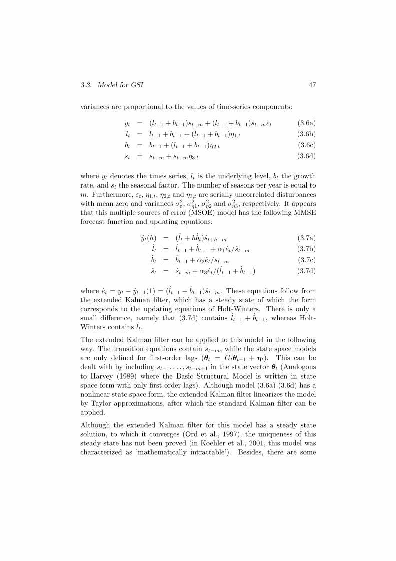
3.3. Model for GSI 47
variances are proportional to the values of time-series components:
yt = (lt−1 + bt−1)st−m + (lt−1 + bt−1)st−mεt (3.6a)lt = lt−1 + bt−1 + (lt−1 + bt−1)η1,t (3.6b)bt = bt−1 + (lt−1 + bt−1)η2,t (3.6c)st = st−m + st−mη3,t (3.6d)
where yt denotes the times series, lt is the underlying level, bt the growthrate, and st the seasonal factor. The number of seasons per year is equal tom. Furthermore, εt, η1,t, η2,t and η3,t are serially uncorrelated disturbanceswith mean zero and variances σ2
ε , σ2η1, σ2
η2 and σ2η3, respectively. It appears
that this multiple sources of error (MSOE) model has the following MMSEforecast function and updating equations:
yt(h) = (lt + hbt)st+h−m (3.7a)lt = lt−1 + bt−1 + α1et/st−m (3.7b)bt = bt−1 + α2et/st−m (3.7c)st = st−m + α3et/(lt−1 + bt−1) (3.7d)
where et = yt − yt−1(1) = (lt−1 + bt−1)st−m. These equations follow fromthe extended Kalman filter, which has a steady state of which the formcorresponds to the updating equations of Holt-Winters. There is only asmall difference, namely that (3.7d) contains lt−1 + bt−1, whereas Holt-Winters contains lt.
The extended Kalman filter can be applied to this model in the followingway. The transition equations contain st−m, while the state space modelsare only defined for first-order lags (θt = Gtθt−1 + ηt). This can bedealt with by including st−1, . . . , st−m+1 in the state vector θt (Analogousto Harvey (1989) where the Basic Structural Model is written in statespace form with only first-order lags). Although model (3.6a)-(3.6d) has anonlinear state space form, the extended Kalman filter linearizes the modelby Taylor approximations, after which the standard Kalman filter can beapplied.
Although the extended Kalman filter for this model has a steady statesolution, to which it converges (Ord et al., 1997), the uniqueness of thissteady state has not been proved (in Koehler et al., 2001, this model wascharacterized as ’mathematically intractable’). Besides, there are some

3.3. Model for GSI 48
other disadvantages of this model, given in Ord et al. (1997): i) Thisapproach involves greater levels of approximation when the equations arelinearized in order to apply the extended Kalman filter. The SSOE modelbelow does not have this problem. ii) This approach is not applicable fornonnormal error distributions.
3.3.2 Univariate SSOE model
The combination of a single source of error (SSOE) and a multiplicativeerror term led to the model proposed in Ord et al. (1997). This modelhas a single source of error describing the development of all time seriescomponents, in combination with multiplicative error terms, and is specifiedby
yt = (lt−1 + bt−1)st−m + (lt−1 + bt−1)st−mεt (3.8a)lt = lt−1 + bt−1 + α1(lt−1 + bt−1)εt (3.8b)bt = bt−1 + α2(lt−1 + bt−1)εt (3.8c)st = st−m + α3st−mεt (3.8d)
In fact, there are several models for which multiplicative Holt-Winters isoptimal (Koehler et al., 2001). These are all special cases of the generalmodel that is defined by
yt = (lt−1 + bt−1)st−m + (lt−1 + bt−1)βsγt−mεt (3.9a)
lt = lt−1 + bt−1 + α1(lt−1 + bt−1)βsγ−1t−mεt (3.9b)
bt = bt−1 + α2(lt−1 + bt−1)βsγ−1t−mεt (3.9c)
st = st−m + α3(lt−1 + bt−1)β−1sγt−mεt (3.9d)
with 0 ≤ β, γ ≤ 1. By letting both β and γ be either 0 or 1, four differentmodels arise that have a one-step ahead prediction error variance that isconstant or proportional to level and/or seasonal index. The choice of theerror variation does not affect the form of the updating equations, theseare the same for all four models (although parameter estimates will bedifferent). However, it does have an effect on the variance structure of theforecast errors and thus on prediction intervals. Solving the measurementequation for εt and substituting for εt in the transition equations gives the

3.3. Model for GSI 49
error-correction form for these models:
lt = lt−1 + bt−1 + α1et/st−m (3.10a)bt = bt−1 + α2et/st−m (3.10b)st = st−m + α3et/(lt−1 + bt−1) (3.10c)
with et = yt − (lt−1 + bt−1)st−m. The initial states l0, b0 and s−m+1, . . . , s0
have to be estimated by l0, b0 and s−m+1, . . . , s0, after which consecutiveestimates of lt, bt and st can be calculated from these formulae. Afterestimation, the transition equations show great similarity with the error-correction form of classical multiplicative Holt-Winters:
yt(h) = (lt + hbt)st+h−m (3.11a)lt = lt−1 + bt−1 + αet/st−m (3.11b)bt = bt−1 + αβet/st−m (3.11c)st = st−m + γ(1− α)et/lt (3.11d)
The only difference is the denominator on the right-hand side of theupdating equation for the seasonal indices, but since lt ≈ lt−1 + bt−1, thedifference is only minor. In Chapter 4, we present some simulation resultsthat confirm that this is indeed the case.
3.3.3 Development of model
In this section, we discuss some preliminary GSI methods and theirunderlying models that led to the model and method presented in thenext subsection. Each combination of model and method itself is notsuitable for GSI, but has elements that are important to find an underlyingmodel for GSI. All models differ with respect to the data processes theydescribe and their optimal methods, but have the same forecast function.A forecast for item i for h steps ahead, made at time t is given byyi,t(h) = (li,t + hbi,t)st+h−m.
Alternative 1
The empirical studies presented in Section 1.4 were based on a methodwhere level and trend components are updated at the disaggregate level
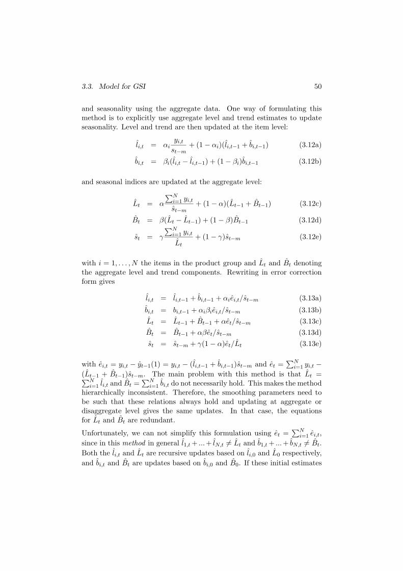
3.3. Model for GSI 50
and seasonality using the aggregate data. One way of formulating thismethod is to explicitly use aggregate level and trend estimates to updateseasonality. Level and trend are then updated at the item level:
li,t = αiyi,t
st−m+ (1− αi)(li,t−1 + bi,t−1) (3.12a)
bi,t = βi(li,t − li,t−1) + (1− βi)bi,t−1 (3.12b)
and seasonal indices are updated at the aggregate level:
Lt = α
∑Ni=1 yi,t
st−m+ (1− α)(Lt−1 + Bt−1) (3.12c)
Bt = β(Lt − Lt−1) + (1− β)Bt−1 (3.12d)
st = γ
∑Ni=1 yi,t
Lt
+ (1− γ)st−m (3.12e)
with i = 1, . . . , N the items in the product group and Lt and Bt denotingthe aggregate level and trend components. Rewriting in error correctionform gives
li,t = li,t−1 + bi,t−1 + αiei,t/st−m (3.13a)
bi,t = bi,t−1 + αiβiei,t/st−m (3.13b)Lt = Lt−1 + Bt−1 + αet/st−m (3.13c)Bt = Bt−1 + αβet/st−m (3.13d)st = st−m + γ(1− α)et/Lt (3.13e)
with ei,t = yi,t − yt−1(1) = yi,t − (li,t−1 + bi,t−1)st−m and et =∑N
i=1 yi,t −(Lt−1 + Bt−1)st−m. The main problem with this method is that Lt =∑N
i=1 li,t and Bt =∑N
i=1 bi,t do not necessarily hold. This makes the methodhierarchically inconsistent. Therefore, the smoothing parameters need tobe such that these relations always hold and updating at aggregate ordisaggregate level gives the same updates. In that case, the equationsfor Lt and Bt are redundant.
Unfortunately, we can not simplify this formulation using et =∑N
i=1 ei,t,since in this method in general l1,t + ...+ lN,t 6= Lt and b1,t + ...+ bN,t 6= Bt.Both the li,t and Lt are recursive updates based on li,0 and L0 respectively,and bi,t and Bt are updates based on bi,0 and B0. If these initial estimates

3.3. Model for GSI 51
are estimated through separate estimation procedures,∑N
i=1 li,0 and L0 willbe different, as will
∑Ni=1 bi,0 and B0. Only if L0 =
∑Ni=1 li,0, B0 =
∑Ni=1 bi,0
and all αi and α as well as all βi and β are the same, we are guaranteed tohave Lt =
∑Ni=1 li,t and Bt =
∑Ni=1 bi,t.
In a model on the other hand, the error at aggregate level can beexpressed in terms of the disaggregate error components, by assumingLt =
∑Ni=1 li,t−1 and Bt =
∑Ni=1 bi,t−1. But, if we simplify a model in this
way, it will be impossible to find the method in equations (3.18a)-(3.18c)as a result of the model.
Alternative 2
A second alternative formulation of the GSI method is the following:
li,t = αiyi,t
st−m+ (1− αi)(li,t−1 + bi,t−1) (3.14a)
bi,t = βi(li,t − li,t−1) + (1− βi)bi,t−1 (3.14b)
st = γ
∑Ni=1 yi,t∑Ni=1 li,t
+ (1− γ)st−m (3.14c)
Rewriting this in error-correction form yields
li,t = li,t−1 + bi,t−1 + αiei,t/st−m (3.15a)
bi,t = bi,t−1 + αiβiei,t/st−m (3.15b)
st = st−m + γ
∑Ni=1(1− αi)ei,t∑N
i=1 li,t(3.15c)
The underlying model that can be derived from this,
yi,t = (li,t−1 + bi,t−1)st−m + (li,t−1 + bi,t−1)st−mεi,t (3.16a)li,t = li,t−1 + bi,t−1 + αi(li,t−1 + bi,t−1)εi,t (3.16b)bi,t = bi,t−1 + αiβi(li,t−1 + bi,t−1)εi,t (3.16c)
st = st−m + st−m
∑Ni=1(1− αi)(li,t−1 + bi,t−1)εi,t∑N
i=1(li,t−1 + bi,t−1)(3.16d)

3.3. Model for GSI 52
yields the following updating equations in error-correction form:
li,t = li,t−1 + bi,t−1 + αiei,t/st−m (3.17a)bi,t = bi,t−1 + αiβiei,t/st−m (3.17b)
st = st−m +∑N
i=1(1− αi)ei,t∑Ni=1(li,t−1 + bi,t−1)
(3.17c)
corresponding to the error-correction form of method (3.15a)-(3.15c) (witha minor difference, since li,t is replaced by li,t−1 + bi,t−1 ). However, thismethod uses the same αi’s to smooth both level and seasonality, implyingthat higher variability in the level would mean lower variability in theseasonality. It is appropriate to have separate parameters for each of thecomponents.
Alternative 3
If we define an error-correction form with separate parameters for each ofthe components
li,t = li,t−1 + bi,t−1 + αiei,t/st−m (3.18a)
bi,t = bi,t−1 + αiβiei,t/st−m (3.18b)
st = st−m + γ(1− α)∑N
i=1 ei,t∑Ni=1 li,t
(3.18c)
this results in a recurrence form for the GSI method of the following form
li,t = αiyi,t
st−m+ (1− αi)(li,t−1 + bi,t−1) (3.19a)
bi,t = βi(li,t − li,t−1) + (1− βi)bi,t−1 (3.19b)
st = δ
∑Ni=1 yi,t + (li,t − li,t−1 − bi,t−1)st−m∑N
i=1 li,t+ (1− δ)st−m (3.19c)
with δ = γ(1 − α). The following model is an underlying model for this

3.3. Model for GSI 53
method:
yi,t = (li,t−1 + bi,t−1)st−m + (li,t−1 + bi,t−1)st−mεi,t (3.20a)li,t = li,t−1 + bi,t−1 + α1i(li,t−1 + bi,t−1)εi,t (3.20b)bi,t = bi,t−1 + α2i(li,t−1 + bi,t−1)εi,t (3.20c)
st = st−m + α3st−m
∑Ni=1(li,t−1 + bi,t−1)εi,t∑N
i=1(li,t−1 + bi,t−1)(3.20d)
By rewriting in error-correction form, the model has the following updatingequations:
li,t = li,t−1 + bi,t−1 + α1iei,t/st−m (3.21a)bi,t = bi,t−1 + α2iei,t/st−m (3.21b)
st = st−m + α3
∑Ni=1 ei,t∑N
i=1(li,t−1 + bi,t−1)(3.21c)
with ei,t = yi,t − (li,t−1 + bi,t−1)st−m. This corresponds to the updatingequations of the method in (3.18a)-(3.18c) (with a minor difference).Although the model seems sensible, the problem with the method is thatthe seasonal equation (3.19c) does not aggregate data by simple summingup the time series, it incorporates a slight adjustment to the yi,t beforedividing by
∑Ni=1 li,t.
Conclusion
From the above, it appears that it is difficult to find an underlying modelfor the GSI-AGG method that we used in Chapter 1. That method isa generalization of the classical Holt-Winters method, and the seasonalupdating equation thus contains li,t in the denominator. An underlyingmodel for a method with this characteristic always has some problems, asexplained for the three alternatives above.
In this subsection, we have seen that an underlying model for GSI should beconsistent among the hierarchies, use different parameters for each of thecomponents, and use li,t−1 + bi,t−1 instead of li,t−1 to update the seasonalestimates. In the next subsection, we show that, by allowing the method tocontain li,t−1 + bi,t−1, a consistent combination of method and underlyingmodel can be found.

3.3. Model for GSI 54
3.3.4 Multivariate SSOE model
The following model underlies the GSI approach:
yi,t = (li,t−1 + bi,t−1)st−m + (li,t−1 + bi,t−1)st−mεi,t (3.22a)li,t = li,t−1 + bi,t−1 + αi(li,t−1 + bi,t−1)εi,t (3.22b)bi,t = bi,t−1 + αiβi(li,t−1 + bi,t−1)εi,t (3.22c)
st = st−m + γst−m
N∑i=1
wiεi,t (3.22d)
with i = 1, . . . , N the items in the product group and li,t and bi,t denotingtheir level and trend components. All items share a common seasonality,denoted by st. All items have normally distributed disturbances εi,t. Thewi are weights with
∑Ni=1 wi = 1. This model can be rewritten in error-
correction form as
li,t = li,t−1 + bi,t−1 + αiei,t/st−m (3.23a)bi,t = bi,t−1 + αiβiei,t/st−m (3.23b)
st = st−m + γN∑
i=1
wiei,t
li,t−1 + bi,t−1(3.23c)
with ei,t = yi,t − (li,t−1 + bi,t−1)st−m. The minimal MSE method resultingfrom this model has the following updating equations:
li,t = αiyi,t
st−m+ (1− αi)(li,t−1 + bi,t−1) (3.24a)
bi,t = βi(li,t − li,t−1) + (1− βi)bi,t−1 (3.24b)
st = γN∑
i=1
wiyi,t
li,t−1 + bi,t−1
+ (1− γ)st−m (3.24c)
A h-step ahead forecast for item i, made at time t, is given by yi,t(h) =(li,t +hbi,t)st+h−m. To see why this model indeed yields these equations forforecasts and updates of state variables, first consider the SSOE version ofthe random walk plus noise model:
yt = lt−1 + εt (3.25a)lt = lt−1 + αεt (3.25b)

3.3. Model for GSI 55
Solving the first equation for εt and substituting in the second one gives
lt = αyt + (1− α)lt−1 (3.26)
which can be further worked out to lt = (1−α)tl0+α∑t−1
j=0(1−α)jyt−j . Theconsecutive values of the lt are thus determined by a starting value l0 andthe observations y1, y2, . . . . This means that once we have an estimate forl0, namely l0, subsequent estimates l1, l2, . . . can easily be computed everyperiod as new observations become available. In other words, an estimatefor lt can be computed by taking its conditional expectation, given thechoice of the starting value and parameters, and the observations:
lt = E(lt|l0, α, y1, . . . , yt) (3.27)
Since all necessary quantities are known, no actual expectation has to betaken and lt can simply be computed using recursion (3.26). In this way,we get minimum mean square error estimates of the lt’s, conditional onl0. A minimum mean square error forecast is then obtained by taking theconditional expectation of (3.25a), E(yt+h|l0, α, y1, . . . , yt) = lt.This idea extends to the model for GSI. The error-correction form in(3.23a)-(3.23c) is the equivalent of that for the random walk plus noisemodel in (3.26). Again, once starting values li,0, bi,0 and s−m+1, . . . , s0 havebeen provided, subsequent estimates of li,t, bi,t and st can be calculated asobservations become available. The forecast function is equal to
E(yi,t+h|li,0, bi,0, s−m+1, . . . , s0, α1i, α2i, α3, yi,1, . . . , yi,t) (3.28)
= (li,t + hbi,t)st+h−m
The initial states and the smoothing parameters can be estimated by forexample using a maximum likelihood approach, or by minimizing someother criterion such as MSE.
3.3.5 Pooling seasonal estimates
The method (3.24a)-(3.24c) resulting from model (3.22a)-(3.22d) is ageneralization of the Holt-Winters procedure (3.11a)-(3.11d). The updatingequations for level and trend are the same as those for HW. The updatingequation for the seasonal component, however, makes use of all time seriesi = 1, . . . , N . It updates the previous estimate st−m by weighting it with a

3.3. Model for GSI 56
new estimate∑N
i=1wiyi,t
li,t−1+bi,t−1. This new estimate is a weighted average of
N estimates obtained from all time series independently. By pooling theseestimates using weights wi, the forecast accuracy can be improved.
The weights wi can be chosen to minimize forecast errors, measured byfor example MSE, or can be specified in a variety of other ways. Forexample, taking wi = 1
N gives equal weight to all error terms and thus alltime series. Taking a simple average means all time series are considered tohave the same amount of noise and thus get the same smoothing parameterγ 1
N . If this is not the case, highly variable series may corrupt the estimatedseasonal component. In general, noisier series should thus get lower weights.The lower the relative noise εi,t, the higher the weight wi should be, andthus also the higher the smoothing parameter γwi should be.
The variability of a time series can be measured by the variance of relativenoise, equal to V ar( ei,t
(li,t−1+bi,t−1)st−m) = V ar(εi,t) = σ2
i , or by the coefficientof variation of deseasonalized and detrended data, y′i,t = yi,t
(li,t−1+bi,t−1)st−m,
equal to cvi =√
V ar(1+εi,t)
E(1+εi,t)= σi. Weights could thus be taken to be
wi = σ−1i∑N
j=1 σ−1j
or wi = σ−2i∑N
j=1 σ−2j
. When there is less noise, the weight will
then be higher.
A special case of the model arises when we make the weights time-dependentand take them equal to the proportion of a time series in the aggregate timesseries: wi,t = li,t−1+bi,t−1∑N
j=1(lj,t−1+bj,t−1). This results in the GSI-AGG method, with
the following updating equations:
li,t = αiyi,t
st−m+ (1− αi)(li,t−1 + bi,t−1) (3.29a)
bi,t = βi(li,t − li,t−1) + (1− βi)bi,t−1 (3.29b)
st = γ
∑Ni=1 yi,t∑N
j=1 lj,t−1 + bj,t−1
+ (1− γ)st−m (3.29c)
This choice of weights gives equal weight to all time series in a simplesummation. In other words, seasonality is now estimated from aggregatedata, while level and trend are estimated from disaggregate data. Oneproblem with this model, however, is that it can become unstable since thedenominator of (3.29c) contains
∑Nj=1 lj,t−1 + bj,t−1, which could be (close
to) zero, causing st to have infinite variance.

3.4. Model and method characteristics 57
Since model (3.22a)-(3.22d) allows the weights to be chosen in a varietyof ways, it generalizes earlier GSI approaches. Dalhart (1974) computedseasonal indices separately for all N time series and then averaged them toget a composite estimate. This approach corresponds to setting wi = 1
N .Withycombe (1989) computed the seasonal indices from aggregate data,where demand was weighted by selling price per item pi. The rationale forthis is that we are more concerned with forecasts errors for higher valueditems. This approach corresponds to setting
wi,t =pi(li,t−1 + bi,t−1)∑N
j=1 pj(lj,t−1 + bj,t−1)(3.30)
giving seasonal updating equation
st = γ
∑Ni=1 piyi,t∑N
j=1 pj(lj,t−1 + bj,t−1)+ (1− γ)st−m (3.31)
3.4 Model and method characteristics
The group seasonal indices approach is based on cross-sectional poolingof time series. By pooling data, we aim to generate parameter estimatesfrom their joint data, in our case the estimates of the seasonal component.The products are assumed to share the same multiplicative seasonality butmay vary with respect to their underlying levels and growth rates and theamounts of noise. By pooling data on the same variable, we obtain multipleobservations per time unit, effectively enlarging the sample size. In this way,we can obtain statistically efficient estimates, reducing estimation errors.An advantage over Holt-Winters is that less historical data is needed to getgood estimates. Instead of using e.g., a ratio-to-moving-average procedureon several years of data, we now only need one year, taken across severalseries, to obtain estimates.
Problems can arise if the time series that are grouped are not expressedin the same units of measurement. In practice, the unit of measurementin which a series is recorded is often arbitrary. For example, sales can bemeasured in terms of boxes of 10 items or boxes of 100 items. If some timeseries would be expressed in different units, resulting in different weightswi, this could obviously determine the quality of the forecasts. In this way,the effect of a fast mover could be the same as that of a slow mover by

3.4. Model and method characteristics 58
expressing its demand differently. One way of avoiding these problems isby expressing all time series in the same units, and assume that this isalways the case.
Another option is to ensure the model and method are unit-free and donot have this problem. This means that the unit of measurement in whichthe time series is expressed does not influence the outcome of the modeland method, in particular the seasonal equations of both the model (3.22d)and the method (3.24c). These two equations contain the relative errors(εi,t) or yi,t/(li,t−1 + bi,t−1) for all series, which are independent of the unitof measurement. The weights wi, however, are not necessarily unit-free,causing the equations to be dependent on the unit of measurement. Forexample, wi,t = li,t−1+bi,t−1∑N
j=1(lj,t−1+bj,t−1)or wi = pi∑N
j=1 pjare dependent on the
unit of measurement of each of the series. On the other hand, wi,t =pi(li,t−1+bi,t−1)∑N
j=1 pj(lj,t−1+bj,t−1), wi = 1
N , wi = σ−1i∑N
j=1 σ−1j
or wi = σ−2i∑N
j=1 σ−2j
are unit-free
weights. The latter two are unit-free since they depend on the relativeerrors.
If we choose to express all time series in the same units of measurement, weshould decide what the right unit of measurement is. However, it may notbe clear what the correct unit of measurement is. For example, demand canbe expressed in terms of single items, turnover, or packing sizes. For someproducts this decision is more straightforward than for others. Therefore,the right way of normalizing is a context-specific question where domainknowledge should be used.
GSI-AGG is a special case of the GSI approach. By aggregating the data,it aims to reduce noise by virtue of cancelation of random components.By simply adding up the time series as an unweighted sum, items withlarger demands, and thus with larger amounts of noise, get higher weights.If we assume that total noise consists of random noise and substitutioneffects, this variant can reduce noise due to substitution effects if theseare present. Substitution effects are measured in absolute terms and arealways additive. By taking a weighted average of seasonal componentsinstead of aggregating the data itself, these effects would disappear. Usingwi,t = li,t−1+bi,t−1∑N
j=1(lj,t−1+bj,t−1)results in the following form of equation (3.22d)
for the seasonal component:
st = st−m + γst−m
∑Ni=1(li,t−1 + bi,t−1)st−mεi,t∑N
j=1(lj,t−1 + bj,t−1)st−m
(3.32)

3.4. Model and method characteristics 59
showing that this variant aggregates the absolute error terms (li,t−1 +bi,t−1)st−mεi,t from the observation equation (3.22a).
To illustrate this, consider a case with two items, a fast moving item and aslow moving item. In practice, slow moving items usually have a relativelylarge amount of noise compared to fast moving items. Figure 3.1 gives anexample of two such series.
time
dem
and
Figure 3.1: Example of demand patterns for a slow moving and a fastmoving item
Since the noise of the slow moving item is small in absolute sense, butrelatively large compared to the noise of the fast moving item, this wouldlead to a small value of the weight wi. In the GSI method with generalweights, the slow moving item would thus have a small influence on thegroup seasonal pattern. However, in this method substitution effects (whichare in absolute terms) would not cancel out.
By aggregating their demands in GSI-AGG, the fast mover (with relativelylittle noise, or a low coefficient of variation) helps to get a better estimate ofseasonality for the slow mover (with a relatively large amount of noise, or ahigh coefficient of variation). Since the fast mover (and its noise process) isgiven a large weight in the estimate of the seasonal pattern, the seasonalityestimate for the slow mover is improved. At the same time, the slow moverhelps to reduce the noise at the aggregate level and improve the seasonalestimate, from which the fast mover benefits as well (but probably less thanthe slow mover).

3.5. Summary 60
Since all series are linearly aggregated, this approach also requires thatall items are expressed in the same units of measurement. An importantconsideration relates to the substitution effects. For example, sales of softdrinks (available in small and large bottles) can be expressed in termsof bottles or in litres, depending on how these products are thought tosubstitute each others demand.
In Chapter 4 we conduct a detailed simulation experiment in which wecompare the forecast quality of the GSI and GSI-AGG methods.
3.5 Summary
In this Chapter, we further developed the group seasonal indices methodfrom Chapter 1 and found an underlying model for this method. We startedwith the objective of finding an underlying model for the aggregationprocedure from Chapter 1. This method is an extension of the classicalHolt-Winters method. We learned that finding an underlying model forthe aggregation method leads to models that have some shortcomings froma statistical perspective or are simply not consistent (see Section 3.3.3).There is thus no underlying model that naturally leads to the aggregationmethod from Chapter 1. By considering single source of error (SSOE) statespace models, it turned out to be possible to find a natural combinationof underlying model and associated optimal method. The method wefound not only generalizes Holt-Winters, it also generalizes the methodfrom Chapter 1. Therefore, from now on, we restrict ourselves to methodsbased on SSOE models. That is, we consider the Holt-Winters method inequations (3.10a) - (3.10c), the GSI method in equations (3.24a)-(3.24c),and its aggregation variant GSI-AGG in equations (3.29a)-(3.29c).
In the next chapter, we compare these methods using an extensivesimulation study. With this study, we determine in which situations GSIgives more accurate forecasts than Holt-Winters. In Chapter 5, we returnto empirical data, and relate the results from the simulation study to thedata from Chapter 1.

Chapter 4
Simulation study
Part of the content of this chapter appears in Ouwehand et al. (2006)
4.1 Introduction
In this chapter, we describe a simulation study that investigates theproperties of the GSI method. Although the empirical studies presentedin Section 1.4 provide a comparison between GSI and HW, the results arespecific to the dataset used and thus resulted in a number of hypotheses onthe GSI method in general. Furthermore, with the derivation of a modelin the previous chapter, the GSI approach has been generalized. Withthis simulation study we also generalize the earlier results and test thehypotheses from Section 1.4.7.
The reason for carrying out a simulation study is that obtaining analyticalexpressions for forecast accuracy and prediction intervals has proven tobe difficult. Derivation of exact expressions like those that exist forHolt-Winters (Hyndman et al., 2005) becomes mathematically intractable.Approximations like in Koehler et al. (2001), on the other hand, assumethat the estimation errors are equal to zero. Under this assumption, the GSImodel yields the same expressions as for HW. But, even if we were able toderive formulae for the accuracy of GSI, obtaining formulae for the accuracyof HW would be non-trivial. We would have to consider the accuracy ofHW applied to the same data process as the process for which GSI is
61

4.2. Purpose of simulation 62
optimal, described by the model from the previous chapter. Because ofthis complexity, simulations are a good alternative to compare the forecastaccuracy of both methods. Another reasons for using simulation is thatmathematical expressions are usually based on the forecast error variance.However, as described in Section 4.5.2, measures based on squared forecasterrors are susceptible to outliers, and for this reason we propose alternativeerror measures. Evaluating these analytically is not possible. We comparethe accuracy of both methods, and determine when GSI is more accuratethan HW. In addition, we establish how the forecast accuracy of GSIdepends on parameter settings and time series characteristics. The latteris done by carrying out a regression analysis on the simulation results.
This chapter begins by defining the objectives of the study (Section 4.2),followed by a description of parameter settings and data sampling (4.3).Next, the estimation procedures (4.4) and accuracy measurement (4.5) aredetailed out, followed by the results of the experiments conducted andanalysis thereof (4.6), as well as a test of the hypotheses from Chapter 1(4.7). In Section 4.8 we show some simulation results that compare theclassical Holt-Winters procedure with the procedure based on an SSOEmodel, as discussed in Section 3.3.2.
4.2 Purpose of simulation
We are interested in determining in which situations the GSI method ismore accurate than HW and when we can expect a substantial accuracyimprovement on HW. In Section 4.5.2 we present two accuracy measuresthat are used to evaluate the simulation results. For now, let ΘGSI andΘHW define generic accuracy measures for GSI and HW, respectively, suchas MSE (i.e., a lower value means higher accuracy). We then have thefollowing objectives for this simulation study:
1. Determine when GSI is more accurate than HW
Let the relative accuracy be defined by
ΘGSIHW =
ΘGSI
ΘHW(4.1)
We are interested in determining the combinations of parameter
4.2. Purpose of simulation 63
values such that GSI yields accuracy improvement over HW, or
ΘGSIHW < 1 (4.2)
By systematically varying parameter values, we can determineparameter combinations under which the GSI procedure is moreaccurate than HW. Since we expect that improvement of GSI overHW depends on the extent of similarity of seasonal patterns andon the properties of the noise processes, we specifically look at twoparameters describing these characteristics.
2. Determine the improvement potential
Besides finding the accuracy improvement of GSI under variousparameter settings, we want to determine when the accuracyimprovement over HW is the largest, or in other words, under whichdata characteristics and for which types of forecasts GSI is mostsuitable. If φ = (φ1, . . . , φP ) represent the levels of a set of Pforecasting and model parameters (such as forecast horizon, amountof noise, or extent of dissimilarity of seasonal patterns), this meanswe want to obtain an estimate of
argmin(φ1,...,φP )ΘGSIHW (4.3)
3. Find how the improvement over HW depends on parameter settings
The relative accuracy of GSI compared to HW (ΘGSIHW ) obviously
depends on both model and forecasting parameters. We investigatethis dependence by carrying out a regression of the accuracy measureon the parameters to see if there is a relationship between parametervalues and forecast accuracy:
ΘGSIHW = θ0 + θ1φ1 + θ2φ2 + θ3φ3 + · · ·+ θpφP + ξ (4.4)
where φ1, . . . , φP represent the levels of the parameters and θ1, . . . , θP
their coefficients. In this way, we can determine which parametershave the largest influence on the results.
The above leads to a characterization of when GSI improves on HW andgives the expected accuracy of both methods under different parameterssettings. Together, this determines the situations in which GSI is a betteralternative than HW. For these results we formulated hypotheses in Section

4.2. Purpose of simulation 64
1.4.7 based on our empirical findings that we test using the simulationresults. Below, we give a more precise definition of each hypothesis.
1. The improvement of GSI over HW depends on the variation among theseasonal patterns relative to the random variation
The difference between GSI and HW lies in the existence of a commonseasonal pattern. The model underlying GSI assumes that all componenttime series share exactly the same seasonal pattern. If these seasonalpatterns are not identical, GSI will no longer be optimal, and HW maygive more accurate forecasts. Dissimilarity in seasonal patterns is modeledby letting the seasonal patterns of each of the time series i = 1, . . . , N havea deviation di,t from the common pattern. Let st be the group seasonalindex for period t and si,t the seasonal index for time series i at time t.In the simulations, we generate data from model (3.22a)-(3.22d), where alltime series do not share common seasonal indices,
st = st−m + γst−m
N∑i=1
wiεi,t (4.5)
but now have a deviation di,t, so that the seasonal indices are slightlydifferent for each series:
si,t = st−m + γst−m
N∑i=1
wiεi,t + di,t (4.6)
The deviations di,t are assumed to be deterministic and periodic, i.e.di,t+m = di,t. In this way, the extent of dissimilarity remains the sameover time and is not affected by the noise processes. In this simulationstudy we derive bounds on the magnitude of di,t for various parametersettings under which GSI is preferred to HW.
Although the di,t are deterministic, we assume they are initially drawn froma normal distribution. If we draw the di,t from a normal distribution withmean zero and standard deviation σd, then about 95% of seasonal indicessi,t should be in the interval (st − 2σd, st + 2σd). The value of σd thusdetermines a bandwidth within which the seasonal indices of all series inthe group lie. Figure 4.1 gives an illustration of this. Although there areseveral seasonal patterns that are not the same, most of the seasonal indicesin this figure are within the interval (st − 2σd, st + 2σd).
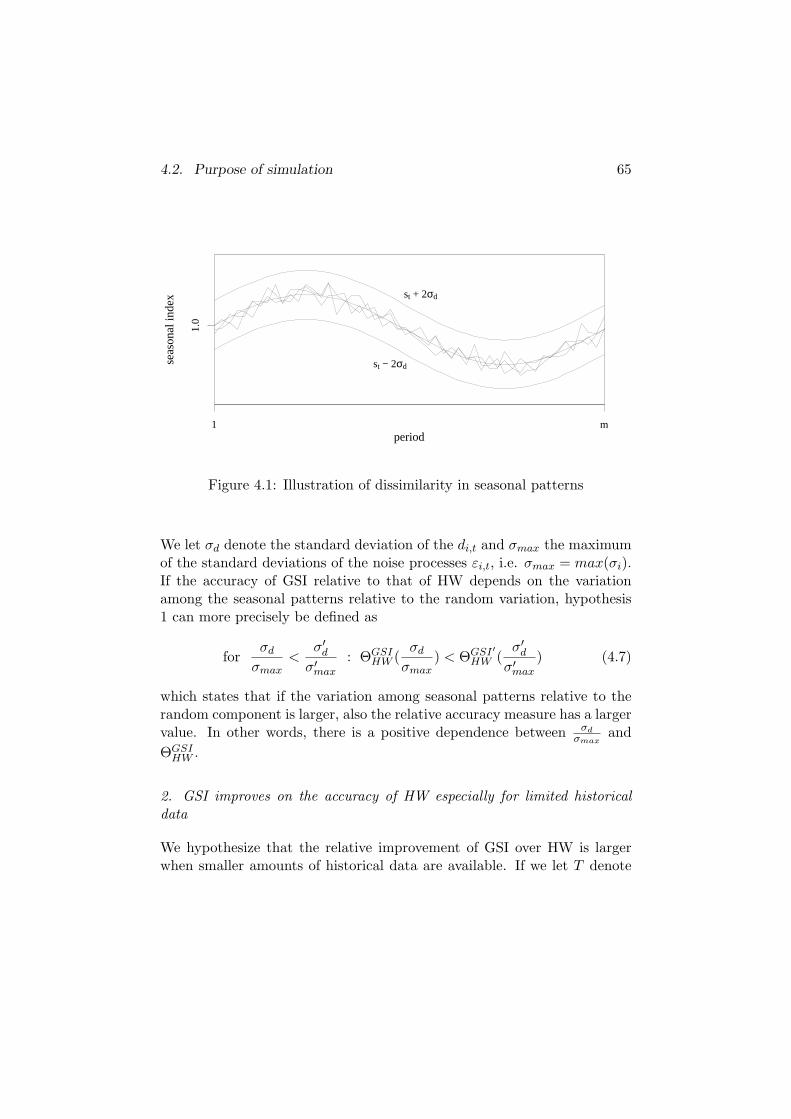
4.2. Purpose of simulation 65se
ason
al in
dex
period
st + 2σd
st − 2σd
1 m
1.0
Figure 4.1: Illustration of dissimilarity in seasonal patterns
We let σd denote the standard deviation of the di,t and σmax the maximumof the standard deviations of the noise processes εi,t, i.e. σmax = max(σi).If the accuracy of GSI relative to that of HW depends on the variationamong the seasonal patterns relative to the random variation, hypothesis1 can more precisely be defined as
forσd
σmax<
σ′d
σ′max
: ΘGSIHW (
σd
σmax) < ΘGSI′
HW (σ′
d
σ′max
) (4.7)
which states that if the variation among seasonal patterns relative to therandom component is larger, also the relative accuracy measure has a largervalue. In other words, there is a positive dependence between σd
σmaxand
ΘGSIHW .
2. GSI improves on the accuracy of HW especially for limited historicaldata
We hypothesize that the relative improvement of GSI over HW is largerwhen smaller amounts of historical data are available. If we let T denote

4.2. Purpose of simulation 66
the amount of historical data available, then this can be defined as
for T < T ′ : ΘGSIHW (T ) < ΘGSI′
HW (T ′) (4.8)
3. GSI is a robust method
We consider two definitions of robustness. Firstly, a method is robust ifit is not too much affected by departures from its assumptions. For GSI,this means that the accuracy ΘGSI should be insensitive to deviations fromthe underlying model. In particular, we consider the presence of differentseasonal patterns instead of identical patterns. Secondly, a robust methoddownweights the effect of extreme observations (Chatfield, 2000). GSI isthus more robust than HW if it is less sensitive to outliers. For this,we consider whether the accuracy measures of one method shows morevariation than that of the other method, in particular under large amountsof noise.
4. Negative correlations help GSI to improve on HW
Let ρ define the correlation between the random components of two series.Then this hypothesis says that GSI performs better for negative ρ comparedto positive ρ, and is specified by
for ρ < 0, ρ′ > 0 : ΘGSIHW (ρ) < ΘGSI′
HW (ρ′) (4.9)
Since it does not generate much insight to consider a full correlation matrix,we will look at groups of 2 time series and specify correlations to test thishypothesis.
5. The aggregation variant of GSI eliminates additional noise
In addition to the hypotheses from section 1.4.7, we examine one furtherhypothesis. In the simulations, the weights wi in GSI method are chosen tobe fixed and equal to σ−2
i∑Nj=1 σ−2
j
, as argued in Chapter 3. Other options have
disadvantages such as giving equal weight to all time series, or possibledivision by zero. This option gives lower weight to noisier time series.The approach with weights generalizes the method from Section 1.4, whichaggregates the time series to obtain better estimates, and this earliermethod is now a special case with weights equal to wi,t = li,t−1+bi,t−1∑N
j=1(lj,t−1+bj,t−1).
4.3. Parameter settings and data simulation 67
Since this GSI variant adds up the time series themselves, it may eliminateadditional noise such as that due to substitution effects. These are additiveeffects after all. We are thus interested in comparing the aggregation variantof the GSI method with the standard GSI method, by comparing datathat contains substitution effects and data that does not. The question iswhether
ΘGSI
(wi,t =
li,t−1 + bi,t−1∑Nj=1(lj,t−1 + bj,t−1)
)< ΘGSI
(wi =
σ−2i∑N
j=1 σ−2j
)(4.10)
4.3 Parameter settings and data simulation
The model developed in the previous chapter allows random simulationof data for which the GSI method is optimal. To investigate the aboveobjectives, data is simulated from a slightly modified model:
yi,t = (li,t−1 + bi,t−1)st−mvi,t (4.11a)li,t = (li,t−1 + bi,t−1)(1 + αi(vi,t − 1)) (4.11b)bi,t = bi,t−1 + (li,t−1 + bi,t−1)αiβi(vi,t − 1) (4.11c)
st = st−m + γst−m
N∑i=1
wi(vi,t − 1) + di,t (4.11d)
Firstly, this model replaces 1 + εi,t by vi,t. In model (3.22a)-(3.22d), thedisturbances are assumed to be normally distributed. Since errors aremultiplicative, this could result in negative time series values . Therefore,we use vi,t ∼ Γ(a, b) with a = 1/b and b = σ2
i , so that vi,t has meanab = 1 and variance ab2 = σ2
i . Although this reduces the probability ofyi,t becoming negative or problems due to division by zero, these can stilloccur if li,t + bi,t ≤ 0. If this happens, li,t + bi,t is truncated and set equalto a small number.
Secondly, this model introduces deviations from the common seasonalpattern, as discussed above. For di,t = 0, the equations of this model,when put in error-correction form, show equivalence with the GSI method(and with HW for N = 1). In order to generate simulated data, seed valuesli,0, bi,0 and s0, . . . , s−m+1 are specified, after which data from the modelis generated for t = 1, . . . , T .

4.3. Parameter settings and data simulation 68
In the simulations, data processes and types of forecasts are varied. Below,we discuss the corresponding model and forecast parameter settings. Allparameter settings are summarized in Tables 4.1 and 4.2. Many parametersare only scale parameters and thus their actual settings are not important.Their values relative to that of others are relevant. More precisely, theresults are determined by the amount of noise relative to the underlyingpattern. This determines the quality of the estimates and thus of theforecasts. For example, the value of the level li,t of a time series is notrelevant on its own, but the ratio between εi,t and li,t is. The same appliesfor the settings of other parameters and will be discussed below.
This allows for a reduction in the number of parameters to be considered,resulting in 1600 remaining combinations of parameter settings that areexamined. Some parameters are varied systematically on a grid of values.Other parameters are varied randomly on a continuous interval (parametersare randomly drawn from this interval). This is done if the numberof parameters that have to be specified is too large to vary them in asystematic way. For some parameters that are varied randomly, the intervalfrom which they are drawn is varied systematically.
Periodicity
We only consider twelve seasonal periods (m = 12), corresponding tomonthly time buckets. When there are more seasonal periods, e.g.,when m = 52 periods, GSI could have a potentially larger benefit, sinceestimation is then more difficult or more data is needed. Since this is thusmainly dependent on the amount of historical data (T ) and the amount ofnoise relative to m, we will take m fixed and vary T and the variance ofthe disturbances.
Length of historical data
We consider 4m and 6m periods of historical data. In each case a hold-outsample of 1 year is used. This means that 3m and 5m periods remain forestimation, i.e. obtaining estimates of smoothing parameters and initialstates. The estimation procedures are discussed in Section 4.4.
Group size
In order to get a wide range of clearly different group sizes, we take N ∈{2, 4, 8, 16, 32}.

4.3. Parameter settings and data simulation 69
Table 4.1: Parameters that remain fixed
Parameter Description Levelm Number of seasons 12l1,0 Initial level of first item 100cmax Maximum initial trend 0.008s{−m+1,...,0} Initial seasonal pattern SinusoidA Amplitude of seasonal pattern 0.2
Table 4.2: Levels at which parameters are varied
Parameter Description LevelTime seriesT Length of historical data 4m, 6mrmax 1, 4ri Ratio between li,0 and l1,0 ∈ [1, rmax]ci Ratio between bi,0 and li,0 ∈ [−cmax, cmax]αi ∈ [0, 1]βi ∈ [0, 1]γ ∈ [0, 1]wi Weights ∈ [0, 1]σ2
i Variance of noise ∈ [0, σ2max]
σmax 0.01, 0.03, 0.05, 0.07
Product groupsN Number of items in group 2, 4, 8, 16, 32σd Dissimilarity in 0, 0.01, 0.03, 0.05, 0.07
seasonal patterns
Forecastingh Forecast horizon 1, 4, 8, 12

4.3. Parameter settings and data simulation 70
Level and trend
The starting values of the time series are normalized by setting the levelof the first time series equal to li=1,t=0 = 100. The levels of the otherseries are set by specifying the ratio between the initial level li,0 of itemi and that of the first item: ri = li,0
l1,0. The ri are randomly drawn from
[1, rmax] and used to set li,0 = ril1,0. The ratios are used for initial valueswhen generating data. However, the levels evolve according to randomwalk processes, as well as due to trends. Especially under large amounts ofnoise or if trends move in opposite directions, the actual ratios may thusdeviate from the ri. For our regression analyses, we will therefore use anaverage ratio: r′i = (ri + li,T
l1,T)/2. Besides, to avoid using all the ri’s in a
regression, we will summarize the group by regressing on µr and σ2r , which
characterize the mean of r′i and its variation among the group of items.
The initial growth rate bi,0 is set by randomly drawing ci ∈ [−cmax, cmax]and setting bi,0 = cili,0, so that we end up with a initial trend between−cmax · m · 100% and cmax · m · 100% annually. Taking cmax = 0.008and m = 12, this gives an initial trend between approximately −10% and+10%. Only this value of cmax is considered since the performance of GSIdoes not depend on the trend, but on the amount of noise to which thetrend is subject. Since the trend development is incorporated in the level,the trends are not used in the regression. The parameters αi and βi aredrawn randomly from (0, 1). Once they are drawn, they are summarizedfor regression purposes by computing the proportion of each parametersin the intervals (0, 0.33), (0.33, 0.67) or (0.67, 1), denoted by α0.33
0 , α0.670.33,
α1.000.67, β0.33
0 , β0.670.33 and β1.00
0.67 .
Seasonal patterns
The model does not make an assumption on the shape of the seasonalpattern. In practice, however, the specific shape of this componentcan have an effect on the accuracy of the GSI method. The choice ofestimation procedure and the amount of noise relative to the seasonalpattern determine how difficult it is to estimate. Although the performanceof the GSI method can thus depend on type of pattern, we assume that itsinfluence is only minor. Therefore, we consider a single and fixed initialseasonal pattern {s−m+1, . . . , s0}, with sj−m = 1 + A · sin(2πj/m) forj = 1, . . . ,m and with A = 0.2. The smoothing parameter γ is drawnrandomly from (0, 1). The dissimilarity in seasonal patterns (see Section

4.3. Parameter settings and data simulation 71
4.2) is modeled via parameters di,t, which are drawn from N(0, σ2d). Thus,
σ2d determines the bandwidth within which all seasonal patterns of the
group lie and therefore the extent of dissimilarity. If σ2d = 0 the seasonal
patterns are identical.
Weights
For data that is simulated, w′i are drawn randomly from [0, 1] and then
normalized by taking wi = w′i∑N
i=1 w′i
, so that∑N
i=1 wi = 1. Taking weights
from one of the options mentioned under hypothesis 5 would mean that wewould influence the outcomes. In this way we ensure randomness of thedata. In the GSI method, weights wi are chosen to be fixed and equal to
σ−2i∑N
j=1 σ−2j
, as argued in Chapter 3.
Noise
The values of level, trend and seasonals themselves are not so important.Again, the amount of noise relative to the variation in underlying time seriescomponents is more relevant, or, in other words, the signal-to-noise ratio.We will thus choose noise variances (σ2
i ) based on the coefficient of variationof the time series. The coefficient of variation of deseasonalized anddetrended data, y′i,t = yi,t
(li,t−1+bi,t−1)st−m, is equal to cvi =
√V ar(vi,t)
E(vi,t)= σi
The noisiness of series is determined by the noise process in combinationwith parameters α, β and γ. These determine the signal-to-noise ratios forthe level, trend and seasonals. The value of cvi above gives informationon the volatility of the time series under perfect information about thetrend-seasonal cycle, but cvi in combination with parameters α, β and γdetermines the total variation in the series.
Forecast horizon
For all simulations, point forecasts will be made for h = 1, 4, 8 and 12 stepsahead.

4.4. Estimation 72
4.4 Estimation
Before we can make forecasts, we need estimates for initial values li,0,bi,0 and s−m+1, . . . , s0, and for parameters αi, βi, γ and wi. Thesecan be obtained by maximizing the conditional likelihood function or byminimizing some criterion that measures forecast errors such as the MSE.In Hyndman et al. (2002) several estimation methods were compared forfitting exponential smoothing state space models on data from the M3-competition, and minimizing the MSE was found on average to result inslightly more accurate forecasts than maximizing the likelihood. Althoughthese ways of obtaining estimates may be feasible approaches for simplermodels like the model underlying HW, the GSI model contains manyparameters, and thus finding optimal values in such a high dimensional(m + 1 + 5N dimensions) parameter space may be very time-consuming.
Instead of finding optimal estimates for all parameters and initial statesby a nonlinear optimization algorithm, we use a two-stage procedure andfirst obtain initial estimates of the states and then optimize the smoothingparameters. This is a common procedure for exponential smoothingmethods (and was used in our earlier experiments in Section 1.4). Thismeans that the smoothing parameters are optimized conditional on thevalues of the initial states. However, Makridakis and Hibon (1991) foundthat forecast accuracy is quite insensitive to initial values and the lossfunction used for fitting parameters. Although the exponential smoothingmethods under consideration were simpler than those studied here, weassume this conclusion to hold more generally if the run-in period is longenough before the forecast error is measured.
The two-step heuristic solution divides the historical data (T periods) intothree sections: an initialization period (I), an optimization period (O),and a hold-out sample (H), with T = I + O + H. Heuristic estimatesfor initial states are obtained using sample I, and a nonlinear optimizationalgorithm is used to find optimal parameter settings over sample O. We use2m periods for obtaining initial estimates and so 1m and 3m (for T = 4mand T = 6m respectively) periods remain for estimating the smoothingparameters.
Classical decomposition by ratio-to-moving-averages (RTMA) is used toobtain estimates for l0, b0 and s−m+1, . . . , s0. Assuming that a time series yt
consists of a trend component (TRt, including level), a seasonal component(St) and an irregular component (Et), the multiplicative decomposition

4.4. Estimation 73
model is yt = TCt · St · Et. The ratio-to-moving averages procedure thenconsists of the following steps:
1. Compute centered moving averages of order m through theinitialization period I to estimate the trend-cycle. Denote this byTCt, t = m/2 + 1, . . . , I −m/2.
2. Detrend the data by taking yt/TCt (which then corresponds to anestimate of St · Et), and average the estimates for each season toeliminate noise, so that we get m seasonal estimates. Normalizethese indices so they add to m, resulting in estimates s−m+1, . . . , s0
(corresponding to an estimate of St).
3. Deseasonalize the data using the above seasonal estimates(corresponding to an estimate of TCt ·Et) and compute a linear trendby fitting a simple regression line, in order to obtain l0 and b0.
For HW, we apply this procedure to each time series separately. ForGSI-AGG (GSI with aggregation of the time series, i.e. with weightswi,t = li,t−1+bi,t−1∑N
j=1(lj,t−1+bj,t−1)) we obtain seasonal estimates from the aggregate
time series and level and trend from each time series separately. Forthe general GSI method, however, we also need estimates of the wi. Inthe forecasting method, we will use weights equal to wi = σ−2
i∑Nj=1 σ−2
j
. To
estimate the σ2i , we fit a SSOE HW model to each time series separately,
by applying the corresponding HW method. Although this method isnot optimal if we assume the data follows the model underlying GSI, itstill gives reasonably good estimates of εi,t. These fitted errors can becalculated using the smoothed state estimates and the observation equation:εi,t = yi,t−(li,t−bi,t)st−m
(li,t−bi,t)st−m. This gives the following estimate for σ2
i :
σ2i =
∑Tt=1 ε 2
i,t
T − 3=
∑Tt=1
(yi,t−(li,t−1+bi,t−1)st−m
(li,t−1+bi,t−1)st−m
)2
T − 3(4.12)
Since we can only use sample I for fitting the HW model, T = I in this case.We use [T-number of smoothing parameters] in the divisor, as suggested byBowerman et al. (2005). Next, since the GSI model assumes the seasonalcomponent is common to all time series, we use the estimates of wi tofind initial estimates of the common seasonal pattern by computing sk =∑N
i=1 wisi,k for k = −m + 1, . . . , 0.

4.4. Estimation 74
After obtaining estimates for the initial states, each forecasting algorithmis run over I and O, so that the impact of poor initial estimates is offsetduring period I. The MSE is then calculated and minimized over periodO, by applying a nonlinear optimization algorithm. The same smoothingparameters are used throughout both I and O, but only measured overO. The starting values of the smoothing parameters are all taken tobe 0.5. Furthermore, they are constrained to 0 ≤ αi, βi, γ ≤ 1. Sincefor GSI and GSI-AGG all time series are interrelated via the commonseasonality equation, the sum of MSE’s is minimized, while for HW theMSE is optimized for each time series separately.
In summary, we have the following steps:
HW
1. Apply RTMA over I to obtain initial state estimates l0, b0 ands−m+1, . . . , s0
2. Make forecasts from t = 0 onwards. Measure MSE and optimize α,β and γ simultaneously over O.
GSI
1. (a) Fit a HW model for each item to obtain σ2i , and compute the
wi = σ−2i∑N
j=1 σ−2j
(b) Apply RTMA over I for each item separately to obtain seasonalestimates si,−m+1, . . . , si,0
(c) Compute the group seasonal indices as sk =∑N
i=1 wisi,k fork = −m + 1, . . . , 0
(d) Deseasonalize individual time series and run a linear regressionto obtain li,0 and bi,0
2. Make forecasts from t = 0 onwards. Measure MSE and optimize αi,βi and γ over O.

4.5. Evaluation and accuracy measurement 75
GSI-AGG
1. (a) Apply RTMA over I at the aggregate level to obtain seasonalestimates
(b) Deseasonalize individual time series and run a linear regressionto obtain li,0 and bi,0
2. Same as for GSI
We normalize the seasonal indices after each update of the estimates, asargued in Archibald and Koehler (2003). Although the model does notmake such an assumption on the seasonal indices, their interpretation wouldbe lost if they do no longer sum up to m. In that case, after successiveupdating, (li,t + bi,t)st−m could have a reasonable value, but, for example,with li,t−1 + bi,t−1 extremely large and st close to zero, or vice versa.
4.5 Evaluation and accuracy measurement
4.5.1 Evaluation
In general, an evaluation of forecasting methods by means of out-of-sample testing should preferably satisfy the characteristics of adequacyand diversity (Tashman, 2000). The former means that enough forecastsshould be made at each forecast horizon. Forecasts made from a singleorigin can be sensitive to occurrences specific to that forecast origin, soit should be adjusted to produce forecasts from multiple origins. Onlyif data were stationary this would not be a big concern (Fildes, 1992).By letting exponential smoothing algorithms run through the data andmaking forecasts from each consecutive origin, this problem is solved.But even with a rolling origin, the accuracy measures are sensitive tospecific phases of the available data. The latter characteristic thus refersto attaining cyclical diversity in order to avoid this sensitivity. If enoughdata is available, several sections should be used as hold-out sample. Usingmultiple time series also achieves this goal, as well as the former. Runninga simulation with many replications for different time series thus satisfiesboth requirements.
4.5. Evaluation and accuracy measurement 76
Number of replications
For each combination of parameter settings, multiple replications arecarried out. The number of replications per combination is determinedby statistical precision, based on confidence intervals. For example, forGSI, an approximate 95% confidence interval for µΘ = E(ΘGSI), based onk replications, is given by
ΘGSI(k)± tk−1,0.975
√S2(k)
k(4.13)
where ΘGSI(k) = 1k
∑kj=1 ΘGSI,j , with ΘGSI,j the accuracy of GSI on the
jth replication. The sample variance is given by S2(k) =∑k
j=1(ΘGSI,j −ΘGSI(k))2/k − 1. The number of replications that has to be made isdetermined by the following procedure, specified in Law and Kelton (1991).
If we let δ denote the relative error of ΘGSI(k), given by δ = |ΘGSI(k) −µΘ|/|µΘ|, then this error can be estimated by tk−1,0.975
√S2(k)
k /|ΘGSI(k)|.Replications are carried out until this quantity falls below δ. Then,|ΘGSI(k)| has a relative error of at most δ/(1 − δ) with a probabilityof approximately 0.95. We take δ = 0.09, so that δ/(1 − δ) ≈ 0.1.Since accuracy measures are computed for several forecasting methods, wecontinue making replications until all measures have a relative error of atmost δ.
Instead of generating a new time series for each replication, we only generatea new hold-out sample. In other words, the historical data remains thesame, but a new future sample path is simulated. In this way, we canreduce simulation time, since estimation only has to be done once. Toavoid the results being dependent on only a single set of historical data, werepeat this 50 times. For each case we continue replicating until the desiredprecision or the maximum number of iterations is reached. A minimum of10 replications is carried out, and a maximum of 200.
Table 4.3 presents some descriptive statistics for the simulations. Itshows i) the percentage of the cases were less than the maximum of 200replications were necessary to reach the desired precision of 0.95 for theconfidence intervals, ii) the average number of replications needed, and iii)the minimum precision attained if the maximum number of replicationswas reached. It is apparent that as the number of time series per group(N) increases, less replications are needed to attain a high precision. The

4.5. Evaluation and accuracy measurement 77
reason is that for larger groups, accuracy measures are averaged over moretime series, and are thus less sensitive to a few irregular time series.
Table 4.3: Descriptive statistics for simulations
N % cases < 200 repl. Av. nr. repl. Min. precision2 99.5 % 38.3 0.934 99.9 % 27.2 0.958 99.9 % 20.2 0.9116 100 % 16.3 0.9532 100 % 12.6 0.95
4.5.2 Accuracy measures
A suitable accuracy measure for comparing the forecasting methods in thisstudy should satisfy several requirements. Firstly, it should be adequatefrom a computational perspective. Secondly, it should be appropriate forour operational context. That is, we are interested in a loss function wherethe scale of each of the time series is important, and that is relevant tothe use of forecasts in operational decision making. We assume that it isused only for series that are not lumpy or intermittent. Thirdly, we wantto compare the accuracy of several methods across a number of time series,which means that forecast accuracy must be summarized over all theseseries.
From a computational perspective, we want a measure that is insensitiveto outliers, negative or (close to) zero values. For these reasons, manymeasures of accuracy for univariate forecasts are inadequate, since theymay be infinite, skewed or undefined, and can produce misleading results(Makridakis and Hibon, 1995; Hyndman and Koehler, 2005). Even themost common measures have drawbacks.
Scale-free measures based on percentage errors (et/yt · 100%) such as theMAPE are easy to interpret but have the disadvantage of being sensitiveto division by (close to) zero values of yt.
Measures based on relative errors (rt = et/eb,t, with eb,t the error of abenchmark method) are also sensitive to division by zero since eb,t can besmall. However, Armstrong and Collopy (1992) recommended the use of

4.5. Evaluation and accuracy measurement 78
relative absolute errors, |rt|, especially the geometric mean or median of|rt|, and also Fildes (1992) showed they have good properties.
Relative measures (such as RelMAD = MAD/MADb with MADb theMAD of a benchmark method) do not have these problems and have theadvantage of being interpretable. They require several forecasts on thesame series to enable a MAD to be computed, but this is not a problem inour study.
Scale-dependent measures such as MAD and MSE are suitable forcomparing different methods on the same set of data, but can not be usedto compare a single method on several data sets that have different scales.Besides, the MSE is sensitive to outliers.
In an operational context such as in inventory control and productionplanning, the size of the forecast errors determines the customer servicelevel. In this respect, the MSE is a relevant measure as a large error ismuch less desirable than two smaller ones whose sum is the same as thelarge error. The MSE is also used for determining safety stock levels, whichare set in order to provide a certain level of service to customers. Totalsafety stock investment depends on the standard deviation of forecast errorsand is equal to k
∑Ni=1 viσi, with k the safety factor, vi the unit value, and
σi the standard deviation of the forecast error over the replenishment leadtime.
The true value of this standard deviation is equal to√
true MSE and theRMSE calculated from the sample data is thus a reasonable estimate(Silver et al., 1998). Besides, the RMSE is at the same scale as thedata, and appropriate from a theoretical perspective (since the proceduresstudied minimize the MSE for their underlying models). However, MSEand RMSE are sensitive to outliers. The MAD is a substitute forRMSE that is less sensitive to outliers. For normally distributed errorsσ =
√π/2 (true MAD) ≈ 1.25 (true MAD) so that σ can be estimated by
1.25 MAD (Silver et al., 1998).
In order to summarize over all time series, we should decide whether wewant to give more weight to certain time series (such as fast moving items)or giving equal weight to all time series. Although the MAD is less affectedby outliers than the MSE (and is on the same scale as the data), both∑N
i=1 MAD and∑N
i=1 MSE are still strongly influenced by forecast errorsof fast moving items since it is scale dependent. Scale dependence can bea severe weakness in an error measure averaged across different series since

4.5. Evaluation and accuracy measurement 79
the unit of measurement in which a series is expressed can influence therelative rankings of different forecasting methods, which can be dominatedby a few series (Chatfield, 1988; Fildes, 1992).
Based on the above considerations, we opt for the use of the following twoaccuracy measures. Assume that historical data is available for periodst = 1, . . . , T , and that forecasts are made for t = T + j, j = 1, . . . ,H,with H the length of the hold-out sample. Based on an evaluation ofall common types of accuracy measures, Hyndman and Koehler (2005)advocates the use of scaled errors, where the error is scaled based on thein-sample MAD from a benchmark method. If we take the Naıve method(see e.g., Makridakis et al., 1998) as a benchmark, the scaled error is definedas
qi,t =yi,t − yi,t
1T−1
∑Tt=2 |yi,t − yi,t−1|
(4.14)
with yi,t the time series value and yi,t its forecast. The Mean AbsoluteScaled Error is then simply the mean of |qi,t|. In our case we take the meanover the hold-out sample and over all time series:
MASE =1N
N∑i=1
1H
T+H∑t=T+1
|qi,t| =1N
N∑i=1
MADi
MADb,i(4.15)
with MADi the MAD of time series i and MADb,i the MAD of thebenchmark method for time series i. Hyndman and Koehler (2005)recommends using the MASE for comparing accuracy across multiple timeseries, since it resolves all arithmetic issues mentioned above and is thussuitable for all situations. However, it does take away the scale of the data.Especially in our operational context, we would like to give more weightto certain time series. Therefore, we also suggest an alternative measure,based on
RelMADi =MADi
MADb,i(4.16)
with MADb,i the MAD of the out-of-sample Naıve method. To summarizeover all time series, we define the Relative Sum of MAD’s:
RelSMAD =∑N
i=1 MADi∑Ni=1 MADb,i
(4.17)
Another advantage of this measure is its interpretability. Both methods arecompared on the same sample, so that when RelMAD < 1, a method is

4.6. Experiments and results 80
more accurate than its benchmark. When RelMAD > 1, it is less accurate.The MASE does not have this interpretation for nonstationary time series.However, the RelSMAD assumes that all time series are on the same scale.Therefore, we will use these two measures simultaneously. Summarizing,these two measures satisfy the requirements with respect to the choice of theloss function, are appropriate from an operational context, and summarizeacross the time series.
4.6 Experiments and results
We are interested in comparing the accuracy of the GSI method with thatof the HW method. GSI generalizes HW and is intended to be used inthe same situations where HW is now used in practice. We determine theeffects of each of the parameters by first looking at the simulation resultsfor each of the parameters separately and then carrying out a regressionanalysis of the results. The simulations consist of the following steps:
1. Compare the accuracy of GSI and HW for various levels of each ofthe parameters.
2. Determine for which parameter settings the accuracy improvement ofGSI over HW is the largest.
3. Investigate how the accuracy and difference in accuracy depends onthe combination of parameter settings. This tells us which parametershave the largest influence on the results.
These results give a characterization of situations in which GSI is suitable,i.e. has an improvement over HW. Furthermore, they allow us to test thefirst three hypotheses. In order to test hypothesis 4 and 5, we conduct twomore experiments:
4. Investigate the influence of correlations on the accuracy of GSI
5. Compare the accuracy of GSI-AGG with that of GSI
Steps 1 and 2 are discussed in Section 4.6.1, while steps 3, 4 and 5 are dealtwith in Sections 4.6.2, 4.6.4 and 4.6.3, respectively.

4.6. Experiments and results 81
4.6.1 Accuracy improvement
We can now define the notation from Section 4.2 more explicitly. Theaccuracy ΘGSI and ΘHW is measured in terms of RelSMAD and MASE.We compare results on the relative improvement in accuracy of GSI overHW:
MASEGSIHW =
MASEGSI
MASEHW(4.18)
RelSMADGSIHW =
RelSMADGSI
RelSMADHW(4.19)
The parameters that are varied systematically are N , T , rmax, h, σd
and σmax. Below, we present a summary of the simulation results formeasures (4.18) and (4.19) for different parameter settings, averaged overall replications.
We removed one percent of the results with the lowest and highest values ofthe accuracy measures. The results contained some extreme values, causedby a few series that were extremely difficult to estimate due to the effects ofthe disturbance processes, and were not attributable to a specific parametercombination. By removing them, these values do not dominate the results.Furthermore, the aim of this study is to simulate realistic data satisfyingthe model, whereas not any set of data simulated from the model can beconsidered realistic or would occur in practice.
Below, we look at the effect on the results of each of the parameters N ,T , rmax, h, σd and σmax. The results are broken down with respect to thelevels of one or more of the parameters, and averaged over the levels of allother parameters.
First we look at some overall results, split up with respect to the extent ofdifference between the seasonal patterns in a group. Table 4.4 presents thevalues of MASEGSI
HW and RelSMADGSIHW for various levels of σd. It seems
that only if the seasonal patterns are identical (σd = 0), GSI improves onHW. If we split this out further with respect to the number of time seriesin a group, we see the same. However, we see that for small values ofσd, the improvement is more substantial for larger groups than for smallergroups. Table 4.5 shows this effect for low values of σd and various levels ofN . Improvements of up to 35% can be attained as the group size increase.However, these results are still averaged over several other parameters.

4.6. Experiments and results 82
An important parameter is the amount of noise in the time series. Thelevel of σmax determines the amount of noise present within the group oftime series. If we look at the results at various levels of this parameter (seeTable 4.6), we see that even when seasonal patterns are dissimilar therecan be accuracy improvement of GSI. However, a substantial amount ofnoise is needed for this. If seasonal patterns are nonidentical and there isonly little noise, HW has no difficulty forecasting at the item level. Only ifthere is substantial noise, is there an advantage of using a GSI approach. Itthus appears that the improvement becomes larger as the amount of noiseincreases.
Table 4.4: Relative accuracy of GSI compared to HW at various levels ofσd
σd MASEGSIHW RelSMADGSI
HW
0 0.82 0.850.01 1.11 1.130.03 1.34 1.350.05 1.42 1.440.07 1.48 1.50
Table 4.5: Relative accuracy of GSI compared to HW at various levels ofσd and N
σd N MASEGSIHW RelSMADGSI
HW
0 2 0.97 0.980 4 0.91 0.930 8 0.83 0.860 16 0.74 0.780 32 0.65 0.690.01 2 1.16 1.170.01 4 1.19 1.190.01 8 1.12 1.140.01 16 1.05 1.090.01 32 1.02 1.04
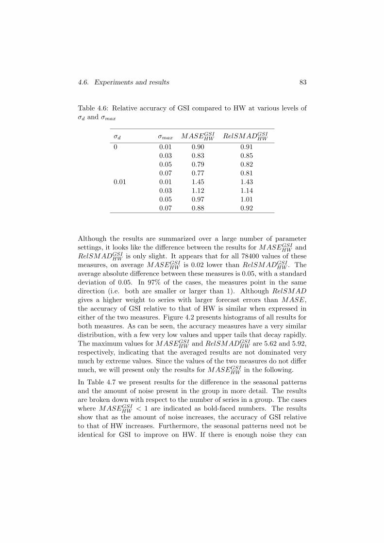
4.6. Experiments and results 83
Table 4.6: Relative accuracy of GSI compared to HW at various levels ofσd and σmax
σd σmax MASEGSIHW RelSMADGSI
HW
0 0.01 0.90 0.910.03 0.83 0.850.05 0.79 0.820.07 0.77 0.81
0.01 0.01 1.45 1.430.03 1.12 1.140.05 0.97 1.010.07 0.88 0.92
Although the results are summarized over a large number of parametersettings, it looks like the difference between the results for MASEGSI
HW andRelSMADGSI
HW is only slight. It appears that for all 78400 values of thesemeasures, on average MASEGSI
HW is 0.02 lower than RelSMADGSIHW . The
average absolute difference between these measures is 0.05, with a standarddeviation of 0.05. In 97% of the cases, the measures point in the samedirection (i.e. both are smaller or larger than 1). Although RelSMADgives a higher weight to series with larger forecast errors than MASE,the accuracy of GSI relative to that of HW is similar when expressed ineither of the two measures. Figure 4.2 presents histograms of all results forboth measures. As can be seen, the accuracy measures have a very similardistribution, with a few very low values and upper tails that decay rapidly.The maximum values for MASEGSI
HW and RelSMADGSIHW are 5.62 and 5.92,
respectively, indicating that the averaged results are not dominated verymuch by extreme values. Since the values of the two measures do not differmuch, we will present only the results for MASEGSI
HW in the following.
In Table 4.7 we present results for the difference in the seasonal patternsand the amount of noise present in the group in more detail. The resultsare broken down with respect to the number of series in a group. The caseswhere MASEGSI
HW < 1 are indicated as bold-faced numbers. The resultsshow that as the amount of noise increases, the accuracy of GSI relativeto that of HW increases. Furthermore, the seasonal patterns need not beidentical for GSI to improve on HW. If there is enough noise they can

4.6. Experiments and results 84
MASEHWGSI
rela
tive
freq
uenc
y
0 1 2 3 4 5 6 7 8 9
00.
020.
040.
060.
080.
1
RelSMADHWGSI
rela
tive
freq
uenc
y
0 1 2 3 4 5 6 7 8 90
0.02
0.04
0.06
0.08
0.1
Figure 4.2: Histograms of relative accuracy measures
be nonidentical to some extent. However, as the dissimilarity increases,the improvement diminishes. If the patterns become too dissimilar, HWperforms better in all cases.
Besides this, we see that the average improvement increases as the productgroups get larger. If the number of time series increases, the same amountof noise and dissimilarity gives larger improvements. The results for smallgroups are less pronounced since the results show more variability. Withsmall groups there is a larger chance of substantial differences in accuracyof both methods. For larger groups, the accuracy is averaged over moretime series and thus more stable. From Table 4.7, it appears that in caseof small product groups and little noise, it is more likely that HW appliedto each series separately results in better forecasts, while for large productgroups and substantial amounts of noise, GSI is more likely to performbetter.
In Table 4.8, we consider the effect of the forecast horizon on the accuracyimprovement. For σd = 0, the results confirm those from the empiricalstudy in Chapter 1. For a short forecast horizon, GSI clearly improveson HW. As the horizon increases, the advantage of GSI decreases, butremains. Surprisingly, for σd = 0 often the value of MASEGSI
HW increases as

4.6. Experiments and results 85
Table 4.7: Relative accuracy of GSI compared to HW at various levels ofN , σd and σmax (MASEGSI
HW )
σmax
N σd 0.01 0.03 0.05 0.072 0 0.99 0.99 0.91 0.992 0.01 1.33 1.18 1.10 1.042 0.03 1.46 1.31 1.26 1.132 0.05 1.47 1.35 1.28 1.182 0.07 1.44 1.35 1.33 1.334 0 0.94 0.94 0.89 0.884 0.01 1.43 1.21 1.10 1.004 0.03 1.61 1.38 1.29 1.224 0.05 1.65 1.41 1.38 1.274 0.07 1.62 1.52 1.38 1.368 0 0.89 0.83 0.84 0.788 0.01 1.48 1.11 0.99 0.898 0.03 1.69 1.42 1.29 1.138 0.05 1.79 1.51 1.31 1.298 0.07 1.78 1.61 1.45 1.3216 0 0.86 0.74 0.67 0.6816 0.01 1.47 1.06 0.86 0.7716 0.03 1.78 1.48 1.20 1.0216 0.05 1.83 1.50 1.31 1.1816 0.07 1.88 1.59 1.40 1.1632 0 0.82 0.64 0.61 0.5232 0.01 1.54 1.02 0.82 0.6932 0.03 1.82 1.32 1.06 0.9132 0.05 1.90 1.56 1.24 1.0132 0.07 1.93 1.60 1.35 1.19

4.6. Experiments and results 86
the forecast horizon increases, while for σd > 0 it decreases as h increases.This effect is present for all values of N and also for RelSMADGSI
HW .
Table 4.8: Relative accuracy of GSI compared to HW (MASEGSIHW ) for
N = 32 at various levels of σd, h and σmax
σmax
N σd h 0.01 0.03 0.05 0.0732 0 1 0.76 0.55 0.49 0.4332 0 4 0.76 0.61 0.61 0.4932 0 8 0.84 0.65 0.63 0.5632 0 12 0.91 0.75 0.71 0.6032 0.1 1 1.87 1.16 0.85 0.7632 0.1 4 1.47 1.01 0.73 0.6632 0.1 8 1.48 0.96 0.87 0.6432 0.1 12 1.35 0.96 0.82 0.71
Next, we consider the effect of the amount of historical data available formaking forecasts. In Table 4.9 we compare a setting with T = 48 witha setting with T = 72. The bold-faced results now indicate whether theMASEGSI
HW is lower for T = 48 or for T = 72.
If we look at all results, including the cases where GSI is less accuratethan HW, we can clearly see the effect of using more historical data. Onaverage, with less historical data, GSI compares favorably with HW (thereis a larger number of bold-faced results). At a more detailed level, we haveseen (Table 4.7) that the largest performance improvements are reachedwhen there are many products in combination with a lot of noise. If weconsider these cases in Table 4.9, it appears that additional data may helpas well to improve the accuracy of GSI, while for small groups, there isnot a large difference between the results for T = 48 and T = 72. It isdifficult to give an explanation for this difference, since both GSI and HWmay benefit from additional data.
Theoretically, the homogeneity of the series within a group theoreticallyshould not have an impact on the results. Seasonality is assumed to bemultiplicative and the error processes are relative, meaning that the scaleof the time series is not relevant. However, in almost all cases, MASEGSI
HW
is smaller for rmax = maxi(li,0/l1,0) = 1 than for rmax = 4.

4.6. Experiments and results 87
Table 4.9: Relative accuracy of GSI compared to HW (MASEGSIHW ) at
various levels of N , σd, T and σmax
T = 48 T = 72σmax σmax
N σd 0.01 0.03 0.05 0.07 0.01 0.03 0.05 0.072 0 0.98 0.99 0.97 0.98 1.00 1.00 0.86 0.992 0.01 1.21 1.12 1.07 1.04 1.44 1.25 1.12 1.052 0.03 1.32 1.25 1.18 1.12 1.61 1.38 1.33 1.132 0.05 1.33 1.28 1.22 1.13 1.61 1.42 1.34 1.222 0.07 1.34 1.28 1.28 1.24 1.55 1.42 1.38 1.414 0 0.92 0.92 0.91 0.87 0.97 0.95 0.87 0.894 0.01 1.31 1.10 1.03 0.98 1.55 1.31 1.18 1.014 0.03 1.42 1.30 1.19 1.14 1.80 1.47 1.40 1.314 0.05 1.46 1.33 1.25 1.22 1.84 1.48 1.50 1.324 0.07 1.45 1.41 1.32 1.25 1.79 1.64 1.44 1.478 0 0.88 0.88 0.85 0.87 0.90 0.78 0.82 0.708 0.01 1.35 1.07 0.97 0.93 1.61 1.15 1.01 0.848 0.03 1.50 1.35 1.24 1.13 1.89 1.49 1.35 1.138 0.05 1.58 1.44 1.27 1.21 1.99 1.58 1.36 1.378 0.07 1.59 1.47 1.34 1.22 1.97 1.76 1.57 1.4116 0 0.86 0.82 0.75 0.76 0.87 0.66 0.60 0.6116 0.01 1.37 1.08 0.88 0.86 1.58 1.04 0.84 0.6916 0.03 1.56 1.33 1.23 1.10 2.00 1.64 1.17 0.9416 0.05 1.62 1.44 1.31 1.15 2.05 1.55 1.31 1.2016 0.07 1.67 1.49 1.35 1.18 2.09 1.68 1.45 1.1532 0 0.85 0.79 0.71 0.63 0.79 0.49 0.51 0.4132 0.01 1.40 1.06 0.89 0.76 1.69 0.98 0.75 0.6232 0.03 1.63 1.36 1.19 0.98 2.01 1.27 0.94 0.8432 0.05 1.69 1.48 1.32 1.11 2.11 1.63 1.15 0.9132 0.07 1.72 1.53 1.40 1.22 2.15 1.67 1.30 1.16

4.6. Experiments and results 88
Table 4.10: Relative accuracy of GSI compared to HW (MASEGSIHW ) at
various levels of rmax, N , and σmax
σmax
rmax N 0.01 0.03 0.05 0.071 2 1.29 1.21 1.16 1.111 4 1.40 1.26 1.20 1.141 8 1.47 1.26 1.16 1.071 16 1.51 1.24 1.09 0.941 32 1.55 1.21 1.01 0.85
4 2 1.39 1.26 1.19 1.164 4 1.51 1.33 1.22 1.154 8 1.58 1.33 1.20 1.094 16 1.62 1.31 1.09 0.994 32 1.66 1.24 1.02 0.88
Table 4.10 compares these two settings, were the lowest values of MASEGSIHW
are bold-faced. Although the value of rmax does not matter theoretically,it supports the conclusions from research on hierarchical forecasting.The literature reviewed in Chapter 2 suggested that groups should behomogeneous for hierarchical approaches to improve accuracy of directforecasting approaches.
From the above results, it seems that the level of σd (the difference in theseasonal patterns) relative to that of σmax (the maximum amount of noisein the group) has a significant impact on the results. In Table 4.11 theresults for all values of σd/σmax and N are shown, and in Figure 4.3 theresults for log(σd/σmax) are plotted. Both show a clear relationship betweenMASEGSI
HW and the value of σd/σmax. The lower the value of σd/σmax, thelarger the accuracy improvement, in particular for larger values of N .
Summarizing, we have seen that GSI gives more accurate forecasts than HWin many situations, and that, on average, larger accuracy improvements ofGSI over HW can be achieved for:
- similar seasonal patterns (small value of σd), or less similar patternsif there is substantial noise (a larger value of σmax)
- larger amounts of noise (larger σmax)

4.6. Experiments and results 89
Table 4.11: Relative accuracy of GSI compared to HW (MASEGSIHW ) at
various levels of σd/σmax and N
Nσd/σmax 2 4 8 16 320 0.97 0.91 0.83 0.74 0.650.14 1.04 1.00 0.89 0.77 0.690.20 1.10 1.10 0.99 0.86 0.820.33 1.18 1.21 1.11 1.06 0.960.43 1.13 1.22 1.13 1.02 0.910.60 1.26 1.29 1.29 1.20 1.060.71 1.18 1.27 1.29 1.18 1.011 1.31 1.39 1.38 1.36 1.321.40 1.33 1.38 1.45 1.40 1.351.67 1.35 1.41 1.51 1.50 1.562.33 1.35 1.52 1.61 1.59 1.603 1.46 1.61 1.69 1.78 1.825 1.47 1.65 1.79 1.83 1.907 1.44 1.62 1.78 1.88 1.93
- larger groups (larger N)- short to medium forecast horizons (small h)- less historical data (small T )- less variability among the levels of the time series in a group (small
rmax)
In the next section, we investigate the above relationships more formallyand determine which of the parameters have the strongest effects on theresults. By using an analysis of variance and a regression analysis, we canconsider all parameters together.
4.6.2 Impact of parameters on accuracy improvement
We first determine which of the parameters have the strongest impacton the accuracy improvement. We do this by using the analysis ofvariance procedure (ANOVA). This analysis tells us if distinct levels of eachof the parameters result in significantly different values of the accuracy
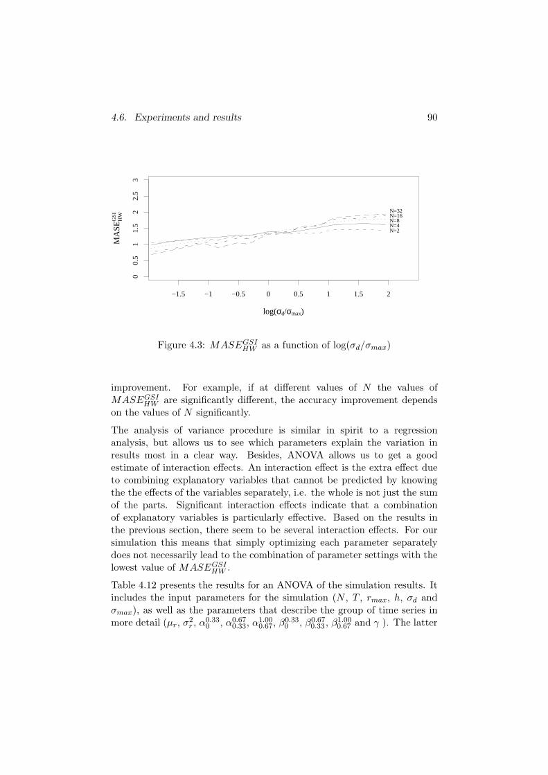
4.6. Experiments and results 90
log(σd/σmax)
MA
SEH
WG
SI
N=2N=4N=8N=16N=32
−1.5 −1 −0.5 0 0.5 1 1.5 2
00.
51
1.5
22.
53
Figure 4.3: MASEGSIHW as a function of log(σd/σmax)
improvement. For example, if at different values of N the values ofMASEGSI
HW are significantly different, the accuracy improvement dependson the values of N significantly.
The analysis of variance procedure is similar in spirit to a regressionanalysis, but allows us to see which parameters explain the variation inresults most in a clear way. Besides, ANOVA allows us to get a goodestimate of interaction effects. An interaction effect is the extra effect dueto combining explanatory variables that cannot be predicted by knowingthe the effects of the variables separately, i.e. the whole is not just the sumof the parts. Significant interaction effects indicate that a combinationof explanatory variables is particularly effective. Based on the results inthe previous section, there seem to be several interaction effects. For oursimulation this means that simply optimizing each parameter separatelydoes not necessarily lead to the combination of parameter settings with thelowest value of MASEGSI
HW .
Table 4.12 presents the results for an ANOVA of the simulation results. Itincludes the input parameters for the simulation (N , T , rmax, h, σd andσmax), as well as the parameters that describe the group of time series inmore detail (µr, σ2
r , α0.330 , α0.67
0.33, α1.000.67, β0.33
0 , β0.670.33 , β1.00
0.67 and γ ). The latter

4.6. Experiments and results 91
were calculated from the set of time series that were simulated using theinput parameters. In addition, we included the most important interactioneffects, i.e. those interaction effects that were both significant and werelarger than 50.
Firstly, it appears that N and T show large values of their respective sumof squares (SS). This is not surprising, since they take on larger values thanthe other parameters. If we take into account the relative magnitudes ofthe parameters, in particular the SS values of σd and σmax are large. Thiscorresponds to the findings in the previous section, where these parameterswere found to be important determinants of accuracy improvement. TheSS value of h on the other hand is relatively small, indicating that benefitsof GSI do not apply to only a particular forecast horizon.
Secondly, let us consider the set of parameters that were determined fromthe simulated data. In Table 4.12, the parameter β1.00
0.67 are omitted. Thereason is that at least one of the variables α0.33
0 , α0.670.33, α1.00
0.67, β0.330 , β0.67
0.33
or β1.000.67 has to be removed from the analysis to avoid singularities (since
both α0.330 + α0.67
0.33 + α1.000.67 = 1 and β0.33
0 + β0.670.33 + β1.00
0.67 = 1). The valuesof β0.33
0 , β0.670.33 or β1.00
0.67 are much lower than those of α0.330 , α0.67
0.33 and α1.000.67,
but would be comparable if for example α1.000.67 was omitted instead of β1.00
0.67 .In either case, it appears that if a group has a larger portion of time serieswith high αi’s or βi’s, the accuracy improvement show more variability.Since also rmax has a high SS value, this shows that groups of time serieswith more heterogeneous demand patterns show more variation in accuracyimprovement. This is not surprising, since more in those cases, the timeseries are more variable, and thus more difficult to forecasts.
For most of the parameters the effects on the results are clearly significant,with very large F-values. However, three parameters do not have asignificant effect on the accuracy improvement: µr, σ2
r and γ. In contrastwith the values of the αi’s or βi’s, the value of γ appears to have no clearinfluence on the accuracy improvement.
Thirdly, we look at the interaction effects. Here, the results conform to whatwe have seen in the previous section. Especially the values of σd and σmax incombination with several other parameters can yield an additional accuracyimprovement. Especially combination including the input parameters N ,T and h appear to explain a significant part of the variation in MASEGSI
HW .
Now we know which parameters explain most of the variance in the accuracyimprovement, let us be more precise about the impact of certain parameters.
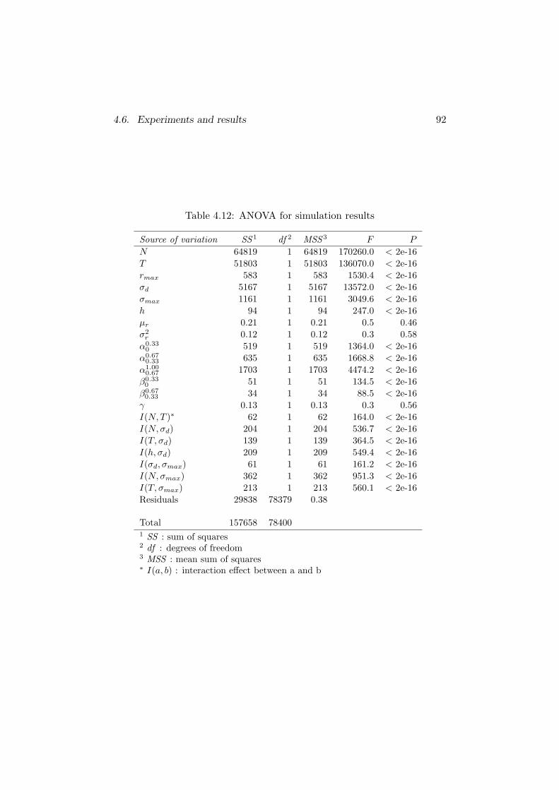
4.6. Experiments and results 92
Table 4.12: ANOVA for simulation results
Source of variation SS 1 df 2 MSS 3 F P
N 64819 1 64819 170260.0 < 2e-16T 51803 1 51803 136070.0 < 2e-16rmax 583 1 583 1530.4 < 2e-16σd 5167 1 5167 13572.0 < 2e-16σmax 1161 1 1161 3049.6 < 2e-16h 94 1 94 247.0 < 2e-16µr 0.21 1 0.21 0.5 0.46σ2
r 0.12 1 0.12 0.3 0.58α0.33
0 519 1 519 1364.0 < 2e-16α0.67
0.33 635 1 635 1668.8 < 2e-16α1.00
0.67 1703 1 1703 4474.2 < 2e-16β0.33
0 51 1 51 134.5 < 2e-16β0.67
0.33 34 1 34 88.5 < 2e-16γ 0.13 1 0.13 0.3 0.56I(N,T )∗ 62 1 62 164.0 < 2e-16I(N,σd) 204 1 204 536.7 < 2e-16I(T, σd) 139 1 139 364.5 < 2e-16I(h, σd) 209 1 209 549.4 < 2e-16I(σd, σmax) 61 1 61 161.2 < 2e-16I(N,σmax) 362 1 362 951.3 < 2e-16I(T, σmax) 213 1 213 560.1 < 2e-16Residuals 29838 78379 0.38
Total 157658 784001 SS : sum of squares2 df : degrees of freedom3 MSS : mean sum of squares∗ I(a, b) : interaction effect between a and b
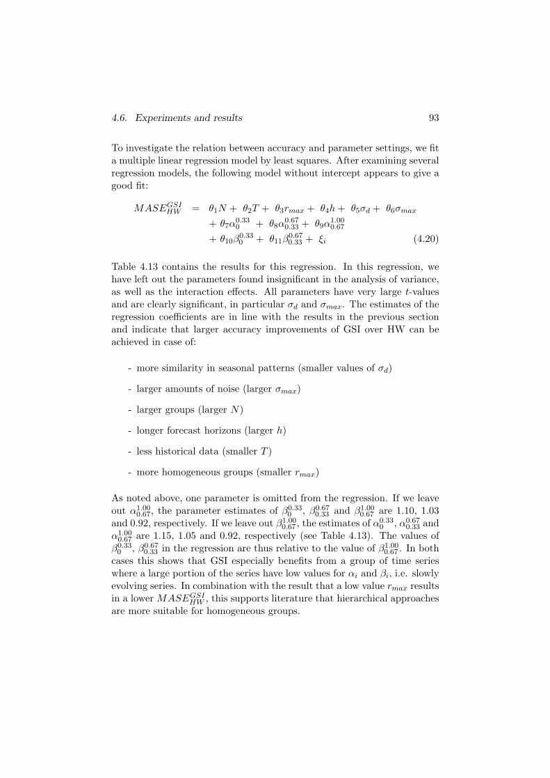
4.6. Experiments and results 93
To investigate the relation between accuracy and parameter settings, we fita multiple linear regression model by least squares. After examining severalregression models, the following model without intercept appears to give agood fit:
MASEGSIHW = θ1N + θ2T + θ3rmax + θ4h + θ5σd + θ6σmax
+ θ7α0.330 + θ8α
0.670.33 + θ9α
1.000.67
+ θ10β0.330 + θ11β
0.670.33 + ξi (4.20)
Table 4.13 contains the results for this regression. In this regression, wehave left out the parameters found insignificant in the analysis of variance,as well as the interaction effects. All parameters have very large t-valuesand are clearly significant, in particular σd and σmax. The estimates of theregression coefficients are in line with the results in the previous sectionand indicate that larger accuracy improvements of GSI over HW can beachieved in case of:
- more similarity in seasonal patterns (smaller values of σd)
- larger amounts of noise (larger σmax)
- larger groups (larger N)
- longer forecast horizons (larger h)
- less historical data (smaller T )
- more homogeneous groups (smaller rmax)
As noted above, one parameter is omitted from the regression. If we leaveout α1.00
0.67, the parameter estimates of β0.330 , β0.67
0.33 and β1.000.67 are 1.10, 1.03
and 0.92, respectively. If we leave out β1.000.67 , the estimates of α0.33
0 , α0.670.33 and
α1.000.67 are 1.15, 1.05 and 0.92, respectively (see Table 4.13). The values of
β0.330 , β0.67
0.33 in the regression are thus relative to the value of β1.000.67 . In both
cases this shows that GSI especially benefits from a group of time serieswhere a large portion of the series have low values for αi and βi, i.e. slowlyevolving series. In combination with the result that a low value rmax resultsin a lower MASEGSI
HW , this supports literature that hierarchical approachesare more suitable for homogeneous groups.

4.6. Experiments and results 94
In this section, we discussed the results for MASEGSIHW . The results for
RelSMADGSIHW are largely comparable and lead to the same conclusions.
They can be found in Tables 1 and 2 in the appendix.
Table 4.13: Results for regression of MASEGSIHW on parameters (eq. 4.20)
Parameter Coefficient t P
N -0.0024 -11.6 < 2e-16T 0.0037 19.9 < 2e-16rmax 0.0183 12.2 < 2e-16σd 8.6863 98.9 < 2e-16σmax -7.5374 -75.0 < 2e-16h -0.0192 -35.4 < 2e-16α0.33
0 1.1515 67.7 < 2e-16α0.67
0.33 1.0467 61.0 < 2e-16α1.00
0.67 0.9175 54.0 < 2e-16β0.33
0 0.1802 14.5 < 2e-16β0.67
0.33 0.1141 9.2 < 2e-16
R2 = 0.81F -statistic = 29010, P -value = < 2.2e-16
4.6.3 Comparison between GSI and GSI-AGG
Next, we compare the relative performance of GSI with GSI-AGG, thevariant of GSI that aggregates the time series to estimate the joint seasonalpattern. for this comparison, let
MASEAGGHW =
MASEAGG
MASEHW(4.21)
RelSMADAGGHW =
RelSMADAGG
RelSMADHW(4.22)
Compared to the results for GSI, the results for the accuracy improvementare now more skewed. There are some large values that dominate the resultsfor GSI-AGG when averaged over all replications. Compared to Figure 4.2,the histograms in Figure 4.4 clearly show heavier tails in the distributionof results. For MASEGSI
HW and RelSMADGSIHW the maximum values were

4.6. Experiments and results 95
5.62 and 5.92, respectively, while for MASEAGGHW and RelSMADAGG
HW theywere 88.23 and 90.83, respectively.
MASEHWAGG
rela
tive
freq
uenc
y
0 1 2 3 4 5 6 7 8 9
00.
020.
040.
060.
080.
1
RelSMADHWAGG
rela
tive
freq
uenc
y
0 1 2 3 4 5 6 7 8 9
00.
020.
040.
060.
080.
1
Figure 4.4: Histograms of relative accuracy measures
The main difference between GSI-AGG and GSI is that the weights wi aretime-dependent (i.e. wi,t). Since the forecasting procedure now followschanges in the time series more closely, this also introduces more volatilityin the forecasts. This is confirmed by the simulation results, for which ananalysis of variance of MASEAGG
HW is presented in Table 4.15. We only listthe main effects, and do not report interaction effects. We found at least29 interaction effects that are significant at the 95% confidence level. Thisindicates that many of the results are determined by specific combinationsof parameter settings.
For GSI-AGG the same parameters as for GSI explain the variability inaccuracy improvement. Again N , T , σd and σmax, have a large effect onMASEAGG
HW . Also h has a large effect now. However, in this case, rmax
is insignificant. This is in line with theory, since the value of rmax is notimportant theoretically. The seasonal pattern is multiplicative and the levelof the time series should not matter for estimation. In case of GSI this wasnot the case, but for GSI-AGG, which aggregates data explicitly, the scaleof the time series indeed does not matter.

4.6. Experiments and results 96
A regression analysis shows a similar picture. We compared severalregression models and found a maximum explanatory value equal to R2 =0.44 (as opposed to 0.81 for GSI), indicating that the parameters can onlypartly explain the changes in the accuracy improvement. Altogether, thevariability in results makes it difficult to predict in which situations GSI-AGG improves on HW. In Section 4.7, we present some further results onthe robustness of both the GSI and GSI-AGG methods, which show thatGSI is more robust than GSI-AGG.
As in the previous section, the results for RelSMADAGGHW were largely the
same as for MASEAGGHW , and are thus not reported here.
Table 4.14: ANOVA for simulation results
Source of variation SS 1 df 2 MSS 3 F P
N 1108055 1 1108055 24506.3 < 2e-16T 25638 1 25638 567.0 < 2e-16rmax 70 1 70 1.5 0.21σd 10799 1 10799 238.8 < 2e-16σmax 80946 1 80946 1790.2 < 2e-16h 92770 1 92770 2051.7 < 2e-16µr 44 1 44 1.0 0.32σ2
r 3 1 3 0.1 0.80α0.33
0 8841 1 8841 195.5 < 2e-16α0.67
0.33 9588 1 9588 212.0 < 2e-16α1.00
0.67 43539 1 43539 962.9 < 2e-16β0.33
0 896 1 896 19.8 9e-06β0.67
0.33 87 1 87 1.9 0.17γ 63 1 63 1.4 0.24Residuals 3544236 78386 45
Total 4925575 784001 SS : sum of squares2 df : degrees of freedom3 MSS : mean sum of squares
4.6. Experiments and results 97
4.6.4 Effect of correlation on accuracy improvement
In the above, we have assumed that the time series were uncorrelated.However, in practice, groups of products from the same product categoryare likely to have correlated demand patterns. In this section we discusssimulation experiments where the disturbance terms are correlated acrosstime series. We do this for groups of size N = 2. For larger groups oftime series, we would have to construct large covariance matrices in orderto draw disturbances from a multivariate distribution. Apart from beingdifficult due to restrictions on covariance matrices, complex matrices donot give much insight into the effect of cross-correlations.
In the above simulations, we generated data from model (4.11a)-(4.11d),where the disturbances were Gamma distributed. Here, we are interestedin generating vi,t ∼ Γ(ai, bi) for i = 1, 2 and t = 1, . . . , T , with v1,t andv2,t correlated with Cor(v1, v2) = ρ. A difficulty is that not all values ofρ between -1 and +1 are theoretically consistent with a set of ai’s, placingrestrictions on ρ (Schmeiser and Lal, 1982). To work around this problem,we will return to normal errors, and truncate them if necessary. We generatedata for groups of two series, having a correlation of -0.9, -0.6, -0.3, 0, 0.3,0.6 and 0.9.
Table 4.15 shows summaries of an analysis of variance for both MASEGSIHW
and MASEAGGHW . For MASEGSI
HW , the effect of correlation is not very large,but significant. For MASEAGG
HW , the effect is clearly insignificant. If wecarry out a regression on the significant parameters of MASEGSI
HW , we find(see Table 4.16) that correlation has a negative impact on the accuracyimprovement, indicating that only positive correlations yield a lower valueof the relative accuracy measure and negative correlations result in a highervalue.
The detailed results are not presented here, but show that in some cases,when correlation is very high (0.9) or very low (-0.9), there is someclear improvement over HW. But statistically, the effect of the correlationcoefficient is only small or insignificant. A possible explanation is the groupsize considered for this experiment. In the simulation results withoutcorrelation, we have seen that especially for larger groups, significantaccuracy improvements can be achieved. But as mentioned, it is morecomplex to investigate this in a systematic and informative way.

4.7. Test of hypotheses 98
Table 4.15: ANOVA for simulation results with correlation
MASEGSIHW MASEAGG
HW
Source of variation SS 1 P SS 1 P dfρ 11 1e-05 1 0.23 1T 70488 < 2e-16 88913 < 2e-16 1rmax 221 < 2e-16 373 < 2e-16 1σd 1148 < 2e-16 2144 < 2e-16 1σmax 6 9.7e-04 1053 < 2e-16 1h 135 < 2e-16 310 < 2e-16 1µr 2 0.08 1 0.14 1σ2
r 0.03 0.81 1 0.26 1α0.33
0 21 1.7e-09 1068 < 2e-16 1α0.67
0.33 99 < 2e-16 440 < 2e-16 1α1.00
0.67 792 < 2e-16 1371 < 2e-16 1β0.33
0 4 0.01 404 < 2e-16 1β0.67
0.33 1 0.17 46 < 2e-16 1γ 1 0.27 3 0.02 1Residuals 25745 25022 43890
Total 98674 121150 439041 SS : sum of squares2 df : degrees of freedom
4.7 Test of hypotheses
Most of the hypothesis were already discussed above in the presentation ofthe results. Below we briefly discuss all hypotheses.
1. The improvement of GSI over HW depends on the variation among theseasonal patterns relative to the random variation
There is a clear relationship between the similarity in seasonal patternsand the random variation. In Figure 4.3 a linear relationship is shownbetween the log of the ratio of these two source of variation and theaccuracy improvement. If the variation among the seasonal patterns islow compared to the random variation, GSI improves on HW. Furthermore,from the simulation results we see that seasonal patterns need not be strictly

4.7. Test of hypotheses 99
Table 4.16: Results for regression of MASEGSIHW on parameters with
correlation
Parameter Coefficient t P
ρ -0.0268 -4.4 1.1 e-05T 0.0074 24.2 2.5 e-128rmax 0.0139 5.7 1.1 e-08σd 5.1312 35.9 < 2e-16σmax -2.2725 -13.9 7.5 e-44h -0.0217 -24.6 1.5 e-132α0.33
0 0.8504 36.3 2.5 e-284α0.67
0.33 0.8675 37.2 1.4 e-298α1.00
0.67 0.8360 35.9 1.3 e-277β0.33
0 0.0273 2.5 1.3 e-02
R2 = 0.74F -statistic = 12430, P -value = < 2.2e-16
identical. Dissimilar patterns are allowed as long as there is sufficientrandom variation compared to the variation among the patterns.
2. GSI improves on the accuracy of HW especially for limited historicaldata
A detailed examination of the results showed this is not universally true,and that it depends on the value of other parameters. The regression resultsin Table 4.13, however, show a significant and positive value of T , meaningthat the hypothesis is correct. If the amount of historical data T is smaller,the accuracy improvement is larger on average.
3. GSI is a robust method
Firstly, we have seen that GSI can improve on HW even if the seasonalpatterns are not identical. This shows that the method is robust todeviations from one of its major assumptions. Secondly, GSI can beconsidered to be more robust than HW if it is less sensitive to outliers.In Table 4.17, we present the mean and standard deviation of MASE andRelSMAD for both GSI, GSI-AGG and HW. These values are calculated

4.7. Test of hypotheses 100
over all parameter combinations. Clearly, the mean and standard deviationof GSI are lower than those of GSI-AGG and HW. In Table 4.18, the valuesare split up with respect to the amount of noise (σmax). As the amount ofnoise increases, the chance of outliers occurring also increases. Especiallyfor HW, for larger amounts of noise, the mean and standard deviation goup significantly. GSI is thus more robust than GSI-AGG and HW since theaccuracy measures are lower and show less variation for GSI than for theother methods, in particular under large amounts of noise.
Table 4.17: Robustness results for GSI and HW
MASE RelSMAD
Method Mean St.dev. Mean St.dev.GSI 1.44 1.06 1.06 0.94GSI-AGG 2.94 5.32 2.17 4.03HW 20.55 170.70 7.29 52.41
4. Negative correlations help GSI to improve on HW
Earlier studies on GSI-AGG and hierarchical forecasting argue thataggregation approaches work under cross correlations among demandpatterns. However, from Section 4.6.4 it appears that the effect ofcorrelation is only very small. Furthermore, negative correlation resultsin a higher value of the relative accuracy MASEGSI
HW instead of a lowervalue. As mentioned above, the small group size may cause the effects tobe less pronounced.
5. The aggregation variant of GSI eliminates additional noise
Based on the earlier studies, we would expect that especially GSI-AGGbenefits from correlated time series, since it aggregates the data. In this wayrandom variations such as substitution effects would cancel out. However,for GSI-AGG, correlation does not significantly affect the relative accuracy,as measured by MASEAGG
HW .

4.8. Classical HW versus SSOE variant 101
Table 4.18: Robustness results for GSI and HW
MASE RelSMAD
Method σmax Mean St.dev. Mean St.dev.GSI 0.01 1.00 0.62 0.60 0.32
0.03 1.35 0.90 0.93 0.720.05 1.60 1.12 1.23 1.000.07 1.80 1.29 1.47 1.23
GSI-AGG 0.01 2.99 5.62 2.01 4.160.03 2.89 5.23 2.08 4.020.05 2.91 5.24 2.20 3.910.07 2.96 5.18 2.39 4.00
HW 0.01 2.49 55.14 0.85 13.550.03 16.11 154.89 5.45 44.120.05 25.91 192.83 8.79 56.390.07 37.43 226.54 13.95 74.43
4.8 Classical HW versus SSOE variant
In Section 3.3.2, we discussed the SSOE model underlying Holt-Winters.Compared to the classical HW procedure, the optimal method resultingfrom this model is slightly different. The classical HW procedure containslt in the updating equation for seasonality, whereas the method resultingfrom the SSOE model contains lt−1 + bt−1. To compare these two methods,let
MASEHWCHW =
MASEHWC
MASEHW(4.23)
RelSMADHWCHW =
RelSMADHWC
RelSMADHW(4.24)
with HWC the classical HW method, and HW the method resulting fromthe SSOE model. To compare these two methods, we applied the samesimulation procedure as described in Section 4.5.1, in combination with thesame parameter settings as in the other experiments in this chapter. In

4.9. Conclusions 102
this case, we generated 1000 time series and applied both methods to eachseries separately.
Table 4.19 presents a summary of the results. On average, classical HW hasa slightly higher accuracy than the method from the SSOE model. A t-teston the mean difference between MASEHWC and MASEHW confirms this.An explanation for this is that lt−1 + bt−1 can be seen as a forecast of lt andcan thus be in error. By using lt we incorporate the latest information.
For σmax = 0.07, HW is more accurate than HWC. Perhaps for largervalues of σmax, this continues to hold. However, as mentioned, for thecurrent results the difference is only slight.
Table 4.19: Relative accuracy of classical HW compared with HW fromSSOE model at various levels of σmax
σmax MASEHWCHW RelSMADHWC
HW
0.01 0.995 0.9950.03 0.999 0.9990.05 0.988 0.9920.07 1.015 1.014
4.9 Conclusions
In this chapter, we have presented a simulation study that determinesin which situations the GSI approach gives more accurate forecasts thanHolt-Winters. In these simulations, we have assumed we exactly know thebehavior of the data we want to forecast. For a large number of parametersettings we determined the forecast accuracy of each method.
The main results are that GSI performs better than HW if there is moresimilarity in seasonal patterns, for larger amounts of noise, for larger andmore homogeneous groups, for longer forecast horizons, and with lesshistorical data. Furthermore, the general GSI method performs betterthan the GSI-AGG method, which aggregates the time series. We havethus developed a method that improves the methods from earlier studies.Besides, the GSI method is more robust to outliers than GSI-AGG andHW.

4.9. Conclusions 103
Using the simulation results, we were able to test the hypotheses fromChapter 1, of which most could be confirmed. There is a clear relationshipbetween the similarity in seasonal patterns and the random variation. Ifthe variation among the seasonal patterns is low compared to the randomvariation, GSI improves on HW. If the amount of historical data T issmaller, the accuracy improvement is larger on average. Also, GSI is robustto outliers and can improve on HW even if the seasonal patterns are notidentical. However, we found no significant effect of cross-correlations onthe relative accuracy for groups of two products.
In addition to these results, we have related the accuracy improvement tothe parameter values through regression equations. In the next chapter, weapply these regressions to empirical data in order to make a prediction ofthe forecast accuracy from parameter estimates.
In the next chapter, we also determine how realistic the choice of theparameters for the simulations are. The parameters were chosen in orderto generate realistic time series from the model. Here lies a main differencewith empirical data. The aim of this simulation study is to simulate realisticdata satisfying the model, whereas not any set of data simulated from themodel can be considered realistic or would occur in practice. For example,we used only small amounts of noise (σmax), since otherwise, series withexceptional behavior would be generated.
Although we have varied the most important parameters in the simulations,we have set other parameters at a fixed value, while they may still havean effect on the accuracy of the forecasting methods. One example is thechoice of the seasonal pattern, which we have assumed to be a sinusoid.Theoretically, this should not make a difference since the model for GSIdoes not make an assumption about the shape of the seasonal pattern.However, in practice some types of seasonality may be easier to estimatethan others. Especially if they are subject to greater amounts of noiseor if they change more rapidly through time (which our model assumes),some patterns are more difficult to estimate than others. GSI may thusbe especially beneficial for certain patterns. By comparing a number ofpatterns we can determine if certain types of demand patterns benefit morefrom applying a GSI procedure than others. Examples of patterns that canbe considered in a simulation are
- a smooth pattern, i.e. with high autocorrelation, such as a patternthat is related to temperature (e.g., the seasonal profiles from ourempirical data in Chapter 1)

4.9. Conclusions 104
- a pattern with abrupt changes, such as peaks in demand due toChristmas and holiday periods
- a lumpy pattern, with many ups and downs
Another aspect that has not been considered extensively, is the choice ofthe weights wi. We argued that choosing the weights based on the varianceof the noise processes gives lower weight to noisier series, and should thuslead to more accurate forecasts. However, finding optimal estimates forthe weights might give better results, although it increases the number ofparameters that needs to be estimated. Since the approaches proposedby Dalhart (1974) and Withycombe (1989) correspond to specific choicesof the weights, it would also be interesting to include these methods in acomparison.
A third issue is that we may have disadvantaged the GSI method bysimulating T = 48 or T = 72 periods of historical data. The advantageof GSI is that it requires less data to obtain good estimates of seasonality.GSI needs only one year of data to get initial estimates, whereas HW needsa minimum of two full seasons (e.g. years) for the ratio-to-moving-averageprocedure. Instead of using several seasons of data to obtain estimates,GSI can use one season, taken across several series, to obtain estimates. Inother words, GSI needs less data to obtain estimates of similar quality. Asimulation should be done to see what the improvement potential of GSIis for a very limited amount of data.

Chapter 5
Empirical study
5.1 Introduction
In this chapter, we apply the results from the simulation study in Chapter4 to empirical data. The objective is to test if we can predict the relativeaccuracy of a group seasonal approach compared to a classical approach.
We carry out these experiments for given groups of time series. For this, weuse the same groups of products as used in Chapter 1. There, we saw thatGSI-AGG had a clear accuracy improvement over HW for several groupsof products, while for others the accuracy improvement was considerablysmaller. Here, we investigate whether the accuracy improvements forthe product groups from Chapter 1 can be related to the levels of theparameters that we considered in Chapter 4.
A difference with the simulations in the previous chapter is that here weneed to obtain estimates of some of the parameters in order to relate themto the value of the accuracy measures. In the simulations, the levels of theparameters were perfectly known, but for empirical time series, however,the levels of the parameters are not known and have to be estimated.Furthermore, empirical data may not behave exactly as assumed by amodel. It may contain more outliers and other deviations from the model,making estimation more difficult.
Another difference with the simulation study is that the empirical data hasdifferent characteristics than the simulated data. First of all, the seasonalpatterns are no longer perfect sinusoids, but show more irregularity (see
105

5.2. Comparison with earlier results 106
e.g. Figure 1.1). Furthermore, the groups of time series are of a differentsize (N) than in the simulations. The historical data consists of five years(i.e. T = 5m) instead of four or six years, and will be divided into threeparts, namely an initialization period of length I = 2m, an optimizationperiod of length O = 2m, and a hold-out sample of length H = m, withT = I + O + H.
We consider seasonal cycles of length m = 52 as well as m = 12 to comparewith both the empirical results from Chapter 1 and the simulation resultsfrom Chapter 4.
An important issue is that, in this empirical study, we are faced withtwo distinct types of uncertainty: parametric uncertainty and structuraluncertainty. Parametric uncertainty refers to uncertainty about thevalues that the model parameters take. Structural uncertainty concernsuncertainty about the structure of a model.
The parametric uncertainty arises because the parameter estimates arenever completely accurate. In our case, this is due to inaccuracy in theestimation procedures, but also because the empirical data probably doesnot follow the GSI model exactly and we are thus estimating based onincorrect assumptions.
We encounter structural uncertainty when we use the regression equationsfrom the previous chapter to relate the forecast accuracy to the parametersettings. These regression equations were estimated using the parametersettings considered in the simulations. Firstly, these regression equationsare subject to some parametric uncertainty. Secondly, we limited the valuesof the parameters in Chapter 4 in order to avoid extreme time series beingsimulated. Since the empirical data contains different parameter values, weare effectively using the regression equations outside their estimation space,and are thus uncertain whether the structure of the regression model is stillappropriate.
5.2 Comparison with earlier results
Below, we first present the accuracy improvement for all product groupsfrom Chapter 1. We consider the product categories as a whole, as well assubgroups formed by inspection of the seasonal patterns and by statisticalclustering. In total there are eleven distinct groups (see Table 1.1).

5.2. Comparison with earlier results 107
For the comparison, we use the accuracy measures developed in the previouschapter (see Section 4.5.2). Since the two accuracy measures developed inSection 4.5 are different from the measures used in Chapter 1, we reportboth types of accuracy measures for comparison purposes.
Apart from the GSI-AGG method, we can now also compare with thegeneral GSI method developed in Chapter 3. Besides, we now use the GSI-AGG and HW methods based on SSOE models. As discussed in Section3.3.2 and confirmed by simulation in Section 4.8, these methods are slightlydifferent from the classical methods.
An exact comparison with the results from Chapter 1 is difficult. Apartfrom the difference in forecasting methods, our methodology as a whole haschanged.
In our earlier empirical studies the initial estimates for level, trend andseasonality were obtained using a ratio-to-moving average procedure. Thisprocedure assumes that time series components are not changing throughtime. Although it is commonly used for exponential smoothing methods, itis thus not entirely appropriate. The seasonal estimates are averaged overseveral years, and no estimates are obtained for the last (and first) m/2periods. Possible alternatives are to design a decomposition procedure thatincorporates dynamics in the components, or to use a run-in period beforeactual forecasts are made. The latter was done in Chapter 4, but not forthe results in Chapter 1.
In Chapter 1, subsamples I and O were kept strictly separated, so thateach data point was used only once. Subsample I was used only forinitialization of the states and subsample O only for optimization ofsmoothing parameters. The initial estimates of level and trend werecomputed for the last period of I. That is, we estimated li,t=I and bi,t=I ,while seasonal estimates were averages of (I − 1)/m estimates. After that,forecasts were made for O. Because of strict separation of I and O, thefirst forecast could be obtained for period I + h, which means that thesmoothing parameters were optimized based on O − h + 1 forecasts.
In Chapter 4, we estimated li,t=0 and bi,t=0 so that subsample I could beused as a run-in period. In this way, the estimates deal with the changingnature of the data and in period I−h+1 we can make a forecast for I +1,so that O is fully used for optimizing the parameters. The forecastingalgorithm is thus run from t = 0 onwards, while the MSE is measuredand minimized over O only. This approach is used in Bowerman et al.

5.2. Comparison with earlier results 108
(2005), although there the forecasts made for periods in I are included inthe minimization of the MSE, meaning that the smoothing parameters werenot optimized for making out-of-sample forecasts.
In Chapter 1, the smoothing parameters were optimized using grid search inorder to minimize the MSE. In order to reduce computation time for GSI-AGG, the same smoothing parameters for level and trend were used forall items, as well as for smoothing the aggregate level and trend estimates.Since smoothing parameters should depend on the amount of noise in eachindividual time series, they should be optimized for each item separately.In Chapter 4 we used a non-linear optimization algorithm to do this.
Tables 5.1 and 5.2 present the results for all groupings based on themethodology from Chapters 3 and 4. The number of products per group isgiven in parentheses. The measures ΣMSEGSI
HW and ΣMSEAGGHW denote the
total MSE per product group for GSI and GSI-AGG divided by the valuefor HW, and can be compared with the accuracy improvements reportedin Chapter 1.
For all methods we considered a variant with and without a trendcomponent. Since the optimal method can differ per group and peraccuracy measure, we determined for all combinations wether the averageimprovement was largest for methods with or without trend. In the tableswe use t to indicate if we used a trend for a group of products. Furthermore,values less than 1 are shown with bold-faced numbers.
Just as in Chapter 1, substantial accuracy improvements can be achieved forsome product groups, often much larger than in the previous comparison.Values of the relative accuracy measures as low as 0.01 can be found in thetables. However, the results show more variability, making it difficult todraw general conclusions. For example, for some groups the value of certainaccuracy measures are less than one for h = 1 and h = 8 while it is clearlygreater than one for h = 4. The results reported in Chapter 1 seemed tobe more consistent in this respect.
When we compare the relative accuracy based on measures used earlier (thesum of the MSE’s of all time series in a group) with the relative accuracybased on measures used in Chapter 4 (MASE and RelSMAD), we seethe following. The correlation between MASEGSI
HW and ΣMSEGSIHW is 0.53,
and that between MASEAGGHW and ΣMSEAGG
HW is 0.50. For RelSMADthe relation is stronger. The correlation between RelSMADGSI
HW andΣMSEGSI
HW is 0.65, and that between RelSMADAGGHW and ΣMSEAGG
HW is

5.2. Comparison with earlier results 109
Table 5.1: Accuracy improvement for various accuracy measures (m = 52)
Group h ΣM
SE
GS
IH
W
ΣM
SE
AG
GH
W
MA
SE
GS
IH
W
MA
SE
AG
GH
W
Rel
SM
AD
GS
IH
W
Rel
SM
AD
AG
GH
W
BeersProduct category (21) 1 0.89 1.36 0.95 1.24 0.93 1.19
4 1.02 1.37 1.08 1.28 1.03 1.178 0.93 1.22 1.01 1.19 0.97 1.10
12 0.96 1.70 1.07 1.34 1.01 1.32
Visual inspection (14) 1 0.93 1.30 0.95 1.16 0.94 1.134 1.09 0.93 1.07 1.05 1.03 0.998 1.01 1.34 1.02 1.31 0.97 1.17
12 1.02 1.21 1.09 1.25 1.03 1.15
tStatistical clustering (15) 1 0.85 0.98 0.96 1.30 0.92 1.27
4 1.02 1.14 1.08 1.37 1.02 1.278 0.99 0.95 1.03 1.01 1.00 0.92
12 1.02 2.00 1.09 1.27 1.03 1.15
Soft drinks (regular) t tProduct category (41) 1 0.86 1.26 0.96 1.22 1.00 1.10
4 0.65 0.67 1.06 1.34 1.10 1.248 1.46 2.92 0.99 1.40 1.02 1.49
12 0.12 0.02 1.09 1.35 1.06 1.28
t tVisual inspection (29) 1 1.07 1.84 0.97 1.18 0.97 1.17
4 0.11 0.12 1.01 1.32 1.03 1.268 0.40 0.34 0.94 1.17 0.95 1.14
12 0.59 0.65 1.06 1.34 1.06 1.27
tStatistical clustering (16) 1 0.87 0.84 0.97 1.38 0.97 1.36
4 0.80 0.58 1.02 1.02 1.00 1.038 0.81 1.07 1.03 1.12 1.02 1.10
12 0.83 1.48 1.08 1.20 1.05 1.12

5.2. Comparison with earlier results 110
Table 5.2: Accuracy improvement for various accuracy measures (m = 52)
Group h ΣM
SE
GS
IH
W
ΣM
SE
AG
GH
W
MA
SE
GS
IH
W
MA
SE
AG
GH
W
Rel
SM
AD
GS
IH
W
Rel
SM
AD
AG
GH
W
Soft drinks (small) t t t t t tProduct category (19) 1 0.08 0.09 0.68 0.71 0.70 0.77
4 0.01 0.01 0.09 0.10 0.11 0.118 0.01 0.01 0.17 0.17 0.25 0.25
12 0.01 0.01 0.41 0.48 0.41 0.48
t t t t t tVisual inspection (13) 1 0.96 0.89 0.99 0.97 0.99 0.98
4 0.63 0.38 1.49 1.06 1.28 0.968 0.01 0.01 0.35 0.34 0.46 0.48
12 0.01 0.02 1.03 1.71 0.49 0.81
Plastic tubes t t tProduct category (29) 1 1.50 0.96 0.67 1.01 1.01 1.06
4 0.84 2.93 0.37 1.41 0.95 1.958 0.14 0.21 0.17 1.47 0.91 2.14
12 0.35 0.69 0.28 1.35 0.87 1.84
Visual inspection (11) 1 1.00 3.18 1.02 1.13 0.97 1.114 0.78 0.79 1.01 0.84 0.88 0.848 0.77 2.05 1.08 1.23 0.89 1.16
12 0.57 1.47 0.97 1.17 0.83 1.06
Statistical clustering (10) 1 1.30 2.02 1.06 1.02 1.02 1.034 0.78 1.00 0.96 1.05 0.84 0.978 0.78 1.69 1.02 1.19 0.86 1.14
12 0.68 1.49 0.98 1.14 0.84 1.10
Overall average 0.66 0.99 0.85 1.06 0.86 1.05

5.3. Predictive value of simulation results 111
0.84. This shows that the new measures point more or less in same directionas the previously used measures, but the relation is not strong.
Table 5.2 also gives the relative accuracy measured, averaged over all 11groups. Clearly, the values for the measures based on MSE are lower thanthose of the other measures. This perhaps explains why we reported largeaccuracy improvements in Chapter 1. The MASE and RelSMAD showless pronounced effects.
5.3 Predictive value of simulation results
Before we can relate the relative accuracy measures to the parameter levels,we have to obtain estimates of the parameters. The parameters we areinterested in are N , T , rmax, σd, σmax, h, , α0.33
0 , α0.670.33, α1.00
0.67, β0.330 and
β0.670.33 . The parameters µr, σ2
r and γ were found to have no significant impacton MASEGSI
HW or RelSMADGSIHW .
The values of some parameters are known. For the groups we consider,N ranges from 10 to 41. Since we have 5 years of data, T is always 5mperiods. Again, we make forecasts for h = 1, 4, 8 and 12 periods ahead.The other parameters have to be estimated from the data.
We assume that model (3.22a)-(3.22d) with seasonality equation
st = st−m + γst−m
N∑i=1
wiεi,t + di,t (5.1)
underlies the data. To estimate the parameters of this model, we use thesame estimation procedures as described in Section 4.4. We carry out thefollowing steps to estimate the parameters.
We first fit a HW model (i.e. model (3.22a)-(3.22d) with N = 1) to eachtime series separately. This gives us estimates of their seasonal indices(si,−m+1, . . . , si,0) as well as of σ2
i . From this, we compute wi = σ−2i∑N
j=1 σ−2j
and the group seasonal indices as sk =∑N
i=1 wisi,k for k = −m + 1, . . . , 0.Next, we can fit model (3.22a)-(3.22d) using wi. After this, we candetermine revised estimates σ2
i , and we can compute α0.330 , α0.67
0.33, α1.000.67,
β0.330 and β0.67
0.33 . The value of σmax is determined by the maximum value ofσi, and rmax is determined by the maximum value of li,0/lj,0, i 6= j.

5.3. Predictive value of simulation results 112
Next, we can estimate the value of σd. The value of σd depends on all timeseries in a group and should be estimated from the seasonality equation 5.1.We can do this by computing the difference between the group seasonalindices and the individual seasonal indices. This gives estimates of di,t, andtheir variance is an estimate of σd.
Table 5.3 gives an overview of the estimates for rmax, σd and σmax. It isclear that empirical data shows more variability than we considered in thesimulations. However, the seasonal patterns are mostly quite similar.
Table 5.3: Parameter estimates for rmax, σd and σmax
σmax
Group rmax σd h = 1 h = 4 h = 8 h = 12BeersProduct category (21) 106.40 0.09 6.72 4.28 3.65 1.44Visual inspection (14) 82.13 0.07 0.36 0.21 0.28 0.30Statistical clustering (15) 106.46 0.07 0.36 0.21 0.28 0.30
Soft drinks (regular)Product category (41) 73.31 0.11 0.62 0.42 0.36 0.34Visual inspection (29) 15.24 0.09 0.34 0.38 0.36 0.28Statistical clustering (16) 6.29 0.08 0.34 0.23 0.24 0.24
Soft drinks (small)Product category (19) 87.09 0.24 3.48 1.91 1.26 4.03Visual inspection (13) 53.83 0.14 1.02 0.82 0.58 0.75
Plastic tubesProduct category (29) 1327.44 0.12 0.60 0.59 0.61 0.73Visual inspection (11) 603.33 0.08 0.60 0.33 0.34 0.33Statistical clustering (10) 703.65 0.06 0.16 0.16 0.15 0.16
We can now relate the accuracy improvement to the parameters. For thiswe use the regression from equation (4.20). Table 4.13 gives the estimatesof the coefficients for this regression of MASEGSI
HW on the parameters. InTable 1 in the appendix analogous estimates are given for RelSMADGSI
HW .Since these regressions are based on m = 12, we use the same length of theseasonal cycle below. In order to temporally aggregate the data we dividedthe 52 weeks of data that are give per year into four cycles of 13 weeks andaggregated the data into time buckets of 5, 4 and 4 weeks.

5.4. Conclusions 113
Tables 3 and 4 in the appendix present the same comparison as give inTable 5.1 and 5.2, but now for m = 12 instead of m = 52. The resultsagain show the same amounts of accuracy improvement, but again a largevariability in the results is present.
Table 5.4 presents the values of MASEGSIHW and RelSMADGSI
HW as predictedfrom the regression equations using the parameter estimates, as well as thevalues that were obtained from the empirical data itself. The results clearlyshow that the predictive value of the regression equations is low. The overallcorrelation between the predicted and actual values is 0.36 for MASEGSI
HW
and 0.35 for RelSMADGSIHW . Table 5.5 shows some further results for each
of the groupings. Although the correlation between predicted and actualaccuracy is higher for the product categories and the statistical cluster,there is almost no correlation for the groups based on visual inspection.Clearly the regression equations lack the precision and robustness to givea good prediction of the relative forecast accuracy.
5.4 Conclusions
Summarizing, we have seen in this chapter that for empirical data theGSI method may give substantial accuracy improvement. The accuracyimprovements are sometimes larger than in Chapter 1, but are also morevariable. Furthermore, they are difficult to predict beforehand based ondata characteristics and using the results from Chapter 4.
There are some possible explanations for the fact that it is difficult topredict the relative accuracy. As mentioned at the beginning of the chapter,the experiments are subject to both parametric and structural uncertainty.
First of all, the experiments in this chapter have assumed that theempirical data follows the model underlying GSI. However, for real datait is unlikely that it behaves exactly according to the model. But evenif the model is a reasonable approximation of the data, the data willprobably contain some outliers or other deviations from the model. Thismakes parameter estimation more difficult and thus introduces parametricuncertainty. However, it is difficult to say how large this effect is for theabove experiments.
Assuming the parameter estimates are reasonable, they show that thetime series characteristics are different than the ones we considered in the

5.4. Conclusions 114
Table 5.4: Predicted versus actual relative accuracy of GSI and HW
MASEGSIHW RelSMADGSI
HW
Group h Predicted Actual Predicted Actual
BeersProduct category (21) 1 -46.62 0.34 -41.15 0.63
4 -28.22 1.16 -25.18 1.138 -23.55 1.52 -21.16 1.28
12 -7.00 1.83 -6.81 1.35Visual inspection (14) 1 0.79 1.07 0.25 1.01
4 1.83 1.37 1.13 1.268 1.25 1.79 0.59 1.33
12 1.05 2.12 0.39 1.41Statistical clustering (15) 1 1.22 1.08 0.41 0.97
4 2.29 1.32 1.30 1.158 1.70 1.83 0.77 1.40
12 1.50 2.21 0.56 1.44Soft drinks (regular)Product category (41) 1 -1.13 0.83 -1.30 0.90
4 0.30 1.18 -0.08 1.128 0.71 1.71 0.24 1.68
12 0.81 2.19 0.30 1.78Visual inspection (29) 1 -0.20 0.90 -0.01 0.93
4 -0.58 1.11 -0.36 1.058 -0.47 1.61 -0.30 1.43
12 0.10 2.15 0.16 1.88Statistical clustering (16) 1 -0.47 0.96 -0.17 0.96
4 0.32 1.28 0.49 1.118 0.16 1.74 0.31 1.44
12 0.06 2.06 0.19 1.66Soft drinks (small)Product category (19) 1 -22.06 0.01 -19.10 0.01
4 -10.34 1.06 -8.94 0.928 -5.46 0.28 -4.72 0.52
12 -26.43 1.40 -22.98 1.15Visual inspection (13) 1 -4.16 0.01 -3.71 0.01
4 -2.73 2.68 -2.50 1.818 -0.92 1.95 -0.96 1.87
12 -2.24 2.86 -2.14 3.13Plastic tubesProduct category (29) 1 22.19 1.02 7.92 1.04
4 22.21 1.53 7.92 1.698 22.00 1.87 7.70 1.56
12 21.05 2.35 6.84 1.78Visual inspection (11) 1 8.60 0.93 2.45 0.95
4 10.59 1.35 4.14 1.338 10.49 1.34 4.03 1.27
12 10.45 2.23 3.97 1.52Statistical clustering (10) 1 13.62 1.07 5.91 1.03
4 13.63 1.45 5.88 1.508 13.59 1.98 5.82 1.67
12 13.44 2.24 5.66 1.61

5.4. Conclusions 115
Table 5.5: Correlation between predicted and actual relative accuracy ofGSI and HW
Group MASEGSIHW RelSMADGSI
HW
Overall 0.36 0.35Product categories 0.51 0.53Visual inspection -0.06 -0.06Statistical clustering 0.51 0.62
simulations. Especially the values of rmax and σmax (heterogeneity of thegroup and amount of noise) are higher than the values in the simulations.The values of σd (dissimilarity in the seasonal patters) we considered inChapter 4, on the other hand, seem to be reasonable from an empiricalperspective. The parameter settings in the simulations were chosen inorder to avoid simulating time series with exceptional behavior. The factthat the parameter estimates from the empirical data are different fromthe values considered in the simulations, implies that we have used theregression equations outside the equations’ estimation spaces. For theseparameter values, we are uncertain wether the regression equations are stilladequate. From their lack of predictive value, it appears they are not. Arelated explanation for the poor predictive value of the regression equationsmay be that the form of the regression equations we estimated does notgive a good approximation of the relative accuracy, and does not capturethe variation in the relative accuracy measures. Section 6.3 gives somesuggestions to find a more appropriate model.


Chapter 6
Conclusions andrecommendations for furtherresearch
6.1 Conclusions
In this thesis we develop an approach to improve demand forecasts forseasonal products. The standard methodology is to forecast each product’sdemand separately. However, more accurate forecasts can be made byconsidering multiple products having similar seasonal patterns. Thisdissertation presents the Group Seasonal Indices (GSI) approach, whichimproves on forecasts of the classical Holt-Winters (HW) method.
The main objective of the thesis is to determine how we can improveforecasts of seasonal items by using data from a group of similar itemsinstead of forecasting each item separately, by using the GSI approach.This main question is answered by considering three research questions:
1. What is the potential accuracy improvement that can be achieved bythe group seasonal indices approach?
2. For which data processes is group seasonal indices a suitableapproach?
3. Under what conditions does the group seasonal indices approach yield
117

6.1. Conclusions 118
better forecasts than the Holt-Winters method and how does theaccuracy improvement depend on the parameter settings?
To answer the first question, we carried out an exploratory empiricalstudy (Chapter 1). Here, the two alternative methods, GSI and HWwere compared on sales data of four product categories from two Dutchwholesalers. The variant of GSI that was used here aggregated the data ofall products in order to estimate seasonality from an aggregate time series.This method is hence called GSI through aggregation (GSI-AGG). It isa generalization of the Holt-Winters method that estimates and updateslevel and trend components at the disaggregate level, and seasonalityat the aggregate level. The results showed that the potential accuracyimprovement of this method could be up to 47%, as measured by themean squared forecast error. This is substantially higher than reported inearlier studies on similar approaches. Furthermore, the GSI-AGG methodappeared to be robust since for most of the time series and for all forecasthorizons, it improved on HW. However, it was not clear how to formgroups of products such that this approach would be guaranteed to improveforecasts, nor was it clear for which types of data this method was suitable.
In order to deal with this issue, we identified an underlying model forGSI. In Chapter 3 we presented a state space model that specifies thedata processes for which GSI is the optimal (i.e. with minimal forecasterror variance) forecasting method, and thus provided a statistical basisfor this method. The GSI method and model are generalizations of theHolt-Winters method and its underlying model found in Ord et al. (1997).The model and method we found not only generalizes Holt-Winters, theyalso generalize the method from Chapter 1. The model for GSI underliesa method that pools the seasonal estimates using weights. The methodthat aggregates the time series (GSI-AGG) is then a special case, withtime-dependent weights.
A contribution of this research is that it has not only generalized the Holt-Winters method, but also earlier group seasonality methods. The methodsin Dalhart (1974) and Withycombe (1989) used aggregation to improveforecast accuracy. In Chapter 3, we started with the objective of finding anunderlying model for the aggregation procedure from Chapter 1, which is avariant of the approaches from the earlier studies. We learned that findingan underlying model for the aggregation method leads to models that havesome shortcomings (see Section 3.3.3). There is no underlying model thatnaturally leads to the aggregation method from Chapter 1.

6.1. Conclusions 119
In Chapter 4, we presented a simulation study that compares GSI with HW.Several experiments were carried out that determine when GSI gives betterforecasts than HW, and that give an indication how much the accuracycan be improved under various parameter settings and types of demandpatterns. Summarizing, the simulation results show that larger accuracyimprovements of GSI over HW can be achieved:
- when the seasonal patterns show more similarity
- when larger amounts of noise are present
- for larger groups
- for longer forecast horizons
- when less historical data is available
- when the time series in a group are more homogeneous in terms oftheir respective levels
Furthermore, it appeared that seasonal patterns need not be identical forGSI to give more accurate forecasts than HW. If there is substantial randomvariation compared to the variation among the patterns, HW performspoorly, and it becomes beneficial to apply GSI, even if seasonal patternsare somewhat different. This also improves the practical applicability, sincein practice it is unlikely that a group of products exhibits exactly thesame seasonal behavior, or at least it will be impossible to get an accurateestimate of this.
In the simulation experiments, we also compared the GSI-AGG methodwith the general GSI method. The results showed that the aggregationvariant is, on average, less accurate than GSI with fixed weights. GSI-AGG also introduces volatility in the forecast accuracy, and is thus notvery robust to outliers. This makes it harder to predict when this methodwill improve on forecasts from HW. The empirical comparison in Chapter5 confirmed this. Besides this, the accuracy of GSI-AGG is also susceptibleto the units of measurement in which each series is measured. Changingthe scale of one of the time series in the group leads to different results.
Based on the exploratory empirical study in Chapter 1, we formulate severalhypotheses on the properties of the GSI approach:

6.1. Conclusions 120
1. The improvement of GSI over HW depends on the variation amongthe seasonal patterns relative to the random variation
2. GSI improves on the accuracy of HW especially for limited historicaldata
3. GSI is a robust method
4. Negative correlations help GSI to improve on HW
5. The aggregation variant of GSI eliminates additional noise
With the help of the simulation study, we were able to confirm the firstthree hypotheses:
1. There is a clear relationship between the similarity in seasonalpatterns and the random variation. If the variation among theseasonal patterns is low compared to the random variation, GSIimproves on HW.
2. Statistically, this hypothesis is correct. If the amount of historicaldata T is smaller, the accuracy improvement is larger on average.However, it is not true universally, and depends on the values ofother parameters.
3. We have seen that GSI can improve on HW even if the seasonalpatterns are not identical. Furthermore, GSI is more robust tooutliers than HW.
Hypotheses 4 and 5 could not be confirmed with the current experiments.Although earlier studies on GSI-AGG and hierarchical forecasting arguethat aggregation approaches work under cross correlations among demandpatterns, we found no significant effect for groups of two products. Forthe GSI-AGG approach we expected a clear effect of negatively correlatedseries, since this would mean random variations would cancel out at theaggregate level. This effect could not be observed. Perhaps for largerproduct groups, the presence of cross-correlations could be beneficial tothe GSI procedure.
In Chapter 5, we applied the results from the simulation study to empiricaldata. For several groups of products, we predicted the relative forecastaccuracy using parameter estimates. It appeared to be difficult to give an

6.2. Limitations 121
accurate prediction of whether GSI will give an improvement over HW andto give an indication of the improvement.
6.2 Limitations
Although the simulation and empirical results have shown the GSI methodleads to improved forecast accuracy, it remains difficult to give a predictionof when we can expect an accuracy improvement. The regression equationsare poor at predicting relative improvements. As discussed in Chapter 5,this prediction is subject to both parametric and structural uncertainty.
First of all, the regression equations reflect simple linear relationships,which may not be appropriate. Furthermore, the regression equationsare used outside their estimation space, and we are uncertain whetherthe equations still apply. In the simulations only a limited number ofsettings for each of the parameters could be investigated. Before doingthe simulations, we selected values for the parameters in order to generaterealistic time series from the model. Our empirical study in Chapter 5 showsthat most values were quite realistic, but some were less realistic. However,the empirical study suggests that in the simulations we have considered aset of parameters that is limited in some areas. For example, we used onlysmall amounts of noise (σmax), since otherwise, some extreme series wouldbe generated.
Furthermore, we have also considered time series with a relatively largeamount of historical data (T ), while in practice much less historical datamay be available. Besides the effect on structural uncertainty, this choicemay also have disadvantaged the GSI method compared to HW. Theadvantage of GSI is that it requires less data to obtain good estimatesof seasonality. Instead of using several years of data to obtain estimates forHW, GSI can use one year, taken across several series, to obtain estimates.The improvement potential of GSI should thus become especially apparentfor a very limited amount of data.
Apart from the structural uncertainty with respect to the regressionequations, which may not adequately describe the dependency betweenthe relative accuracy and the values of the parameters, the empirical studyis also subject to parametric uncertainty. There are two aspects to this.Firstly, the parameter values considered in the simulation study are notknown for empirical data and have to be estimated. We are thus uncertain

6.2. Limitations 122
about the quality of these estimates. Secondly, we are not certain whetherthe GSI model is appropriate for the given data, and are thus uncertainwhether the parameters are estimated for the correct model.
Another, more general, issue related to this is that we may questionwhether complex state space models are suitable for describing data froman operational environment such as demand data used in inventory controland production planning.
In practice, operational data is often forecasted by exponential smoothingmethods. Exponential smoothing was developed with empirical data inmind that was relatively stationary but subject to some small changes overtime. It appears that exponential smoothing methods often gives accurateforecasts due to their adaptive nature and their robustness. Later, it wasfound that for all exponential smoothing methods there are state spacemodels underlying these methods. The main characteristic of state spacemodels is that they model each of the time series components explicitly andassume that each component (level, trend, seasonality) follows a randomwalk.
The nonstationarity property of state space models becomes especiallyapparent when simulating from these models. Simulating from morecomplex state space models (see Chapter 4) leads to time series withexceptional behavior. Even when simulating with the same parametervalues as empirical data, the simulated series need not be realistic. Herelies a main difference with empirical data. The simulation study aimed tosimulate realistic data satisfying the model, whereas not any set of datasimulated from the model can be considered realistic or would occur inpractice.
Empirical operational data in the mature phase of its product life-cycle neednot be fully stationary, but is mostly reasonably well behaved, apart fromlevel shifts and randomness. But simulated data from the nonstationarystate space models may completely go astray.
The inherent nonstationarity in the underlying models raises the questionwhether, for empirical operational data, exponential smoothing methodsyield accurate forecasts because of their robustness, or because the data isadequately described by more complex models from the class of state spacemodels.

6.3. Recommendations for further research 123
6.3 Recommendations for further research
The added value of the simulation results is that they tell us in whichsituations GSI leads to improved forecast accuracy. However, as mentionedin the previous sections, the applicability of the simulation results toempirical data is limited. In order to make the GSI approach applicable inpractice, the structural and parametric uncertainty, as discussed in Chapter5, should be reduced.
The parametric uncertainty can be reduced by determining what modelsgive a good representation of empirical data. In the previous sectionwe have commented on this. A further investigation into the extent ofnonstationarity of operational data, and whether state space models orsimpler models are a good representation, would be useful.
Related to this is the issue of model identification. Since the modelunderlying HW is a special case of the model underlying GSI, these modelsare very similar. The practical applicability of GSI depends on whetherwe can distinguish between these models for empirical data. For example,especially under limited historical data, it is difficult to establish whethera group of series exhibit the same seasonality. Experiments could beconducted that determine how often the right underlying model of a datasetis selected using, for example, the Akaike Information Criterion.
The structural uncertainty can be reduced in two ways. One solutionis simply to consider a more extensive set of parameter settings inthe simulations. However, the relation between relative accuracy andparameter levels may not be adequately described by a simple linear model.Although our regression equation was the best simple linear model we couldfind, other forms may give a better fit. The literature may give somestarting points for this. For example, Chen (2005) derives an expressionfor the MSE of a variant of GSI, albeit for a simpler model than the statespace models considered in this dissertation. Hyndman et al. (2005) derivean expression for the MSE of the SSOE model underlying Holt-Winters.Both give some clues about the dependency between the accuracy and theparameters of GSI.
When we have a good predictive value, we can check, for given groups ofitems, whether we can expect to obtain a more accurate forecast by GSIthan by HW, and give an estimate of the relative forecast accuracy of bothmethods. The next step is to derive a grouping procedure that clusters

6.3. Recommendations for further research 124
time series in order to guarantee and maximize the improvement of GSIover HW.
A grouping procedure needs to form groups with similar seasonal patterns.The accuracy improvement is determined by, besides other factors, thevariation among the seasonal patterns (σd) and the amount of noise in thegroup (σmax). However, these variables depend on time series that makeup a group. Furthermore, we can only obtain an estimate and do not knowtheir true values like in the simulation experiments. In order to find a groupof time series with similar seasonal patterns, a simple heuristic can be used,such as the the following. Let C denote the set of products available forclustering.
1. Compute the seasonal indices for all items
2. Start with a group of size N = 1, consisting of a single fast movingitem p1 ∈ C
3. In order to form a group of size N = 2, we do the following
- For all products pi ∈ C, consider the group consisting of p1 andpi
- Compute the group seasonal pattern from the aggregate timeseries
- Compute the difference between the group seasonal pattern andthe individual seasonal patterns. This gives estimates of di,t,and from this we can compute σd
- Choose the group with the lowest σd, and remove that item fromC
4. Enlarge the group size by repeating the steps under 3 for N > 2
The heuristic can be continued until a group is formed for which asubstantial accuracy improvement can be reached. The simulation resultsfrom Chapter 4 give an indication of the best value of σd and σmax giventhe values of other parameters.
Even if we have found a suitable cluster of products for which GSI givesmore accurate forecasts than HW at the time of clustering, the timeseries characteristics and thereby optimal cluster can change over time.An important practical question is thus how often the cluster should be

6.3. Recommendations for further research 125
recalibrated. In a broader perspective, this raises the following researchquestions:
- How often and how should we recalibrate a method, or do certainadaptive methods yield better results? In many cases, the selectionof a suitable forecasting method is done infrequently, or perhaps onlyonce. Fitting a forecasting method to the data every period is theoptimal approach, but this is usually not feasible in practice.
- How often should we reconsider the group to which a particularmethod is applied? As mentioned in Section 1.1, in practice, manycompanies group their products and apply the same forecastingmethod to all items in this group. Although suboptimal, this is apragmatic approach since it saves a lot of time and effort. Anotherquestion is which forecasting method is most suitable if we want toforecast a group of items using the same method, and how we groupitems such that we can apply a single method with great accuracy.
Another issue related to calibration of methods is the selection of smoothingconstants. Exponential smoothing methods are optimal for certain statespace models, and result as a steady state of the Kalman filter, as thenumber of updating steps goes to infinity. However, in practice, thereis never an infinite number of observations present. A question is howthe selection of smoothing constants would change if the limited dataavailability is taken into account explicitly.
When forecasting methods are applied to a group of products, it isimportant to use a good way of evaluating the accuracy of this groupas a whole. As noted in Section 4.5, many common accuracy measuresare inadequate, since they may be infinite, skewed or undefined, andcan produce misleading results. Another common problem is that manymeasures are scale dependent. We suggest that specific measures should bedeveloped to evaluate the accuracy of groups of time series in an operationalcontext. In these settings, some products are more important than others,but this should not lead to problems due to the measure becoming scaledependent. Furthermore, in an operational context, negative forecast errorsare often considered to be more important than positive forecast errors.From an inventory control perspective, it would be interesting to basethese measures on an asymmetric loss function. However, the methodsthat are optimal for certain data processes may change, since optimality

6.3. Recommendations for further research 126
is usually based on a quadratic loss function. Furthermore, a differentloss function may lead to analytical difficulties. Most forecasting literaturefocusses on common measures as the MSE. Context specific measures maymake comparison across publications more difficult, but increase the actualadded value of forecasting methods in practice.

Appendix
Additional results
A.1 Additional results for simulation study
Table 1: Results for regression of RelSMADGSIHW on parameters
Parameter Coefficient t P
N -0.0021 -10.1 < 2e-16T 0.0060 31.9 < 2e-16rmax 0.0071 4.7 2.62e-06σd 8.6585 97.5 < 2e-16σmax -6.5497 -64.4 < 2e-16h -0.0241 -44.0 < 2e-16α0.33
0 1.0483 61.0 < 2e-16α0.67
0.33 0.9666 55.8 < 2e-16α1.00
0.67 0.8689 50.6 < 2e-16β0.33
0 0.1311 10.4 < 2e-16β0.67
0.33 0.0877 7.0 2.63e-12
R2 = 0.81F -statistic = 29190, P -value = < 2.2e-16
127

Appendix. Additional results 128
Table 2: ANOVA for RelSMADGSIHW
Source of variation SS 1 df 2 MSS 3 F P
N 67222 1 67222 172340.0 < 2e-16T 54060 1 54060 138600.0 < 2e-16rmax 313 1 313 803.5 < 2e-16σd 4994 1 4994 12804.0 < 2e-16σmax 877 1 877 2248.0 < 2e-16h 283 1 283 724.3 < 2e-16µr 1 1 1 2.1 0.15σ2
r 2 1 2 4.4 0.04α0.33
0 378 1 378 970.3 < 2e-16α0.67
0.33 491 1 491 1259.1 < 2e-16α1.00
0.67 1467 1 1467 3760.2 < 2e-16β0.33
0 26 1 26 66.0 4.6e-16β0.67
0.33 20 1 20 51.0 9.3e-13γ 0.03 1 0.03 0.1 0.78I(N,T )∗ 30 1 30 76.4 < 2e-16I(N,σd) 171 1 171 439.6 < 2e-16I(T, σd) 207 1 207 531.9 < 2e-16I(h, σd) 286 1 286 733.6 < 2e-16I(σd, σmax) 39 1 39 99.7 < 2e-16I(N,σmax) 339 1 339 867.8 < 2e-16I(T, σmax) 127 1 127 325.3 < 2e-16Residuals 30572 78379 0.39
Total 161905 784001 SS : sum of squares2 df : degrees of freedom3 MSS : mean sum of squares∗ I(a, b) : interaction effect between a and b

Appendix. Additional results 129
A.2 Additional results for empirical study
Table 3: Accuracy improvement for various accuracy measures (m = 12)
Group h ΣM
SE
GS
IH
W
ΣM
SE
AG
GH
W
MA
SE
GS
IH
W
MA
SE
AG
GH
W
Rel
SM
AD
GS
IH
W
Rel
SM
AD
AG
GH
W
Beers tProduct category (21) 1 0.04 1.89 0.91 1.16 0.94 1.35
4 1.08 1.37 0.96 1.08 0.97 1.188 1.24 1.76 1.04 1.24 1.00 1.38
12 1.14 1.64 0.97 1.11 0.94 1.22
Visual inspection (14) 1 1.01 1.31 0.99 1.75 0.95 1.254 1.14 1.46 0.99 1.13 1.00 1.228 1.13 1.25 1.06 1.23 1.03 1.21
12 1.10 1.46 0.96 1.16 1.00 1.22
tStatistical clustering (15) 1 0.93 0.99 1.02 1.27 0.96 1.36
4 0.96 1.45 1.00 1.29 0.97 1.198 1.02 1.48 1.09 1.39 1.05 1.37
12 0.92 2.27 0.95 1.23 0.92 1.22
Soft drinks (regular)Product category (41) 1 1.23 2.94 1.02 1.43 1.09 1.53
4 1.24 2.80 1.01 1.24 1.08 1.498 1.21 1.14 1.07 1.06 1.10 1.08
12 0.83 1.14 0.95 1.25 0.87 1.16
Visual inspection (29) 1 0.89 1.31 0.97 1.27 0.97 1.304 0.99 1.19 0.98 1.05 1.02 1.158 1.05 1.40 1.07 1.08 1.07 1.14
12 0.99 1.19 1.07 1.18 1.03 1.20
Statistical clustering (16) 1 0.79 1.33 1.00 1.10 0.99 1.174 0.84 1.02 0.96 1.03 0.98 1.078 1.03 1.29 1.05 1.05 1.03 1.10
12 0.97 0.94 1.01 1.06 1.00 1.02

Appendix. Additional results 130
Table 4: Accuracy improvement for various accuracy measures (m = 12)
Group h ΣM
SE
GS
IH
W
ΣM
SE
AG
GH
W
MA
SE
GS
IH
W
MA
SE
AG
GH
W
Rel
SM
AD
GS
IH
W
Rel
SM
AD
AG
GH
W
Soft drinks (small) t t t t t tProduct category (19) 1 0.01 0.01 0.01 0.01 0.01 0.01
4 0.56 0.36 1.06 0.76 0.92 0.738 0.04 0.04 0.28 0.34 0.52 0.57
12 0.28 0.21 1.40 1.33 1.15 1.00
t tVisual inspection (13) 1 1.55 0.01 1.07 1.04 1.10 0.01
4 1.18 0.18 0.91 1.13 0.94 0.718 1.54 1.93 1.10 1.37 1.11 1.62
12 1.13 0.55 0.93 0.95 0.96 1.31
Plastic tubesProduct category (29) 1 1.08 4.20 0.89 1.34 0.99 2.10
4 1.01 2.40 0.94 1.18 0.99 1.658 1.03 1.41 0.93 1.02 0.96 1.16
12 1.17 1.25 1.00 1.04 1.06 1.16
Visual inspection (11) 1 1.00 1.55 0.93 1.05 0.96 1.304 1.04 1.13 0.95 1.61 1.00 1.238 1.02 1.22 0.93 1.04 0.95 1.12
12 0.95 1.05 0.93 0.98 0.95 1.07
Statistical clustering (10) 1 0.93 1.78 0.97 1.47 0.96 1.544 0.93 1.30 0.95 1.20 0.98 1.208 0.94 1.27 0.91 1.04 0.92 1.13
12 1.12 1.22 1.06 1.10 1.07 1.16

Bibliography
Anderson, B.D.O. and Moore, J.B. (1979). Optimal filtering. Prentice Hall,Englewood Cliffs, NJ.
Archibald, B.C. and Koehler, A.B. (2003). Normalization of seasonalfactors in Winters’ methods. International Journal of Forecasting, 19(1),143–148.
Armstrong, J.S. and Collopy, F. (1992). Error measures for generalizingabout forecasting methods: empirical comparisons. International Journalof Forecasting, 8(1), 69–80.
Barnea, A. and Lakonishok, J. (1980). An analysis of the usefulness ofdisaggregated accounting data for forecasts of corporate performance.Decision Sciences, 11(1), 17–26.
Bowerman, B.L., O’Connell, R.T., and Koehler, A.B. (2005). Forecasting,Time Series, and Regresssion: An Applied Approach, 4th edition.Thomson Brooks/Cole, Belmont, CA.
Box, G.E.P., Jenkins, G.M., and Reinsel, G.C. (1994). Time SeriesAnalysis: Forecasting and Control. Prentice Hall, Englewood Cliffs, NJ.
Brown, R.G. (1959). Statistical Forecasting for Inventory Control. McGraw-Hill, New York.
Brown, R.G. (1962). Smoothing, Forecasting and Prediction of DiscreteTime Series. Prentice-Hall, Englewood Cliffs, NJ.
Bunn, D.W. and Vassilopoulos, A.I. (1993). Using group seasonal indices inmulti-item short-term forecasting. International Journal of Forecasting,9(4), 517–526.
131

Bibliography 132
Bunn, D.W. and Vassilopoulos, A.I. (1999). Comparison of seasonalestimation methods in multi-item short-term forecasting. InternationalJournal of Forecasting, 15(4), 431–443.
Chatfield, C. (1988). Apples, oranges and mean square error. InternationalJournal of Forecasting, 4(4), 515–518.
Chatfield, C. (2000). Time-series forecasting. Chapman & Hall, London.
Chatfield, C., Koehler, A.B., Ord, J.K., and Snyder, R.D. (2001). A newlook at models for exponential smoothing. The Statistician, 50(2), 147–159.
Chatfield, C. and Yar, M. (1991). Prediction intervals for multiplicativeHolt-Winters. International Journal of Forecasting, 7(1), 31–37.
Chen, H. (2005). Comparing individual with group seasonal indices toforecast subaggregate demand. PhD thesis, Buckinghamshire ChilternsUniversity College, UK.
Dalhart, G. (1974). Class seasonality - a new approach. AmericanProduction and Inventory Control Society 1974 Conference Proceedings,reprinted in Forecasting, 2nd ed. (APICS, Washington, DC), 11-16.
Dalrymple, D.J. (1987). Sales forecasting practices: Results from a UnitedStates survey. International Journal of Forecasting, 3(3), 379–391.
Dangerfield, B.J. and Morris, J.S. (1992). Top-down or bottom-up:Aggregate versus disaggregate extrapolations. International Journal ofForecasting, 8(2), 233.
De Leeuw, S.L.J.M., Van Donselaar, K.H., and De Kok, A.G. (1998).Forecasting techniques in logistics. In Fleischmann, B., Van Nunen, J.,Grazia Speranza, M., and Stahly, P., editors, Advances in DistributionLogistics. Springer, Berlin.
Dekker, M., van Donselaar, K.H., and Ouwehand, P. (2004). How touse aggregation and combined forecasting to improve seasonal demandforecasts. International Journal of Production Economics, 90(2), 151–167.
Djajasaputra, S.R., Heskes, T., and Ouwehand, P. (2005). State spacemodels for seasonal aggregation in sales forecasting. Technical report,Radboud University, Nijmegen, The Netherlands.

Bibliography 133
Dreze, X., Hoch, S.J., and Purk, M.E. (1994). Shelf management and spaceelasticity. Journal of Retailing, 70(4), 301–326.
Duncan, G.T., Gorr, W.L., and Szczypula, J. (1993). Bayesian forecastingfor seemingly unrelated time series: application to local governmentrevenue forecasting. Management Science, 39(3), 275–293.
Duncan, G.T., Gorr, W.L., and Szczypula, J. (2001). Forecasting analogoustime series. In Armstrong, J.S., editor, Principles of Forecasting. KluwerAcademic, Boston.
Dunn, D.M., Williams, W.H., and DeChaine, T.L. (1976). Aggregate versussubaggregate models in local area forecasting. Journal of the AmericanStatistical Association, 71(353), 68–71.
Enns, P.G., Machak, J.A., Spivey, W.A., and Wrobleski, W.J. (1982).Forecasting applications of an adaptive multiple exponential smoothingmodel. Management Science, 28(9), 1035–1044.
Fildes, R. (1992). The evaluation of extrapolative forecasting methods.International Journal of Forecasting, 8(1), 81–98.
Fildes, R. and Beard, C. (1992). Forecasting systems for production andinventory control. International Journal of Operations and ProductionManagement, 12(5), 4–27.
Fliedner, E.B. (1999). An investigation of aggregate variable time seriesforecast strategies with specific subaggregate time series statisticalcorrelation. Computers and Operations Research, 26, 1133–1149.
Food Marketing Institute (1993). Variety or duplication: A process to knowwhere you stand. Report prepared by Willard Bishop Consulting. FoodMarketing Institute, Washington, DC.
Gardner, E.S. (1985). Exponential smoothing: The state of the art. Journalof Forecasting, 4(1), 1–28.
Gardner, E.S. (2005). Exponential smoothing: The state of the art - PartII. Working paper.
Giesberts, P.M.J. (1993). Master Planning: Dealing with flexibility. PhDthesis, Eindhoven University of Technology, the Netherlands.

Bibliography 134
Gross, C.W. and Sohl, J.E. (1990). Disaggregation methods to expediteproduct line forecasting. Journal of Forecasting, 9(3), 233–254.
Harvey, A.C. (1986). Analysis and generalisation of a multivariateexponential smoothing model. Management Science, 32(3), 374–380.
Harvey, A.C. (1989). Forecasting, structural time series models and theKalman filter. Cambridge University Press, Cambridge.
Harvey, A.C. (1993). Time Series Models, 2nd edition. HarvesterWheatsheaf, New York.
Holt, C.C. (1957). Forecasting seasonals and trends by exponentiallyweighted moving averages. Office of Naval Research MemorandumNo. 52, Carnegie Institute of Technology, Pittsburgh, Pennsylvania.Published in International Journal of Forecasting (2004), 20(1), 5-10.
Hyndman, R.J. and Koehler, A.B. (2005). Another look at measures offorecast accuracy. Working paper 13/05. Department of Econometricsand Business Statistics, Monash University, Melbourne, Australia.
Hyndman, R.J., Koehler, A.B., Ord, J.K., and Snyder, R.D. (2005).Prediction intervals for exponential smoothing using two new classes ofstate space models. Journal of Forecasting, 24(1), 17–37.
Hyndman, R.J., Koehler, A.B., Snyder, R.D., and Grose, S. (2002). A statespace framework for automatic forecasting using exponential smoothingmethods. International Journal of Forecasting, 18(3), 439–454.
Johnson, R.A. and Wichern, D.W. (1998). Applied multivariate statisticalanalysis, 4th edition. Prentice Hall, Upper Saddle River, NJ.
Jones, R.H. (1966). Exponential smoothing for multivariate time series.Journal of the Royal Statistical Society, series B, 28(1), 241–251.
Koehler, A.B., Snyder, R.D., and Ord, J.K. (2001). Forecasting modelsand prediction intervals for the multiplicative Holt-Winters method.International Journal of Forecasting, 17(2), 269–286.
Law, A.M. and Kelton, W.D. (1991). Simulation Modeling and Analysis,2nd edition. McGraw-Hill, New York.
Makridakis, S. and Hibon, M. (1991). Exponential smoothing: the effectof initial values and loss functions on post-sample forecasting accuracy.International Journal of Forecasting, 7(3), 317–330.

Bibliography 135
Makridakis, S. and Hibon, M. (1995). Evaluating accuracy (or error)measures. Working paper 95/18. INSEAD, Fontainebleau, France.
Makridakis, S. and Hibon, M. (2000). The M3-competition: results,conclusions and implications. International Journal of Forecasting, 16(4),451–476.
Makridakis, S., Wheelwright, S.C., and Hyndman, R.J. (1998). Forecasting:methods and applications, 3rd edition. John Wiley, New York.
Miller, J.G., Berry, W.L., and Lai, C.F. (1976). A comparison ofalternative forecasting strategies for multi-stage production-inventorysystems. Decision Sciences, 7, 714–724.
Muir, J.W. (1979). The pyramid principle. Proceedings of the 22nd AnnualConference, American Production and Inventory Control Society, 105-107.
Muth, J.F. (1960). Optimal properties of exponentially weighted forecasts.Journal of the American Statistical Association, 55(290), 299–306.
Ord, J.K. and Koehler, A.B. (1990). A structural model for themultiplicative Holt-Winters method. Proceedings of the Decision SciencesInstitute, 555-557.
Ord, J.K., Koehler, A.B., and Snyder, R.D. (1997). Estimation andprediction for a class of dynamic nonlinear statistical models. Journal ofthe American Statistical Association, 92(440), 1621–1629.
Ord, J.K., Snyder, R.D., Koehler, A.B., Hyndman, R.J., and Leeds, M.(2005). Time series forecasting: the case for the single source of errorstate space approach. Working paper 7/05. Department of Econometricsand Business Statistics, Monash University, Melbourne, Australia.
Ouwehand, P., Hyndman, R.J., de Kok, A.G., and van Donselaar, K.H.(2006). A model for forecasting with group seasonality. In preparation.
Ouwehand, P., van Donselaar, K.H., and de Kok, A.G. (2004). Theimpact of the forecasting horizon when forecasting with group seasonalindices. Working paper 162. Beta research school, Technische UniversiteitEindhoven, the Netherlands.
Pole, A., West, M., and Harrison, J. (1994). Applied Bayesian Forecastingand Time Series Analysis. Chapman & Hall, New York.

Bibliography 136
Roberts, S.A. (1982). A general class of Holt-Winters type forecastingmodels. Management Science, 28(7), 808–820.
Schmeiser, B.W. and Lal, R. (1982). Bivariate gamma random vectors.Operations Research, 30(2), 355–374.
Schwarzkopf, A.B., Tersine, R.J., and Morris, J.S. (1988). Top-down versusbottom-up forecasting strategies. International Journal of ProductionResearch, 26(11), 1833–1843.
Shlifer, E. and Wolff, R.W. (1979). Aggregation and proration inforecasting. Management Science, 25(6), 594–603.
Silver, E.A., Pyke, D.F., and Peterson, R. (1998). Inventory Managementand Production Planning and Scheduling, 3rd edition. John Wiley &Sons, New York.
Snyder, R.D. (1985). Recursive estimation of dynamic linear models.Journal of the Royal Statistical Society, series B, 47(2), 272–276.
Tashman, L.J. (2000). Out-of-sample tests of forecasting accuracy: ananalysis and review. International Journal of Forecasting, 16(4), 437–450.
Theil, H. and Wage, S. (1964). Some observations on adaptive forecasting.Management Science, 10(2), 198–206.
Wei, W.W.S. and Abraham, B. (1981). Forecasting contemporal time seriesaggregates. Communications in Statistics, series A, 10(13), 1335–1344.
Widiarta, H., Viswanathan, S., and Piplani, R. (2004a). Evaluationof top-down versus bottom-up forecasting strategies for substitutableproducts. Working paper. Centre for Supply Chain Management,Nanyang Technological University, Singapore.
Widiarta, H., Viswanathan, S., and Piplani, R. (2004b). Forecasting item-level demands: an analytical evaluation of top-down versus bottom-upin a production planning framework. Working paper. Centre for SupplyChain Management, Nanyang Technological University, Singapore.
Widiarta, H., Viswanathan, S., and Piplani, R. (2004c). On theeffectiveness of top-down strategy for forecasting autoregressive demands.Working paper. Centre for Supply Chain Management, NanyangTechnological University, Singapore.

Bibliography 137
Widiarta, H., Viswanathan, S., and Piplani, R. (2005). Forecasting familydemand with autoregressive item-level demands: evaluation of top-downand bottom-up forecasting strategies. Working paper. Centre for SupplyChain Management, Nanyang Technological University, Singapore.
Winklhofer, H., Diamantopoulos, A., and Witt, S.F. (1996). Forecastingpractice: a review of the empirical literature and an agenda for futureresearch. International Journal of Forecasting, 12(2), 193–221.
Winters, P.R. (1960). Forecasting sales by exponentially weighted movingaverages. Management Science, 6(3), 324–342.
Withycombe, R. (1989). Forecasting with combined seasonal indices.International Journal of Forecasting, 5(4), 547–552.
Zotteri, G. and Kalchschmidt, M. (2004). A model for selecting theappropriate level of aggregation in forecasting processes. Paper presentedat the 13th International Symposium on Inventories, 22-27 August 2004,Budapest, Hungary.


Summary
In this dissertation, we consider demand forecasting for a group of productsthat exhibit similar seasonal patterns. The standard methodology for thisis to forecast each product’s demand separately. However, more accurateforecasts can be made by considering multiple products having similardemand patterns.
Accurate demand forecasts are needed in business in order to plan and takedecisions in advance. Forecasts are, for example, used to set inventory andproduction levels such that a certain level of service is provided to customerswhile minimizing costs. Too much stock or excessive levels of productionresult in large costs, while too little of either may lead to unsatisfieddemand and thus lower service levels and lost profits. Better forecastsallow companies to maintain lower inventory levels or higher service levels.The selection of an appropriate forecasting method can thus lead to majorcost savings.
Typically, demand forecasts for many hundreds or thousands of items arerequired in these operational environments, and thus must be made in anautomatic fashion. For this reason, simple extrapolative methods are widelyused in practice. Besides their ease of use, simple forecasting methodsoften have a good forecast performance and can have an accuracy that iscomparable to that of more sophisticated methods. Perhaps best known isthe class of exponential smoothing methods, which is often used to forecastthe demand for large sets of products.
In order to forecast the demand for a product, we must extrapolate thetime series that represents the demand into the future. Most extrapolativemethods use only the history of a particular series in forecasting that series’future values. However, data at this level is usually subject to a relativelylarge amount of noise. More accurate forecasts can be made if we consider
139

Summary 140
groups of products that have similar demand patterns, or time series. Ourparticular interest is in groups of products with similar seasonal patterns.For these products, we may find seasonality estimates using information onall products in a group, and use these improved estimates when forecastingat the individual product level. Since we characterize seasonality by aset of seasonal indices, we refer to this as the Group Seasonal Indices(GSI) approach. Our GSI approach is a generalization of the classical Holt-Winters method, and improves the quality of the seasonality estimates.
The dissertation starts from an exploratory empirical study that determinesthe potential accuracy improvement that GSI has over Holt-Winters, usingdata from two Dutch wholesalers. Here, the GSI method aggregates thedata of all products in a group in order to estimate seasonality from theiraggregate data. Since, in general, data at an aggregate level shows lessrandom variation than disaggregate data, it is easier to obtain a goodestimate of the seasonal pattern.
The results show significant accuracy improvements, which aresubstantially higher than reported in earlier studies on similar approaches.Furthermore, the aggregation method appears to be robust since for mostof the time series and for all forecast horizons, it improves on Holt-Winters.However, from these results it is not clear for which types of demandpatterns and under what parameter settings this method is a suitableapproach.
In order to determine for which types of data this is a suitable method,we identified a model that specifies the data processes for which GSI is theoptimal forecasting method. We present a state space model for which GSIyields minimal forecast error variances, and we thus provide a statisticalbasis for this approach.
In developing this model, we generalized both the aforementionedaggregation method and the Holt-Winters procedure. The GSI method andmodel are generalizations of the Holt-Winters method and its underlyingmodel. Our model is the underlying model for a method that pools the timeseries in order to obtain seasonality estimates. The method that aggregatesthe time series is then a special case of this.
Next, we present a simulation study that determines in which situationsGSI yields better forecasts than Holt-Winters, and that gives an indicationof the achievable accuracy improvement under various parameter settings.The main results are that GSI performs better than Holt-Winters if there is

Summary 141
more similarity in seasonal patterns, for larger amounts of noise, for largerand more homogeneous groups, for longer forecast horizons, and when lesshistorical data is available.
In the simulation experiments, we also compare the aggregation methodwith the general GSI method. The results show that the aggregation variantis, on average, less accurate than general GSI. It also introduces volatilityin the forecast accuracy, and is sensitive to outliers. This makes it harder topredict when this method will improve on forecasts from Holt-Winters. TheGSI method is more robust to outliers than both the aggregation methodand Holt-Winters.
Furthermore, it appears that seasonal patterns need not be identical for GSIto give more accurate forecasts than Holt-Winters. If there is substantialrandom variation compared to the variation among the patterns, Holt-Winters performs poorly, and it becomes beneficial to apply GSI, even ifseasonal patterns are somewhat different. This also improves the practicalapplicability, since in practice it is unlikely that a group of products exhibitsexactly the same seasonal behavior, or at least it will be impossible to getan accurate estimate of this.
In addition to these results, we relate the accuracy improvement to theparameter values through regression equations. These equations can beapplied to empirical data in order to make a prediction of the forecastaccuracy from parameter estimates. For sales data of several groups ofproducts, we predict the relative accuracy. However, it appears to bedifficult with the current results to give an accurate prediction for the datagiven.


Samenvatting
In dit proefschrift beschouwen we het voorspellen van de vraag naareen groep producten die gelijksoortige seizoenspatronen vertonen. Destandaard aanpak hiervoor is om de vraag naar elk product afzonderlijkte voorspellen. Er kunnen echter nauwkeurigere voorspellingen gemaaktworden door naar meerdere producten met gelijksoortige vraagpatronen tekijken.
Nauwkeurige vraagvoorspellingen zijn benodigd in bedrijven om te kunnenplannen en vooraf beslissingen te kunnen nemen. Voorspellingen wordenbijvoorbeeld gebruikt om voorraad- en productieniveaus te bepalen,zodanig dat een bepaald serviceniveau aan klanten verleend wordt terwijlde kosten geminimaliseerd worden. Teveel voorraad of productie leidt tothoge kosten, terwijl te weinig van elk kan leiden tot het niet kunnen voldoenaan vraag en dus een lager serviceniveau en misgelopen winst. Beterevoorspellingen maken het voor bedrijven mogelijk om lagere voorradenaan te houden of een hoger serviceniveau te verlenen. De keuze voor eengeschikte voorspelmethode kan dus leiden tot flinke kostenbesparingen.
Vaak zijn er in een dergelijke operationele omgeving vraagvoorspellingennodig voor vele honderden of duizenden producten, en moetendeze dus automatisch gemaakt worden. Om deze reden wordeneenvoudige extrapolatiemethoden vaak gebruikt in de praktijk. Behalvehun gebruiksgemak, hebben eenvoudige methoden vaak een goedevoorspelkwaliteit en kunnen een nauwkeurigheid hebben die vergelijkbaaris met die van complexere methoden. Waarschijnlijk het meest bekend isde klasse van ’exponential smoothing’ methoden, die vaak gebruikt wordtom voor grote hoeveelheden producten de vraag te voorspellen.
Om de vraag naar een product te voorspellen, moeten we de tijdreeksdie de vraag weergeeft extrapoleren naar de toekomst. De meeste
143

Samenvatting 144
extrapolatiemethoden gebruiken echter slechts de historische gegevens vaneen bepaalde tijdreeks om de toekomstige waarden van deze tijdreekste voorspellen. Data op dit niveau bevat echter een relatief grotehoeveelheid ruis. We kunnen nauwkeurigere voorspellingen maken alswe groepen producten beschouwen die gelijksoortige vraagpatronen, oftijdreeksen, hebben. In het bijzonder richten we ons op productenmet gelijksoortige seizoenspatronen. Voor deze producten kunnen weschattingen van het seizoenspatroon maken met behulp van informatie vanalle producten in een groep, en deze verbeterde schattingen gebruiken om opindividueel productniveau te voorspellen. Aangezien we seizoenspatronenkarakteriseren met een aantal seizoensindices, noemen we deze methodede Group Seasonal Indices (GSI) methode. Onze GSI aanpak is eengeneralisatie van de klassiek Holt-Winters methode, en verbetert dekwaliteit van de schatting van het seizoenspatroon.
Het proefschrift begint met een exploratieve studie naar de potentieleverbetering in nauwkeurigheid die GSI heeft ten opzichte van Holt-Winters,door gebruik te maken van data van twee Nederlandse groothandels. DeGSI methode aggregeert hierbij de data van alle producten in een groep omhet seizoenspatroon met de aggregaatdata te kunnen schatten. Aangezienaggregaatdata in het algemeen minder ruis vertoont dan detaildata, is heteenvoudiger om een goede schatting van het seizoenspatroon te verkrijgen.
De resultaten laten significante verbeteringen in nauwkeurigheid zien, dieaanzienlijk groter zijn dan beschreven in eerdere studies over soortgelijkeaanpakken. Verder blijkt de aggregatiemethode robuust te zijn omdathij beter presteert dan Holt-Winters voor de meeste tijdreeksen en vooralle voorspelhorizons. Op basis van deze resultaten is het echter nog nietduidelijk voor welke vraagpatronen en voor welke parameterinstellingen diteen geschikte methode is.
Om te bepalen voor welke soorten data dit een geschikte aanpak is, hebbenwe een model geıdentificeerd dat de data-genererende processen specificeertvoor welke GSI de optimale voorspelmethode is. We presenteren een ’statespace’ model waarvoor GSI minimale varianties in de voorspelfout geeft, enwaarmee we dus een statistische onderbouwing geven voor deze aanpak.
Bij het ontwikkelen van dit model hebben we zowel de bovengenoemdeaggregatiemethode als de Holt-Winters procedure gegeneraliseerd. DeGSI methode en model zijn generalisaties van de Holt-Winters methodeen zijn onderliggende model. Ons model is het onderliggende modelvoor een methode die tijdreeksen samenvoegt om schattingen van het

Samenvatting 145
seizoenspatroon te verkrijgen. De methode die de tijdreeksen aggregeertis een speciaal geval hiervan.
Vervolgens presenteren we een simulatiestudie die bepaalt in welke situatiesGSI betere voorspellingen levert dan Holt-Winters, en die een indicatiegeeft van de te behalen verbetering in nauwkeurigheid onder verschillendeparameterinstellingen. De belangrijkste resultaten zijn dat GSI beterpresteert dan Holt-Winters naarmate de seizoenspatronen gelijker zijn,bij grotere hoeveelheden ruis, voor grotere en homogenere groepen,voor langere voorspelhorizons, en wanneer er minder historische databeschikbaar is.
In de simulatie-experimenten vergelijken we ook de aggregatiemethodemet de algemene GSI methode. De resultaten laten zien datde aggregatievariant gemiddeld genomen minder nauwkeurig is dande algemene GSI methode. Hij zorgt ook voor volatiliteit in devoorspelnauwkeurigheid, en is gevoelig voor uitschieters in de vraag.Dit maakt dat het moeilijker aan te geven is wanneer deze methodeverbeteringen zal leveren ten opzichte van Holt-Winters. De GSI methodeis robuuster ten opzichte van uitschieters dan zowel de aggregatiemethodeals Holt-Winters.
Verder blijkt dat de seizoenspatronen niet identiek hoeven te zijn om metGSI nauwkeurigere voorspellingen te maken dan met Holt-Winters. Alser voldoende ruis is in verhouding tot de variatie in de seizoenspatronenpresteert Holt-Winters relatief slecht, en wordt het gunstig om GSI toe tepassen, zelfs als de seizoenspatronen enigszins ongelijk zijn. Dit vergrootook de praktische toepasbaarheid, aangezien het onwaarschijnlijk is dat inde praktijk een groep producten exact hetzelfde seizoenspatroon vertoont,of het tenminste moeilijk is om hier een goede schatting van te maken.
Naast deze resultaten relateren we ook de verbetering in nauwkeurigheidaan de waarden van de parameters door middel van regressievergelijkingen.Deze vergelijkingen kunnen gebruikt worden om voor empirischedata vooraf de voorspelnauwkeurigheid aan te geven. Voor deverkoopgegevens van enkele groepen producten geven we aan wat derelatieve nauwkeurigheid is. Het is echter moeilijk om dit met de huidigeresultaten vooraf precies aan te geven voor de gegeven data.


Curriculum Vitae
Pim Ouwehand was born in Rotterdam, the Netherlands, on June 12,1978. After completing his pre-university education at the ErasmiaansGymnasium in Rotterdam in 1996, he started his studies in Econometricsat Erasmus University Rotterdam. In 2001, he received his Master’sdegree after a research project at the Netherlands Organisation for AppliedScientific Research TNO. Following his graduation he started working as aresearch assistant in the department of Operations, Planning, Accounting,and Control at Eindhoven University of Technology. Under the supervisionof Ton de Kok and Karel van Donselaar he worked on the researchproject ’Sales forecasting through aggregation’. In 2005, he spent threemonths in the department of Econometrics and Business Statistics atMonash University in Melbourne, Australia. This dissertation concludesthe research.
147
