Forecasting Sales: A Model and Some Evidence from the Retail Industry

Russell LundholmSarah McVayTaylor Randall

Why forecast financial statements?

Seems obvious, but two common criticisms:

“Who cares, can’t we can look at the analyst forecasts?”

“Surely in the ‘real world’ analysts use much more sophisticated models than we could ever imagine.”

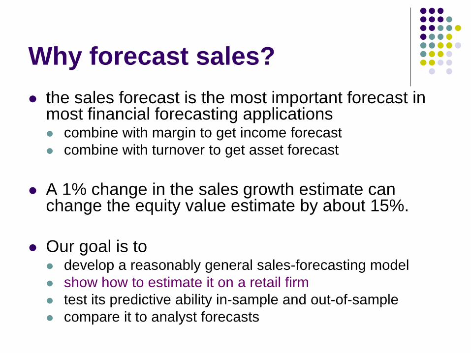
Why forecast sales? the sales forecast is the most important forecast in

most financial forecasting applications combine with margin to get income forecast combine with turnover to get asset forecast

A 1% change in the sales growth estimate can change the equity value estimate by about 15%.

Our goal is to develop a reasonably general sales-forecasting model show how to estimate it on a retail firm test its predictive ability in-sample and out-of-sample compare it to analyst forecasts

What needs to be modeled?

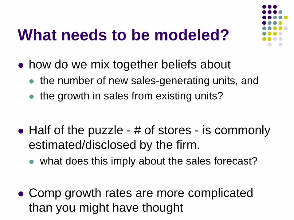
how do we mix together beliefs about the number of new sales-generating units, and the growth in sales from existing units?

Half of the puzzle - # of stores - is commonly estimated/disclosed by the firm. what does this imply about the sales forecast?

Comp growth rates are more complicated than you might have thought

The Model – sales rates / store

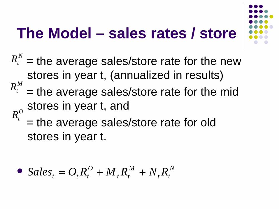
= the average sales/store rate for the new stores in year t, (annualized in results)= the average sales/store rate for the mid stores in year t, and = the average sales/store rate for old stores in year t.

NtR

MtR

OtR

Ntt

Mtt

Ottt RNRMROSales ++=

the number of stores and comps

10

15 16

10

5

4 3

10

5

4

3 2

1 2 3 4 5

close 3new

newnew

new

new

mid

midmid

mid

old

old old

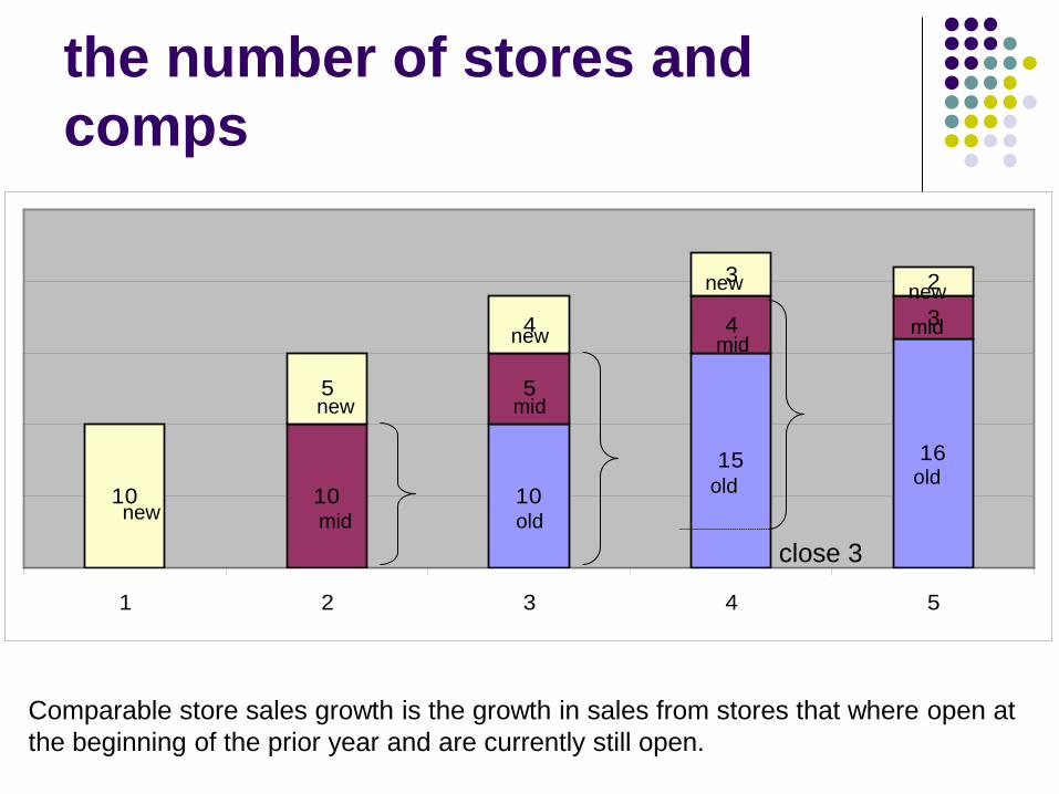
Comparable store sales growth is the growth in sales from stores that where open at the beginning of the prior year and are currently still open.

The algebra of comps

recall that Ot = Ot-1 + Mt-1 – Dt so same stores are in numerator and denominator

note that comps are sensitive to the movement of stores from mid to old (if the rates are different)

if each period then

Mtt

Ottt

Ott

t RMRDOROC

1111 )(1

−−−− +−=+

Ot

Mt RR =

Ot

Ot

t RRC

1

1−

=+

Using the comp growth to “clean up” the estimation

Ntt

Mtt

Ottt RNRMROSales ++=

but the rates are unknown. However, we know something about the evolution of the rates over time.

we know the # of stores of each type

The trick in the estimation is to account for the changes in past rates as part of the independent variable so that we can estimate the most recent rates as parameters.

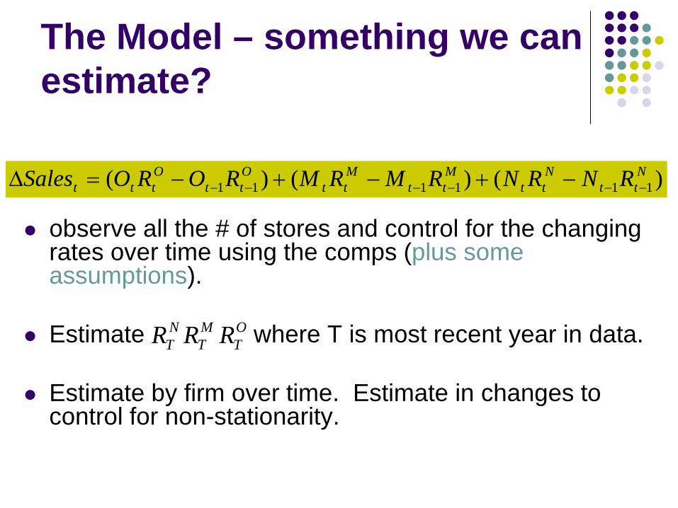
The Model – something we can estimate?

observe all the # of stores and control for the changing rates over time using the comps (plus some assumptions).

Estimate where T is most recent year in data.

Estimate by firm over time. Estimate in changes to control for non-stationarity.

)()()( 111111Ntt

Ntt

Mtt

Mtt

Ott

Ottt RNRNRMRMROROSales −−−−−− −+−+−=∆

NTR M

TR OTR

Model 1

after the end of first year, store is fully mature all rates evolve at the rate (1+Ct)

adjusting the number of beginning stores down

change in stores and rates on old+mid change in stores and rates on new

know that RtO = Rt−1

O (1+ Ct )assume that Rt

M = RtO

and RtN = Rt−1

N (1+ Ct )

NTT

NTT

OTTT

OTTTT RNRNRMORMOSales 11111 )()( −−−−− −++−+=∆

NT

T

TT

OT

T

TTTTT R

CNNR

CMOMOSales

+

−+

++

−+=∆ −−−

)1()1()()( 111

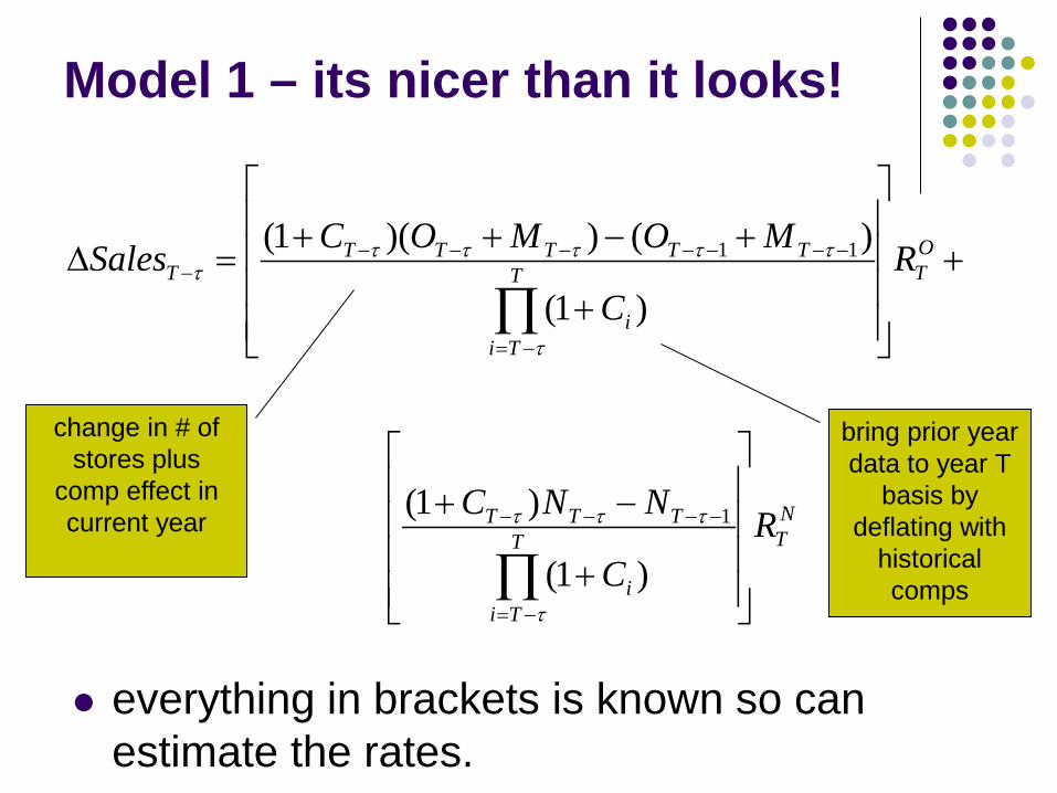
Model 1 – its nicer than it looks!

everything in brackets is known so can estimate the rates.

change in # of stores plus

comp effect in current year

bring prior year data to year T

basis by deflating with

historical comps

NTT

Tii

TTT

OTT

Tii

TTTTTT

RC

NNC

RC

MOMOCSales

+

−+

+

+

+−++=∆

∏

∏

−=

−−−−

−=

−−−−−−−−

τ

τττ

τ

ττττττ

)1(

)1(

)1(

)())(1(

1

11

RtM = kRt

O

RtN = Rt−1

N (1+ Ct )Qt , where

Qt =Ot−1 + kMt−1 − Dt

Ot

Model 2

Ot

Ot

tt RRQC

1

)1(−

=+

mid rates and new rates differ by proportion k

all rates evolve at the rate

if k > 1 (so Q>1) then prolonged new store “honeymoon period”.

if k < 1 (so Q<1) then prolonged time to maturity.

models 3-6

model 3: %∆SalesT-τ = (1+CT-τ)(1+GT-τ)-1 assumes

model 4: ∆SalesT-τ = SalesT-τ-1SGj where SGjis historical sales growth for that decile (Nissim/Penman 2001)

model 5: ∆SalesT-τ = β(∆ total # stores) + ε model 6: ∆SalesT-τ = γ1∆ existing stores +

γ2∆ new stores + ε

RtM = Rt

O = RtN

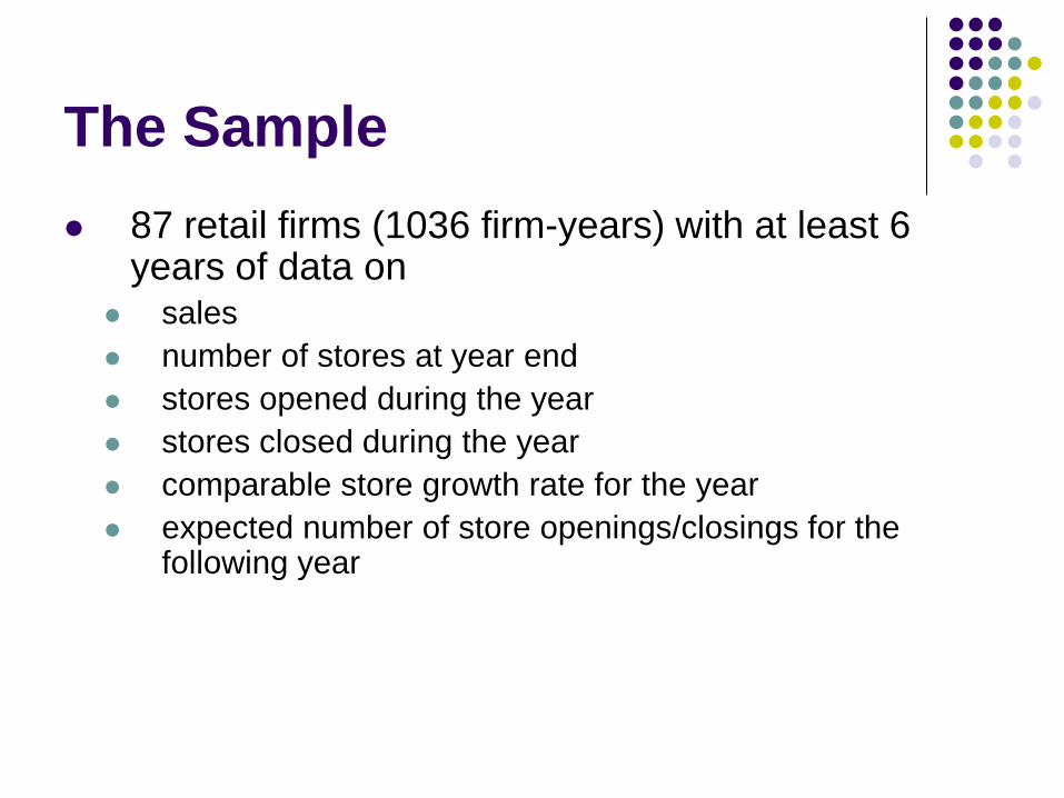
The Sample 87 retail firms (1036 firm-years) with at least 6

years of data on sales number of stores at year end stores opened during the year stores closed during the year comparable store growth rate for the year expected number of store openings/closings for the

following year

Summary Regression Results (estimated firm-by-firm)

In-Sample comparison of models

examples

old rate new rate k R2

Starbucks 1.18 0.66 k=1 98.9

Whole Foods

29.85 43.33 k=1 97.5

Walmart 111.65 322.74 k=1.2 94.0

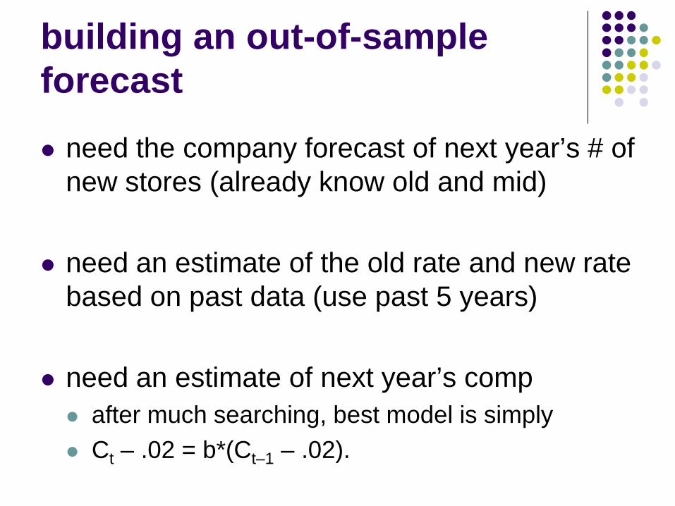
building an out-of-sample forecast

need the company forecast of next year’s # of new stores (already know old and mid)

need an estimate of the old rate and new rate based on past data (use past 5 years)

need an estimate of next year’s comp after much searching, best model is simply Ct – .02 = b*(Ct–1 – .02).

out-of-sample results

0

20

40

60

80

100

120

ibes

model1

model 1 versus analyst forecasts

median IBES analyst absolute forecast error is 3.20% of salesmedian model 1 absolute forecast error is 3.79% of sales

incremental value relative to analyst forecasts

Review of Accounting Studies

Financial Statement Analysis and Valuation: Forecasting Firm and Industry Fundamentals

October 22-23, 2010

Mendoza College of BusinessThe University of Notre Dame

Submission Deadline: May 5, 2010