Forecasting Crime: A City Level Analysis

John V. Pepper Department of Economics

University of Virginia PO Box 400184

Charlottesville, VA 22904-4182 jvp3m@virginia.edu

September 2007

Abstract: Using a common panel data set of city level crime rates from 1980-2004, I illustrate the ability of several regression models to forecast crime rates. There is considerable variability in the forecasting performance across models, cities, crimes, and forecast horizons. While there is evidence of heterogeneity across cities, heterogeneous models do not perform notably better than the homogeneous alternatives. A naïve random walk forecasting model performs relatively well for shorter run forecast horizons, but the regression models do better for longer horizons. Out of sample forecasts are sensitive to covariates, with one regression model predicting that city level crime rates will slightly increase over the remainder of the decade, and another predicting a slight drop. In the end, I find forecasting crime rates at the city level to be fragile exercise with few generalizable lessons for how best to proceed. Acknowledgements: I have benefited from the comments of Phil Cook, Jose Fernandez, Elizabeth Wittner, the University of Virginia Public Economics Lunch Group, and participants at the Committee on Law and Justice Workshop on Understanding Crime Trends. I thank Rosemary Liu for assistance in formatting and organizing the data file. The data used in this paper were assemble by Rob Fornango, and made available by the Committee on Law and Justice. The author remains solely responsible for how the data have been used and interpreted.

1

It's tough to make predictions, especially about the future.

Yogi Berra I. Introduction

For nearly three decades, criminologists have tried unsuccessfully to forecast aggregate crime

rates. Long-run forecasts have been notoriously poor. Crime rates have risen when forecasted to fall

(e.g., the mid-1980s) and have fallen when predicted to rise (e.g., the 1990s).1 Yet, despite these

difficulties, there is little relevant research to guide future forecasting efforts.

In this light, I explore some of the practical issues involved in forecasting city level crime rates

using a common panel data set. In particular, I focus on the problem of predicting future crime rates

from observed data, not the problem of predicting how different policy levers impact crime. Although

clearly important, causal questions are distinct from the forecasting question consider in this paper.

Research on cause and effect must address the fundamental identification problem that arises when

trying to predict outcomes under some hypothetical regime, say new sentencing or policing practices.

My more modest objective is to examine whether historical time-series data can be used to provide

accurate forecasts of future crime rates.

To do this, I analyze forecasts from a number of basic and parsimoniously specified mean

regression models. While the problem of effectively forecasting crime may ultimately require more

complex models, there is ample precedent for applying simple alternatives (Diebold , 1998; Baltagi,

2006).2 Thus, I focus on basic linear models that do not allow for structural breaks in the time-series

process, do not incorporate cross-state or cross crime interactions, and include only a small number of

observed covariates. Finally, I focus on point rather than interval forecasts. Sampling variability plays a

1 Land and McCall (2001) and Levitt (2004) review and critique the crime forecasting literature. 2 Diebold refers to this idea as the parsimony principle; all else equal, simple models are preferable to complex models. Certainly, imposing correct restrictions on a model should improve the forecasting performance, but even incorrect restrictions may be useful in finite samples. Simple models can be more precisely estimated, and may lessen likelihood of over-fitting the observed data at the expense of effective forecasting of unrealized outcomes. Finally, empirical evidence from other settings reveals that simpler models can do at least as well and possibly better at forecasting than more complex alternatives.

2

key role in forecasting, but a natural starting point is to examine the sensitivity of point forecasts to

different modeling assumptions. Thus, my focus is on forecasting variability across different models.

Adding confidence intervals will only increase the uncertainty associated with these forecasts.

I begin in Section 2 by considering the problem of forecasting the national homicide rate. This

homicide series lies at the center of much of the controversy surrounding the earlier forecasting

exercises that have proven so futile. Using annual data on homicide rates, I estimate a basic

autoregressive model which captures some important features of the time series variation in homicide

rates, and does reasonably well at shorter run forecasts. As for the longer run forecasts, the statistical

models clearly predict a sharp drop in crime during the 1990s, but fail to forecasts the steep rise in crime

during the late 1980s.

After illustrating the basic approach using the national homicide series, I then focus on the

problem of forecasting city level crime rates in Section 3. Using panel data on annual city level crime

rates from 1980-2000, I again estimate a series of autoregressive lag models for four different crimes --

homicide, robbery, burglary and motor vehicle theft (MVT). Data from 2001-2004 are used for out-of-

sample analyses.

The key objective is to compare the performance of various city level forecasting models. First,

I examine basic panel data models with and without covariates, and with and without autoregressive

lags. Most importantly, I contrast the homogeneous panel data model with heterogeneous models where

the process can vary arbitrarily across cities. I also consider two naïve models, one where the forecast

simply equals the city level mean or fixed effect – the best constant forecast – and the other where the

forecast equals the last observed rate – a random walk forecast. In addition to considering the basic

plausibility of the various model estimates, I examine differences in prediction accuracy and bias over

one-, two-,four-, and ten-year forecast horizons.

I find considerable variability in the parameters and forecasting performance across models,

cities, crimes, and horizons. While there is evidence of heterogeneity across cities, heterogeneous

models do not perform notably better than the homogeneous alternatives. A naïve random walk

3

forecasting model performs quite well for shorter run forecast horizons, but the regression models are

superior for longer horizon forecasts.

Finally, I use the basic homogeneous panel data models to provide point forecasts for city level

crime rates in 2005, 2006 and 2009. This out of sample forecasting exercise reveals predictions that are

sensitive to the covariate specification. All models generally indicate modest changes in city level crime

rates over the next several years. However, forecasts found using one model imply that city level crime

rates will tend to increase over the remainder of the decade, whereas forecasts from another model

imply that crime rates will fall.

In Section 4, I draw conclusions about the limitations of forecasting in general, and the specific

problems associated with forecasting crime. Forecasting city level crime rates appears to be a volatile

exercise, with few generalizable lessons for how best to proceed.

II. National Homicide Rate Trends

While my primary interest is to forecast city level crime rates, I begin by considering the national

time series in homicide rates. Some of the basic issues involved in forecasting crime can be illustrated

effectively by considering this single national time series. Attempts to forecasts this series in the 1980s

and 1990s have been notoriously inaccurate.

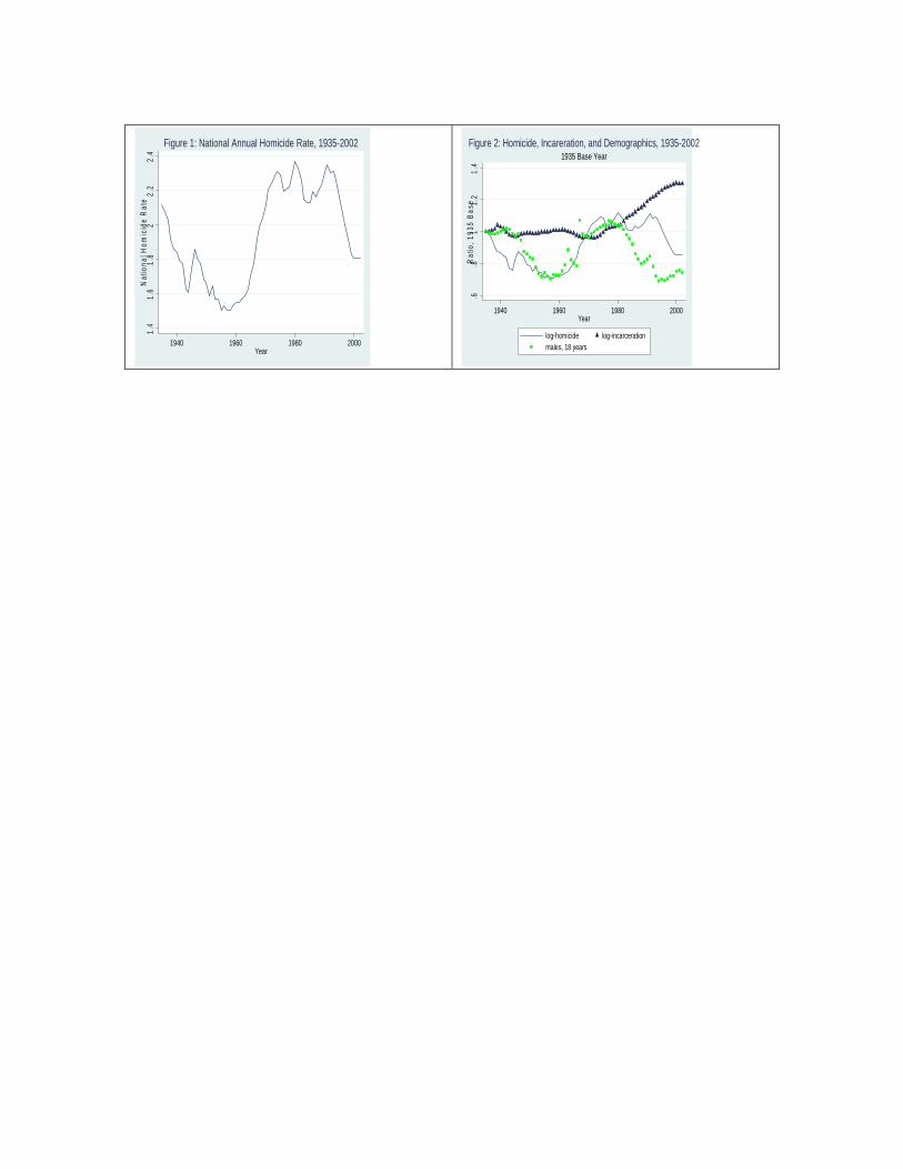
Using data on annual homicide rates per 100,000 persons from the National Center for Health

Statistics, I display the annual time series in the log rate from 1935-2002 in Figure 1. 3 The series

appears to be quite persistent over time, with some periods of fluctuation and notable turns. From 1935

until around 1960 the homicide rate tended downward, and then began sharply rising until reaching a

peak of just over 10 homicides per 100,000 (log-rate of 2.31) in 1974. Over the next 15 years, homicide

rates fluctuated between 8 and 10 per 100,000 (log rates between 2.13 and 2.33), and then unexpectedly

3 Data come from the National Center for Health Statistics, and were downloaded in January 2007 from the Bureau of Justice Statistics Historical Crime Data Series at http://www.ojp.usdoj.gov/bjs/glance/tables/hmrttab.htm. The victims of the 9/11/01 terrorist attacks are not included in this analysis.

4

began to sharply and steadily fall in the 1990s. By the end of the century, the homicide rate hit a 34 year

low of 6.1 per 100,000 (log-rate of 1.81).

A variety of demographic, economic and criminal justice factors are known to be correlated

with this series, and have been used to predict aggregate crime rates. Demographic characteristics of the

population – namely gender, age and race distributions -- have long played a primary role in crime

forecasting models (see Land and McCall, 2001). Criminal justice policies including the number of

police and the incarceration rates are also thought to be important factors in explaining aggregate crime

rates and trends. Macroeconomic variables appear to play only a modest role in explaining aggregate

crime rates, especially for violent crimes such as homicide (Levitt, 2004).

For this study, I use two primary covariates, the percent of the population that are 18 year old

males and the fraction of the population (per 100,000) that are incarcerated. Figure 2 displays the time

series for these two random variables along with the homicide rate series. All three series are

normalized to be relative to a 1935 base. This figure reveals that the fraction of young men (18 year

olds) is closely related to the homicide rate. In contrasts, the variation in incarceration rates does not

mirror the analogous variation in crime rates. Rather, incarceration rates tended to increase over the

entire century, with the sharpest increases beginning in the mid-1970s. The notable exceptions are

during peak draft years during World War II and the Vietnam War.

I follow the convention in the literature by taking the natural logarithm of the crime and

incarceration rates. I estimate the regression models using the annual data from 1935-2000, leaving out

pre-1935 data because accurate homicide rate and covariate information is not readily available, and the

post 2000 data to assess forecasting performance.

The means and standard deviations of the variables used in the analysis are displayed in Table

1. Figures for 2001-2002 are separated out, as these data are not used to estimate the model. Notice the

difference between the historical series from 1935-2000, where mean log-homicide rate equals 7.26 per

100,000 persons, and the 2001-2002 rate, which is over one point less.

5

A. The Best Linear Predictor

To forecast the homicide series in Figure 1, I fit the following autoregressive regression model:

(1.) ttttt xyyy εβγγ +++= −− 2211 ,

where yt is the log-homicide rate in year t, xt is 1xK vector of observed covariates, and εt is an iid

unobserved random variable assumed to be uncorrelated with xt.4 Finally, {γ,β} are unobserved

covariates which are consistently estimated using least-squares.

Table 2 displays estimates and standard errors from two variations on this specification: Model

A includes the AR(2) lags and Model C presents estimates from the full unrestricted specification.

Consistent with Figure 1, there is a strong autoregressive component to the series, with the period t

homicide rate being strongly associated with the lagged rates. In the unrestricted Model C, the

regression coefficients associated with the incarceration rate is positive, small and statistically

insignificant. Likewise, the coefficient on the demographic variable is statistically insignificant and

relatively small in magnitude.

B. In-Sample Forecasts

How well does this model do at forecasting crime in the 1980s and 1990s? Figure 3 presents the

predicted series under different starting dates for the forecast. In panel A, the forecasted series begins in

1981 (i.e., 1980 is assumed to be the last observed year); in Panel B the forecasts begin in 1986, in Panel

C the forecasts begin in 1991, and finally, in Panel D, the series begins in 1996. In each case, the

forecasts are dynamic in yt-1 and yt-2 ; the forecasted lagged homicide rates, not the actual rates, are

4 Several statistical tests were used to aid in the selection of the specification in Equation 1. Based on a visual inspection of the correlogram and on an augmented Dickey-Fuller test, I found no evidence of a unit root in the homicide series. Thus, there appears to be no need to difference this series. The AR(2) model was then selected using the AIC and BIC criteria, among the class of ARIMA(3,0,3) models. Finally, McDowall (2001) provides evidence favoring a linear specification over a number of nonlinear alternatives.

6

used. Importantly, these forecasts are not dynamic in the covariates; for Model C, actual covariate data

are used for all forecasts.

The forecasts beginning in 1981 (Panel A) and 1986 (Panel B) suffer the same qualitative errors

made by criminologist nearly three decades ago. In particular, the model forecasts a steady drop in

homicide rates throughout the 1980s, yet the actual rates rose in the late 1980s.

Ultimately, the ability of this model to effectively forecast crime depends on observed

relationships continuing into future periods. The model cannot effectively capture new phenomena such

as the rise or fall of new drug markets. What then should forecasters have predicted at the start of the

1990s? Are we to believe that mid-1980s was just a deviation from the norm, or that there had been a

regime shift? Normal deviations and turns in a series are notoriously difficult to predict, and the 1980s

might be nothing more. If so, then the historical time series might have been used to accurately forecast

crime in the 1990s even if it mischaracterized crime trends in the late 1980s. Instead, however, the

forecasting errors in the 1980s might have reflected a structural change in the time series process that

cannot be identified by the historical data.

With hindsight, we can see that the forecasts made for the 1990s based on the historical series

are relatively accurate. Crime is forecasted to fall (see Figure 3c), although the regression models miss

the steepness of the realized decline. Thus, the historical time series, as modeled in Equation (1), are

sufficient to predict the direction if not the full magnitude of the drop in homicide rates during the

1990s. These general patterns are consistent with the hypothesized notion of a short “bubble” in the

homicide rate that was induced by violence associated with the crack epidemic in the 1980s (Land and

McCall, 2001).

A more systematic evaluation is found by measuring the errors associated with different fixed

forecast horizons. In particular, I compute the two and five year ahead forecasts for each year from

1980-2002. Given these predictions, I then report measures of forecasts bias and accuracy. I compute

mean error (ME) as an indictor of the statistical bias of the forecasts, and the root mean squared error

(RMSE) and mean absolute error (MAE) as measures of the accuracy of the forecasts (CBO, 2005). The

7

MAE and RMSE show the size of the error without regard to sign, with RMSE giving more weight to

larger errors. If small errors are less important, the RMSE error will give the best indication of accuracy.

Also, as a different indictor of systematic one-sided error or forecasting bias, I compute the fraction of

positive errors (FPE).

Table 3 displays the realized log-homicide rates and the two- and five-year ahead forecasts for

each year from 1980 to 2002. I also include forecasts derived from a naïve random walk model that uses

the last observed rate to predict future outcomes. So, in the two-period ahead analysis, the naïve forecast

would be the rate observed two periods prior, and likewise the five-period ahead forecast is the rate in

period t-5. The bottom rows of Table 3 display the four summary measures of bias and accuracy of the

forecasts.

Several general conclusions emerge from the results displayed in this table. First, as expected,

the two period ahead forecasts are more accurate than the five-period ahead counterparts. The RMSE for

the two period ahead forecasts is about 0.10 and the MAE is around 0.09, whereas for the five period

ahead forecasts these measures are around 0.18 and 0.15 respectively. For comparison, the RMSE for

the in-sample predictions is about 0.06 (see Table 2). Second, in general, the forecasting models

outperform the naïve random walk model, and especially for the longer run forecasts. For the shorter

two period ahead forecast, the naïve model performs nearly as well as the AR(2) model in Equation (1).

For the shorter horizons, the differences in forecasting performance across these three models appear

small and, to a large degree, may reflect sampling variability. Finally, during this 23 year period, the

forecasting models consistently under predict during the period from 1989 to 1994 and over predict

homicide rates after 1995.

C. Out-of-Sample Forecasts

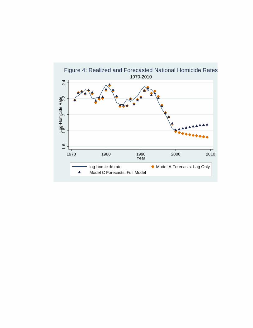
In Figure 4, I display the actual log-homicide series and the one-step- ahead predictions for each

year from 1970-2000. These in-sample predictions nearly match the realized crime rates; the regression

model closely fits the observed data.

8

I also display dynamic forecasts of the homicide rate for 2001 to 2010. For these forecasts, I assume

that last observed year is 2000.5 In this setting, forecasts of the homicide series are sensitive to

variations in the choice of explanatory variables included in the regression model. Both models predict

relatively modest changes to the homicide rate over the period, yet they have different qualitative

implications. The Model A forecasts imply that homicide rates will continue to fall during the period,

whereas the Model C forecasts suggests homicide rates will increase.

III. Forecasting City Level Crime Rates

To forecast city level crime rates, the Committee on Law and Justice (CLAJ) provided me with

a panel data set of annual crime rates in the 101 largest U. S. cities (approximately all cities with greater

than 200,000 persons) over the period 1980 to 2004.6 The data consists of rates of homicide, robbery,

burglary, and motor vehicle theft as measured by the Federal Bureau of Investigations Uniform Crime

Reports. The data also include annual measures of drug related arrest, state level incarceration rates, and

the number of police per 100,000. I supplement these data with annual county level demographic

information on the fraction of the population whom are males between 20-29 and males between 30-39,

and the natural logarithm of the total county population. As with the national series, I follow the

convention in the literature by taking the natural logarithm of the crime, incarceration and policing rates.

Using these data, I provide out-of-sample city level forecasts for 2005 and 2006. When

providing out of sample forecasts, one must either predict contemporaneous covariates or use lagged

covariates in the forecasting model. I use lagged covariates. That is, to address the practical problem

that arises when forecasting using covariates, I lag all covariates by two periods.

Given this lag structure, I estimate the models using data from 1982-2000, leaving out pre-1982

data to incorporate the lagged covariates and the post 2000 data to assess forecasting performance.

5 For the Model C forecasts, observed covariate data from 2001 and 2002 are used in the corresponding forecasts. Unobserved covariate data from 2003-2010 are assumed to be unchanged from the 2002 realizations. 6 Most of the crime data from Kansas City are missing. Thus, while there are 101 cities in this sample, Kansas City is dropped from most of the analysis.

9

Thus, for each of the 101 cities, there are 19 years of data used to estimate the parameters and four years

of data to evaluate forecasting performance. .

Summary statistics for these variables are provided in Table 4. As in the national homicide

series, the pre-2000 average crime rates are notably different than the analogous rates from 2001-2004.

The average log-homicide rate, for example, is 2.55 in the 1982-2000 period, and 2.31 from 2001-2004.

Likewise, the mean log-incarceration rates from 1982-2000 is 5.50, much less than the average rate of

6.04 from 2001-2004.

By using a common data set and specification, I provide insights into how different regression

models perform in forecasting city level crime rates. I examine the suitability of these models in several

ways. First, in Section A, I describe the basic model, and examine the estimated parameters. I find

considerable variability in the parameter estimates even amongst the models that are restricted to be the

same across all cities. In Section B, I assess forecast performance of these models to one-, two-, four-

and ten-year ahead forecasts of city level crime rates. I compare the performance of a basic

homogeneous panel data regression model with a flexible heterogeneous alternative. These results show

much variability in the forecast performance of various models across cities, crimes and forecasts

horizons. The heterogeneous models are not always superior. For short run forecasts, a naïve random

walk forecasting model appears to perform well, whereas the homogeneous models seems to perform

relatively well for longer run forecasts.

In Section C, I provide out-of-sample forecast of the city level crime rates using the

homogeneous dynamic panel data model. As with the forecasted national homicide rate series, I find the

qualitative predictions are sensitive to the underlying model.

A. Best Linear Predictor

To forecast city level crime rates, I begin by considering the following dynamic panel data

model:

10

(2.) itititiit xyy ενβγ +++= −− 2,1,1

where yit is the log-crime rate in state i for year t, xit is the set of observed covariates, ν i reflects

unobserved city level fixed effects, and εit is an iid unobserved random variable, independent of x and ν.

The unknown parameters, {γ, β} are estimated by ordinary least-squares.7

Table 5 displays estimates and standard errors from three variations on the specification in

Equation (2.): Model A includes the autoregressive lag, β=0; Model B includes the covariates, γ = 0;

and Model C is the full unrestricted specification. All three specifications include the city level fixed

effects, νi.

The estimates from Model A reveal a notable autoregressive component in the four crime rate

series, such that the period t crime rate is strongly associated with the lagged rate. There is, however,

much variation in this autoregressive coefficient across the four crimes, varying from 0.452 for

homicide to 0.923 for burglary. The autoregressive coefficient estimate uniformly falls but still remains

substantial and statistically significant when covariates are added to the model.

The association between crime and covariates seems to generally conform to expectations. Log-

crime rates increase with the natural logarithm of drug arrests and the fraction of young men, and

decrease with the log-incarceration rates and the log-number of police. Again, there is much variability

across crimes and specifications. For example, in Model B, the absolute elasticity of the crime rate with

respect to the per-capita number of police ranges from a high of 0.362 for homicide to a low of 0.174 for

burglary.

In panel data, the forecast precision depends both on the stability of the process over time, and

across cross-sectional units. Variation in the slope parameters across the cross-sectional units may

compromise the ability of the homogeneous dynamic panel data model in Equation (2) to accurately

7 The OLS estimator will generally be inconsistent for fixed-T. Alternative instrumental variable estimators are, under certain assumptions, consistent in this situation. I did not evaluate the forecasts found under alternative estimators.

11

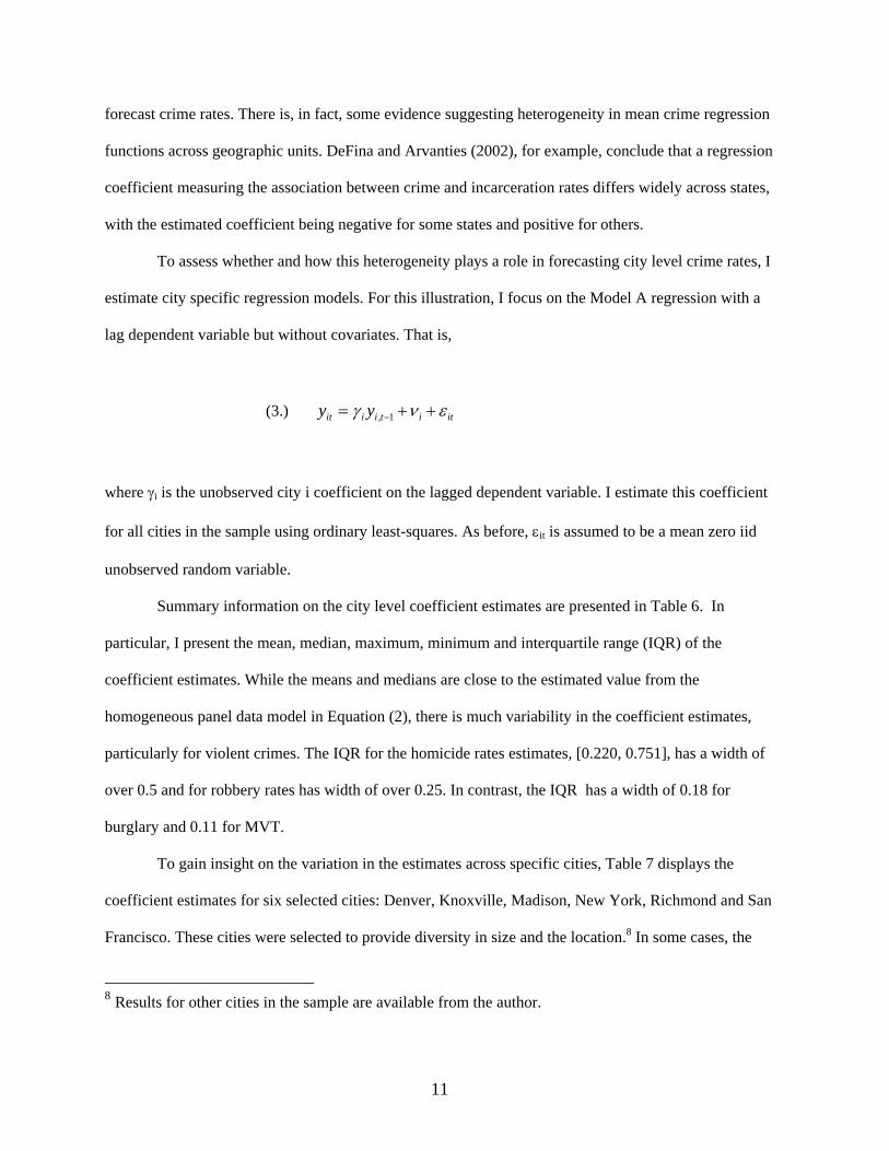
forecast crime rates. There is, in fact, some evidence suggesting heterogeneity in mean crime regression

functions across geographic units. DeFina and Arvanties (2002), for example, conclude that a regression

coefficient measuring the association between crime and incarceration rates differs widely across states,

with the estimated coefficient being negative for some states and positive for others.

To assess whether and how this heterogeneity plays a role in forecasting city level crime rates, I

estimate city specific regression models. For this illustration, I focus on the Model A regression with a

lag dependent variable but without covariates. That is,

(3.) ititiiit yy ενγ ++= −1,

where γi is the unobserved city i coefficient on the lagged dependent variable. I estimate this coefficient

for all cities in the sample using ordinary least-squares. As before, εit is assumed to be a mean zero iid

unobserved random variable.

Summary information on the city level coefficient estimates are presented in Table 6. In

particular, I present the mean, median, maximum, minimum and interquartile range (IQR) of the

coefficient estimates. While the means and medians are close to the estimated value from the

homogeneous panel data model in Equation (2), there is much variability in the coefficient estimates,

particularly for violent crimes. The IQR for the homicide rates estimates, [0.220, 0.751], has a width of

over 0.5 and for robbery rates has width of over 0.25. In contrast, the IQR has a width of 0.18 for

burglary and 0.11 for MVT.

To gain insight on the variation in the estimates across specific cities, Table 7 displays the

coefficient estimates for six selected cities: Denver, Knoxville, Madison, New York, Richmond and San

Francisco. These cities were selected to provide diversity in size and the location.8 In some cases, the

8 Results for other cities in the sample are available from the author.

12

city specific coefficients estimates are similar to those found from the homogeneous panel data model in

Equation (2), but in others the estimates are notably different. Consider, for example, the coefficient

estimates found using the robbery rate series. The autoregressive coefficient estimates found using the

homogeneous model is 0.759, similar to the city specific estimates found for Knoxville (0.76),

Richmond (0.73) and Madison (0. 65). In contrast, the two sets of estimates are notably different for

Denver (0.94), New York (1.13) and San Francisco (0.94).

This heterogeneity in the lagged coefficient would seem to have important implications for our

ability to accurately forecast city level crime rates. The heterogeneous estimators have the desirable

property of allowing for differences across cities. Yet, one might fit the observed the data quite well at

the expense of forecasting the future very poorly. In particular, estimates from the city specific models

will be less precise, and may be highly influenced by short run bubbles and other departures from a

“stationary” trend. In this application, where the time series includes 19 observations per city, this

tradeoff seems especially important. Ultimately, whether and how the heterogeneity in crime rate

regression models impacts the forecasting performance of these models is unknown. I take up that issue

in the next section.

B. In-Sample Forecasts

How well does the homogeneous panel data model do at forecasting crime rates? Given my

focus on two period ahead forecasts, I begin by using this model to predict the 2003 and 2004 crimes

rates for each city. Recall, that the models are estimated using data through 2000, so forecasts of the

2003 and 2004 rates constitute an “out of sample” forecasts for which we observe the realized crime

rate. For this exercise, I treat 2002 as the last observed year, so that predictions for 2003 are one-period

ahead forecasts and predictions for 2004 are two-steps ahead. For each city crime pair, I compute

forecasts using the restricted Model A and the unrestricted Model C.

Forecasts for the six selected cities, Denver Knoxville, Madison, New York, Richmond and San

Francisco, are presented in Table 8. The results vary across crimes, cities, time and model. The forecast

13

errors are generally smaller in 2003 than 2004, and generally larger for homicide than other crimes.

However, models that do relatively well at predicting a particular crime in a particular city need not

provide accurate predictions about other crimes, in other time periods or cities. For example, both

models do poorly at forecasting the 2003 homicide rate in Madison, yet are relatively accurate at

forecasting the 2004 homicide rate, as well as the robbery rate in 2003 and 2004. Likewise, the models

do well at predicting the 2003 homicide and MVT rates in Denver, but do poorly at predicting robbery

and burglary. There is also variation across forecasting models. In general, Model A appears to provide

more accurate forecasts, but there are many notable exceptions (e.g., the 2003 homicide rate in

Knoxville).

To provide a more systematic assessment of the capabilities of these models, I compute basic

summary measures of the errors in forecasting crime in every city in the sample. Table 9 displays the

mean error, the fraction of positive errors, the RMSE and MAE for forecasts from Model A, Model C,

and a naïve random walk forecasting model where the 2002 rate is used as the prediction for 2003 and

2004.

In examining these results, it is useful to first compare the summary measures across different

crimes. The models do relatively poorly at forecasting homicide. The RMSE and MAE for the 2003

homicide forecasts are around 0.40 and 0.25, substantially larger than analogous measures found for the

other three crime rates. These relatively large errors would seem to reflect the wide variation in the city

specific coefficient estimates found in Section A above (see Table 6 and 7).

Comparing the results across the different models is also instructive. For these one- and two-

year ahead predictions, the naïve random walk forecasts seem to be at least as accurate as the regression

model forecasts. In other words, for shorter run forecasts, the basic panel data models do no better, on

average, than simply guessing that next year's crime rate will be the same as this year's. In terms of the

two regression models, Model A does at least as well if not better than the unconstrained Model C.

Moreover, these models seem to lead to qualitatively different prediction errors. The fraction of positive

errors for Model A is greater than one-half, implying that the model tends to predict crime rates in

14

excess of the realized outcomes, For Model C, the fraction positive is always less than 0.50, suggesting

predictions tend to fall short of the realized crimes rates.

Finally, notice that errors are slightly larger for the one-step ahead 2003 prediction than the

2004 two-step ahead predictions. This paradoxical result can be explained by the forecasting error from

a single city, Louisville. The 2003 realizations for Louisville were outliers that were not repeated again

in 2004. As a result, 2003 forecast errors were substantially inflated. For example, the log-MVT forecast

is 6.70 whereas the realized rate is 4.76, for a forecast error of nearly 2.0. No other absolute forecast

error for log-MVT in 2003 exceeded 0.36. If we remove Louisville, the RMSE for the 2003 forecasts

made from Model A falls to 0.31 for log-homicide, to 0.15 for log-robbery, to 0.09 log-burglary, and to

0.14 for log-MVT. The analogous figures for the 2004 forecasts errors barely change. Thus, except for

Louisville, these summary measures imply that the forecast errors are smaller in 2003 than 2004.

An important objective of this paper is to assess how the dynamic panel data model in Equation

(2) performs relative to alternative models, and most notably the heterogeneous model in Equation (3).9

The two models can produce very different predictions.

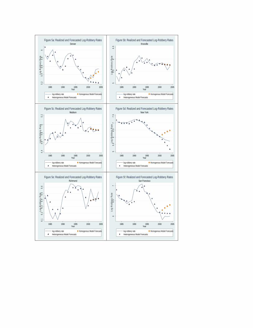
Insights into the primary issues are found by comparing forecasts for a particular crime across

different cities. Figure 5 displays the log-robbery time series and forecasts for the six cities analyzed

above (see Tables 7 and 8). For each city, I display dynamic forecasts that start in 2001 and end in 2004

using both the homogeneous and the heterogeneous models. The one-step- ahead predictions from the

heterogeneous model for each year from 1982-2000 are also displayed. These in-sample predictions

nearly match the realized crime rates; the heterogeneous model closely fits the observed data.

For the three cities where the coefficient estimates from the two models are similar, namely

Knoxville, Madison and Richmond, the two forecasts are nearly identical and seem to provide accurate

9 There are many other related models, estimators and approaches one might consider. See Baltagi (2006) for examples of forecasting models and estimators within the same structure. Model averaging techniques similar to those described in this volume by Durlauf, Navarro and Rivers (2006) have also been shown to be effective at reducing forecasting errors. Finally, one might consider using entirely different approaches, such as the prediction market forecasting techniques described by Gürkaynak and Wolfers (2006).

15

four period ahead predictions of general trends and, to some extent, the levels in log-robbery rates. The

most striking results are found in the three cities where the autoregressive coefficient estimates are

notably different across the two models, Denver (0.94), New York (1.13) and San Francisco (0.94).

Forecasts of robbery rates for these cities are sensitive to the underlying model. In particular, for these

three cities the homogeneous model suggests an increase in robbery rates over the four-year period,

whereas the heterogeneous model leads to the opposite conclusion. Realized robbery rates over this four

year period closely track the forecasts from the homogeneous model in Denver, from the heterogeneous

model in San Francisco, and lie between the two forecasts for New York.

Clearly, the heterogeneous model does not provide uniformly superior out-of-sample forecasts.

Table 10 displays summary measures of how these different models perform on average across all cities

and for different forecasts horizons. In addition to analyzing the forecasting performance of the models

in Equations (2) and (3), I also consider two naïve models, one where the forecast equals the city level

mean or fixed effect – the best constant forecast – and the other where the forecast equals the last

observed rate – the random walk forecast. Finally, I display the RMSE from the one-step ahead

forecasts that, in practice, is only feasible if the period t-1 realization is known (or perfectly forecasted).

Each model is used to provide forecasts of annual crime rates for three different overlapping

horizons, 2003-04, 2001-04, and 1995-04, and three different starting points, 2002, 2000 and 1994.

Thus, dynamic forecasts starting in 1994 are used to make 10 year-ahead predictions for the 2004 crime

rate. Importantly, these forecasts are not dynamic in the covariates; for Model C, actual covariate data

are used for all forecasts, even those that go beyond two year ahead predictions.

Many of the findings reported in this table confirm the earlier results. In particular, for shorter

run forecasts, the restricted Model A seems to do at least as well as the unrestricted Model C, and both

of these homogeneous models provide slightly less accurate forecasts than the naïve random walk

model. As before, these differences are modest and may simply reflect sampling variability rather than

true differences in forecasting performance.

16

In both cases, however, these patterns are not consistent across forecast horizons; models that

work relatively well for the shorter run do not necessarily provide accurate forecasts for longer horizons.

Long-horizon random walk forecasts, for example, perform poorly. The RMSE for the random walk

forecasts of homicide rates in 1995-2004, for instance, is 0.52, much greater than the RMSE of 0.41

found using the sample average (i.e., the best constant predictor), and Model A, where the RMSE is

0.39.

Likewise, for longer run forecasting problems, the unrestricted Model C provides more accurate

forecasts than the restricted alternative. For example, the RMSE for the 1995-2004 forecasts of the

homicide rate using the unrestricted Model C is 0.33, 0.06 less than the analogous RMSE of the

forecasts made from the restricted Model A. This finding, however, may reflect the fact that the long-

run (over two year forward) Model C forecasts utilize realized covariate data. In practice, the necessary

covariate data will not be observed.

Finally, the added flexibility of the heterogeneous forecasting model in Equation (3.) leads to

some improvements in forecasting accuracy. As might be expected, the results are especially striking

for homicide, where there is evidence of much heterogeneity in the parameter estimates. Assuming the

2002 log-homicide rate is the last observed data point, the RMSE for the 2003-04 forecasts is 0.37 using

the homogeneous Model A and 0.19 using the heterogeneous alternative.

For the other crimes, however, the forecasting gains from the heterogeneous model are less

pronounced. For example, the RMSE for forecast of burglary rates in 2003-04 is 0. 16 for both models,

and the analogous RMSE for MVT is 023 for the homogeneous model and 0.19 for the heterogeneous

alternative. Except for the homicide series, the efficiency gains from the homogeneous model appear to

nearly offset any biases due to heterogeneities.

C. Out-of-Sample Forecasts

As noted above, I forecasts city level crime rates using the observations through 2004. For this

illustration, I use the panel data models from Equation (2.) to provide forecasts of city level crime rates

17

for 2005 and 2006. I also use Model A to forecasts crime rates in 2009. Without covariate data over this

period, long-run Model C forecasts are not feasible.

In Table 11, I present these out of sample forecasts for the six selected cities analyzed

throughout this paper. Except for New York City, the forecasted changes across these six cities are

generally modest. For example, the log-robbery rates in Denver, Knoxville, and Madison are all

predicted to change by less than 0.03 points over the 5-year period from 2004 to 2009. During the

preceding five years, from 1999-2004, log-robbery rates increased by 0.23 in Denver and 0.04 in

Madison, and decreased by 0.14 in Knoxville.

The specific changes vary by city and by crime. To see this, notice the five year ahead forecasts.

In San Francisco, log-robbery rates are forecasted to increase by 0.38 points, whereas forecasts for the

other three crime rates are slightly less than the 2004 levels. In Madison, log-homicide rates are

forecasted to increase by 0.31 and log-MVT rates by 0.15, whereas the log-crime rates for both robbery

and burglary are forecasted to drop over the same period.

Finally, there are notable differences in the predictions made from the two models. In several

cases, Model A implies an increase in crime whereas Model C predicts a slight drop, and in nearly every

case the Model A forecasts exceed the Model C counterparts.

Overall patterns regarding these forecasts can be found by examining Table 12, which displays

summary measures for the forecasts in every city. In particular, for each crime and each forecast period,

I report the mean forecast, the mean predicted change, the fraction of positive predicted changes, the

IQR of the predicted change, and the mean absolute predicted change.

The results in this table confirm that Models A and C provide different pictures about what to

expected for crime in large cities over this period. Forecasts made using Model A generally imply

modest increases (e.g., homicide) or little overall change (e.g., burglary) in city level crime rates

throughout the reminder of this decade. Forecasts made using Model C paint a different picture, with

crime rates continuing to fall, in general, over the period. For example, the IQR in the forecasted

change in log-robbery rates from 2004 to 2006 is [0.02, 0.21] when using model A but is [-0.20, 0.02]

18

when using Model C. Likewise, the fraction of cities forecasted to see increases in the robbery rate is

82% under Model A, but only 36% in Model C. Finally, Model C generally predicts slightly larger

absolute changes in the crime rates, and both predict much larger absolute changes in the homicide rates

than the other three crimes.

Forecasts of the log-crime rate series are sensitive to variation in the choice of explanatory

variables in the regression model. That is, whether one concludes that city level crime rates will increase

or decrease based on models of this type depends on which control variables are included.

This variability in the forecasts is difficult to reconcile given the current state of the literature.

As far as I can tell, there is almost no research on how best to forecast crime, and there is much

disagreement about the proper set of covariates to include. The limited results presented in Section B

suggest that Model A provides somewhat more accurate forecasts for one and two year horizons. If true,

this would imply that city level crime rates will tend to increase over the period. Yet, these results also

reveal that for short run forecasts the naïve random walk model provides slightly more accurate

forecasts than either panel data model. That is, for these short run forecasts, we might not be able to do

better than the predicting that tomorrow will look like today.

IV. Conclusions

In this paper, I compare the forecasting performance of a basic homogeneous model to the

heterogeneous counterpart using the city level panel data provided by CLAJ. The results reveal the

fragility of the forecasting exercise. Seemingly minor changes to a model can produce qualitatively

different forecasts and models that appear to provide sound forecasts in some scenarios do poorly in

others. In the end, the naïve random walk forecasts that tomorrow will be like today does quite well

relative to the linear time-series models, especially for shorter run forecast horizons.

Two factors contribute to the variability and uncertainty illustrated in this paper. First,

forecasting is an inherently difficult undertaking. Social phenomena such as crime can sometimes

evolve in subtle but substantial ways that are very difficult to identify using historical data and can take

19

a long time to understand. Forecasts are invariably error ridden around turning points, especially when

these movements are largely the result of external events that are themselves unpredictable.

Second, there lacks a well-developed research program on the problem of forecasting crime.

For further headway to be made there needs to be a focused and sustained research effort. Periodic

efforts to forecast crime or analyze forecasting models cannot hope to provide meaningful guidance.

Effective forecasts of social processes that evolve over time would seem to require a scientific process

that evolves as well.

20

References:

Baltagi, Badi H. (2006). “Forecasting with Panel Data,” Syracuse University, Center for Policy Research Working Paper, No. 91.

Congressional Budget Office, (2005). CBO’s Economic Forecasting Record: An evaluation of the economic forecasts CBO made from January 1976 through January 2003. http://www.cbo.gov/ftpdocs/68xx/doc6812/10-25-EconomicForecastingRecord.pdf

DeFina, Robert H. and Thomas M.Arvanites, (2002). “The Weak Effect of Imprisonment

on Crime: 1971-1998,” Social Science Quarterly Vol. 83, Issue 3, pp. 635- Diebold, Francis X. (1998). Elements of Forecasting. South-Western College Publishing,

Cincinnati, OH. Durlauf, Steven, Salvardor Navarro and David A. Rivers, (2006). “Notes on the

Econometric Analysis of Crime,” working paper. Gürkaynak,Refet and Justin Wolfers, (2006). “Macroeconomic Derivatives: An Initial

Analysis of Market-Based Macro Forecasts, Uncertainty, and Risks,” NBER working Paper, No. 11929.

Land, Kenneth C. and Patricia L. McCall, (2001). “The Indeterminacy of Forecasts of

Crime Rates and Juvenile Offenses,” in Juvenile Crime, Juvenile Justice. National Research Council and Institute of Medicine, Panel on Juvenile Crime: Prevention, Treatment, and Control. Joan McCord, Cathy Spatz Widom, and Nancy A. Crowell, eds. Committee on Law and Justice and Board on Children, Youth, and Families. Washington, DC: National Academy Press.

Levitt, Steven D. (2004). “Understanding Why Crime Fell in the 1990s: Four Factors that

Explain the Decline and Six that Do Not,” Journal of Economic Perspective, 18(1), Winter 2004, pp. 163–190

McDowall, D. (2002). “Tests of nonlinear Dynamics in the U.S. Homicide Time Series, and Their

Implications,” Criminology, 40(3), 722-736.

1.4

1.6

1.8

22.

22.

4N

atio

nal H

omic

ide

Rat

e

1940 1960 1980 2000Year

Figure 1: National Annual Homicide Rate, 1935-2002

.6.8

11.

21.

4R

atio

, 193

5 Ba

se

1940 1960 1980 2000Year

log-homicide log-incarceration males, 18 years

1935 Base YearFigure 2: Homicide, Incareration, and Demographics, 1935-2002

1.8

22.

22.

4Lo

g-H

omic

ide

Rat

e

1970 1980 1990 2000Year

log-homicide rate Model A Forecasts: Lag OnlyModel B Forecasts: Full Model

Dynamic Forecasts: 1981-2002Figure 3a: Realized and Forecasted Homicide Rates

1.8

22.

22.

4Lo

g-H

omic

ide

Rat

e

1970 1980 1990 2000Year

log-homicide rate Model A Forecasts: Lag OnlyModel B Forecasts: Full Model

Dynamic Forecasts: 1986-2002Figure 3b: Realized and Forecasted Homicide Rates

1.8

22.

22.

4Lo

g-H

omic

ide

Rat

e

1970 1980 1990 2000Year

log-homicide rate Model A Forecasts: Lag OnlyModel B Forecasts: Full Model

Dynamic Forecasts: 1991-2002Figure 3c: Realized and Forecasted Homicide Rates

1.8

22.

22.

4Lo

g-H

omic

ide

Rat

e

1970 1980 1990 2000Year

log-homicide rate Model A Forecasts: Lag OnlyModel B Forecasts: Full Model

Dynamic Forecasts: 1996-2002Figure 3d: Realized and Forecasted Homicide Rates

1.

61.

82

2.2

2.4

Log-

Hom

icid

e R

ate

1970 1980 1990 2000 2010Year

log-homicide rate Model A Forecasts: Lag OnlyModel C Forecasts: Full Model

1970-2010Figure 4: Realized and Forecasted National Homicide Rates

5.2

5.4

5.6

5.8

6Lo

g-R

obbe

ry R

ate

1985 1990 1995 2000 2005Year

log-robbery rate Homogenous Model ForecastsHeterogeneous Model Forecasts

DenverFigure 5a: Realized and Forecasted Log-Robbery Rates

55.

56

6.5

Log-

Rob

bery

Rat

e

1985 1990 1995 2000 2005Year

log-robbery rate Homogenous Model ForecastsHeterogeneous Model Forecasts

KnoxvilleFigure 5b: Realized and Forecasted Log-Robbery Rates

4.4

4.6

4.8

55.

2Lo

g-R

obbe

ry R

ate

1985 1990 1995 2000 2005Year

log-robbery rate Homogenous Model ForecastsHeterogeneous Model Forecasts

MadisonFigure 5c: Realized and Forecasted Log-Robbery Rates

55.

56

6.5

77.

5Lo

g-R

obbe

ry R

ate

1985 1990 1995 2000 2005Year

log-robbery rate Homogenous Model ForecastsHeterogeneous Model Forecasts

New YorkFigure 5d: Realized and Forecasted Log-Robbery Rates

6.1

6.2

6.3

6.4

6.5

6.6

Log-

Rob

bery

Rat

e

1985 1990 1995 2000 2005Year

log-robbery rate Homogenous Model ForecastsHeterogeneous Model Forecasts

RichmondFigure 5e: Realized and Forecasted Log-Robbery Rates

66.

57

Log-

Rob

bery

Rat

e

1985 1990 1995 2000 2005Year

log-robbery rate Homogenous Model ForecastsHeterogeneous Model Forecasts

San FranciscoFigure 5f: Realized and Forecasted Log-Robbery Rates

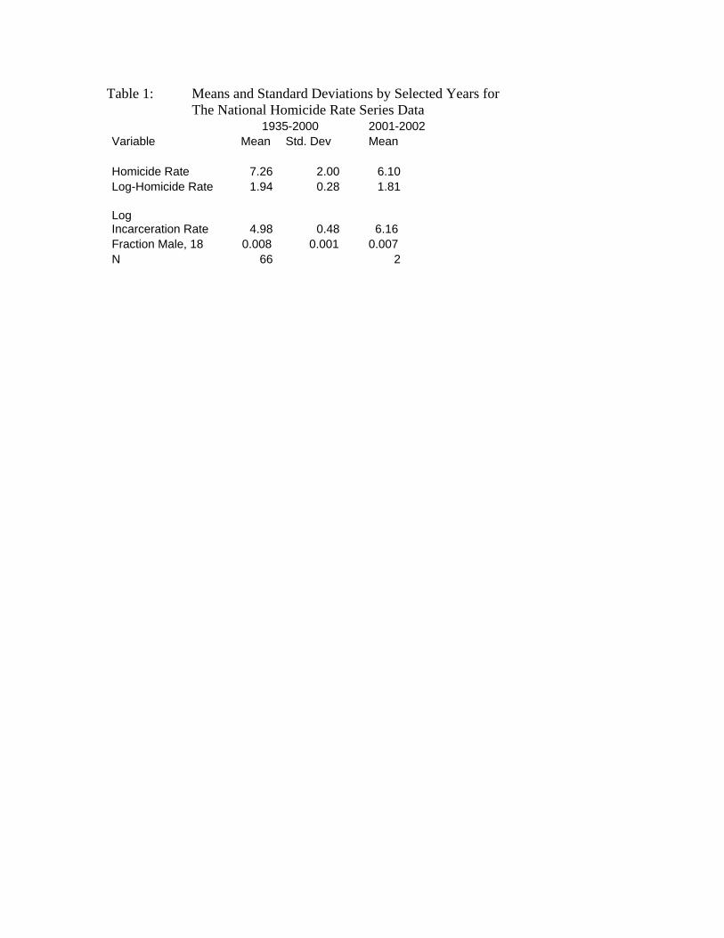
Table 1: Means and Standard Deviations by Selected Years for The National Homicide Rate Series Data

1935-2000 2001-2002 Variable Mean Std. Dev Mean Homicide Rate 7.26 2.00 6.10Log-Homicide Rate 1.94 0.28 1.81 Log Incarceration Rate 4.98 0.48 6.16 Fraction Male, 18 0.008 0.001 0.007 N 66 2

Table 2: National Homicide Rate Regression Model Estimates and Standard Errors, A C yt-1 1.46

(0.12) 1.42 (0.12)

y t-2 -0.50 (0.12)

-0.48 (0.13)

Ln(inc) 0.01 (0.03)

Fraction Male, 18

11.38 (11.25)

RMSE 0.06 0.06 R2 0.96 0.96 N 64 64 Notes: Ln(inc) ª log-incarceration rate; yt ª log-homicide rate in year t.

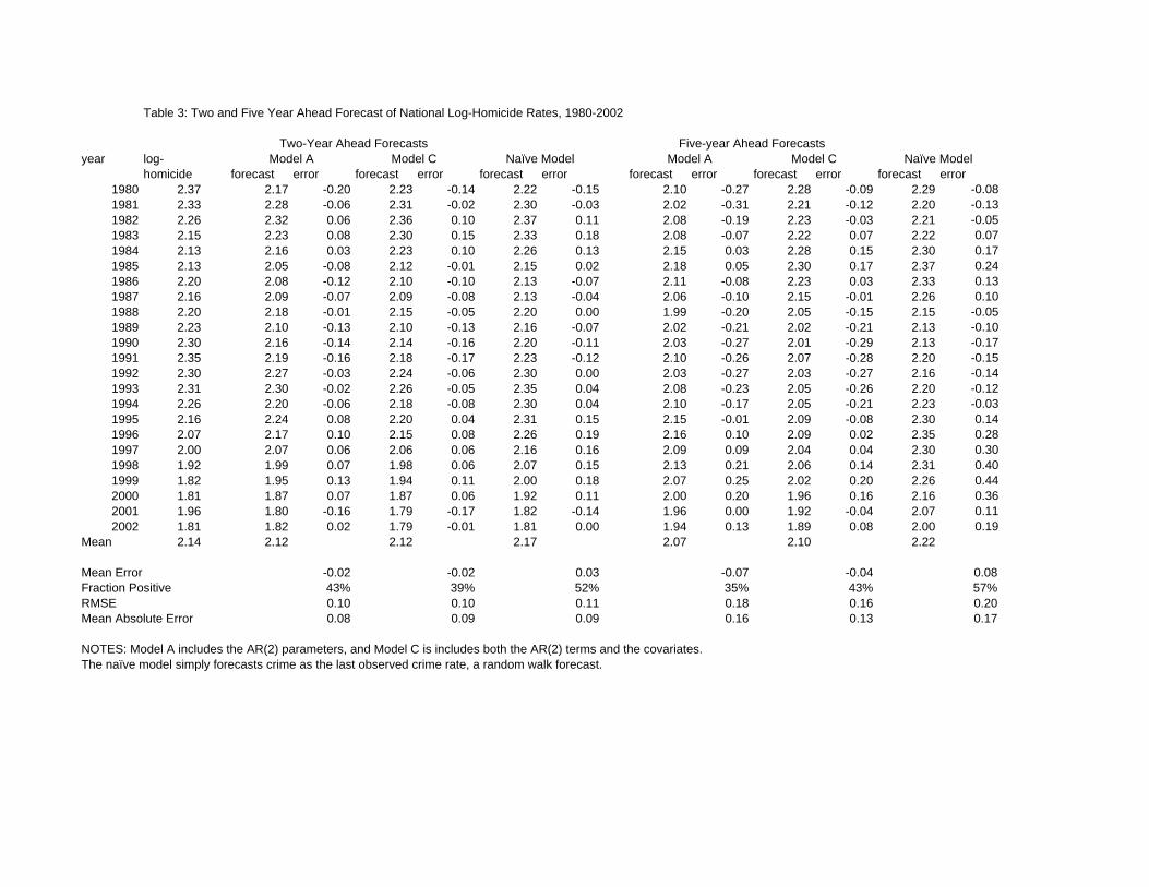
Table 3: Two and Five Year Ahead Forecast of National Log-Homicide Rates, 1980-2002

year log-homicide forecast error forecast error forecast error forecast error forecast error forecast error

1980 2.37 2.17 -0.20 2.23 -0.14 2.22 -0.15 2.10 -0.27 2.28 -0.09 2.29 -0.081981 2.33 2.28 -0.06 2.31 -0.02 2.30 -0.03 2.02 -0.31 2.21 -0.12 2.20 -0.131982 2.26 2.32 0.06 2.36 0.10 2.37 0.11 2.08 -0.19 2.23 -0.03 2.21 -0.051983 2.15 2.23 0.08 2.30 0.15 2.33 0.18 2.08 -0.07 2.22 0.07 2.22 0.071984 2.13 2.16 0.03 2.23 0.10 2.26 0.13 2.15 0.03 2.28 0.15 2.30 0.171985 2.13 2.05 -0.08 2.12 -0.01 2.15 0.02 2.18 0.05 2.30 0.17 2.37 0.241986 2.20 2.08 -0.12 2.10 -0.10 2.13 -0.07 2.11 -0.08 2.23 0.03 2.33 0.131987 2.16 2.09 -0.07 2.09 -0.08 2.13 -0.04 2.06 -0.10 2.15 -0.01 2.26 0.101988 2.20 2.18 -0.01 2.15 -0.05 2.20 0.00 1.99 -0.20 2.05 -0.15 2.15 -0.051989 2.23 2.10 -0.13 2.10 -0.13 2.16 -0.07 2.02 -0.21 2.02 -0.21 2.13 -0.101990 2.30 2.16 -0.14 2.14 -0.16 2.20 -0.11 2.03 -0.27 2.01 -0.29 2.13 -0.171991 2.35 2.19 -0.16 2.18 -0.17 2.23 -0.12 2.10 -0.26 2.07 -0.28 2.20 -0.151992 2.30 2.27 -0.03 2.24 -0.06 2.30 0.00 2.03 -0.27 2.03 -0.27 2.16 -0.141993 2.31 2.30 -0.02 2.26 -0.05 2.35 0.04 2.08 -0.23 2.05 -0.26 2.20 -0.121994 2.26 2.20 -0.06 2.18 -0.08 2.30 0.04 2.10 -0.17 2.05 -0.21 2.23 -0.031995 2.16 2.24 0.08 2.20 0.04 2.31 0.15 2.15 -0.01 2.09 -0.08 2.30 0.141996 2.07 2.17 0.10 2.15 0.08 2.26 0.19 2.16 0.10 2.09 0.02 2.35 0.281997 2.00 2.07 0.06 2.06 0.06 2.16 0.16 2.09 0.09 2.04 0.04 2.30 0.301998 1.92 1.99 0.07 1.98 0.06 2.07 0.15 2.13 0.21 2.06 0.14 2.31 0.401999 1.82 1.95 0.13 1.94 0.11 2.00 0.18 2.07 0.25 2.02 0.20 2.26 0.442000 1.81 1.87 0.07 1.87 0.06 1.92 0.11 2.00 0.20 1.96 0.16 2.16 0.362001 1.96 1.80 -0.16 1.79 -0.17 1.82 -0.14 1.96 0.00 1.92 -0.04 2.07 0.112002 1.81 1.82 0.02 1.79 -0.01 1.81 0.00 1.94 0.13 1.89 0.08 2.00 0.19

Mean 2.14 2.12 2.12 2.17 2.07 2.10 2.22

Mean Error -0.02 -0.02 0.03 -0.07 -0.04 0.08Fraction Positive 43% 39% 52% 35% 43% 57%RMSE 0.10 0.10 0.11 0.18 0.16 0.20Mean Absolute Error 0.08 0.09 0.09 0.16 0.13 0.17

NOTES: Model A includes the AR(2) parameters, and Model C is includes both the AR(2) terms and the covariates.The naïve model simply forecasts crime as the last observed crime rate, a random walk forecast.

Naïve ModelTwo-Year Ahead Forecasts

Model A Model C Five-year Ahead Forecasts

Model A Model CNaïve Model

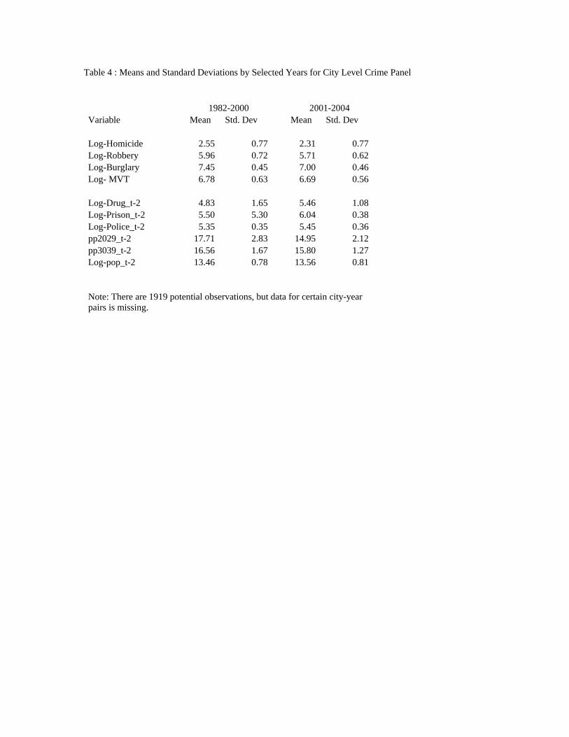
Table 4 : Means and Standard Deviations by Selected Years for City Level Crime Panel 1982-2000 2001-2004 Variable Mean Std. Dev Mean Std. Dev Log-Homicide 2.55 0.77 2.31 0.77 Log-Robbery 5.96 0.72 5.71 0.62 Log-Burglary 7.45 0.45 7.00 0.46 Log- MVT 6.78 0.63 6.69 0.56 Log-Drug_t-2 4.83 1.65 5.46 1.08 Log-Prison_t-2 5.50 5.30 6.04 0.38 Log-Police_t-2 5.35 0.35 5.45 0.36 pp2029_t-2 17.71 2.83 14.95 2.12 pp3039_t-2 16.56 1.67 15.80 1.27 Log-pop_t-2 13.46 0.78 13.56 0.81 Note: There are 1919 potential observations, but data for certain city-year pairs is missing.

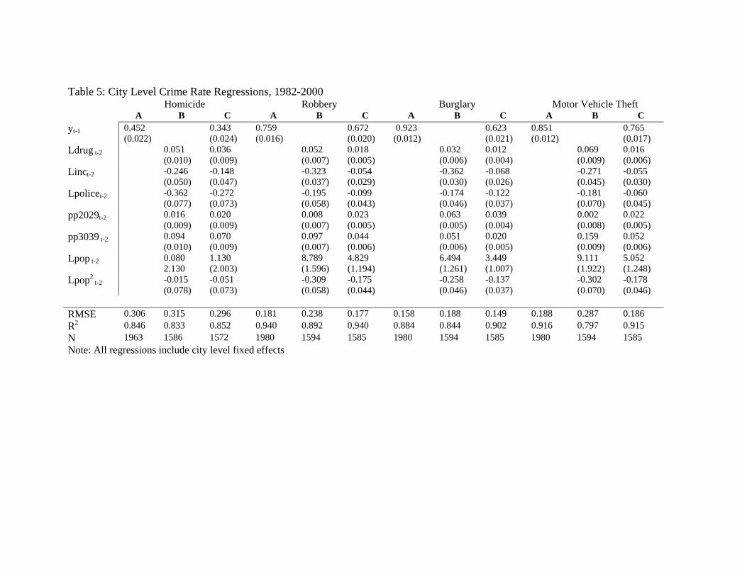
Table 5: City Level Crime Rate Regressions, 1982-2000 Homicide Robbery Burglary Motor Vehicle Theft A B C A B C A B C A B C yt-1 0.452

(0.022) 0.343

(0.024) 0.759 (0.016)

0.672 (0.020)

0.923 (0.012)

0.623 (0.021)

0.851 (0.012)

0.765 (0.017)

Ldrug t-2 0.051 (0.010)

0.036 (0.009)

0.052 (0.007)

0.018 (0.005)

0.032 (0.006)

0.012 (0.004)

0.069 (0.009)

0.016 (0.006)

Linct-2 -0.246 (0.050)

-0.148 (0.047)

-0.323 (0.037)

-0.054 (0.029)

-0.362 (0.030)

-0.068 (0.026)

-0.271 (0.045)

-0.055 (0.030)

Lpolicet-2 -0.362 (0.077)

-0.272 (0.073)

-0.195 (0.058)

-0.099 (0.043)

-0.174 (0.046)

-0.122 (0.037)

-0.181 (0.070)

-0.060 (0.045)

pp2029t-2 0.016 (0.009)

0.020 (0.009)

0.008 (0.007)

0.023 (0.005)

0.063 (0.005)

0.039 (0.004)

0.002 (0.008)

0.022 (0.005)

pp3039 t-2 0.094 (0.010)

0.070 (0.009)

0.097 (0.007)

0.044 (0.006)

0.051 (0.006)

0.020 (0.005)

0.159 (0.009)

0.052 (0.006)

Lpop t-2 0.080 2.130

1.130 (2.003)

8.789 (1.596)

4.829 (1.194)

6.494 (1.261)

3.449 (1.007)

9.111 (1.922)

5.052 (1.248)

Lpop2 t-2 -0.015

(0.078) -0.051 (0.073)

-0.309 (0.058)

-0.175 (0.044)

-0.258 (0.046)

-0.137 (0.037)

-0.302 (0.070)

-0.178 (0.046)

RMSE 0.306 0.315 0.296 0.181 0.238 0.177 0.158 0.188 0.149 0.188 0.287 0.186 R2 0.846 0.833 0.852 0.940 0.892 0.940 0.884 0.844 0.902 0.916 0.797 0.915 N 1963 1586 1572 1980 1594 1585 1980 1594 1585 1980 1594 1585 Note: All regressions include city level fixed effects

Table 6: Summary of 100 City Specific AR(1) Coefficients Homicide Robbery Burglary MVT Heterogeneous Model IQR [0.220,0.751] [0.634, 0.894] [0.832, 1.012] [0.805, 0.919] Median 0.567 0.798 0.963 0.861 Mean 0.486 0.752 0.902 0.822 Minimum -0.585 0.023 0.029 -0.021 Maximum 1.059 1.129 1.371 1.117 Homogeneous Model 0.452 0.759 0.923 0.851

Table 7: Heterogeneous Model Coefficient Estimates for Selected Cities Homicide Robbery Burglary MVT Denver 0.63 0.94 1.02 0.68 Knoxville -0.03 0.76 1.01 0.73 Madison 0.25 0.65 0.95 0.93 New York 1.06 1.13 1.07 1.12 Richmond 0.76 0.73 0.90 0.67 San Francisco 0.73 0.94 0.94 0.95

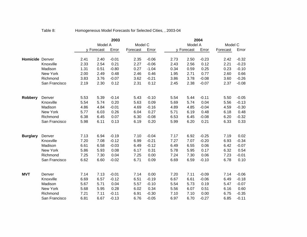
Table 8: Homogeneous Model Forecasts for Selected Cities, , 2003-04

y Forecast Error Forecast Error y Forecast Error Forecast Error

Homicide Denver 2.41 2.40 -0.01 2.35 -0.06 2.73 2.50 -0.23 2.42 -0.32Knoxville 2.33 2.54 0.21 2.27 -0.06 2.43 2.56 0.12 2.21 -0.23Madison 1.31 0.51 -0.80 0.27 -1.04 0.34 0.59 0.25 0.23 -0.10New York 2.00 2.49 0.48 2.46 0.46 1.95 2.71 0.77 2.60 0.66Richmond 3.83 3.76 -0.07 3.62 -0.21 3.86 3.78 -0.08 3.60 -0.26San Francisco 2.19 2.30 0.12 2.31 0.12 2.45 2.38 -0.07 2.37 -0.08

Robbery Denver 5.53 5.39 -0.14 5.43 -0.10 5.54 5.44 -0.11 5.50 -0.05Knoxville 5.54 5.74 0.20 5.63 0.09 5.69 5.74 0.04 5.56 -0.13Madison 4.86 4.84 -0.01 4.69 -0.16 4.89 4.85 -0.04 4.59 -0.30New York 5.77 6.03 0.26 6.04 0.27 5.71 6.19 0.48 6.18 0.48Richmond 6.38 6.45 0.07 6.30 -0.08 6.53 6.45 -0.08 6.20 -0.32San Francisco 5.98 6.11 0.13 6.19 0.20 5.99 6.20 0.21 6.33 0.33

Burglary Denver 7.13 6.94 -0.19 7.10 -0.04 7.17 6.92 -0.25 7.19 0.02

Knoxville 7.20 7.08 -0.12 6.99 -0.21 7.27 7.07 -0.20 6.93 -0.34Madison 6.61 6.58 -0.03 6.49 -0.12 6.49 6.55 0.06 6.42 -0.07New York 5.86 5.93 0.08 6.17 0.31 5.78 5.95 0.17 6.32 0.54Richmond 7.25 7.30 0.04 7.25 0.00 7.24 7.30 0.06 7.23 -0.01San Francisco 6.62 6.60 -0.02 6.71 0.09 6.69 6.59 -0.10 6.78 0.10

MVT Denver 7.14 7.13 -0.01 7.14 0.00 7.20 7.11 -0.09 7.14 -0.06 Knoxville 6.69 6.57 -0.12 6.51 -0.19 6.67 6.61 -0.06 6.49 -0.18 Madison 5.67 5.71 0.04 5.57 -0.10 5.54 5.73 0.19 5.47 -0.07 New York 5.68 5.95 0.28 6.02 0.34 5.56 6.07 0.51 6.16 0.60 Richmond 7.21 7.11 -0.11 6.91 -0.30 7.10 7.10 0.00 6.75 -0.35 San Francisco 6.81 6.67 -0.13 6.76 -0.05 6.97 6.70 -0.27 6.85 -0.11

Model CModel CModel A2003

Model A2004

Table 9: Homogeneous Model Forecast Error Summary, All Cities, 2003-2004

Model A Model C Naïve_02 Model A Model C Naïve_02

HomicideMean 2.32 2.32 2.32 2.29 2.29 2.29Mean Forecast 2.44 2.16 2.31 2.49 2.16 2.31Mean Error 0.12 -0.09 -0.01 0.20 -0.08 0.02Fraction Positive 0.67 0.36 0.46 0.71 0.36 0.52RMSE 0.37 0.41 0.40 0.37 0.35 0.34Mean Absolute Error 0.25 0.28 0.25 0.30 0.28 0.25

RobberyMean 5.68 5.68 5.68 5.67 5.67 5.67Mean Forecast 5.78 5.59 5.73 5.82 5.58 5.73Mean Error 0.10 -0.004 0.05 0.14 -0.04 0.05Fraction Positive 0.75 0.38 0.59 0.77 0.42 0.59RMSE 0.24 0.25 0.22 0.23 0.22 0.17Mean Absolute Error 0.14 0.14 0.11 0.19 0.18 0.13

BurglaryMean 6.99 6.99 6.99 6.99 6.99 6.99Mean Forecast 7.01 6.90 7.01 7.01 6.87 7.01 Mean Error 0.01 -0.04 0.01 0.01 -0.08 0.02Fraction Positive 0.52 0.35 0.50 0.59 0.29 0.59RMSE 0.18 0.23 0.18 0.13 0.23 0.13Mean Absolute Error 0.09 0.13 0.08 0.10 0.16 0.10

MVTMean 6.69 6.69 6.69 6.66 6.66 6.69Mean Forecast 6.72 6.59 6.71 6.73 6.55 6.71

Mean Error 0.03 -0.06 0.02 0.07 -0.10 0.05 Fraction Positive 0.58 0.43 0.54 0.59 0.29 0.59 RMSE 0.24 0.28 0.23 0.22 0.29 0.20 Mean Absolute Error 0.13 0.18 0.12 0.17 0.24 0.16

Note: Naive(02) is a random walk forecasts where 2002 is treated as the last observed year.

2003 2004

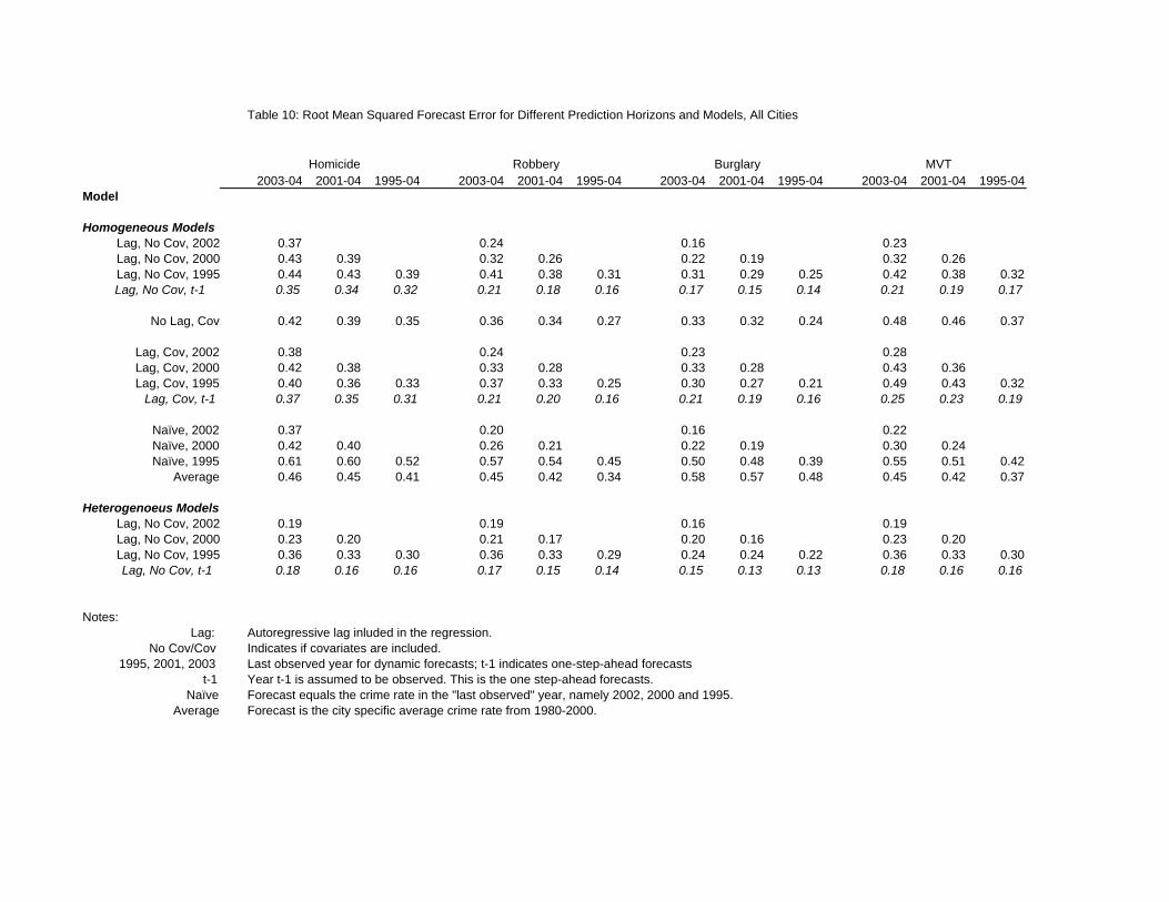
Table 10: Root Mean Squared Forecast Error for Different Prediction Horizons and Models, All Cities

2003-04 2001-04 1995-04 2003-04 2001-04 1995-04 2003-04 2001-04 1995-04 2003-04 2001-04 1995-04

Model

Homogeneous ModelsLag, No Cov, 2002 0.37 0.24 0.16 0.23 Lag, No Cov, 2000 0.43 0.39 0.32 0.26 0.22 0.19 0.32 0.26 Lag, No Cov, 1995 0.44 0.43 0.39 0.41 0.38 0.31 0.31 0.29 0.25 0.42 0.38 0.32Lag, No Cov, t-1 0.35 0.34 0.32 0.21 0.18 0.16 0.17 0.15 0.14 0.21 0.19 0.17

No Lag, Cov 0.42 0.39 0.35 0.36 0.34 0.27 0.33 0.32 0.24 0.48 0.46 0.37

Lag, Cov, 2002 0.38 0.24 0.23 0.28 Lag, Cov, 2000 0.42 0.38 0.33 0.28 0.33 0.28 0.43 0.36 Lag, Cov, 1995 0.40 0.36 0.33 0.37 0.33 0.25 0.30 0.27 0.21 0.49 0.43 0.32

Lag, Cov, t-1 0.37 0.35 0.31 0.21 0.20 0.16 0.21 0.19 0.16 0.25 0.23 0.19

Naïve, 2002 0.37 0.20 0.16 0.22 Naïve, 2000 0.42 0.40 0.26 0.21 0.22 0.19 0.30 0.24 Naïve, 1995 0.61 0.60 0.52 0.57 0.54 0.45 0.50 0.48 0.39 0.55 0.51 0.42

Average 0.46 0.45 0.41 0.45 0.42 0.34 0.58 0.57 0.48 0.45 0.42 0.37

Heterogenoeus ModelsLag, No Cov, 2002 0.19 0.19 0.16 0.19 Lag, No Cov, 2000 0.23 0.20 0.21 0.17 0.20 0.16 0.23 0.20 Lag, No Cov, 1995 0.36 0.33 0.30 0.36 0.33 0.29 0.24 0.24 0.22 0.36 0.33 0.30Lag, No Cov, t-1 0.18 0.16 0.16 0.17 0.15 0.14 0.15 0.13 0.13 0.18 0.16 0.16

Notes:Lag: Autoregressive lag inluded in the regression.

No Cov/Cov Indicates if covariates are included.1995, 2001, 2003 Last observed year for dynamic forecasts; t-1 indicates one-step-ahead forecasts

t-1 Year t-1 is assumed to be observed. This is the one step-ahead forecasts.Naïve Forecast equals the crime rate in the "last observed" year, namely 2002, 2000 and 1995.

Average Forecast is the city specific average crime rate from 1980-2000.

Homicide Robbery Burglary MVT

Table 11: Homogeneous Model Forecasts for Selected Cities, , 2005-2009

2004 2009 Model

A C A C A 2009-2004

Homicide Denver 2.73 2.65 2.55 2.61 2.47 2.59 -0.15Knoxville 2.43 2.51 2.25 2.54 2.20 2.56 0.13Madison 0.34 0.51 0.25 0.59 0.22 0.64 0.31New York 1.95 2.47 . 2.70 . 2.88 0.93Richmond 3.86 3.82 3.66 3.81 3.58 3.79 -0.06San Francisco 2.45 2.45 2.41 2.45 2.40 2.45 -0.01

Robbery Denver 5.54 5.55 5.58 5.56 5.59 5.58 0.03Knoxville 5.69 5.70 5.60 5.71 5.54 5.72 0.02Madison 4.89 4.88 4.72 4.88 4.60 4.87 -0.02New York 5.71 5.94 . 6.12 . 6.44 0.73Richmond 6.53 6.51 6.35 6.49 6.22 6.47 -0.06San Francisco 5.99 6.11 6.19 6.20 6.32 6.37 0.38

Burglary Denver 7.17 7.14 7.23 7.11 7.27 7.03 -0.14Knoxville 7.27 7.24 7.10 7.21 6.99 7.14 -0.12Madison 6.49 6.47 6.41 6.45 6.36 6.41 -0.08New York 5.78 5.80 . 5.82 . 5.88 0.11Richmond 7.24 7.24 7.21 7.25 7.19 7.26 0.02San Francisco 6.69 6.67 6.76 6.66 6.81 6.62 -0.07

MVT Denver 7.20 7.17 7.18 7.14 7.15 7.09 -0.11 Knoxville 6.67 6.69 6.61 6.71 6.57 6.75 0.08 Madison 5.54 5.58 5.44 5.61 5.37 5.69 0.15 New York 5.56 5.74 . 5.89 . 6.22 0.66 Richmond 7.10 7.09 6.89 7.08 6.73 7.06 -0.03 San Francisco 6.97 6.95 7.01 6.93 7.03 6.90 -0.07

Model Model2005 2006

Table 12: Homogeneous Model Forecasts Summary, All Cities, 2005-2009

2009

2004 Model A Model C Model A Model C Model A

HomicideMean Forecast 2.29 2.42 2.17 2.49 2.14 2.53Mean Change from 2004 0.14 -0.07 0.20 -0.10 0.24Fraction Positive Change 0.75 0.35 0.75 0.34 0.75IQR [0.01,0.26] [-0.23,0.07] [0.01, 0.37] [-0.30, 0.10] [0.01, 0.46]Mean Abosolute Change 0.19 0.20 0.27 0.27 0.33

RobberyMean Forecast 5.67 5.73 5.57 5.78 5.54 5.87Mean Change from 2004 0.06 -0.04 0.11 -0.07 0.20Fraction Positive Change 0.82 0.350 0.82 0.36 0.82IQR [0.01, 0.12] [-0.12,0.01] [0.02, 0.21] [-0.20, 0.02] [0.04,0.37]Mean Abosolute Change 0.08 0.09 0.13 0.15 0.23

BurglaryMean Forecast 6.99 6.99 6.91 6.99 6.88 6.99Mean Change from 2004 0.00 -0.06 0.00 -0.09 0.00Fraction Positive Change 0.54 0.28 0.54 0.28 0.54IQR [-0.01, 0.01] [-0.10, 0.01] [-.0.02, 0.02] [-0.18,0.01] [-.0.04, 0.05]Mean Abosolute Change 0.01 0.09 0.03 0.15 0.06

MVTMean Forecast 6.66 6.68 6.59 6.70 6.52 6.74Mean Change from 2004 0.02 -0.08 0.03 -0.14 0.07

Fraction Positive Change 0.68 0.19 0.68 0.17 0.68 IQR [-0.02, 0.05] [-0.14, -0.03] [-0.04, 0.10] [-0.25,-0.05] [-0.08,0.20] Mean Abosolute Change 0.05 0.11 0.09 0.20 0.18

2005 2006