forecasting and analyzing world commodity prices - … · forecasting and analyzing world commodity...
TRANSCRIPT
t
onentsricesaper,ove-
CNEerror-thesels’ per-of theU.S.realorld
mpo-real
gres-(f) ase of
______rla-
. Spe-n thisda.
Forecasting and Analyzing World Commodity Prices
René Lalonde* Zhenhua Zhu Frédérick Demers** Principal Researcher Economist Economist International Department Research Department Research Departmen Bank of Canada Bank of Canada Bank of Canada
October 18, 2002
Abstract
This paper develops simple econometric models to analyze and forecast three compof the Bank of Canada commodity price index (BCPI), namely non-energy commodity p(BCNE), the West Texas Intermediate crude oil price (WTI), and other energy prices. In the pwe present different methodologies to identify transitory and permanent components of mments in these prices. A structural vector autoregressive (SVAR) model is used for real Bprices, a multiple structural-break technique is employed for real crude oil prices, and ancorrection model is constructed for real prices of other energy components. Then we usetransitory and permanent components to develop forecasting models. We assess our modeformance in various aspects, and our main results indicate: (a) for real BCNE prices, mostshort-run variation is attributed to demand shocks, (b) the world economic activity and realdollar effective exchange rate explain much of the cyclical variation of real BCNE prices, (c)crude oil prices have two structural breaks over the sample period, and their link with the weconomic activity is strongest in the most recent regime, (d) real prices of other energy conents are highly correlated with the U.S. economic activity, and they are co-integrated withcrude oil prices, (e) our models outperform benchmark models, namely a VAR model, autoresive (AR) model and a random walk (RW) model, in terms of out-of-sample forecasting, and1% positive shock to world economic activity leads to an approximate 7.2% peak responworld commodity prices.
________________________________________________________________________* Corresponding author. Contact address: 234 Wellington St. Ottawa, ON, K1A 0G9. E-mail:[email protected]** The authors would like to thank seminar participants at the Bank of Canada for useful commentscial thanks also to Donald Coletti, Allan Crawford and Simon van Norden. The views expressed ipaper are those of the authors. No responsibility for them should be attributed to the Bank of Cana
0
omy,
repre-
s have
e real
Price
xed-
d sold
od-
d by
non-
ergy
or.
ices.
model
n of
rices,
ingle
BCNE
run.
f real
all but
d
d.
rate
1. Introduction
The resource sector has traditionally played an important role in the Canadian econ
especially in the area of foreign trade. Over the past decade, total exports of commodities
sent, on average, about forty one per cent of Canada's exports of goods1 and fifteen per cent of
Canada's gross domestic product (GDP). Consequently, changes in world commodity price
historically been a key determinant of Canada's terms of trade, which in turn have affected th
income of Canadians.
The staff at the Bank of Canada (BOC) have designed the Bank of Canada Commodity
Index (BCPI) to track the prices paid for key Canadian commodities. The BCPI is a fi
weighted index of the spot or transaction prices of 23 commodities produced in Canada an
in world markets.2 All components of the BCPI are priced in U.S. dollars. The choice of comm
ities is determined by their importance in Canadian production, subject to limitations impose
data availability. For the purpose of this paper, we split the BCPI into three subindices:
energy commodity prices (BCNE), the West Texas Intermediate crude oil price (WTI), and en
prices excluding crude oil.3 To obtain real commodity prices, we divide by the U.S. GDP deflat
In this paper, we employ three different empirical approaches to model commodity pr
For real BCNE prices, we use an approach that combines a structural vector autoregressive
(SVAR) with a single equation model. The SVAR is used to give us a historical decompositio
movements in real BCNE prices, and to project the permanent (or long-run) component of p
while the transitory (or short-run) component of real BCNE prices is forecasted with a s
equation model. We find that this approach successfully captures the strong linkage of real
prices with the world economic activity and the real U.S. effective exchange rate in the short4
A 1% positive shock to world economic activity leads to an approximate 6% peak response o
BCNE prices, while the response to the real U.S. dollar effective exchange rate shock is sm
1. This ratio is defined as the share of nominal commodity exports in total nominal exports over the perio1990 to 2001.
2. See Appendix A for a description of the BCPI and its components. The weight of each commodity in theindex is based on the average value of Canadian production of the commodity over the 1982-90 perio
3. The other energy price index consists of natural gas prices (80%) and coal prices (20%).4. The U.S. dollar effective exchange rate is defined as a U.S. export weighted average of the exchange
of U.S. dollar relative to the currencies of Japan (17.59%), U.K. (8.22%), Mexico (14.52%), Canada(35.40%) and Euro zone (24.27%)
1
NE
s.
egres-
or real
cant
for
hock
rices
odel
com-
nship
gap, a
hort-
eco-
ight is
total,
nse of
ecent
or the
e dis-
is
can-
it is statistically significant and exhibits the expected sign.5 We also find that the variance of the
transitory component of real BCNE prices accounts for approximately 60% of total real BC
price variance. This result is consistent with numerous other studies of commodity price6 In
terms of out-of-sample forecasting, our approach outperforms a SVAR model and an autor
sive (AR) model.
Two separate models are used for real crude oil prices and other real energy prices. F
crude oil prices, we use a statistical multiple structural-break approach to identify signifi
shifts in OPEC behavior. After controlling for these mean shifts, we find a very strong role
world economic activity in the determination of oil prices. We estimate that a 1% positive s
to world economic activity leads to an approximate 12% peak response of real crude oil p
with a lag of two to three quarters. In terms of out-of-sample forecasts, the real oil price m
outperforms an AR model and a random walk (RW) model. For real prices of other energy
ponents, we use an error correction representation which exploits the long-run relatio
between real energy prices excluding crude oil and real crude oil prices. The U.S. output
proxy for North American economic conditions, is shown to be a key factor explaining the s
run price variations.7
To quantify the total peak response of the total BCPI to a 1% positive shock to world
nomic activity, we take the weighted sum of three component responses, where the we
determined by the share of each individual component in the composition of the BCPI. In
we estimate that a 1% positive shock to world economic activity leads to a 7.2% peak respo
world commodity prices. This is close to the result reported in Hunt (1995).
The remainder of the paper is organized as follows. Section 2 gives a brief overview of r
literature on commodity prices. In Section 3, we present the methodology as well as results f
real BCNE price model. The methodologies and results for the real crude oil price model ar
5. We use the world output gap as a proxy for the overall world economic activity, where the output gapgenerated using the Hodrick-Prescott (HP) filter.
6. For example, Borensztein and Reinhart (1994) obtain a similar result.7. Due to the difficulty and cost associated with transportation of natural gas overseas, natural gas prices
be thought of as determined in North American markets while crude oil prices are more globally determined.
2
crude
ction
g to
been
ment.
run.
world
hes,
e first
-series
ach of
can eas-
ntals.
very
state
ee that
state
the
dopt
por-
side,
cle in
. On
con-
cussed in Section 4. Section 5 presents results for the model of real energy prices excluding
oil. Section 6 reports the peak response of the BCPI to a shock to world economic activity. Se
7 concludes.
2. Literature Review
This section gives a brief overview of some of the recent economic literature pertainin
price formation in world commodity markets. A common theme in many of these studies has
an attempt to disentangle commodity price movements into a cyclical and a long-term move
This distinction is important for forecasting commodity prices both in the short-run and long-
Various methodologies have been used in order to disentangle the trend movement of
commodity prices from the cycle. Reinhart and Wickham (1994) apply two different approac
namely the Beveridge and Nelson (1981) technique and the Harvey (1985) approach. Th
approach is a pure reduced form time-series technique used for the decomposition of a time
variable, while the second one is a structural time-series approach using the Kalman filter. E
these two approaches has its own strengths and weaknesses. The pure mechanical filters
ily split a time series into cyclical and permanent components, but lack economic fundame
Although the Kalman filter contains certain economic information, it often does not perform
well in practice if the assumptions of normal distributions for disturbances and the initial
vector are violated. When the normality assumption is dropped, there is no longer a guarant
the Kalman filter will give the conditional mean of the state vector, i.e. the estimates of the
vector could be conditionally biased.8 Moreover, it becomes more cumbersome to calculate
likelihood function without the normality assumption.
Following the study of Reinhart and Wickham (1994), Borensztein and Reinhart (1994) a
a structural model to identify the key fundamentals behind commodity prices, and more im
tantly to quantify the relative contributions of demand and supply shocks. On the demand
they find that the real U.S. dollar effective exchange rate and the state of the business cy
industrial countries are closely linked to the cyclical movement of world commodity prices
the supply side, strong productivity growth of commodity sectors relative to the rest of the e
8. See Harvey (1989) for details.
3
imary
uthors
near
odity
tead of
odity
high
ow-
o the
exam-
at the
lity of
odity
t there
ause of
ns.
d per-
s suf-
ls are
evelop
ivid-
series
r BOC
ne
omy and the increased commodity supply relative to the rest of the economy are the pr
causes of the downward trend of commodity prices. Using a variance decomposition, the a
conclude that both types of shocks contribute to the total variation of commodity prices in the
term and around 60% of the variation is caused by demand shocks.
Cashin, Liang and McDermott (2000) examine the persistence of shocks to comm
prices. They use a median-unbiased estimation procedure proposed by Andrews (1993) ins
a unit root test to check the persistence of shocks. Using IMF data on sixty individual comm
prices, they find that shocks to most commodity prices are long-lasting (reflected by the
value of the half-life of a unit shock), and the variability of the persistence is fairly large. H
ever, they fail to identify and quantify the relative importance of demand and supply factors t
persistence of shocks. Cashin and McDermott (2001) use much longer sample periods and
ine whether the long-run behavior of commodity prices has changed. In particular, they look
trend of most commodity prices, the duration of price booms and slumps, and also the volati
price movements. They apply various statistical tests and compare the patterns of comm
price movements across different sample periods. The authors come to the conclusion tha
has been an apparent downward trend in real commodity prices over the last 140 years bec
relative productivity growth in commodity sectors and a structural change in supply conditio9
Moreover, the short-term volatility is highly related to the business cycle.
In practice, numerous methodologies have been employed to disentangle transitory an
manent movements in commodity prices. Though convenient to apply, pure time-series filter
fer from a lack of structural economic fundamentals. In contrast, although structural mode
constructed based on the economic theory, they are often costly and time-consuming to d
and maintain. For instance, it would be very costly to develop and maintain models for 23 ind
ual components of the BCPI. Therefore, as a compromise, we combine basic time
approaches with simple economic theory to develop econometric models for the three majo
commodity price indexes.
9. Coletti (1992) examines a small set of non-energy commodities that mainly include industrial materials(e.g. metals, minerals and forest products) over the 1900-91 period. He finds no obvious secular decliin relative prices of those commodities.
4
y used
e last
rma-
on the
that
ed to
an be
onents,
SVAR
f vari-
in the
o-inte-
vious
from
eco-
re
.
two
world
onent
he-m
-m
3. The real BCNE price model
This section consists of three subsections. The first two parts describe the methodolog
to identify and to forecast the transitory and permanent components of real BCNE prices. Th
subsection shows the results.
3.1 Identifying the transitory and permanent components of real BCNE prices
We use a SVAR approach to decompose historical BCNE prices into transitory and pe
nent components. Under this approach, a number of economic restrictions are imposed
long-run effects of different types of shocks. The main strength of the SVAR methodology is
one does not have to impose a fully specified theoretical structure and the data are allow
speak. The only assumptions are that the variable of interest (i.e. real BCNE prices) c
decomposed into one or more permanent components and one or more transitory comp
and that the transitory shocks are uncorrelated with the permanent shocks. However, the
methodology has its own weakness. Notably, the results are often sensitive to the choice o
ables included in the estimation. Also, results can be affected by the number of lags chosen
reduced form, assumptions on the order of integration of variables, and the presence of c
grating relationships among variables.
In our model, variable selection is based on economic theory and the findings of pre
studies. To capture the information about transitory shifts in real BCNE prices arising
changes in world economic conditions, we use the G7 output gap as a proxy for the world
nomic activity.10 The G7 inflation rate,11 a proxy for the global inflation rate, is added to captu
the importance of having a nominal anchor in the model as suggested by the SVAR literature12 In
light of the empirical studies on world commodity prices in the previous section, we include
additional demand indicators - the real U.S. long-term interest rate as a proxy for the real
interest rate, and the real U.S. dollar effective exchange rate - to identify the cyclical comp
10.The G7 output gap is generated using the SVAR methodology for the U.S. (see Lalonde (1998)) and tHP filter for the rest of G7 countries. We take the sum of individual output gaps weighted by each country's share in the composition of the G7 output evaluated at purchasing power parity. We use the ter“world output gap” through the rest of the paper.
11.The G7 inflation rate is generated by taking the sum of individual inflation rates weighted by each country's share in the composition of the G7 output evaluated at purchasing power parity. We use the ter“global inflation rate” through the rest of the paper.
5
ants
CNE
ta-
st of
s that
1972-
of both
ections
f real
ent of
f real
ndseryelE
l
in
ofust
eal
of real BCNE prices.13 In addition, we have attempted to include some supply-side determin
of the permanent component of real BCNE prices. However, given the fact that the real B
price is an aggregate price index, it is hard to find a proper measure of productivity.14
The final SVAR contains the following five variables: real BCNE prices (Rbcne), the world
output gap (Wygap), the global inflation rate (Wπ), the real U.S. long term interest rate (RRus) and
the real U.S. dollar effective exchange rate (Erus). We assume that the real U.S. interest rate is s
tionary in levels.15 ADF tests show that the world output gap is stationary in levels and the re
variables are first difference stationary. Furthermore, a Johansen co-integration test show
there is no co-integrating relationship betweenRbcne, Wπ andErus. The technical details on the
SVAR methodology are presented in Appendix B. We estimate the model over the period of
2001 using quarterly data.16
3.2 Forecasting the transitory and permanent component of real BCNE prices
The second step of the approach consists of finding the best way to produce forecasts
the temporary and permanent components that are both tractable and consistent with proj
of the rest of the world economy. We use the SVAR to forecast the permanent component o
BCNE prices. We have also estimated a simple equation to forecast the transitory compon
real BCNE prices. This equation captures the link between the transitory component o
BCNE prices and the world output gap as well as the real U.S. effective exchange rate gap.17 The
12.If monetary policy has a neutral effect across different sectors of the economy, both in the short-run along run, the presence of the global inflation rate in the model may not be important. However, becaumonetary policy may not affect all sectors in the same manner in the short-run, it can have a transitoeffect on relative prices. Consequently, using real BCNE prices alone may not be sufficient to purge theffects of monetary policy. Out-of-sample forecasting performance of the model including the globainflation rate is slightly better than the one which excludes it. Furthermore, results show that real BCNprices do react, in the short-run, to a shock affecting the trend inflation rate.
13.Since world commodities are all priced in U.S. dollars, movements in the real U.S. dollar effectiveexchange rate will affect the demand for commodities by countries other than the U.S. This in turn wilaffect prices.
14.If the productivity growth only happens in a particular sector, this tends to lower production cost in thissector relative to the rest of the economy. Consequently, this causes lower prices of goods producedthis sector relative to the aggregate level (i.e. lower relative prices).
15.The augmented Dickey-Fuller (ADF) test provides an ambiguous evidence regarding the stationaritythe real U.S. long-term interest rate. However, we assume here that it is stationary. The results are robto this assumption.
16.We estimate the same model over the sample of 1972-95 and we find that the transitory component of rBCNE prices is almost identical to the one estimated over the full sample period.
6
the
small
n addi-
ange
mpo-
ss the
last
ons.
of the
and
ficant
t with
BCNE
es
supply
g
equation is defined as:
Regression Equation:
Rbcnegapt = A(L)Rbcnegapt-1 + B(L)Wygapt + C(L)Ergapt ,18 (1)
whereRbcnegapis the transitory component of real BCNE prices (i.e. real BCNE price minus
SVAR estimates of its permanent component),Wygapis the world output gap andErgap is the
real U.S. dollar effective exchange rate gap. This equation has the advantage of relying on a
number of estimated parameters, which helps to reduce out-of-sample forecasting errors. I
tion, it clearly quantifies the impacts of the world output gap and the real U.S. dollar exch
rate gap on the change in the transitory component of real BCNE prices.
3.3 Results of real BCNE price model
This section presents results of the real BCNE price model. First, we use variance deco
sition to quantify the relative importance of supply and demand shocks. Second, we discu
link between the world output gap and the transitory component of real BCNE prices. The
part evaluates the forecasting performance of the model.
3.3.1 The relative importance of supply and demand shocks
Table 1 reports the variance decomposition of real BCNE prices at different time horiz
After the first year (step=4), the transitory shocks (i.e. demand shocks) explain almost 60%
total variance of real BCNE prices. After two years (step=8), however, the contribution of dem
shocks falls dramatically and accounts for only 10% of the total. The model shows a signi
contribution of demand shocks to real BCNE prices in the short term, and this is consisten
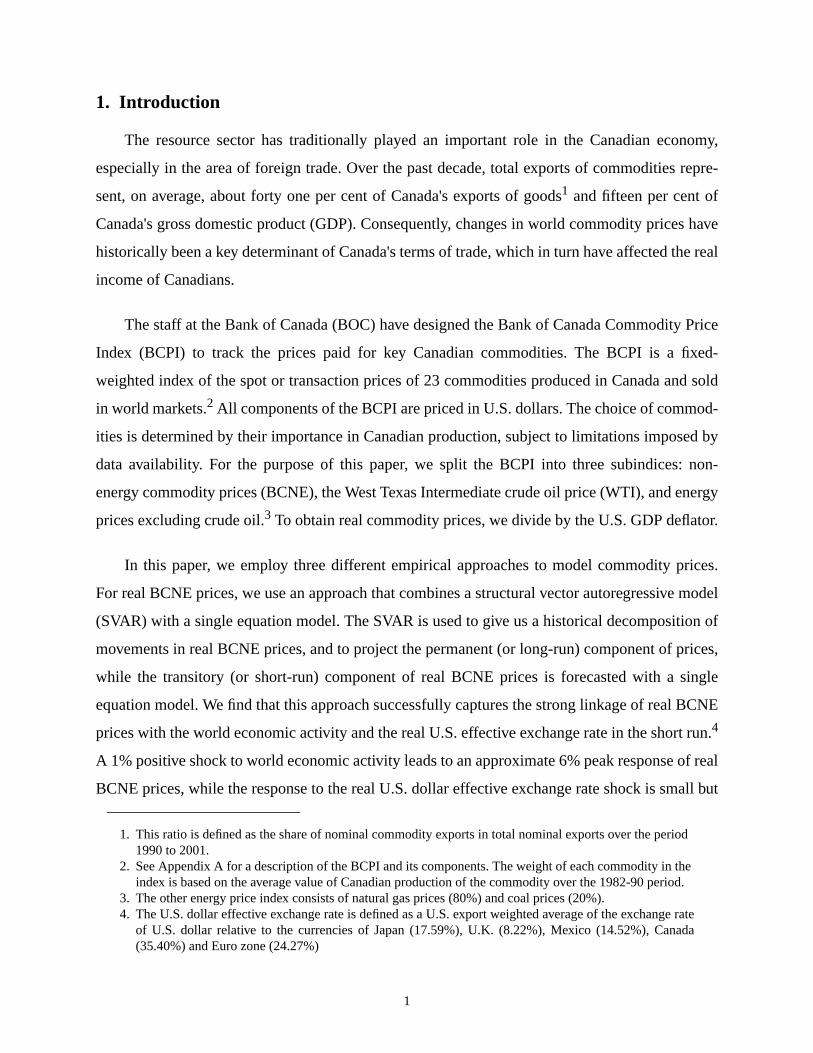
other studies mentioned earlier. Figure 1 plots the corresponding impulse responses of real
prices to a positive one standard deviationtotal demand and supply shock. Real BCNE pric
exhibit a small hump-shaped response to the total demand shock while the response to the
shock appears to be more gradual.
17.We use the HP filter to generate the real U.S. dollar exchange rate gap.18.It is worth noting here that the real U.S. interest rate is excluded in the equation due primarily to its stron
collinearity with the world output gap, but it can still indirectly affect the forecast of real BCNE prices viaits impact on the forecast of the world output gap.
7
f real
e two
CNE
ect the
riable
gap,
e real
using
ve the
sig-
nd are
lf is
ollar
rices.
ock to
e find
nd the
f the
plied
and 5
nd the
prices
eak of
apre
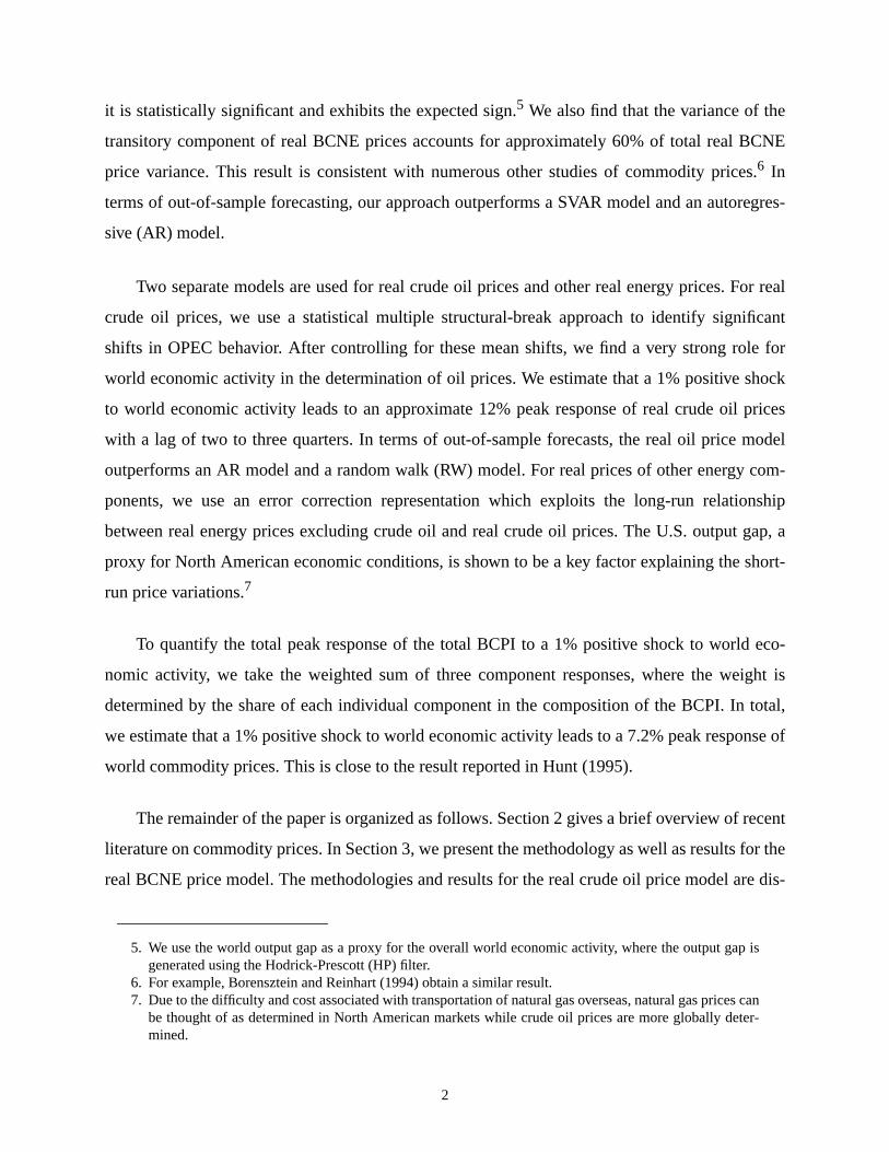
3.3.2 The world output gap and the transitory component of real BCNEprices19
Figure 2 plots the evolution of both the world output gap and the transitory component o
BCNE prices over the historical period. There is a strong positive relationship between th
variables. The world output gap tracks most of the important cyclical movements of real B
prices since the mid 1970s.
Table 2 reports the parameter estimates of equation (1). The Hausman test fails to rej
null hypothesis of exogeneity of the world output gap, and hence we use instrumental va
estimation (IVE). The instruments used for the estimation are four lags of the world output
the transitory component of real BCNE prices, the real U.S. dollar exchange rate gap and th
U.S. long-term interest rate. The standard errors of the estimated parameters are modified
an 8-lag Newey-West correction. We start with eight lags for each regressor, and then remo
most insignificant estimates one by one until all the remaining coefficients are statistically
nificant at the 5% significance level. All the coefficient estimates have the expected signs a
statistically significant in the final model. The transitory component of real BCNE prices itse
fairly persistent with a root of about 0.71, and both the world output gap and the real U.S. d
effective exchange rate gap contribute significantly to transitory movements of real BCNE p
Furthermore, we calculate the relative contributions of a positive one standard deviation sh
each regressor in our model to the total response of the real BCNE transitory component. W
that around 80% of the total response comes from shocks to the world output gap (72%) a
real U.S. dollar exchange rate gap (8%). In other words, only a small fraction (20%) o
response is left unexplained by our model.
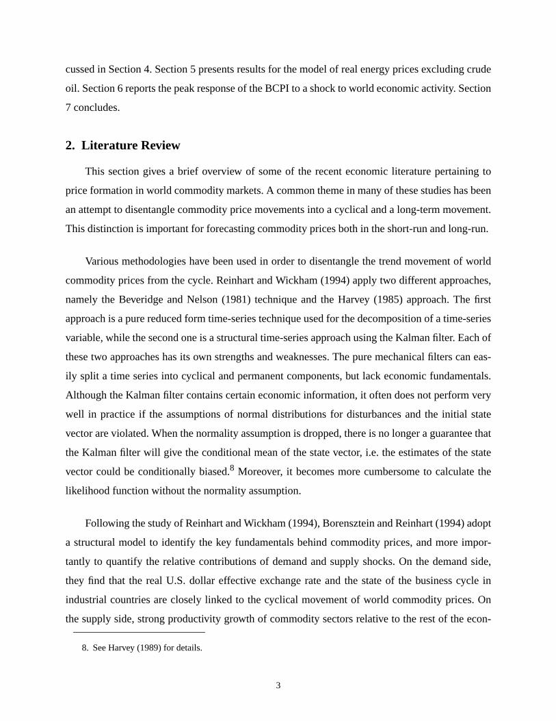
Figure 3 plots the real BCNE price versus its permanent component over history. The im
cyclical movements of real BCNE prices are consistent with our expectations. Figures 4
show the responses of real BCNE prices to a 1% positive shock to the world output gap a
real U.S. dollar effective exchange rate gap respectively. The peak response of real BCNE
to the world output gap shock is about 6% and occurs almost contemporaneously with the p
19.As a robustness checking, we also try the U.S. output gap. We find that models with the world output goutperform those with the U.S. output gap in most cases. All results for the U.S. output gap model aavailable upon request.
8
ective
sign.
f two
Since
the
four
fore-
f real
ecasts
ich is
MSE
-
ding to
rigi-
e out-
bined
es B”,
y to
sting
gty
is
s to
the world output gap itself. In comparison, the response to a shock to the real U.S. dollar eff
exchange rate gap is much smaller, with a peak of about -0.35%, but it exhibits the expected
3.3.3 Out-of-sample forecast of real BCNE prices
World commodity price shocks have a peak impact on the core inflation rate with a lag o
to four quarters in the Canadian economic projection model used at the Bank of Canada.
monetary policy tends to have its full impact on inflation with a lag of six to eight quarters,
monetary authority will be most interested in forecasts of world commodity prices two to
quarters ahead.
We evaluate our model's out-of-sample forecasting performance by comparing it with
casts from two benchmark models: VAR model and AR(1) model. Our model forecasts o
BCNE prices combine SVAR forecasts of the permanent component and single equation for
of the transitory component. As mentioned earlier, we focus on the forecasting horizon wh
of interest to the monetary authority, namely two to four-quarters ahead. According to the R
of out-of-sample forecasts from 1992q1 to 2001q4,20 the combined approach uniformly outper
forms the two benchmark models regardless of the forecasting horizons (see Table 3) accor
smaller values of RMSE.21
Tables 4 to 6 report thep-values of the forecast encompassing test statistic, which was o
nally devised by Chong and Hendry (1986) to compare two competing models based on th
of-sample forecasting errors. The encompassing test results support the use of the com
approach. The results indicate that we can not reject the null hypothesis of “A encompass
which implies that forecasts from either of two benchmark models (model B) are unlikel
improve the forecasting performance of the combined approach (model A) for any foreca
20.We use a rolling sample regression to generate out-of-sample forecasts for a given time horizon.21.The fact that the combined approach outperforms the VAR model could be explained by the followin
arguments. The choice of the variables included in the SVAR were not made on the basis of their abilito forecast real BCNE prices but on their ability to give information pertinent to the identification of thepermanent and transitory components of real BCNE prices. Second, SVAR literature shows that itimportant to include a large number of lags in the SVAR in order to identify properly the transitory com-ponent of a variable. With a small sample, this strategy is clearly not optimal in terms of out-of-sampleforecast performance because it relies on many estimated parameters. The combined model attemptaddress those issues.
9
at the
ith the
ce of
e use
rices.
bly in
t the
Perron
and
cross
re the
odel
anent
per-
an-
th
horizon. On the other hand, we can always reject the null hypothesis of “B encompasses A”
5% significance level except for one case when we compare four-quarter ahead forecasts w
RW model. This implies that our combined approach improves the forecasting performan
two benchmark models.
4. The real crude oil price model
This section consists of two subsections. The first part describes the methodology that w
to identify and forecast the transitory and permanent components of real WTI crude oil p
The second subsection presents results of the model.
4.1 Methodologies
Crude oil prices have experienced a few large permanent shifts over history, most nota
1979-80 and 1985-86.22 To test for structural breaks in the data (under the assumption tha
time and the number of breaks is unknown), we use the methodology proposed by Bai and
(1998) (hereafter BP).23 The strength of the BP methodology is that we can estimate the time
the number of structural breaks endogenously with allowance for varying parameters a
regimes. Given the fact that world oil prices are spot prices, we also allow the model to captu
contemporaneous effect of the world output gap on prices.
4.2 Results of the real crude oil price model
This section is divided into three parts. First, we examine the estimation results for the m
of real crude oil prices. Second, we use the estimated model to identify transitory and perm
components of crude oil prices. Third, we evaluate the model's out-of-sample forecasting
formance.
4.2.1 Estimation of real WTI crude oil model
We first consider the real WTI crude oil price over the full sample period. An ADF test c
22.These large movements in price are related to specific developments in the market, particularly wichanges in the behaviour of the OPEC cartel.
23.See Appendix C for a brief discussion of the BP methodology.
10
e can
ce for
work,
level,
s
in the
volu-
e war
mid-
effi-
d with-
almost
0.67
ith the
statis-
rying
across
ses.eis
not reject the presence of a unit root. However, when allowing for structural changes, w
reject the hypothesis that the real WTI crude oil price has a unit root.24
Using the procedure proposed by BP, we estimate a single equation model with allowan
up to three structural changes. The sample period is from 1974q2 to 2001q4. In this frame
all the parameters of the model are allowed to shift at the structural break point. At the 5%
the test is detecting two breaks in 1979q3 and 1985q4.25 It is interesting to note that the test i
capturing the break points matching well the two historical oil price shocks that happened
late 1970s and the mid-1980s. The first oil shock in the late 1970s began with the Iranian re
tion and the accompanying disruption of its petroleum exports. Moreover, the outbreak of th
between Iran and Iraq in 1980 shook the oil market as well. The second oil shock in the
1980s was primarily caused by the collapse of the OPEL cartel.26 The first experiment we do is to
use three dummy variables to capture regimes separated by two breaks.
Regression Equation:
Rwtit = D1* Dumm1 + D2*Dumm2 + D3*Dumm3 + C(L)Rwtit-1 + DD(L)Wygapt + E(L)Ergapt.
Table 7 reports the OLS estimation results of equation (2) without allowing varying co
cients across regimes. We report the model parameter estimates for the two cases with an
out the real U.S. dollar exchange rate gap. As seen in Table 7, the results for both cases are
identical. Real crude oil prices are fairly persistent over the full sample with an AR root of
(the sum of the two autoregressive coefficients) and the estimated coefficient associated w
lagged world output gap is about 2%. The real U.S. dollar effective exchange rate gap is not
tically significant over the whole sample period.
Tables 8 to 10 report the BP procedure results for three regimes with allowance for va
coefficients. As seen, the estimate of the lagged world output gap changes considerably
24.The sum of AR coefficients is 0.58 and thet-statistic is -5.3, which compares to a 2.5% critical value of -5.3 (see Zivotet al (1992)).25.The test statistics for the supF(1|0) and supF(2|1) are 30.7 and 27.4, respectively. This compares to the
5% critical values of 20.1 and 22.1.26.From 1982 to 1985, OPEC attempted to set production quotas low enough to stabilize prices. The
attempts met with repeated failure as various members of OPEC would produce beyond their quotaDuring most of this period, Saudi Arabia acted as the swing producer cutting its production to stem thfree falling prices. In the late 1985, Saudi Arabia stopped doing that and increased its production, and theventually caused the collapse of OPEC and oil price plunge in 1986.
(2)
11
rrect
on-
t 6%,
.
es to
e null
This
nd we
in the
E to
a-
e,
f
ignif-
In the
ge in
eans
ompo-
vari-
world
lag of
itce
.oil
el
regimes. Although it is not statistically significant in the first regime, the estimate has the co
sign. In the second regime, it exhibits the wrong sign, but it is statistically insignificant. In c
trast, its magnitude increases substantially in the most recent regime with a value of abou
which is almost three times the average value over the entire sample as reported in Table 727
Furthermore, since WTI crude oil prices are spot prices, we would expect crude oil pric
respond immediately to the world output gap shock. The Hausman test indicates that th
hypothesis of exogeneity of the world output gap is rejected at 5% level of significance.
implies that applying the OLS to the BP procedure cannot produce consistent estimates, a
should instead use the IVE. The instruments used are four lags of all explanatory variables
model. However, given the small number of observations in the first two regimes, applying IV
the BP procedure tends to give us very biased results.28 Hence, we use IVE to re-estimate equ
tion (2) with an additional variable for world inventories of crude oil only for the third regim
which has a relatively sufficient number of observations.29 Table 11 reports the IVE estimates o
all the parameters. The world output gap remains statistically significant at the 5% level of s
icance, and the estimated coefficient associated with the world output gap is around 4.5%.
preferred model, we also add the change in crude oil inventories. The third lag of the chan
crude oil inventories is statistically significant and exhibits the expected sign.30
4.2.2 The transitory and permanent components of real crude oil prices
Given the nature of the model, the permanent component consists of three different m
caused by two structural breaks. Figure 6 plots the world output gap versus the transitory c
nent of real WTI crude oil prices across the three regimes. The closest link between the two
ables appears in the most recent regime. Figure 7 shows that a 1% positive shock to the
output gap leads to an approximate 12% peak response of real WTI crude oil prices with a
two to three quarters.
27.However, the real U.S. dollar effective exchange rate gap is not statistically significant, and excludingincreases the magnitude and improves the significance of the estimated elasticity of real crude oil priwith respect to the world output gap.
28.The bias problem becomes severe in a small sample. See Davidson and Mackinnon (1993) for details29.As Tables 8 to 10 have shown that the strongest link between the world output gap and real crude
prices is in the third regime, we are more interested in the IVE estimates for this regime.30.Because only the third lag of the change of crude oil inventory enters our model, we do not need a mod
to forecast this variable in order to forecast real oil prices over very short time horizons.
12
rices.
ench-
head
odel.
tper-
e. We
. Fur-
recasts
ample
initial
sults
esis of
y of
l B)
of “B
seful
n real
at real
pecifi-
se the
de oil
4.2.3 Out-of-sample forecast of the real crude oil price model
We use the estimated single equation model from Table 11 to forecast real crude oil p
We compare the two- to four-step ahead forecasting performance of our model with two b
mark models from 1992q1 to 2001q4. Table 12 compares the RMSE of two to four-step a
out-of-sample forecasts of our model with two benchmark models: AR(1) model and RW m
It is evident that regardless of the forecasting horizons concerned, our model uniformly ou
forms the other two as reflected by smaller values of RMSE.
We have also estimated an alternative specification excluding the oil inventory measur
find models excluding the inventory measure always perform worse than those including it
thermore, for near-term forecasting (two quarters ahead), they are even worse than naive fo
using a RW model. Our results are strong in the sense that the first several periods' out-of-s
forecasts may be severely biased given a much smaller number of observations in the
estimations (1986q1 to 1991q1) compared to the whole sample period.
Tables 13 to 15 report thep-values of forecast encompassing test statistics. The test re
again support the use of our model. The results show that we cannot reject the null hypoth
“A encompasses B”, which implies that it is impossible to improve the forecasting capabilit
our model (model A) with the help of forecasts from either of two benchmark models (mode
for any forecast horizon. On the other hand, we can always reject the null hypothesis
encompasses A” at the 10% significance level, which implies that our model can provide u
information to improve the forecasting performance of two benchmark models.
5. The model of real prices of energy excluding crude oil
Using the Johansen co-integration test, we find a co-integrating relationship betwee
crude oil prices and real prices of energy excluding crude oil. The Hausman test shows th
crude oil prices are weakly exogenous in the model. Therefore, we use an error-correction s
cation. Instead of using the world output gap as a measure of real economic activity, we u
U.S. output gap in this model given that the markets for energy components other than cru
are concentrated in North America.
13
ntion-
d, the
es
ly sig-
g-run
se to
orld
shock.
ated a
output
n real
rature
t gap
truc-
enous
erma-
st link
rs in
el was
to
Regression equation:
DRenert = G(L)DRenert-1 + H(L)USygapt + α(Renert-1 + βRwtit-1 +constant). (3)
Table 16 reports the parameter estimates of equation (3). Several points are worth me
ing. First, the U.S. output gap is strongly correlated with short-term price movements. Secon
speed of adjustment coefficient (α) is relatively small (about 14% of the gap between real pric
of other energy components and the long-run trend is adjusted each quarter), but it is high
nificant at the 1% level. Third, the estimated co-integrating relationship indicates that the lon
elasticity of real prices of other energy components with respect to real crude oil prices is clo
one.
6. Response of the BCPI to a shock to world economic activity
Finally, we calculate the total peak response of the total BCPI to a positive shock to the w
output gap by taking the weighted sum of responses of the three subindices to the same
The weight is determined by the share of each price subindex in the BCPI. We have calcul
value of about 7.2% for the peak response of the BCPI to an average 1% shock to the world
gap.31
7. Conclusion
To summarize, the variance decomposition shows that about 60% of the total variation i
BCNE prices is attributable to demand shocks. This is consistent with the studies in the lite
for other commodity price indexes. We also found a very close link between the world outpu
and transitory movements in real BCNE prices. For real WTI crude oil prices, a multiple s
tural-break test indicates two structural breaks over the sample period. We used the exog
mean shifts of real WTI crude oil prices across three different regimes as a measure of the p
nent component of real crude oil prices. The respective forecasting model shows the stronge
between the cyclical component of real WTI crude oil prices and the world output gap occu
the most recent regime. For real energy prices excluding crude oil, an error correction mod
31.Hunt (1995) finds that a 1% positive shock to the world output gap averaged over six quarters leadsabout an 8% peak response of the BCPI.
14

nd real
sts of
tests
rices
vel-
tivity
ior of
uture
n and
such
.
adopted. The co-integrating relationship between real prices of other energy components a
crude oil prices is used to identify the permanent component of the former.
In terms of the forecasting performance, we compared two- to four-step ahead foreca
our models with benchmark models: SVAR model, AR(1) model and RW model. The
showed that our models uniformly outperform the baseline models,
All results suggest that we can provide better short-term forecasts of world commodity p
relative to benchmark models. A potential avenue for future work is to put more effort into de
oping the supply side of the model, and to explore key supply indicators such as produc
growth in commodity producing sectors that can reasonably explain the long-term behav
world commodity prices. The models with richer structures can be further developed in f
research in order to better analyze and forecast the commodity prices both in the short-ru
long-run. In addition, for the real WTI crude oil price model, the regime switching approach
as the Markov- switching method can be used to forecast future structural breaks of prices
15
own
els."
ime
ement
Dis-
odity
mall
els."
1900
dity
References
Andrews, D. W. K. 1993. "Tests for Parameter Instability and Structural Changes with Unkn
Change Points."Econometrica 61: 821-25.
Bai, J. and P. Perron. 1998. "Computation and Analysis of Multiple Structural-Change Mod
Econometrica66: 47 - 78.
Beveridge, S. and C. Nelson. 1981. "A New Approach to Decomposition of Economic T
Series into Permanent and Transitory Components with Particular Attention to the Measur
of the Business Cycle."Journal of Monetary Economics 7: 151-74.
Blanchard, O. J. and D. Quah. 1989. "The Dynamic Effect of Aggregate Demand and Supply
turbances."American Economic Review 79: 655-73.
Borensztein, E. and M. Reinhart. 1994. "The Macroeconomic Determinants of Comm
Prices." Staff Paper No. 41: 236 - 61, International Monetary Fund.
Cashin, P. and C. McDermott. 2001. "The Long-Run Behavior of Commodity Prices: S
Trends and Big Variability." Staff Paper No. WP/01/68, International Monetary Fund.
Chong, Y. and D. Hendry. 1986. "Econometric Evaluation of Linear Macroeconomic Mod
Review of Economic Studies 53: 671-90.
Coletti, D. 1992. "The long-run behaviour of key Canadian non-energy commodity prices (
to 1991)."Bank of Canada Review (Winter 1992-1993): 47-56.
Cuddington, J. and L. Hong. 2000. "Will the Emergence of the Euro Affect World Commo
Prices?" Staff Papers No. WP/00/208: International Monetary Fund.
Davidson, R. and J. MacKinnon. 1993.Estimation and Inference on Econometrics, New York:
Oxford University Press.
Harvey, A.C. 1985. "Trends and Cycles in Macroeconomic Time Series."Journal of Business &
Economic Statistics 3: 216-27.
Harvey, A.C. 1989.Forecasting, Structural Time Series Models and the Kalman filter, New York:
Cambridge University Press.
16
alysis
de la
ork-
tifica-
Staff
cular
ecent
rice
Hunt, B. 1995. "The effect of foreign demand shocks on the Canadian economy: An an
using QPM."Bank of Canada Review: Autumn 1992.
Lalonde, R. 1998. "Le PIB potentiel des États-Unis et ses déterminants: la productivité
main-d'oeuvre et le taux d'activité." Working Paper No. 13. Ottawa: Bank of Canada.
Lalonde, R. 2000. "Le modèle U.S.M d'analyse et de projection de l'économie américaine." W
ing Paper No. 19. Ottawa: Bank of Canada.
Newey, Whitney L. 1985. “Generalized Method of Moments Specification Testing.”Journal of
Econometrics 29: 229-56.
Quah, D. 1992. "The Relative Importance of Permanent and Transitory Components: Iden
tion and Some Theoretical Bounds."Econometrica60: 107-18.
Reinhart, C. M. 1991. "Fiscal Policy, the Real Exchange Rate, and Commodity Prices."
Paper 38: 506-24: International Monetary Fund.
Reinhart, C. M. and P. Wickham. 1994. "Commodity Prices: Cyclical Weakness or Se
Decline?" Staff Papers 41: 175 - 213: International Monetary Fund.
St-Amant, P. and S. van Norden. 1997. "Measurement of the Output Gap: A Discussion of R
Research at the Bank of Canada." Technical Report No. 79. Ottawa: Bank of Canada.
Zivot, E. and D. W. K. Andrews. 1992. "Further Evidence on the Great Crash, the Oil-P
Shock, and the Unit-Root Hypothesis."Journal of Business And Statistics 10: 251-70.
17
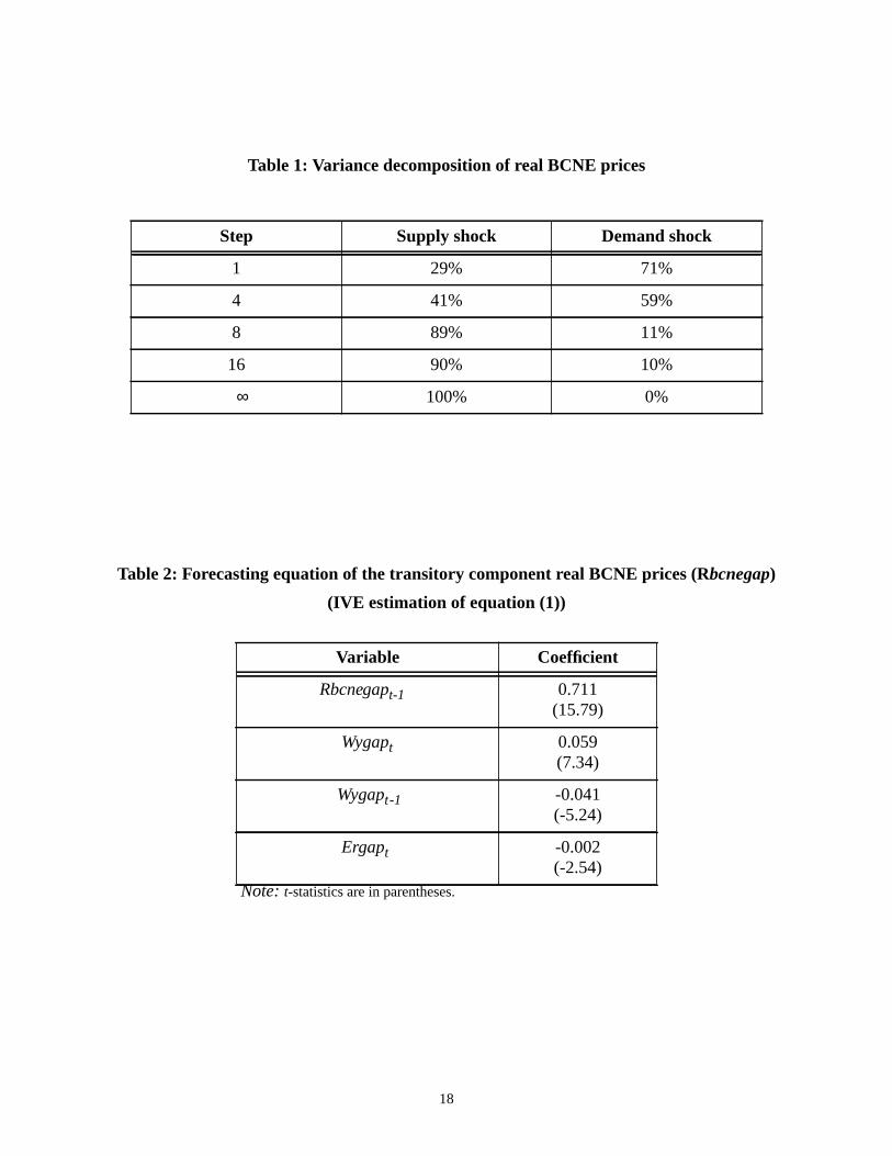
Table 1: Variance decomposition of real BCNE prices
Table 2: Forecasting equation of the transitory component real BCNE prices (Rbcnegap)
(IVE estimation of equation (1))
Note:t-statistics are in parentheses.
Step Supply shock Demand shock
1 29% 71%
4 41% 59%
8 89% 11%
16 90% 10%
∞ 100% 0%
Variable Coefficient
Rbcnegapt-1 0.711(15.79)
Wygapt 0.059(7.34)
Wygapt-1 -0.041(-5.24)
Ergapt -0.002(-2.54)
18
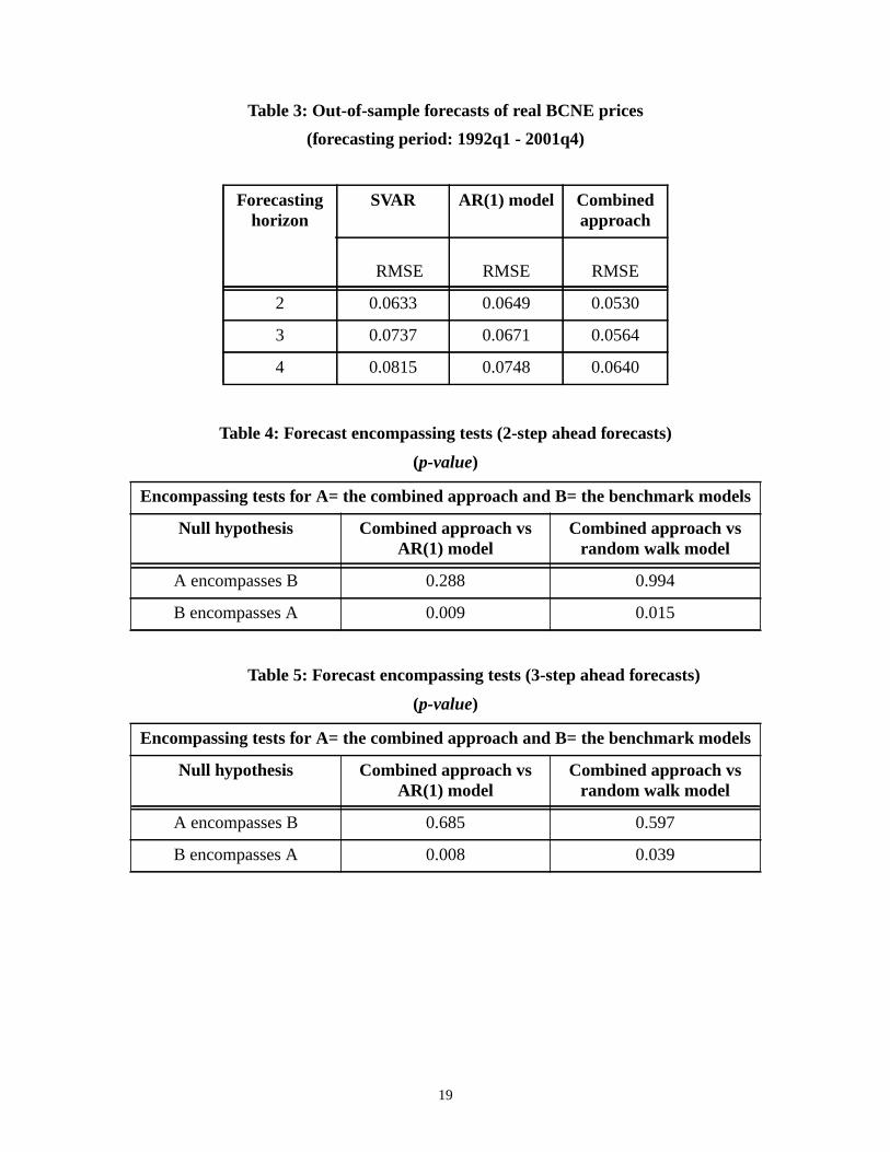
Table 3: Out-of-sample forecasts of real BCNE prices
(forecasting period: 1992q1 - 2001q4)
Table 4: Forecast encompassing tests (2-step ahead forecasts)
(p-value)
Table 5: Forecast encompassing tests (3-step ahead forecasts)
(p-value)
Forecastinghorizon
SVAR AR(1) model Combinedapproach
RMSE RMSE RMSE
2 0.0633 0.0649 0.0530
3 0.0737 0.0671 0.0564
4 0.0815 0.0748 0.0640
Encompassing tests for A= the combined approach and B= the benchmark models
Null hypothesis Combined approach vsAR(1) model
Combined approach vsrandom walk model
A encompasses B 0.288 0.994
B encompasses A 0.009 0.015
Encompassing tests for A= the combined approach and B= the benchmark models
Null hypothesis Combined approach vsAR(1) model
Combined approach vsrandom walk model
A encompasses B 0.685 0.597
B encompasses A 0.008 0.039
19
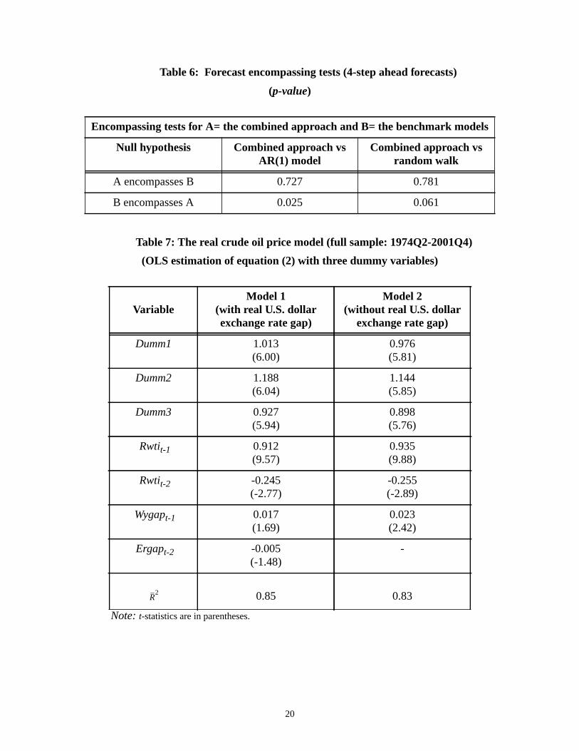
Table 6: Forecast encompassing tests (4-step ahead forecasts)
(p-value)
Table 7: The real crude oil price model (full sample: 1974Q2-2001Q4)
(OLS estimation of equation (2) with three dummy variables)
Note:t-statistics are in parentheses.
Encompassing tests for A= the combined approach and B= the benchmark models
Null hypothesis Combined approach vsAR(1) model
Combined approach vsrandom walk
A encompasses B 0.727 0.781
B encompasses A 0.025 0.061
VariableModel 1
(with real U.S. dollarexchange rate gap)
Model 2(without real U.S. dollar
exchange rate gap)
Dumm1 1.013(6.00)
0.976(5.81)
Dumm2 1.188(6.04)
1.144(5.85)
Dumm3 0.927(5.94)
0.898(5.76)
Rwtit-1 0.912(9.57)
0.935(9.88)
Rwtit-2 -0.245(-2.77)
-0.255(-2.89)
Wygapt-1 0.017(1.69)
0.023(2.42)
Ergapt-2 -0.005(-1.48)
-
0.85 0.83R2
20
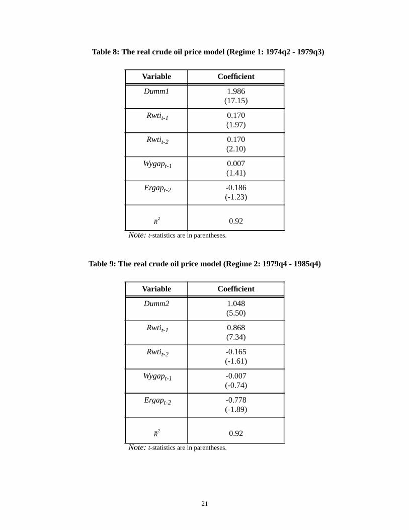
Table 8: The real crude oil price model (Regime 1: 1974q2 - 1979q3)
Note:t-statistics are in parentheses.
Table 9: The real crude oil price model (Regime 2: 1979q4 - 1985q4)
Note:t-statistics are in parentheses.
Variable Coefficient
Dumm1 1.986(17.15)
Rwtit-1 0.170(1.97)
Rwtit-2 0.170(2.10)
Wygapt-1 0.007(1.41)
Ergapt-2 -0.186(-1.23)
0.92
Variable Coefficient
Dumm2 1.048(5.50)
Rwtit-1 0.868(7.34)
Rwtit-2 -0.165(-1.61)
Wygapt-1 -0.007(-0.74)
Ergapt-2 -0.778(-1.89)
0.92
R2
R2
21
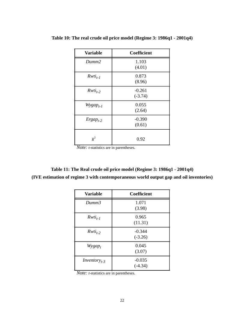
Table 10: The real crude oil price model (Regime 3: 1986q1 - 2001q4)
Note:t-statistics are in parentheses.
Table 11: The Real crude oil price model (Regime 3: 1986q1 - 2001q4)
(IVE estimation of regime 3 with contemporaneous world output gap and oil inventories)
Note:t-statistics are in parentheses.
Variable Coefficient
Dumm2 1.103(4.01)
Rwtit-1 0.873(8.96)
Rwtit-2 -0.261(-3.74)
Wygapt-1 0.055(2.64)
Ergapt-2 -0.390(0.61)
0.92
Variable Coefficient
Dumm3 1.071(3.98)
Rwtit-1 0.965(11.31)
Rwtit-2 -0.344(-3.26)
Wygapt 0.045(3.07)
Inventoryt-3 -0.035(-4.34)
R2
22
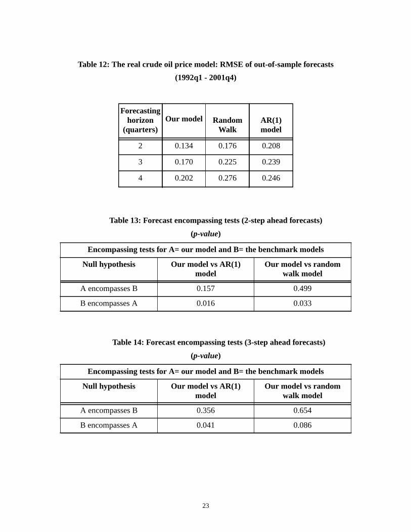
Table 12: The real crude oil price model: RMSE of out-of-sample forecasts
(1992q1 - 2001q4)
Table 13: Forecast encompassing tests (2-step ahead forecasts)
(p-value)
Table 14: Forecast encompassing tests (3-step ahead forecasts)
(p-value)
Forecastinghorizon
(quarters)Our model Random
WalkAR(1)model
2 0.134 0.176 0.208
3 0.170 0.225 0.239
4 0.202 0.276 0.246
Encompassing tests for A= our model and B= the benchmark models
Null hypothesis Our model vs AR(1)model
Our model vs randomwalk model
A encompasses B 0.157 0.499
B encompasses A 0.016 0.033
Encompassing tests for A= our model and B= the benchmark models
Null hypothesis Our model vs AR(1)model
Our model vs randomwalk model
A encompasses B 0.356 0.654
B encompasses A 0.041 0.086
23
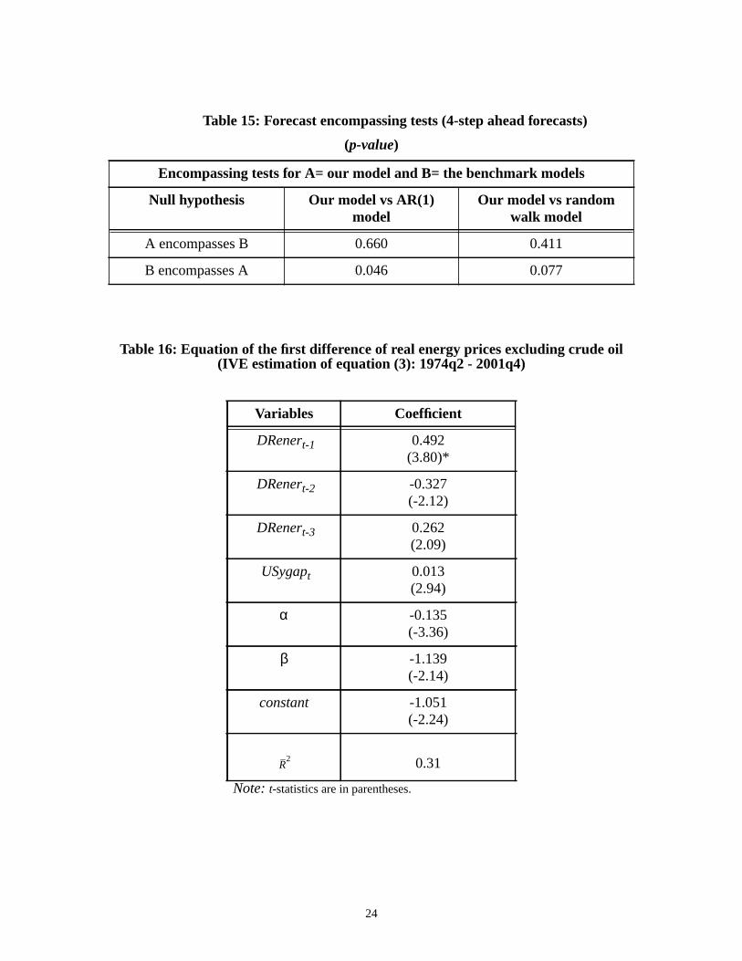
Table 15: Forecast encompassing tests (4-step ahead forecasts)
(p-value)
Table 16: Equation of the first difference of real energy prices excluding crude oil(IVE estimation of equation (3): 1974q2 - 2001q4)
Note:t-statistics are in parentheses.
Encompassing tests for A= our model and B= the benchmark models
Null hypothesis Our model vs AR(1)model
Our model vs randomwalk model
A encompasses B 0.660 0.411
B encompasses A 0.046 0.077
Variables Coefficient
DRenert-1 0.492(3.80)*
DRenert-2 -0.327(-2.12)
DRenert-3 0.262(2.09)
USygapt 0.013(2.94)
α -0.135(-3.36)
β -1.139(-2.14)
constant -1.051(-2.24)
0.31R2
24
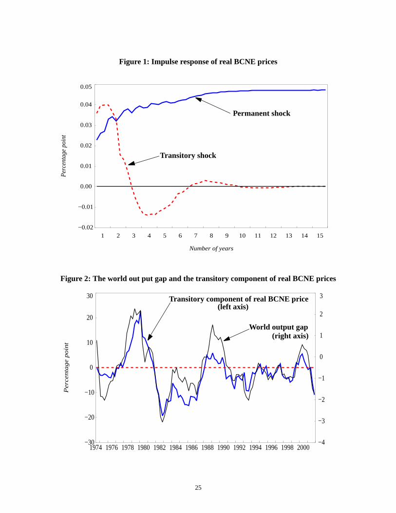
Figure 1: Impulse response of real BCNE prices
Figure 2: The world out put gap and the transitory component of real BCNE prices
−0.02
−0.01
0.00
0.01
0.02
0.03
0.04
0.05
1 2 3 4 5 6 7 8 9 10 11 12 13 14 15
Per
cent
age
poin
t
Number of years
Permanent shock
Transitory shock
1974 1976 1978 1980 1982 1984 1986 1988 1990 1992 1994 1996 1998 2000−30
−20
−10
0
10
20
30
−4
−3
−2
−1
0
1
2
3
Pe
rce
nta
ge
po
int
Transitory component of real BCNE price
World output gap (right axis)
(left axis)
25
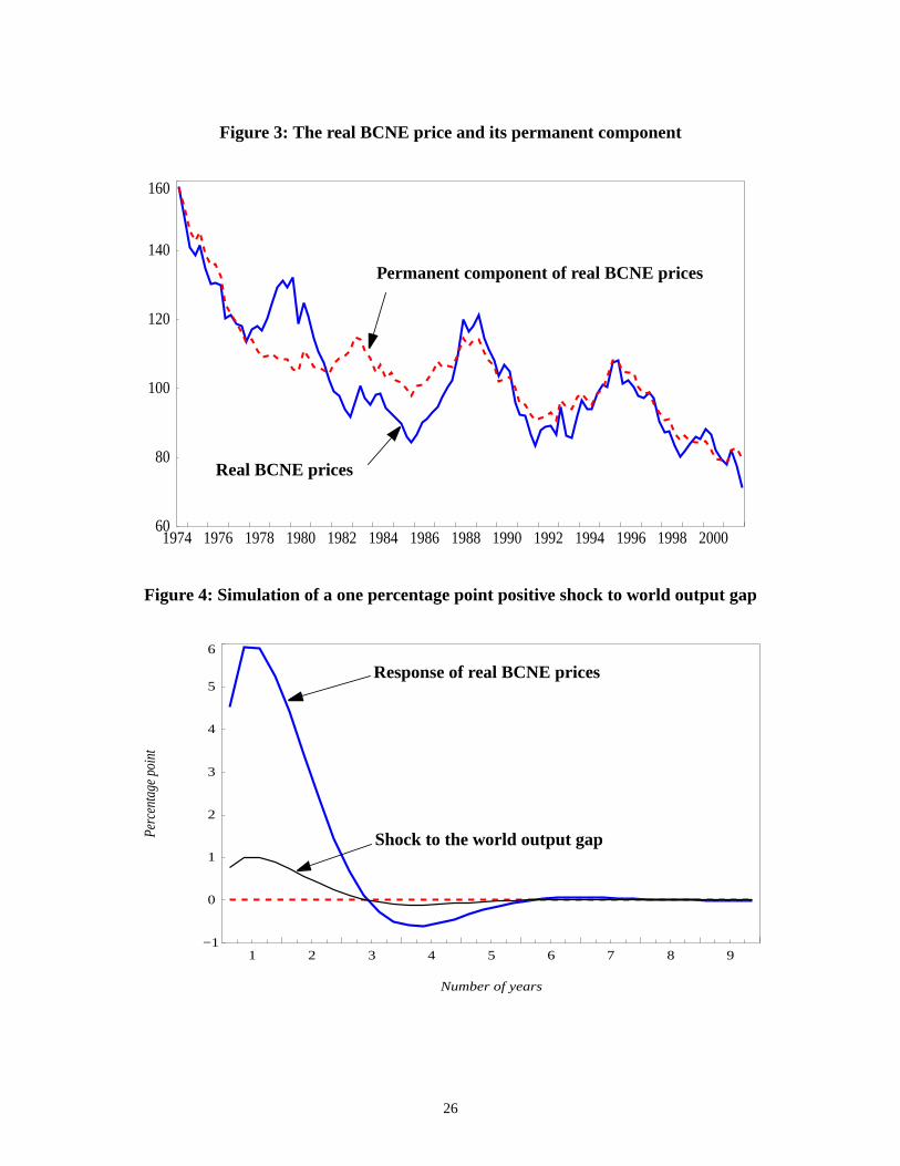
Figure 3: The real BCNE price and its permanent component
Figure 4: Simulation of a one percentage point positive shock to world output gap
1974 1976 1978 1980 1982 1984 1986 1988 1990 1992 1994 1996 1998 200060
80
100
120
140
160
Permanent component of real BCNE prices
Real BCNE prices
−1
0
1
2
3
4
5
6
1 2 3 4 5 6 7 8 9
Per
cent
age
poin
t
Number of years
Shock to the world output gap
Response of real BCNE prices
26
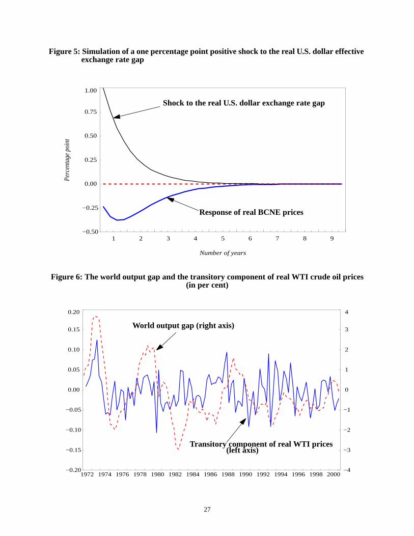
Figure 5: Simulation of a one percentage point positive shock to the real U.S. dollar effective exchange rate gap
Figure 6: The world output gap and the transitory component of real WTI crude oil prices(in per cent)
−0.50
−0.25
0.00
0.25
0.50
0.75
1.00
1 2 3 4 5 6 7 8 9
Per
cent
age
poin
t
Number of years
Shock to the real U.S. dollar exchange rate gap
Response of real BCNE prices
1972 1974 1976 1978 1980 1982 1984 1986 1988 1990 1992 1994 1996 1998 2000−0.20
−0.15
−0.10
−0.05
0.00
0.05
0.10
0.15
0.20
−4
−3
−2
−1
0
1
2
3
4
World output gap (right axis)
Transitory component of real WTI prices(left axis)
27

Figure 7: Simulation of a one per cent positive shock to the world output gap
(Regime 3)
−0.5
0.0
0.5
1.0
1.5
−5
0
5
10
15
1 2 3 4 5 6 7 8 9 10
Per
cent
age
poin
ts
Number of years
Response of real WTI crude oil prices
Shock to the world output gap (left axis)
(right axis)
28
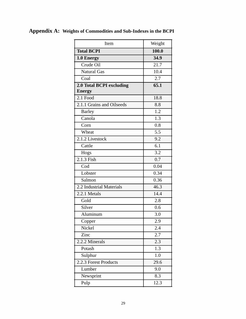
Appendix A: Weights of Commodities and Sub-Indexes in the BCPI
Item Weight
Total BCPI 100.01.0 Energy 34.9
Crude Oil 21.7
Natural Gas 10.4
Coal 2.7
2.0 Total BCPI excludingEnergy
65.1
2.1 Food 18.8
2.1.1 Grains and Oilseeds 8.8
Barley 1.2
Canola 1.3
Corn 0.8
Wheat 5.5
2.1.2 Livestock 9.2
Cattle 6.1
Hogs 3.2
2.1.3 Fish 0.7
Cod 0.04
Lobster 0.34
Salmon 0.36
2.2 Industrial Materials 46.3
2.2.1 Metals 14.4
Gold 2.8
Silver 0.6
Aluminum 3.0
Copper 2.9
Nickel 2.4
Zinc 2.7
2.2.2 Minerals 2.3
Potash 1.3
Sulphur 1.0
2.2.3 Forest Products 29.6
Lumber 9.0
Newsprint 8.3
Pulp 12.3
29
ws:
d the
at we
and a
hock
lifi-
(i.e.
4)
Appendix B: The Blanchard-Quah (1989) decomposition and the link betweenthe structural form and the reduced form of the model
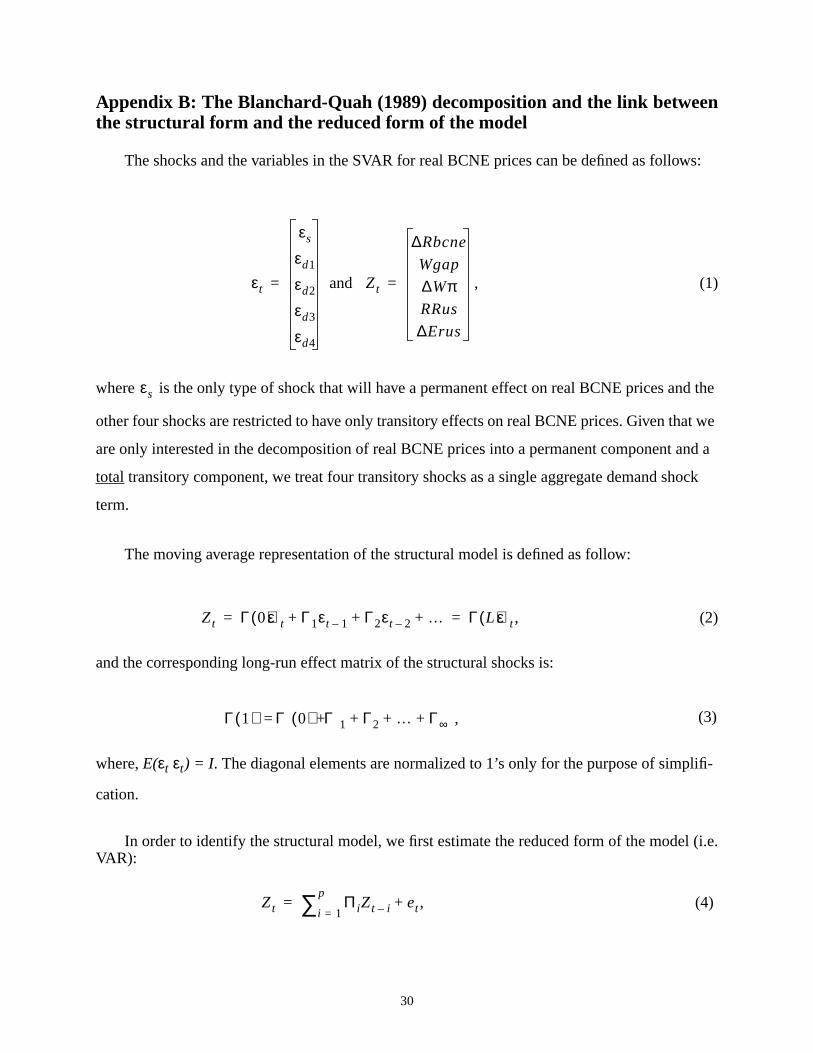
The shocks and the variables in the SVAR for real BCNE prices can be defined as follo
and , (1)
where is the only type of shock that will have a permanent effect on real BCNE prices an
other four shocks are restricted to have only transitory effects on real BCNE prices. Given th
are only interested in the decomposition of real BCNE prices into a permanent component
total transitory component, we treat four transitory shocks as a single aggregate demand s
term.
The moving average representation of the structural model is defined as follow:
, (2)
and the corresponding long-run effect matrix of the structural shocks is:
,
where,E(εt εt) = I . The diagonal elements are normalized to 1’s only for the purpose of simp
cation.
In order to identify the structural model, we first estimate the reduced form of the modelVAR):
, (
εt
εs
εd1
εd2
εd3
εd4
= Zt
∆Rbcne
Wgap
∆WπRRus
∆Erus
=
εs
Zt Γ 0( )εt Γ1εt 1– Γ2εt 2– …+ + + Γ L( )εt= =
Γ 1( ) Γ 0( ) Γ1 Γ2 … Γ∞+ + + +=
Zt ΠiZt i–i 1=
p∑ et+=
(3)
30
re
uation
in the
tions
ctural
d
ents
n the
d
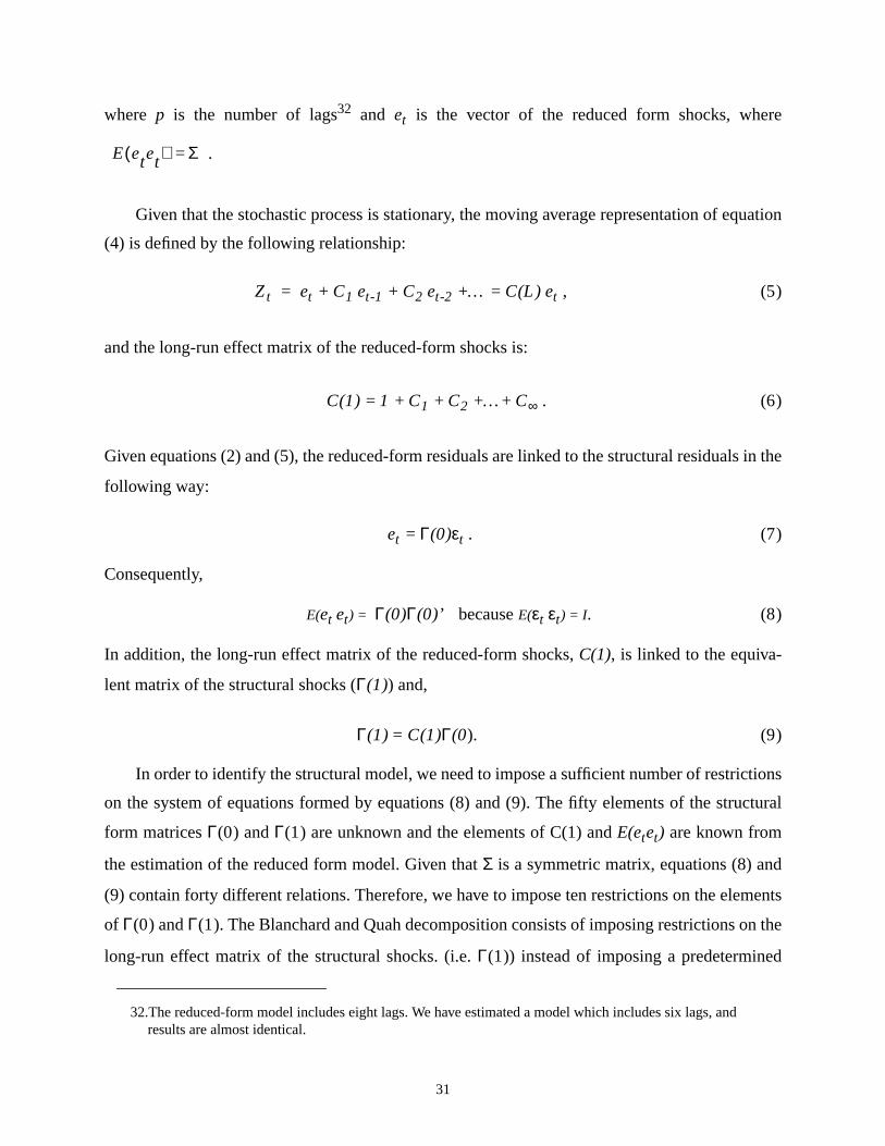
where p is the number of lags32 and et is the vector of the reduced form shocks, whe
.
Given that the stochastic process is stationary, the moving average representation of eq
(4) is defined by the following relationship:
Zt = et + C1 et-1 + C2 et-2 +… = C(L) et , (5)
and the long-run effect matrix of the reduced-form shocks is:
C(1) = 1 + C1 + C2 +…+ C∞ . (6)
Given equations (2) and (5), the reduced-form residuals are linked to the structural residuals
following way:
et = Γ(0)εt . (7)
Consequently,
E(et et) = Γ(0)Γ(0)’ becauseE(εt εt) = I . (8)
In addition, the long-run effect matrix of the reduced-form shocks,C(1), is linked to the equiva-
lent matrix of the structural shocks (Γ(1)) and,
Γ(1) = C(1)Γ(0). (9)
In order to identify the structural model, we need to impose a sufficient number of restric
on the system of equations formed by equations (8) and (9). The fifty elements of the stru
form matricesΓ(0) andΓ(1) are unknown and the elements of C(1) andE(etet) are known from
the estimation of the reduced form model. Given thatΣ is a symmetric matrix, equations (8) an
(9) contain forty different relations. Therefore, we have to impose ten restrictions on the elem
of Γ(0) andΓ(1). The Blanchard and Quah decomposition consists of imposing restrictions o
long-run effect matrix of the structural shocks. (i.e.Γ(1)) instead of imposing a predetermine
32.The reduced-form model includes eight lags. We have estimated a model which includes six lags, andresults are almost identical.
E etet( ) Σ=
31
t
) and
s the
ation
model,
n real
com-
levant
r
sump-
long-
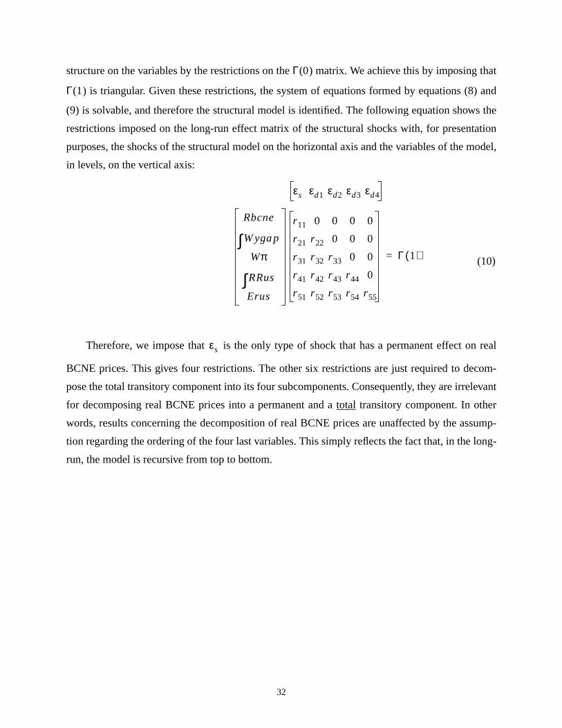
structure on the variables by the restrictions on theΓ(0) matrix. We achieve this by imposing tha
Γ(1) is triangular. Given these restrictions, the system of equations formed by equations (8
(9) is solvable, and therefore the structural model is identified. The following equation show
restrictions imposed on the long-run effect matrix of the structural shocks with, for present
purposes, the shocks of the structural model on the horizontal axis and the variables of the
in levels, on the vertical axis:
Therefore, we impose that is the only type of shock that has a permanent effect o
BCNE prices. This gives four restrictions. The other six restrictions are just required to de
pose the total transitory component into its four subcomponents. Consequently, they are irre
for decomposing real BCNE prices into a permanent and atotal transitory component. In othe
words, results concerning the decomposition of real BCNE prices are unaffected by the as
tion regarding the ordering of the four last variables. This simply reflects the fact that, in the
run, the model is recursive from top to bottom.
Rbcne
W∫ ygap
Wπ
R∫ Rus
Erus
r11 0 0 0 0
r21 r22 0 0 0
r31 r32 r33 0 0
r41 r42 r43 r44 0
r51 r52 r53 r54 r55
Γ 1( )=
εs εd1 εd2 εd3 εd4
εs
(10)
32
l
-
is
hen
least
coeffi-
e
ative
duals
mini-
gth of
ks are
st
Appendix C: Technical details on Bai and Perron (1995) methodology
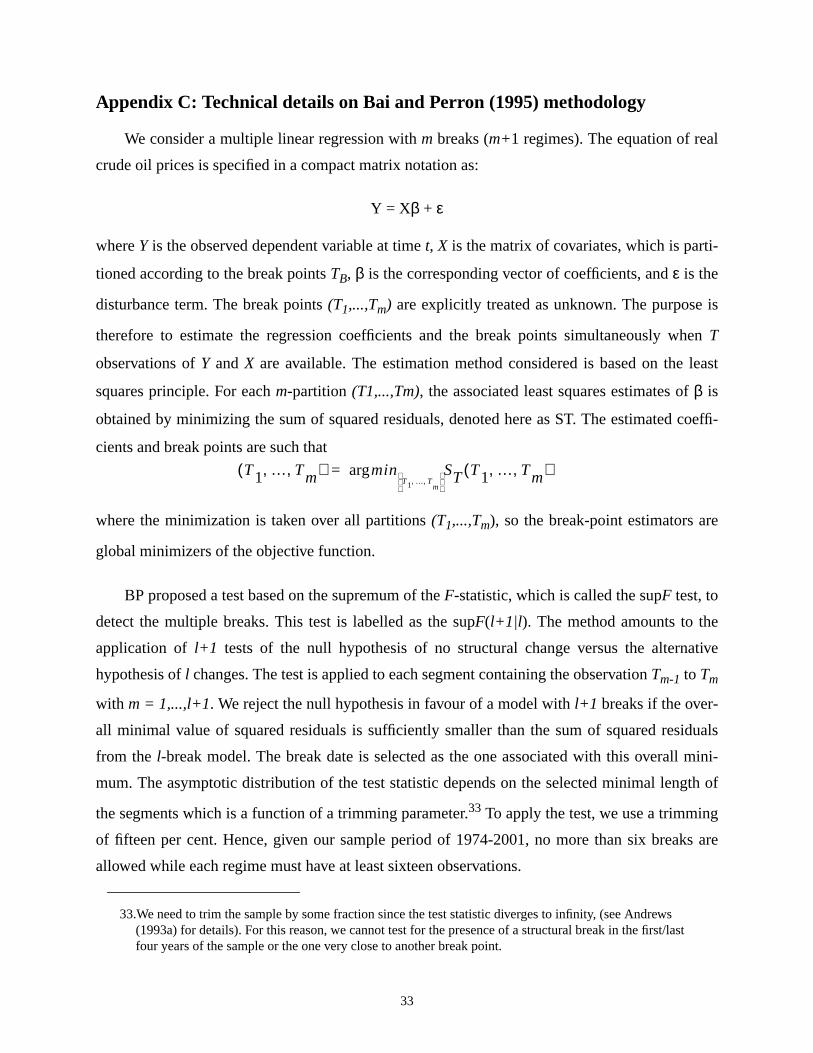
We consider a multiple linear regression withm breaks (m+1 regimes). The equation of rea
crude oil prices is specified in a compact matrix notation as:
Y = Xβ + ε
whereY is the observed dependent variable at timet, X is the matrix of covariates, which is parti
tioned according to the break pointsTB, β is the corresponding vector of coefficients, andε is the
disturbance term. The break points(T1,...,Tm) are explicitly treated as unknown. The purpose
therefore to estimate the regression coefficients and the break points simultaneously wT
observations ofY andX are available. The estimation method considered is based on the
squares principle. For eachm-partition (T1,...,Tm), the associated least squares estimates ofβ is
obtained by minimizing the sum of squared residuals, denoted here as ST. The estimated
cients and break points are such that
where the minimization is taken over all partitions(T1,...,Tm), so the break-point estimators ar
global minimizers of the objective function.
BP proposed a test based on the supremum of theF-statistic, which is called the supF test, to
detect the multiple breaks. This test is labelled as the supF(l+1|l ). The method amounts to the
application of l+1 tests of the null hypothesis of no structural change versus the altern
hypothesis ofl changes. The test is applied to each segment containing the observationTm-1 to Tm
with m = 1,...,l+1. We reject the null hypothesis in favour of a model withl+1 breaks if the over-
all minimal value of squared residuals is sufficiently smaller than the sum of squared resi
from the l-break model. The break date is selected as the one associated with this overall
mum. The asymptotic distribution of the test statistic depends on the selected minimal len
the segments which is a function of a trimming parameter.33 To apply the test, we use a trimming
of fifteen per cent. Hence, given our sample period of 1974-2001, no more than six brea
allowed while each regime must have at least sixteen observations.
33.We need to trim the sample by some fraction since the test statistic diverges to infinity, (see Andrews(1993a) for details). For this reason, we cannot test for the presence of a structural break in the first/lafour years of the sample or the one very close to another break point.
T1 … Tm, ,( ) minT1 … T, ,
m ST T1 … Tm, ,( )arg=
33