Forecasting commodity futures using

Principal Component Analysis and Copula

Martin Jacobsson

May 20, 2015

Abstract

The ever ongoing battle to beat the market is in this thesis fought withthe help of mathematics with a way to reduce the information to its core.It is called PCA, Principal Component Analysis. This is used to build amodel of future commodity prices. To assist PCA, Copula is used - a sortof mathematical glue which can bring multiple distributions together andrepresented as one.

The data used is 5 years of prices for Brent Oil, WTI Oil, Gold, Copperand Aluminium. The model parameters are fitted to 2.5 years of data andthen tested on the remaining 2.5 years.

MLE, Maximum Likelihood Estimation, was used for parameter estima-tion and distributions that were found fitting were logistic and Student’s Tdistribution

Cramer-von Mises tests were used to determine that T Copula was themost suitable Copula.

The main results are that the mathematical estimations fit well andprofit can be generated, but with a low Sharpe Ratio.

Keywords: PCA, Copula, Mean-reversion, Momentum, Elliptical copu-las, Maximum Likelihood, Cramer-von Mises, Sharpe Ratio.

Acknowledgements

I would like to thank my supervisor Associate Professor Nader Tajvidi atLund University and my supervisor Thomas Lyse Hansen at Nordea for alltheir help and guidance. I also want to extend my gratitude to my familyand friends for all their support. Finally, my special thanks goes to VikingJacobsson for all the invaluable help.

Contents

1 Introduction 41.1 Purpose . . . . . . . . . . . . . . . . . . . . . . . . . . . . . . 41.2 The commodity market . . . . . . . . . . . . . . . . . . . . . 41.3 Futures contract . . . . . . . . . . . . . . . . . . . . . . . . . 51.4 Overview . . . . . . . . . . . . . . . . . . . . . . . . . . . . . 51.5 Hypothesis . . . . . . . . . . . . . . . . . . . . . . . . . . . . 5

2 Theory 62.1 Log returns . . . . . . . . . . . . . . . . . . . . . . . . . . . . 62.2 Principal Components Analysis (PCA) . . . . . . . . . . . . . 72.3 Mean-reverting Theory . . . . . . . . . . . . . . . . . . . . . . 82.4 Momentum . . . . . . . . . . . . . . . . . . . . . . . . . . . . 92.5 Copula . . . . . . . . . . . . . . . . . . . . . . . . . . . . . . . 102.6 Elliptical Copulas . . . . . . . . . . . . . . . . . . . . . . . . . 12

2.6.1 Gaussian Copula . . . . . . . . . . . . . . . . . . . . . 122.6.2 Student’s T Copula . . . . . . . . . . . . . . . . . . . 12

2.7 Distributions . . . . . . . . . . . . . . . . . . . . . . . . . . . 132.7.1 Generalised Logistic Distribution . . . . . . . . . . . . 132.7.2 Student’s T Distribution . . . . . . . . . . . . . . . . . 13

2.8 Dependence Theory . . . . . . . . . . . . . . . . . . . . . . . 142.8.1 Concordance . . . . . . . . . . . . . . . . . . . . . . . 152.8.2 Kendall’s Tau . . . . . . . . . . . . . . . . . . . . . . . 15

2.9 Parameter Estimation . . . . . . . . . . . . . . . . . . . . . . 152.9.1 Maximum Likelihood Estimation . . . . . . . . . . . . 16

2.10 Goodness of Fit . . . . . . . . . . . . . . . . . . . . . . . . . . 162.10.1 Quantile-Quantile Plot . . . . . . . . . . . . . . . . . . 162.10.2 Cramer-von Mises Method . . . . . . . . . . . . . . . . 16

2.11 Portfolio Return . . . . . . . . . . . . . . . . . . . . . . . . . 172.12 Sharpe Ratio . . . . . . . . . . . . . . . . . . . . . . . . . . . 17

2

3 Implementation and Results 193.1 The Data Set . . . . . . . . . . . . . . . . . . . . . . . . . . . 193.2 Implementation . . . . . . . . . . . . . . . . . . . . . . . . . . 223.3 Part One - PCA . . . . . . . . . . . . . . . . . . . . . . . . . 223.4 Part Two - Copula . . . . . . . . . . . . . . . . . . . . . . . . 243.5 Part Three - PCA and Copula Combined . . . . . . . . . . . 29

4 Discussion 314.1 Summary . . . . . . . . . . . . . . . . . . . . . . . . . . . . . 314.2 Tradeable Results . . . . . . . . . . . . . . . . . . . . . . . . . 324.3 The Future . . . . . . . . . . . . . . . . . . . . . . . . . . . . 334.4 Conclusion . . . . . . . . . . . . . . . . . . . . . . . . . . . . 33

5 References 345.1 Reference List . . . . . . . . . . . . . . . . . . . . . . . . . . . 34

3

Chapter 1

Introduction

Many financial traders around the world struggle with the same question:how can I beat the market? If one could come up with one easy way to dothis, their financial problems would forever be gone. An approach to modelthe reality is in this thesis done with the help of PCA and Copula - twomathematical tools.

1.1 Purpose

The purpose of this Master’s Thesis is to see if the prediction model pre-sented will be able to generate a positive risk-adjusted absolute return ornot. To measure this, Sharpe Ratio is used. Since Sharpe Ratio includesthe risk-free rate rf , we set rf = 0 due to our only interest in absoluterisk-adjusted return.

1.2 The commodity market

The commodity market is one of the oldest (if not the oldest) and mostfundamental markets in the world. One could say that the commodity mar-ket was the start of our civilized society [Banerjee, 2013]. It was there thatpeople first learned to trade with their own specialized good in order toprocure another good which they needed. The first commodity trading ac-tivities stretch back to the ancient Sumerian civilization between 4,500 BCand 4,000 BC. They then used clay tokens to represent the number of goodsto be delivered, for example the number of goats. These clay tokens werethen sealed in a vessel to represent the promise they had made to deliver xnumber of goats.

4

Nowadays, the commodity market is a vast system of different marketsall over the world where a future delivery of gold or corn just are some clickson your computer away. Naturally, the greatest price factor is supply anddemand, but this thesis will try to investigate if one can use mathematicaltools to forecast the price movements.

1.3 Futures contract

To procure the wanted commodity, the most used way is to use so calledfutures. A futures contract is a standardized contract between two parties,which settles for a specified asset with a certain price today but with afuture specified delivery and payment date [Hull, 2009]. Due to a defaultrisk, both parties are required to put up a margin - the initial amount ofcash. During a change in the futures price, these margins are transferredbetween the parties, generally once a day. This means that all profits andlosses are settled continuously so at the delivery date, the exchanged amountis the spot price(the price for getting something right away) [Hull, 2009] ofthe underlying asset. Consequently, to take a position in a futures contractis free, excluded transaction costs such as brokerage fees.

1.4 Overview

In the forecasting model Principal Component Analysis and Copula will beused to generate buy and sell signals. These signals will then be used indifferent types of trading strategies where profit can be generated as theprice goes up as well as when the price goes down. A total Sharpe ratio willbe calculated of these strategies to evaluate the performance.

1.5 Hypothesis

The hypothesis is that the presented forecasting model will be able to gen-erate a positive risk-adjusted return.

5

Chapter 2

Theory

In this chapter all the necessary theoretical background for the predictionmodel is presented. The chapter starts out with theory regarding log re-turns and PCA. Thereafter the main trading strategies are introduced -mean reversion and momentum strategies. Then more mathematical the-ory is presented; Copula, Elliptical Copulas and distributions. Moreover,Dependence Theory, Parameter Estimation and Goodness of Fit test arepresented. Lastly, we will introduce the concept of Sharpe Ratio which is arisk adjusted performance measure.

2.1 Log returns

In this thesis log returns are used which have several advantages. Below arethe main two reasons:

• There is a normalization of the variables, which means that all returnsare in a comparable metric.

• Log returns are time additive, which means that to get the n-periodreturn - we can simply add all the single period returns up to n.

To calculate the log returns the following equation is used.

ri,t = lnPi,tPi,t−1

, i = 1, ..., n (2.1)

where Pi,t is the price of the futures contract - i indicates which of thecommodities used at a given time t.

6

2.2 Principal Components Analysis (PCA)

To introduce Principal Components Analysis, we take the following excerptfrom [Jolliffe, 2002]:

”The central idea of principal component analysis (PCA) is to reducethe dimensionality of a data set consisting of a large number of interrelatedvariables, while retaining as much as possible of the variation present in thedata set. This is achieved by transforming to a new set of variables, theprincipal components (PC’s), which are uncorrelated and which are orderedso that the first few retain most of the variation present in all of the originalvariables.”

With this concise explanation as a start, we are now ready for the defi-nition of PCA.

Definition 1. Suppose that x is a vector of p random variables. Thefirst step is to look for a linear function α′1x of the elements of x having amaximum variance, where α1 is a vector of p constants α11, ..., α12, α1p, and”′” denotes transpose, so that

α′1x = α11x1 + α12x2 + ...+ α1pxp =

p∑j=1

α1jxj (2.2)

Then, we look for a linear function α′2x, uncorrelated with α′1x having max-imum variance, and so on, so that the k-th stage a linear function α′kxis found that has maximum variance subject to being uncorrelated withα′1x, α

′2x, ..., α

′k−1x. The k-th derived variable, α′kx is the k-th PC and p is

the number of commodities.

So, depending on what we choose k to be - we get k number of PC’s.In this case we set the x in the above definition as y - the de-meaned logreturns.

y = x− xmean (2.3)

where xmean is the mean of x.

When we then project these vectors back on to our data, we get theD-matrix.

D = AT · y (2.4)

7

where A = (a1, ..., ak)

We will later use this matrix D, which is the matrix of dimensionally reducedreturns, obtained after projecting y in the principal component space.

2.3 Mean-reverting Theory

In this trading model, two main trading strategies are used. The first iscalled mean-reversion strategy [Investopedia, 2015] and is simply the theorythat prices should move back towards their moving average(their mean cal-culated a constant x days back). As [Infantino et al., 2010] discusses thisis perhaps the most simple of all trading strategies but it does not take thebehavioural aspect of trading into account. The mean reversion theory isused in this thesis as a foundation of the PCA. Our PCA gives us a firstmodel which tells us how the returns without noise should have been the lastperiod. We then act accordingly - if the model tells us that the prices aretoo high, we sell and vice versa. Studies that mean reversion theory worksand actually generates alpha in commodity prices are discussed in [Lutz,2010] which is taken into account in this prediction model.Main input parameters into our model are; the T number of days we arelooking back at, the H future days of returns, the k number of principalcomponents.

The following formula is the foundation of the mean reverting section.

rt+1 + ...+ rt+H = β1

H∑i=0

Dt−i,1 + ...+ βk

H∑i=0

Dt−i,k (2.5)

where rt is the log return at time t, β is the factor that explains the ratiobetween the log returns and the matrix D. That is, the β values want to ex-plain the connection between past periods PC’s and coming periods returns.

We define a matrix B which includes all the β’s with dimensions k×number of commodities.

We also define the matrix Dt - the sum of the returns from the D-matrix:

Dt =

H−1∑i=0

Dt−i, t = (1, 2, ..., T ) (2.6)

8

Finally, we get our prediction of the future log return S as,

St = Dt ·B (2.7)

So if this S is higher than the actual log return, we sell and vice versa. Weget a long list of buy or sell signals, and the momentum strategy statedbelow can overwrite those signals.

2.4 Momentum

In this model, the behavioural aspect of trading is represented by a momen-tum strategy, which is the belief that if a price is in an upward trend, itwill continue going up. Likewise if the price is falling, momentum strategiesstates that it will continue falling. In short, you could say that it is a ”ride-the-wave” type of trading mindset - contradictory to the mean-reversiontheory. In [Jegadeesh et al., 1999] it is shown that financial instrumentswith strong past performance continue to outperform those with poor pastperformance. This momentum theory is implemented into our predictionmodel.

To introduce the momentum strategy into our model, we use [Infantinoet al., 2010] ”the Cross Sectional Volatility of the Principal Components”,which is the standard deviation σD(t) of the returns, projected onto theprincipal components. Briefly you could say that we want to look at if therate of change in the discrete time (Euclidean distance EH - defined below)grows. More specifically:

σD(t) =

√√√√ k∑j=1

(dtj − dt)2

k − 1, t = (1, 2, ..., T ) (2.8)

where k is the number of principal components, dtj is the reduced-dimensionality

return j at time t and dt is the cross sectional mean:

dt =1

k

k∑j=1

dtj (2.9)

We want to look at the changes in time, the derivative, to see if thereare great changes in the standard deviation. To decide if there are ”great

9

changes” we define a measure ψ for the change of the standard deviationcompared to time.

ψ =dσDdt

(2.10)

To get a distance measure we define EH :

EH(t) =

√√√√ H∑i

[ψ(t− i)]2 (2.11)

Finally, to decide if we are in a ”momentum” or not and to decide if weshould override the mean-reverting signal, we check:

EH(t)− EH(t− 1) (2.12)

So if this is less than or equal to zero, we continue with the mean-reverting signal. Else, we switch so that we apply the momentum strategyand continue ”riding-the-wave”.

2.5 Copula

To be able to study all our fitted distributions of our commodity prices,one can use copula as a glue for these distributions. This is more formallydescribed below, from [Nelsen, 2006] first for a bivariate copula and then forthe n-dimensional case.

Definition 2. A two-dimensional subcopula is a function C ′ with fol-lowing properties:

• DomC ′ = S1 × S2, where S1 and S2 are subsets of I containing 0 and1.

• C ′ is grounded and 2-increasing.

• For every u in S1 and and every v in S2,

C ′(u, 1) = u and C ′(1, v) = v. (2.13)

Definition 3. A two-dimensional copula is a 2-subcopula C whosedomain is I2.

Equivalently, a copula is a function C from I2 to I with the followingproperties:

10

• For every u, v in I,

C(u, 0) = 0 = C(0, u),

C(u, 1) = u,C(1, v) = v.

• For every u1, u2, v1 and v2 in I such that u1 ≤ u2, v1 ≤ v2

C(u2, v2)− C(u2, v1)− C(u1, v2) + C(u1, v1) ≥ 0. (2.14)

This is called the rectangle inequality of copula.

From [Nelsen, 2006] we find the theorems regarding Frechet-Hoeffdingbounds.

Theorem 1 (Frechet-Hoeffding bounds in 2-dimensions). Let C ′ be asubcopula. Then for every (u, v) in DomC ′

max(u+ v − 1, 0) ≤ C ′(u, v) ≤ min(u, v) (2.15)

The n-dimensional case follows from [Nelsen, 2006]Theorem 2 (Frechet-Hoeffding bounds in n-dimensions). Let C be a

copula, then the following inequality is satisfied,

max(u1 + u2 + ...+ un − d+ 1, 0) ≤ C(u) ≤ min(u1, u2, ..., un). (2.16)

where u ∈ [0, 1]n

Theorem 3 (Sklar’s theorem).Let H be an n-dimensional distributionfunction with margins F1, F2, ..., Fn. Then there exists a n-copula C suchthat for all x in Rn,

H(x1, x2, ..., xn) = C(F1(x1), F2(x2), ..., Fn(xn)). (2.17)

If F1, F2, ..., Fn are all continuous, then C is unique; otherwise C isuniquely determined on Ran F1× Ran F2× ... × Ran Fn. Conversely, if Cis a n-copula and F1, F2, ..., Fn are distribution functions, then the functionH defined by (2.16) is a n-dimensional distribution function with marginsF1, F2, ..., Fn.

11

2.6 Elliptical Copulas

One can describe the elliptical copulas (named so for their elliptical contourshape) as the most basic of copulas. One advantage that is used in thisthesis is that they can handle both positive and negative dependence.

To describe the dependence structure for elliptical copulas, the notationof Σ is used to represent the correlation matrix. Elliptical copulas have thefollowing relationship between its dependence parameter and Kendall’s Tau.

τK =2

πarcsinρ (2.18)

where ρ is the corresponding ”off-diagonal” parameter of dependence in Σ.

2.6.1 Gaussian Copula

As defined in [Bouye, 2000] the definition for multivariate gaussian copula(MVN) is the following.

Definition 4.Let ρ be a symmetric, positive definite matrix with diag ρ = 1 and Φρ

the standardized multivariate normal distribution with correlation matrixρ. The multivariate gaussian copula is the defined as follows:

C(u1, ..., un, ..., uN ; ρ) = Φρ(Φ−1(u1), ...,Φ−1(un), ...,Φ−1(uN )) (2.19)

The density of the gaussian copula is then defined as follows.

Definition 5.

c(u1, ..., un, ..., uN ; ρ) =1

| ρ |12

exp(− 12ζT (ρ−1−I)ζ) (2.20)

where ζn = Φ−1(un)

2.6.2 Student’s T Copula

Continuing with the writings from [Bouye, 2000], the multivariate Student’sT Copula (MVT) is defined as follows.

Definition 6.C(u1, ..., un, ..., uN ; ρ, ν) = Tρ,ν(tν

−1(u1), ..., tν−1(un), ..., tν

−1(uN )) (2.21)

12

with tν−1 as the inverse of the univariate Student’s T distribution.

Corresponding density is

Definition 7.

c(u1, ..., un, ..., uN ; ρ, ν) = | ρ |−12

Γ(ν+N2 [Γν

2 ]N )(1 + 1ν ζ

Tρ−1ζ)−ν+N

2

[Γ(ν+12 )]NΓ(ν2 )

N∏n=1

(1 +ζn

2

ν)−

ν+12

(2.22)

2.7 Distributions

Below are the distributions that were fitted to the log returns of the com-modities. Both logistic distribution and Student’s T distribution are knownto have fatter tails than the normal distribution, which suited the log re-turns.

2.7.1 Generalised Logistic Distribution

In [Shao, 2002] the generalised logistic distribution is described with thefollowing density function.

fGL1(x; θ, σ, α) =α

σ∗ e−(x−θ)/σ

(1 + e−(x−θ)/σ)α+1, (2.23)

where θ is the location parameter, σ > 0 is the scale and α > 0 is the shapeparameter.

2.7.2 Student’s T Distribution

As described in [Jackman, 2009] the Student’s T distribution is defined asfollows.

Definition 8.If x follows a (standardized) Student’s T density with ν > 0 degrees offreedom, conventionally written x ∼ tν , then

p(x) =Γ((ν + 1)/2)

Γ(ν/2)√νπ

(1 +x2

ν)−(ν+1)/2 (2.24)

13

and has mean 0 and variance ν/(ν − 2).In unstandardised form, the Student’s T density is

p(x) =Γ((ν + 1)/2)

Γ(ν/2)σ√νπ

(1 +1

ν(x− µσ

)2)−(ν+1)/2 (2.25)

and is conventionally written x ∼ tν(µ, σ2), where µ is a location param-eter, σ > 0 is a scale parameter and ν > 0 is a degree of freedom parameter.

• The standardized version of the T density is and unstandardised Tdensity with µ = 0 and σ = 1.

• Provided ν > 1, E(x) = µ and V (x) = νν−2σ

2.

• As ν →∞, p(x) tends to the normal density.

2.8 Dependence Theory

There are different types of dependence measures but the most common iscalled linear correlation, or more formally - Pearson’s correlation coefficient.This is calculated through,

ρX,Y =cov[X,Y ]√

V ar[X]V ar[Y ](2.26)

But this dependence measure has three main disadvantages.

• It requires that mean and variance exists, else it is useless.

• It can only measure linear dependence between X and Y , so a modi-fication in X must have a likewise constant proportional modificationin Y .

• It is not invariant to non-linear transformations.

So this is called correlation coefficient but when we are talking aboutscale-invariant measures of dependence we call them measures of associa-tion. One of the main measure of association - Kendall’s Tau, is presentedbelow (Spearman’s Rho is not used in this thesis, hence the lack of defini-tion).

14

2.8.1 Concordance

To define Kendall’s Tau, we need to explain what concordance is, which ispresented in [Nelsen, 2006],

Briefly, you could say that a pair of random variables are concordant if largevalues of one tend to be associated with large values of the other. Likewise,small values of one tend to be associated with small values of the other.This is presented more accurately below.

Let (xi, yi) and (xj , yj) denote two observations from a vector (X,Y ) ofcontinuous random variables. We say that (xi, yi) and (xj , yj) are concordantif xi < xj and yi < yj , or if xi > xj and yi > yj . Similarly, we say that(xi, yi) and (xj , yj) are discordant if xi < xj and yi > yj , or if xi > xj andyi < yj .

2.8.2 Kendall’s Tau

We are now ready to define the measure of association Kendall’s Tau interms of concordance and discordance.

Definition 9.Let [(x1, y1), (x2, y2), ..., (xj , yj)] denote a random sample of n observationsfrom a vector (X,Y) of continuous random variables. There are

(n2

)distinct

pairs (xi, yi) and (xj , yj) of observations in the sample, and each pair iseither concordant or discordant. Let c denote the number of concordantpairs and d denote the number of discordant pairs. Then Kendall’s Tau isdefined as,

τK =c− dc+ d

= (c− d)/

(n

2

)(2.27)

2.9 Parameter Estimation

To estimate the parameters of both the margins of commodity prices andthe copulas Maximum Likelihood Estimation (MLE) is used.

15

2.9.1 Maximum Likelihood Estimation

In [Myung, 2003] maximum likelihood estimation is the process of finding avalue θ which is the estimation that makes the underlying data as plausibleas possible. Generally, let x1, ..., xn be i.i.d observations of a random vari-able X with density function f(x; θ), where θ is an unknown parameter inthe space ΩΘ. Then, the corresponding likelihood function Lx(θ) is definedas follows,

Definition 10.

Lx(θ) =

n∏k=1

f(xk; θ). (2.28)

and the MLE is the parameter θmle which maximizes Lx(θ). Hence,

θmle = argmaxθ Lx(θ). (2.29)

2.10 Goodness of Fit

To determine if you have found a fitting model or not, several tests can bedone. In order to determine if we had fitted our probability distributionswell, Quantile-Quantile plots are used. And to test whether a copula C canbe represented in a multivariate distribution, the Cramer-von Mises Methodis used. More on this below.

2.10.1 Quantile-Quantile Plot

The Quantile-Quantile Plot (QQ-plot called henceforth) is a graphical testmethod to see whether our data fits to a distribution or not. The empiricalquantiles are plotted against the quantiles of the fitted theoretical distribu-tion, the points will lie on the line of a 45 degree slope.

2.10.2 Cramer-von Mises Method

To test the goodnes of fit for a copula, one can use the Cramer-von Misesmethod. This method [Genest et al., 2009] is originally based on the ”em-pirical copula” as

16

Cn(u) =1

n

n∑i=1

l(Ui1 ≤ u1, ..., Uid ≤ ud), (2.30)

where u = (u1, ..., ud) in [0, 1]d.

Then, the goodness of fit test process is based on the empirical process

Cn(u) =√n(Cn − Cθ,n) (2.31)

where Cθ,n is an estimator of C, obtained under the null-hypothesisH0 : C ∈ C0 for a class C0 of copulas. θn is the estimation of θ which isderived from pseudo-obeservations.

Moreover, the test statistic Sn of Cramer-von Mises method can be calcu-lated based on the empirical process to

Sn =

∫[0,1]d

Cn(u2) dCn(u). (2.32)

where a large value of the test statistic Sn leads to rejection of the null-hypothesis.

2.11 Portfolio Return

Given we have our buy and sell signals, return can be generated both bygoing long (you buy the asset and generate return when selling if the assethas risen in price) and by going short (you sell the asset and generate returnwhen buying back the asset if the asset has fallen in price). Whilst goinglong, one unit of the asset is purchased and then sold the next trading day.Whilst going short, one unit of the asset is sold and the bought the nexttrading day. All of the portfolio returns are calculated in their real value,but the calculations are made with the log returns.

2.12 Sharpe Ratio

Finally, to determine if our prediction model had performed well during ourdata time frame, we measure the Sharpe Ratio. This is a measure to see ifwe performed well compared to the risk taken. Defined [Investopedia, 2015]as follows,

17

Sr =rp − rfσp

(2.33)

where rp is the portfolio return, rf is the return of the risk free asset and σpis the standard deviation of the portfolio.

18

Chapter 3

Implementation and Results

The programs used for implementation of the model were Matlab and R.Packages used in R were MASS, copula and glogis.

3.1 The Data Set

The data set consists of five different commodities; Brent Oil, West TexasIntermediate (WTI) Oil, Gold, Copper and Aluminium. We have five yearsof old 3-months futures prices stretching from September 2009 to September2014. It is always the daily closing price that have been used. It should benoted that different commodities have been trading different days, due toholiday days and other occurrences where the market was closed. This havebeen corrected such that the data used was only when all commodities weretrading at the same date. The original daily closing prices for the differentcommodities are presented graphically below.

19

(a) 3-months futures - Brent Oil (b) 3-months futures - WTI Oil

(c) Spot price for Gold (d) 3-months futures - Copper

(e) 3-months futures - Aluminium

Figure 3.1: Commodity prices in USD 2009-2014 - not adjusted for inflation.

20

The log returns of these are given below.

(a) Log returns - Brent Oil (b) Log returns - WTI Oil

(c) Log returns for Gold (d) Log returns - Copper

(e) Log returns - Aluminium

Figure 3.2: Log returns for commodity prices 2009-2014 - not adjusted forinflation.

Brent Oil, WTI Oil, Copper and Aluminium all are priced in their threemonths contract, which means they are initially priced three months beforethe date of delivery. Once this contract expires the next three months con-tract is used. However, Gold is priced on the spot price, which means thatthe buyer will send someone to pick up the Gold, unless the contract is soldbefore that.

21

3.2 Implementation

The implementation phase was divided into three parts, the first one onlythe PCA with the mean reversion and momentum strategies was taken intoaccount. The second part only takes the Copula analysis into account. Thethird and last part combines the two first parts for the final complete model.

3.3 Part One - PCA

The main model for the initial PCA was built in Matlab. To start out, thelog returns were calculated. Then, a PCA is conducted accordingly to theTheory chapter. To determine how many principal components that shouldbe used to explain the variance a target is set to have the number of prin-cipal components that explains close to 80 % of the variance. This resultsin around 3 principal components, which will henceforth be the number ofprincipal components we use.

After this, both the mean-reverting strategy and the momentum strategyare taken into account. As described in the Theory chapter, mean reversiongives us a list of buy or sell signals. Some signals in this list will then beoverwritten if we are in a momentum - euclidean distance today comparedwith euclidean distance yesterday. Hence, we end up with a long list of buyor sell signals, where both mean reversion and momentum strategies aretaken into account.

To do a proper check if our model is sound so far, the 5-year data isdivided in half. So we apply our PCA-model to the first half and then checkif our parameters could be successful on the second half.

In the next step, an extensive testing is carried out. To decide which Tand H that should be used, multiple regressions to get the highest returnswith the lowest standard deviation were made with values ranging from T =(7, 8, ..., 206) where H = (3, 4, ..., 103). Here the value T = 7 corresponds toH = 3 and T = 8 corresponds to H = 4 and so forth. The results variedfor different commodities and the best T and H for the first 2,5 years arepresented below in Table 3:1.

22

Commodity T H Mean Standard Deviation Sharpe Ratio (rf = 0)

Brent Oil 124 62 0.2470 1.684 0.1467WTI Oil 88 44 0.2084 1.655 0.1259

Gold 26 13 1.658 17.24 0.0962Copper 10 5 16.94 141.6 0.1197

Aluminium 35 17 4.671 34.95 0.1336

Table 3.1: Best T and H - all commodities during first 1:616 trading days.

It should be noted that all the calculations are done using log returns butwhen we get the respective buy or sell signal - the original prices are usedto calculate the Mean, Standard Deviation and Sharpe Ratio.

So if we would sum all of these Sharpe Ratios during the first 616 tradingdays, we would get a Sharpe Ratio for the whole portfolio of 0.622. However,what is interesting here is our T and H values. We use these values on oursecond part of the data, the last 2,5 years, and see if we can generate alpha.

The results for this is presented below in Table 3:2.

Commodity T H Mean Standard Deviation Sharpe Ratio (rf = 0)

Brent Oil 124 62 −0.0190 1.0985 −0.0173WTI Oil 88 44 −0.0460 1.0906 −0.0422

Gold 26 13 0.1646 15.8010 0.0104Copper 10 5 1.4020 83.6219 0.0168

Aluminium 35 17 −1.2569 21.4226 −0.0587

Table 3.2: Best T and H - all commodities last 617:1233 trading days.

The sum of all Sharpe Ratios are now down to −0.0910. Which meansthat we would actually lose money using this strategy with these values ofT and H. Hence, we hope that with the aid of the copula part that we willbe able to generate alpha.

23

3.4 Part Two - Copula

First of all - to start the copula part, the different log returns of the com-modities had to be fitted to distributions. To decide which distributionsthat would be fitting, QQ-plots (see Theory) were used. The best plots ofthe Student’s T distribution are presented below.

−0.05 0.00 0.05

−0.

050.

000.

05

Quantile−Quantile Plot − Brent Oil

Model

Em

piric

al

(a) QQ-Plot Brent Oil(T-distr.)

−0.05 0.00 0.05

−0.

050.

000.

05

Quantile−Quantile Plot − WTI Oil

Model

Em

piric

al

(b) QQ-Plot WTI Oil(T-distr.)

−0.06 −0.04 −0.02 0.00 0.02 0.04 0.06

−0.

050.

000.

05

Quantile−Quantile Plot − Gold

Model

Em

piric

al

(c) QQ-Plot Gold(T-distr.)

−0.05 0.00 0.05

−0.

050.

000.

05

Quantile−Quantile Plot − Copper

Model

Em

piric

al

(d) QQ-Plot Copper(T-distr.)

−0.04 −0.02 0.00 0.02 0.04 0.06

−0.

06−

0.04

−0.

020.

000.

020.

040.

06

Quantile−Quantile Plot − Aluminium

Model

Em

piric

al

(e) QQ-Plot Aluminium(T-distr.)

Figure 3.3: Commodity prices 2009-2014

24

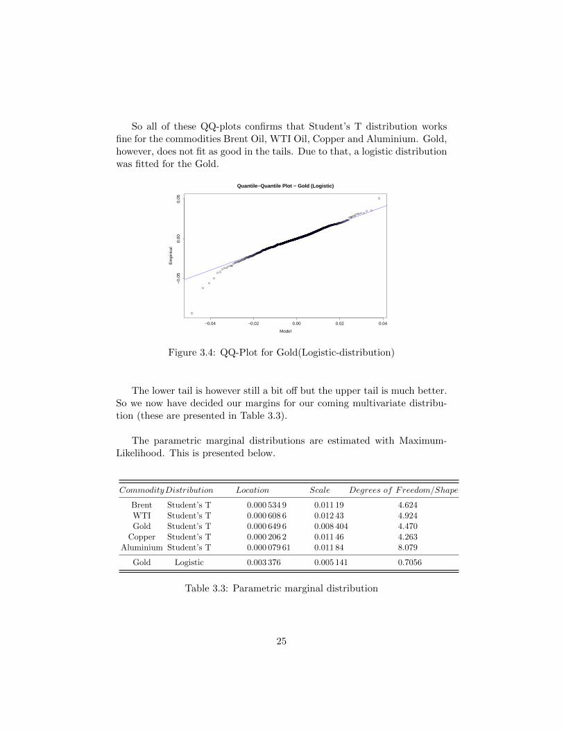
So all of these QQ-plots confirms that Student’s T distribution worksfine for the commodities Brent Oil, WTI Oil, Copper and Aluminium. Gold,however, does not fit as good in the tails. Due to that, a logistic distributionwas fitted for the Gold.

−0.04 −0.02 0.00 0.02 0.04

−0.

050.

000.

05

Quantile−Quantile Plot − Gold (Logistic)

Model

Em

piric

al

Figure 3.4: QQ-Plot for Gold(Logistic-distribution)

The lower tail is however still a bit off but the upper tail is much better.So we now have decided our margins for our coming multivariate distribu-tion (these are presented in Table 3.3).

The parametric marginal distributions are estimated with Maximum-Likelihood. This is presented below.

CommodityDistribution Location Scale Degrees of Freedom/Shape

Brent Student’s T 0.000 534 9 0.011 19 4.624WTI Student’s T 0.000 608 6 0.012 43 4.924Gold Student’s T 0.000 649 6 0.008 404 4.470

Copper Student’s T 0.000 206 2 0.011 46 4.263Aluminium Student’s T 0.000 079 61 0.011 84 8.079

Gold Logistic 0.003 376 0.005 141 0.7056

Table 3.3: Parametric marginal distribution

25

However, to create a multivariate distribution function, we need to es-tablish the dependence between the commodities. Hence, we use Kendall’sTau for this. The Kendall’s Tau for the whole data set (5 years) is presentedbelow.

Kendall′s Brent WTI Gold Copper Aluminium

Brent 1 0.694 884 7 0.194 701 0.283 692 6 0.243 487 8WTI 0.694 884 7 1 0.211 222 1 0.313 573 4 0.287 275 9Gold 0.194 701 0.211 222 1 1 0.261 361 7 0.240 895 8Copper 0.283 692 6 0.313 573 4 0.261 361 7 1 0.514 945 8Aluminium 0.243 487 8 0.287 275 9 0.240 895 8 0.514 945 8 1

Table 3.4: The Kendall’s Tau for the whole five year data set.

Remark: The largest dependence is between Brent Oil and WTI Oil -since they are both oil and fungible commodities.

To decide which copula to use, the Cramer-von Mises method (seeTheory) was used. A wide Goodness-of-Fit test was conducted and theresults are given in Table 3.5 and 3.6 below.

Dimensions Test statistic P − value H0 rejected

2 0.0281 0.005 495 Yes3 0.0347 0.063 44 No4 0.0605 0.003 497 Yes5 0.0595 0.000 499 5 Yes

Table 3.5: Goodness of fit for Normal Copula

where Dimensions are the number of commodities used.

26

Dimensions Test statistic P − value H0 rejected

2 0.0169 0.1304 No3 0.0207 0.5759 No4 0.0335 0.1543 No5 0.0449 0.0415 Yes

Table 3.6: Goodness of fit for T-Copula

In Table 3.6 we can see that the Student’s T Copula was the best up todim = 4 (since p > 0.05 for dim = 2, 3, 4), after that - the p-value is too lowto accept H0.

To counter this problem, we decide to divide the commodities into twogroups where Aluminium is in an own group.

So, the first four commodities (Brent Oil, WTI Oil, Gold and Copper) areconsidered into one group. The same Kendall’s Tau as in table 3:3 is usedto decide the dependence structure(but without the Aluminium part). AStudent’s T Copula is constructed with these dependences using the func-tion tCopula (Please see Theory regarding Student’s T Copula) in R fromthe package Copula. The distributions are then fitted to their respectivedistribution that we found fitting (see Table 3:4). We then use the functionmvdc in R to construct our multivariate distribution function. Finally, wecalculate the probability that the return is less than or equal to 0. Thisis done looking back T number of days (hence constructing a multivariatedistribution function looking back T days.) In our case, a probability plotis constructed looking back 76 days (chosen since it is a bit larger than themean of all T ’s from the PCA part). So the first multivariate distributionfunction uses the data from 76 days - starting on day 1, the second looks atthe 76 days - starting on day 2 and so forth. To explain, when we calculatethe probability from the first 76 days we get a value indicating how big isthe chance that all commodities used are going to have negative or zero re-turn. This means that checking how this develops, we can see which kind of”mood” the market is in at that time - comparing to the other days. Whencan then represent this graphically - see Figure 3:5 below.

27

0 200 400 600 800 1000 1200

0.10

0.15

0.20

0.25

Propability Plot − 4 commodities

Days

Pro

babi

lity

Figure 3.5: Probability Plot that Brent, WTI, Gold and Copper have areturn ≤ 0 when T = 76. This can be seen as a ”indicator” on how thosemarkets are going where a high probability means that the markets are goingdown and a low probability that the markets are supposedly going up.

28

3.5 Part Three - PCA and Copula Combined

To summarize, in the PCA part we use the mean-reversion strategy andthat is then overridden by the momentum strategy. In the Copula part, weuse our results to calculate the probability that the returns for four of ourfive commodities are less than or equal to zero. So what happens when wecombine these parts? Let us find out.

The main idea is that the Copula part should override the two first strategieswhen the probability is large or small enough. Hence, let us try a tradingmodel where we buy all commodities when the probability that the returnsare less than or equal to zero is lower than 0.09 (meanoftheprobabilities−1 standard deviation). And then sell when the probability is higher than0.17 (meanoftheprobabilities + 1 standard deviation). The mean and 1standard deviation is chosen to have a standard reference. This is alsoacting accordingly to the model described in Part Two - Copula above andwith T = 76. With this probabilities, only 197 ∗ 2 = 394 trades were madeout of 1156 (1232− 76 = 1156) possible days. Results are as follows:

Commodity Mean Standard deviation Sharpe Ratio (rf = 0)

Brent −0.045 89 1.511 −0.030 37WTI −0.039 64 1.511 −0.026 23Gold 0.1320 16.17 0.008 166Copper 5.665 122.5 0.046 23

Table 3.7: Test results for copula probability model - selling at P ≥ 0.17

Commodity Mean Standard deviation Sharpe Ratio (rf = 0)

Brent 0.1129 1.460 0.0773WTI 0.1072 1.399 0.076 63Gold 0.4979 15.59 0.031 92Copper −1.655 101.2 −0.016 35

Table 3.8: Test results for copula probability model - buying at P ≤ 0.09

The Sharpe Ratios in total 0.167 which means that it could generatealpha.

29

So, let us combine this with the results that was given in Part One -PCA. We trade all commodities with both mean reversion and momentumwith T and H as presented in Table 3:1. Then the copula part overridesthe trading days where the probability is large or small enough (mean ±standard deviation) for Brent, WTI, Gold and Copper but not Aluminium.Looking at the last 617:1233 trading days we get the following results.

Commodity Mean Standard deviation Sharpe Ratio (rf = 0)

Brent 0.0517 1.2044 0.042 94WTI 0.023 95 1.1980 0.019 99Gold 0.3274 16.05 0.020 39Copper −0.7098 84.03 −0.008 447

Table 3.9: Test results for both PCA and Copula last 617:1233 trading days.

Which gives us a positive total Sharpe Ratio of 0.075.

However, if we include the Aluminium PCA trading part (results of thiscan be found in Table 3:2), we get a total Sharpe Ratio of 0.075− 0.0587 =0.0163.

30

Chapter 4

Discussion

4.1 Summary

The purpose of this master’s thesis was to determine whether PCA andCopula could be used to predict future commodity prices and hence generatealpha. The PCA was used on the first 2.5 years out of 5 years of data to seeif the results could be used on the last half to generate alpha. That could notbe done with our method. Then the returns were fitted to distributions usingMaximum-Likelihood. Student’s T distribution and Logistic distributionwas found to be fitting for the different returns.

Then, the dependence between the commodities was decided using Kendall’sTau.

To decide which copula to use, a Goodness-of-Fit test was conductedusing the Cramer-von Mises method. This showed us that a T-copula couldbe fitted well up to four dimensions.

A probability plot was then constructed based on our dim = 4 T-copulawhere we saw the probability that all first four commodities have a returnless than or equal to zero.

Lastly, the PCA part and the Copula part were combined and a positiveSharpe Ratio was given. However, the low Sharpe Ratio of 0.0163 is not agreat result. This is due to mainly two reasons,

• We have assumed that the risk-free rate rf to be 0 which means thatwe barely are gaining on investing in this prediction model.

• We have not assumed any brokerage fees which must be taken intoaccount since every trade costs - further reducing our positive return.

31

What should be noted is that we have a good result with the PCA partthe first 2.5 years, but those T and H parameters does not provide anyprofit the last 2.5 years. If we had chosen a different criteria for T and H,maybe the model results would have been much better. These values arevery important for the model.

In the description of Maximum Likelihood an assumption is that therandom variables should be i.i.d but this can pretty easily be seen in Figure3:2 that this is not the case. Instead perhaps a GARCH-model could beused to model the observed time series.

Moving on to comment the Copula part - the fitted distributions workedvery well as could be seen in the QQ-plots. Also, the p-values for up todim 4 was very good using T Copula. So why does the model not generatemore alpha? Well, perhaps the way we used our results from the Copulapart should have been used in a different way. Maybe more focus on theCopula part could have given better results. The largest part of the tradingcomes from the PCA part, it would be interesting to see what would happenif the Copula part was the largest part.

Also, it is possible to use the copula distribution in many different ways.Perhaps one could look at expectations or conditional distributions instead.This could have given an even better result and a model which could generatea better Sharpe Ratio.

4.2 Tradeable Results

This thesis does not cover the extra costs that comes with trading suchas hedging, brokerage fees, initial investments(margins) and salaries. Butwith that said, the main purpose to see if we could generate a positive risk-adjusted return with this model is proven.

One should also note that aluminium perhaps was not the best com-modity to exclude in the Copula part. Perhaps gold would be the bestcommodity to exclude since it is a more defensive asset compared to theother commodities used in the thesis. This since investors tend to buy goldwhen the economy is going down as a ”safe harbour”. The other four com-modities used, are more connected to good times in the economy. Hence,gold should maybe have been excluded.

32

The model only covers two alternative states, in a buying mode or in aselling mode. Perhaps a third state should have been introduced where onesimply does nothing. This could have be used in very volatile times whenit is very hard to predict where the market is going. The varying volatilitycan easily be seen when the log-returns are presented in Figure 3:2.

If one looks at this in a larger scale, it is a very narrow field in whichthe investigation was conducted. Nothing says that commodities is the mostpreferred tradeable asset and the model could have been used on assets suchas stocks, foreign exchange or bonds. Another thing to consider is that veryfew commodities were used. If more assets would have been used, maybethe model would be more profitable.

4.3 The Future

Another thing to consider is if it in this case was the optimal solution tooptimize the parameters on the first 2.5 years. Maybe a more continualoptimization would be more fitting. That perhaps one always look back atthe latest year and optimize on that. It would be interesting to see sinceespecially the Copula part shows much promise (the Cramer-von Mises testswere sound up to dim 4).

4.4 Conclusion

To conclude, we can generate a positive risk-adjusted return from this pre-diction model but with a very low Sharpe Ratio.

33

Chapter 5

References

5.1 Reference List

[Banerjee, 2013] Banerjee, J. Origins of Growing Money (January 2015)(Available at forbesindia.com/printcontent/34515)

[Bouye, 2000] Bouye, E (2000) Copulas for Finance A Reading Guide andSome Applications. Financial Econometrics Research Centre, City UniverseBusiness School, London.

[Hull, 2009] John C. Hull (2009) Options, futures and other derivatives.

[Infantino et al., 2010] L.R. Infantino and S.Itzhaki (2010) Developing High-Frequency Equities Trading Models. Massachusetts Institute of Technology.

[Investopedia, 2015] Definition of Mean Reversion (January, 2015).(Available at www.investopedia.com/terms/m/meanreversion.asp)

[Investopedia, 2015] Definition of Sharpe Ratio (January, 2015).(Available at www.investopedia.com/terms/s/sharperatio.asp)

[Jackman, 2009] Jackman, S. (2009) Bayesian Analysis for the Social Sci-ences. Page 507. John Wiley and sons, Ltd

[Jegadeesh et al., 1999] Jegadeesh, N. and Titman, S. Profitiability of Mo-mentum strategies: An evaluation of alternative explanations. NationalBureau of Economic Research, Cambridge MA.

34

[Jolliffe, 2002] Jolliffe, I. T., 2002, Principal Component Analysis, 2nd edi-tion, Springer.

[Krishnamoorthy, 2006] Krishnamoorthy, K. (2006) Handbook of StatisticalDistributions with Applications. Chapman and Hall, Boca Ration, Florida.

[Lutz, 2010] Lutz, B (2010). Pricing of Derivatives on Mean-Reverting As-sets, Chapter 2 - Mean reversion in commodity prices. Springer-VerlagBerlin Heidelberg.

MATLAB Version R2011a

[Myung, 2003] Jae Myung, 2003, Tutorial on maximum likelihood estima-tion, Journal of Mathematical Psychology.

[Nelsen, 2006] Roger B. Nelsen (2006) An Introduction to Copula. Springer

R Package version 1.0-2

[Seber, 2007] George A.F. Seber. (2007) A Matrix Handbook for Statisti-cians. John Wiley and Sons, Inc., Publication

[Shao, 2002] Shao, Q. (2002) Maximum Likelihood Estimation for gener-alised logistic distributions. Marcel Dekker, Inc. New York.

35