for use with simulink - cvut.czradio.feld.cvut.cz/matlab/pdf_doc/rtw/rtw_ug.pdf · for use with...
TRANSCRIPT

Modeling
Simulation
Implementation
Real-Time Workshop®
For Use with Simulink ®
User’s GuideVersion 4
How to Contact The MathWorks:
508-647-7000 Phone
508-647-7001 Fax
The MathWorks, Inc. Mail3 Apple Hill DriveNatick, MA 01760-2098
http://www.mathworks.com Webftp.mathworks.com Anonymous FTP servercomp.soft-sys.matlab Newsgroup
[email protected] Technical [email protected] Product enhancement [email protected] Bug [email protected] Documentation error [email protected] Subscribing user [email protected] Order status, license renewals, [email protected] Sales, pricing, and general information
Real-Time Workshop User’s Guide COPYRIGHT 1994- 2000 by The MathWorks, Inc.The software described in this document is furnished under a license agreement. The software may be usedor copied only under the terms of the license agreement. No part of this manual may be photocopied or repro-duced in any form without prior written consent from The MathWorks, Inc.
FEDERAL ACQUISITION: This provision applies to all acquisitions of the Program and Documentation byor for the federal government of the United States. By accepting delivery of the Program, the governmenthereby agrees that this software qualifies as "commercial" computer software within the meaning of FARPart 12.212, DFARS Part 227.7202-1, DFARS Part 227.7202-3, DFARS Part 252.227-7013, and DFARS Part252.227-7014. The terms and conditions of The MathWorks, Inc. Software License Agreement shall pertainto the government’s use and disclosure of the Program and Documentation, and shall supersede anyconflicting contractual terms or conditions. If this license fails to meet the government’s minimum needs oris inconsistent in any respect with federal procurement law, the government agrees to return the Programand Documentation, unused, to MathWorks.
MATLAB, Simulink, Stateflow, Handle Graphics, and Real-Time Workshop are registered trademarks, andTarget Language Compiler is a trademark of The MathWorks, Inc.
Other product or brand names are trademarks or registered trademarks of their respective holders.
Printing History: May 1994 First printing Version 1January 1998 Second printing Version 2.1January 1999 Third printing Version 3.11 (Release 11)September 2000 Fourth printing Version 4 (Release 12)
i
Contents
Preface
Chapter Summary . . . . . . . . . . . . . . . . . . . . . . . . . . . . . . . . . . . . xvi
Related Products . . . . . . . . . . . . . . . . . . . . . . . . . . . . . . . . . . . . xviii
Installing the Real-Time Workshop . . . . . . . . . . . . . . . . . . . . . xxiThird-Party Compiler Installation on Windows . . . . . . . . . . . xxiiSupported Compilers . . . . . . . . . . . . . . . . . . . . . . . . . . . . . . . . . xxivCompiler Optimization Settings . . . . . . . . . . . . . . . . . . . . . . . . . xxvTypographical Conventions . . . . . . . . . . . . . . . . . . . . . . . . . . . . xxv
1Introduction to the Real-Time Workshop
Product Summary . . . . . . . . . . . . . . . . . . . . . . . . . . . . . . . . . . . . 1-2
Getting Started: Basic Concepts and Tutorials . . . . . . . . . 1-37Tutorial 1: Building a Generic Real-Time Program . . . . . . . . 1-42Tutorial 2: Data Logging . . . . . . . . . . . . . . . . . . . . . . . . . . . . . . 1-49Tutorial 3: Code Validation . . . . . . . . . . . . . . . . . . . . . . . . . . . . 1-52Tutorial 4: A First Look at Generated Code . . . . . . . . . . . . . . 1-56
Where to Find Information in This Manual . . . . . . . . . . . . . 1-63

ii Contents
2Technical Overview
The Rapid Prototyping Process . . . . . . . . . . . . . . . . . . . . . . . . 2-2Key Aspects of Rapid Prototyping . . . . . . . . . . . . . . . . . . . . . . . . 2-2Rapid Prototyping for Digital Signal Processing . . . . . . . . . . . . 2-5Rapid Prototyping for Control Systems . . . . . . . . . . . . . . . . . . . 2-6
Open Architecture of the Real-Time Workshop . . . . . . . . . . 2-8
Automatic Program Building . . . . . . . . . . . . . . . . . . . . . . . . . . 2-12Steps in the Build Process . . . . . . . . . . . . . . . . . . . . . . . . . . . . . 2-13
3Code Generation and the Build Process
Introduction . . . . . . . . . . . . . . . . . . . . . . . . . . . . . . . . . . . . . . . . . . 3-2
Overview of the Real-Time Workshop User Interface . . . . . 3-4Using the Real-Time Workshop Page . . . . . . . . . . . . . . . . . . . . . 3-4Target Configuration Options . . . . . . . . . . . . . . . . . . . . . . . . . . . 3-7General Code Generation Options . . . . . . . . . . . . . . . . . . . . . . . 3-9Target Specific Code Generation Options . . . . . . . . . . . . . . . . . 3-13TLC Debugging Options . . . . . . . . . . . . . . . . . . . . . . . . . . . . . . 3-15Real-Time Workshop Submenu . . . . . . . . . . . . . . . . . . . . . . . . . 3-16
Simulation Parameters and Code Generation . . . . . . . . . . . 3-17Solver Options . . . . . . . . . . . . . . . . . . . . . . . . . . . . . . . . . . . . . . 3-17Workspace I/O Options and Data Logging . . . . . . . . . . . . . . . . 3-18Diagnostics Page Options . . . . . . . . . . . . . . . . . . . . . . . . . . . . . 3-21Advanced Options Page . . . . . . . . . . . . . . . . . . . . . . . . . . . . . . . 3-22Tracing Generated Code Back to YourSimulink Model . . . . . . . . . . . . . . . . . . . . . . . . . . . . . . . . . . . . . 3-28Other Interactions Between Simulinkand the Real-Time Workshop . . . . . . . . . . . . . . . . . . . . . . . . . . 3-29
iii
Selecting a Target Configuration . . . . . . . . . . . . . . . . . . . . . . 3-34The System Target File Browser . . . . . . . . . . . . . . . . . . . . . . . . 3-34Available Targets . . . . . . . . . . . . . . . . . . . . . . . . . . . . . . . . . . . . 3-36
Nonvirtual Subsystem Code Generation . . . . . . . . . . . . . . . . 3-41Nonvirtual Subsystem Code Generation Options . . . . . . . . . . 3-41Modularity of Subsystem Code . . . . . . . . . . . . . . . . . . . . . . . . . 3-48
Generating Code and Executables from Subsystems . . . . . 3-49
Parameters: Storage, Interfacing, and Tuning . . . . . . . . . . 3-51Storage of Nontunable Parameters . . . . . . . . . . . . . . . . . . . . . . 3-51Tunable Parameter Storage . . . . . . . . . . . . . . . . . . . . . . . . . . . 3-53Storage Classes of Tunable Parameters . . . . . . . . . . . . . . . . . . 3-54Using the Model Parameter Configuration Dialog . . . . . . . . . 3-57Tunable Expressions . . . . . . . . . . . . . . . . . . . . . . . . . . . . . . . . . 3-61Tunability of Linear Block Parameters . . . . . . . . . . . . . . . . . . 3-63
Signals: Storage, Optimization, and Interfacing . . . . . . . . . 3-65Signal Storage Concepts . . . . . . . . . . . . . . . . . . . . . . . . . . . . . . 3-65Signals with Auto Storage Class . . . . . . . . . . . . . . . . . . . . . . . . 3-68Declaring Test Points . . . . . . . . . . . . . . . . . . . . . . . . . . . . . . . . . 3-71Interfacing Signals to External Code . . . . . . . . . . . . . . . . . . . . 3-72Symbolic Naming Conventions for Signalsin Generated Code . . . . . . . . . . . . . . . . . . . . . . . . . . . . . . . . . . . 3-74Summary of Signal Storage Class Options . . . . . . . . . . . . . . . . 3-76C API for Parameter Tuning and Signal Monitoring . . . . . . . . 3-77Target Language Compiler API for ParameterTuning and Signal Monitoring . . . . . . . . . . . . . . . . . . . . . . . . . 3-77Parameter Tuning via MATLAB Commands . . . . . . . . . . . . . . 3-77
Simulink Data Objects and Code Generation . . . . . . . . . . . 3-79Prerequisites . . . . . . . . . . . . . . . . . . . . . . . . . . . . . . . . . . . . . . . 3-79Overview . . . . . . . . . . . . . . . . . . . . . . . . . . . . . . . . . . . . . . . . . . . 3-79Parameter Objects . . . . . . . . . . . . . . . . . . . . . . . . . . . . . . . . . . . 3-81Signal Objects . . . . . . . . . . . . . . . . . . . . . . . . . . . . . . . . . . . . . . . 3-85Object Property Information in the model.rtw File . . . . . . . . . 3-88
iv Contents
Configuring the Generated Code via TLC . . . . . . . . . . . . . . 3-93Target Language Compiler Variables and Options . . . . . . . . . 3-93
Making an Executable . . . . . . . . . . . . . . . . . . . . . . . . . . . . . . . . 3-97
Directories Used in the Build Process . . . . . . . . . . . . . . . . . . 3-98
Choosing and Configuring Your Compiler . . . . . . . . . . . . . . 3-99
Template Makefiles and Make Options . . . . . . . . . . . . . . . . 3-102Compiler-Specific Template Makefiles . . . . . . . . . . . . . . . . . . 3-102Template Makefile Structure . . . . . . . . . . . . . . . . . . . . . . . . . 3-106
4Generated Code Formats
Introduction . . . . . . . . . . . . . . . . . . . . . . . . . . . . . . . . . . . . . . . . . . 4-2
Choosing a Code Format for Your Application . . . . . . . . . . . 4-3
Real-Time Code Format . . . . . . . . . . . . . . . . . . . . . . . . . . . . . . . 4-6Unsupported Blocks . . . . . . . . . . . . . . . . . . . . . . . . . . . . . . . . . . . 4-6System Target Files . . . . . . . . . . . . . . . . . . . . . . . . . . . . . . . . . . . 4-6Template Makefiles . . . . . . . . . . . . . . . . . . . . . . . . . . . . . . . . . . . 4-6
Real-Time malloc Code Format . . . . . . . . . . . . . . . . . . . . . . . . . 4-8Unsupported Blocks . . . . . . . . . . . . . . . . . . . . . . . . . . . . . . . . . . . 4-8System Target Files . . . . . . . . . . . . . . . . . . . . . . . . . . . . . . . . . . . 4-8Template Makefiles . . . . . . . . . . . . . . . . . . . . . . . . . . . . . . . . . . . 4-8
S-Function Code Format . . . . . . . . . . . . . . . . . . . . . . . . . . . . . . 4-10
Embedded C Code Format . . . . . . . . . . . . . . . . . . . . . . . . . . . . 4-11
v
5External Mode
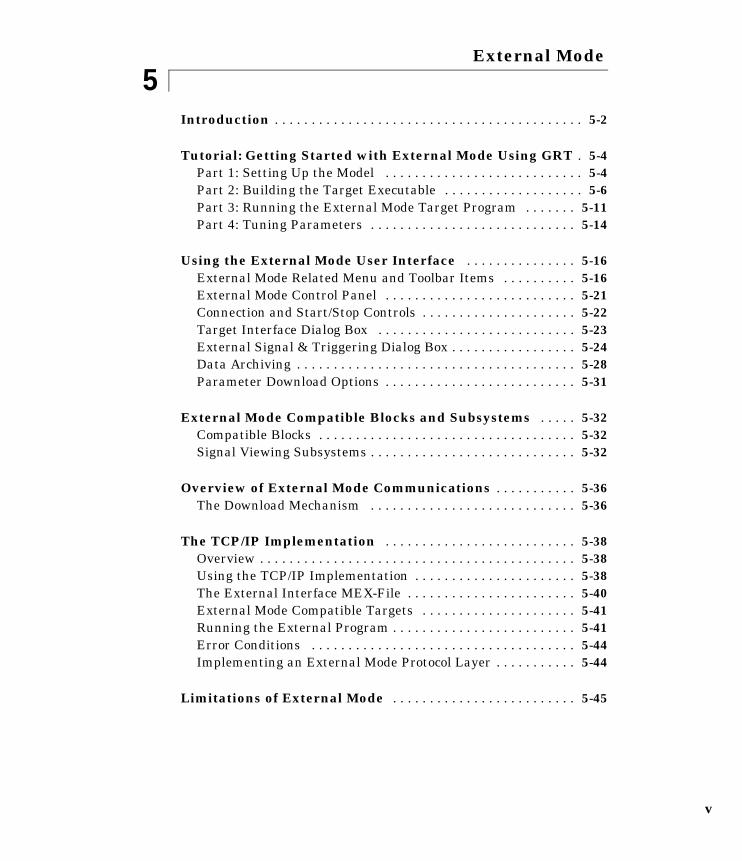
Introduction . . . . . . . . . . . . . . . . . . . . . . . . . . . . . . . . . . . . . . . . . . 5-2
Tutorial: Getting Started with External Mode Using GRT . 5-4Part 1: Setting Up the Model . . . . . . . . . . . . . . . . . . . . . . . . . . . 5-4Part 2: Building the Target Executable . . . . . . . . . . . . . . . . . . . 5-6Part 3: Running the External Mode Target Program . . . . . . . 5-11Part 4: Tuning Parameters . . . . . . . . . . . . . . . . . . . . . . . . . . . . 5-14
Using the External Mode User Interface . . . . . . . . . . . . . . . 5-16External Mode Related Menu and Toolbar Items . . . . . . . . . . 5-16External Mode Control Panel . . . . . . . . . . . . . . . . . . . . . . . . . . 5-21Connection and Start/Stop Controls . . . . . . . . . . . . . . . . . . . . . 5-22Target Interface Dialog Box . . . . . . . . . . . . . . . . . . . . . . . . . . . 5-23External Signal & Triggering Dialog Box . . . . . . . . . . . . . . . . . 5-24Data Archiving . . . . . . . . . . . . . . . . . . . . . . . . . . . . . . . . . . . . . . 5-28Parameter Download Options . . . . . . . . . . . . . . . . . . . . . . . . . . 5-31
External Mode Compatible Blocks and Subsystems . . . . . 5-32Compatible Blocks . . . . . . . . . . . . . . . . . . . . . . . . . . . . . . . . . . . 5-32Signal Viewing Subsystems . . . . . . . . . . . . . . . . . . . . . . . . . . . . 5-32
Overview of External Mode Communications . . . . . . . . . . . 5-36The Download Mechanism . . . . . . . . . . . . . . . . . . . . . . . . . . . . 5-36
The TCP/IP Implementation . . . . . . . . . . . . . . . . . . . . . . . . . . 5-38Overview . . . . . . . . . . . . . . . . . . . . . . . . . . . . . . . . . . . . . . . . . . . 5-38Using the TCP/IP Implementation . . . . . . . . . . . . . . . . . . . . . . 5-38The External Interface MEX-File . . . . . . . . . . . . . . . . . . . . . . . 5-40External Mode Compatible Targets . . . . . . . . . . . . . . . . . . . . . 5-41Running the External Program . . . . . . . . . . . . . . . . . . . . . . . . . 5-41Error Conditions . . . . . . . . . . . . . . . . . . . . . . . . . . . . . . . . . . . . 5-44Implementing an External Mode Protocol Layer . . . . . . . . . . . 5-44
Limitations of External Mode . . . . . . . . . . . . . . . . . . . . . . . . . 5-45
vi Contents
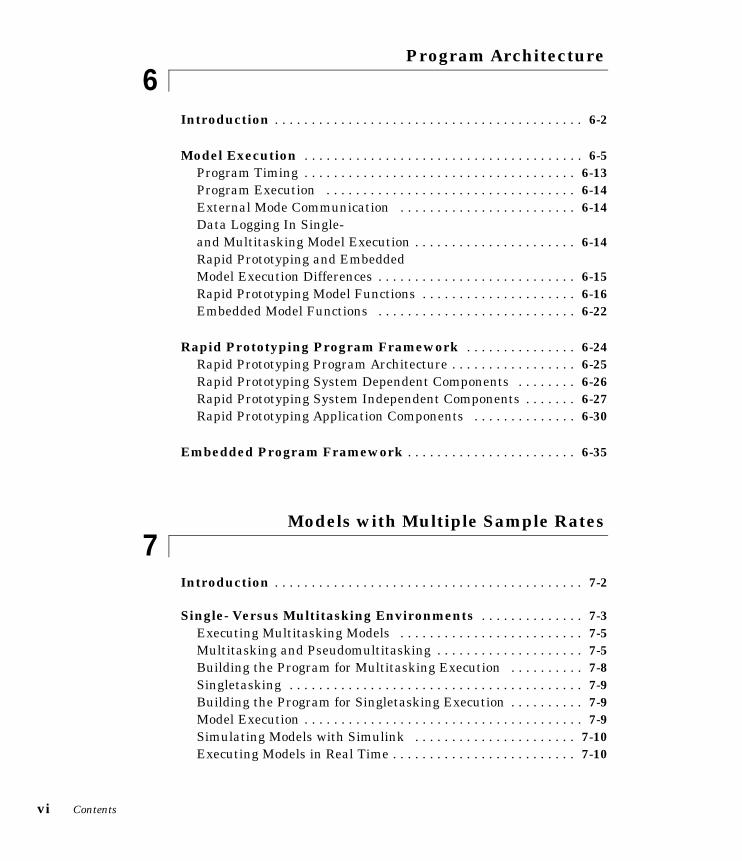
6Program Architecture
Introduction . . . . . . . . . . . . . . . . . . . . . . . . . . . . . . . . . . . . . . . . . . 6-2
Model Execution . . . . . . . . . . . . . . . . . . . . . . . . . . . . . . . . . . . . . . 6-5Program Timing . . . . . . . . . . . . . . . . . . . . . . . . . . . . . . . . . . . . . 6-13Program Execution . . . . . . . . . . . . . . . . . . . . . . . . . . . . . . . . . . 6-14External Mode Communication . . . . . . . . . . . . . . . . . . . . . . . . 6-14Data Logging In Single-and Multitasking Model Execution . . . . . . . . . . . . . . . . . . . . . . 6-14Rapid Prototyping and EmbeddedModel Execution Differences . . . . . . . . . . . . . . . . . . . . . . . . . . . 6-15Rapid Prototyping Model Functions . . . . . . . . . . . . . . . . . . . . . 6-16Embedded Model Functions . . . . . . . . . . . . . . . . . . . . . . . . . . . 6-22
Rapid Prototyping Program Framework . . . . . . . . . . . . . . . 6-24Rapid Prototyping Program Architecture . . . . . . . . . . . . . . . . . 6-25Rapid Prototyping System Dependent Components . . . . . . . . 6-26Rapid Prototyping System Independent Components . . . . . . . 6-27Rapid Prototyping Application Components . . . . . . . . . . . . . . 6-30
Embedded Program Framework . . . . . . . . . . . . . . . . . . . . . . . 6-35
7Models with Multiple Sample Rates
Introduction . . . . . . . . . . . . . . . . . . . . . . . . . . . . . . . . . . . . . . . . . . 7-2
Single- Versus Multitasking Environments . . . . . . . . . . . . . . 7-3Executing Multitasking Models . . . . . . . . . . . . . . . . . . . . . . . . . 7-5Multitasking and Pseudomultitasking . . . . . . . . . . . . . . . . . . . . 7-5Building the Program for Multitasking Execution . . . . . . . . . . 7-8Singletasking . . . . . . . . . . . . . . . . . . . . . . . . . . . . . . . . . . . . . . . . 7-9Building the Program for Singletasking Execution . . . . . . . . . . 7-9Model Execution . . . . . . . . . . . . . . . . . . . . . . . . . . . . . . . . . . . . . . 7-9Simulating Models with Simulink . . . . . . . . . . . . . . . . . . . . . . 7-10Executing Models in Real Time . . . . . . . . . . . . . . . . . . . . . . . . . 7-10

vii
Sample Rate Transitions . . . . . . . . . . . . . . . . . . . . . . . . . . . . . . 7-12Faster to Slower Transitions in Simulink . . . . . . . . . . . . . . . . 7-13Faster to Slower Transitions in Real Time . . . . . . . . . . . . . . . . 7-14Slower to Faster Transitions in Simulink . . . . . . . . . . . . . . . . 7-16Slower to Faster Transitions in Real Time . . . . . . . . . . . . . . . . 7-17
8Optimizing the Model for Code Generation
Overview . . . . . . . . . . . . . . . . . . . . . . . . . . . . . . . . . . . . . . . . . . . . . 8-2
General Modeling Techniques . . . . . . . . . . . . . . . . . . . . . . . . . . 8-3
Block Diagram Performance Tuning . . . . . . . . . . . . . . . . . . . . 8-4Look-Up Tables and Polynomials . . . . . . . . . . . . . . . . . . . . . . . . 8-4Accumulators . . . . . . . . . . . . . . . . . . . . . . . . . . . . . . . . . . . . . . . 8-15Use of Data Types . . . . . . . . . . . . . . . . . . . . . . . . . . . . . . . . . . . 8-17
Stateflow Optimizations . . . . . . . . . . . . . . . . . . . . . . . . . . . . . . 8-23
Simulation Parameters . . . . . . . . . . . . . . . . . . . . . . . . . . . . . . . 8-24
Compiler Options . . . . . . . . . . . . . . . . . . . . . . . . . . . . . . . . . . . . 8-26
9Real-Time Workshop Embedded Coder
Introduction . . . . . . . . . . . . . . . . . . . . . . . . . . . . . . . . . . . . . . . . . . 9-2
Data Structures and Code Modules . . . . . . . . . . . . . . . . . . . . . 9-4Real-Time Object . . . . . . . . . . . . . . . . . . . . . . . . . . . . . . . . . . . . . 9-4Code Modules . . . . . . . . . . . . . . . . . . . . . . . . . . . . . . . . . . . . . . . . 9-5
viii Contents
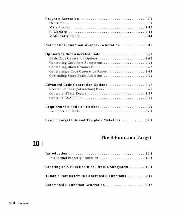
Program Execution . . . . . . . . . . . . . . . . . . . . . . . . . . . . . . . . . . . 9-9Overview . . . . . . . . . . . . . . . . . . . . . . . . . . . . . . . . . . . . . . . . . . . . 9-9Main Program . . . . . . . . . . . . . . . . . . . . . . . . . . . . . . . . . . . . . . 9-10rt_OneStep . . . . . . . . . . . . . . . . . . . . . . . . . . . . . . . . . . . . . . . . . 9-11Model Entry Points . . . . . . . . . . . . . . . . . . . . . . . . . . . . . . . . . . 9-14
Automatic S-Function Wrapper Generation . . . . . . . . . . . . 9-17
Optimizing the Generated Code . . . . . . . . . . . . . . . . . . . . . . . 9-20Basic Code Generation Options . . . . . . . . . . . . . . . . . . . . . . . . . 9-20Generating Code from Subsystems . . . . . . . . . . . . . . . . . . . . . . 9-22Generating Block Comments . . . . . . . . . . . . . . . . . . . . . . . . . . . 9-22Generating a Code Generation Report . . . . . . . . . . . . . . . . . . . 9-23Controlling Stack Space Allocation . . . . . . . . . . . . . . . . . . . . . . 9-25
Advanced Code Generation Options . . . . . . . . . . . . . . . . . . . 9-27Create Simulink (S-Function) Block . . . . . . . . . . . . . . . . . . . . . 9-27Generate HTML Report . . . . . . . . . . . . . . . . . . . . . . . . . . . . . . . 9-27Generate ASAP2 File . . . . . . . . . . . . . . . . . . . . . . . . . . . . . . . . . 9-28
Requirements and Restrictions . . . . . . . . . . . . . . . . . . . . . . . . 9-29Unsupported Blocks . . . . . . . . . . . . . . . . . . . . . . . . . . . . . . . . . . 9-30
System Target File and Template Makefiles . . . . . . . . . . . . 9-31
10The S-Function Target
Introduction . . . . . . . . . . . . . . . . . . . . . . . . . . . . . . . . . . . . . . . . . 10-2Intellectual Property Protection . . . . . . . . . . . . . . . . . . . . . . . . 10-3
Creating an S-Function Block from a Subsystem . . . . . . . . 10-4
Tunable Parameters in Generated S-Functions . . . . . . . . 10-10
Automated S-Function Generation . . . . . . . . . . . . . . . . . . . 10-12
ix
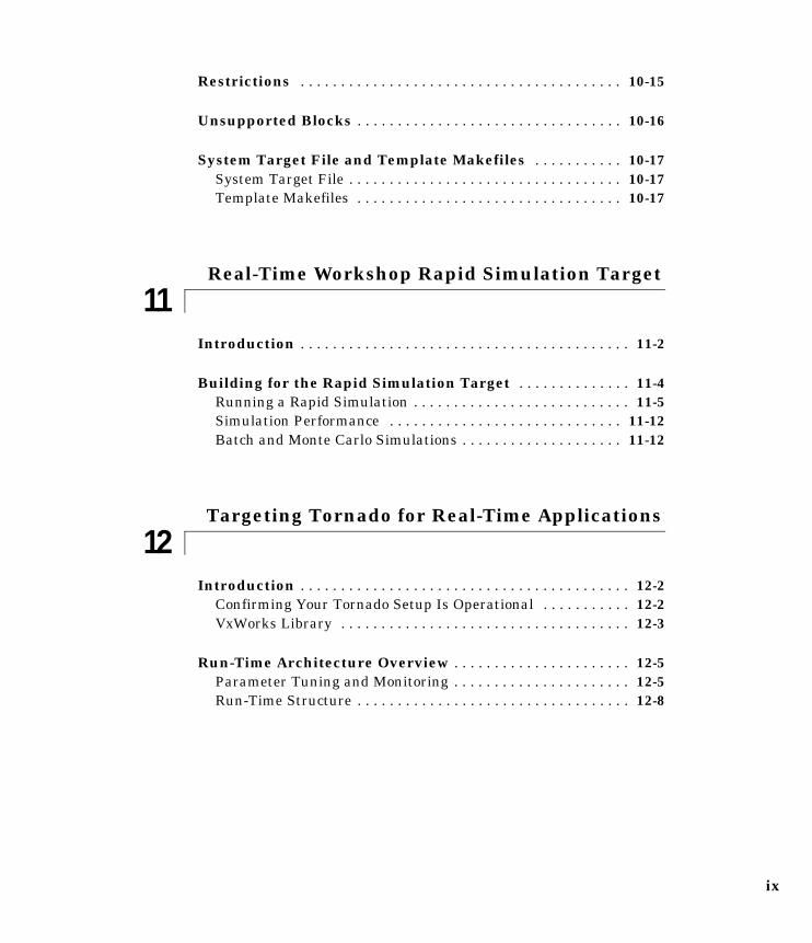
Restrictions . . . . . . . . . . . . . . . . . . . . . . . . . . . . . . . . . . . . . . . . 10-15
Unsupported Blocks . . . . . . . . . . . . . . . . . . . . . . . . . . . . . . . . . 10-16
System Target File and Template Makefiles . . . . . . . . . . . 10-17System Target File . . . . . . . . . . . . . . . . . . . . . . . . . . . . . . . . . . 10-17Template Makefiles . . . . . . . . . . . . . . . . . . . . . . . . . . . . . . . . . 10-17
11Real-Time Workshop Rapid Simulation Target
Introduction . . . . . . . . . . . . . . . . . . . . . . . . . . . . . . . . . . . . . . . . . 11-2
Building for the Rapid Simulation Target . . . . . . . . . . . . . . 11-4Running a Rapid Simulation . . . . . . . . . . . . . . . . . . . . . . . . . . . 11-5Simulation Performance . . . . . . . . . . . . . . . . . . . . . . . . . . . . . 11-12Batch and Monte Carlo Simulations . . . . . . . . . . . . . . . . . . . . 11-12
12Targeting Tornado for Real-Time Applications
Introduction . . . . . . . . . . . . . . . . . . . . . . . . . . . . . . . . . . . . . . . . . 12-2Confirming Your Tornado Setup Is Operational . . . . . . . . . . . 12-2VxWorks Library . . . . . . . . . . . . . . . . . . . . . . . . . . . . . . . . . . . . 12-3
Run-Time Architecture Overview . . . . . . . . . . . . . . . . . . . . . . 12-5Parameter Tuning and Monitoring . . . . . . . . . . . . . . . . . . . . . . 12-5Run-Time Structure . . . . . . . . . . . . . . . . . . . . . . . . . . . . . . . . . . 12-8
x Contents
Implementation Overview . . . . . . . . . . . . . . . . . . . . . . . . . . . 12-12Adding Device Driver Blocks . . . . . . . . . . . . . . . . . . . . . . . . . . 12-14Configuring the Template Makefile . . . . . . . . . . . . . . . . . . . . 12-14Tool Locations . . . . . . . . . . . . . . . . . . . . . . . . . . . . . . . . . . . . . 12-15Building the Program . . . . . . . . . . . . . . . . . . . . . . . . . . . . . . . 12-15Downloading and Running the ExecutableInteractively . . . . . . . . . . . . . . . . . . . . . . . . . . . . . . . . . . . . . . . 12-19
13Targeting DOS for Real-Time Applications
Introduction . . . . . . . . . . . . . . . . . . . . . . . . . . . . . . . . . . . . . . . . . 13-2DOS Device Drivers Library . . . . . . . . . . . . . . . . . . . . . . . . . . . 13-2
Implementation Overview . . . . . . . . . . . . . . . . . . . . . . . . . . . . 13-4System Configuration . . . . . . . . . . . . . . . . . . . . . . . . . . . . . . . . 13-5Sample Rate Limits . . . . . . . . . . . . . . . . . . . . . . . . . . . . . . . . . . 13-7
Device Driver Blocks . . . . . . . . . . . . . . . . . . . . . . . . . . . . . . . . 13-10Device Driver Block Library . . . . . . . . . . . . . . . . . . . . . . . . . . 13-10Configuring Device Driver Blocks . . . . . . . . . . . . . . . . . . . . . . 13-11Adding Device Driver Blocks to the Model . . . . . . . . . . . . . . . 13-16
Building the Program . . . . . . . . . . . . . . . . . . . . . . . . . . . . . . . 13-17Running the Program . . . . . . . . . . . . . . . . . . . . . . . . . . . . . . . 13-18
14Custom Code Blocks
Introduction . . . . . . . . . . . . . . . . . . . . . . . . . . . . . . . . . . . . . . . . . 14-2
Custom Code Library . . . . . . . . . . . . . . . . . . . . . . . . . . . . . . . . . 14-5Model Code Sublibrary . . . . . . . . . . . . . . . . . . . . . . . . . . . . . . . 14-5Subsystem Code Sublibrary . . . . . . . . . . . . . . . . . . . . . . . . . . . 14-9
xi
15Asynchronous Support
Introduction . . . . . . . . . . . . . . . . . . . . . . . . . . . . . . . . . . . . . . . . . 15-2
Interrupt Handling . . . . . . . . . . . . . . . . . . . . . . . . . . . . . . . . . . . 15-5Asynchronous Interrupt Block . . . . . . . . . . . . . . . . . . . . . . . . . 15-5Task Synchronization Block . . . . . . . . . . . . . . . . . . . . . . . . . . 15-12Asynchronous Buffer Block . . . . . . . . . . . . . . . . . . . . . . . . . . . 15-16Rate Transition Block . . . . . . . . . . . . . . . . . . . . . . . . . . . . . . . 15-18
Creating a Customized Asynchronous Library . . . . . . . . . 15-20
16Real-Time Workshop Ada Coder
Introduction . . . . . . . . . . . . . . . . . . . . . . . . . . . . . . . . . . . . . . . . . 16-2Real-Time Workshop Ada Coder Applications . . . . . . . . . . . . . 16-3Supported Compilers . . . . . . . . . . . . . . . . . . . . . . . . . . . . . . . . . 16-3Supported Targets . . . . . . . . . . . . . . . . . . . . . . . . . . . . . . . . . . . 16-3The Generated Code . . . . . . . . . . . . . . . . . . . . . . . . . . . . . . . . . 16-4Types of Output . . . . . . . . . . . . . . . . . . . . . . . . . . . . . . . . . . . . . 16-4Supported Blocks . . . . . . . . . . . . . . . . . . . . . . . . . . . . . . . . . . . . 16-4Restrictions . . . . . . . . . . . . . . . . . . . . . . . . . . . . . . . . . . . . . . . . . 16-4
Getting Started . . . . . . . . . . . . . . . . . . . . . . . . . . . . . . . . . . . . . . 16-6Models with S-Functions . . . . . . . . . . . . . . . . . . . . . . . . . . . . . 16-11Configuring the Template Makefile . . . . . . . . . . . . . . . . . . . . 16-13Data Logging . . . . . . . . . . . . . . . . . . . . . . . . . . . . . . . . . . . . . . 16-13Generating Block Comments . . . . . . . . . . . . . . . . . . . . . . . . . . 16-14Application Modules Required for theReal-Time Program . . . . . . . . . . . . . . . . . . . . . . . . . . . . . . . . . 16-14
Configuring and Interfacing Parameters and Signals . . 16-16Model Parameter Configuration . . . . . . . . . . . . . . . . . . . . . . . 16-16Signal Properties . . . . . . . . . . . . . . . . . . . . . . . . . . . . . . . . . . . 16-16

xii Contents
Code Validation . . . . . . . . . . . . . . . . . . . . . . . . . . . . . . . . . . . . . 16-18Analyzing Data with MATLAB . . . . . . . . . . . . . . . . . . . . . . . . 16-20
Supported Blocks . . . . . . . . . . . . . . . . . . . . . . . . . . . . . . . . . . . 16-21
17Targeting Real-Time Systems
Introduction . . . . . . . . . . . . . . . . . . . . . . . . . . . . . . . . . . . . . . . . . 17-2
Components of a Custom Target Configuration . . . . . . . . . 17-4Code Components . . . . . . . . . . . . . . . . . . . . . . . . . . . . . . . . . . . . 17-4User-Written Run-Time Interface Code . . . . . . . . . . . . . . . . . . 17-5Run-Time Interface for Rapid Prototyping . . . . . . . . . . . . . . . . 17-6Run-Time Interface for Embedded Targets . . . . . . . . . . . . . . . 17-6Control Files . . . . . . . . . . . . . . . . . . . . . . . . . . . . . . . . . . . . . . . . 17-7
Tutorial: Creating a Custom Target Configuration . . . . . . 17-9
Customizing the Build Process . . . . . . . . . . . . . . . . . . . . . . . 17-16System Target File Structure . . . . . . . . . . . . . . . . . . . . . . . . . 17-16Adding a Custom Target to the System TargetFile Browser . . . . . . . . . . . . . . . . . . . . . . . . . . . . . . . . . . . . . . . 17-24Template Makefiles . . . . . . . . . . . . . . . . . . . . . . . . . . . . . . . . . 17-25
Creating Device Drivers . . . . . . . . . . . . . . . . . . . . . . . . . . . . . 17-34Inlined and Noninlined Drivers . . . . . . . . . . . . . . . . . . . . . . . 17-35Device Driver Requirements and Limitations . . . . . . . . . . . . 17-37Parameterizing Your Driver . . . . . . . . . . . . . . . . . . . . . . . . . . 17-38Writing a Noninlined S-Function Device Driver . . . . . . . . . . 17-39Writing an Inlined S-Function Device Driver . . . . . . . . . . . . 17-48Building the MEX-File and the Driver Block . . . . . . . . . . . . . 17-54Source Code for Inlined ADC Driver . . . . . . . . . . . . . . . . . . . . 17-55

xiii
Interfacing Parameters and Signals . . . . . . . . . . . . . . . . . . 17-65Signal Monitoring via Block Outputs . . . . . . . . . . . . . . . . . . . 17-65Parameter Tuning via model_pt.c . . . . . . . . . . . . . . . . . . . . . . 17-71Target Language Compiler API forSignals and Parameters . . . . . . . . . . . . . . . . . . . . . . . . . . . . . . 17-72
Creating an External Mode Communication Channel . . . 17-73The Design of External Mode . . . . . . . . . . . . . . . . . . . . . . . . . 17-73Overview of External Mode Communications . . . . . . . . . . . . 17-74External Mode Source Files . . . . . . . . . . . . . . . . . . . . . . . . . . . 17-76Guidelines for Implementing the Transport Layer . . . . . . . . 17-79
Combining Multiple Models . . . . . . . . . . . . . . . . . . . . . . . . . . 17-82
DSP Processor Support . . . . . . . . . . . . . . . . . . . . . . . . . . . . . . 17-86
ABlocks That Depend on Absolute Time
B Glossary

xiv Contents

Preface
Chapter Summary . . . . . . . . . . . . . . . . . xvi
Related Products . . . . . . . . . . . . . . . . . . xviii
Installing the Real-Time Workshop . . . . . . . . . xxiThird-Party Compiler Installation on Windows . . . . . . xxiiSupported Compilers . . . . . . . . . . . . . . . . . xxivCompiler Optimization Settings . . . . . . . . . . . . xxvTypographical Conventions . . . . . . . . . . . . . . xxv
Preface
xvi
Chapter SummaryChapter 1, “Introduction to the Real-Time Workshop” introduces basicconcepts and terminology of the Real-Time Workshop. It also providesinformation linking basic real-time development tasks to correspondingsections of this book. The “Getting Started: Basic Concepts and Tutorials”section in this chapter will get you working with hands-on exercises.
Chapter 2, “Technical Overview” is a quick introduction to the rapidprototyping process, the open architecture of the Real-Time Workshop, and theautomatic program building process.
Chapter 3, “Code Generation and the Build Process” describes the automaticprogram building process in detail. It discusses all code generation optionscontrolled by the Real-Time Workshop’s graphical user interface. Topicsinclude data logging, inlining and tuning parameters, interfacing parametersand signals to your code, code generation from subsystems, and templatemakefiles. The chapter also summarizes available target configurations.
Chapter 4, “Generated Code Formats” compares and contrasts targets andtheir associated code formats. This include the real-time, real-time malloc,embedded C, and S-Function code formats.
Chapter 5, “External Mode” contains information about external mode, asimulation environment that supports on-the-fly parameter tuning, signalmonitoring, and data logging.
Chapter 6, “Program Architecture” discusses the architecture of programsgenerated by the Real-Time Workshop, and the run-time interface.
Chapter 7, “Models with Multiple Sample Rates” describes how to handlemultirate systems.
Chapter 8, “Optimizing the Model for Code Generation” discusses techniquesfor optimizing your generated programs.
Chapter 9, “Real-Time Workshop Embedded Coder” discusses the structureand operation of programs generated using the Real-Time WorkshopEmbedded Coder. The Real-Time Workshop Embedded Coder is designed forgeneration of code for embedded systems.
Chapter 10, “The S-Function Target” explains how to generate S-Functionblocks from models and subsystems. This enables you to encapsulate modelsand subsystems and protect your designs by distributing only binaries.
Chapter Summary
xvii
Chapter 11, “Real-Time Workshop Rapid Simulation Target” discusses therapid simulation target (RSIM), which executes your model in nonreal-time onyour host computer. You can use this feature to generate fast, stand-alonesimulations that allow batch parameter tuning and the loading of newsimulation data (signals) from a standard MATLAB MAT-file without needingto recompile your model.
Chapter 12, “Targeting Tornado for Real-Time Applications” containsinformation that is specific to developing programs that target Tornado, andsignal monitoring using StethoScope.
Chapter 13, “Targeting DOS for Real-Time Applications” contains informationon developing programs that target DOS.
Chapter 14, “Custom Code Blocks” contains information about the Real-TimeWorkshop library, a collection of blocks and templates you can use to customizecode generation for your application.
Chapter 15, “Asynchronous Support” describes the Interrupt Template library,which allow you to model synchronous/asynchronous event handling.
Chapter 16, “Real-Time Workshop Ada Coder” discusses the Real-TimeWorkshop Ada Target, which generates Ada code from your models. The AdaCoder is a separate product from the Real-Time Workshop.
Chapter 17, “Targeting Real-Time Systems” discusses information of interestto developers who want to develop programs for custom targets. This includesdeveloping device driver blocks, customizing system target files and templatemakefiles, combining multiple models into a single executable, and APIs forexternal mode communication, signal monitoring, and parameter tuning.
Appendix A lists blocks whose use is restricted due to dependency on absolutetime.
Appendix B is a glossary that contains definitions of terminology associatedwith the Real-Time Workshop and real-time development.

Preface
xviii
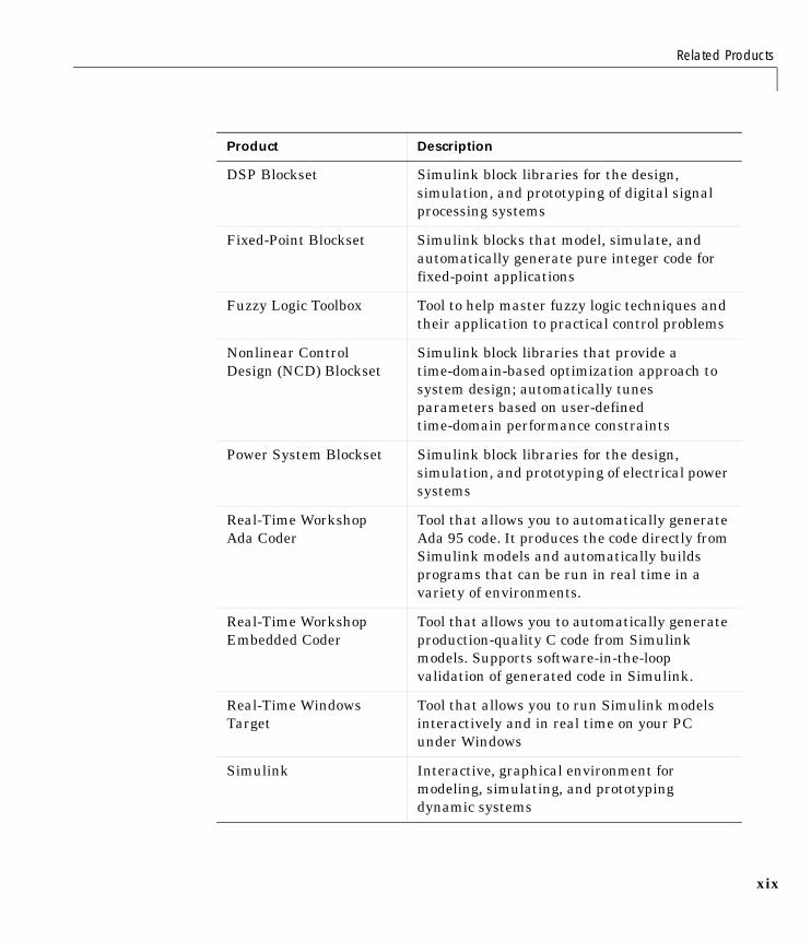
Related ProductsThe MathWorks provides several products that are especially relevant to thekinds of tasks you can perform with the Real-Time Workshop®. They are listedin the table below.
The Real-Time Workshop requires these products:
• MATLAB® 6.0 (Release 12)
• Simulink® 4.0 (Release 12)
• A supported compiler (See “Supported Compilers” on page xxiv and“Third-Party Compiler Installation on Windows” on page xxii)
For more information about any of these products, see either:
• The online documentation for that product, if it is installed or if you arereading the documentation from the CD
• The MathWorks Web site, at http://www.mathworks.com; see the “products”section
Note The toolboxes listed below all include functions that extend MATLAB’scapabilities. The blocksets listed below all include blocks that extendSimulink’s capabilities.
Product Description
Communications Toolbox MATLAB functions for modeling the physicallayer of communications systems
Control System Toolbox Tool for modeling, analyzing, and designingcontrol systems using classical and moderntechniques
Dials & Gauges Blockset Graphical instrumentation for monitoring andcontrolling signals and parameters inSimulink models
Related Products
xix
DSP Blockset Simulink block libraries for the design,simulation, and prototyping of digital signalprocessing systems
Fixed-Point Blockset Simulink blocks that model, simulate, andautomatically generate pure integer code forfixed-point applications
Fuzzy Logic Toolbox Tool to help master fuzzy logic techniques andtheir application to practical control problems
Nonlinear ControlDesign (NCD) Blockset
Simulink block libraries that provide atime-domain-based optimization approach tosystem design; automatically tunesparameters based on user-definedtime-domain performance constraints
Power System Blockset Simulink block libraries for the design,simulation, and prototyping of electrical powersystems
Real-Time WorkshopAda Coder
Tool that allows you to automatically generateAda 95 code. It produces the code directly fromSimulink models and automatically buildsprograms that can be run in real time in avariety of environments.
Real-Time WorkshopEmbedded Coder
Tool that allows you to automatically generateproduction-quality C code from Simulinkmodels. Supports software-in-the-loopvalidation of generated code in Simulink.
Real-Time WindowsTarget
Tool that allows you to run Simulink modelsinteractively and in real time on your PCunder Windows
Simulink Interactive, graphical environment formodeling, simulating, and prototypingdynamic systems
Product Description

Preface
xx
Stateflow® Tool for graphical modeling and simulation ofcomplex control logic
Stateflow Coder Tool for generating highly readable, efficient Ccode from Stateflow diagrams
xPC Target Tool that supports many I/O blocks forSimulink block diagrams. Supportsdownloading code generated by Real-TimeWorkshop to a second PC that runs the xPCTarget real-time kernel, for rapid prototypingand hardware-in-the-loop testing of controland DSP systems.
xPC Target EmbeddedOption
Add-on to xPC Target to deploy the xPC Targetoperating system, together with embeddedcode, to external PCs
Product Description

Installing the Real-Time Workshop
xxi
Installing the Real-Time WorkshopYour platform-specific MATLAB Installation Guide provides all of theinformation you need to install the Real-Time Workshop.
Prior to installing the Real-Time Workshop, you must obtain a License File orPersonal License Password from The MathWorks. The License File or PersonalLicense Password identifies the products you are permitted to install and use.
As the installation process proceeds, it displays a dialog similar to the onebelow, letting you indicate which products to install.
Preface
xxii
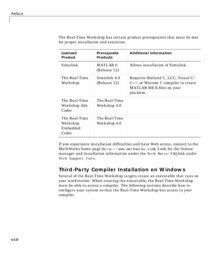
The Real-Time Workshop has certain product prerequisites that must be metfor proper installation and execution.
If you experience installation difficulties and have Web access, connect to theMathWorks home page (http://www.mathworks.com). Look for the licensemanager and installation information under the Tech Notes/FAQ link underTech Support Info.
Third-Party Compiler Installation on WindowsSeveral of the Real-Time Workshop targets create an executable that runs onyour workstation. When creating the executable, the Real-Time Workshopmust be able to access a compiler. The following sections describe how toconfigure your system so that the Real-Time Workshop has access to yourcompiler.
Licensed Product
Prerequisite Products
Additional Information
Simulink MATLAB 6(Release 12)
Allows installation of Simulink.
The Real-TimeWorkshop
Simulink 4.0(Release 12)
Requires Borland C, LCC, Visual C/C++, or Watcom C compiler to createMATLAB MEX-files on yourplatform.
The Real-TimeWorkshop AdaCoder
The Real-TimeWorkshop 4.0
The Real-TimeWorkshopEmbeddedCoder
The Real-TimeWorkshop 4.0

Installing the Real-Time Workshop
xxiii
Borland Make sure that your Borland environment variable is defined and correctlypoints to the directory in which your Borland compiler resides. To check this,type
set BORLAND
at the DOS prompt. The return from this includes the selected directory.
If the BORLAND environment variable is not defined, you must define it to pointto where you installed your Borland compiler. On Microsoft Windows 95 or 98,add
set BORLAND=<path to your compiler>
to your autoexec.bat file.
On Microsoft Windows NT, in the control panel select System, go to theEnvironment page, and define BORLAND to be the path to your compiler.
LCCThe freeware LCC C compiler is shipped with MATLAB, and is installed withthe product. If you want to use LCC to build programs generated by theReal-Time Workshop, you should use the version that is currently shipped withthe product. Information about LCC is available athttp://www.cs.virginia.edu/~lcc-win32/.
Microsoft Visual C/C++Define the environment variable MSDevDir to be
MSDevDir=<path to compiler>\SharedIDE for Visual C/C++ 5.0MSDevDir=<path to compiler>\Common\MSDev98 for Visual C/C++ 6.0
Watcom
Note As of this printing, the Watcom C compiler is no longer available fromthe manufacturer. The Real-Time Workshop continues to ship Watcom-relatedtarget configurations at this time. However, this policy may be subject tochange in the future.

Preface
xxiv
Make sure that your Watcom environment variable is defined and correctlypoints to the directory in which your Watcom compiler resides. To check this,type
set WATCOM
at the DOS prompt. The return from this includes the selected directory.
If the WATCOM environment variable is not defined, you must define it to pointto where you installed your Watcom compiler. On Windows 95 or 98, add
set WATCOM=<path to your compiler>
to your autoexec.bat file.
On Windows NT, in the control panel select System, go to the Environmentpage, and define WATCOM to be the path to your compiler.
Out-of-Environment Error MessageIf you are receiving out-of-environment space error messages, you canright-click your mouse on the program that is causing the problem (forexample, dosprmpt or autoexec.bat) and choose Properties. From therechoose Memory. Set the Initial Environment to the maximum allowed andclick Apply. This should increase the amount of environment space available.
Supported Compilers
On Windows. As of this printing, we have tested the Real-Time Workshop withthese compilers on Windows.
Compiler Versions
Borland 5.3, 5.4,5.5
LCC Use version of LCC shipped withMATLAB.
Microsoft Visual C/C++ 5.0, 6.0
Watcom 10.6, 11.0 (see “Watcom” above)
Installing the Real-Time Workshop
xxv
Typically you must make modifications to your setup when a new version ofyour compiler is released. See the MathWorks home page,http://www.mathworks.com, for up-to-date information on newer compilers.
On UNIX. On UNIX, the Real-Time Workshop build process uses the defaultcompiler. cc is the default on all platforms except SunOS, where gcc is thedefault.
Compiler Optimization SettingsIn some very rare instances, due to compiler defects, compiler optimizationsapplied to Real-Time Workshop generated code may cause the executableprogram to produce incorrect results, even though the code itself is correct.
The Real-Time Workshop uses the default optimization level for supportedcompilers. You can usually work around problems caused by compileroptimizations by lowering the optimization level of the compiler, or turning offoptimizations. Please refer to your compiler's documentation for informationon how to do this.
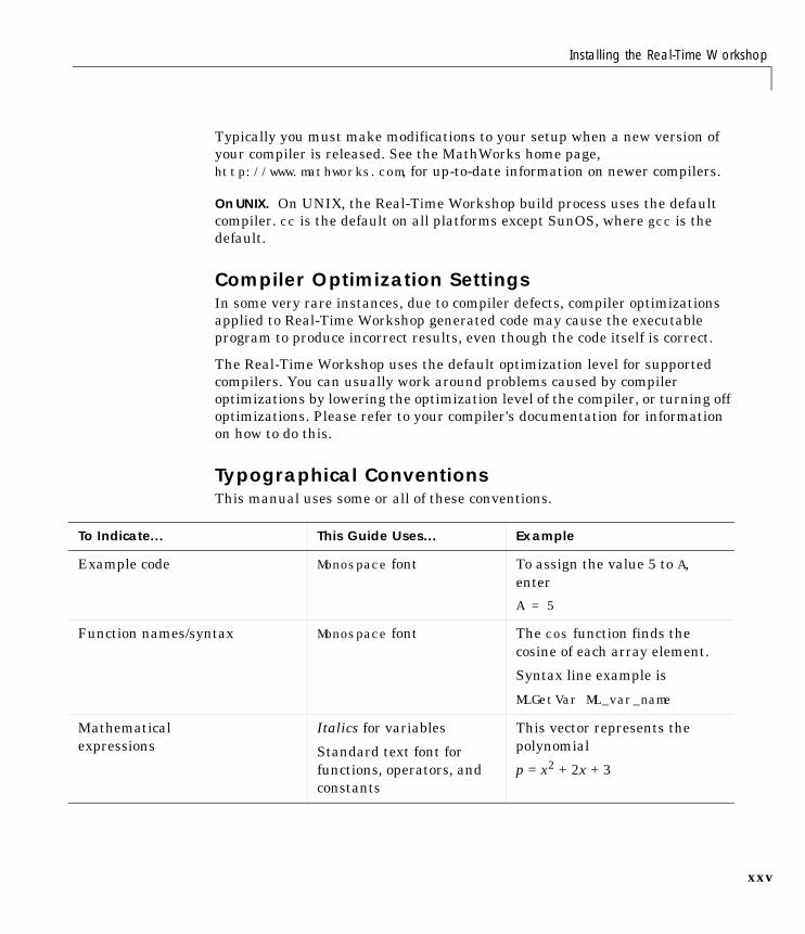
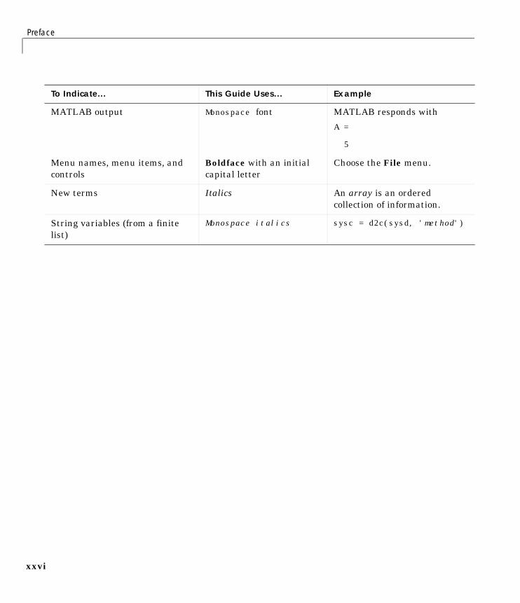
Typographical ConventionsThis manual uses some or all of these conventions.
To Indicate... This Guide Uses... Example
Example code Monospace font To assign the value 5 to A,enter
A = 5
Function names/syntax Monospace font The cos function finds thecosine of each array element.
Syntax line example is
MLGetVar ML_var_name
Mathematicalexpressions
Italics for variables
Standard text font forfunctions, operators, andconstants
This vector represents thepolynomial
p = x2 + 2x + 3
Preface
xxvi
MATLAB output Monospace font MATLAB responds with
A =
5
Menu names, menu items, andcontrols
Boldface with an initialcapital letter
Choose the File menu.
New terms Italics An array is an orderedcollection of information.
String variables (from a finitelist)
Monospace italics sysc = d2c(sysd, 'method')
To Indicate... This Guide Uses... Example
1Introduction to theReal-Time Workshop
Product Summary . . . . . . . . . . . . . . . . . 1-2
Getting Started: Basic Concepts and Tutorials . . . . 1-37Tutorial 1: Building a Generic Real-Time Program . . . . . 1-42Tutorial 2: Data Logging . . . . . . . . . . . . . . . 1-49Tutorial 3: Code Validation . . . . . . . . . . . . . . 1-52Tutorial 4: A First Look at Generated Code . . . . . . . . 1-56
Where to Find Information in This Manual . . . . . . 1-63
1 Introduction to the Real-Time Workshop
1-2
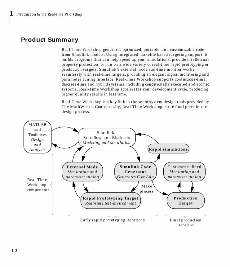
Product SummaryReal-Time Workshop generates optimized, portable, and customizable codefrom Simulink models. Using integrated makefile based targeting support, itbuilds programs that can help speed up your simulations, provide intellectualproperty protection, or run on a wide variety of real-time rapid prototyping orproduction targets. Simulink’s external mode run-time monitor worksseamlessly with real-time targets, providing an elegant signal monitoring andparameter tuning interface. Real-Time Workshop supports continuous-time,discrete-time and hybrid systems, including conditionally executed and atomicsystems. Real-Time Workshop accelerates your development cycle, producinghigher quality results in less time.
Real-Time Workshop is a key link in the set of system design tools provided byThe MathWorks. Conceptually, Real-Time Workshop is the final piece in thedesign process.
Simulink,
Modeling and simulationStateflow, and Blocksets
External ModeMonitoring and
parameter tuning
Simulink CodeGenerator
Generates C or Ada
ProductionTarget
MATLABand
ToolboxesDesign
andAnalysis
Customer definedMonitoring and
parameter tuning
Early rapid prototyping iterations Final productioniteration
Real-TimeWorkshopcomponents
Rapid simulations
Makeprocess
Rapid Prototyping TargetReal-time test environment

Product Summary
1-3
Real-Time Workshop provides a real-time development environment — adirect path from system design to hardware implementation. You can shortendevelopment cycles and reduce costs with Real-Time Workshop by testingdesign iterations with real-time hardware. Real-Time Workshop supports theexecution of dynamic system models on hardware by automatically convertingmodels to code and providing model-based debugging support. It is well suitedfor accelerating simulations, rapid prototyping, turnkey solutions, andproduction embedded real-time applications.
With Real-Time Workshop, you can quickly generate C code for discrete-time,continuous-time, and hybrid systems, including systems containing triggeredand enabled subsystems. With the optional Real-Time Workshop Ada Coder,you can generate Ada code. The optional Stateflow Coder add-on lets yougenerate code for finite state machines modeled in Stateflow.
System design using the MathWorks toolset differs from one application toanother. A typical product cycle starts with modeling in Simulink, followed byan analysis of the simulations in MATLAB. During the simulation process, youuse the rapid simulation features of Real-Time Workshop to speed up yoursimulations.
After you are satisfied with the simulation results, you use Real-TimeWorkshop in conjunction with a rapid prototyping target, such as xPC Target.The rapid prototyping target is connected to your physical system. You test andobserve your system, using your Simulink model as the interface to yourphysical target. After creating your model, you use Real-Time Workshop totransform your model to C or Ada code. An extensible make process anddownload procedure creates an executable for your model and places it on thetarget system. Finally, using external mode, you can monitor and tuneparameters in real-time as your model executes on the target environment.
Conceptually, there are two types of targets: rapid prototyping targets and theembedded target. Code generated for the rapid prototyping targets supportsincreased monitoring and tuning capabilities. The generated embedded codeused in the embedded target is highly optimized and suitable for deploymentin production systems. You can add application-specific entry points to monitorsignals and tune parameters in the embedded code.
1 Introduction to the Real-Time Workshop
1-4
The basic components of Real-Time Workshop are:
• Simulink Code Generator: automatically generates C or Ada code from yourSimulink model.
• Make Process: The Real-Time Workshop’s user-extensible make process letsyou create your own production or rapid prototyping target.
• Simulink External Mode: External mode enables communication betweenSimulink and a model executing on a real-time test environment, or inanother process on the same machine. External mode lets you performreal-time parameter tuning and data viewing using Simulink as a front end.
• Targeting Support: Using Real-Time Workshop’s bundled targets, you canbuild systems for a number of environments, including Tornado and DOS.The generic real-time and embedded real-time targets provide a frameworkfor developing customized rapid prototyping or production targetenvironments. In addition to the bundled targets, Real-Time WindowsTarget and/or xPC Target let you turn a PC of any form factor into a rapidprototyping target, or a small to medium volume production target.
• Rapid Simulations: Using Simulink Accelerator (part of the SimulinkPerformance Tools product), S-Function Target, or Rapid Simulation Target,you can accelerate your simulations by 5 to 20 times on average. Executablesbuilt with these targets bypass Simulink’s normal interpretive simulationmode, which must handle all configurations of each basic modeling primitive.The code generated by Simulink Accelerator, S-Function Target, or RapidSimulation Target is highly optimized to execute only the algorithms used inyour specific model. In addition, these targets apply many optimizations,such as eliminating ones and zeros in computations for filter blocks.
Integrated Development EnvironmentIf the Real-Time Workshop target you are using supports Simulink externalmode, you can use Simulink as the monitoring/debugging interface for thegenerated code. With external mode, you can:
• Change parameters via the block dialogs, gauges, and the set_paramMATLAB command. The set_param command lets you interactprogrammatically with your target.
• View target signals in Scope blocks, Display blocks, general S-Functionblocks, and via gauges.
Product Summary
1-5
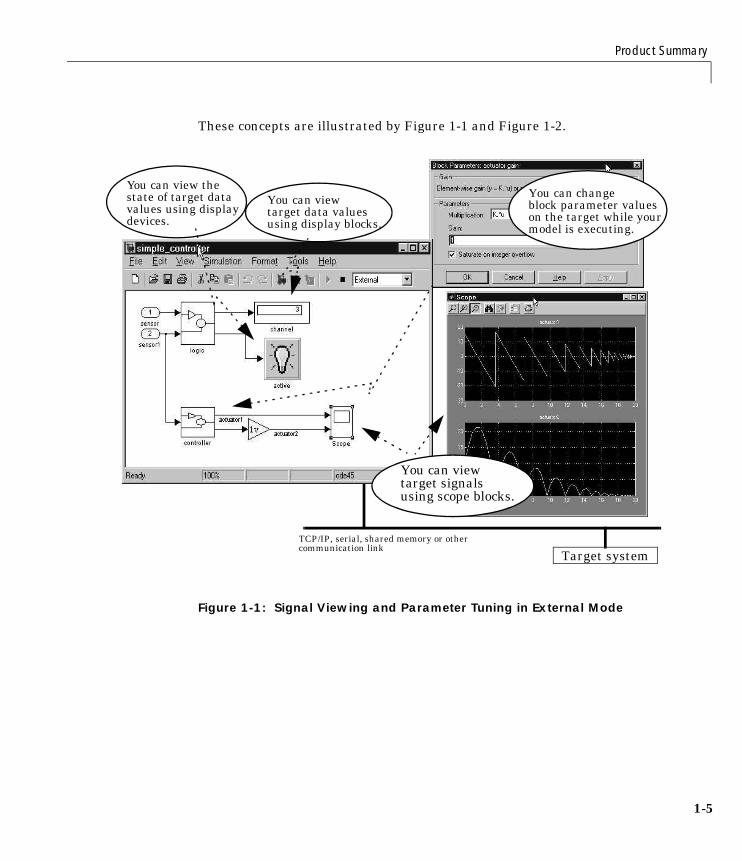
These concepts are illustrated by Figure 1-1 and Figure 1-2.
Figure 1-1: Signal Viewing and Parameter Tuning in External Mode
Target systemTCP/IP, serial, shared memory or othercommunication link
You can changeblock parameter valueson the target while yourmodel is executing.
You can viewtarget data valuesusing display blocks.
You can view thestate of target datavalues using displaydevices.
You can viewtarget signalsusing scope blocks.
1 Introduction to the Real-Time Workshop
1-6
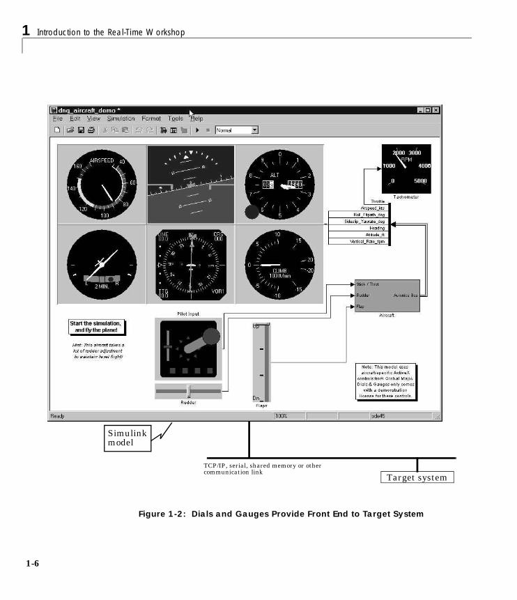
Figure 1-2: Dials and Gauges Provide Front End to Target System
Simulinkmodel
Target systemTCP/IP, serial, shared memory or othercommunication link
Product Summary
1-7
A Next-Generation Development ToolThe MathWorks toolset, including Simulink and Real-Time Workshop, isrevolutionizing the way embedded systems are designed. Simulink is a veryhigh level language (VHLL) — a next-generation programing language. A brieflook at the history of dynamic and embedded system design methodologiesreveals a steady progression toward higher-level design tools and processes:
• Design -> analog components: Before the introduction of microcontrollers,design was done on paper and realized using analog components.
• Design -> hand written assembly -> early microcontrollers: In the earlymicroprocessor era, design was done on paper and realized by writingassembly code and placing it on microcontrollers. Today, very low-endapplications still use assembly language, but advancements in Real-TimeWorkshop and C/Ada compiler technology will soon render such techniquesobsolete.
• Design -> high-level language (HLL) -> object code -> microcontroller: Theadvent of efficient HLL compilers led to the realization of paper designs inlanguages such as C. HLL code, transformed to assembly language by acompiler, was then placed on a microcontroller. In the early days ofhigh-level languages, programmers often inspected the machine generatedassembly code produced by compilers for correctness. Today, it is taken forgranted that the assembly code is correct.
• Design -> modeling tool -> manual HLL coding -> object code ->microcontroller: When design tools such as Simulink appeared, designerswere able to express system designs graphically and simulate them forcorrectness. While this process saved considerable time and improvedperformance, designs were still translated to C code manually before beingplaced on a microcontroller. This translation process was both timeconsuming and error prone.
• Design -> Simulink -> Real-Time Workshop (automatic code generation) ->object code -> microcontroller. With the addition of Real-Time Workshop,Simulink itself becomes a very high level language (VHLL). Modelingconstructs in Simulink are the basic elements of the language. TheReal-Time Workshop then compiles models to produce C or Ada code. Thismachine-generated code is produced quickly and correctly. The manual
1 Introduction to the Real-Time Workshop
1-8
process of transforming designs to code has now been eliminated, yieldingsignificant improvements in system design.
The Simulink code generator included within Real-Time Workshop is anext-generation graphical block diagram compiler. Real-Time Workshop hascapabilities beyond those of a typical HLL compiler. Generated code is highlyreadable and customizable. It is normally unnecessary to read the object codeproduced by the HLL compiler.. You can use the Real-Time Workshop in awide variety of applications, improving your design process.
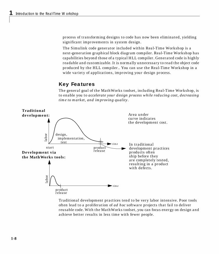
Key FeaturesThe general goal of the MathWorks toolset, including Real-Time Workshop, isto enable you to accelerate your design process while reducing cost, decreasingtime to market, and improving quality.
Traditional development practices tend to be very labor intensive. Poor toolsoften lead to a proliferation of ad hoc software projects that fail to deliverreusable code. With the MathWorks toolset, you can focus energy on design andachieve better results in less time with fewer people.
labo
r
start
design,implementation,
product
test
release
Traditionaldevelopment:
time
time
Development viathe MathWorks tools:
productrelease
labo
r
Area undercurve indicatesthe development cost.
In traditionaldevelopment practicesproducts oftenship before theyare completely tested,resulting in a productwith defects.
Product Summary
1-9
Real-Time Workshop, along with other components of the MathWorks tools,provides:
• A rapid and direct path from system design to implementation
• Seamless integration with MATLAB and Simulink
• A simple graphical user interface
• An open and extensible architecture
The following features of Real-Time Workshop enable you to reach the abovegoal:
• Code generator for Simulink models- Generates optimized, customizable code. There are several styles of
generated code, which can be classified as either embedded (productionphase) or rapid prototyping.
- Supports all Simulink features, including 8, 16, and 32 bit integers andfloating-point data types.
- Fixed-Point Blockset and Real-Time Workshop allow for scaling of integerwords ranging from 2 to 128 bits. Code generation is limited by theimplementation of char, short, int, and long in embedded C compilerenvironments (usually 8, 16, and 32 bits).
- Generated code is processor independent. The generated code representsyour model exactly. A separate run-time interface is used to execute thiscode. We provide several example run-time interfaces as well asproduction run-time interfaces.
- Supports any single or multitasking operating system. Also supports“bare-board” (no operating system) environments.
- The Target Language CompilerTM (TLC) allows extensive customization ofthe generated code.
- Provides for custom code generation for S-functions (user-created blocks)via TLC, enabling you to embed very efficient custom code into the model’sgenerated code.
• Extensive model-based debugging support- External mode enables you to examine what the generated code is doing
by uploading data from your target to the graphical display elements inyour model. There is no need to use a conventional C or Ada debugger tolook at your generated code.
1 Introduction to the Real-Time Workshop
1-10
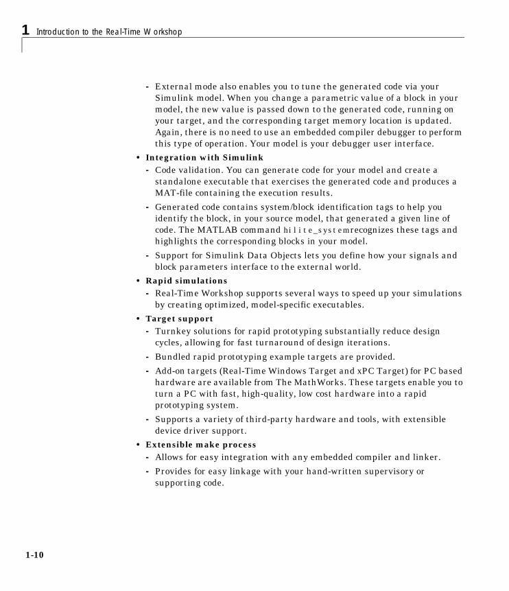
- External mode also enables you to tune the generated code via yourSimulink model. When you change a parametric value of a block in yourmodel, the new value is passed down to the generated code, running onyour target, and the corresponding target memory location is updated.Again, there is no need to use an embedded compiler debugger to performthis type of operation. Your model is your debugger user interface.
• Integration with Simulink- Code validation. You can generate code for your model and create a
standalone executable that exercises the generated code and produces aMAT-file containing the execution results.
- Generated code contains system/block identification tags to help youidentify the block, in your source model, that generated a given line ofcode. The MATLAB command hilite_system recognizes these tags andhighlights the corresponding blocks in your model.
- Support for Simulink Data Objects lets you define how your signals andblock parameters interface to the external world.
• Rapid simulations- Real-Time Workshop supports several ways to speed up your simulations
by creating optimized, model-specific executables.• Target support
- Turnkey solutions for rapid prototyping substantially reduce designcycles, allowing for fast turnaround of design iterations.
- Bundled rapid prototyping example targets are provided.
- Add-on targets (Real-Time Windows Target and xPC Target) for PC basedhardware are available from The MathWorks. These targets enable you toturn a PC with fast, high-quality, low cost hardware into a rapidprototyping system.
- Supports a variety of third-party hardware and tools, with extensibledevice driver support.
• Extensible make process- Allows for easy integration with any embedded compiler and linker.
- Provides for easy linkage with your hand-written supervisory orsupporting code.
Product Summary
1-11
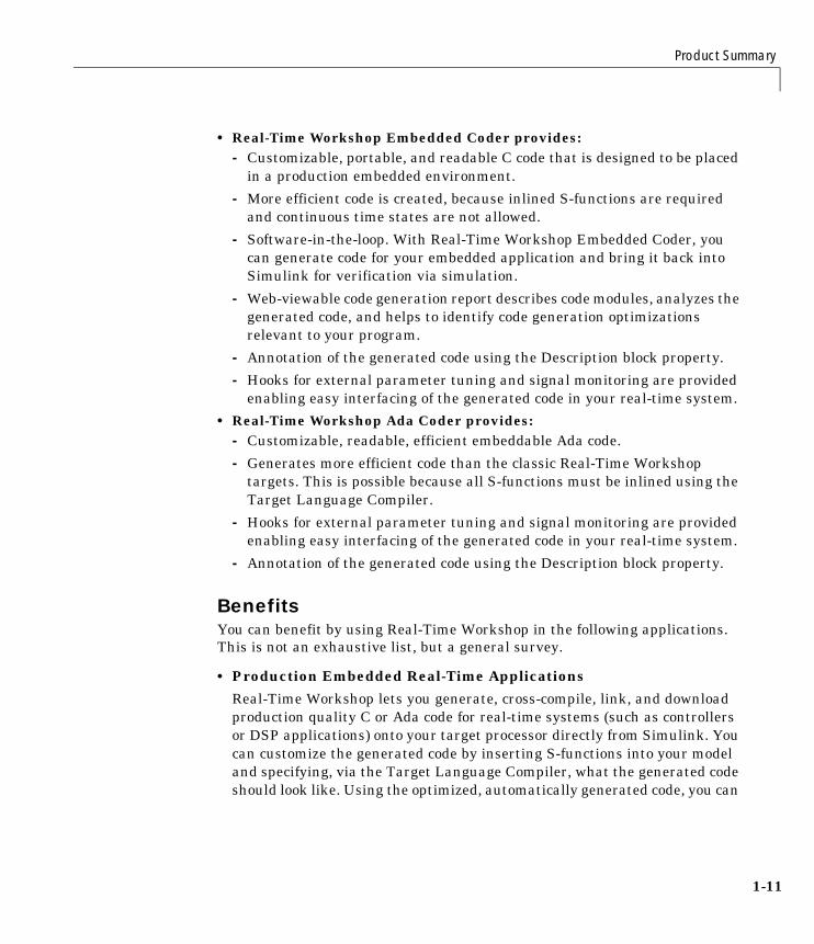
• Real-Time Workshop Embedded Coder provides:- Customizable, portable, and readable C code that is designed to be placed
in a production embedded environment.
- More efficient code is created, because inlined S-functions are requiredand continuous time states are not allowed.
- Software-in-the-loop. With Real-Time Workshop Embedded Coder, youcan generate code for your embedded application and bring it back intoSimulink for verification via simulation.
- Web-viewable code generation report describes code modules, analyzes thegenerated code, and helps to identify code generation optimizationsrelevant to your program.
- Annotation of the generated code using the Description block property.
- Hooks for external parameter tuning and signal monitoring are providedenabling easy interfacing of the generated code in your real-time system.
• Real-Time Workshop Ada Coder provides:- Customizable, readable, efficient embeddable Ada code.
- Generates more efficient code than the classic Real-Time Workshoptargets. This is possible because all S-functions must be inlined using theTarget Language Compiler.
- Hooks for external parameter tuning and signal monitoring are providedenabling easy interfacing of the generated code in your real-time system.
- Annotation of the generated code using the Description block property.
BenefitsYou can benefit by using Real-Time Workshop in the following applications.This is not an exhaustive list, but a general survey.
• Production Embedded Real-Time Applications
Real-Time Workshop lets you generate, cross-compile, link, and downloadproduction quality C or Ada code for real-time systems (such as controllersor DSP applications) onto your target processor directly from Simulink. Youcan customize the generated code by inserting S-functions into your modeland specifying, via the Target Language Compiler, what the generated codeshould look like. Using the optimized, automatically generated code, you can
1 Introduction to the Real-Time Workshop
1-12
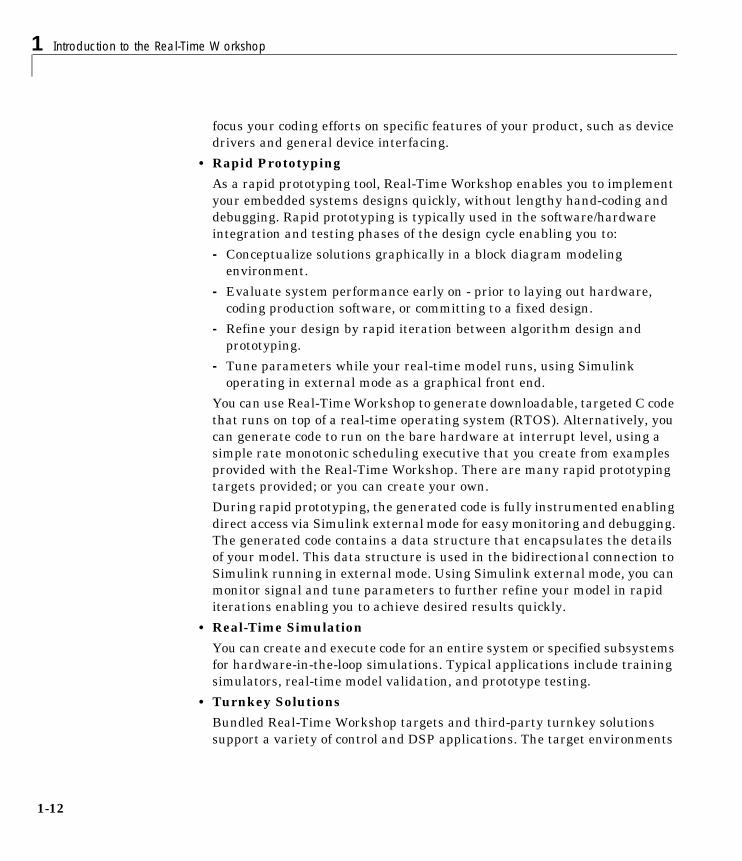
focus your coding efforts on specific features of your product, such as devicedrivers and general device interfacing.
• Rapid Prototyping
As a rapid prototyping tool, Real-Time Workshop enables you to implementyour embedded systems designs quickly, without lengthy hand-coding anddebugging. Rapid prototyping is typically used in the software/hardwareintegration and testing phases of the design cycle enabling you to:
- Conceptualize solutions graphically in a block diagram modelingenvironment.
- Evaluate system performance early on - prior to laying out hardware,coding production software, or committing to a fixed design.
- Refine your design by rapid iteration between algorithm design andprototyping.
- Tune parameters while your real-time model runs, using Simulinkoperating in external mode as a graphical front end.
You can use Real-Time Workshop to generate downloadable, targeted C codethat runs on top of a real-time operating system (RTOS). Alternatively, youcan generate code to run on the bare hardware at interrupt level, using asimple rate monotonic scheduling executive that you create from examplesprovided with the Real-Time Workshop. There are many rapid prototypingtargets provided; or you can create your own.
During rapid prototyping, the generated code is fully instrumented enablingdirect access via Simulink external mode for easy monitoring and debugging.The generated code contains a data structure that encapsulates the detailsof your model. This data structure is used in the bidirectional connection toSimulink running in external mode. Using Simulink external mode, you canmonitor signal and tune parameters to further refine your model in rapiditerations enabling you to achieve desired results quickly.
• Real-Time Simulation
You can create and execute code for an entire system or specified subsystemsfor hardware-in-the-loop simulations. Typical applications include trainingsimulators, real-time model validation, and prototype testing.
• Turnkey Solutions
Bundled Real-Time Workshop targets and third-party turnkey solutionssupport a variety of control and DSP applications. The target environments
Product Summary
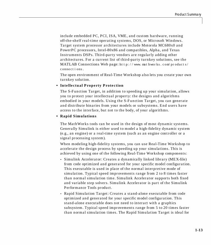
1-13
include embedded PC, PCI, ISA, VME, and custom hardware, runningoff-the-shelf real-time operating systems, DOS, or Microsoft Windows.Target system processor architectures include Motorola MC680x0 andPowerPC processors, Intel-80x86 and compatibles, Alpha, and TexasInstruments DSPs. Third-party vendors are regularly adding otherarchitectures. For a current list of third-party turnkey solutions, see theMATLAB Connections Web page: http://www.mathworks.com/products/connections.
The open environment of Real-Time Workshop also lets you create your ownturnkey solution.
• Intellectual Property Protection
The S-Function Target, in addition to speeding up your simulation, allowsyou to protect your intellectual property: the designs and algorithmsembodied in your models. Using the S-Function Target, you can generateand distribute binaries from your models or subsystems. End users haveaccess to the interface, but not to the body, of your algorithms.
• Rapid Simulations
The MathWorks tools can be used in the design of most dynamic systems.Generally Simulink is either used to model a high-fidelity dynamic system(e.g., an engine) or a real-time system (such as an engine controller or asignal processing system).
When modeling high-fidelity systems, you can use Real-Time Workshop toaccelerate the design process by speeding up your simulations. This isachieved by using one of the following Real-Time Workshop components:
- Simulink Accelerator: Creates a dynamically linked library (MEX-file)from code optimized and generated for your specific model configuration.This executable is used in place of the normal interpretive mode ofsimulation. Typical speed improvements range from 2 to 8 times fasterthan normal simulation time. Simulink Accelerator supports both fixedand variable step solvers. Simulink Accelerator is part of the SimulinkPerformance Tools product.
- Rapid Simulation Target: Creates a stand-alone executable from codeoptimized and generated for your specific model configuration. Thisstand-alone executable does not need to interact with a graphicssubsystem. Typical speed improvements range from 5 to 20 times fasterthan normal simulation times. The Rapid Simulation Target is ideal for
1 Introduction to the Real-Time Workshop
1-14
repetitive (batch) simulations where you are adjusting model parametersor coefficients. Rapid Simulation Target supports only fixed-step solvers.
- S-Function Target: This target, like Simulink Accelerator, creates adynamically linked library (MEX-file) from a model. You can incorporatethis component into another model using the Simulink S-function block.
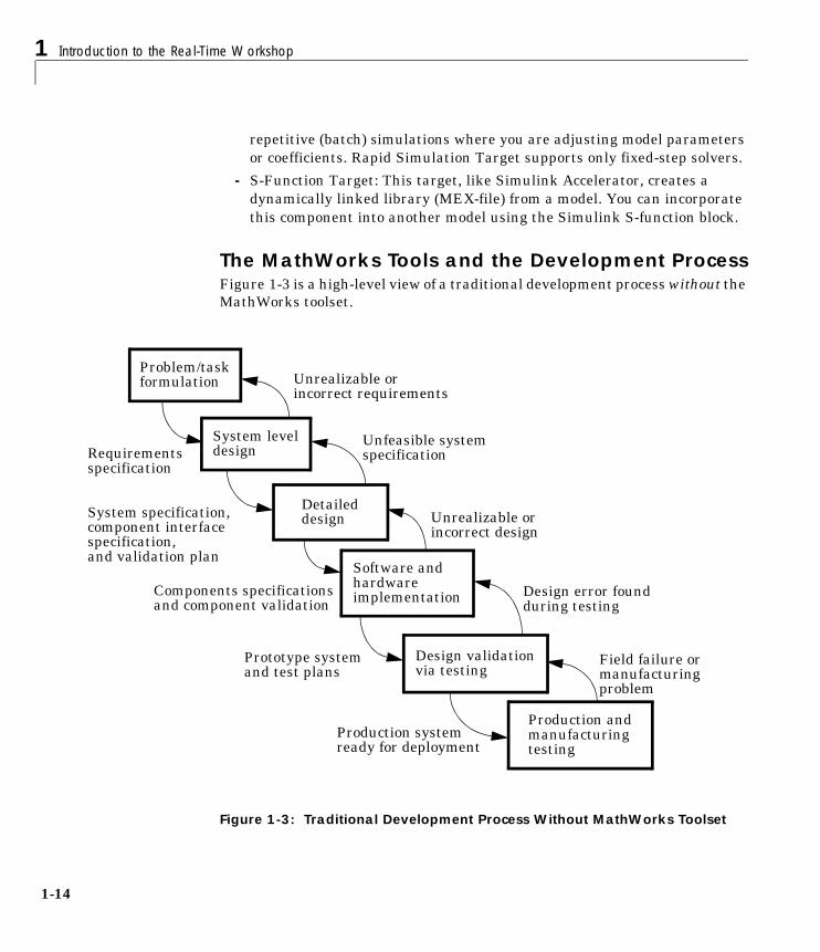
The MathWorks Tools and the Development ProcessFigure 1-3 is a high-level view of a traditional development process without theMathWorks toolset.
Figure 1-3: Traditional Development Process Without MathWorks Toolset
Problem/taskformulation
System leveldesignRequirements
specification
System specification,component interface
Components specificationsand component validation
specification,and validation plan
Detaileddesign
Software andhardwareimplementation
Design validationvia testing
Production andmanufacturingtesting
Prototype systemand test plans
Design error foundduring testing
Production systemready for deployment
Field failure ormanufacturing
Unrealizable orincorrect design
Unrealizable orincorrect requirements
problem
Unfeasible systemspecification
Product Summary
1-15
In Figure 1-3, each block represents a work phase. Documents are used tocoordinate the different work phases. In this environment, it is easy to go backone work phase, but hard to go back multiple work phases. In thisenvironment, design engineers (such as control system engineers or signalprocessing engineers) are not usually involved in the prototyping phase untilmany months after they have specified the design. This can result in poor timeto market and inferior quality.
In this environment, different tools are used in each phase. Designs arecommunicated via paper. This enforces a serial, rather than an iterative,development process. Developers must re-enter the result of the previousphase before they can begin work on a new phase. This leads tomiscommunication and errors, resulting in lost work hours. Errors found inlater phases are very expensive and time consuming to correct. Correctionoften involves going back several phases. This is difficult because of the poorcommunication between the phases.
The MathWorks does not suggest or impose a development process. TheMathWorks toolset can be used to complement any development process. In theabove process, use of our tools in each phase can help eliminate paper work.
Our toolset also lends itself well to the spiral design process shown inFigure 1-4.

1 Introduction to the Real-Time Workshop
1-16
Figure 1-4: Spiral Design Process
Using the MathWorks toolset, your model represents your understanding ofyour system. This understanding is passed from phase to phase in the model,reducing the need to go back to a previous phase. In the event that rework isnecessary in a previous phase, it is easier to transition back one or morephases, because the same model and tools are used in all phases.
A spiral design process iterates quickly between phases, enabling engineers towork on innovative features. The only way to do this cost effectively is to usetools that make it easy to move from one phase to another. For example, in amatter of minutes a control system engineer or a signal processing engineercan validate an algorithm on a real-world rapid prototyping system. The spiralprocess lends itself naturally to parallelism in the overall development process.You can provide early working models to validation and production groups,
DoneProblem/task
formulation
Software and
hardware
implementation
Production andmanufacturingtesting
StartS
ystemleveldesign
Detailed design
Design
validationvia
testing
Product Summary
1-17
involving them in your system development process from the start. This helpscompress the overall development cycle while increasing quality.
Another advantage of the MathWorks toolset is that it enables people to workon tasks that they are good at and enjoy doing. For example, control systemengineers specialize in design control laws, while embedded system engineersenjoy pulling together a system consisting of hardware and low-level software.It is possible to have very talented people perform different roles, but it is notefficient. Embedded system engineers, for example, are rewarded by specifyingand building the hardware and creating low-level software such as devicedrivers, or real-time operating systems. They do not find data entry operations,such as the manual conversion of a set of equations to efficient code, to berewarding. This is where the MathWorks toolset shines. The equations arerepresented as models and Real-Time Workshop converts them to highlyefficient code ready for deployment.

1 Introduction to the Real-Time Workshop
1-18
Role of the MathWorks Tools in Your Development ProcessThe following figure outlines where the MathWorks toolset, includingReal-Time Workshop, helps you in your development process.
Early in the design phase, you will start with MATLAB and Simulink to helpyou formulate your problems and create your initial design. Real-TimeWorkshop helps with this process by enabling high-speed simulations viaSimulink Accelerator (also part of Simulink Performance Tools), and theS-function Target for componentization and model speed-up.
After you have a functional model, you may need to tune your model’scoefficients. This can be done quickly using Real-Time Workshop’s Rapid
Simulink,
Interactive modeling and simulation
Stateflow, and Blocksetsand
Toolboxes
Customer definedmonitoring and
parameter tuning
High speed simulationAccelerator,
S-Function Targets
Interactive design
MATLAB
Rapid SimulationTarget
Batch design validation
Rapid Prototyping
Targets (real-time)
System development testing
Embedded
Code
Modules
Software unit testing
Embedded Codein Custom Target
Software integration
System testing and tuning
Embedded Codein Custom Target
Deployed system
Embedded Codein Custom Target
DesignCycle
Product Summary
1-19
Simulation Target for Monte-Carlo type simulations (varying coefficients overmany simulations).
After you’ve tuned your model, you can move into system development testingby exercising your model on a rapid prototyping system such as Real-TimeWindows Target or xPC Target. With a rapid prototyping target, you connectyour model to your physical system. This lets you locate design flaws ormodeling errors quickly.
After your prototype system is created, you can use Real-Time WorkshopEmbedded Coder to create embeddable code for deployment on your customtarget. The signal monitoring and parameter tuning capabilities enable you toeasily integrate the embedded code into a production environment equippedwith debugging and upgrade capabilities.
Code FormatsThe Real-Time Workshop code generator transforms your model to HLL code.Real-Time Workshop supports a variety of code formats designed for differentexecution environments, or targets.
In the traditional embedded system development process, an engineer developsan algorithm (or equations) to be implemented in an embedded system. Thesealgorithms are manually converted to a computer language such as C or Ada.This translation process, usually done by an embedded system engineer, ismuch like data entry.
Using Simulink to specify the algorithm (or equations), and Real-TimeWorkshop to generate corresponding code, engineers can bypass thisredundant translation step. This enables embedded system engineers to focuson the key issues involved in creating an embedded system: the hardwareconfiguration, device drivers, supervisory logic, and supporting logic for themodel equations. Simulink itself is the programming language that expressesthe algorithmic portion of the system.
1 Introduction to the Real-Time Workshop
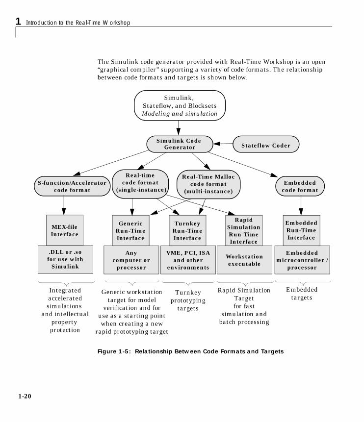
1-20
The Simulink code generator provided with Real-Time Workshop is an open“graphical compiler” supporting a variety of code formats. The relationshipbetween code formats and targets is shown below.
Figure 1-5: Relationship Between Code Formats and Targets
Real-timecode format
(single-instance)
Simulink,
Modeling and simulationStateflow, and Blocksets
Simulink CodeStateflow Coder
Embeddedcode format
S-function/Acceleratorcode format
Real-Time Malloccode format
EmbeddedRun-TimeInterface
Embeddedmicrocontroller /
processor
GenericRun-TimeInterface
Anycomputer or
processor
TurnkeyRun-TimeInterface
VME, PCI, ISAand other
environments
Embeddedtargets
Turnkeyprototyping
targets
Generic workstationtarget for model
verification and foruse as a starting pointwhen creating a new
rapid prototyping target
RapidSimulationRun-Time
Workstation
Interface
executable
Rapid SimulationTargetfor fast
simulation andbatch processing
MEX-fileInterface
.DLL or .sofor use with
Simulink
Integratedacceleratedsimulations
and intellectualpropertyprotection
Generator
(multi-instance)
Product Summary
1-21
S-Function/Accelerator Code FormatThis code format, used by the S-Function Target and Simulink Accelerator,generates code that conforms to Simulink C MEX S-function API.
Real-Time Code FormatThe real-time code format is ideally suited for rapid prototyping. This codeformat (C only) supports increased monitoring and tuning capabilities,enabling easy connection with external mode. Real-time code format supportscontinuous-time models, discrete-time single- or multirate models, and hybridcontinuous-time and discrete-time models. Real-time code format supportsboth inlined and noninlined S-functions. Memory allocation is declaredstatically at compile time.
Real-Time Malloc Code FormatThe real-time malloc code format is similar to the real-time code format. Theprimary difference is that the real-time malloc code format declares memorydynamically. This supports multiple instances of the same model, with eachinstance including a unique data set. Multiple models can be combined into oneexecutable without name clashing. Multiple instances of a given model can alsobe created in one executable.
Embedded Code FormatThe embedded code format is designed for embedded targets. The generatedcode is optimized for speed, memory usage, and simplicity. Generally, thisformat is used in deeply embedded or deployed applications. There are nodynamic memory allocation calls; all persistent memory is statically allocated.Real-Time Workshop can generate either C or Ada code in the embedded codeformat. Note Ada code requires Real-Time Workshop Ada Coder, an add-onproduct.
The embedded code format provides a simplified calling interface and reducedmemory usage. This format manages model and timing data in a compactreal-time object structure. This contrasts with the other code formats, whichuse a significantly larger, model-independent Simulink data structure(SimStruct) to manage the generated code.
The embedded code format improves readability of the generated code, reducescode size, and speeds up execution. The embedded code format supports alldiscrete-time single- or multirate models.
1 Introduction to the Real-Time Workshop
1-22
Because of its optimized and specialized data structures, the embedded codeformat supports only inlined S-functions.
Target EnvironmentsThe Real-Time Workshop supports many target environments. These includeready-to-run configurations and third-party targets. You can also develop yourown custom target.
This section begins with a list of available target configurations. Following thelist, we summarize the characteristics of each target.
Available Target Configurations
Target Configurations Bundled with Real-Time Workshop. The MathWorks suppliesthe following target configurations with Real-Time Workshop:
• DOS (4GW) Target (example only)
• Generic Real-Time (GRT) Target
• LE/O (Lynx Embedded OSEK) Real-Time Target (example only)
• Rapid Simulation Target
• Tornado (VxWorks) Real-Time Target
Target Configurations Bundled with Real-Time Workshop Ada Coder. The MathWorkssupplies the following target configurations with Real-Time Workshop AdaCoder (a separate product from the Real-Time Workshop):
• Ada Real-Time Multitasking Target
• Ada Simulation Target
Target Configurations Bundled with Real-Time Workshop Embedded Coder. TheMathWorks supplies the following target configuration with Real-TimeWorkshop Embedded Coder (a separate product from the Real-TimeWorkshop):
• Real-Time Workshop Embedded Coder Target
Turnkey Rapid Prototyping Target Products. These self-contained solutions ( separateproducts from the Real-Time Workshop) include:
• Real-Time Windows Target
Product Summary
1-23
• xPC Target
DSP Target Products. See Texas Instruments DSP Developer's Kit User’s Guide forinformation on these targets:
• Texas Instruments Code Composer Studio Target
• Texas Instruments EVM67x Target
Third-Party Targets. Numerous software vendors have developed customizedtargets for the Real-Time Workshop. For an up-to-date listing of third-partytargets, visit the MATLAB Connections Web page at http://www.mathworks.com/products/connections
View Third-Party Solutions by Product Type, and then select RTW Target.
Custom Targets. Typically, to target custom hardware, you must write a harness(main) program for your target system to execute the generated code, and I/Odevice drivers to communicate with your hardware. You must also create asystem target file and a template makefile.
The Real-Time Workshop supplies generic harness programs as starting pointsfor custom targeting. Chapter 17, “Targeting Real-Time Systems” provides theinformation you will need to develop a custom target.
Rapid Simulation TargetRapid Simulation Target (RSIM) consists of a set of target files fornon-real-time execution on your host computer. RSIM enables you to use theReal-Time Workshop to generate fast, stand-alone simulations. RSIM allowsbatch parameter tuning and downloading of new simulation data (signals)from a standard MATLAB MAT-file without the need to recompile the model.
The speed of the generated code also makes RSIM ideal for Monte Carlosimulations. The RSIM target enables the generated code to read and writedata from or to standard MATLAB MAT-files. RSIM reads new signals andparameters from MAT-files at the start of simulation.
RSIM enables you to run stand-alone, fixed-step simulations on your hostcomputer or on additional computers. If you need to run 100 large simulations,you can generate the RSIM model code, compile it, and run the executables on10 identical computers. The RSIM target allows you to change the modelparameters and the signal data, achieving significant speed improvements byusing a compiled simulation.
1 Introduction to the Real-Time Workshop
1-24
S-Function and Accelerator TargetsS-Function Target provides the ability to transform a model into a SimulinkS-function component. Such a component can then be used in a larger model.This allows you to speed up simulations and/or reuse code. You can includemultiple instances of the same S-function in the same model, with eachinstance maintaining independent data structures. You can also shareS-function components without exposing the details of the a proprietary sourcemodel.
The Accelerator Target is similar to the S-Function Target in that anS-function is created for a model. The Accelerator Target differs from theS-Function Target in that the generated S-function operates in thebackground. It provides for faster simulations while preserving all existingsimulation capabilities (parameter change, signal visualization, full S-functionsupport, etc.).
Turnkey Rapid Prototyping TargetsReal-Time Windows Target and xPC Target are add-on products to Real-TimeWorkshop. Both of these targets turn an Intel 80x86/Pentium or compatible PCinto a real-time system. Both support a large selection of off-the-shelf I/O cards(both ISA and PCI).
With turnkey target systems, all you need to do is install the MathWorkssoftware and a compiler, and insert the I/O cards. You can then use a PC as areal-time system connected to external devices via the I/O cards.
Real-Time Windows Target. Real-Time Windows Target brings rapid prototypingand hardware-in-the-loop simulation to your desktop. It is the most portablesolution available today for rapid prototyping and hardware-in-the-loopsimulation when used on a laptop outfitted with a PCMCIA I/O card.Real-Time Windows Target is ideal since a second PC or other real-timehardware is often unnecessary, impractical or cumbersome.
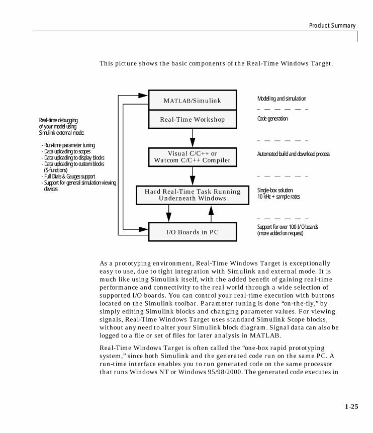
Product Summary
1-25
This picture shows the basic components of the Real-Time Windows Target.
As a prototyping environment, Real-Time Windows Target is exceptionallyeasy to use, due to tight integration with Simulink and external mode. It ismuch like using Simulink itself, with the added benefit of gaining real-timeperformance and connectivity to the real world through a wide selection ofsupported I/O boards. You can control your real-time execution with buttonslocated on the Simulink toolbar. Parameter tuning is done “on-the-fly,” bysimply editing Simulink blocks and changing parameter values. For viewingsignals, Real-Time Windows Target uses standard Simulink Scope blocks,without any need to alter your Simulink block diagram. Signal data can also belogged to a file or set of files for later analysis in MATLAB.
Real-Time Windows Target is often called the “one-box rapid prototypingsystem,” since both Simulink and the generated code run on the same PC. Arun-time interface enables you to run generated code on the same processorthat runs Windows NT or Windows 95/98/2000. The generated code executes in
MATLAB/Simulink
Real-Time Workshop
Visual C/C++ orWatcom C/C++ Compiler
Hard Real-Time Task RunningUnderneath Windows
I/O Boards in PC
Modeling and simulation
Code generation
Automated build and download process
Single-box solution10 kHz + sample rates
Support for over 100 I/O boards(more added on request)
Real-time debuggingof your model usingSimulink external mode:
- Run-time parameter tuning- Data uploading to scopes- Data uploading to display blocks- Data uploading to custom blocks
(S-functions)- Full Dials & Gauges support- Support for general simulation viewing
devices

1 Introduction to the Real-Time Workshop
1-26
hard real-time, allowing Windows to execute when there are free CPU cycles.Real-Time Windows Target supports over 100 I/O boards, including ISA, PCI,CompactPCI, and PCMCIA. Sample rates in excess of 10 to 20 kHz can beachieved on Pentium PCs.
In universities, Real-Time Windows Target provides a cost effective solutionsince only a single computer is required. In commercial applications,Real-Time Windows Target is often used at an engineer’s desk prior to takinga project to an expensive dedicated real-time testing environment. Itsportability is unrivaled, allowing you to use your laptop as a real-time test bedfor applications in the field.
Figure 1-6 illustrates the use of Real-Time Windows Target in a model usingmagnetic levitation to suspend a metal ball in midair. The system is controlledby the model shown in Figure 1-7.
Figure 1-6: Magnetic Levitation System
Electromagnet
Proximity sensor
Metallic ball
PMCIA I/O
Sensor and actuator connector cable
Real-TimeWorkshop
Simulink &
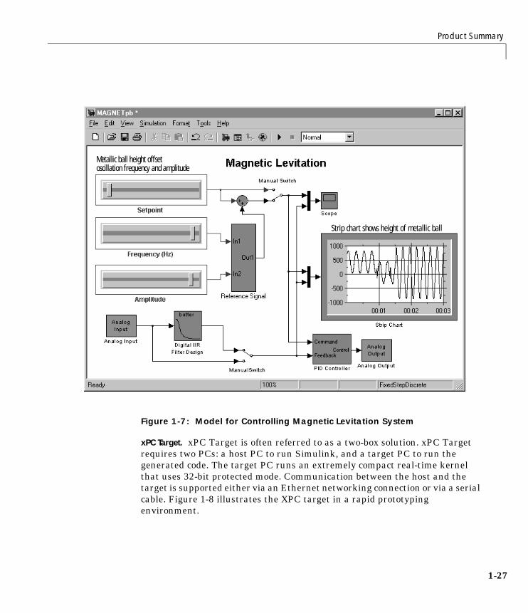
Product Summary
1-27
Figure 1-7: Model for Controlling Magnetic Levitation System
xPC Target. xPC Target is often referred to as a two-box solution. xPC Targetrequires two PCs: a host PC to run Simulink, and a target PC to run thegenerated code. The target PC runs an extremely compact real-time kernelthat uses 32-bit protected mode. Communication between the host and thetarget is supported either via an Ethernet networking connection or via a serialcable. Figure 1-8 illustrates the XPC target in a rapid prototypingenvironment.
Strip chart shows height of metallic ball
Metallic ball height offsetoscillation frequency and amplitude
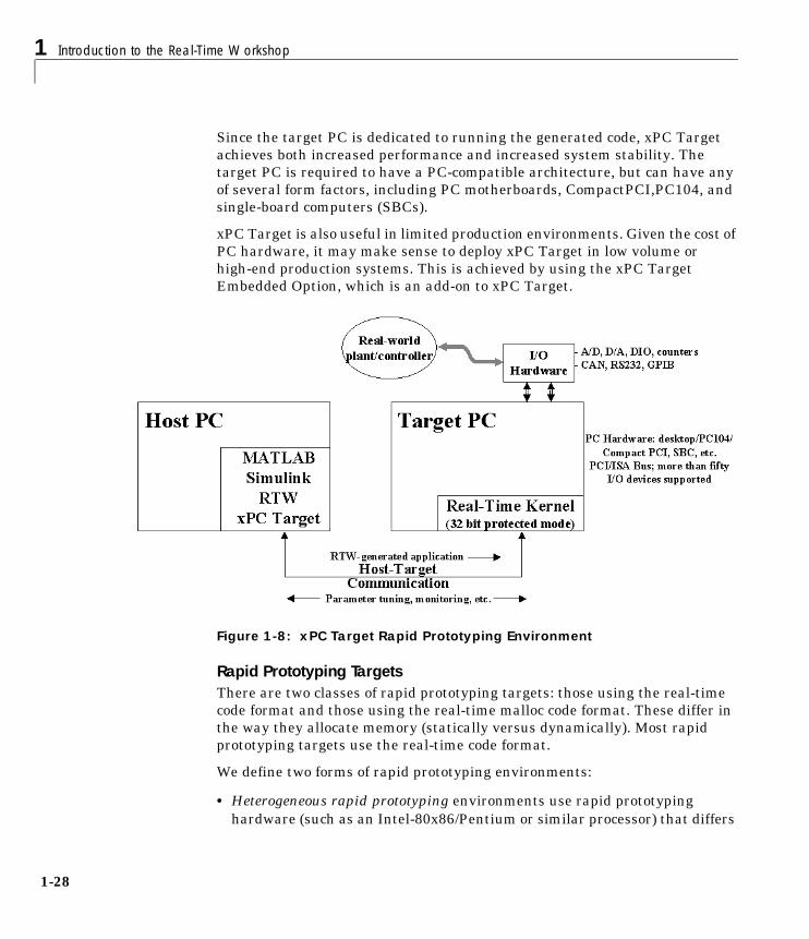
1 Introduction to the Real-Time Workshop
1-28
Since the target PC is dedicated to running the generated code, xPC Targetachieves both increased performance and increased system stability. Thetarget PC is required to have a PC-compatible architecture, but can have anyof several form factors, including PC motherboards, CompactPCI,PC104, andsingle-board computers (SBCs).
xPC Target is also useful in limited production environments. Given the cost ofPC hardware, it may make sense to deploy xPC Target in low volume orhigh-end production systems. This is achieved by using the xPC TargetEmbedded Option, which is an add-on to xPC Target.
Figure 1-8: xPC Target Rapid Prototyping Environment
Rapid Prototyping TargetsThere are two classes of rapid prototyping targets: those using the real-timecode format and those using the real-time malloc code format. These differ inthe way they allocate memory (statically versus dynamically). Most rapidprototyping targets use the real-time code format.
We define two forms of rapid prototyping environments:
• Heterogeneous rapid prototyping environments use rapid prototypinghardware (such as an Intel-80x86/Pentium or similar processor) that differs
Product Summary
1-29
from the final production hardware. For example, an Intel-80x86/Pentium orsimilar processor might be used during rapid prototyping of a system that iseventually deployed onto a fixed-point Motorola microcontroller.
• Homogeneous rapid prototyping environments are characterized by the useof similar hardware for the rapid prototyping system and the finalproduction system. The main difference is that the rapid prototyping systemhas extra memory and/or interfacing hardware to support increaseddebugging capabilities, such as communication with external mode.
Homogeneous rapid prototyping environments eliminate uncertainty becausethe rapid prototyping environment is closer to the final production system.However, a turnkey system for your specific hardware may not exist. In thiscase, you must weigh the advantages and disadvantages of using one of theexisting turnkey systems for heterogeneous rapid prototyping, versus creatinga homogeneous rapid prototyping environment.
Several rapid prototyping targets are bundled with Real-Time Workshop.
Generic Real-Time (GRT) Target. This target uses the real-time code format andsupports external mode communication. It is designed to be used as a startingpoint when creating a custom rapid prototyping target, or for validating thegenerated code on your workstation.
Generic Real-Time Malloc (GRTM) Target. This target is similar to the GRT targetbut it uses the real-time malloc code format. This format uses the C malloc andfree routines to manage all data. With this code format, you can have multipleinstances of your model and/or multiple models in one executable.
Tornado Target. The Tornado target uses the real-time or real-time malloc codeformat. A set of run-time interface files are provided to execute your models onthe Wind River System’s real-time operating system, VxWorks. The Tornadotarget supports singletasking, multitasking, and hybrid continuous anddiscrete-time models.
The Tornado run-time interface and device driver files can also be used as astarting point when targeting other real-time operating system environments.The run-time interface provides full support for external mode, enabling you totake full advantage of the debugging capabilities for parameter tuning anddata monitoring via graphical devices.
1 Introduction to the Real-Time Workshop
1-30
DOS Target. The DOS target (provided as an example only) uses the real-timecode format to turn a PC running the DOS operating system into a real-timesystem. This target includes a set of run-time interface files for executing thegenerated code. This run-time interface installs interrupt service routines toexecute the generated code and handle other interrupts. While the DOS targetis running, the user does not have access to the DOS operating system. Sampledevice drivers are provided.
The MathWorks recommends that you use Real-Time Windows Target or xPCTarget as alternatives to the DOS Target. The DOS target is provided only asan example and its support will be discontinued in the future.
OSEK Targets. The OSEK target (provided as an example only) lets you use theautomotive standard open real-time operating system. The run-time interfaceand OSEK configuration files that are included with this target make it easyto port applications to a wide range of OSEK environments.
Embedded TargetsThe embedded real-time target is the main component of the Real-TimeWorkshop Embedded Coder. It consists of a set of run-time interface files thatdrive code, generated in the embedded code format, on your workstation. Thistarget is ideal for memory-constrained embedded applications. Real-TimeWorkshop supports generation of embedded code in both C and Ada.
In its default configuration, the embedded real-time target is designed for useas a starting point for targeting custom embedded applications, and as a meansby which you can validate the generated code. To create a custom embeddedtarget, you start with the embedded real-time target run-time interface filesand edit them as needed for your application.
In the terminology of Real-Time Workshop, an embedded target is a deeplyembedded system. Note that it is possible to use a rapid prototyping target inan embedded (production) environment. This may make more sense in yourapplication.
Code Generation OptimizationsThe Simulink code generator included with Real-Time Workshop is packedwith optimizations to help create fast and minimal size code. The optimizationsare classified either as cross-block optimizations, or block specificoptimizations. Cross-block optimizations apply to groups of blocks or the
Product Summary
1-31
general structure of a model. Block specific optimizations are handled locallyby the object generating code for a given block. Listing each block specificoptimization here is not practical; suffice it to say that the Target LanguageCompiler technology generates very tight and fast code for each block in yourmodel.
The following sections discuss some of the cross-block optimizations.
Multirate SupportOne of the more powerful features of Simulink is its implicit support formultirate systems. The ability to run different parts of a model at differentrates guarantees optimal use of the target processor. In addition, Simulinkenforces correctness by requiring that you create your model in a manner thatguarantees deterministic execution.
Inlining S-Function Blocks for Optimal CodeThe ability to add blocks to Simulink via S-functions is enhanced by the TargetLanguage Compiler. You can create blocks that embed the minimal amount ofinstructions into the generated code. For example, if you create a device driverusing an S-function, you can have the generated code produce one line for thedevice read, as in the following code fragment.
mdlOutputs(void){
.
.rtB.deviceout = READHW(); /* Macro to read hw device using . assembly code */.
}
Note that the generic S-function API is suitable for any basic block-typeoperation.
Loop Rolling ThresholdThe code generated for blocks can contain for loops, or the loop iterations canbe “flattened out” into inline statements. For example, the general gain blockequation is
for (i = 0; i < N; i++) {y[i] = k[i] * u[i];
}
1 Introduction to the Real-Time Workshop
1-32
If N is less than a specified roll threshold, Real-Time Workshop expands out thefor loop, otherwise Real-Time Workshop retains the for loop.
Tightly Coupled Optimal Stateflow InterfaceThe generated code for models that combine Simulink blocks and Stateflowcharts is tightly integrated and very efficient.
Stateflow OptimizationsThe Stateflow Coder contains a large number of optimizations that producehighly readable and very efficient generated code.
Inlining of SystemsIn Simulink, a system starting at a nonvirtual subsystem boundary (e.g. anenabled, triggered, enabled and triggered, function-call, or atomic subsystem)can be inlined by selecting the RTW inline subsystem option from thesubsystem block properties dialog. The default action is to inline thesubsystem, unless it is a function-call subsystem with multiple callers.
Block I/O ReuseConsider a model with a D/A converter feeding a gain block (for scaling), thenfeeding a transfer function block, then feeding a A/D block. If all signals referto the same memory location, then less memory will be used. This is referredto as block I/O reuse. It is a powerful optimization technique for re-usingmemory locations. It reduces the number of global variables improving theexecuting speed (faster execution) and reducing the size of the generated code.
Declaration of Block I/O Variables in Local ScopeIf input/output signal variables are not used across function scope, then theycan be placed in local scope. This optimization technique reduces code size andimproves the execution speed (faster execution).
Inlining of ParametersIf you select the Inline parameters option, the numeric values of blockparameters that represent coefficients are embedded in the generated code. IfInline parameters is off, block parameters that represent coefficients can bechanged while the model is executing.

Product Summary
1-33
Note that it is still possible to “tune” key parameters by using the Workspaceparameter attributes dialog.
Inlining of Invariant SignalsAn invariant signal is a block output signal that does not change duringSimulink simulation. For example, the output of a sum block that is fed by twoconstants cannot change. When Inline invariant signals is specified, a singlenumeric value is placed in the generated code to represent the output value ofthe sum block. The Inline invariant signals option is available when theInline parameters option is on.
Parameter PoolingThe Parameter pooling option is available when Inline parameters isselected. If Real-Time Workshop detects identical usage of parameters (e.g. twolookup tables with same tables), it will pool these parameters together, therebyreducing code size.
Block Reduction OptimizationsReal-Time Workshop can detect block patterns (e.g. an accumulatorrepresented by a constant, sum and a delay block) and reduce these patterns toa single operation, resulting in very efficient generated code.
Creation of Contiguous Signals to Speed Block ComputationsSome block algorithms (for example a matrix multiply) can be implementedmore efficiently if the signals entering the blocks are contiguous.Noncontiguous signals occur because of the handling of virtual blocks. Forexample, the output of a Mux block is noncontiguous. When this class of blockrequires a contiguous signal, Simulink will insert (if needed) a copy blockoperator to make the signal contiguous. This results in better code efficiency.
Support for Noncontiguous Signals by BlocksNoncontiguous signals occur because of the block virtualization capabilities ofSimulink. For example, the output of a Mux block is generally a noncontiguoussignal (i.e., the output signal consists of signals from multiple sources). Generalblocks in Simulink support this behavior by generating very efficient code tohandle each different signal source in a noncontiguous signal.
1 Introduction to the Real-Time Workshop
1-34
Data Type SupportSimulink models support a wide range of data types. You can use doubleprecision values to represent real-world values and then when needed useintegers or Booleans for discrete valued signals. You can also use fixed-point(integer scaling) capabilities to target models for fixed-point embeddedprocessors. The wide selection of data types in Simulink models enables you torealize your models efficiently.
Frame SupportIn signal processing, a frame of data represents time sampled sequences of aninput. Many devices have support in hardware for collecting frames of data.With Simulink and the DSP Blockset, you can use frames and perform framebased operations on the data. Frames are a very efficient way of handling highfrequency signal processing applications.
Matrix SupportMost blocks in Simulink support the use of matrices. This enables you to createmodels that represent high levels of abstractions and produce very efficientgenerated code.
Virtualization of BlocksNearly half of the blocks in a typical model are connection type blocks (e.g.Virtual Subsystem, Inport, Outport, Goto, From, Data Store Memory, Selector,Bus Selector, Mux, Demux, Ground, and Terminator). These blocks areprovided to enable you to create complex models with your desired levels ofabstraction. Simulink treats these blocks as virtual, meaning that they imposeno overhead during simulation or in the generated code.
Open and Extensible Modeling EnvironmentThe Simulink / Real-Time Workshop environment is extensible in severalways.
Custom Code SupportS-functions are dynamically linked objects (.DLL or .so) that bind withSimulink to extend the modeling environment. By developing S-functions, youcan add custom block algorithms to Simulink. Such S-functions providesupporting logic for the model. S-functions are flexible, allowing you to

Product Summary
1-35
implement complex algorithmic equations or basic low-level device drivers. TheReal-Time Workshop support for S-functions includes the ability to inlineS-function code directly into the generated code. Inlining, supported by theTarget Language Compiler, can significantly reduce memory usage and callingoverhead.
Support for Supervisory CodeThe generated code implements an algorithm that corresponds exactly to thealgorithm defined in your model. With the embedded code format, you can callthe generated model code as a procedure. This enables you to incorporate thegenerated code into larger systems that decide when to execute the generatedcode. Conceptually, you can think of the generated code as set of equations,wrapped in a function called by your supervisory code. This facilitatesintegration of model code into large existing systems, or into environments thatconsist of more than signal-flow processing (Simulink) and state machines(Stateflow).
Monitoring and Parameter Tuning APIsExternal mode provides a communication channel for interfacing thegenerated code running on your target with Simulink. External mode lets youuse Simulink as a debugging front end for an executing model. Typically, theexternal mode configuration works in conjunction with either the real-timecode format or the real-time malloc code format.
The Real-Time Workshop provides other mechanisms for making modelsignals and block parameters visible to your own monitoring and tuninginterfaces. These mechanisms, suitable for use on all code formats, include:
• The Model Parameter Configuration dialog enables you to declare how toallocate memory for variables that are used in your model. For example, if aGain block contains the variable k, you can declare k as an external variable,a pointer to an external variable, a global variable, or let the Real-TimeWorkshop decide where and how to declare the variable.
The Model Parameter Configuration feature enables you to specify blockparameters as tunable or global. This gives your supervisory code completeaccess to any block parameter variables that you may need to alter whileyour model is executing. You can also use this feature to interfaceparameters to specific constant read-only memory locations.
1 Introduction to the Real-Time Workshop
1-36
• You can mark signals in your model as test points. Declaring a test pointindicates that you may want to see the signal’s value while the model isexecuting. After marking a signal as a test point, you specify how thememory for the signal is to be allocated. This gives your supervisory codecomplete read-only access to signals in your model, so that you can monitorthe internal workings of your model.
• C and Target Language Compiler APIs provide another form of access to thesignals and parameters in your model. The Target Language Compiler APIis a means to access the internal signals and parameters during codegeneration. With this information, you can generate monitoring/tuning codethat is optimized specifically for your model or target.
Interrupt SupportInterrupt blocks enable you to create models that handle synchronous andasynchronous events, including interrupt service routines (ISRs),hardware-generated interrupts, and asynchronous read and write operations.The blocks provided work with the Tornado target. You can use these blocks astemplates when creating new interrupt blocks for your target environment.Interrupt blocks include:
• Asynchronous Interrupt block
• Task Synchronization block
• Asynchronous Buffer block (read)
• Asynchronous Buffer block (write)
• Asynchronous Rate Transition block
Custom Code LibraryThe Custom Code library contains a set of blocks that allow you to easily inserttarget-specific code into your model without the need of an inlined S-function.Code can be placed strategically throughout the model.
Getting Started: Basic Concepts and Tutorials
1-37
Getting Started: Basic Concepts and TutorialsThis section is designed to help you to obtain hands-on experience with theReal-Time Workshop in short order. There are two parts, which we recommendyou read in order:
1 “Basic Real-Time Workshop Concepts” on page 1-37 introduces concepts andterminology you should know before working with the Real Time Workshop.
2 “Quick Start Tutorials” on page 1-40 provides several hands-on exercisesthat demonstrate the Real-Time Workshop user interface, code generationand build process, and other essential features.
Basic Real-Time Workshop Concepts
Target and HostA target is an environment — hardware or operating system — on which yourgenerated code will run. The process of specifying this environment is calledtargeting.
The process of generating target-specific code is controlled by a system targetfile, a template makefile, and a make command. To select a desired target, youcan specify these items individually, or you can choose from a wide variety ofready-to-run configurations.
The host is the system you use to run MATLAB, Simulink, and the Real-TimeWorkshop. Using the build tools on the host, you create code and an executablethat runs on your target system.
Available Target ConfigurationsThe Real-Time Workshop supports many target environments. These includeready-to-run configurations and third-party targets. You can also develop yourown custom target.
For a complete list of bundled targets, with their associated system target filesand template makefiles, see “The System Target File Browser” on page 3-34.
Code FormatsA code format specifies a framework for code generation suited for specificapplications.
1 Introduction to the Real-Time Workshop
1-38
When you choose a target configuration, you implicitly choose a code format. Ifyou use the Real-Time Workshop Embedded Coder, for example, the codegenerated will be in embedded C format. The embedded C code format is acompact format designed for production code generation. Its small code size,memory usage, and simple call structure make it optimal for embeddedapplications.
Many other targets, such as the generic real-time (GRT) target, use thereal-time code format. This format, less compact but more flexible, is optimalfor rapid prototyping applications.
For a complete discussion of available code formats, see Chapter 4, “GeneratedCode Formats.”
The Generic Real-Time TargetThe Real-Time Workshop provides a generic real-time development target. Thegeneric real-time (GRT) target provides an environment for simulatingfixed-step models in single or multitasking mode. A program generated withthe GRT target runs your model, in simulated time, as a stand-alone programon your workstation.
The GRT target allows you to perform code validation by logging systemoutputs, states, and simulation time to a data file. The data file can then beloaded into the MATLAB workspace for analysis or comparison with the outputof the original model.
The GRT target also provides a starting point for targeting custom hardware.You can modify the GRT harness program, grt_main.c, to execute codegenerated from your model at interrupt level under control of a real-time clock.
Target Language Compiler FilesThe Real-Time Workshop uses Target Language Compiler files (or TLC files) totranslate your Simulink model into code. The Target Language Compiler usestwo types of TLC files during the code generation and build process. The systemtarget file, which describes how to generate code for a chosen target, is the entrypoint for the TLC program that creates the executable. Block target files definehow the code looks for each of the Simulink blocks in your model.
System and block target files have the extension .tlc. By convention, a systemtarget file has a name corresponding to your target. For example, grt.tlc isthe system target file for the generic real-time (GRT) target.
Getting Started: Basic Concepts and Tutorials
1-39
Template MakefilesThe Real-Time Workshop uses template makefiles to build an executable fromthe generated code.
The Real-Time Workshop build process creates a makefile from the templatemakefile. Each line from the template makefile is copied into the makefile;tokens encountered during this process are expanded into the makefile.
The name of the makefile created by the build process is model.mk. Themodel.mk file is passed to a make utility. The make utility compiles and linksan executable from a set of files.
By convention, a template makefile has an extension of .tmf and a namecorresponding to your target and compiler. For example, grt_vc.tmf is thetemplate makefile for building a generic real-time program under Visual C/C++.
The Build ProcessA high-level M-file command controls the Real-Time Workshop build process.The default command, used with most targets, is make_rtw.When you initiatea build, the Real-Time Workshop invokes make_rtw.The make_rtw command, inturn, invokes the Target Language Compiler and other utilities such as make.The build process consists of the following stages:
1 First, make_rtw compiles the block diagram and generates a modeldescription file, model.rtw.
2 Next, make_rtw invokes the Target Language Compiler to generatetarget-specific code, processing model.rtw as specified by the selectedsystem target file.
3 Next, make_rtw creates a makefile, model.mk, from the selected templatemakefile.
4 Finally, make is invoked. make compiles and links a program from thegenerated code, as instructed in the generated makefile.
“Automatic Program Building” in Chapter 2 gives an overview of the buildprocess. Chapter 3, “Code Generation and the Build Process” gives full detailson code generation and build options and parameters.
1 Introduction to the Real-Time Workshop
1-40
Model Parameters and Code GenerationThe simulation parameters of your model directly affect code generation andprogram building. For example, if your model is configured to stop executionafter 60 seconds, the program generated from your model will also run for 60seconds. The Real-Time Workshop also imposes certain requirements andrestrictions on the model from which code is generated.
Before you generate code and build an executable, you must verify that youhave set the model parameters correctly in the Simulation Parameters dialogbox. See “Simulation Parameters and Code Generation” in Chapter 3 for moreinformation.
Quick Start TutorialsThis section provides hands-on experience with the code generation, programbuilding, data logging, and code validation capabilities of the Real-TimeWorkshop.
“Tutorial 1: Building a Generic Real-Time Program” on page 1-42 shows how togenerate C code from a Simulink demonstration model and build an executableprogram.
“Tutorial 2: Data Logging” on page 1-49 explains how to modify thedemonstration program to save data in a MATLAB MAT-file, for plotting.
“Tutorial 3: Code Validation” on page 1-52, demonstrates how to validate thegenerated program by comparing its output to that of the original model.
“Tutorial 4: A First Look at Generated Code” on page 1-56 examines codegenerated from a very simple model, illustrating the effect of one of theReal-Time Workshop code generation options.
These tutorials assume basic familiarity with MATLAB and Simulink. Youshould also read “Getting Started: Basic Concepts and Tutorials” on page 1-37before proceeding.
The procedures for building, running, and testing your programs are almostidentical in UNIX and PC environments. The discussion notes differenceswhere applicable.
Make sure that a MATLAB compatible C compiler is installed on your systembefore proceeding with these tutorials. See the “Preface” for more informationon supported compilers and compiler installation.

Getting Started: Basic Concepts and Tutorials
1-41
The f14 Demonstration Model Tutorials 1-3 use a demonstration Simulink model, f14.mdl, from thematlabroot/toolbox/simulink/simdemos/aerospace directory. (By default,this directory is on your MATLAB path.) f14 is a model of a flight controller forthe longitudinal motion of a Grumman Aerospace F-14 aircraft.
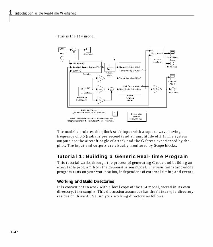
1 Introduction to the Real-Time Workshop
1-42
This is the f14 model.
The model simulates the pilot’s stick input with a square wave having afrequency of 0.5 (radians per second) and an amplitude of ± 1. The systemoutputs are the aircraft angle of attack and the G forces experienced by thepilot. The input and outputs are visually monitored by Scope blocks.
Tutorial 1: Building a Generic Real-Time ProgramThis tutorial walks through the process of generating C code and building anexecutable program from the demonstration model. The resultant stand-aloneprogram runs on your workstation, independent of external timing and events.
Working and Build DirectoriesIt is convenient to work with a local copy of the f14 model, stored in its owndirectory, f14example. This discussion assumes that the f14example directoryresides on drive d:. Set up your working directory as follows:

Getting Started: Basic Concepts and Tutorials
1-43
1 Create the directory from the MATLAB command line by typing
!mkdir d:\f14example (on PC)
or
!mkdir ~/f14example (on UNIX)
2 Make f14example your working directory.
cd d:/f14example
3 Open the f14 model.
f14
The model appears in the Simulink window.
4 From the File menu, choose Save As. Save a copy of the f14 modelas d:/f14example/f14rtw.mdl.
Be aware that during code generation, the Real-Time Workshop creates a builddirectory within your working directory. The build directory name ismodel_target_rtw, derived from the name of the source model and the chosentarget. The build directory stores generated source code and other files createdduring the build process. We examine the build directory and its contents at theend of this tutorial.
Setting Program ParametersTo generate code correctly from the f14rtw model, you must change some of thesimulation parameters. In particular, note that the Real-Time Workshoprequires the use of a fixed-step solver. To set parameters, use the SimulationParameters dialog box as follows:
1 From the Simulation menu, choose Simulation Parameters. TheSimulation Parameters dialog box opens.

1 Introduction to the Real-Time Workshop
1-44
2 Click the Solver tab and enter the following parameter values on the Solverpage.
Start Time: 0.0
Stop Time: 60
Solver options: set Type to Fixed-step. Select the ode5 (Dormand-Prince) solver algorithm.
Fixed step size: 0.05
Mode: Single Tasking
3 Click Apply. Then click OK to close the dialog box.
4 Save the model. Simulation parameters persist with the model, for use infuture sessions.
Figure 1-9 shows the Solver page with the correct parameter settings.
Figure 1-9: Solver Page of Simulation Parameters Dialog Box
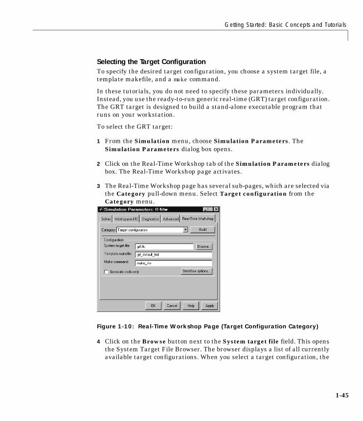
Getting Started: Basic Concepts and Tutorials
1-45
Selecting the Target ConfigurationTo specify the desired target configuration, you choose a system target file, atemplate makefile, and a make command.
In these tutorials, you do not need to specify these parameters individually.Instead, you use the ready-to-run generic real-time (GRT) target configuration.The GRT target is designed to build a stand-alone executable program thatruns on your workstation.
To select the GRT target:
1 From the Simulation menu, choose Simulation Parameters. TheSimulation Parameters dialog box opens.
2 Click on the Real-Time Workshop tab of the Simulation Parameters dialogbox. The Real-Time Workshop page activates.
3 The Real-Time Workshop page has several sub-pages, which are selected viathe Category pull-down menu. Select Target configuration from theCategory menu.
Figure 1-10: Real-Time Workshop Page (Target Configuration Category)
4 Click on the Browse button next to the System target file field. This opensthe System Target File Browser. The browser displays a list of all currentlyavailable target configurations. When you select a target configuration, the
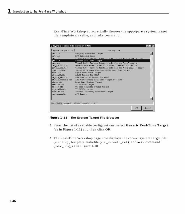
1 Introduction to the Real-Time Workshop
1-46
Real-Time Workshop automatically chooses the appropriate system targetfile, template makefile, and make command.
Figure 1-11: The System Target File Browser
5 From the list of available configurations, select Generic Real-Time Target(as in Figure 1-11) and then click OK.
6 The Real-Time Workshop page now displays the correct system target file(grt.tlc), template makefile (grt_default_tmf), and make command(make_rtw), as in Figure 1-10.

Getting Started: Basic Concepts and Tutorials
1-47
7 Select General code generation options from the Category menu. Theoptions displayed here are common to all target configurations. Check tomake sure that all options are set to their defaults, as below.
8 Select GRT code generation options from the Category menu. The optionsdisplayed here are specific to the GRT target. Check to make sure that alloptions are set to their defaults, as below.
9 Select TLC debugging from the Category menu. Make sure that all optionsin this category are deselected.

1 Introduction to the Real-Time Workshop
1-48
10 Select Target configuration from the Category menu. Make sure that theGenerate code only option is deselected.
11 Save the model.
Building and Running the ProgramThe Real-Time Workshop build process generates C code from the model, andthen compiles and links the generated program. To build and run the program:
1 Click the Build button in the Simulation Parameters dialog box to startthe build process.
2 A number of messages concerning code generation and compilation appearin the MATLAB command window. The initial messages are
### Starting Real-Time Workshop build procedure for model: f14rtw### Generating code into build directory: .\f14rtw_grt_rtw
The content of the succeeding messages depends on your compiler andoperating system.The final message is
### Successful completion of Real-Time Workshop build procedure for model: f14rtw
3 The working directory now contains an executable, f14rtw.exe (on PC), orf14rtw (on UNIX). In addition, a build directory, f14rtw_grt_rtw, has beencreated.
To observe the contents of the working directory after the build, type the dircommand from the MATLAB command window.
dir. f14rtw.exe f14rtw_grt_rtw .. f14rtw.mdl
4 To run the executable from the MATLAB command window, type:
!f14rtw
The “!” character passes the command that follows it to the operatingsystem, which runs the stand-alone f14rtw program.
The program produces one line of output.

Getting Started: Basic Concepts and Tutorials
1-49
**starting the model**
5 Finally, to see the contents of the build directory, type
dir f14rtw_grt_rtw
Contents of the Build DirectoryThe build process creates a build directory and names it model_target_rtw,concatenating the name of the source model and the chosen target. In thisexample, the build directory is named f14rtw_grt_rtw.
f14rtw_grt_rtw contains these generated source code files:
• f14rtw.c — the stand-alone C code that implements the model.
• f14rtw.h — an include header file containing information about the statevariables
• f14rtw_export.h — an include header file containing information aboutexported signals and parameters
The build directory also contains other files used in the build process, such asthe object (.obj) files and the generated makefile (f14rtw.mk).
Tutorial 2: Data LoggingThe Real-Time Workshop MAT-file data logging facility enables a generatedprogram to save system states, outputs, and simulation time at each modelexecution time step. The data is written to a MAT-file, named (by default)model.mat, where model is the name of your model. In this tutorial, datagenerated by the model f14rtw is logged to the file f14rtw.mat
To configure data logging, you use the Workspace I/O page of the SimulationParameters dialog. The process is nearly the same as configuring a Simulinkmodel to save output to the MATLAB workspace. For each workspace returnvariable you define and enable, the Real-Time Workshop defines a parallelMAT-file variable. For example, if you save simulation time to the variabletout, your generated program logs the same data to a variable named (bydefault) rt_tout.
In this tutorial, you will modify the f14rtw model such that the generatedprogram saves the simulation time and system outputs to the file f14rtw.mat.
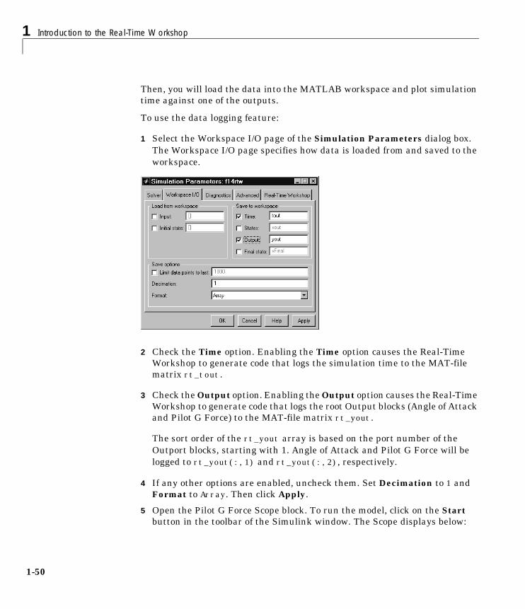
1 Introduction to the Real-Time Workshop
1-50
Then, you will load the data into the MATLAB workspace and plot simulationtime against one of the outputs.
To use the data logging feature:
1 Select the Workspace I/O page of the Simulation Parameters dialog box.The Workspace I/O page specifies how data is loaded from and saved to theworkspace.
2 Check the Time option. Enabling the Time option causes the Real-TimeWorkshop to generate code that logs the simulation time to the MAT-filematrix rt_tout.
3 Check the Output option. Enabling the Output option causes the Real-TimeWorkshop to generate code that logs the root Output blocks (Angle of Attackand Pilot G Force) to the MAT-file matrix rt_yout.
The sort order of the rt_yout array is based on the port number of theOutport blocks, starting with 1. Angle of Attack and Pilot G Force will belogged to rt_yout(:,1) and rt_yout(:,2), respectively.
4 If any other options are enabled, uncheck them. Set Decimation to 1 andFormat to Array. Then click Apply.
5 Open the Pilot G Force Scope block. To run the model, click on the Startbutton in the toolbar of the Simulink window. The Scope displays below:

Getting Started: Basic Concepts and Tutorials
1-51
6 Verify that the simulation time and Pilot G Force outputs have beencorrectly saved to the workspace by plotting simulation time versus Pilot GForce.
plot(tout,yout(:,2))
The resultant plot is shown below.
1 Introduction to the Real-Time Workshop
1-52
7 The f14rtw program must be rebuilt, because you have changed the modelby enabling data logging. Select Build Model from the Real-TimeWorkshop submenu of the Tools menu in the Simulink window. This is analternative way to start the Real-Time Workshop build process. It isidentical to using Build button in the Simulation Parameters dialog box.
8 When the build concludes, run the executable with the command
!f14rtw
9 The program now produces two message lines, indicating that the MAT-filehas been written.
**starting the model** ** created f14rtw.mat **
10 Clear the workspace, load the MAT-file data, and look at the workspacevariables.
clearload f14rtw.matwhos
11 Observe that the variables rt_tout (time) and rt_yout (G Force and Angleof Attack) have been loaded from the file. Plot G Force as a function of time.
plot(rt_tout,rt_yout(:,2))
12 The plot should appear identical to the plot you produced in step 5 above.
Tutorial 3: Code ValidationIn this tutorial, the code generated from the f14rtw model is validated againstthe model. The code is validated by capturing and comparing data from runs ofthe Simulink model and the generated program.
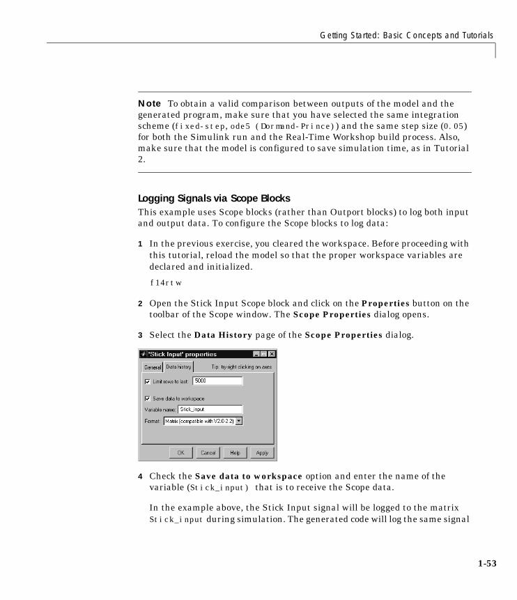
Getting Started: Basic Concepts and Tutorials
1-53
Note To obtain a valid comparison between outputs of the model and thegenerated program, make sure that you have selected the same integrationscheme (fixed-step, ode5 (Dormand-Prince)) and the same step size (0.05)for both the Simulink run and the Real-Time Workshop build process. Also,make sure that the model is configured to save simulation time, as in Tutorial2.
Logging Signals via Scope BlocksThis example uses Scope blocks (rather than Outport blocks) to log both inputand output data. To configure the Scope blocks to log data:
1 In the previous exercise, you cleared the workspace. Before proceeding withthis tutorial, reload the model so that the proper workspace variables aredeclared and initialized.
f14rtw
2 Open the Stick Input Scope block and click on the Properties button on thetoolbar of the Scope window. The Scope Properties dialog opens.
3 Select the Data History page of the Scope Properties dialog.
4 Check the Save data to workspace option and enter the name of thevariable (Stick_input) that is to receive the Scope data.
In the example above, the Stick Input signal will be logged to the matrixStick_input during simulation. The generated code will log the same signal
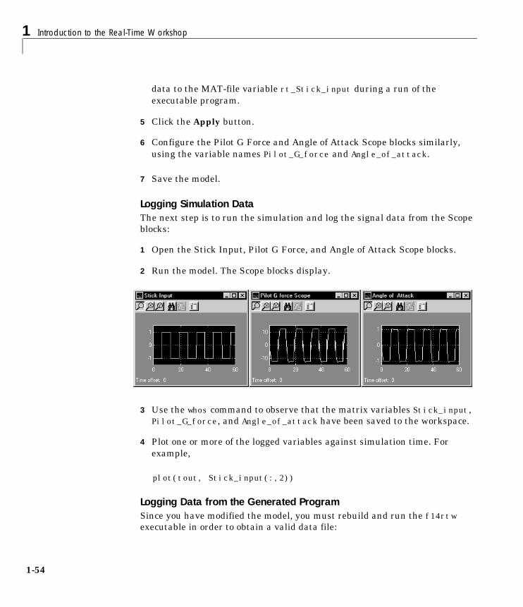
1 Introduction to the Real-Time Workshop
1-54
data to the MAT-file variable rt_Stick_input during a run of theexecutable program.
5 Click the Apply button.
6 Configure the Pilot G Force and Angle of Attack Scope blocks similarly,using the variable names Pilot_G_force and Angle_of_attack.
7 Save the model.
Logging Simulation DataThe next step is to run the simulation and log the signal data from the Scopeblocks:
1 Open the Stick Input, Pilot G Force, and Angle of Attack Scope blocks.
2 Run the model. The Scope blocks display.
3 Use the whos command to observe that the matrix variables Stick_input, Pilot_G_force, and Angle_of_attack have been saved to the workspace.
4 Plot one or more of the logged variables against simulation time. Forexample,
plot(tout, Stick_input(:,2))
Logging Data from the Generated ProgramSince you have modified the model, you must rebuild and run the f14rtwexecutable in order to obtain a valid data file:

Getting Started: Basic Concepts and Tutorials
1-55
1 Select Build Model from the Real-Time Workshop submenu of the Toolsmenu in the Simulink window.
2 When the build completes, run the stand-alone program from MATLAB.
!f14rtw
3 Load the data file f14rtw.mat and observe the workspace variables.
load f14rtwwhos
The data loaded from the MAT-file will include rt_Pilot_G_force,rt_Angle_of_attack, rt_Stick_input, and rt_tout.
4 You can now use MATLAB to plot the three workspace variables as afunction of time.
plot(rt_tout,rt_Stick_input(:,2))figureplot(rt_tout,rt_Pilot_G_force(:,2))figureplot(rt_tout,rt_Angle_of_attack(:,2))
Comparing Results of the Simulation and the Generated ProgramYour Simulink simulations and the generated code should produce nearlyidentical output.

1 Introduction to the Real-Time Workshop
1-56
You have now obtained data from a Simulink run of the model, and from a runof the program generated from the model. It is a simple matter to compare thef14rtw model output to the results achieved by the Real-Time Workshop.
Comparing Angle_of_attack (simulation output) to rt_Angle_of_attack (generated program output) produces
max(abs(rt_Angle_of_attack-Angle_of_attack))ans = 1.0e-015 * 0 0.4441
Comparing Pilot_G_force (simulation output) to rt_Pilot_G_force (generated program output) produces
max(abs(rt_Pilot_G_force-Pilot_G_force))ans = 1.0e-013 * 0 0.7283
So overall agreement is within 10-13. This slight error can be caused by manyfactors, including:
• Different compiler optimizations
• Statement ordering
• Run-time libraries
For example, a function such as sin(2.0)may return a slightly different value,depending on which C library you are using.
For the same reasons, your comparison results may not be identical to thoseabove.
Tutorial 4: A First Look at Generated CodeIn this tutorial, you examine code generated from a from a simple model, toobserve the effects of one of the many code optimization features available inthe Real-Time Workshop.
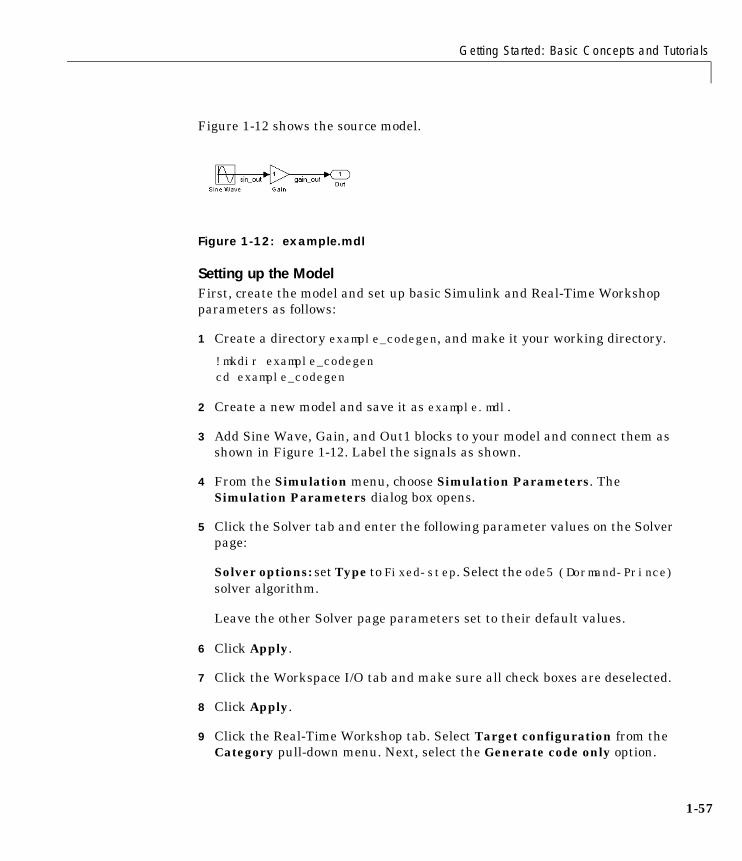
Getting Started: Basic Concepts and Tutorials
1-57
Figure 1-12 shows the source model.
Figure 1-12: example.mdl
Setting up the ModelFirst, create the model and set up basic Simulink and Real-Time Workshopparameters as follows:
1 Create a directory example_codegen, and make it your working directory.
!mkdir example_codegencd example_codegen
2 Create a new model and save it as example.mdl.
3 Add Sine Wave, Gain, and Out1 blocks to your model and connect them asshown in Figure 1-12. Label the signals as shown.
4 From the Simulation menu, choose Simulation Parameters. TheSimulation Parameters dialog box opens.
5 Click the Solver tab and enter the following parameter values on the Solverpage:
Solver options: set Type to Fixed-step. Select the ode5 (Dormand-Prince)solver algorithm.
Leave the other Solver page parameters set to their default values.
6 Click Apply.
7 Click the Workspace I/O tab and make sure all check boxes are deselected.
8 Click Apply.
9 Click the Real-Time Workshop tab. Select Target configuration from theCategory pull-down menu. Next, select the Generate code only option.
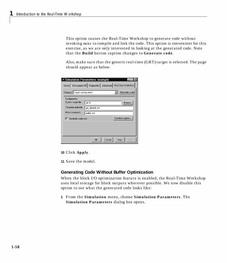
1 Introduction to the Real-Time Workshop
1-58
This option causes the Real-Time Workshop to generate code withoutinvoking make to compile and link the code. This option is convenient for thisexercise, as we are only interested in looking at the generated code. Notethat the Build button caption changes to Generate code.
Also, make sure that the generic real-time (GRT) target is selected. The pageshould appear as below.
10 Click Apply.
11 Save the model.
Generating Code Without Buffer OptimizationWhen the block I/O optimization feature is enabled, the Real-Time Workshopuses local storage for block outputs wherever possible. We now disable thisoption to see what the generated code looks like:
1 From the Simulation menu, choose Simulation Parameters. TheSimulation Parameters dialog box opens.
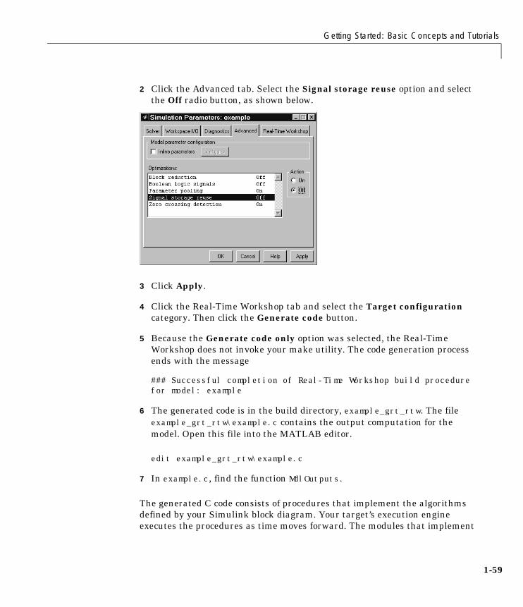
Getting Started: Basic Concepts and Tutorials
1-59
2 Click the Advanced tab. Select the Signal storage reuse option and selectthe Off radio button, as shown below.
3 Click Apply.
4 Click the Real-Time Workshop tab and select the Target configurationcategory. Then click the Generate code button.
5 Because the Generate code only option was selected, the Real-TimeWorkshop does not invoke your make utility. The code generation processends with the message
### Successful completion of Real-Time Workshop build procedure for model: example
6 The generated code is in the build directory, example_grt_rtw. The fileexample_grt_rtw\example.c contains the output computation for themodel. Open this file into the MATLAB editor.
edit example_grt_rtw\example.c
7 In example.c, find the function MdlOutputs.
The generated C code consists of procedures that implement the algorithmsdefined by your Simulink block diagram. Your target’s execution engineexecutes the procedures as time moves forward. The modules that implement

1 Introduction to the Real-Time Workshop
1-60
the execution engine and other capabilities are referred to collectively as therun-time interface modules.
In our example, the generated MdlOutputs function implements the actualalgorithm for multiplying a sine wave by a gain. The MdlOutputs functioncomputes the model’s block outputs. The run-time interface must callMdlOutputs at every time step.
With buffer optimizations turned off, MdlOutputs assigns buffers to each blockinput and output. These buffers (rtB.sin_out, rtB.gain_out) are members ofa global data structure, rtB. The code is shown below.
void MdlOutputs(int_T tid){ /* Sin Block: <Root>/Sine Wave */ rtB.sin_out = rtP.Sine_Wave_Amp * sin(rtP.Sine_Wave_Freq * ssGetT(rtS) + rtP.Sine_Wave_Phase); /* Gain Block: <Root>/Gain */ rtB.gain_out = rtB.sin_out * rtP.Gain_Gain; /* Outport Block: <Root>/Out1 */ rtY.Out1 = rtB.gain_out;}
We now turn buffer optimization on and observe how it improves the code.
Generating Code with Buffer OptimizationEnable buffer optimization and re-generate the code as follows:
1 From the Simulation menu, choose Simulation Parameters. TheSimulation Parameters dialog box opens.
2 Click the Advanced tab. Select the Signal storage reuse option and selectthe On radio button.
3 Click Apply.
4 Click the Real-Time Workshop tab. Select General code generationoptions from the Category pull-down menu.
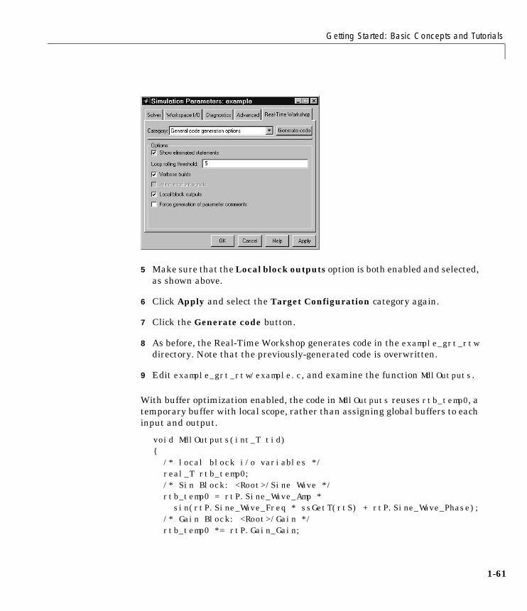
Getting Started: Basic Concepts and Tutorials
1-61
5 Make sure that the Local block outputs option is both enabled and selected,as shown above.
6 Click Apply and select the Target Configuration category again.
7 Click the Generate code button.
8 As before, the Real-Time Workshop generates code in the example_grt_rtwdirectory. Note that the previously-generated code is overwritten.
9 Edit example_grt_rtw/example.c, and examine the function MdlOutputs.
With buffer optimization enabled, the code in MdlOutputs reuses rtb_temp0, atemporary buffer with local scope, rather than assigning global buffers to eachinput and output.
void MdlOutputs(int_T tid){ /* local block i/o variables */
real_T rtb_temp0; /* Sin Block: <Root>/Sine Wave */ rtb_temp0 = rtP.Sine_Wave_Amp * sin(rtP.Sine_Wave_Freq * ssGetT(rtS) + rtP.Sine_Wave_Phase); /* Gain Block: <Root>/Gain */ rtb_temp0 *= rtP.Gain_Gain;

1 Introduction to the Real-Time Workshop
1-62
/* Outport Block: <Root>/Out1 */ rtY.Out1 = rtb_temp0;}
This code is more efficient in terms of memory usage. The efficiencyimprovement gained by enabling Local block outputs would be moresignificant in a large model with many signals.
Note that, by default, Local block outputs is enabled. Chapter 3, “CodeGeneration and the Build Process” contains details on this and other codegeneration options.
For further information on the structure and execution of model.c files, referto Chapter 6, “Program Architecture.”
Where to Find Information in This Manual
1-63
Where to Find Information in This ManualThe list below will guide you to information relevant to your development tasksand interests.
Single- and Multitasking Code GenerationThe Real-Time Workshop fully supports single- and multitasking codegeneration. See Chapter 6, “Program Architecture” and Chapter 7, “Modelswith Multiple Sample Rates” for a complete description.
Customizing Generated CodeThe Real-Time Workshop Custom Code library supports customization of thegenerated code. See Chapter 14, “Custom Code Blocks” for a description of thislibrary.
An alternative approach to customizing generated code is to modify TargetLanguage Compiler (TLC) files. The Target Language Compiler is aninterpreted language that translates Simulink models into C code. Using theTarget Language Compiler, you can direct the code generation process.
There are two TLC files, hookslib.tlc and cachelib.tlc, that containfunctions you can use to customize Real-Time Workshop generated code. Seethe Target Language Compiler Reference Guide for more information aboutthese TLC files. See also the source code, located in matlabroot/rtw/c/tlc.
Optimizing Generated CodeThe default code generation settings are generic for flexible rapid prototypingsystems. The penalty for this flexibility is code that is less than optimal. Thereare several optimization techniques that you can use to minimize the sourcecode size and memory usage once you have a model that meets yourrequirements.
See Chapter 3, “Code Generation and the Build Process” and Chapter 8,“Optimizing the Model for Code Generation” for details on code optimizationtechniques available for all target configurations.
Chapter 9, “Real-Time Workshop Embedded Coder” contains informationabout optimization specifically for embedded code.

1 Introduction to the Real-Time Workshop
1-64
Validating Generated CodeUsing the Real-Time Workshop data logging features, you can create anexecutable that runs on your workstation and creates a data file. You can thencompare the results of your program with the results of running an equivalentSimulink simulation.
For more information on how to validate Real-Time Workshop generated code,see “Workspace I/O Options and Data Logging” on page 3-18. See also “Tutorial2: Data Logging” and “Tutorial 3: Code Validation” in this chapter.
Incorporating Generated Code into Larger SystemsIf your Real-Time Workshop generated code is intended to function within anexisting code base (for example, if you want to use the generated code as aplug-in function), you should use the Real-Time Workshop Embedded Coder.Chapter 9, “Real-Time Workshop Embedded Coder” documents the entrypoints and header files you will need to interface your code to Real-TimeWorkshop Embedded Coder generated code.
Incorporating Your Code into Generated CodeTo interface your hand-written code with Real-Time Workshop generated code,you can use an S-function wrapper. See the Writing S-Functions manual formore information.
Creating and Communicating with Device DriversS-functions provide a flexible method for communicating with device drivers.See Chapter 17, “Targeting Real-Time Systems” for a description of how tobuild device drivers. Also, for a complete discussion of S-functions, see theWriting S-Functions manual.
Code TracingThe Real-Time Workshop includes special tags throughout the generated codethat make it easy to trace generated code back to your Simulink model. See“Tracing Generated Code Back to Your Simulink Model” on page 3-28 for moreinformation about this feature.
Where to Find Information in This Manual
1-65
Automatic Build ProcedureUsing the Real-Time Workshop, you can generate code with the push of abutton. The automatic build procedure, initiated by a single mouse click,generates code, a makefile, and optionally compiles (or cross-compiles) anddownloads a program. See “Automatic Program Building” on page 2-12 for anoverview, and Chapter 3, “Code Generation and the Build Process” for completedetails.
Parameter TuningParameter tuning enables you to change block parameters while a generatedprogram runs, thus avoiding recompiling the generated code. The Real-TimeWorkshop supports parameter tuning in four different environments:
• External mode: You can tune parameters from Simulink while running thegenerated code on a target processor. See Chapter 5, “External Mode” forinformation on this mode.
• External C application program interface (API): You can write your own CAPI interface for parameter tuning using support files provided by TheMathWorks. See Chapter 17, “Targeting Real-Time Systems” for moreinformation.
• Rapid simulation: You can use the Rapid Simulation Target (rsim) in batchmode to provide fast simulations for performing parametric studies.Although this is not an on-the-fly application of parameter tuning, it isnevertheless a useful way to evaluate a model. This mode is also useful forMonte Carlo simulation. See Chapter 11, “Real-Time Workshop RapidSimulation Target” for further information.
• Simulink: Prior to generating real-time code, you can tune parameterson-the-fly in your Simulink model.
See also “Interfacing Signals and Parameters” on page 1-66.
Monitoring Signals and Logging DataThere are several ways to monitor signals and data in the Real-TimeWorkshop:
• External mode: You can monitor and log signals from an externallyexecuting program via Scope blocks and several other types of external mode
1 Introduction to the Real-Time Workshop
1-66
compatible blocks. See “External Signal & Triggering Dialog Box” on page5-24 for a discussion of this method.
• External C application program interface (API): You can write your own CAPI for signal monitoring using support files provided by The MathWorks.See Chapter 17, “Targeting Real-Time Systems” for more information.
• MAT-file logging: You can use a MAT-file to log data from the generatedexecutable. See “Workspace I/O Options and Data Logging” on page 3-18 formore information.
• Simulink: You can use any of Simulink’s data logging capabilities.
Interfacing Signals and Parameters You can interface signals and parameters in your model to hand-written codeby specifying the storage declarations of signals and parameters. For moreinformation, see:
• “Parameters: Storage, Interfacing, and Tuning” on page 3-51
• “Signals: Storage, Optimization, and Interfacing” on page 3-65
• “Interfacing Parameters and Signals” on page 17-65
Sample ImplementationsThe Real-Time Workshop provides sample implementations that illustrate thedevelopment of real-time programs under DOS and Tornado, as well as genericreal-time programs under Windows and UNIX.
These sample implementations are located in the following directories:
• matlabroot/rtw/c/grt: Generic real-time examples
• matlabroot/rtw/c/dos: DOS examples
• matlabroot/rtw/c/tornado: Tornado examples
2
Technical Overview
The Rapid Prototyping Process . . . . . . . . . . . . 2-2Key Aspects of Rapid Prototyping . . . . . . . . . . . . 2-2Rapid Prototyping for Digital Signal Processing . . . . . . 2-5Rapid Prototyping for Control Systems . . . . . . . . . . 2-6
Open Architecture of the Real-Time Workshop . . . . . 2-8
Automatic Program Building . . . . . . . . . . . . . 2-12Steps in the Build Process . . . . . . . . . . . . . . . 2-13
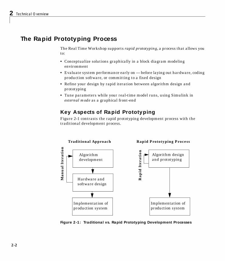
2 Technical Overview
2-2
The Rapid Prototyping ProcessThe Real Time Workshop supports rapid prototyping, a process that allows youto:
• Conceptualize solutions graphically in a block diagram modelingenvironment
• Evaluate system performance early on — before laying out hardware, codingproduction software, or committing to a fixed design
• Refine your design by rapid iteration between algorithm design andprototyping
• Tune parameters while your real-time model runs, using Simulink inexternal mode as a graphical front-end
Key Aspects of Rapid PrototypingFigure 2-1 contrasts the rapid prototyping development process with thetraditional development process.
Figure 2-1: Traditional vs. Rapid Prototyping Development Processes
Traditional Approach Rapid Prototyping ProcessR
apid
Iter
atio
n
Man
ual
Iter
atio
n
Algorithmdevelopment
Algorithm designand prototyping
Hardware andsoftware design
Implementation ofproduction system
Implementation ofproduction system
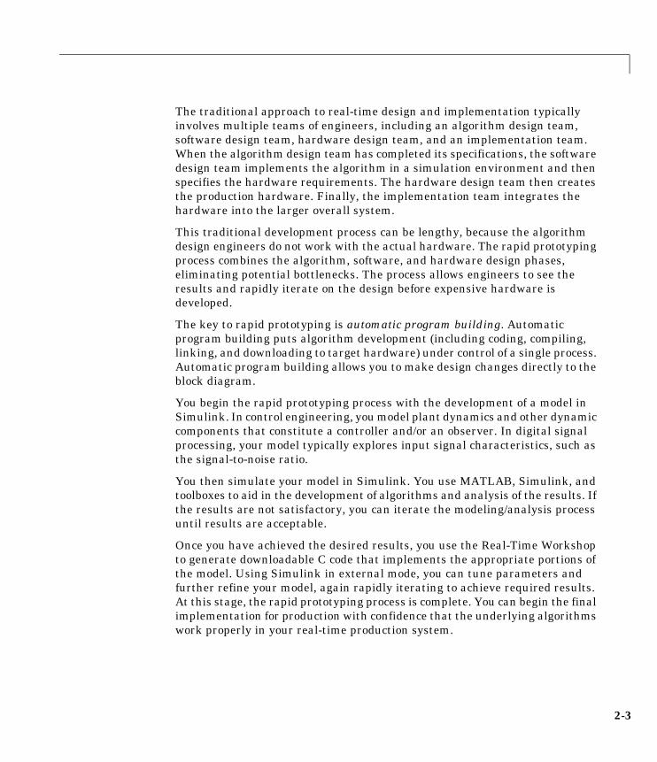
2-3
The traditional approach to real-time design and implementation typicallyinvolves multiple teams of engineers, including an algorithm design team,software design team, hardware design team, and an implementation team.When the algorithm design team has completed its specifications, the softwaredesign team implements the algorithm in a simulation environment and thenspecifies the hardware requirements. The hardware design team then createsthe production hardware. Finally, the implementation team integrates thehardware into the larger overall system.
This traditional development process can be lengthy, because the algorithmdesign engineers do not work with the actual hardware. The rapid prototypingprocess combines the algorithm, software, and hardware design phases,eliminating potential bottlenecks. The process allows engineers to see theresults and rapidly iterate on the design before expensive hardware isdeveloped.
The key to rapid prototyping is automatic program building. Automaticprogram building puts algorithm development (including coding, compiling,linking, and downloading to target hardware) under control of a single process.Automatic program building allows you to make design changes directly to theblock diagram.
You begin the rapid prototyping process with the development of a model inSimulink. In control engineering, you model plant dynamics and other dynamiccomponents that constitute a controller and/or an observer. In digital signalprocessing, your model typically explores input signal characteristics, such asthe signal-to-noise ratio.
You then simulate your model in Simulink. You use MATLAB, Simulink, andtoolboxes to aid in the development of algorithms and analysis of the results. Ifthe results are not satisfactory, you can iterate the modeling/analysis processuntil results are acceptable.
Once you have achieved the desired results, you use the Real-Time Workshopto generate downloadable C code that implements the appropriate portions ofthe model. Using Simulink in external mode, you can tune parameters andfurther refine your model, again rapidly iterating to achieve required results.At this stage, the rapid prototyping process is complete. You can begin the finalimplementation for production with confidence that the underlying algorithmswork properly in your real-time production system.
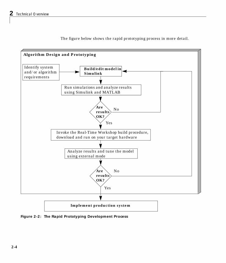
2 Technical Overview
2-4
The figure below shows the rapid prototyping process in more detail.
Figure 2-2: The Rapid Prototyping Development Process
Identify systemand/ or algorithmrequirements
Build/edit model inSimulink
Run simulations and analyze resultsusing Simulink and MATLAB
AreresultsOK?
Invoke the Real-Time Workshop build procedure,download and run on your target hardware
Analyze results and tune the modelusing external mode
Implement production system
No
Yes
NoAreresultsOK?
Yes
Algorithm Design and Prototyping
2-5
This highly productive development cycle is possible because the Real-TimeWorkshop is closely tied to MATLAB and Simulink. Each package contributesto the design of your application:
• MATLAB: Provides design, analysis, and data visualization tools.
• Simulink: Provides system modeling, simulation, and validation.
• Real-Time Workshop: Generates C or Ada code from Simulink model;provides framework for running generated code in real-time, tuningparameters, and viewing real-time data.
Rapid Prototyping for Digital Signal ProcessingThe first step in the rapid prototyping process for digital signal processing is toconsider the kind and quality of the data to be worked on, and to relate it to thesystem requirements. Typically this includes examining the signal-to-noiseratio, distortion, and other characteristics of the incoming signal, and relatingthem to algorithm and design choices.
System Simulation and Algorithm DesignIn the rapid prototyping process, the block diagram plays two roles inalgorithm development. The block diagram helps to identify processingbottlenecks, and to optimize the algorithm or system architecture. The blockdiagram also functions as a high-level system description.That is, the diagramprovides a hierarchical framework for evaluating the behavior and accuracy ofalternative algorithms under a range of operating conditions.
Analyzing Results, Parameter Tuning, and Signal Monitoring Using External ModeAfter creating an algorithm (or a set of candidate algorithms), the next stage isto consider architectural and implementation issues. These includecomplexity, speed, and accuracy. In a conventional development environment,this would mean running the algorithm and recoding it in C or in a hardwaredesign and simulation package.
Simulink’s external mode allows you to change parameters interactively, whileyour signal processing algorithms execute in real time on the target hardware.After building the executable and downloading it to your hardware, you tune(modify) block parameters in Simulink. Simulink automatically downloads the

2 Technical Overview
2-6
new values to the hardware. You can monitor the effects of your parameterchanges by simply connecting Scope blocks to signals that you want to observe.
Rapid Prototyping for Control SystemsRapid prototyping for control systems is similar to digital signal processing,with one major difference. In control systems design, it is necessary to developa model of your plant prior to algorithm development in order to simulateclosed loop performance. Once your plant model is sufficiently accurate, therapid prototyping process for control system design continues in much thesame manner as digital signal processing design.
Rapid prototyping begins with developing block diagram plant models ofsufficient fidelity for preliminary system design and simulation. Oncesimulations show encouraging system performance, the controller blockdiagram is separated from the plant model and I/O device drivers are attached.Automatic code generation immediately converts the entire system to real-timeexecutable code. The executable can be automatically loaded onto targethardware, allowing the implementation of real-time control systems in a veryshort time.
Modeling Systems in SimulinkThe first step in the design process is development of a plant model. TheSimulink collection of linear and nonlinear components helps you to buildmodels involving plant, sensor, and actuator dynamics. Because Simulink iscustomizable, you can further simplify modeling by creating custom blocks andblock libraries from continuous- and discrete-time components.
Using the System Identification Toolbox, you can analyze test data to developan empirical plant model; or you can use the Symbolic Math Toolbox totranslate the equations of the plant dynamics into state-variable form.
Analysis of Simulation ResultsYou can use MATLAB and Simulink to analyze the results produced from amodel developed in the first step of the rapid prototyping process. At this stage,you can design and add a controller to your plant.
Algorithm Design and AnalysisFrom the block diagrams developed during the modeling stage, you can extractstate-space models through linearization techniques. These matrices can be
2-7
used in control system design. You can use the following toolboxes to facilitatecontrol system design, and work with the matrices that you derived:
• Control System Toolbox
• LMI Control Toolbox
• Model Predictive Control Toolbox
• Robust Control Toolbox
Once you have your controller designed, you can create a closed-loop system byconnecting it to the Simulink plant model. Closed-loop simulations allow youto determine how well the initial design meets performance requirements.
Once you have a satisfactory model, it is a simple matter to generate C codedirectly from the Simulink block diagram, compile it for the target processor,and link it with supplied or user-written application modules.
Analyzing Results, Parameter Tuning, and Signal MonitoringUsing External ModeYou can load output data from your program into MATLAB for analysis, ordisplay the data with third party monitoring tools. You can easily make designchanges to the Simulink model and then regenerate the C code.
Simulink’s external mode allows you to change parameters interactively, whileyour algorithms execute in real time on the target hardware. After building theexecutable and downloading it to your hardware, you tune (modify) blockparameters in Simulink. Simulink automatically downloads the new values tothe hardware. You can monitor the effects of your parameter changes by simplyconnecting Scope blocks to signals that you want to observe.
2 Technical Overview
2-8
Open Architecture of the Real-Time WorkshopThe Real-Time Workshop is an open system designed for use with a widevariety of operating environments and hardware types. There are many waysto modify and extend the key elements of Real-Time Workshop. Figure 2-3shows these elements.
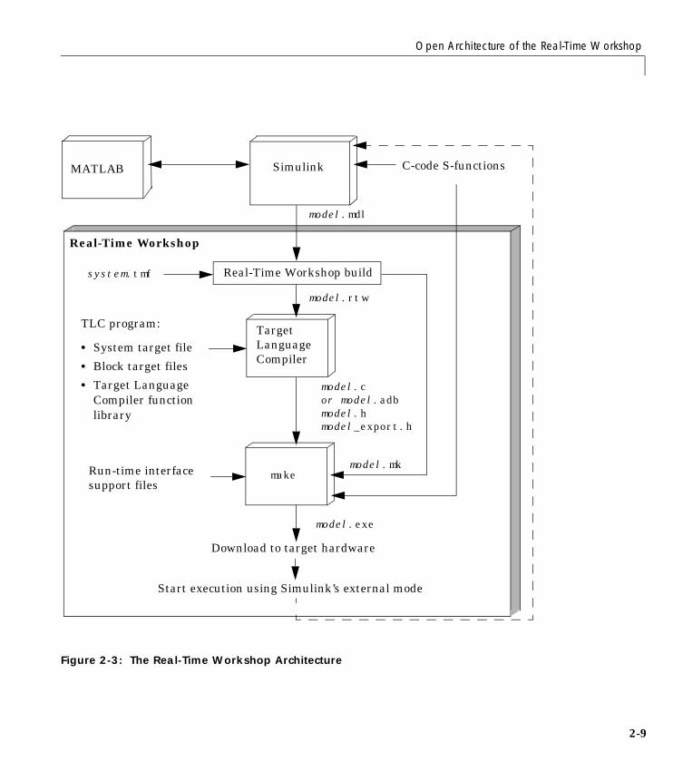
Open Architecture of the Real-Time Workshop
2-9
Figure 2-3: The Real-Time Workshop Architecture
MATLAB Simulink
Real-Time Workshop build
TargetLanguageCompiler
make
Real-Time Workshop
system.tmf
model.cor model.adbmodel.hmodel_export.h
TLC program:
• System target file
• Block target files
• Target LanguageCompiler functionlibrary
Run-time interfacesupport files
model.exe
Download to target hardware
model.mdl
C-code S-functions
Start execution using Simulink’s external mode
model.rtw
model.mk
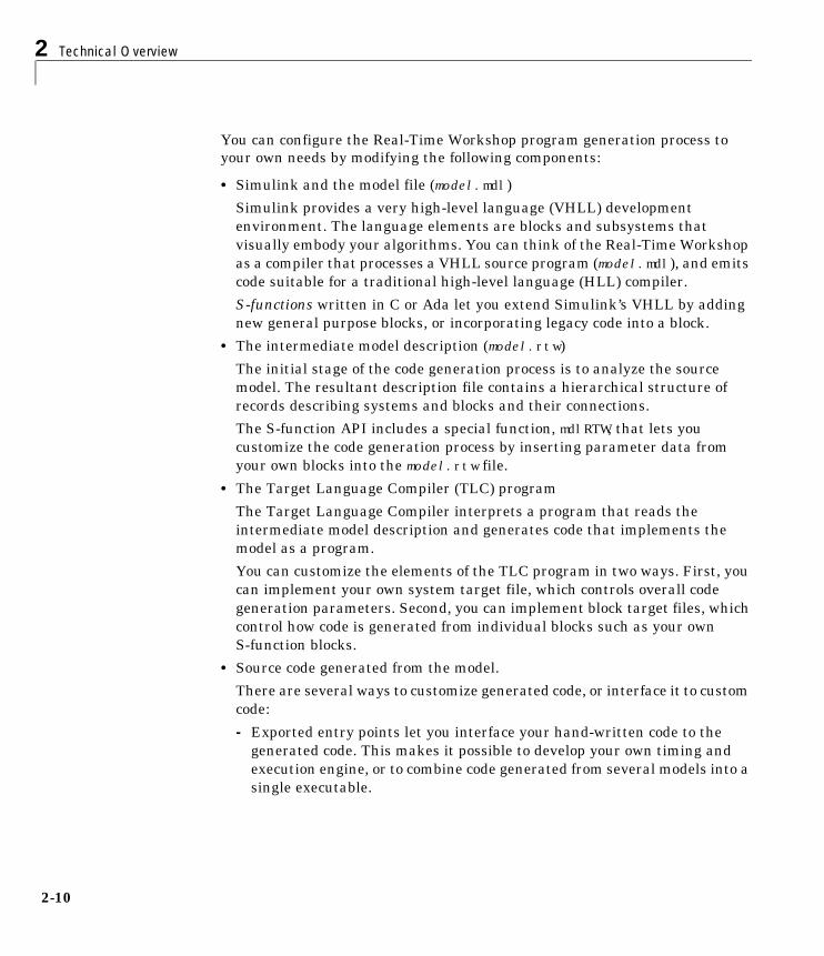
2 Technical Overview
2-10
You can configure the Real-Time Workshop program generation process toyour own needs by modifying the following components:
• Simulink and the model file (model.mdl)
Simulink provides a very high-level language (VHLL) developmentenvironment. The language elements are blocks and subsystems thatvisually embody your algorithms. You can think of the Real-Time Workshopas a compiler that processes a VHLL source program (model.mdl), and emitscode suitable for a traditional high-level language (HLL) compiler.
S-functions written in C or Ada let you extend Simulink’s VHLL by addingnew general purpose blocks, or incorporating legacy code into a block.
• The intermediate model description (model.rtw)
The initial stage of the code generation process is to analyze the sourcemodel. The resultant description file contains a hierarchical structure ofrecords describing systems and blocks and their connections.
The S-function API includes a special function, mdlRTW, that lets youcustomize the code generation process by inserting parameter data fromyour own blocks into the model.rtw file.
• The Target Language Compiler (TLC) program
The Target Language Compiler interprets a program that reads theintermediate model description and generates code that implements themodel as a program.
You can customize the elements of the TLC program in two ways. First, youcan implement your own system target file, which controls overall codegeneration parameters. Second, you can implement block target files, whichcontrol how code is generated from individual blocks such as your ownS-function blocks.
• Source code generated from the model.
There are several ways to customize generated code, or interface it to customcode:
- Exported entry points let you interface your hand-written code to thegenerated code. This makes it possible to develop your own timing andexecution engine, or to combine code generated from several models into asingle executable.
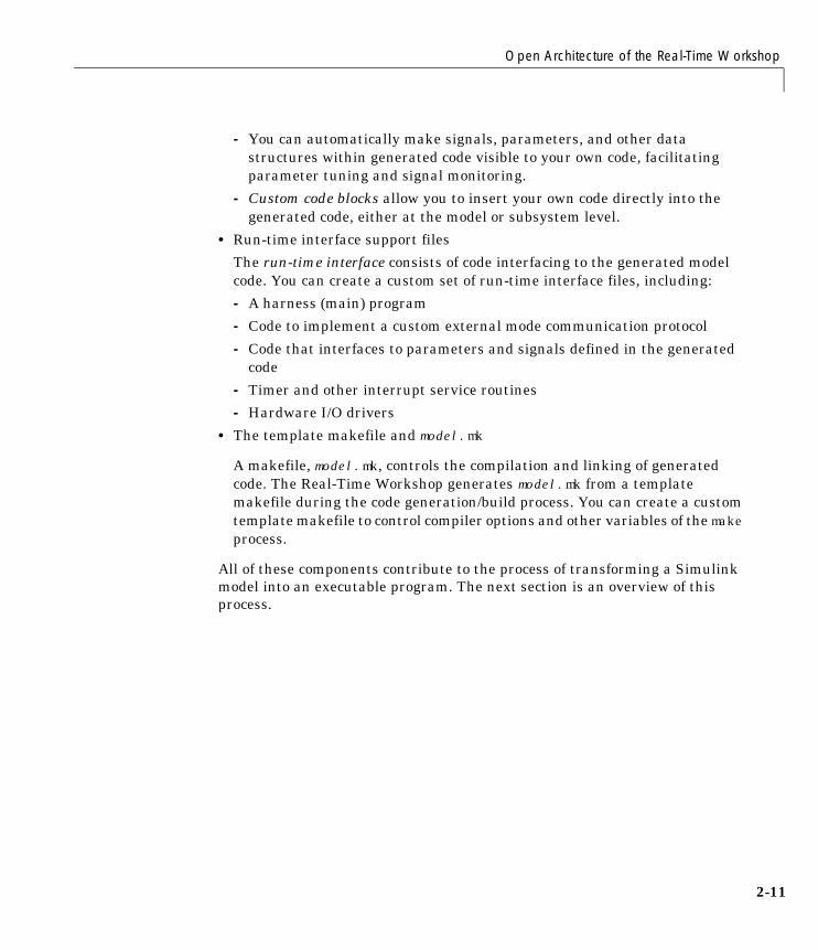
Open Architecture of the Real-Time Workshop
2-11
- You can automatically make signals, parameters, and other datastructures within generated code visible to your own code, facilitatingparameter tuning and signal monitoring.
- Custom code blocks allow you to insert your own code directly into thegenerated code, either at the model or subsystem level.
• Run-time interface support files
The run-time interface consists of code interfacing to the generated modelcode. You can create a custom set of run-time interface files, including:
- A harness (main) program
- Code to implement a custom external mode communication protocol
- Code that interfaces to parameters and signals defined in the generatedcode
- Timer and other interrupt service routines
- Hardware I/O drivers
• The template makefile and model.mk
A makefile, model.mk, controls the compilation and linking of generatedcode. The Real-Time Workshop generates model.mk from a templatemakefile during the code generation/build process. You can create a customtemplate makefile to control compiler options and other variables of the makeprocess.
All of these components contribute to the process of transforming a Simulinkmodel into an executable program. The next section is an overview of thisprocess.
2 Technical Overview
2-12
Automatic Program BuildingThe Real-Time Workshop automatic program building process createsprograms for real-time applications in a variety of host environments.Automatic program building uses the make utility to control the compilationand linking of generated source code.
A high-level M-file command controls the Real-Time Workshop build process.The default command, used with most targets, is make_rtw.
The build process consists of the following steps:
1 Analysis of the model and compilation of a model description file
2 Generation of code from the model by the Target Language Compiler
3 Generation of a makefile, customized for a given build
4 Creation of an executable program by the make utility under the control ofthe customized makefile
The shaded box in Figure 2-4 outlines these steps.
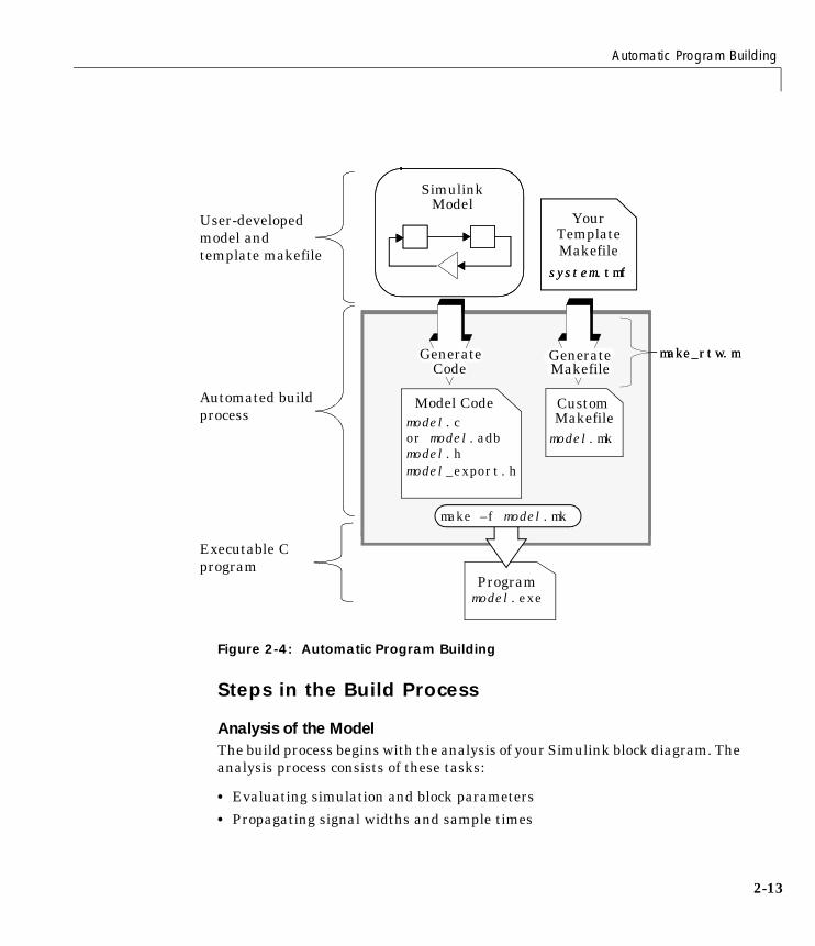
Automatic Program Building
2-13
Figure 2-4: Automatic Program Building
Steps in the Build Process
Analysis of the ModelThe build process begins with the analysis of your Simulink block diagram. Theanalysis process consists of these tasks:
• Evaluating simulation and block parameters
• Propagating signal widths and sample times
SimulinkModel
TemplateMakefile
Your
model.mk
GenerateCode
Generate
make –f mk
Model
c
CustomMakefile
Makefile
system.tmf
make_rtw.m
Code
h
model
model.mk
model.exeProgram
GenerateCode
Generate
make –f model.mk
Model Codemodel.c
CustomMakefile
Makefile
system.tmf
make_rtw.m
or model.adb
User-developedmodel andtemplate makefile
Automated buildprocess
Executable Cprogram
model.hmodel_export.h
2 Technical Overview
2-14
• Determining the execution order of blocks within the model
• Computing work vector sizes such as those used by S-functions (for moreinformation about work vectors, refer to the Writing S-Functions manual.)
During this phase, the Real-Time Workshop reads your model file (model.mdl)and compiles an intermediate representation of the model. This intermediatedescription is stored, in a language-independent format, in an ASCII filenamed model.rtw. The model.rtw file is the input to the next stage of the buildprocess.
model.rtw files are similar in format to Simulink model (.mdl) files. “Overviewof a model.rtw File” on page 2–17 explains the basic features of a .rtw file. Fora detailed description of the contents of model.rtw files, see the TargetLanguage Compiler Reference Guide.
Generation of Code by the Target Language CompilerIn the second stage of the build procedure, the Target Language Compilertransforms the intermediate model description stored in model.rtw intotarget-specific code.
The Target Language Compiler is an interpreted programming languagedesigned for the sole purpose of converting a model description into code. TheTarget Language Compiler executes a TLC program comprising several targetfiles (.tlc files). The TLC program specifies how to generate code from themodel, using the model.rtw file as input.
The TLC program consists of:
• The system target file
The system target file is the entry point or main file.
• Block target files
For each block in a Simulink model, there is a block target file that specifieshow to translate that block into target-specific code.
• The Target Language Compiler function library
The Target Language Compiler function library contains functions thatsupport the code generation process.
The Target Language Compiler begins by reading in the model.rtw file. It thencompiles and executes the commands in the target files — first the system
Automatic Program Building
2-15
target file, then the individual block target files. The output of the TargetLanguage Compiler is a source code version of the Simulink block diagram.
Generation of the Customized MakefileThe third step in the build procedure is to generate a customized makefile,model.mk. The generated makefile instructs the make utility to compile and linksource code generated from the model, as well as any required harnessprogram, libraries, or user-provided modules.
The Real-Time Workshop creates model.mk from a system template makefile,system.tmf. The system template makefile is designed for your targetenvironment. The template makefile allows you to specify compilers, compileroptions, and additional information used during the creation of the executable.
The model.mk file is created by copying the contents of system.tmf andexpanding tokens that describe your model’s configuration.
The Real-Time Workshop provides many system template makefiles,configured for specific target environments and development systems. “TheSystem Target File Browser” on page 3-34 lists all template makefiles that arebundled with the Real-Time Workshop.
You can fully customize your build process by modifying an existing templatemakefile or providing your own template makefile.
Creation of the ExecutableCreation of an executable program is the final stage of the build process. Thisstage is optional, as illustrated in Figure 2-5.
If you are targeting a system such as an embedded microcontroller or a DSPboard, you can choose to generate only source code. You can then cross compileyour code and download it to your target hardware. “Making an Executable” inChapter 3 discusses the options that control whether or not the build createsan executable.
The creation of the executable, if enabled, takes place after the model.mk filehas been created. At this point, the build process invokes the make utility,which in turn runs the compiler. To avoid unnecessary recompilation of C files,the make utility performs date checking on the dependencies between the objectand C files; only out-of-date source files are compiled.
Optionally, make can also download the executable to your target hardware.
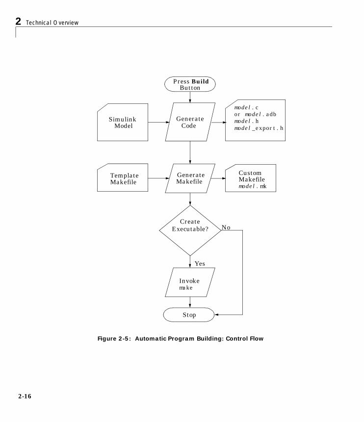
2 Technical Overview
2-16
Figure 2-5: Automatic Program Building: Control Flow
CustomGenerateMakefile
Press BuildButton
CreateExecutable? No
Invoke
Yes
GenerateCode
TemplateMakefile
SimulinkModel
Makefilemodel.mk
make
model.cor model.adbmodel.hmodel_export.h
Stop

Automatic Program Building
2-17
Summary of Files Created by the Build ProcedureThe following is a list of the main of the model.* files created during the codegeneration and build process. Each performs a specific function in theReal-Time Workshop. Depending on code generation options, other files mayalso be created by the build process.
• model.mdl, created by Simulink, is analogous to a high-level programminglanguage source file.
• model.rtw, generated by the Real-Time Workshop build process, isanalogous to the object file created from a high-level language sourceprogram.
• model.c, generated by the Target Language Compiler, is the C source codecorresponding to the model.mdl file.
• model.h, generated by the Target Language Compiler, is a header file thatmaps the links between blocks in the model.
• model_export.h, generated by the Target Language Compiler, is a headerfile that contains exported signal, parameter, and function symbols.
• model.mk, generated by the Real-Time Workshop build process, is thecustomized makefile used to build an executable.
• model.exe (on PC) or model (on UNIX), is an executable program, createdunder control of the make utility by your development system.
Overview of a model.rtw FileThis section examines the basic features of a model.rtw file. The .rtw fileshown is generated from the source model shown below.
This model is saved in a file called example.mdl. The Real-Time Workshopgenerates example.rtw., an ASCII file. The example.rtw file consists ofparameter name/parameter value pairs, stored in a hierarchical structureconsisting of records.
1
OutSine Wave
1
Gain
sin_out gain_out
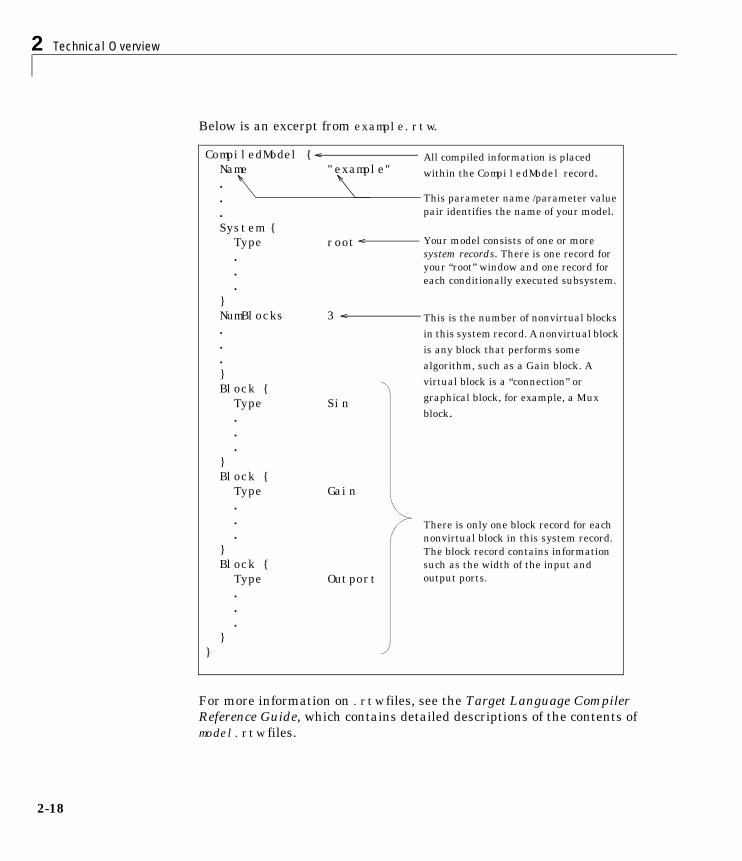
2 Technical Overview
2-18
Below is an excerpt from example.rtw.
For more information on .rtw files, see the Target Language CompilerReference Guide, which contains detailed descriptions of the contents ofmodel.rtw files.
CompiledModel {Name "example"...System {Type root...
}NumBlocks 3...}Block {Type Sin...
}Block {Type Gain...
}Block {Type Outport...
}}
All compiled information is placedwithin the CompiledModel record.
This parameter name /parameter valuepair identifies the name of your model.
Your model consists of one or moresystem records. There is one record foryour “root” window and one record foreach conditionally executed subsystem.
This is the number of nonvirtual blocksin this system record. A nonvirtual blockis any block that performs somealgorithm, such as a Gain block. Avirtual block is a “connection” orgraphical block, for example, a Muxblock.
There is only one block record for eachnonvirtual block in this system record.The block record contains informationsuch as the width of the input andoutput ports.
3Code Generation and theBuild Process
Introduction . . . . . . . . . . . . . . . . . . . . 3-2
Overview of the Real-Time Workshop User Interface . . . 3-4
Simulation Parameters and Code Generation . . . . . . 3-17
Selecting a Target Configuration . . . . . . . . . . . 3-34
Nonvirtual Subsystem Code Generation . . . . . . . . 3-41
Generating Code and Executables from Subsystems . . . 3-49
Parameters: Storage, Interfacing, and Tuning . . . . . . 3-51
Signals: Storage, Optimization, and Interfacing . . . . . 3-65
Simulink Data Objects and Code Generation . . . . . . 3-79
Configuring the Generated Code via TLC . . . . . . . . 3-93
Making an Executable . . . . . . . . . . . . . . . . 3-97
Directories Used in the Build Process . . . . . . . . . 3-98
Choosing and Configuring Your Compiler . . . . . . . 3-99
Template Makefiles and Make Options . . . . . . . . 3-102
3 Code Generation and the Build Process
3-2
IntroductionChapter 2, “Technical Overview” introduced code generation and the buildprocess. This chapter covers these topics in detail.
The Real-Time Workshop page of the Simulation Parameters dialog enablesyou to control most aspects of the code generation and build process. The firstsection of this chapter,“Overview of the Real-Time Workshop User Interface”on page 3-4, introduces the features controlled by the Real-Time Workshoppage.
The sections that follow concern the code generation phase of the build process:
• “Simulation Parameters and Code Generation” on page 3-17 discusses howoptions on the Simulink Solver, Workspace I/O, Diagnostics, and Advancedpages interact with code generation. These options include choice of single-or multitasking execution, and several methods of logging data to MAT-files.
The section also illustrates how to use tags in the generated code to traceback to the blocks that generated the code.
The section ends with a discussion of “Other Interactions Between Simulinkand the Real-Time Workshop” such as sample time propagation and order ofexecution of blocks.
• “Selecting a Target Configuration” on page 3-34 illustrates the use of theSystem Target File Browser, and summarizes the target configurations thatyou can access through the browser.
• “Nonvirtual Subsystem Code Generation” on page 3-41 describes generationof separate code modules from nonvirtual subsystems.
• “Generating Code and Executables from Subsystems” on page 3-49 describeshow to generate and build a stand-alone executable from a subsystem.
• “Parameters: Storage, Interfacing, and Tuning” on page 3-51 documents howto generate storage declarations in order to export and import modelparameters to and from user-written code.
• “Signals: Storage, Optimization, and Interfacing” on page 3-65 documentshow signal storage optimizations work, and how to generate storagedeclarations in order to export and import model signals to and fromuser-written code.
3-3
• “Simulink Data Objects and Code Generation” on page 3-79 documents howto represent and store signals and parameters in Simulink data objects, andhow code is generated from these object.
The remaining sections cover the make (post-code generation) part of the buildprocess:
• “Making an Executable” on page 3-97 documents options that controlwhether or not an executable is created during the build process.
• “Directories Used in the Build Process” on page 3-98 documents the outputdirectories used and/or created during the build process.
• “Choosing and Configuring Your Compiler” on page 3-99 discusses theinstallation of a compiler and choice of a template makefile appropriate foruse with your compiler.
• “Template Makefiles and Make Options” on page 3-102 includes a summaryof available template makefiles and make command options.
3 Code Generation and the Build Process
3-4
Overview of the Real-Time Workshop User InterfaceMany parameters and options affect the way that Real-Time Workshopgenerates code from your model and builds an executable. To set theseparameters and options, you interact with the pages of the SimulationParameters dialog box.
The Simulink Solver, Workspace I/O, Diagnostics, and Advanced pages affectboth the behavior of the model in simulation, and the code generated from themodel. “Simulation Parameters and Code Generation” on page 3-17 discusseshow Simulink settings affect the code generation process.
The Real-Time Workshop page lets you set parameters that directly affect codegeneration and optimization. You also initiate and control the build processfrom the Real-Time Workshop page.
Using the Real-Time Workshop PageThere are two ways to open the Real-Time Workshop page:
• From the Simulation menu, choose Simulation Parameters. When theSimulation Parameters dialog box opens, click on the Real-Time Workshoptab.
• Alternatively, select Options from the Real-Time Workshop submenu ofthe Tools menu in the Simulink window.
The Real-Time Workshop page is divided into two sections. The upper sectioncontains the Category pull-down menu and the Build button.
Category MenuThe Category menu lets you select and work with various groups of optionsand controls. The selected group of options is displayed in the lower section ofthe page. Figure 3-1 shows the Category menu in the Real-Time Workshoppage.
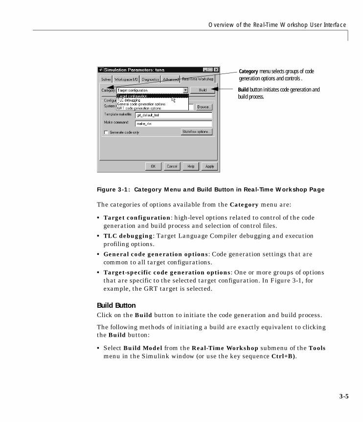
Overview of the Real-Time Workshop User Interface
3-5
Figure 3-1: Category Menu and Build Button in Real-Time Workshop Page
The categories of options available from the Category menu are:
• Target configuration: high-level options related to control of the codegeneration and build process and selection of control files.
• TLC debugging: Target Language Compiler debugging and executionprofiling options.
• General code generation options: Code generation settings that arecommon to all target configurations.
• Target-specific code generation options: One or more groups of optionsthat are specific to the selected target configuration. In Figure 3-1, forexample, the GRT target is selected.
Build ButtonClick on the Build button to initiate the code generation and build process.
The following methods of initiating a build are exactly equivalent to clickingthe Build button:
• Select Build Model from the Real-Time Workshop submenu of the Toolsmenu in the Simulink window (or use the key sequence Ctrl+B).
Category menu selects groups of code generation options and controls .
Build button initiates code generation and build process.
3 Code Generation and the Build Process
3-6
• Invoke the rtwbuild command from the MATLAB command line. The syntaxof the rtwbuild command isrtwbuild modelname
orrtwbuild('modelname')
where modelname is the name of the source model. If the source model is notloaded into Simulink, rtwbuild loads the model.
Using ToolTipsThe Real-Time Workshop page supports “ToolTip” online help. Place yourmouse over any edit field name or check box to display a message box thatexplains the option.
The following sections summarize each category of options or parameterscontrolled by the Real-Time Workshop page, with references to subsequentsections that give details on each option or parameter.

Overview of the Real-Time Workshop User Interface
3-7
Target Configuration OptionsFigure 3-2 shows the Target configuration options of the Real-TimeWorkshop page.
Figure 3-2: The Real-Time Workshop Page: Target Configuration Options
Browse ButtonThe Browse button opens the System Target File Browser (See Figure 3-6 onpage 3-35). The browser lets you select a preset target configuration consistingof a system target file, template makefile, and make command.
“Selecting a Target Configuration” on page 3-34 details the use of the browserand includes a complete list of available target configurations.
System Target File FieldThe System target file field has these functions:
Name of your model
Browse button opens System Target File Browser for selection of a target configuration.
System target file name is displayed or entered here.Specify TLC options afterfilename.
Make command name isdisplayed or entered here.Specify make options after make command name.
Target configuration category shows current configuration of system target file, template makefile, and make command for your desired target.
3 Code Generation and the Build Process
3-8
• If you have selected a target configuration using the System Target FileBrowser, this field displays the name of the chosen system target file(target.tlc).
• If you are using a target configuration that does not appear in the SystemTarget File Browser, you must enter the name of the desired system targetfile in this field.
• After the system target filename, you can enter code generation options andvariables for the Target Language Compiler. See “Target LanguageCompiler Variables and Options” on page 3-93 for details.
Template Makefile FieldThe Template makefile field has these functions:
• If you have selected a target configuration using the System Target FileBrowser, this field displays the name of the chosen template makefile.
• You can enter the name of the desired template makefile in this field. Youmust do this if you are using a target configuration that does not appear inthe System Target File Browser. This is necessary if you have written yourown template makefile for a custom target environment.
Make Command Field A high-level M-file command, invoked when a build is initiated, controls theReal-Time Workshop build process. Each target has an associated makecommand. The Make command field displays this command.
Almost all targets use the default command, make_rtw. “Targets Available fromthe System Target File Browser” on page 3-36 lists the make commandassociated with each target.
Third-party targets may supply another make command. See the vendor’sdocumentation.
In addition to the name of the make command, you can supply arguments in theMake command field. These arguments include compiler-specific options,include paths, and other parameters. When the build process invokes the makeutility, these arguments are passed along in the make command line.
“Template Makefiles and Make Options” on page 3-102 documents the Makecommand arguments you can use with each supported compiler.
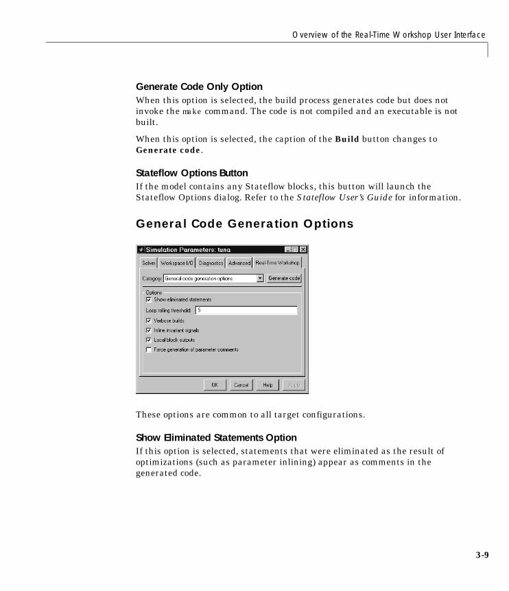
Overview of the Real-Time Workshop User Interface
3-9
Generate Code Only OptionWhen this option is selected, the build process generates code but does notinvoke the make command. The code is not compiled and an executable is notbuilt.
When this option is selected, the caption of the Build button changes toGenerate code.
Stateflow Options ButtonIf the model contains any Stateflow blocks, this button will launch theStateflow Options dialog. Refer to the Stateflow User’s Guide for information.
General Code Generation Options
These options are common to all target configurations.
Show Eliminated Statements OptionIf this option is selected, statements that were eliminated as the result ofoptimizations (such as parameter inlining) appear as comments in thegenerated code.

3 Code Generation and the Build Process
3-10
Loop Rolling Threshold FieldThe loop rolling threshold determines when a wide signal or parameter shouldbe wrapped into a for loop and when it should be generated as a separatestatement for each element of the signal. The default threshold value is 5.
For example, consider the model below
The gain parameter of the Gain block is the vector myGainVec.
Assume that the loop rolling threshold value is set to the default, 5.
If myGainVec is declared as
myGainVec = [1:10];
an array of 10 elements, rtP.Gain_Gain[] is declared within the Parametersdata structure, rtP. The size of the gain array exceeds the loop rollingthreshold. Therefore the code generated for the Gain block iterates over thearray in a for loop, as shown in the following code fragment.
/* Gain Block: <Root>/Gain */{int_T i1;
real_T *y0 = &rtB.Gain[0];const real_T *p_Gain_Gain = &rtP.Gain_Gain[0];

Overview of the Real-Time Workshop User Interface
3-11
for (i1=0; i1 < 10; i1++) {y0[i1] = rtb_foo * (p_Gain_Gain[i1]);}
}
If myGainVec is declared as
myGainVec = [1:3];
an array of 3 elements, rtP.Gain_Gain[] is declared within the Parametersdata structure, rtP. The size of the gain array is below the loop rollingthreshold. The generated code consists of inline references to each element ofthe array, as in the code fragment below.
/* Gain Block: <Root>/Gain */rtB.Gain[0] = rtb_foo * (rtP.Gain_Gain[0]);rtB.Gain[1] = rtb_foo * (rtP.Gain_Gain[1]);rtB.Gain[2] = rtb_foo * (rtP.Gain_Gain[2]);
See the Target Language Compiler Reference Guide for more information onloop rolling.
Verbose Builds OptionIf this option is selected, the MATLAB command window displays progressinformation during code generation; compiler output is also made visible.
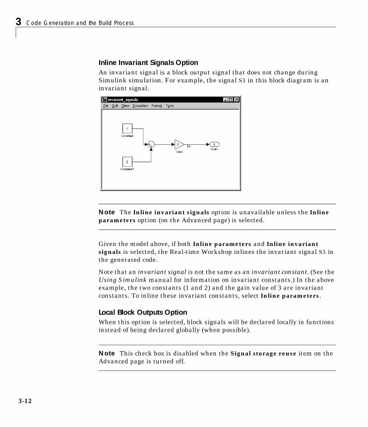
3 Code Generation and the Build Process
3-12
Inline Invariant Signals OptionAn invariant signal is a block output signal that does not change duringSimulink simulation. For example, the signal S3 in this block diagram is aninvariant signal.
Note The Inline invariant signals option is unavailable unless the Inlineparameters option (on the Advanced page) is selected.
Given the model above, if both Inline parameters and Inline invariantsignals is selected, the Real-time Workshop inlines the invariant signal S3 inthe generated code.
Note that an invariant signal is not the same as an invariant constant. (See theUsing Simulink manual for information on invariant constants.) In the aboveexample, the two constants (1 and 2) and the gain value of 3 are invariantconstants. To inline these invariant constants, select Inline parameters.
Local Block Outputs OptionWhen this option is selected, block signals will be declared locally in functionsinstead of being declared globally (when possible).
Note This check box is disabled when the Signal storage reuse item on theAdvanced page is turned off.
Overview of the Real-Time Workshop User Interface
3-13
For further information on the use of the Local block outputs option, see:
• “Signals: Storage, Optimization, and Interfacing” on page 3-65
• “Tutorial 4: A First Look at Generated Code” on page 1–56
Force Generation of Parameter Comments OptionThe Force generation of parameter comments option controls the generationof comments in the model parameter structure declaration in model_prm.h.Parameter comments indicate parameter variable names and the names ofsource blocks.
When this option is off (the default), parameter comments are generated if lessthan 1000 parameters are declared. This reduces the size of the generated filefor models with a large number of parameters.
When this option is on, parameter comments are generated regardless of thenumber of parameters.
Target Specific Code Generation OptionsDifferent target configurations support different code generation options thatare not supported by all available targets. For example, the grt, grt_malloc,Tornado, xPC, and Real-Time Windows targets support external mode, butother targets do not.
This section summarizes the options specific to the generic real-time (GRT)target. For information on options specific to other targets, see thedocumentation relevant to those targets. “Available Targets” on page 3-36 liststargets and related chapters and manuals.
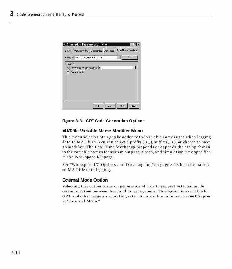
3 Code Generation and the Build Process
3-14
Figure 3-3: GRT Code Generation Options
MAT-file Variable Name Modifier MenuThis menu selects a string to be added to the variable names used when loggingdata to MAT-files. You can select a prefix (rt_), suffix (_rt), or choose to haveno modifier. The Real-Time Workshop prepends or appends the string chosento the variable names for system outputs, states, and simulation time specifiedin the Workspace I/O page.
See “Workspace I/O Options and Data Logging” on page 3-18 for informationon MAT-file data logging.
External Mode OptionSelecting this option turns on generation of code to support external modecommunication between host and target systems. This option is available forGRT and other targets supporting external mode. For information see Chapter5, “External Mode.”
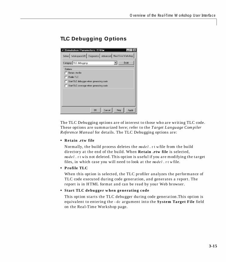
Overview of the Real-Time Workshop User Interface
3-15
TLC Debugging Options
The TLC Debugging options are of interest to those who are writing TLC code.These options are summarized here; refer to the Target Language CompilerReference Manual for details. The TLC Debugging options are:
• Retain .rtw file
Normally, the build process deletes the model.rtw file from the builddirectory at the end of the build. When Retain .rtw file is selected,model.rtw is not deleted. This option is useful if you are modifying the targetfiles, in which case you will need to look at the model.rtw file.
• Profile TLC
When this option is selected, the TLC profiler analyzes the performance ofTLC code executed during code generation, and generates a report. Thereport is in HTML format and can be read by your Web browser.
• Start TLC debugger when generating code
This option starts the TLC debugger during code generation.This option isequivalent to entering the -dc argument into the System Target File fieldon the Real-Time Workshop page.
3 Code Generation and the Build Process
3-16
• Start TLC coverage when generating code
When this option is selected, the Target Language Compiler generates areport containing statistics indicating how many times each line of TLC codeis hit during code generation.
This option is equivalent to entering the -dg argument into the SystemTarget File field on the Real-Time Workshop page.
Real-Time Workshop Submenu• The Tools menu of the Simulink window contains a Real-Time Workshop
submenu. The submenu items are:
- Options: Open the Real-Time Workshop page of the SimulationParameters dialog.
- Build Model: Initiate code generation and build process; equivalent toclicking the Build button in the Real-Time Workshop page.
- Build Subsystem: Generate code and build an executable from asubsystem; enabled only when a subsystem is selected. See “GeneratingCode and Executables from Subsystems” on page 3-49.
- Generate S-Function: Generate code and build an S-function from asubsystem; enabled only when a subsystem is selected. See “AutomatedS-Function Generation” on page 10-12.
Simulation Parameters and Code Generation
3-17
Simulation Parameters and Code GenerationThis section discusses how the simulation parameters of your model interactwith Real-Time Workshop code generation. Only simulation parameters thataffect code generation are mentioned here. For a full description of simulationparameters, see the Using Simulink manual.
This discussion is organized around the following pages of the SimulationParameters dialog box:
• Solver page
• Workspace I/O page
• Diagnostics page
• Advanced Page
To view these pages, choose Simulation parameters from the Simulationmenu. When the dialog box opens, click the appropriate tab.
Solver Options
Solver Type. If you are using the S-Function Target, you can specify either afixed-step or a variable-step solver. All other targets require a fixed-step solver.
Mode. Real-Time Workshop supports both single- and multitasking modes. SeeChapter 7, “Models with Multiple Sample Rates” for full details.
Start and Stop Times. The stop time must be greater than or equal to the starttime. If the stop time is zero, or if the total simulation time (Stop - Start) isless than zero, the generated program runs for one step. If the stop time is setto inf, the generated program runs indefinitely.
Note that when using the GRT or Tornado targets, you can override the stoptime when running a generated program from the DOS or UNIX command line.To override the stop time that was set during code generation, use the -tfswitch.
modelname -tf n
The program will run for n seconds. If n = inf, the program will runindefinitely. See “Part 3: Running the External Mode Target Program” on page5-11 for an example of the use of this option.
3 Code Generation and the Build Process
3-18
Note Certain blocks have a dependency on absolute time. If you aredesigning a program that is intended to run indefinitely (Stop time = inf), youmust not use these blocks. See Appendix A for a list of blocks that depend onabsolute time.
Workspace I/O Options and Data LoggingThis section discusses several different methods by which a Real-TimeWorkshop generated program can save data to a MAT-file for later analysis.These methods include:
• Using the Workspace I/O page to define and log workspace return variables
• Logging data from Scope and To Workspace blocks
• Logging data using To File blocks
“Tutorial 2: Data Logging” on page 1-49 is an exercise designed to give youhands-on experience with data logging features of the Real-Time Workshop.
Note Data logging is available only for targets that have access to a filesystem.
Logging States, Time, and Outputs via the Workspace I/O PageThe Workspace I/O page enables a generated program to save system states,outputs, and simulation time at each model execution time step. The data iswritten to a MAT-file, named (by default) model.mat.
Before using this data logging feature, you should learn how to configure aSimulink model to return output to the MATLAB workspace. This is discussedin the Using Simulink manual.
For each workspace return variable that you define and enable, Real-TimeWorkshop defines a MAT-file variable. For example, if your model savessimulation time to the workspace variable tout, your generated program willlog the same data to a variable named (by default) rt_tout.
Simulation Parameters and Code Generation
3-19
The Real-Time Workshop logs the following data:
• All root Outport blocks
The default MAT-file variable name for system outputs is rt_yout.
The sort order of the rt_yout array is based on the port number of theOutport block, starting with 1.
• All continuous and discrete states in the model
The default MAT-file variable name for system states is rt_xout.
• Simulation time
The default MAT-file variable name for simulation time is rt_tout.
Real-Time Workshop data logging follows the Workspace I/O Save options:(Limit data points, Decimation, and Format).
Overriding the Default MAT-File Name. The MAT-file name defaults to model.mat.To specify a different filename:
1 Choose Simulation parameters from the Simulation menu. The dialog boxopens. Click the Real-Time Workshop tab.
2 Append the following option to the existing text in the Make command field.
OPTS="-DSAVEFILE=filename"
Overriding Default MAT-File Variable Names. By default, the Real-Time Workshopprepends the string rt_ to the variable names for system outputs, states, andsimulation time to form MAT-file variable names. To change this prefix:
1 Choose Simulation parameters from the Simulation menu. The dialog boxopens. Click the Real-Time Workshop tab.
2 Select the target-specific code generation options item from the Categorymenu.
3 Select a prefix(rt_) or suffix (_rt) from the MAT-file variable namemodifier field, or choose none for no prefix.
3 Code Generation and the Build Process
3-20
Logging Data with Scope and To Workspace BlocksThe Real-Time Workshop also logs data from these sources:
• All Scope blocks that have the save data to workspace option enabled
You must specify the variable name and data format in each Scope block’sdialog box.
• All To Workspace blocks in the model
You must specify the variable name and data format in each To Workspaceblock’s dialog box.
The variables are written to model.mat, along with any variables logged fromthe Workspace I/O page.
Logging Data with To File Blocks
You can also log data to a To File block. The generated program creates aseparate MAT-file (distinct from model.mat) for each To File block in the model.The file contains the block’s time and input variable(s). You must specify thefilename, variable name(s), decimation, and sample time in the To File block’sdialog box.
Note that the To File block cannot be used in DOS real-time targets because oflimitations of the DOS target.
Data Logging Differences in Single- and Multitasking ModelsWhen logging data in singletasking and multitasking systems, you will noticedifferences in the logging of:
• Noncontinuous root Outport blocks
• Discrete states
In multitasking mode, the logging of states and outputs is done after the firsttask execution (and not at the end of the first time step). In singletasking mode,the Real-Time Workshop logs states and outputs after the first time step.
See “Data Logging In Single- and Multitasking Model Execution” on page 6–14for more details on the differences between single- and multitasking datalogging.

Simulation Parameters and Code Generation
3-21
Note The rapid simulation target (rsim) provides enhanced logging options.See Chapter 11, “Real-Time Workshop Rapid Simulation Target” for moreinformation.
Diagnostics Page Options
The Diagnostics page specifies what action should be taken when variousmodel conditions such as unconnected ports are encountered. You can specifywhether to ignore a given condition, issue a warning, or raise an error. If anerror condition is encountered during a build, the build is terminated. TheDiagnostics page is fully documented in the Using Simulink manual.
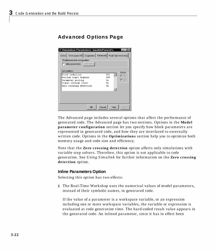
3 Code Generation and the Build Process
3-22
Advanced Options Page
The Advanced page includes several options that affect the performance ofgenerated code. The Advanced page has two sections. Options in the Modelparameter configuration section let you specify how block parameters arerepresented in generated code, and how they are interfaced to externallywritten code. Options in the Optimizations section help you to optimize bothmemory usage and code size and efficiency.
Note that the Zero crossing detection option affects only simulations withvariable step solvers. Therefore, this option is not applicable to codegeneration. See Using Simulink for further information on the Zero crossingdetection option.
Inline Parameters OptionSelecting this option has two effects:
1 The Real-Time Workshop uses the numerical values of model parameters,instead of their symbolic names, in generated code.
If the value of a parameter is a workspace variable, or an expressionincluding one or more workspace variables, the variable or expression isevaluated at code generation time. The hard-coded result value appears inthe generated code. An inlined parameter, since it has in effect been

Simulation Parameters and Code Generation
3-23
transformed into a constant, is no longer tunable. That is, it is not visible toexternally-written code, and its value cannot be changed at run-time.
2 The Configure button becomes enabled. Clicking the Configure buttonopens the Model Parameter Configuration dialog.
The Model Parameter Configuration dialog lets you remove individualparameters from inlining and declare them to be tunable variables (or globalconstants). When you declare a parameter tunable, the Real-Time Workshopgenerates a storage declaration that allows the parameter to be interfacedto externally-written code. This enables your hand-written code to changethe value of the parameter at run-time.
The Model Parameter Configuration dialog lets you improve overallefficiency by inlining most parameters, while at the same time retaining theflexibility of run-time tuning for selected parameters.
See “Parameters: Storage, Interfacing, and Tuning” on page 3-51 for furtherinformation on interfacing parameters to externally-written code.
Inline parameters also instructs Simulink to propagate constant sampletimes. Simulink computes the output signals of blocks that have constantsample times once during model startup. This improves performance, sincesuch blocks do not compute their outputs at every time step of the model.
Selecting Inline parameters also interacts with other code generationparameters as follows:
• When Inline parameters is selected, the Inline invariant signals codegeneration option becomes available. See “Inline Invariant Signals Option”on page 3-12.
• You cannot inline parameters when using external mode. External moderequires that all parameters be tunable. See Chapter 5, “External Mode.”
• The Parameter pooling option is used only when Inline parameters isselected. See “Parameter Pooling Option” on page 3-24.
Block Reduction OptionWhen this option is selected, Simulink collapses certain groups of blocks into asingle, more efficient block, or removes them entirely. This results in fastermodel execution during simulation and in generated code. The appearance of

3 Code Generation and the Build Process
3-24
the source model does not change. The types of block reduction optimizationscurrently supported are:
• Accumulator folding: Simulink recognizes certain constructs asaccumulators, and reduces them to a single block. For a detailed example,see “Accumulators” on page 8-15.
• Unnecessary type conversion blocks are removed. For example, an int typeconversion block whose input and output are of type int is redundant andwill be removed.
Boolean Logic Signals OptionBy default, Simulink does not signal an error when it detects that doublesignals are connected to blocks that prefer Boolean input. This ensurescompatibility with models created by earlier versions of Simulink that supportonly double data type. You can enable strict Boolean type checking by selectingthe Boolean logic signals option.
Selecting this option is recommended. Generated code will require lessmemory, because a Boolean signal typically requires one byte of storage whilea double signal requires eight bytes of storage.
Parameter Pooling OptionParameter pooling occurs when multiple block parameters refer to storagelocations that are separately defined but structurally identical. Theoptimization is similar to that of a C compiler that encounters declarationssuch as
int a[] = {1,2,3}; int b[] = {1,2,3};
In such a case, an optimizing compiler would collapse a and b into a single textlocation containing the values 1,2,3 and initialize a and b from the same code.
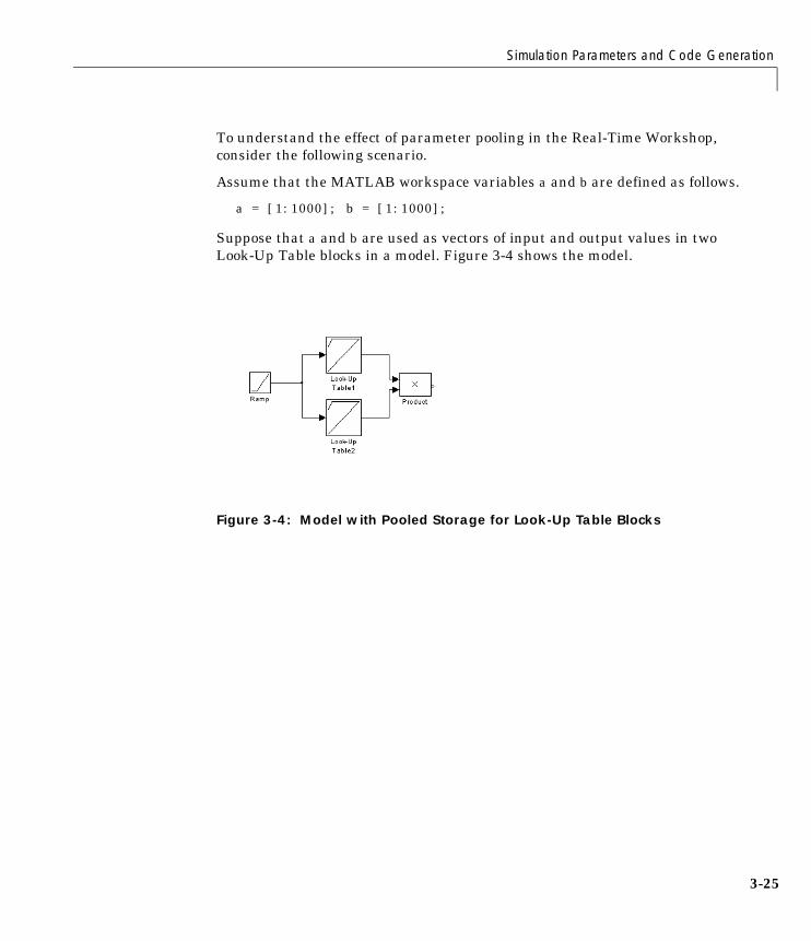
Simulation Parameters and Code Generation
3-25
To understand the effect of parameter pooling in the Real-Time Workshop,consider the following scenario.
Assume that the MATLAB workspace variables a and b are defined as follows.
a = [1:1000]; b = [1:1000];
Suppose that a and b are used as vectors of input and output values in twoLook-Up Table blocks in a model. Figure 3-4 shows the model.
Figure 3-4: Model with Pooled Storage for Look-Up Table Blocks

3 Code Generation and the Build Process
3-26
Figure 3-5 shows the use of a and b as a parameters of Look-Up Table1andLook-Up Table2.
Figure 3-5: Pooled Storage in Look-Up Table Blocks
If Parameter pooling is on, pooled storage is used for the input/output data ofthe Look-Up Table blocks. The following code fragment shows the definition ofthe global parameter structure of the model (rtP). The input data referencesto a and b are pooled in the field rtP.p2. Likewise, while the output datareferences (expressions including a and b) are pooled in the field rtP.p3.
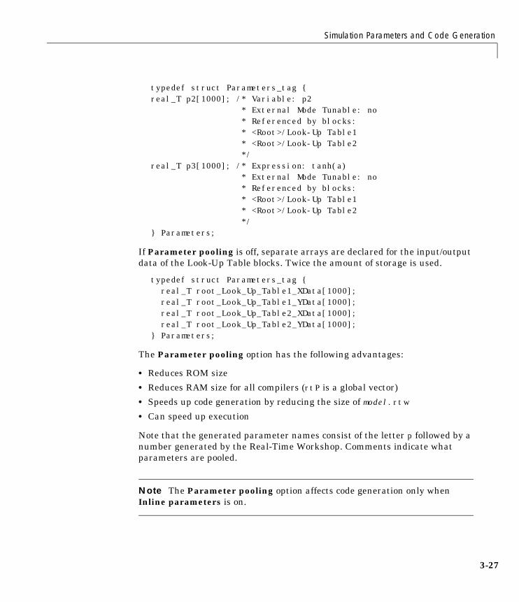
Simulation Parameters and Code Generation
3-27
typedef struct Parameters_tag {real_T p2[1000]; /* Variable: p2
* External Mode Tunable: no* Referenced by blocks:* <Root>/Look-Up Table1* <Root>/Look-Up Table2*/
real_T p3[1000]; /* Expression: tanh(a)* External Mode Tunable: no* Referenced by blocks:* <Root>/Look-Up Table1* <Root>/Look-Up Table2*/
} Parameters;
If Parameter pooling is off, separate arrays are declared for the input/outputdata of the Look-Up Table blocks. Twice the amount of storage is used.
typedef struct Parameters_tag {real_T root_Look_Up_Table1_XData[1000]; real_T root_Look_Up_Table1_YData[1000];real_T root_Look_Up_Table2_XData[1000];real_T root_Look_Up_Table2_YData[1000];
} Parameters;
The Parameter pooling option has the following advantages:
• Reduces ROM size
• Reduces RAM size for all compilers (rtP is a global vector)
• Speeds up code generation by reducing the size of model.rtw
• Can speed up execution
Note that the generated parameter names consist of the letter p followed by anumber generated by the Real-Time Workshop. Comments indicate whatparameters are pooled.
Note The Parameter pooling option affects code generation only whenInline parameters is on.
3 Code Generation and the Build Process
3-28
Signal Storage Reuse OptionThis option instructs the Real-Time Workshop to reuse signal memory. Thisreduces the memory requirements of your real-time program. Selecting thisoption is recommended. Disabling Signal storage reuse makes all blockoutputs global and unique, which in many cases significantly increases RAMand ROM usage.
For further details on the Signal storage reuse option, see “Signals: Storage,Optimization, and Interfacing” on page 3-65.
Note Selecting Signal storage reuse also enables the Local block outputsoption in the General code generation options category of the Real-TimeWorkshop page. See “Local Block Outputs Option” on page 3-12.
Tracing Generated Code Back to Your Simulink ModelThe Real-Time Workshop writes system/block identification tags in thegenerated code. The tags are designed to help you identify the block, in yoursource model, that generated a given line of code. Tags are located in commentlines above each line of generated code.
The tag format is <system>/block_name, where:
• system is either:
- the string 'root', or
- a unique system number assigned by Simulink
• block_name is the name of the block.
The following code fragment illustrates a tag comment adjacent to a line of codegenerated by a Gain block at the root level of the source model.
/* Gain Block: <Root>/Gain */rtb_temp3 *= (rtP.root_Gain_Gain);
The following code fragment illustrates a tag comment adjacent to a line of codegenerated by a Gain block within a subsystem one level below the root level ofthe source model.
Simulation Parameters and Code Generation
3-29
/* Gain Block: <S1>/Gain */rtB.temp0 *= (rtP.s1_Gain_Gain);
In addition to the tags, the Real-Time Workshop documents the tags for eachmodel in comments in the generated header file model.h. The followingillustrates such a comment, generated from a source model, foo. foo has asubsystem Outer with a nested subsystem Inner.
/* Here is the system hierarchy for this model. * * <Root> : foo * <S1> : foo/Outer * <S2> : foo/Outer/Inner */
To trace a tag back to the generating block:
1 Open the source model.
2 Close any other model windows that are open.
3 Use the MATLAB hilite_system command to view the desired system andblock.
As an example, consider the model foo mentioned above. If foo is open,
hilite_system('<S1>')
opens the subsystem Outer and
hilite_system('<S2>/Gain1')
opens the subsystem Outer and selects and highlights the Gain block Gain1within that subsystem.
Other Interactions Between Simulink and the Real-Time WorkshopThe Simulink engine propagates data from one block to the next along signallines. The data propagated are:
• Data type
• Line widths

3 Code Generation and the Build Process
3-30
• Sample times
The first stage of code generation is compilation of the block diagram. Thiscompile stage is analogous to that of a C program. The C compiler carries outtype checking and pre-processing. Similarly, Simulink verifies that input/output data types of block ports are consistent, line widths between blocks areof the correct thickness, and the sample times of connecting blocks areconsistent.
The Simulink engine typically derives signal attributes from a source block.For example, the Inport block’s parameters dialog box specifies the signalattributes for the block.
In this example, the Inport block has a port width of 3, a sample time of .01seconds, the data type is double, and the signal is complex.
This figure shows the propagation of the signal attributes associated with theInport block through a simple block diagram.
In this example, the Gain and Outport blocks inherit the attributes specifiedfor the Inport block.
Simulation Parameters and Code Generation
3-31
Sample Time PropagationInherited sample times in source blocks (e.g., a root inport) can sometimes leadto unexpected and unintended sample time assignments. Since a block mayspecify an inherited sample time, information available at the outset is ofteninsufficient to compile a block diagram completely. In such cases, the Simulinkengine propagates the known or assigned sample times to those blocks thathave inherited sample times but which have not yet been assigned a sampletime. Thus, Simulink continues to fill in the blanks (the unknown sampletimes) until sample times have been assigned to as many blocks as possible.Blocks that still do not have a sample time are assigned a default sample timeaccording to the following rules:
1 If the current system has at least one rate in it, the block is assigned thefastest rate.
2 If no rate exists and the model is configured for a variable-step solver, theblock is assigned a continuous sample time (but fixed in minor time steps).Note that the Real-Time Workshop (with the exception of the S-FunctionTarget) does not currently support variable-step solvers.
3 If no rate exists and the model is configured for a fixed-step solver, the blockis assigned a discrete sample time of (Tf - Ti)/50, where Ti is the simulationstart time and Tf is the simulation stop time. If Tf is infinity, the defaultsample time is set to 0.2.
To ensure a completely deterministic model (one where no sample times are setusing the above rules), you should explicitly specify the sample time of all yoursource blocks. Source blocks include root inport blocks and any blocks withoutinput ports. You do not have to set subsystem input port sample times. Youmay want to do so, however, when creating modular systems.

3 Code Generation and the Build Process
3-32
An unconnected input implicitly sources ground. For ground blocks and groundconnections, the default sample time is derived from destination blocks or thedefault rule.
Block Execution OrderOnce Simulink compiles the block diagram, it creates a model.rtw file(analogous to an object file generated from a C file). The model.rtw filecontains all the connection information of the model, as well as the necessarysignal attributes. Thus, the timing engine in the Real-Time Workshop knowswhen blocks with different rates should be executed.
You cannot override this execution order by directly calling a block (inhand-written code) in a model. For example, the disconnected_trigger modelbelow will have its trigger port source to ground, which may lead to all blocksinheriting a constant sample time. Calling the trigger function, f(), directlyfrom hand-code will not work correctly and should never be done. Instead, youshould use a function-call generator to properly specify the rate at which f()should be executed, as shown in the connected_trigger model below.
All blocks have an inheritedsample time (Ts = -1). They willall be assigned a sample time of(Tf - Ti)/50.

Simulation Parameters and Code Generation
3-33
Instead of the function-call generator, you could use any other block that candrive the trigger port. Then, you should call the model’s main entry point toexecute the trigger function.
For multirate models, a common use of the Real-Time Workshop is to buildindividual models separately and then hand-code the I/O between the models.This approach places the burden of data consistency between models on thedeveloper of the models. Another approach is to let Simulink and theReal-Time Workshop ensure data consistency between rates and generatemultirate code for use in a multitasking environment. The Real-TimeWorkshop Interrupt Template and VxWorks Support libraries provide blockswhich allow synchronous and asynchronous data flow. For a description of theReal-Time Workshop libraries, see Chapter 14, “Custom Code Blocks” andChapter 15, “Asynchronous Support.” For more information on multi-rate codegeneration, see Chapter 7, “Models with Multiple Sample Rates.”
3 Code Generation and the Build Process
3-34
Selecting a Target ConfigurationThe process of generating target-specific code is controlled by a configurationof:
• A system target file
• A template makefile
• A make command
The System Target File Browser lets you specify such a configuration in asingle step, choosing from a wide variety of ready-to-run configurations.
The System Target File BrowserTo select a target configuration using the System Target File Browser:
1 Click the Real-Time Workshop tab of the Simulation Parameters dialogbox. The Real-Time Workshop page activates.
2 Select Target configuration from the Category menu.
3 Click the Browse button next to the System target file field. This opens theSystem Target File Browser. The browser displays a list of all currentlyavailable target configurations. When you select a target configuration, theReal-Time Workshop automatically chooses the appropriate system targetfile, template makefile, and make command.
Figure 3-6 shows the System Target File Browser with the generic real-timetarget selected.
4 Double-click on the desired entry in the list of available configurations.Alternatively, you can select the desired entry in the list and click OK.
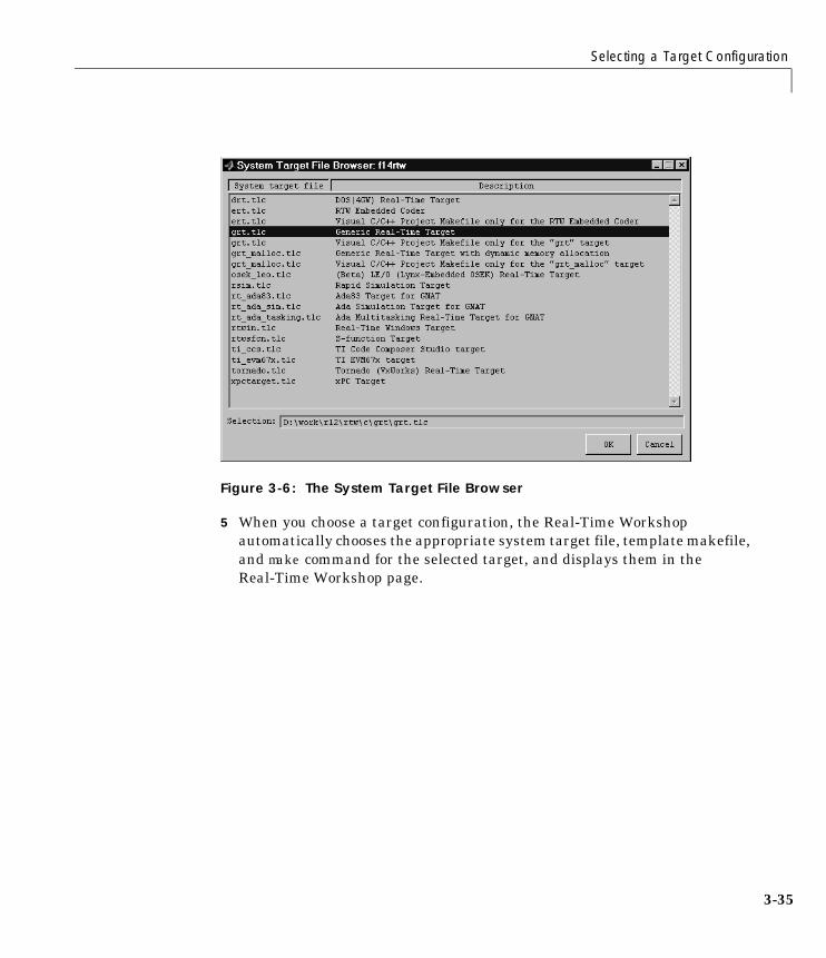
Selecting a Target Configuration
3-35
Figure 3-6: The System Target File Browser
5 When you choose a target configuration, the Real-Time Workshopautomatically chooses the appropriate system target file, template makefile,and make command for the selected target, and displays them in theReal-Time Workshop page.
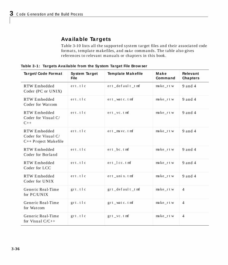
3 Code Generation and the Build Process
3-36
Available TargetsTable 3-10 lists all the supported system target files and their associated codeformats, template makefiles, and make commands. The table also givesreferences to relevant manuals or chapters in this book.
Table 3-1: Targets Available from the System Target File Browser
Target/Code Format System Target File
Template Makefile Make Command
Relevant Chapters
RTW EmbeddedCoder (PC or UNIX)
ert.tlc ert_default_tmf make_rtw 9 and 4
RTW EmbeddedCoder for Watcom
ert.tlc ert_watc.tmf make_rtw 9 and 4
RTW EmbeddedCoder for Visual C/C++
ert.tlc ert_vc.tmf make_rtw 9 and 4
RTW EmbeddedCoder for Visual C/C++ Project Makefile
ert.tlc ert_msvc.tmf make_rtw 9 and 4
RTW EmbeddedCoder for Borland
ert.tlc ert_bc.tmf make_rtw 9 and 4
RTW EmbeddedCoder for LCC
ert.tlc ert_lcc.tmf make_rtw 9 and 4
RTW EmbeddedCoder for UNIX
ert.tlc ert_unix.tmf make_rtw 9 and 4
Generic Real-Timefor PC/UNIX
grt.tlc grt_default_tmf make_rtw 4
Generic Real-Timefor Watcom
grt.tlc grt_watc.tmf make_rtw 4
Generic Real-Timefor Visual C/C++
grt.tlc grt_vc.tmf make_rtw 4
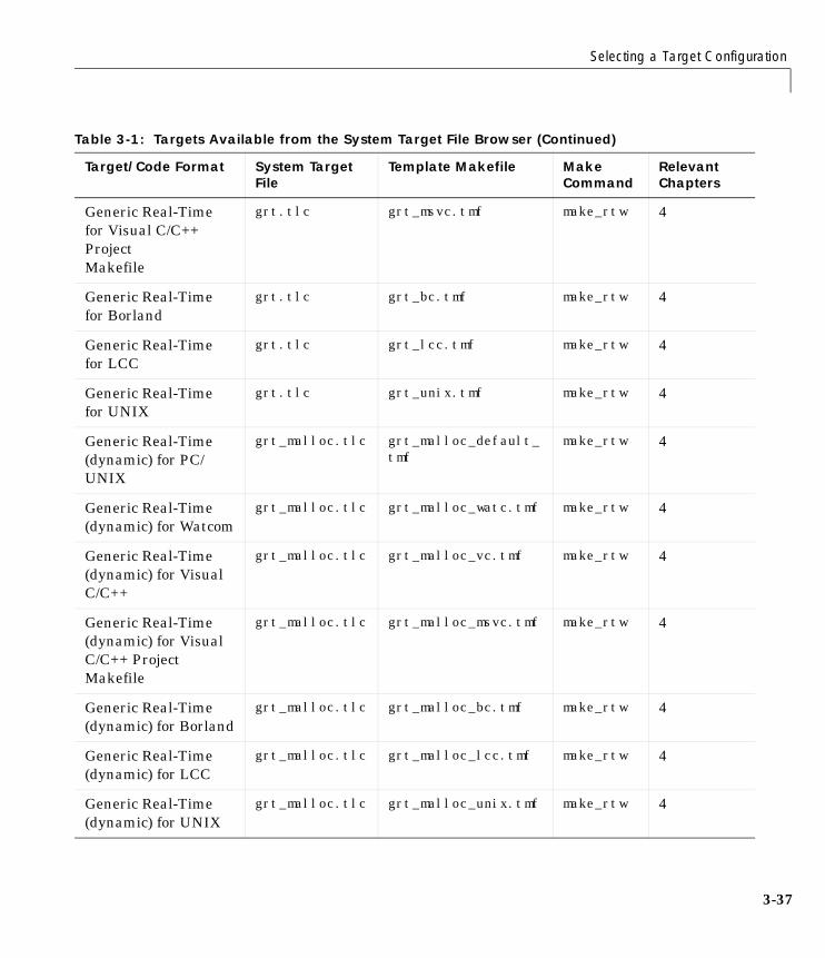
Selecting a Target Configuration
3-37
Generic Real-Timefor Visual C/C++ProjectMakefile
grt.tlc grt_msvc.tmf make_rtw 4
Generic Real-Timefor Borland
grt.tlc grt_bc.tmf make_rtw 4
Generic Real-Timefor LCC
grt.tlc grt_lcc.tmf make_rtw 4
Generic Real-Timefor UNIX
grt.tlc grt_unix.tmf make_rtw 4
Generic Real-Time(dynamic) for PC/UNIX
grt_malloc.tlc grt_malloc_default_tmf
make_rtw 4
Generic Real-Time(dynamic) for Watcom
grt_malloc.tlc grt_malloc_watc.tmf make_rtw 4
Generic Real-Time(dynamic) for VisualC/C++
grt_malloc.tlc grt_malloc_vc.tmf make_rtw 4
Generic Real-Time(dynamic) for VisualC/C++ ProjectMakefile
grt_malloc.tlc grt_malloc_msvc.tmf make_rtw 4
Generic Real-Time(dynamic) for Borland
grt_malloc.tlc grt_malloc_bc.tmf make_rtw 4
Generic Real-Time(dynamic) for LCC
grt_malloc.tlc grt_malloc_lcc.tmf make_rtw 4
Generic Real-Time(dynamic) for UNIX
grt_malloc.tlc grt_malloc_unix.tmf make_rtw 4
Table 3-1: Targets Available from the System Target File Browser (Continued)
Target/Code Format System Target File
Template Makefile Make Command
Relevant Chapters
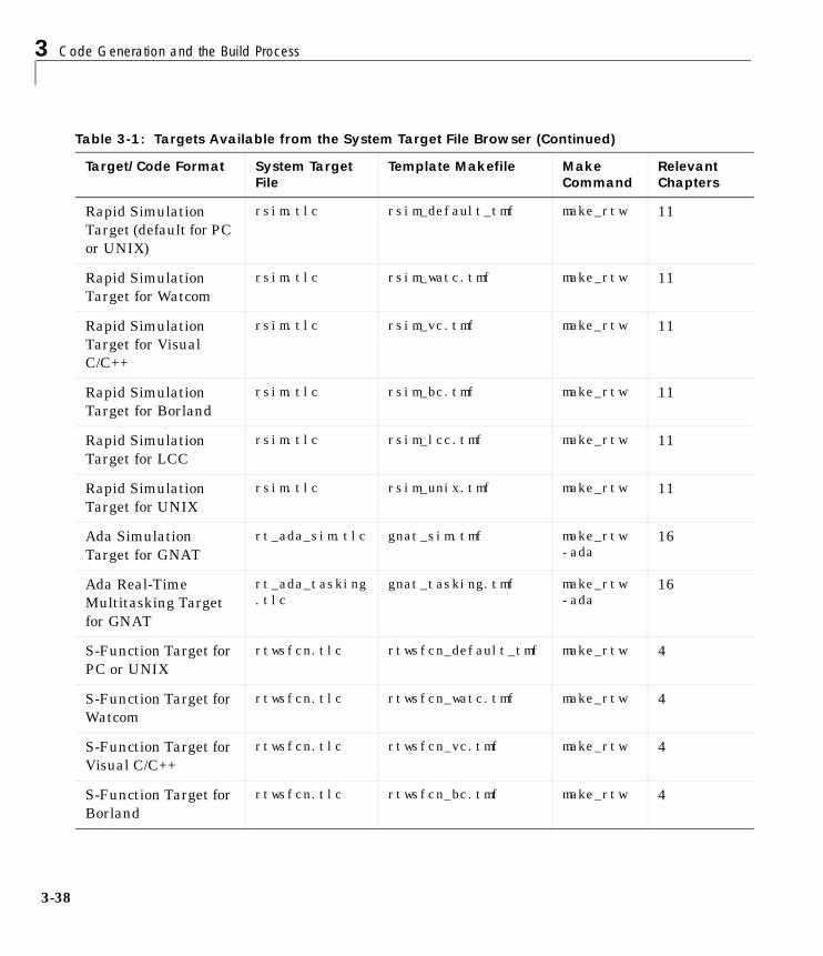
3 Code Generation and the Build Process
3-38
Rapid SimulationTarget (default for PCor UNIX)
rsim.tlc rsim_default_tmf make_rtw 11
Rapid SimulationTarget for Watcom
rsim.tlc rsim_watc.tmf make_rtw 11
Rapid SimulationTarget for VisualC/C++
rsim.tlc rsim_vc.tmf make_rtw 11
Rapid SimulationTarget for Borland
rsim.tlc rsim_bc.tmf make_rtw 11
Rapid SimulationTarget for LCC
rsim.tlc rsim_lcc.tmf make_rtw 11
Rapid SimulationTarget for UNIX
rsim.tlc rsim_unix.tmf make_rtw 11
Ada SimulationTarget for GNAT
rt_ada_sim.tlc gnat_sim.tmf make_rtw -ada
16
Ada Real-TimeMultitasking Targetfor GNAT
rt_ada_tasking.tlc
gnat_tasking.tmf make_rtw -ada
16
S-Function Target forPC or UNIX
rtwsfcn.tlc rtwsfcn_default_tmf make_rtw 4
S-Function Target forWatcom
rtwsfcn.tlc rtwsfcn_watc.tmf make_rtw 4
S-Function Target forVisual C/C++
rtwsfcn.tlc rtwsfcn_vc.tmf make_rtw 4
S-Function Target forBorland
rtwsfcn.tlc rtwsfcn_bc.tmf make_rtw 4
Table 3-1: Targets Available from the System Target File Browser (Continued)
Target/Code Format System Target File
Template Makefile Make Command
Relevant Chapters
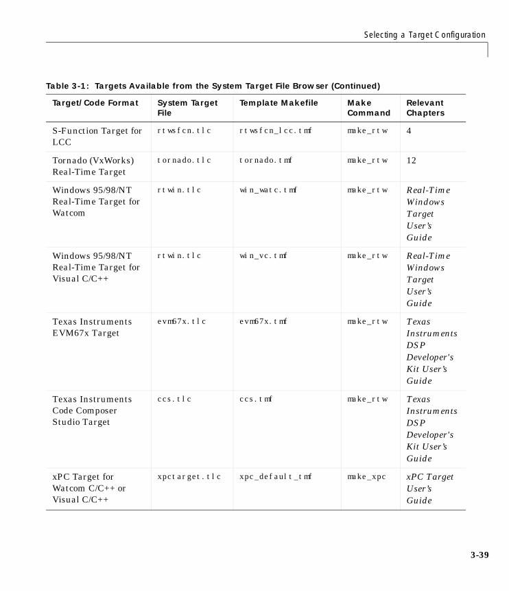
Selecting a Target Configuration
3-39
S-Function Target forLCC
rtwsfcn.tlc rtwsfcn_lcc.tmf make_rtw 4
Tornado (VxWorks)Real-Time Target
tornado.tlc tornado.tmf make_rtw 12
Windows 95/98/NTReal-Time Target forWatcom
rtwin.tlc win_watc.tmf make_rtw Real-TimeWindowsTargetUser’sGuide
Windows 95/98/NTReal-Time Target forVisual C/C++
rtwin.tlc win_vc.tmf make_rtw Real-TimeWindowsTargetUser’sGuide
Texas InstrumentsEVM67x Target
evm67x.tlc evm67x.tmf make_rtw TexasInstrumentsDSPDeveloper'sKit User’sGuide
Texas InstrumentsCode ComposerStudio Target
ccs.tlc ccs.tmf make_rtw TexasInstrumentsDSPDeveloper'sKit User’sGuide
xPC Target forWatcom C/C++ orVisual C/C++
xpctarget.tlc xpc_default_tmf make_xpc xPC TargetUser’sGuide
Table 3-1: Targets Available from the System Target File Browser (Continued)
Target/Code Format System Target File
Template Makefile Make Command
Relevant Chapters

3 Code Generation and the Build Process
3-40
Note The LE/O and DOS targets are included as examples only.
DOS (4GW) drt.tlc drt_watc.tmf make_rtw 13 and 4
LE/O (Lynxembedded OSEK)Real-Time Target
osek_leo.tlc osek_leo.tmf make_rtw MAT_FILE=1RUN=1 LEO_NODE=osek
Readme fileinmatlabroot/rtw/c/osek_leo
Table 3-1: Targets Available from the System Target File Browser (Continued)
Target/Code Format System Target File
Template Makefile Make Command
Relevant Chapters
Nonvirtual Subsystem Code Generation
3-41
Nonvirtual Subsystem Code GenerationThe Real-Time Workshop allows you to control generation of code at thesubsystem level, for any nonvirtual subsystem. The categories of nonvirtualsubsystems are:
• Conditionally executed subsystems: execution depends upon a control signal.These include triggered subsystems, enabled subsystems, subsystems thatare both triggered and enabled, and function call subsystems. See UsingSimulink for information on conditionally executed subsystems.
• Atomic subsystems: Any virtual subsystem can be declared atomic (andtherefore nonvirtual) via the Treat as atomic unit option in the BlockParameters dialog.
See Using Simulink for further information on virtual subsystems and atomicsubsystems.
You can control the code generated from nonvirtual subsystems as follows:
• You can instruct the Real-Time Workshop to generate separate functions,within separate code files, for selected nonvirtual systems. You can controlboth the names of the functions and of the code files generated fromnonvirtual subsystems.
• You can generate inlined code from selected nonvirtual subsystems withinyour model. When you inline a nonvirtual subsystem, a separate functioncall is not generated for the subsystem.
Nonvirtual Subsystem Code Generation OptionsFor any nonvirtual subsystem, you can choose the following code generationoptions from the RTW system code pop-up menu in the subsystem Blockparameters dialog:
• Auto: This is the default option. See “Auto Option” below.
• Inline: This option explicitly directs the Real-Time Workshop to inline thesubsystem.
• Function: This option explicitly directs the Real-Time Workshop to generatea separate function and file for the subsystem. In this case you can choosefurther options to control the naming of the generated function and file.
The sections below discuss the Auto, Inline, and Function options.
3 Code Generation and the Build Process
3-42
Auto OptionIn the current release, the Auto option causes the Real-Time Workshop toinline the subsystem, unless it is a function-call subsystem with multiplecallers. In that case, a function is generated.
In a future release, the Auto option will also create functions when multipleinstances of a subsystem are detected. If there are multiple instances ormultiple callers of the subsystem, the subsystem will not be inlined. To takeadvantage of this capability, you should choose the Auto option. Choose Inlineor Function when you want specifically to inline a subsystem or generate aseparate function and code module.
To use the Auto option:
1 Select the subsystem block. Then select Subsystem parameters from theSimulink Edit menu. The Block Parameters dialog opens, as shown inFigure 3-7.
Alternatively, you can open the Block Parameters dialog by:
- Shift-double-clicking on the Subsystem block
- Right-clicking on the Subsystem block and selecting Block parametersfrom the pop-up menu.
2 If the subsystem is virtual, select Treat as atomic unit as shown inFigure 3-7. This makes the subsystem nonvirtual, and the RTW systemcode option becomes enabled.
If the system is already nonvirtual, the RTW system code option is alreadyenabled.
3 Select Auto from the RTW system code pop-up menu as shown inFigure 3-7.
4 Click Apply and close the dialog.
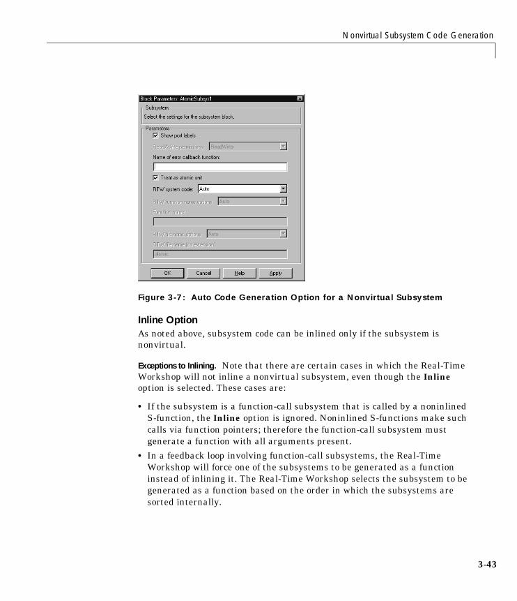
Nonvirtual Subsystem Code Generation
3-43
Figure 3-7: Auto Code Generation Option for a Nonvirtual Subsystem
Inline OptionAs noted above, subsystem code can be inlined only if the subsystem isnonvirtual.
Exceptions to Inlining. Note that there are certain cases in which the Real-TimeWorkshop will not inline a nonvirtual subsystem, even though the Inlineoption is selected. These cases are:
• If the subsystem is a function-call subsystem that is called by a noninlinedS-function, the Inline option is ignored. Noninlined S-functions make suchcalls via function pointers; therefore the function-call subsystem mustgenerate a function with all arguments present.
• In a feedback loop involving function-call subsystems, the Real-TimeWorkshop will force one of the subsystems to be generated as a functioninstead of inlining it. The Real-Time Workshop selects the subsystem to begenerated as a function based on the order in which the subsystems aresorted internally.
3 Code Generation and the Build Process
3-44
• If a subsystem is called from an S-function block that sets the optionSS_OPTION_FORCE_NONINLINED_FCNCALL to TRUE, it will not be inlined. Thismay be the case when user-defined Asynchronous Interrupt blocks or TaskSynchronization blocks are required. Such blocks must be generated asfunctions. The VxWorks Asynchronous Interrupt and Task Synchronizationblocks, shipped with the Real-Time Workshop, use theSS_OPTION_FORCE_NONINLINED_FCNCALL option.
To generate inlined subsystem code:
1 Select the subsystem block. Then select Subsystem parameters from theSimulink Edit menu. The Block Parameters dialog opens, as shown inFigure 3-8.
Alternatively, you can open the Block Parameters dialog by:
- Shift-double-clicking on the Subsystem block
- Right-clicking on the Subsystem block and selecting Block parametersfrom the pop-up menu.
2 If the subsystem is virtual, select Treat as atomic unit as shown inFigure 3-8. This makes the subsystem atomic, and the RTW system codepop-up menu becomes enabled.
If the system is already nonvirtual, the RTW system code menu is alreadyenabled.
3 Select Inline from the RTW system code menu as shown in Figure 3-8.
4 Click Apply and close the dialog.
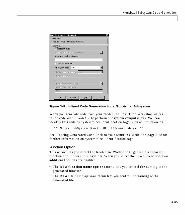
Nonvirtual Subsystem Code Generation
3-45
Figure 3-8: Inlined Code Generation for a Nonvirtual Subsystem
When you generate code from your model, the Real-Time Workshop writesinline code within model.c to perform subsystem computations. You canidentify this code by system/block identification tags, such as the following.
/* Atomic SubSystem Block: <Root>/AtomicSubsys1 */
See “Tracing Generated Code Back to Your Simulink Model” on page 3-28 forfurther information on system/block identification tags.
Function OptionThis option lets you direct the Real-Time Workshop to generate a separatefunction and file for the subsystem. When you select the Function option, twoadditional options are enabled:
• The RTW function name options menu lets you control the naming of thegenerated function.
• The RTW file name options menu lets you control the naming of thegenerated file.
3 Code Generation and the Build Process
3-46
Figure 3-9 shows the Block Parameters dialog with the Function optionselected.
RTW Function Name Options Menu. This menu offers the following choices:
• Auto: the Real-Time Workshop assigns a unique function name using thedefault naming convention: model_systemid(), where systemid is asequential identifier (s0, s1,...sn) assigned by Simulink.
• UseSubSystemName: the Real-Time Workshop uses the subsystem name asthe filename.
• UserSpecified: When this option is selected, the RTW function name textentry field is enabled. Enter any legal function name. Note that the functionname must be unique.
RTW File Name Options Menu. This menu offers the following choices:
• Auto: the Real-Time Workshop assigns a unique filename using the defaultnaming convention: model_systemid.c, where systemid is a sequentialidentifier (s0, s1,...sn) assigned by Simulink.
• UseSubSystemName: the Real-Time Workshop uses the subsystem name asthe filename.
• UseFunctionName: the Real-Time Workshop uses the function name (asspecified by the RTW function name options) as the filename.
• UserSpecified: When this option is selected, the RTW file name (noextension) text entry field is enabled. Enter any filename desired, but do notinclude the .c (or any other) extension. Note that this filename should beunique.
To generate a separate subsystem function and file:
1 Select the subsystem block. Then select Subsystem parameters from theSimulink Edit menu. The Block Parameters dialog opens, as shown inFigure 3-9.
Alternatively, you can open the Block Parameters dialog by:
- Shift-double-clicking on the Subsystem block
- Right-clicking on the Subsystem block and selecting Block parametersfrom the pop-up menu.
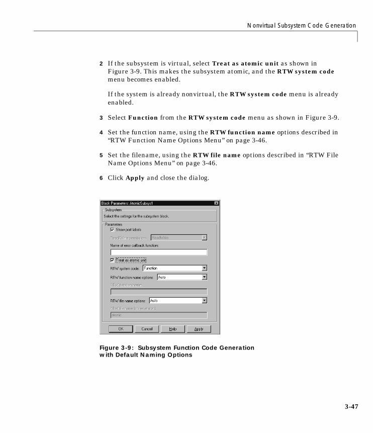
Nonvirtual Subsystem Code Generation
3-47
2 If the subsystem is virtual, select Treat as atomic unit as shown inFigure 3-9. This makes the subsystem atomic, and the RTW system codemenu becomes enabled.
If the system is already nonvirtual, the RTW system code menu is alreadyenabled.
3 Select Function from the RTW system code menu as shown in Figure 3-9.
4 Set the function name, using the RTW function name options described in“RTW Function Name Options Menu” on page 3-46.
5 Set the filename, using the RTW file name options described in “RTW FileName Options Menu” on page 3-46.
6 Click Apply and close the dialog.
Figure 3-9: Subsystem Function Code Generationwith Default Naming Options

3 Code Generation and the Build Process
3-48
Modularity of Subsystem CodeNote that code generated from nonvirtual subsystems, when written toseparate files, is not completely independent of the generating model. Forexample, subsystem code may reference global data structures of the model.Each subsystem code file contains appropriate include directives andcomments explaining the dependencies.

Generating Code and Executables from Subsystems
3-49
Generating Code and Executables from SubsystemsThe Real-Time Workshop can generate code and build an executable from anysubsystem within a model. The code generation and build process uses the codegeneration and build parameters of the root model.
To generate code and build an executable from a subsystem:
1 Set up the desired code generation and build parameters in the SimulationParameters dialog, just as you would for code generation from a model.
2 Select the desired subsystem block.
3 Right-click on the subsystem block and select Build Subsystem from theReal-Time Workshop submenu of the subsystem block’s context menu.
Alternatively, you can select Build Subsystem from the Real-TimeWorkshop submenu of the Tools menu. This menu item is enabled when asubsystem is selected in the current model.
4 A window displaying a list of the subsystem parameters opens. You candeclare any parameter to be tunable by selecting its check box in theTunable column.)
In the illustration above, the parameter K is declared tunable.
5 After selecting tunable parameters, click the Proceed button. This initiatesthe code generation and build process.
6 The build process displays status messages in the MATLAB commandwindow. When the build completes, the generated executable is in your
3 Code Generation and the Build Process
3-50
working directory. The name of the generated executable is subsystem.exe(PC) or subsystem (UNIX), where subsystem is the name of the sourcesubsystem block.
The generated code is in a build subdirectory, namedsubsystem_target_rtw, where subsystem is the name of the sourcesubsystem block and target is the name of the target configuration.
Note You can generate subsystem code using any target configurationavailable in the System Target File Browser. However, if the S-function targetis selected, Build Subsystem behaves identically to Generate S-function.(See “Automated S-Function Generation” on page 10-12.)

Parameters: Storage, Interfacing, and Tuning
3-51
Parameters: Storage, Interfacing, and TuningSimulink external mode (see Chapter 5, “External Mode”) offers a quick andeasy way to monitor signals and modify parameter values while generatedmodel code executes. However, external mode may not be appropriate for yourapplication in some cases. Some targets (such as the Real-Time WorkshopEmbedded Coder) do not support external mode. In other cases, you may wantyour existing code to access parameters and signals of a model directly, ratherthan using the external mode communications mechanism.
This section discusses how the Real-Time Workshop generates parameterstorage declarations, and how you can generate the storage declarations youneed to interface block parameters to your code.
Storage of Nontunable ParametersBy default, block parameters are not tunable in the generated code. In thedefault case, the Real-Time Workshop has control of parameter storagedeclarations and the symbolic naming of parameters in the generated code.
Nontunable parameters are stored as fields of a model-specific globalparameter data structure called rtP. The Real-Time Workshop initializes eachfield of rtP to the value of the corresponding block parameter at codegeneration time.
When the Inline parameters option is on, block parameters are evaluated atcode generation time, and their values appear as constants in the generatedcode. (A vector parameter, however, may be represented as an array ofconstants within rtP.)
As an example of nontunable parameter storage, consider this model.

3 Code Generation and the Build Process
3-52
The workspace variable Kp sets the gain of the Gain1 block.
Assume that Kp is nontunable, and has a value of 5.0. Table 3-2 shows thevariable declarations and the code generated for Kp in the noninlined andinlined cases.
Notice that the generated code does not preserve the symbolic name Kp. Thenoninlined code represent the gain of the Gain1 block as rtP.Gain1_Gain.
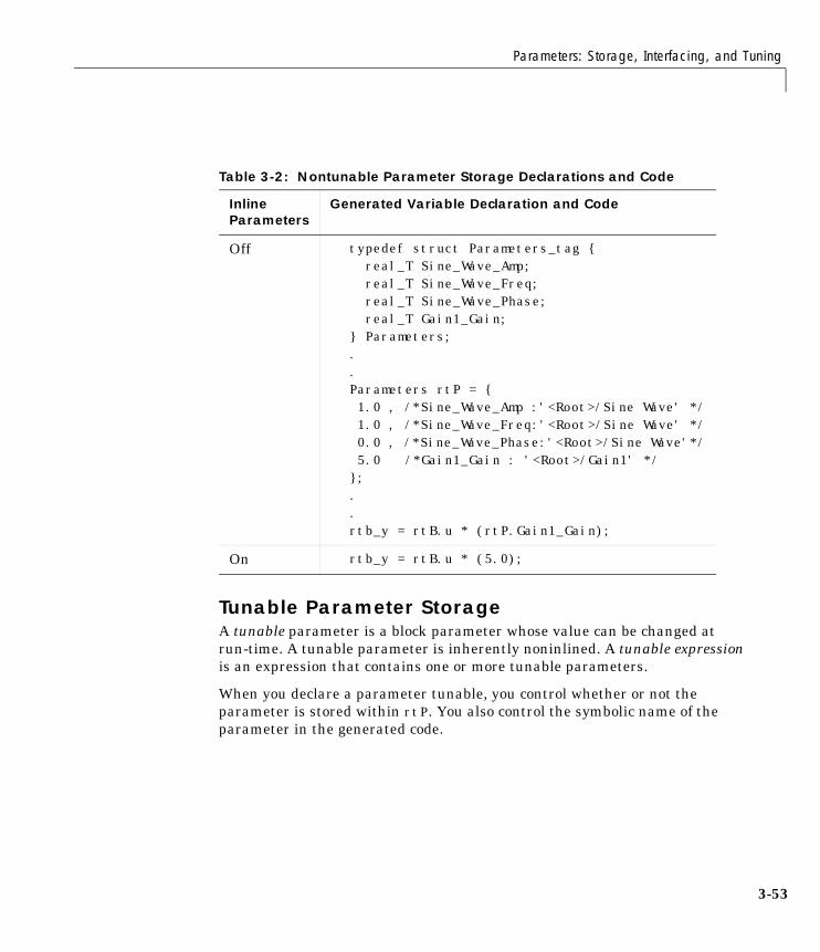
Parameters: Storage, Interfacing, and Tuning
3-53
Tunable Parameter StorageA tunable parameter is a block parameter whose value can be changed atrun-time. A tunable parameter is inherently noninlined. A tunable expressionis an expression that contains one or more tunable parameters.
When you declare a parameter tunable, you control whether or not theparameter is stored within rtP. You also control the symbolic name of theparameter in the generated code.
Table 3-2: Nontunable Parameter Storage Declarations and Code
Inline Parameters
Generated Variable Declaration and Code
Off typedef struct Parameters_tag {real_T Sine_Wave_Amp; real_T Sine_Wave_Freq;real_T Sine_Wave_Phase;real_T Gain1_Gain;
} Parameters;..Parameters rtP = {1.0 , /*Sine_Wave_Amp :'<Root>/Sine Wave' */1.0 , /*Sine_Wave_Freq:'<Root>/Sine Wave' */0.0 , /*Sine_Wave_Phase:'<Root>/Sine Wave'*/5.0 /*Gain1_Gain : '<Root>/Gain1' */};..rtb_y = rtB.u * (rtP.Gain1_Gain);
On rtb_y = rtB.u * (5.0);
3 Code Generation and the Build Process
3-54
When you declare a parameter tunable, you specify:
• The storage class of the parameter.
In the Real-Time Workshop, the storage class property of a parameterspecifies how the Real-Time Workshop declares the parameter in generatedcode.
Note that the term “storage class,” as used in the Real-Time Workshop, is notsynonymous with the term storage class specifier, as used in the C language.
• A storage type qualifier, such as const or volatile. This is simply an stringthat is included in the variable declaration, without error checking.
• (Implicitly) the symbolic name of the variable or field in which the parameteris stored. The Real-Time Workshop derives variable and field names fromthe names of tunable parameters.
The Real-Time Workshop generates a variable or struct storage declarationfor each tunable parameter. Your choice of storage class controls whether theparameter is declared as a member of rtP or as a separate global variable.
You can use the generated storage declaration to make the variable visible toyour code. You can also make variables declared in your code visible to thegenerated code. You are responsible for properly linking your code to generatedcode modules.
You can use tunable parameters or expressions in your root model and inmasked or unmasked subsystems, subject to certain restrictions (See “TunableExpressions” on page 3-61.)
To declare tunable parameters, you must first enable the Inline parametersoption. You then use the Model Parameter Configuration dialog to removeindividual parameters from inlining and declare them to be tunable. Thisallows you to improve overall efficiency by inlining most parameters, while atthe same time retaining the flexibility of run-time tuning for selectedparameters.
The mechanics of declaring tunable parameters is discussed in “Using theModel Parameter Configuration Dialog” on page 3-57.
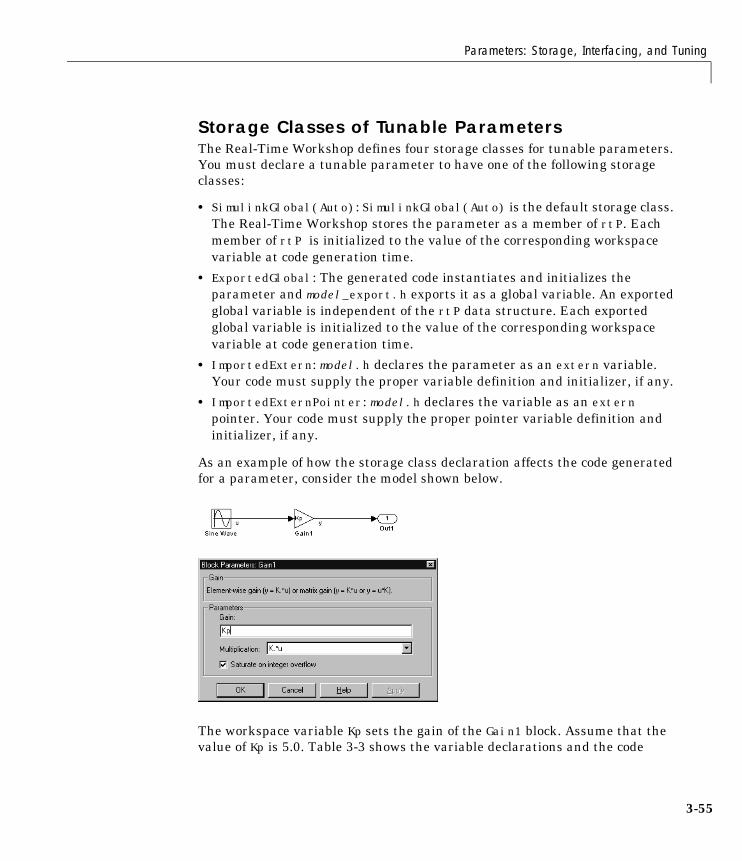
Parameters: Storage, Interfacing, and Tuning
3-55
Storage Classes of Tunable ParametersThe Real-Time Workshop defines four storage classes for tunable parameters.You must declare a tunable parameter to have one of the following storageclasses:
• SimulinkGlobal(Auto): SimulinkGlobal(Auto) is the default storage class.The Real-Time Workshop stores the parameter as a member of rtP. Eachmember of rtP is initialized to the value of the corresponding workspacevariable at code generation time.
• ExportedGlobal: The generated code instantiates and initializes theparameter and model_export.h exports it as a global variable. An exportedglobal variable is independent of the rtP data structure. Each exportedglobal variable is initialized to the value of the corresponding workspacevariable at code generation time.
• ImportedExtern: model.h declares the parameter as an extern variable.Your code must supply the proper variable definition and initializer, if any.
• ImportedExternPointer: model.h declares the variable as an externpointer. Your code must supply the proper pointer variable definition andinitializer, if any.
As an example of how the storage class declaration affects the code generatedfor a parameter, consider the model shown below.
The workspace variable Kp sets the gain of the Gain1 block. Assume that thevalue of Kp is 5.0. Table 3-3 shows the variable declarations and the code
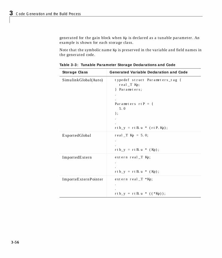
3 Code Generation and the Build Process
3-56
generated for the gain block when Kp is declared as a tunable parameter. Anexample is shown for each storage class.
Note that the symbolic name Kp is preserved in the variable and field names inthe generated code.
Table 3-3: Tunable Parameter Storage Declarations and Code
Storage Class Generated Variable Declaration and Code
SimulinkGlobal(Auto) typedef struct Parameters_tag {real_T Kp;
} Parameters;..Parameters rtP = {5.0
};..rtb_y = rtB.u * (rtP.Kp);
ExportedGlobal real_T Kp = 5.0;..rtb_y = rtB.u * (Kp);
ImportedExtern extern real_T Kp;..rtb_y = rtB.u * (Kp);
ImporteExternPointer extern real_T *Kp; ..rtb_y = rtB.u * ((*Kp));
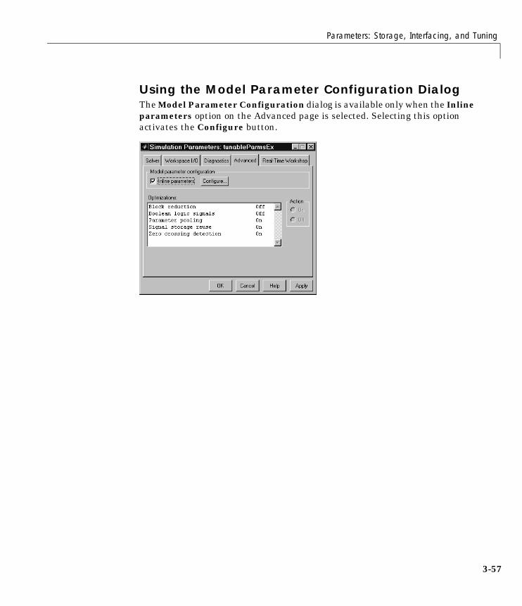
Parameters: Storage, Interfacing, and Tuning
3-57
Using the Model Parameter Configuration DialogThe Model Parameter Configuration dialog is available only when the Inlineparameters option on the Advanced page is selected. Selecting this optionactivates the Configure button.
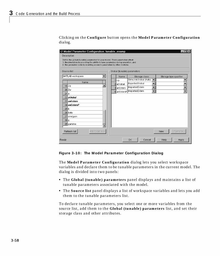
3 Code Generation and the Build Process
3-58
Clicking on the Configure button opens the Model Parameter Configurationdialog.
Figure 3-10: The Model Parameter Configuration Dialog
The Model Parameter Configuration dialog lets you select workspacevariables and declare them to be tunable parameters in the current model. Thedialog is divided into two panels:
• The Global (tunable) parameters panel displays and maintains a list oftunable parameters associated with the model.
• The Source list panel displays a list of workspace variables and lets you addthem to the tunable parameters list.
To declare tunable parameters, you select one or more variables from thesource list, add them to the Global (tunable) parameters list, and set theirstorage class and other attributes.
Parameters: Storage, Interfacing, and Tuning
3-59
Source List Panel. The Source list panel displays a menu and a scrolling table ofnumerical workspace variables.
The menu lets you choose the source of the variables to be displayed in the list.Currently there is only one choice: MATLAB workspace. The source listdisplays names of the variables defined in the MATLAB base workspace.
Selecting one or more variables from the source list enables the Add to tablebutton. Clicking Add to table adds selected variables to the tunableparameters list in the Global (tunable) parameters panel. This action is allthat is necessary to declare tunable parameters.
In the source list, the names of variables that have been added to the tunableparameters list are displayed in italics (See Figure 3-10).
The Refresh list button updates the table of variables to reflect the currentstate of the workspace. If you define or remove variables in the workspacewhile the Model Parameter Configuration dialog is open, click the Refreshlist button when you return to the dialog. The new variables are added to thesource list.
Global (Tunable) Parameters Panel. The Global (tunable) parameters paneldisplays a scrolling table of variables that have been declared tunable in thecurrent model, and lets you specify their attributes. The Global (tunable)parameters panel also lets you remove entries from the list, or create newtunable parameters.
You select individual variables and change their attributes directly in thetable. The attributes are:
• Storage class of the parameter in the generated code. Select one of
- SimulinkGlobal(Auto)
- ExportedGlobal- ImportedExtern
- ImportedExternPointer
See “Storage Classes of Tunable Parameters” on page 3-55 for definitions.
• Storage type qualifier of the variable in the generated code. For variableswith any storage class except SimulinkGlobal(Auto), you can add a qualifier(such as const or volatile) to the generated storage declaration. To do so,you can select a predefined qualifier from the list, or add additional qualifiersto the list. Note that the code generator does not check the storage type
3 Code Generation and the Build Process
3-60
qualifier for validity. The code generator includes the qualifier string in thegenerated code without syntax checking.
• Name of the parameter. This field is used only when creating a new tunablevariable.
The Remove button deletes selected variables from the Global (tunable)parameters list.
The New button lets you create new tunable variables in the Global (tunable)parameters list. At a later time, you can add references to these variables inthe model.
If the name you enter matches the name of an existing workspace variable inthe Source list, that variable is declared tunable, and is displayed in italics inthe Source list.
To define a new tunable variable, click the New button. This creates an emptyentry in the table. Then, enter the name and attributes of the variable and clickApply.
Note If you edit the name of an existing variable in the list, you actuallycreate a new tunable variable with the new name. The previous variable isremoved from the list and loses its tunability (that is, it is inlined).
Declaring Tunable VariablesTo declare an existing variable tunable:
1 Open the Model Parameter Configuration dialog.
2 In the Source list panel, click on the desired variable in the list to select it.
3 Click the Add to table button. The variable then appears in the table oftunable variables in the Global (tunable) parameters panel.
4 Click on the variable in the Global (tunable) parameters panel.
5 Select the desired storage class from the Storage class menu.
6 Optionally, select (or enter) a storage type qualifier.
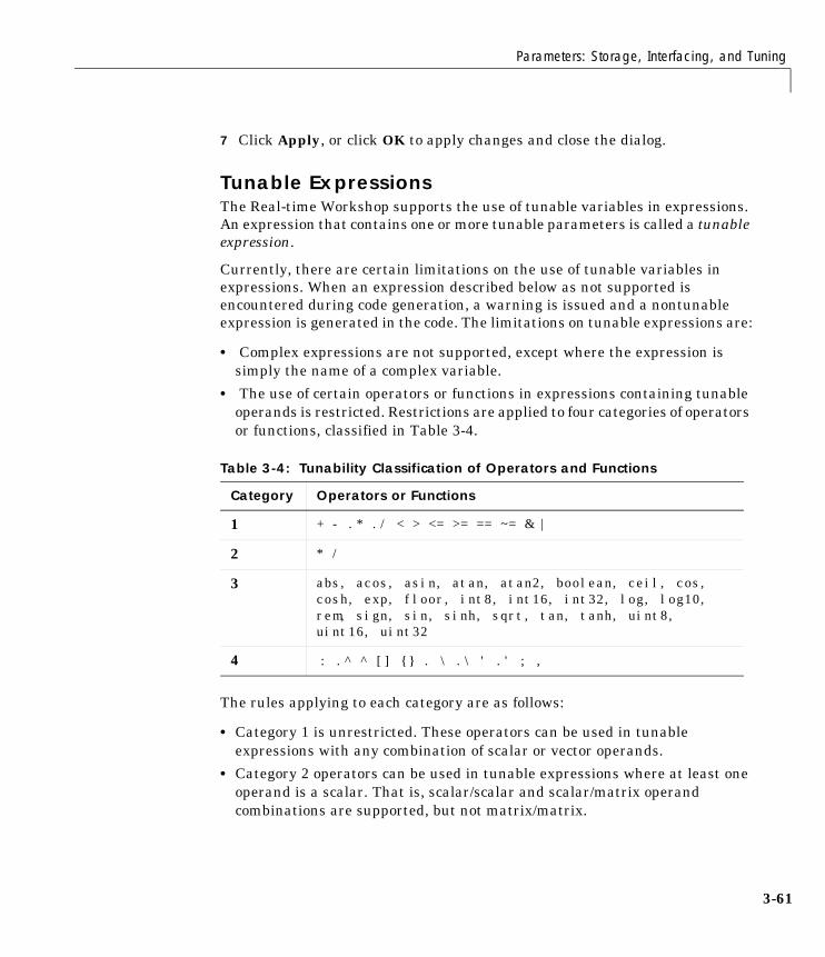
Parameters: Storage, Interfacing, and Tuning
3-61
7 Click Apply, or click OK to apply changes and close the dialog.
Tunable ExpressionsThe Real-time Workshop supports the use of tunable variables in expressions.An expression that contains one or more tunable parameters is called a tunableexpression.
Currently, there are certain limitations on the use of tunable variables inexpressions. When an expression described below as not supported isencountered during code generation, a warning is issued and a nontunableexpression is generated in the code. The limitations on tunable expressions are:
• Complex expressions are not supported, except where the expression issimply the name of a complex variable.
• The use of certain operators or functions in expressions containing tunableoperands is restricted. Restrictions are applied to four categories of operatorsor functions, classified in Table 3-4.
The rules applying to each category are as follows:
• Category 1 is unrestricted. These operators can be used in tunableexpressions with any combination of scalar or vector operands.
• Category 2 operators can be used in tunable expressions where at least oneoperand is a scalar. That is, scalar/scalar and scalar/matrix operandcombinations are supported, but not matrix/matrix.
Table 3-4: Tunability Classification of Operators and Functions
Category Operators or Functions
1 + - .* ./ < > <= >= == ~= & |
2 * /
3 abs, acos, asin, atan, atan2, boolean, ceil, cos, cosh, exp, floor, int8, int16, int32, log, log10, rem, sign, sin, sinh, sqrt, tan, tanh, uint8, uint16, uint32
4 : .^ ^ [] {} . \ .\ ' .' ; ,
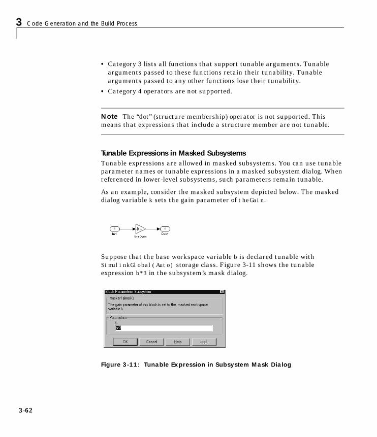
3 Code Generation and the Build Process
3-62
• Category 3 lists all functions that support tunable arguments. Tunablearguments passed to these functions retain their tunability. Tunablearguments passed to any other functions lose their tunability.
• Category 4 operators are not supported.
Note The “dot” (structure membership) operator is not supported. Thismeans that expressions that include a structure member are not tunable.
Tunable Expressions in Masked SubsystemsTunable expressions are allowed in masked subsystems. You can use tunableparameter names or tunable expressions in a masked subsystem dialog. Whenreferenced in lower-level subsystems, such parameters remain tunable.
As an example, consider the masked subsystem depicted below. The maskeddialog variable k sets the gain parameter of theGain.
Suppose that the base workspace variable b is declared tunable withSimulinkGlobal(Auto) storage class. Figure 3-11 shows the tunableexpression b*3 in the subsystem’s mask dialog.
Figure 3-11: Tunable Expression in Subsystem Mask Dialog
Parameters: Storage, Interfacing, and Tuning
3-63
The Real-Time Workshop produces the following output computation fortheGain.
/* Gain Block: <S1>/theGain */rtb_temp0 *= (rtP.b * 3.0);
Note that b is represented as a member of the global parameters structure, rtP.
Limitations of Tunable Expressions in Masked Subsystems. Expressions that includevariables that were declared or modified in mask initialization code are nottunable.
As an example, consider the subsystem above, modified as follows:
• The mask initialization code ist = 3 * k;
• The parameter k of the myGain block is 4 + t.
• Workspace variable b = 2. The expression b * 3 is plugged into the maskdialog as in Figure 3-11.
Since the mask initialization code can only run once, k is evaluated at codegeneration time as
4 + (3 * (2 * 3) )
The Real-Time Workshop inlines the result. Therefore, despite the fact that bwas declared tunable, the code generator produces the following outputcomputation for theGain.
/* Gain Block: <S1>/theGain */rtb_temp0 *= (22.0);
Tunability of Linear Block ParametersThe following blocks have a Realization parameter that affects the tunabilityof their parameters:
• Transfer Fcn
• State-Space,
• Discrete Transfer Fcn,
• Discrete State-Space
3 Code Generation and the Build Process
3-64
• Discrete Filter
The Realization parameter must be set via the MATLAB set_param command, as in the following example.
set_param(gcb,'Realization','auto')
The following values are defined for the Realization parameter:
• general: The block's parameters are preserved in the generated code,permitting parameters to be tuned.
• sparse: The block's parameters are represented in the code by transformedvalues that increase the computational efficiency. Because of thetransformation, the block’s parameters are no longer tunable.
• auto: This setting is the default. A general realization is used if one or moreof the block's parameters are tunable. Otherwise sparse, is used.
Note To tune the parameter values of a block of one of the above typeswithout restriction during an external mode simulation, you must use setRealization to general .
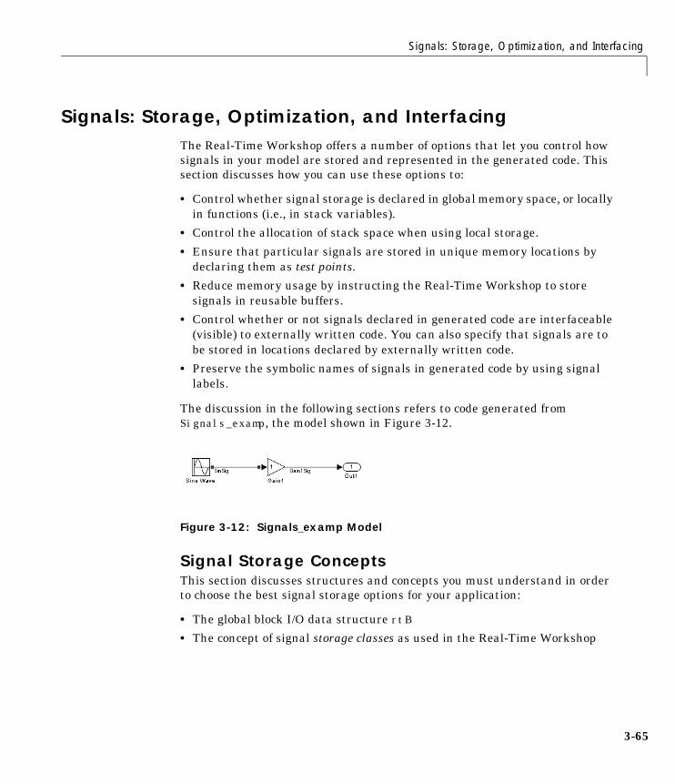
Signals: Storage, Optimization, and Interfacing
3-65
Signals: Storage, Optimization, and InterfacingThe Real-Time Workshop offers a number of options that let you control howsignals in your model are stored and represented in the generated code. Thissection discusses how you can use these options to:
• Control whether signal storage is declared in global memory space, or locallyin functions (i.e., in stack variables).
• Control the allocation of stack space when using local storage.
• Ensure that particular signals are stored in unique memory locations bydeclaring them as test points.
• Reduce memory usage by instructing the Real-Time Workshop to storesignals in reusable buffers.
• Control whether or not signals declared in generated code are interfaceable(visible) to externally written code. You can also specify that signals are tobe stored in locations declared by externally written code.
• Preserve the symbolic names of signals in generated code by using signallabels.
The discussion in the following sections refers to code generated fromSignals_examp, the model shown in Figure 3-12.
Figure 3-12: Signals_examp Model
Signal Storage ConceptsThis section discusses structures and concepts you must understand in orderto choose the best signal storage options for your application:
• The global block I/O data structure rtB
• The concept of signal storage classes as used in the Real-Time Workshop
3 Code Generation and the Build Process
3-66
rtB: the Global Block I/O StructureBy default, the Real-Time Workshop attempts to optimize memory usage bysharing signal memory and using local variables.
However, there are a number of circumstances in which it is desirable ornecessary to place signals in global memory. For example:
• You may want a signal to be stored in a structure that is visible to externallywritten code.
• The number and/or size of signals in your model may exceed the stack spaceavailable for local variables.
In such cases, it is possible to override the default behavior and store selected(or all) signals in a model-specific global block I/O data structure. The globalblock I/O structure is called rtB.
The following code fragment illustrates how rtB is defined and declared in codegenerated (with signal storage optimizations off) from the Signals_exampmodel shown in Figure 3-12.
typedef struct BlockIO_tag {real_T SinSig; /* <Root>/Sine Wave */real_T Gain1Sig; /* <Root>/Gain1 */
} BlockIO;.../* Block I/O Structure */BlockIO rtB;
Field names for signals stored in rtB are generated according to the rulesdescribed in “Symbolic Naming Conventions for Signals in Generated Code” onpage 3-74.
Storage Classes for SignalsIn the Real-Time Workshop, the storage class property of a signal specifies howthe Real-Time Workshop declares and stores the signal. In some cases thisspecification is qualified by further options.
Note that in the context of the Real-Time Workshop, the term “storage class” isnot synonymous with the term storage class specifier, as used in the Clanguage.

Signals: Storage, Optimization, and Interfacing
3-67
Default Storage Class. Auto is the default storage class. Auto is the appropriatestorage class for signals that you do not need to interface to external code.Signals with Auto storage class may be stored in local and/or shared variables,or in a global data structure. The form of storage depends on the Signalstorage reuse and Local block outputs options, and on available stack space.See “Signals with Auto Storage Class” on page 3-68 for a full description of codegeneration options for signals with Auto storage class.
Explicitly Assigned Storage Classes. Signals with storage classes other than Autoare stored either as members of rtB, or in unstructured global variables,independent of rtB. These storage classes are appropriate for signals that youwant to monitor and/or interface to external code.
The Signal storage reuse and Local block outputs optimizations do not applyto signals with storage classes other than Auto.
Use the Signal Properties dialog to assign these storage classes to signals:
• SimulinkGlobal(Test Point): Test points are stored as fields of the rtBstructure that are not shared or reused by any other signal. See “DeclaringTest Points” on page 3-71 for further information.
• ExportedGlobal: The signal is stored in a global variable, independent of thertB data structure. model_export.h exports the variable. Signals withExportedGlobal storage class must have unique signal names. See“Interfacing Signals to External Code” on page 3-72 for further information.
• ImportedExtern: model.h declares the signal as an extern variable. Yourcode must supply the proper variable definition. Signals withImportedExtern storage class must have unique signal names. See“Interfacing Signals to External Code” on page 3-72 for further information.
• ImportedExternPointer: model.h declares the signal as an extern pointer.Your code must supply the proper pointer variable definition. Signals withImportedExtern storage class must have unique signal names. See“Interfacing Signals to External Code” on page 3-72 for further information.
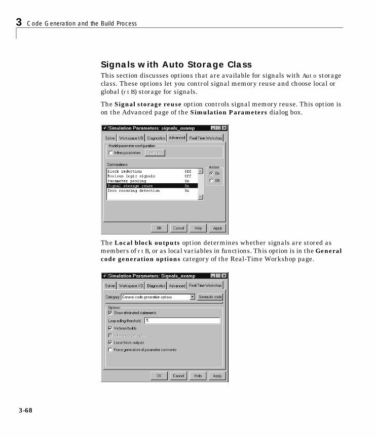
3 Code Generation and the Build Process
3-68
Signals with Auto Storage ClassThis section discusses options that are available for signals with Auto storageclass. These options let you control signal memory reuse and choose local orglobal (rtB) storage for signals.
The Signal storage reuse option controls signal memory reuse. This option ison the Advanced page of the Simulation Parameters dialog box.
The Local block outputs option determines whether signals are stored asmembers of rtB, or as local variables in functions. This option is in the Generalcode generation options category of the Real-Time Workshop page.
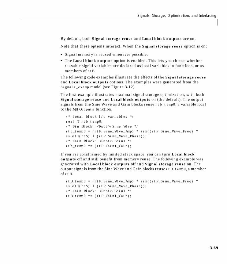
Signals: Storage, Optimization, and Interfacing
3-69
By default, both Signal storage reuse and Local block outputs are on.
Note that these options interact. When the Signal storage reuse option is on:
• Signal memory is reused whenever possible.
• The Local block outputs option is enabled. This lets you choose whetherreusable signal variables are declared as local variables in functions, or asmembers of rtB.
The following code examples illustrate the effects of the Signal storage reuseand Local block outputs options. The examples were generated from theSignals_examp model (see Figure 3-12).
The first example illustrates maximal signal storage optimization, with bothSignal storage reuse and Local block outputs on (the default). The outputsignals from the Sine Wave and Gain blocks reuse rtb_temp0, a variable localto the MdlOutputs function.
/* local block i/o variables */real_T rtb_temp0;/* Sin Block: <Root>/Sine Wave */rtb_temp0 = (rtP.Sine_Wave_Amp) * sin((rtP.Sine_Wave_Freq) * ssGetT(rtS) + (rtP.Sine_Wave_Phase));/* Gain Block: <Root>/Gain1 */rtb_temp0 *= (rtP.Gain1_Gain);
If you are constrained by limited stack space, you can turn Local blockoutputs off and still benefit from memory reuse. The following example wasgenerated with Local block outputs off and Signal storage reuse on. Theoutput signals from the Sine Wave and Gain blocks reuse rtB.temp0, a memberof rtB.
rtB.temp0 = (rtP.Sine_Wave_Amp) * sin((rtP.Sine_Wave_Freq) * ssGetT(rtS) + (rtP.Sine_Wave_Phase));/* Gain Block: <Root>/Gain1 */rtB.temp0 *= (rtP.Gain1_Gain);
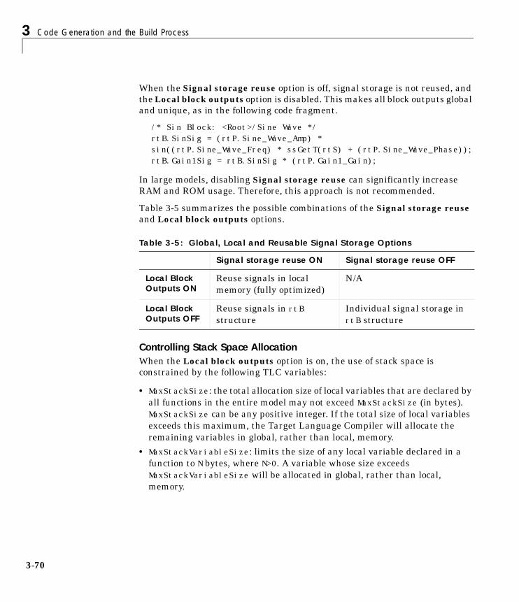
3 Code Generation and the Build Process
3-70
When the Signal storage reuse option is off, signal storage is not reused, andthe Local block outputs option is disabled. This makes all block outputs globaland unique, as in the following code fragment.
/* Sin Block: <Root>/Sine Wave */rtB.SinSig = (rtP.Sine_Wave_Amp) *sin((rtP.Sine_Wave_Freq) * ssGetT(rtS) + (rtP.Sine_Wave_Phase));rtB.Gain1Sig = rtB.SinSig * (rtP.Gain1_Gain);
In large models, disabling Signal storage reuse can significantly increaseRAM and ROM usage. Therefore, this approach is not recommended.
Table 3-5 summarizes the possible combinations of the Signal storage reuseand Local block outputs options.
Controlling Stack Space AllocationWhen the Local block outputs option is on, the use of stack space isconstrained by the following TLC variables:
• MaxStackSize: the total allocation size of local variables that are declared byall functions in the entire model may not exceed MaxStackSize (in bytes).MaxStackSize can be any positive integer. If the total size of local variablesexceeds this maximum, the Target Language Compiler will allocate theremaining variables in global, rather than local, memory.
• MaxStackVariableSize: limits the size of any local variable declared in afunction to N bytes, where N>0. A variable whose size exceedsMaxStackVariableSize will be allocated in global, rather than local,memory.
Table 3-5: Global, Local and Reusable Signal Storage Options
Signal storage reuse ON Signal storage reuse OFF
Local BlockOutputs ON
Reuse signals in localmemory (fully optimized)
N/A
Local BlockOutputs OFF
Reuse signals in rtBstructure
Individual signal storage inrtB structure
Signals: Storage, Optimization, and Interfacing
3-71
You can change the values of these variables in your system target file ifnecessary. See “Assigning Target Language Compiler Variables” on page 3-93for further information.
Declaring Test PointsA test point is a signal that is stored in a unique location that is not shared orreused by any other signal. Test-pointing is the process of declaring a signal tobe a test point.
Test points are stored as members of the rtB structure, even when the Signalstorage reuse and Local block outputs option are selected. Test-pointing letsyou override these options for individual signals. Therefore, you can test-pointselected signals, without losing the benefits of optimized storage for the othersignals in your model.
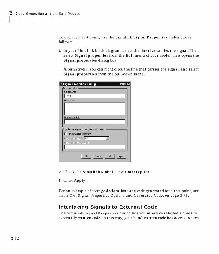
3 Code Generation and the Build Process
3-72
To declare a test point, use the Simulink Signal Properties dialog box asfollows:
1 In your Simulink block diagram, select the line that carries the signal. Thenselect Signal properties from the Edit menu of your model. This opens theSignal properties dialog box.
Alternatively, you can right-click the line that carries the signal, and selectSignal properties from the pull-down menu.
2 Check the SimulinkGlobal (Test Point) option.
3 Click Apply.
For an example of storage declarations and code generated for a test point, seeTable 3-6, Signal Properties Options and Generated Code, on page 3-76.
Interfacing Signals to External CodeThe Simulink Signal Properties dialog lets you interface selected signals toexternally written code. In this way, your hand-written code has access to such
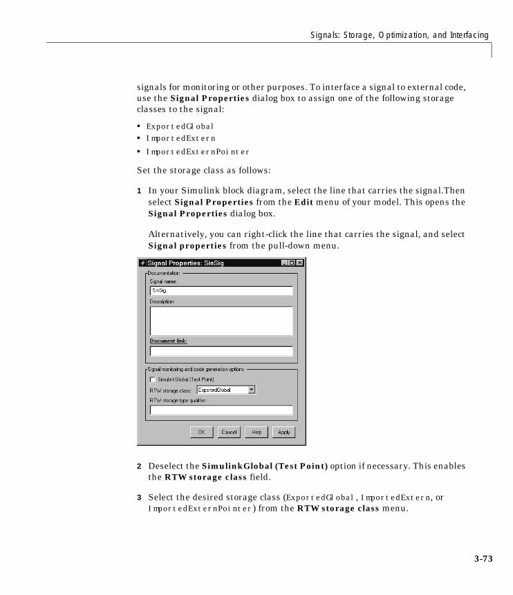
Signals: Storage, Optimization, and Interfacing
3-73
signals for monitoring or other purposes. To interface a signal to external code,use the Signal Properties dialog box to assign one of the following storageclasses to the signal:
• ExportedGlobal• ImportedExtern
• ImportedExternPointer
Set the storage class as follows:
1 In your Simulink block diagram, select the line that carries the signal.Thenselect Signal Properties from the Edit menu of your model. This opens theSignal Properties dialog box.
Alternatively, you can right-click the line that carries the signal, and selectSignal properties from the pull-down menu.
2 Deselect the SimulinkGlobal (Test Point) option if necessary. This enablesthe RTW storage class field.
3 Select the desired storage class (ExportedGlobal, ImportedExtern, orImportedExternPointer) from the RTW storage class menu.

3 Code Generation and the Build Process
3-74
4 Optional: For storage classes other than Auto and SimulinkGlobal, you canenter a storage type qualifier such as const or volatile in the RTW storagetype qualifier field. Note that the Real-Time Workshop does not check thisstring for errors; whatever you enter is included in the variable declaration.
5 Click Apply.
Note You can also interface test points and other signals that are stored asmembers of rtB to your code. To do this, your code must know the address ofthe rtB structure where the data is stored, and other information. Thisinformation is not automatically exported. The Real-Time Workshop providesC and Target Language Compiler APIs that give your code access to rtB andother data structures. See “Interfacing Parameters and Signals” on page 17-65for further information.
Symbolic Naming Conventions for Signalsin Generated CodeWhen signals have a storage class other than Auto, the Real-Time Workshoppreserves symbolic information about the signals or their originating blocks inthe generated code.
For labelled signals, field names in rtB derive from the signal names. In thefollowing example, the field names rtB.SinSig and rtB.Gain1Sig derive fromthe corresponding labeled signals in the Signals_examp model (shown inFigure 3-12).
typedef struct BlockIO_tag {real_T SinSig; /* <Root>/Sine Wave */real_T Gain1Sig; /* <Root>/Gain1 */
} BlockIO;
For unlabeled signals, rtB field names derive from the name of the source blockor subsystem. The naming format is
rtB.system#_BlockName_outport#
where system# is a unique system number assigned by Simulink, BlockName isthe name of the source block, and outport# is a port number. The port number
Signals: Storage, Optimization, and Interfacing
3-75
(outport#) is used only when the source block or subsystem has multipleoutput ports.
When a signal has Auto storage class, the Real-Time Workshop controlsgeneration of variable or field names without regard to signal labels.

3 Code Generation and the Build Process
3-76
Summary of Signal Storage Class OptionsTable 3-6 shows, for each signal storage class option, the variable declarationand the code generated for Sine Wave output (SinSig) of the model shown inFigure 3-12.
Table 3-6: Signal Properties Options and Generated Code
Storage Class Declaration Code
Auto
(with storageoptimizationson)
real_T rtb_temp0;(declared inmodel_common.h)
rtb_temp0 = (rtP.Sine_Wave_Amp) * sin((rtP.Sine_Wave_Freq) * ssGetT(rtS) + (rtP.Sine_Wave_Phase));
Test point typedef struct BlockIO_tag {
real_T SinSig; real_T Gain1Sig;
} BlockIO;..BlockIO rtB;
rtB.SinSig = (rtP.Sine_Wave_Amp) * sin((rtP.Sine_Wave_Freq) * ssGetT(rtS) + (rtP.Sine_Wave_Phase));
ExportedGlobal
extern real_T SinSig;(declared inmodel_export.h
SinSig = (rtP.Sine_Wave_Amp) * sin((rtP.Sine_Wave_Freq) * ssGetT(rtS) + (rtP.Sine_Wave_Phase));
ImportedExtern
extern real_T SinSig;(declared inmodel_common.h)
SinSig = (rtP.Sine_Wave_Amp) * sin((rtP.Sine_Wave_Freq) * ssGetT(rtS) + (rtP.Sine_Wave_Phase));
ImportedExternPointer
extern real_T *SinSig;(declared inmodel_common.h)
*(SinSig) = (rtP.Sine_Wave_Amp) * sin((rtP.Sine_Wave_Freq) * ssGetT(rtS) + (rtP.Sine_Wave_Phase));
Signals: Storage, Optimization, and Interfacing
3-77
C API for Parameter Tuning and Signal MonitoringThe Real-Time Workshop includes support for development of a C applicationprogram interface (API) for tuning parameters and monitoring signalsindependent of external mode. See “Interfacing Parameters and Signals” inChapter 17 for information.
Target Language Compiler API for ParameterTuning and Signal MonitoringThe Real-Time Workshop includes support for development of a TargetLanguage Compiler API for tuning parameters and monitoring signalsindependent of external mode. See “Interfacing Parameters and Signals” inChapter 17 for information.
Parameter Tuning via MATLAB CommandsThe Model Parameter Configuration dialog is the recommended way to seeor set the attributes of tunable parameters. However, you can also useMATLAB get_param and set_param commands.
The following commands return the tunable parameters and/or theirattributes:
• get_param(gcs, 'TunableVars')• get_param(gcs, 'TunableVarsStorageClass')
• get_param(gcs, 'TunableVarsTypeQualifier')
The following commands declare tunable parameters or set their attributes:
• set_param(gcs, 'TunableVars', str)
The argument str (string) is a comma-separated list of variable names.• set_param(gcs, 'TunableVarsStorageClass', str)
The argument str (string) is a comma-separated list of storage classsettings.
The valid storage class settings are:- Auto- ExportedGlobal- ImportedExtern- ImportedExternPointer
3 Code Generation and the Build Process
3-78
• set_param(gcs, 'TunableVarsTypeQualifier', str)
The argument str (string) is a comma-separated list of storage typequalifiers.
The following example declares the variable k1 to be tunable, with storage classExportedGlobal and type qualifier const.
set_param(gcs, 'TunableVars', 'k1')set_param(gcs, 'ExportedGlobal')set_param(gcs, 'TunableVarsTypeQualifier','const')
Simulink Data Objects and Code Generation
3-79
Simulink Data Objects and Code Generation
PrerequisitesBefore using Simulink data objects with the Real-Time Workshop, please readthe following:
• The discussion of Simulink data objects in Using Simulink
• “Parameters: Storage, Interfacing, and Tuning” on page 3-51
• “Signals: Storage, Optimization, and Interfacing” on page 3-65
OverviewWithin the class hierarchy of Simulink data objects, Simulink provides twoclasses that are designed as base classes for signal and parameter storage.These are:
• Simulink.Parameter: Objects that are instances of the Simulink.Parameterclass or any class derived from Simulink.Parameter are called parameterobjects.
• Simulink.Signal: Objects that are instances of the Simulink.Signal classor any class derived from Simulink.Signal are called signal objects.
The RTWInfo properties of parameter and signal objects are used by theReal-Time Workshop during code generation. These properties let you assignstorage classes and storage type qualifiers to the objects, thereby controllinghow the generated code stores and represents signals and parameters.
The Real-Time Workshop also writes information about the properties ofparameter and signal objects to the model.rtw file. This information, formattedas ObjectProperties records, is accessible to Target Language Compilerprograms. For general information on ObjectProperties records, see “ObjectProperty Information in the model.rtw File” on page 3-88.
The general procedure for using Simulink data objects in code generation is asfollows:
1 Define a subclass of one of the built-in Simulink.Data classes.
- For parameters, define a subclass of Simulink.Parameter.
- For signals, define a subclass of Simulink.Signal.
3 Code Generation and the Build Process
3-80
2 Instantiate parameter or signal objects from your subclass and set theirproperties appropriately, using the Simulink Explorer.
3 Use the objects as parameters or signals within your model.
4 Generate code and build your target executable.
The following sections describe the relationship between Simulink data objectsand code generation in the Real-Time Workshop.

Simulink Data Objects and Code Generation
3-81
Parameter ObjectsThis section discusses how to use parameter objects in code generation.
Configuring Parameter Objects for Code GenerationIn configuring parameter objects for code generation, you use the followingcode generation and parameter object properties:
• The Inline parameters option (see “Parameters: Storage, Interfacing, andTuning” on page 3-51).
• Parameter object properties:
- Value. This property is the numeric value of the object, used as an initial(or inlined) parameter value in generated code.
- RTWInfo.StorageClass. This property controls the generated storagedeclaration and code for the parameter object.
- RTWInfo.TypeQualifier. This property is a string included as a prefix inthe generated storage declaration.
Other parameter object properties (such as user-defined properties of classesderived from Simulink.Parameter) do not affect code generation.
Note If Inline parameters is off (the default), the RTWInfo.StorageClassand RTWInfo.TypeQualifier parameter object properties are ignored in codegeneration.
Effect of Storage Classes on Code Generation for Parameter ObjectsThe Real-Time Workshop generates code and storage declarations based on theRTWInfo.StorageClass property of the parameter object. The logic is asfollows:
• If the storage class is 'Auto' (the default), the parameter object is inlined (ifpossible), using the Value property.
• For storage classes other than 'Auto', the parameter object is handled as atunable parameter.
- A global storage declaration is generated. You can use the generatedstorage declaration to make the variable visible to your hand-written code.
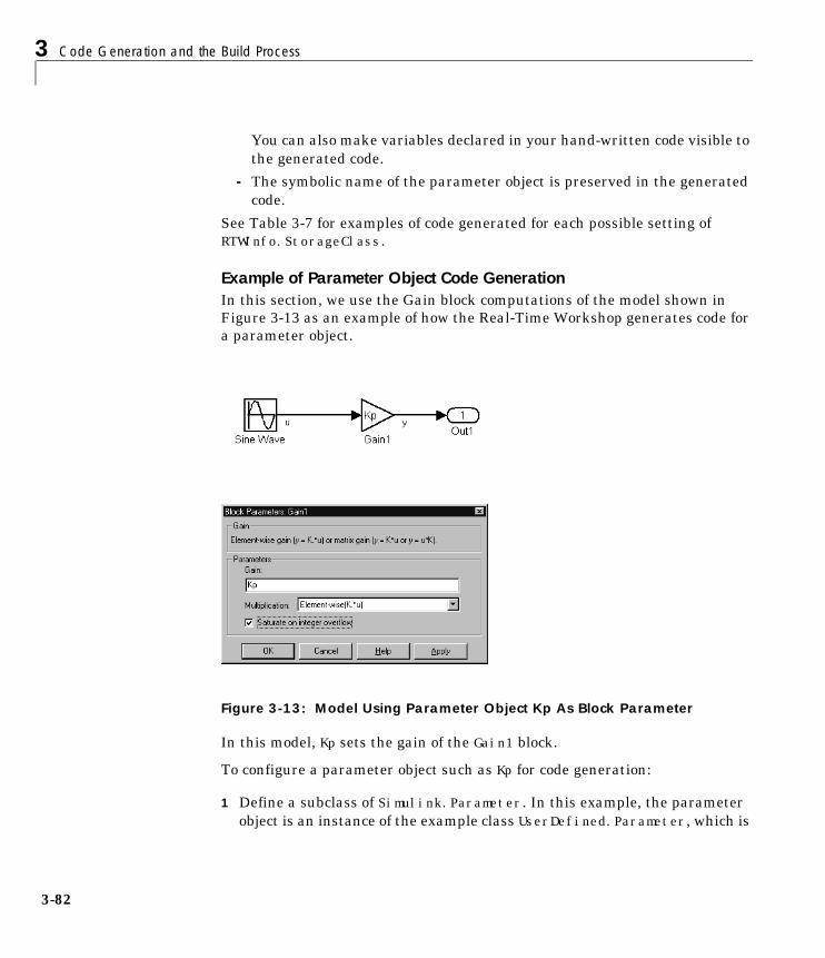
3 Code Generation and the Build Process
3-82
You can also make variables declared in your hand-written code visible tothe generated code.
- The symbolic name of the parameter object is preserved in the generatedcode.
See Table 3-7 for examples of code generated for each possible setting ofRTWInfo.StorageClass.
Example of Parameter Object Code GenerationIn this section, we use the Gain block computations of the model shown inFigure 3-13 as an example of how the Real-Time Workshop generates code fora parameter object.
Figure 3-13: Model Using Parameter Object Kp As Block Parameter
In this model, Kp sets the gain of the Gain1 block.
To configure a parameter object such as Kp for code generation:
1 Define a subclass of Simulink.Parameter. In this example, the parameterobject is an instance of the example class UserDefined.Parameter, which is
Simulink Data Objects and Code Generation
3-83
provided with Simulink. For the definition of UserDefined.Parameter, seethe directorymatlabroot/toolbox/simulink/simdemos/@UserDefined.
2 Instantiate a parameter object from your subclass. The following exampleinstantiates Kp as a parameter object of class UserDefined.Parameter.
Kp = UserDefined.Parameter;
Make sure that the name of the parameter object matches the desired blockparameter in your model. This ensures that Simulink can associate theparameter name with the correct object. For example, in the model ofFigure 3-13, the Gain block parameter Kp resolves to the parameter objectKp.
3 Set the object properties.
- Set the Value property, for example:Kp.Value = 5.0;
- Set the RTWInfo.StorageClass property, for example:Kp.RTWInfo.StorageClass = 'ExportedGlobal';
- Optional: if the RTWInfo.StorageClass property is not Auto, you canassign a storage type qualifier to the RTWInfo.TypeQualifier property,for example:Kp.RTWInfo.StorageClass = 'const';
Table 3-7 shows the variable declarations for Kp and the code generated for theGain block in the model shown in Figure 3-13, with Inline parameters on. Anexample is shown for each possible setting of RTWInfo.StorageClass.
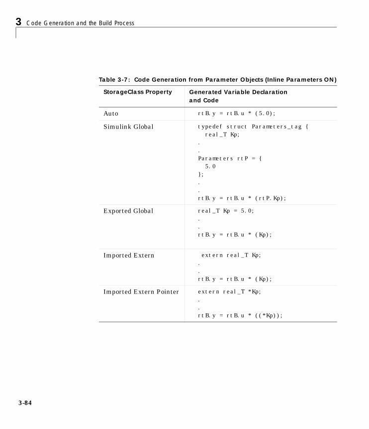
3 Code Generation and the Build Process
3-84
Table 3-7: Code Generation from Parameter Objects (Inline Parameters ON)
StorageClass Property Generated Variable Declarationand Code
Auto rtB.y = rtB.u * (5.0);
Simulink Global typedef struct Parameters_tag { real_T Kp;..Parameters rtP = { 5.0 };..rtB.y = rtB.u * (rtP.Kp);
Exported Global real_T Kp = 5.0;..rtB.y = rtB.u * (Kp);
Imported Extern extern real_T Kp;..rtB.y = rtB.u * (Kp);
Imported Extern Pointer extern real_T *Kp;..rtB.y = rtB.u * ((*Kp));
Simulink Data Objects and Code Generation
3-85
Signal ObjectsThis section discusses how to use signal objects in code generation.
Configuring Signal Objects for Code GenerationIn configuring signal objects for code generation, you use the following codegeneration options and signal object properties:
• The Signal storage reuse code generation option (see “Signals: Storage,Optimization, and Interfacing” on page 3-65).
• The Local block outputs code generation option (see “Signals: Storage,Optimization, and Interfacing” on page 3-65).
• Signal object properties:
- RTWInfo.StorageClass. The storage classes defined for signal objects, andtheir effect on code generation, are the same for model signals and signalobjects (see “Storage Classes for Signals” on page 3–66).
- RTWInfo.TypeQualifier. This property is a storage type qualifier. Thestring is included as a prefix in the generated storage declaration. Thesyntax of the string is not checked for validity.
Other signal object properties (such as user-defined properties of classesderived from Simulink.Signal) do not affect code generation.
Effect of Storage Classes on Code Generation for Signal ObjectsThe way in which the Real-Time Workshop uses storage classes to determinehow signals are stored is the same with and without signal objects. However,if a signal’s label resolves to a signal object, the object’s RTWInfo.StorageClassproperty is used in place of the port configuration of the signal.
The default storage class is Auto. If the storage type is Auto, the Real-TimeWorkshop follows the Signal storage reuse and Local block outputs codegeneration options to determine whether signal objects are stored in reusableand/or local variables. Make sure that these options are set correctly for yourapplication.
To generate a a test point or externally-interfaceable signal storagedeclaration, use an explicit RTWInfo.StorageClass assignment. For example,setting the storage class to SimulinkGlobal, as in the following command, isequivalent to declaring a signal as a test point.
SinSig.RTWInfo.StorageClass = 'SimulinkGlobal';

3 Code Generation and the Build Process
3-86
Example of Signal Object Code GenerationThe discussion and code examples in this section refers to the model shown inFigure 3-14.
Figure 3-14: Example Model With Signal Object
To configure a signal object, you must first create it and associate it with alabelled signal in your model. To do this:
1 Define a subclass of Simulink.Signal. In this example, the signal object isan instance of the example class UserDefined.Signal, which is providedwith Simulink. For the definition of UserDefined.Signal, see the directorymatlabroot/toolbox/simulink/simdemos/@UserDefined.
2 Instantiate a signal object from your subclass. The following exampleinstantiates SinSig, a signal object of class UserDefined.Signal.
SinSig = UserDefined.Signal;
Make sure that the name of the signal object matches the label of the desiredsignal in your model. This ensures that Simulink can resolve the signal labelto the correct object. For example, in the model shown in Figure 3-14, thesignal label SinSig would resolve to the signal object SinSig.
3 Set the object properties as required:
- Assign the signal object’s storage class by setting theRTWInfo.StorageClass property, for example,
SinSig.RTWInfo.StorageClass = 'ExportedGlobal';
- Optional: if the RTWInfo.StorageClass property is not Auto, you canassign a storage type qualifier to the RTWInfo.TypeQualifier property,for example,SinSig.RTWInfo.StorageClass = 'const';
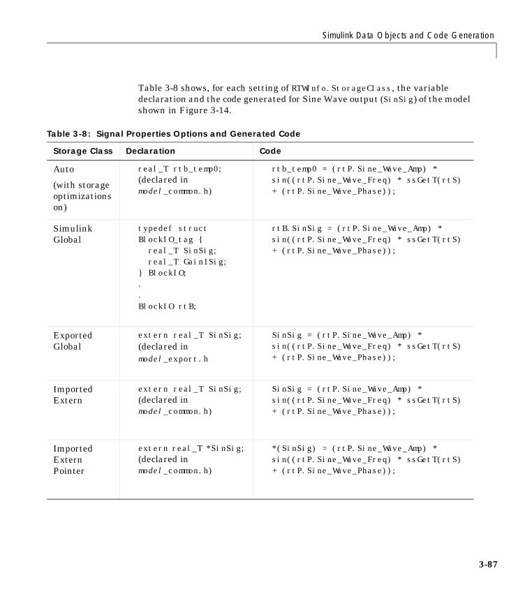
Simulink Data Objects and Code Generation
3-87
Table 3-8 shows, for each setting of RTWInfo.StorageClass, the variabledeclaration and the code generated for Sine Wave output (SinSig) of the modelshown in Figure 3-14.
Table 3-8: Signal Properties Options and Generated Code
Storage Class Declaration Code
Auto
(with storageoptimizationson)
real_T rtb_temp0;(declared inmodel_common.h)
rtb_temp0 = (rtP.Sine_Wave_Amp) * sin((rtP.Sine_Wave_Freq) * ssGetT(rtS) + (rtP.Sine_Wave_Phase));
SimulinkGlobal
typedef struct BlockIO_tag {real_T SinSig; real_T Gain1Sig;
} BlockIO;..BlockIO rtB;
rtB.SinSig = (rtP.Sine_Wave_Amp) * sin((rtP.Sine_Wave_Freq) * ssGetT(rtS) + (rtP.Sine_Wave_Phase));
ExportedGlobal
extern real_T SinSig;(declared inmodel_export.h
SinSig = (rtP.Sine_Wave_Amp) * sin((rtP.Sine_Wave_Freq) * ssGetT(rtS) + (rtP.Sine_Wave_Phase));
ImportedExtern
extern real_T SinSig;(declared inmodel_common.h)
SinSig = (rtP.Sine_Wave_Amp) * sin((rtP.Sine_Wave_Freq) * ssGetT(rtS) + (rtP.Sine_Wave_Phase));
ImportedExternPointer
extern real_T *SinSig;(declared inmodel_common.h)
*(SinSig) = (rtP.Sine_Wave_Amp) * sin((rtP.Sine_Wave_Freq) * ssGetT(rtS) + (rtP.Sine_Wave_Phase));
3 Code Generation and the Build Process
3-88
Object Property Information in the model.rtw FileDuring code generation, the Real-Time Workshop writes property informationabout signal and parameter objects to the model.rtw file. AnObjectProperties record is written for each parameter or signal that meetscertain conditions. These conditions are described in “ObjectProperties RecordsFor Parameters” on page 3-88 and “ObjectProperties Records For Signals” onpage 3-89.
The ObjectProperties records contain all of the property information from theassociated object. To access ObjectProperties records, you must write TargetLanguage Compiler code (see “Accessing Object Property Information via TLC”on page 3-90).
ObjectProperties Records For ParametersAn ObjectProperties record is included in the in the ModelParameters sectionof model.rtw file for each parameter, under the following conditions:
1 Inline parameters is on.
2 The parameter resolves to a Simulink.Parameter object (or to a parameterobject that comes from a class derived from the Simulink.Parameter class).
3 The parameter’s RTWInfo.StorageClass is set to anything but 'Auto'.
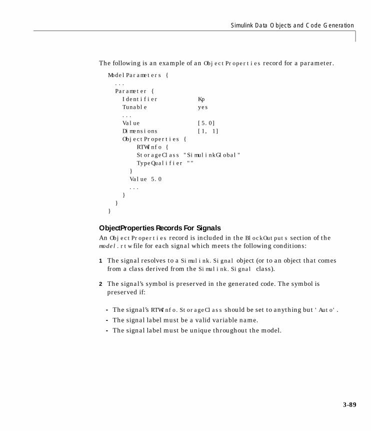
Simulink Data Objects and Code Generation
3-89
The following is an example of an ObjectProperties record for a parameter.
ModelParameters { ... Parameter { Identifier Kp Tunable yes ... Value [5.0] Dimensions [1, 1] ObjectProperties {
RTWInfo { StorageClass "SimulinkGlobal" TypeQualifier "" } Value 5.0 ... } }}
ObjectProperties Records For SignalsAn ObjectProperties record is included in the BlockOutputs section of themodel.rtw file for each signal which meets the following conditions:
1 The signal resolves to a Simulink.Signal object (or to an object that comesfrom a class derived from the Simulink.Signal class).
2 The signal’s symbol is preserved in the generated code. The symbol ispreserved if:
- The signal’s RTWInfo.StorageClass should be set to anything but 'Auto'.
- The signal label must be a valid variable name.
- The signal label must be unique throughout the model.
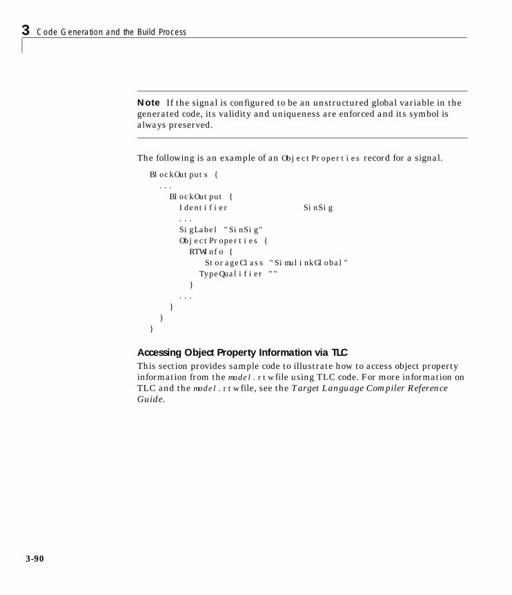
3 Code Generation and the Build Process
3-90
Note If the signal is configured to be an unstructured global variable in thegenerated code, its validity and uniqueness are enforced and its symbol isalways preserved.
The following is an example of an ObjectProperties record for a signal.
BlockOutputs { ... BlockOutput { Identifier SinSig ... SigLabel "SinSig" ObjectProperties { RTWInfo {
StorageClass "SimulinkGlobal" TypeQualifier "" } ... } }}
Accessing Object Property Information via TLCThis section provides sample code to illustrate how to access object propertyinformation from the model.rtw file using TLC code. For more information onTLC and the model.rtw file, see the Target Language Compiler ReferenceGuide.
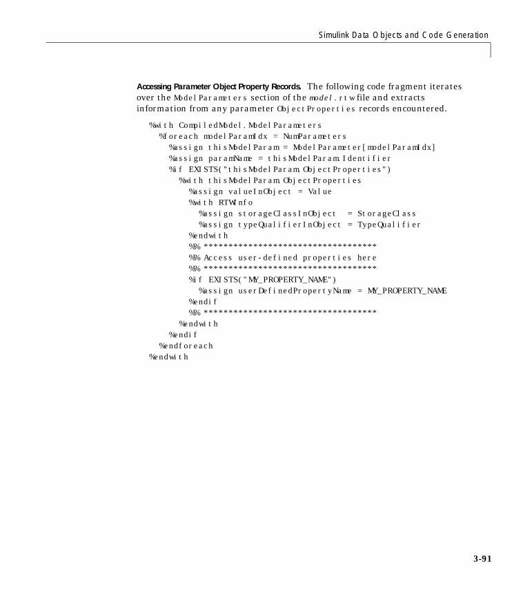
Simulink Data Objects and Code Generation
3-91
Accessing Parameter Object Property Records. The following code fragment iteratesover the ModelParameters section of the model.rtw file and extractsinformation from any parameter ObjectProperties records encountered.
%with CompiledModel.ModelParameters %foreach modelParamIdx = NumParameters %assign thisModelParam = ModelParameter[modelParamIdx] %assign paramName = thisModelParam.Identifier %if EXISTS("thisModelParam.ObjectProperties") %with thisModelParam.ObjectProperties %assign valueInObject = Value %with RTWInfo %assign storageClassInObject = StorageClass %assign typeQualifierInObject = TypeQualifier %endwith %% *********************************** %% Access user-defined properties here %% *********************************** %if EXISTS("MY_PROPERTY_NAME") %assign userDefinedPropertyName = MY_PROPERTY_NAME %endif %% *********************************** %endwith %endif %endforeach%endwith
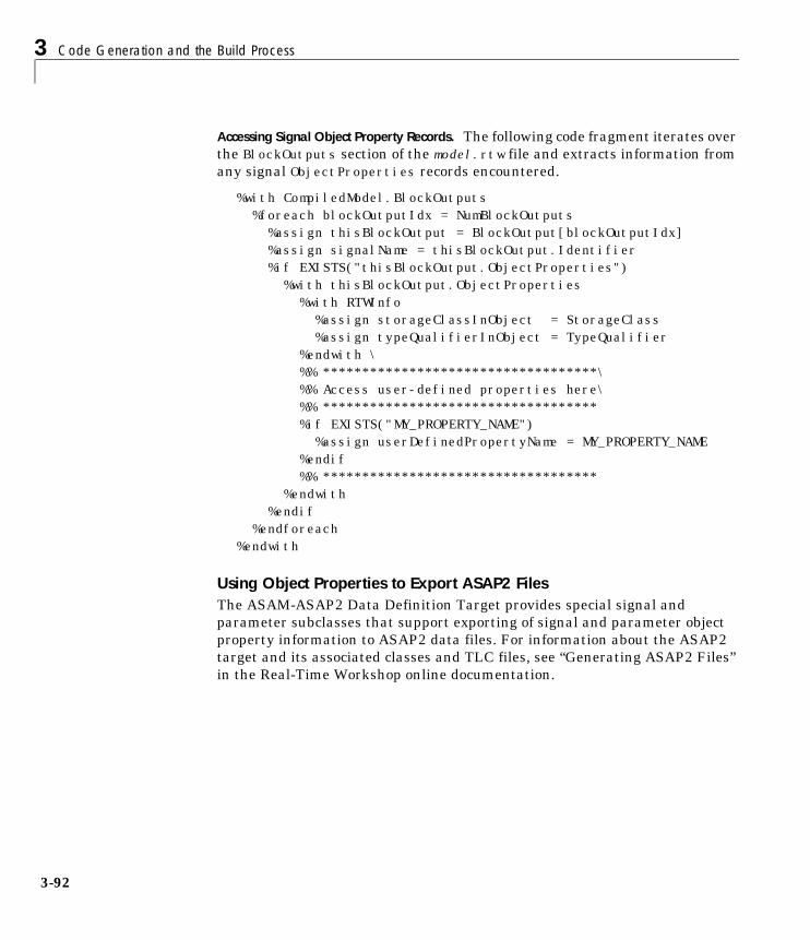
3 Code Generation and the Build Process
3-92
Accessing Signal Object Property Records. The following code fragment iterates overthe BlockOutputs section of the model.rtw file and extracts information fromany signal ObjectProperties records encountered.
%with CompiledModel.BlockOutputs %foreach blockOutputIdx = NumBlockOutputs %assign thisBlockOutput = BlockOutput[blockOutputIdx] %assign signalName = thisBlockOutput.Identifier %if EXISTS("thisBlockOutput.ObjectProperties") %with thisBlockOutput.ObjectProperties %with RTWInfo %assign storageClassInObject = StorageClass %assign typeQualifierInObject = TypeQualifier %endwith \ %% ***********************************\ %% Access user-defined properties here\ %% *********************************** %if EXISTS("MY_PROPERTY_NAME") %assign userDefinedPropertyName = MY_PROPERTY_NAME %endif %% *********************************** %endwith %endif %endforeach%endwith
Using Object Properties to Export ASAP2 Files The ASAM-ASAP2 Data Definition Target provides special signal andparameter subclasses that support exporting of signal and parameter objectproperty information to ASAP2 data files. For information about the ASAP2target and its associated classes and TLC files, see “Generating ASAP2 Files”in the Real-Time Workshop online documentation.

Configuring the Generated Code via TLC
3-93
Configuring the Generated Code via TLCThis section covers features of the Real-Time Workshop Target LanguageCompiler that help you to fine-tune your generated code. To learn more aboutTLC, read the Target Language Compiler Reference Guide.
Target Language Compiler Variables and OptionsThe Target Language Compiler supports extended code generation variablesand options in addition to those included in the code generation optionscategories of the Real-Time Workshop page.
There are two ways to set TLC variables and options:
• Assigning TLC variables in the system target file
• Entering TLC options or variables into the System Target File field on theReal-Time Workshop page
Assigning Target Language Compiler VariablesThe %assign statement lets you assign a value to a TLC variable, as in
%assign MaxStackSize = 4096
This is also known as creating a parameter name/parameter value pair.
The %assign statement is described in the Target Language CompilerReference Guide. It is recommended that you write your %assign statements inthe Configure RTW code generation settings section of the system targetfile.
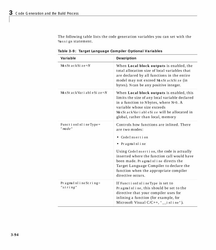
3 Code Generation and the Build Process
3-94
The following table lists the code generation variables you can set with the%assign statement.
Table 3-9: Target Language Compiler Optional Variables
Variable Description
MaxStackSize=N When Local block outputs is enabled, thetotal allocation size of local variables thatare declared by all functions in the entiremodel may not exceed MaxStackSize (inbytes). N can be any positive integer.
MaxStackVariableSize=N When Local block outputs is enabled, thislimits the size of any local variable declaredin a function to N bytes, where N>0. Avariable whose size exceedsMaxStackVariableSize will be allocated inglobal, rather than local, memory
FunctionInlineType="mode"
Controls how functions are inlined. Thereare two modes:
• CodeInsertion
• PragmaInline
Using CodeInsertion, the code is actuallyinserted where the function call would havebeen made. PragmaInline directs theTarget Language Compiler to declare thefunction when the appropriate compilerdirective occurs.
PragmaInlineString="string"
If FunctionInlineType is set toPragmaInline, this should be set to thedirective that your compiler uses forinlining a function (for example, forMicrosoft Visual C/C++, "__inline").
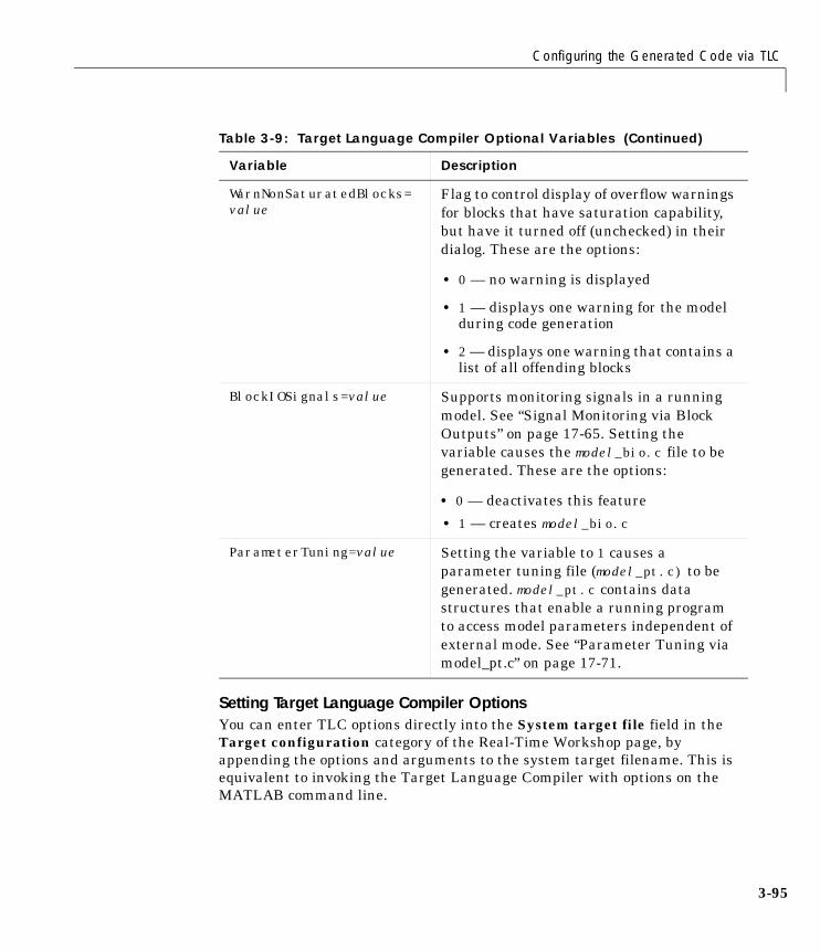
Configuring the Generated Code via TLC
3-95
Setting Target Language Compiler OptionsYou can enter TLC options directly into the System target file field in theTarget configuration category of the Real-Time Workshop page, byappending the options and arguments to the system target filename. This isequivalent to invoking the Target Language Compiler with options on theMATLAB command line.
WarnNonSaturatedBlocks= value
Flag to control display of overflow warningsfor blocks that have saturation capability,but have it turned off (unchecked) in theirdialog. These are the options:
• 0 — no warning is displayed
• 1 — displays one warning for the modelduring code generation
• 2 — displays one warning that contains alist of all offending blocks
BlockIOSignals=value Supports monitoring signals in a runningmodel. See “Signal Monitoring via BlockOutputs” on page 17-65. Setting thevariable causes the model_bio.c file to begenerated. These are the options:
• 0 — deactivates this feature
• 1 — creates model_bio.c
ParameterTuning=value Setting the variable to 1 causes aparameter tuning file (model_pt.c) to begenerated. model_pt.c contains datastructures that enable a running programto access model parameters independent ofexternal mode. See “Parameter Tuning viamodel_pt.c” on page 17-71.
Table 3-9: Target Language Compiler Optional Variables (Continued)
Variable Description
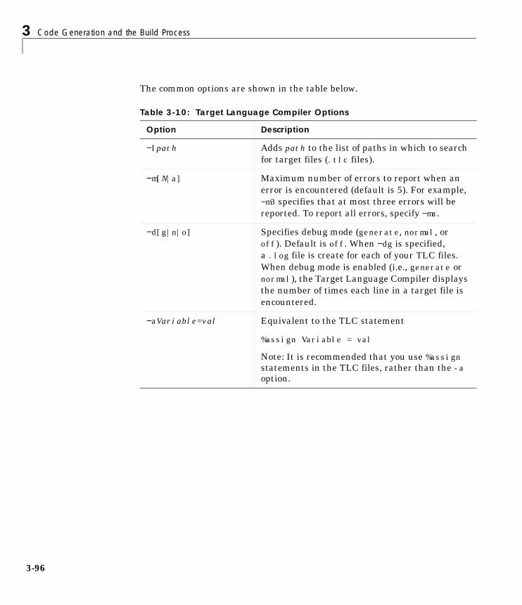
3 Code Generation and the Build Process
3-96
The common options are shown in the table below.
Table 3-10: Target Language Compiler Options
Option Description
−Ipath Adds path to the list of paths in which to searchfor target files (.tlc files).
−m[N|a] Maximum number of errors to report when anerror is encountered (default is 5). For example,−m3 specifies that at most three errors will bereported. To report all errors, specify −ma.
−d[g|n|o] Specifies debug mode (generate, normal, oroff). Default is off. When −dg is specified,a .log file is create for each of your TLC files.When debug mode is enabled (i.e., generate ornormal), the Target Language Compiler displaysthe number of times each line in a target file isencountered.
−aVariable=val Equivalent to the TLC statement
%assign Variable = val
Note: It is recommended that you use %assignstatements in the TLC files, rather than the -a option.
Making an Executable
3-97
Making an ExecutableAfter completing code generation, the build process determines whether or notto continue and compile and link an executable program. This decision isgoverned by the following parameters:
• Generate code only option
When this option is selected, the build process always omits the make phase.
• Makefile-only target
The Visual C/C++ Project Makefile versions of the grt, grt_malloc, andReal-Time Workshop Embedded Coder target configurations generate aVisual C/C++ project makefile (model.mak). To build an executable, you mustopen model.mak in the Visual C/C++ IDE and compile and link the modelcode.
• HOST template makefile variable
The template makefile variable HOST identifies the type of system uponwhich your executable is intended to run. The HOST variable can take on oneof three possible values: PC, UNIX, or ANY.
By default, HOST is set to UNIX in template makefiles designed for use withUNIX (such as grt_unix.tmf), and to PC in the template makefiles designedfor use with development systems for the PC (such as grt_vc.tmf).
If Simulink is running on the same type of system as that specified by theHOST variable, then the executable is built. Otherwise:
- If HOST = ANY, an executable is still built. This option is useful when youwant to cross-compile a program for a system other than the one Simulinkis running on.
- Otherwise, processing stops after generating the model code and themakefile; the following message is displayed on the MATLAB commandline.
### Make will not be invoked - template makefile is for a different host
3 Code Generation and the Build Process
3-98
Directories Used in the Build ProcessThe Real-Time Workshop creates output files in two directories during thebuild process:
• The working directory
If an executable is created, it is written to your working directory. Theexecutable is named model.exe (on PC) or model (on UNIX).
• The build directory
The build process creates a subdirectory, called the build directory, withinyour working directory. The build directory name is model_target_rtw,where model is the name of the source model and target is the name of thechosen target. The build directory stores generated source code and all otherfiles created during the build process (except the executable).
The build directory always contains the generated code modules model.c,model.h, and model_export.h, and the generated makefile model.mk.
Depending upon the target and code generation and build options selected,additional files in the build directory may include:
• model.rtw
• Object (.obj) files
• Code modules generated from subsystems
• TLC profiler report files
• Block I/O (model_bio.c) and parameter tuning (model_pt.c) informationfiles
• Real-Time Workshop project (model.tmw) files
Choosing and Configuring Your Compiler
3-99
Choosing and Configuring Your CompilerThe Real-Time Workshop build process depends upon the correct installationof one or more supported compilers. Note that compiler, in this context, refersto a development environment containing a linker and make utility, in additionto a high-level language compiler.
The build process also requires the selection of a template makefile. Thetemplate makefile determines which compiler will be run, during the makephase of the build, to compile the generated code.
This section discusses how to install a compiler and choose an appropriatetemplate makefile, on both Windows and UNIX systems.
Choosing and Configuring Your Compiler on WindowsOn Windows, you must install one or more supported compilers, In addition,you must define an environment variable associated with each compiler.Makesure that your compiler is installed as described in“Third-Party CompilerInstallation on Windows” on page -xxii.
You can select a template makefile that is specific to your compiler. Forexample, grt_bc.tmf designates the Borland C/C++ compiler, and grt_vc.tmf designates the Visual C/C++ compiler.
Alternatively, you can choose a default template makefile that will select thedefault compiler for your system. The default compiler is the compilerMATLAB uses to build MEX-files. You can set up the default compiler by usingthe MATLAB mex command as shown below.
mex –setup
See the MATLAB Application Program Interface Guide for information on themex command.
Default template makefiles are named target_default_tmf. For example, thedefault template makefile for the generic real-time (GRT) target isgrt_default_tmf.
The build process uses the following logic to locate a compiler for the generatedcode:
1 If a specific compiler is named in the template makefile, the build processuses that compiler.
3 Code Generation and the Build Process
3-100
2 If the template makefile designates a default compiler (as ingrt_default_tmf), the build process uses the same compiler as those usedfor building C MEX-files.
3 If no default compiler is established, the build process examinesenvironment variables which define the path to installed compilers, andselects the first compiler located. The variables are searched in the followingorder:
- MSDevDir or DEVSTUDIO (defining the path to the Microsoft Visual C/C++)
- WATCOM (defining the path to the Watcom C/C++ compiler)
- BORLAND (defining the path to the Borland C/C++ compiler)
4 If none of the above environment variables is defined, the build processselects the lcc compiler, which is shipped and installed with MATLAB.
Compile/Build Options for Visual C/C++. The Real-Time Workshop offers two sets oftemplate makefiles designed for use with Visual C/C++.
To compile under Visual C/C++ and build an executable within the Real-TimeWorkshop build process, use one of the target_vc.tmf template makefiles:
• ert_vc.tmf
• grt_malloc_vc.tmf
• grt_vc.tmf
• rsim_vc.tmf
Alternatively, you can choose to create a project makefile (model.mak) suitablefor use with the Visual C/C++ IDE. In this case, you must compile and link yourcode within the Visual C/C++ environment. To create a Visual C/C++ projectmakefile, choose one of the Visual C/C++ Project Makefile versions of the grt,ert, or grt_malloc target configurations. These configurations use thetarget_msvc.tmf template makefiles:
• ert_msvc.tmf
• grt_malloc_msvc.tmf
• grt_msvc.tmf
Choosing and Configuring Your Compiler
3-101
Choosing and Configuring Your Compiler On UNIXOn UNIX, the Real-Time Workshop build process uses the default compiler. ccis the default on all platforms except SunOS, where gcc is the default.
You should choose the UNIX-specific template makefile that is appropriate toyour target. For example, grt_unix.tmf is the correct template makefile tobuild a generic real-time program under UNIX.
Available Compiler/Makefile/Target ConfigurationsTo determine which template makefiles are appropriate for your compiler andtarget, see the table “Targets Available from the System Target File Browser”on page 3-36.

3 Code Generation and the Build Process
3-102
Template Makefiles and Make OptionsThe Real-Time Workshop includes a set of built-in template makefiles that aredesigned to build programs for specific targets.
There are two types of template makefiles:
• Compiler-specific template makefiles are designed for use with a particularcompiler or development system.
By convention, compiler-specific template makefiles are named according tothe target and compiler (or development system). For example, grt_vc.tmfis the template makefile for building a generic real-time program underVisual C/C++; ert_lcc.tmf is the template makefile for building aReal-Time Workshop Embedded Coder program under the LCC compiler.
• Default template makefiles make your model designs more portable, bychoosing the correct compiler-specific makefile and compiler for yourinstallation. “Choosing and Configuring Your Compiler” on page 3-99describes the operation of default template makefiles in detail.
Default template makefiles are named target_default_tmf. For example,grt_default_tmf is the default template makefile for building a genericreal-time program; ert_default_tmf is the default template makefilebuilding a Real-Time Workshop Embedded Coder program.
You can supply options to makefiles via arguments to the Make commandfield of the Target configuration category of the Real-Time Workshop page.Append the arguments after make_rtw (or make_xpc or other make command),as in the following example.
make_rtw OPTS="-DMYDEFINE=1"
The syntax for make command options differs slightly for different compilers.
Compiler-Specific Template MakefilesThis section documents the available compiler-specific template makefiles andcommon options you can use with each.
Template Makefiles for UNIX
• ert_unix.tmf
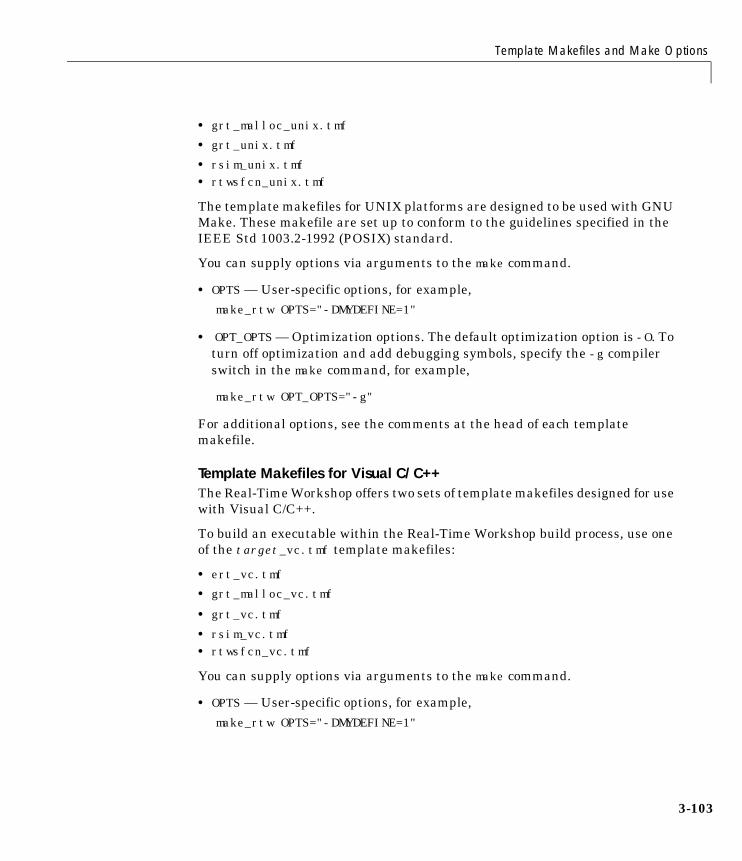
Template Makefiles and Make Options
3-103
• grt_malloc_unix.tmf
• grt_unix.tmf
• rsim_unix.tmf• rtwsfcn_unix.tmf
The template makefiles for UNIX platforms are designed to be used with GNUMake. These makefile are set up to conform to the guidelines specified in theIEEE Std 1003.2-1992 (POSIX) standard.
You can supply options via arguments to the make command.
• OPTS — User-specific options, for example,make_rtw OPTS="-DMYDEFINE=1"
• OPT_OPTS — Optimization options. The default optimization option is -O. Toturn off optimization and add debugging symbols, specify the -g compilerswitch in the make command, for example,
make_rtw OPT_OPTS="-g"
For additional options, see the comments at the head of each templatemakefile.
Template Makefiles for Visual C/C++The Real-Time Workshop offers two sets of template makefiles designed for usewith Visual C/C++.
To build an executable within the Real-Time Workshop build process, use oneof the target_vc.tmf template makefiles:
• ert_vc.tmf
• grt_malloc_vc.tmf
• grt_vc.tmf
• rsim_vc.tmf• rtwsfcn_vc.tmf
You can supply options via arguments to the make command.
• OPTS — User-specific options, for example,make_rtw OPTS="-DMYDEFINE=1"

3 Code Generation and the Build Process
3-104
• OPT_OPTS — Optimization options. The default optimization option is -Ot. Toturn off optimization and add debugging symbols, specify the -Zd compilerswitch in the make command.make_rtw OPT_OPTS="-Zd"
For additional options, see the comments at the head of each templatemakefile.
To create a Visual C/C++ project makefile (model.mak) without building anexecutable, use one of the target_msvc.tmf template makefiles:
• ert_msvc.tmf
• grt_malloc_msvc.tmf
• grt_msvc.tmf
These template makefiles are designed to be used with nmake, which is bundledwith Visual C/C++.
You can supply the following options via arguments to the nmake command:
• OPTS — User-specific options, for example,make_rtw OPTS="/D MYDEFINE=1"
For additional options, see the comments at the head of each templatemakefile.
Template Makefiles for Watcom C/C++
Note As of this printing, the Watcom C compiler is no longer available fromthe manufacturer. The Real-Time Workshop continues to ship Watcom-relatedtemplate makefiles at this time. However, this policy may be subject to changein the future.
• drt_watc.tmf
• ert_watc.tmf
• grt_malloc_watc.tmf
• grt_watc.tmf
• rsim_watc.tmf
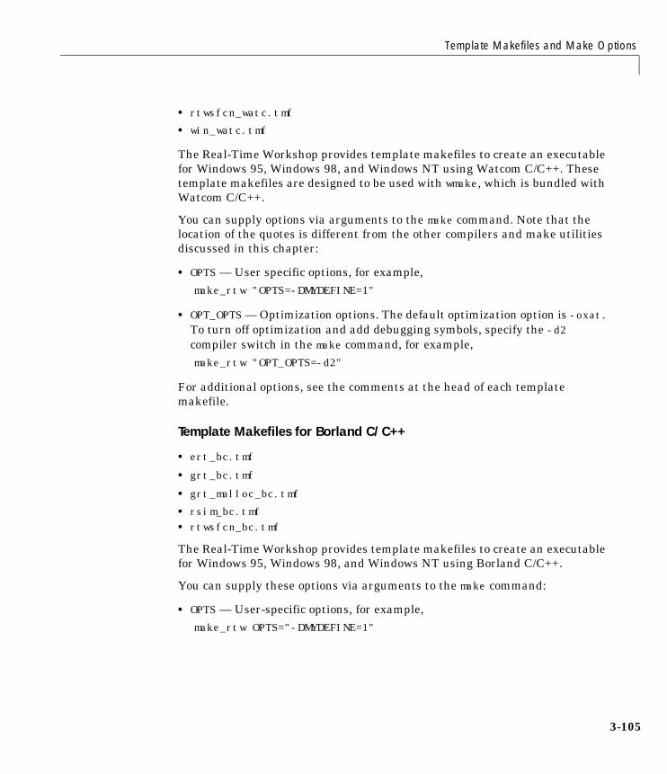
Template Makefiles and Make Options
3-105
• rtwsfcn_watc.tmf
• win_watc.tmf
The Real-Time Workshop provides template makefiles to create an executablefor Windows 95, Windows 98, and Windows NT using Watcom C/C++. Thesetemplate makefiles are designed to be used with wmake, which is bundled withWatcom C/C++.
You can supply options via arguments to the make command. Note that thelocation of the quotes is different from the other compilers and make utilitiesdiscussed in this chapter:
• OPTS — User specific options, for example,make_rtw "OPTS=-DMYDEFINE=1"
• OPT_OPTS — Optimization options. The default optimization option is -oxat.To turn off optimization and add debugging symbols, specify the -d2compiler switch in the make command, for example,make_rtw "OPT_OPTS=-d2"
For additional options, see the comments at the head of each templatemakefile.
Template Makefiles for Borland C/C++
• ert_bc.tmf
• grt_bc.tmf
• grt_malloc_bc.tmf
• rsim_bc.tmf• rtwsfcn_bc.tmf
The Real-Time Workshop provides template makefiles to create an executablefor Windows 95, Windows 98, and Windows NT using Borland C/C++.
You can supply these options via arguments to the make command:
• OPTS — User-specific options, for example,make_rtw OPTS="-DMYDEFINE=1"

3 Code Generation and the Build Process
3-106
• OPT_OPTS — Optimization options. Default is none. To turn off optimizationand add debugging symbols, specify the -v compiler switch in the makecommand.make_rtw OPT_OPTS="-v"
For additional options, see the comments at the head of each templatemakefile.
Template Makefiles for LCC
• ert_lcc.tmf
• grt_lcc.tmf
• grt_malloc_lcc.tmf• rsim_lcc.tmf• rtwsfcn_lcc.tmf
The Real-Time Workshop provides template makefiles to create an executablefor Windows 95, Windows 98, and Windows NT using LCC compiler Version2.4 and GNU Make (gmake).
You can supply options via arguments to the make command:
• OPTS — User-specific options, for example,make_rtw OPTS="-DMYDEFINE=1"
• OPT_OPTS — Optimization options. Default is none. To enable debugging,specify -g4 in the make command:make_rtw OPT_OPTS="-g4"
For additional options, see the comments at the head of each templatemakefile.
Template Makefile StructureThe detailed structure of template makefiles is documented in “TemplateMakefiles” on page 17-25. This information is provided for those who want tocustomize template makefiles.
4
Generated Code Formats
Introduction . . . . . . . . . . . . . . . . . . . . 4-2
Choosing a Code Format for Your Application . . . . . 4-3
Real-Time Code Format . . . . . . . . . . . . . . . 4-6Unsupported Blocks . . . . . . . . . . . . . . . . . 4-6System Target Files . . . . . . . . . . . . . . . . . 4-6Template Makefiles . . . . . . . . . . . . . . . . . . 4-6
Real-Time malloc Code Format . . . . . . . . . . . . 4-8Unsupported Blocks . . . . . . . . . . . . . . . . . 4-8System Target Files . . . . . . . . . . . . . . . . . 4-8Template Makefiles . . . . . . . . . . . . . . . . . . 4-8
S-Function Code Format . . . . . . . . . . . . . . . 4-10
Embedded C Code Format . . . . . . . . . . . . . . 4-11
4 Generated Code Formats
4-2
IntroductionThe Real-Time Workshop provides five different code formats. Each codeformat specifies a framework for code generation suited for specificapplications.
The five code formats and corresponding application areas are:
• Real-time: Rapid prototyping
• Real-time malloc: Rapid prototyping
• S-function: Creating proprietary S-function .dll or MEX-file objects, codereuse, and speeding up your simulation
• Embedded C: Deeply embedded systems
• Ada
Note Generation of Ada code requires the Real-Time Workshop Ada Coder, aseparate product. See Chapter 16, “Real-Time Workshop Ada Coder” for moreinformation.
This chapter discusses the relationship of code formats to the available targetconfigurations, and factors you should consider when choosing a code formatand target. This chapter also summarizes the real-time, real-time malloc,S-function, and embedded C code formats.
Choosing a Code Format for Your Application
4-3
Choosing a Code Format for Your ApplicationYour choice of code format is the most important code generation option. Thecode format specifies the overall framework of the generated code anddetermines its style.
When you choose a target, you implicitly choose a code format. Typically, thesystem target file will specify the code format by assigning the TLC variableCodeFormat. The following example is from ert.tlc.
%assign CodeFormat = "Embedded-C"
If the system target file does not assign CodeFormat, the default is RealTime (asin grt.tlc).
If you are developing a custom target, you must consider which code format isbest for your application and assign CodeFormat accordingly.
Choose the real-time or real-time malloc code format for rapid prototyping. Ifyour application does not have significant restrictions in code size, memoryusage, or stack usage, you may want to continue using the generic real-time(GRT) target throughout development. The real-time format is the mostcomprehensive code format and supports almost all the built-in blocks.
If your application demands that you limit source code size, memory usage, ormaintain a simple call structure, then you should choose the Real-TimeWorkshop Embedded Coder target, which uses the embedded C format.
Finally, you should choose the S-function format if you are not concerned aboutRAM and ROM usage and want to:
• Use a model as a component, for scalability
• Create a proprietary S-function .dll or MEX-file object
• Interface the generated code using the S-function C API
• Speed up your simulation
Table 4-1 summarizes the various options available for each code format/targetavailable in the Real-Time Workshop.
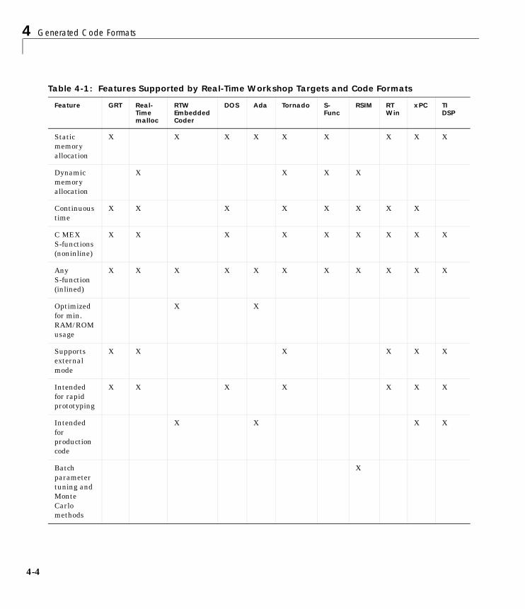
4 Generated Code Formats
4-4
Table 4-1: Features Supported by Real-Time Workshop Targets and Code Formats
Feature GRT Real-Time malloc
RTW Embedded Coder
DOS Ada Tornado S-Func
RSIM RTWin
xPC TIDSP
Staticmemoryallocation
X X X X X X X X X
Dynamicmemoryallocation
X X X X
Continuoustime
X X X X X X X X
C MEXS-functions(noninline)
X X X X X X X X X
AnyS-function(inlined)
X X X X X X X X X X X
Optimizedfor min.RAM/ ROMusage
X X
Supportsexternalmode
X X X X X X
Intendedfor rapidprototyping
X X X X X X X
Intendedforproductioncode
X X X X
Batchparametertuning andMonteCarlomethods
X
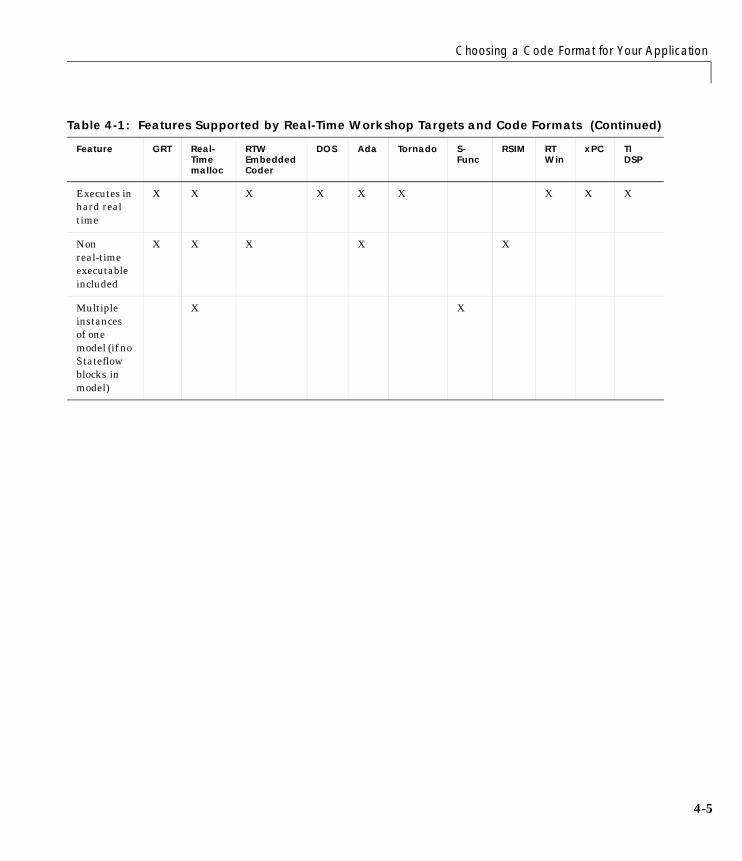
Choosing a Code Format for Your Application
4-5
Executes inhard realtime
X X X X X X X X X
Nonreal-timeexecutableincluded
X X X X X
Multipleinstancesof onemodel (if noStateflowblocks inmodel)
X X
Table 4-1: Features Supported by Real-Time Workshop Targets and Code Formats (Continued)
Feature GRT Real-Time malloc
RTW Embedded Coder
DOS Ada Tornado S-Func
RSIM RTWin
xPC TIDSP
4 Generated Code Formats
4-6
Real-Time Code FormatThe real-time code format (corresponding to the generic real-time target) isuseful for rapid prototyping applications. If you want to generate real-timecode while iterating model parameters rapidly, you should begin the designprocess with the generic real-time target. The real-time code format supports:
• Continuous time
• Continuous states
• C MEX S-functions (inlined and noninlined)
For more information on inlining S-functions, see the Target LanguageCompiler Reference Guide.
The real-time code format declares memory statically, that is, at compile time.
Unsupported BlocksThe real-time format does not support the following built-in blocks:
• Functions & Tables
- MATLAB Fcn
- S-Function — M-file and Fortran S-functions, C MEX S-functions that callinto MATLAB.
System Target Files• drt.tlc — DOS real-time target• grt.tlc — generic real-time target
• osek_leo.tlc — Lynx-Embedded OSEK target
• rsim.tlc — rapid simulation target
• tornado.tlc — Tornado (VxWorks) real-time target
Template Makefiles• drt.tmf
• grt
- grt_bc.tmf — Borland C
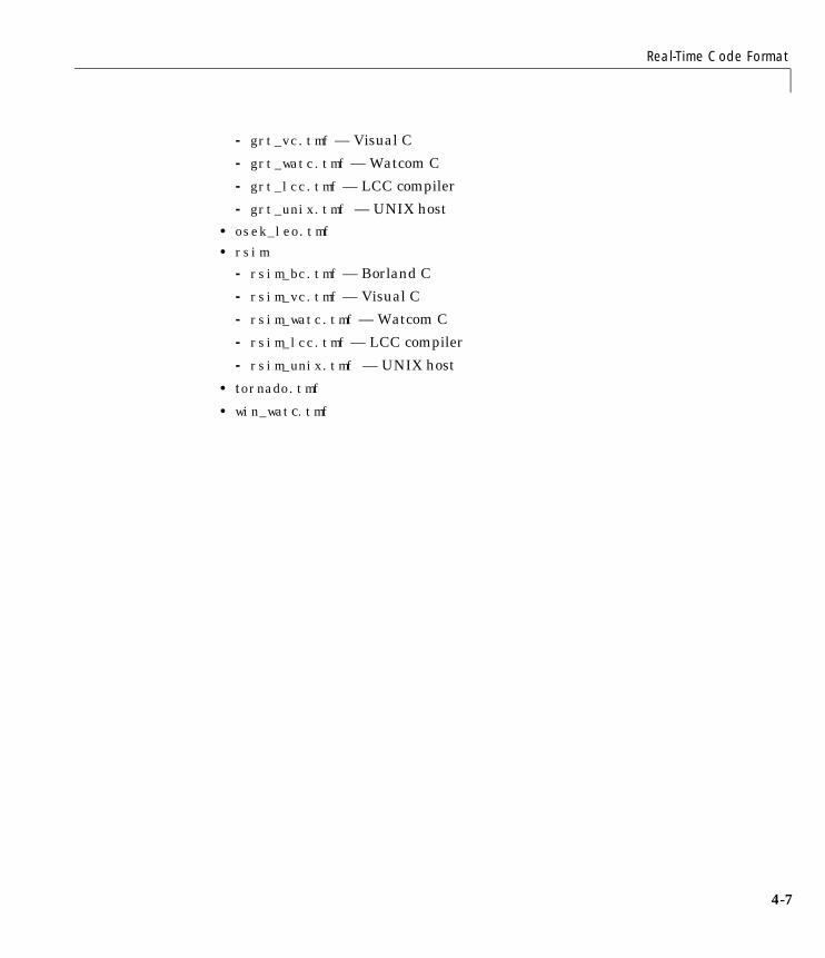
Real-Time Code Format
4-7
- grt_vc.tmf — Visual C
- grt_watc.tmf — Watcom C
- grt_lcc.tmf — LCC compiler
- grt_unix.tmf — UNIX host• osek_leo.tmf
• rsim
- rsim_bc.tmf — Borland C
- rsim_vc.tmf — Visual C
- rsim_watc.tmf — Watcom C
- rsim_lcc.tmf — LCC compiler
- rsim_unix.tmf — UNIX host
• tornado.tmf
• win_watc.tmf

4 Generated Code Formats
4-8
Real-Time malloc Code FormatThe real-time malloc code format (corresponding to the generic real-timemalloc target) is very similar to the real-time code format. The differences are:
• Real-time malloc declares memory dynamically.
• Real-time malloc allows you to multiply instance the same model with eachinstance maintaining its own unique data.
• Real-time malloc allows you to combine multiple models together in oneexecutable. For example, to integrate two models into one larger executable,real-time malloc maintains a unique instance of each of the two models. Ifyou do not use the real-time malloc format, the Real-Time Workshop will notnecessarily create uniquely named data structures for each model,potentially resulting in name clashes.
grt_malloc_main.c, the main routine for the generic real-time malloc(grt_malloc) target, supports one model by default. See“CombiningMultiple Models” on page 17–82 for information on modifyinggrt_malloc_main to support multiple models. grt_malloc_main.c is locatedin the directory matlabroot/rtw/c/grt_malloc.
Unsupported BlocksThe real-time malloc format does not support the following built-in blocks:
• Functions & Tables
- MATLAB Fcn
- S-Function — M-file and Fortran S-functions, C MEX S-functions that callinto MATLAB.
System Target Files• grt_malloc.tlc
• tornado.tlc — Tornado (VxWorks) real-time target
Template Makefiles• grt_malloc
- grt_malloc_bc.tmf — Borland C
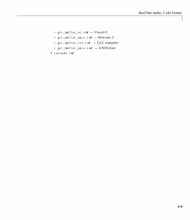
Real-Time malloc Code Format
4-9
- grt_malloc_vc.tmf — Visual C
- grt_malloc_watc.tmf — Watcom C
- grt_malloc_lcc.tmf — LCC compiler
- grt_malloc_unix.tmf — UNIX host• tornado.tmf

4 Generated Code Formats
4-10
S-Function Code FormatThe S-function code format (corresponding to the S-Function Target) generatescode that conforms to the Simulink C MEX S-function API. Using theS-Function Target, you can build an S-function component and use it as anS-Function block in another model.
The S-function code format is also used by the Simulink Accelerator to createthe Accelerator MEX-file.
In general you should not use the S-function code format in a system target file.However, you may need to do special handling in your inlined TLC files toaccount for this format. You can check the TLC variable CodeFormat to see ifthe current target is a MEX-file. If CodeFormat = "S-Function” and the TLCvariable Accelerator is set to 1, the target is a Simulink Accelerator MEX-file.
See Chapter 10, “The S-Function Target” for further information.
Embedded C Code Format
4-11
Embedded C Code FormatThe embedded C code format corresponds to the Real-Time WorkshopEmbedded Coder target. This code format includes a number of memory-savingand performance optimizations. See Chapter 9, “Real-Time WorkshopEmbedded Coder” for full details.

4 Generated Code Formats
4-12
5
External Mode
Introduction . . . . . . . . . . . . . . . . . . . . 5-2
Tutorial: Getting Started with External Mode Using GRT . 5-4Part 1: Setting Up the Model . . . . . . . . . . . . . . 5-4Part 2: Building the Target Executable . . . . . . . . . . 5-6Part 3: Running the External Mode Target Program . . . . 5-11Part 4: Tuning Parameters . . . . . . . . . . . . . . . 5-14
Using the External Mode User Interface . . . . . . . . 5-16External Mode Related Menu and Toolbar Items . . . . . . 5-16External Mode Control Panel . . . . . . . . . . . . . . 5-21Connection and Start/Stop Controls . . . . . . . . . . . 5-22Target Interface Dialog Box . . . . . . . . . . . . . . 5-23External Signal & Triggering Dialog Box . . . . . . . . . 5-24Data Archiving . . . . . . . . . . . . . . . . . . . 5-28Parameter Download Options . . . . . . . . . . . . . 5-31
External Mode Compatible Blocks and Subsystems . . . 5-32Compatible Blocks . . . . . . . . . . . . . . . . . . 5-32Signal Viewing Subsystems . . . . . . . . . . . . . . 5-32
Overview of External Mode Communications . . . . . . 5-36The Download Mechanism . . . . . . . . . . . . . . . 5-36
The TCP/IP Implementation . . . . . . . . . . . . . 5-38Overview . . . . . . . . . . . . . . . . . . . . . . 5-38Using the TCP/IP Implementation . . . . . . . . . . . 5-38The External Interface MEX-File . . . . . . . . . . . . 5-40External Mode Compatible Targets . . . . . . . . . . . 5-41Running the External Program . . . . . . . . . . . . . 5-41Error Conditions . . . . . . . . . . . . . . . . . . . 5-44Implementing an External Mode Protocol Layer . . . . . . 5-44
Limitations of External Mode . . . . . . . . . . . . . 5-45
5 External Mode
5-2
IntroductionExternal mode allows two separate systems — a host and a target — tocommunicate. The host is the computer where MATLAB and Simulink areexecuting. The target is the computer where the executable created by theReal-Time Workshop runs.
The host (Simulink) transmits messages requesting the target to acceptparameter changes or to upload signal data. The target responds by executingthe request. External mode communication is based on a client/serverarchitecture, in which Simulink is the client and the target is the server.
External mode lets you:
• Modify, or tune, block parameters in real time. In external mode, wheneveryou change parameters in the block diagram, Simulink automaticallydownloads them to the executing target program. This lets you tune yourprogram’s parameters without recompiling. In external mode, the Simulinkmodel becomes a graphical front end to the target program.
• View and log block outputs in many types of blocks and subsystems. You canmonitor and/or store signal data from the executing target program, withoutwriting special interface code. You can define the conditions under whichdata is uploaded from target to host. For example, data uploading could betriggered by a selected signal crossing zero in a positive direction.Alternatively, you can manually trigger data uploading.
External mode works by establishing a communication channel betweenSimulink and the Real-Time Workshop generated code. This channel isimplemented by a low-level transport layer that handles physical transmissionof messages. Both Simulink and the generated model code are independent ofthis layer. The transport layer and the code directly interfacing to the transportlayer are isolated in separate modules that format, transmit, and receivemessages and data packets.
This design makes it possible for different targets to use different transportlayers. For example, the GRT, GRT malloc, and Tornado targets support host/target communication via TCP/IP, whereas the xPC Target supports bothRS232 (serial) and TCP/IP communication. The Real-Time Windows Targetimplements external mode communication via shared memory.

5-3
This chapter discusses the following topics:
• “Tutorial: Getting Started with External Mode Using GRT” on page 5–4covers the basics of how to use external mode on a single computer.
• “Using the External Mode User Interface” on page 5–16 covers all elementsof the external mode user interface in detail.
• “External Mode Compatible Blocks and Subsystems” on page 5–32 discussesthe types of blocks that you can use to receive and view signals in externalmode.
• “Signal Viewing Subsystems” on page 5-32 shows how you can usesubsystems to encapsulate processing and viewing of signals received fromthe target system. This feature can help you generate a smaller and moreefficient target program.
• “Overview of External Mode Communications” on page 5-36 summarizes thecommunications process between Simulink and the target program.
• “The TCP/IP Implementation” on page 5-38 discusses the TCP/IP-basedimplementation of the external mode protocol that is provided by theReal-Time Workshop. This section includes information on bundled targetsthat support this implementation, and on how to build and run targetprograms that support the TCP/IP implementation.
• “Limitations of External Mode” on page 5-45 discusses limitations on the useof external mode that are imposed by the structure of the model.
Additional Reading“Creating an External Mode Communication Channel” on page 17–73 containsadvanced information for those who want to implement their own externalmode communications layer. You may want to read it for additional insight intothe architecture and code structure of external mode communications.
Chapter 12, “Targeting Tornado for Real-Time Applications” discusses the useof external mode in the VxWorks Tornado environment.
5 External Mode
5-4
Tutorial: Getting Started with External Mode Using GRTThis section provides step-by-step instructions for getting started withexternal mode. This tutorial assumes you have basic familiarity with MATLABand Simulink. In addition, you should read Chapter 1, “Introduction to theReal-Time Workshop.” Read “Getting Started: Basic Concepts and Tutorials”on page 1-37 and do the “Quick Start Tutorials” on page 1-40 before proceeding.
The example presented uses the generic real-time (GRT) target. The exampledoes not require any hardware other than the computer on which you runSimulink and the Real-Time Workshop. The generated executable in thisexample runs on the host computer under a separate process from MATLABand Simulink. This technique is called self-targeting.
The procedures for building, running, and testing your programs are almostidentical in UNIX and PC environments. The discussion notes differenceswhere applicable.
For a more thorough description of external mode, including a discussion of allthe options available, see “Using the External Mode User Interface” on page5-16.
Part 1: Setting Up the ModelIn this part of the tutorial, you create a simple model, ext_example, and adirectory called ext_mode_example to store the model and the generatedexecutable:
1 Create the directory from the MATLAB command line by typing
mkdir ext_mode_example
2 Make ext_mode_example your working directory.
cd ext_mode_example
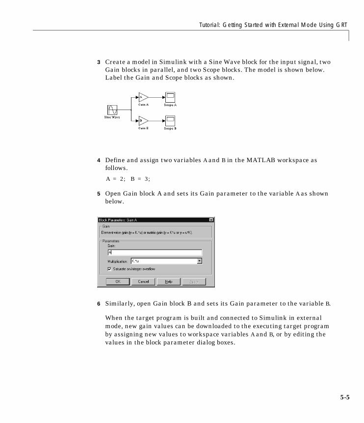
Tutorial: Getting Started with External Mode Using GRT
5-5
3 Create a model in Simulink with a Sine Wave block for the input signal, twoGain blocks in parallel, and two Scope blocks. The model is shown below.Label the Gain and Scope blocks as shown.
4 Define and assign two variables A and B in the MATLAB workspace asfollows.
A = 2; B = 3;
5 Open Gain block A and sets its Gain parameter to the variable A as shownbelow.
6 Similarly, open Gain block B and sets its Gain parameter to the variable B.
When the target program is built and connected to Simulink in externalmode, new gain values can be downloaded to the executing target programby assigning new values to workspace variables A and B, or by editing thevalues in the block parameter dialog boxes.

5 External Mode
5-6
7 Verify correct operation of the model. Open the Scope blocks and run themodel. Given that A=2 and B=3, the output should look like this.
8 From the File menu, choose Save As. Save the model as ext_example.mdl.
Part 2: Building the Target ExecutableIn this section, you set up the model and code generation parameters requiredfor an external mode compatible target program. Then you generate code andbuild the target executable.
9 Open the Simulation Parameters dialog box. On the Solver page, set theSolver options Type to Fixed-step, and the algorithm to discrete (no continuous states). Set Fixed-step Size to 0.01. Leave the otherparameters at their default values.
10 On the Workspace I/O page, deselect Time and Output. In this exercise,data will not be logged to the workspace or to a MAT-file.
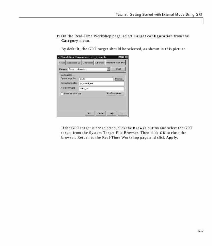
Tutorial: Getting Started with External Mode Using GRT
5-7
11 On the Real-Time Workshop page, select Target configuration from theCategory menu.
By default, the GRT target should be selected, as shown in this picture.
If the GRT target is not selected, click the Browse button and select the GRTtarget from the System Target File Browser. Then click OK to close thebrowser. Return to the Real-Time Workshop page and click Apply.
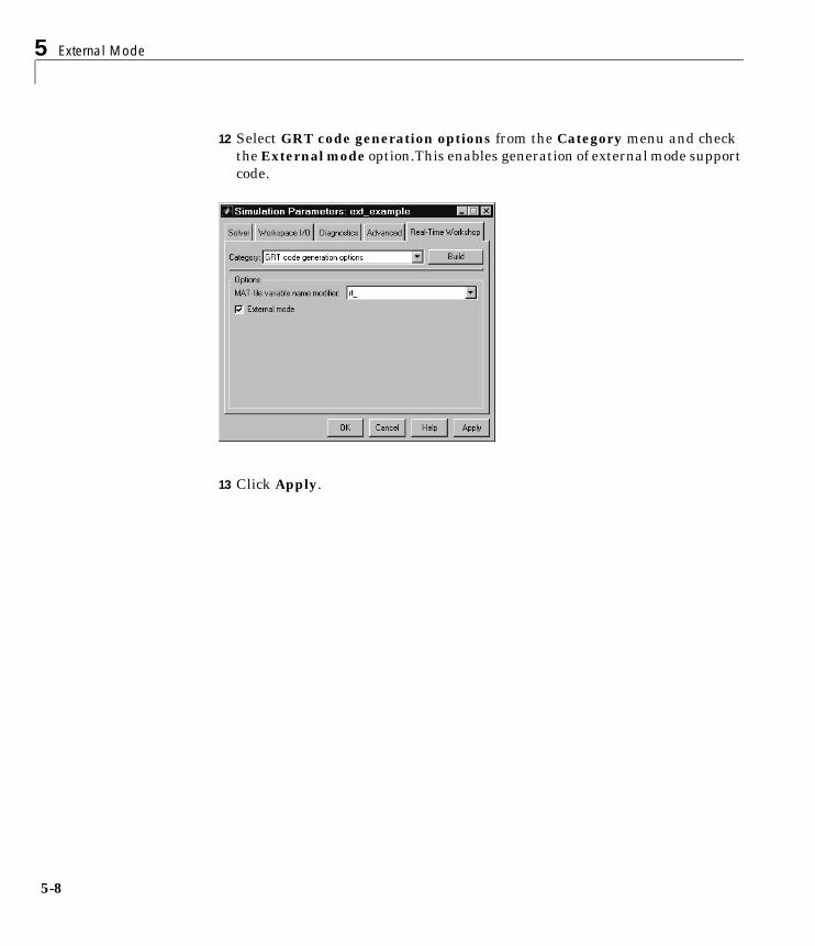
5 External Mode
5-8
12 Select GRT code generation options from the Category menu and checkthe External mode option.This enables generation of external mode supportcode.
13 Click Apply.
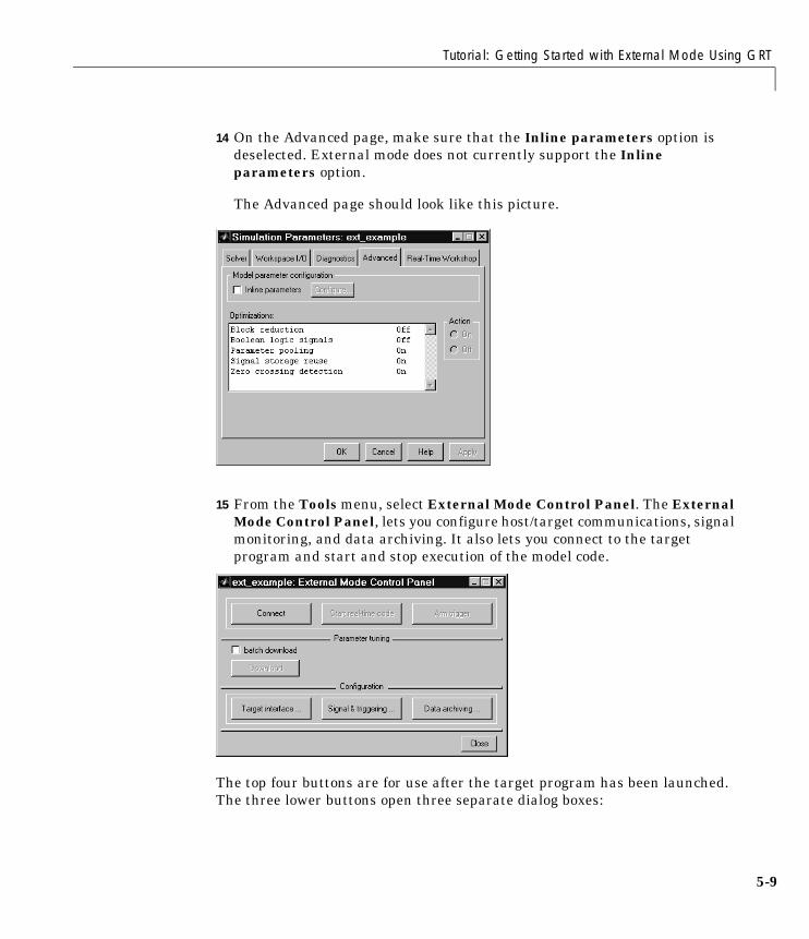
Tutorial: Getting Started with External Mode Using GRT
5-9
14 On the Advanced page, make sure that the Inline parameters option isdeselected. External mode does not currently support the Inlineparameters option.
The Advanced page should look like this picture.
15 From the Tools menu, select External Mode Control Panel. The ExternalMode Control Panel, lets you configure host/target communications, signalmonitoring, and data archiving. It also lets you connect to the targetprogram and start and stop execution of the model code.
The top four buttons are for use after the target program has been launched.The three lower buttons open three separate dialog boxes:
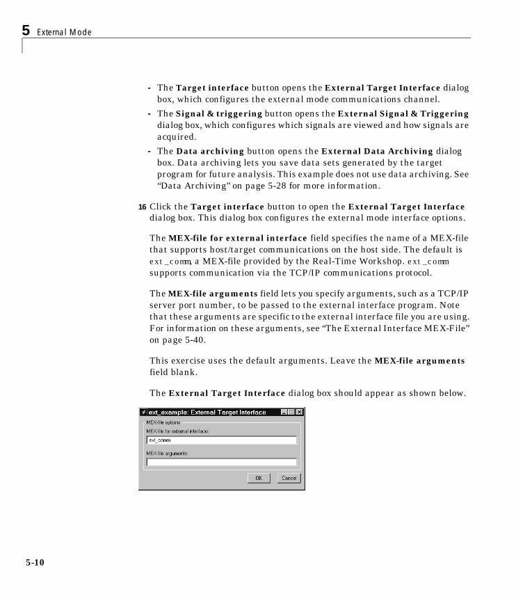
5 External Mode
5-10
- The Target interface button opens the External Target Interface dialogbox, which configures the external mode communications channel.
- The Signal & triggering button opens the External Signal & Triggeringdialog box, which configures which signals are viewed and how signals areacquired.
- The Data archiving button opens the External Data Archiving dialogbox. Data archiving lets you save data sets generated by the targetprogram for future analysis. This example does not use data archiving. See“Data Archiving” on page 5-28 for more information.
16 Click the Target interface button to open the External Target Interfacedialog box. This dialog box configures the external mode interface options.
The MEX-file for external interface field specifies the name of a MEX-filethat supports host/target communications on the host side. The default isext_comm, a MEX-file provided by the Real-Time Workshop. ext_commsupports communication via the TCP/IP communications protocol.
The MEX-file arguments field lets you specify arguments, such as a TCP/IPserver port number, to be passed to the external interface program. Notethat these arguments are specific to the external interface file you are using.For information on these arguments, see “The External Interface MEX-File”on page 5-40.
This exercise uses the default arguments. Leave the MEX-file argumentsfield blank.
The External Target Interface dialog box should appear as shown below.
Tutorial: Getting Started with External Mode Using GRT
5-11
17 Click OK to close the External Target Interface dialog box and return tothe External Mode Control Panel.
18 Close the External Mode Control Panel.
19 Save the model.
20 Return to the Real-Time Workshop page. Click Build to generate code andcreate the target program. The content of the succeeding messages dependson your compiler and operating system.The final message is
### Successful completion of Real-Time Workshop build procedure for model: ext_example
In the next section, you will run the ext_example executable and use Simulinkas an interactive front end to the running target program.
Part 3: Running the External Mode Target ProgramThe target executable, ext_example, is now in your working directory. In thissection, you run the target program and establish communication betweenSimulink and the target.
The External Signal & Triggering dialog box displays a list of all the blocksin your model that support external mode signal monitoring and logging. TheExternal Signal & Triggering dialog box also lets you configure which signalsare viewed and how they are acquired and displayed. You can reconfigure theExternal Signal & Triggering dialog box while the target program runs.
In this exercise you will observe and use the default settings of the ExternalSignal & Triggering dialog box.
21 From the Tools menu, select External Mode Control Panel.
22 In the External Mode Control Panel, click the Signal & triggering button.
23 The External Signal & Triggering dialog box opens. The defaultconfiguration of the External Signal & Triggering dialog box is designed toensure that all signals are selected for monitoring. The default configurationalso ensures that signal monitoring will begin as soon as the host and target
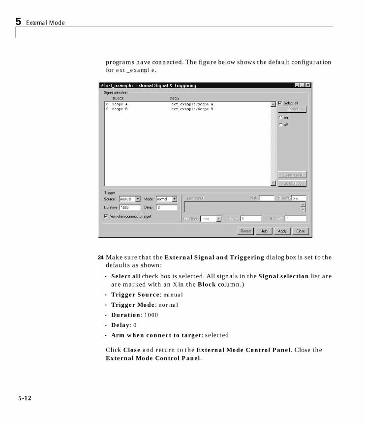
5 External Mode
5-12
programs have connected. The figure below shows the default configurationfor ext_example.
24 Make sure that the External Signal and Triggering dialog box is set to thedefaults as shown:
- Select all check box is selected. All signals in the Signal selection list areare marked with an X in the Block column.)
- Trigger Source: manual
- Trigger Mode: normal
- Duration: 1000
- Delay: 0
- Arm when connect to target: selected
Click Close and return to the External Mode Control Panel. Close theExternal Mode Control Panel.
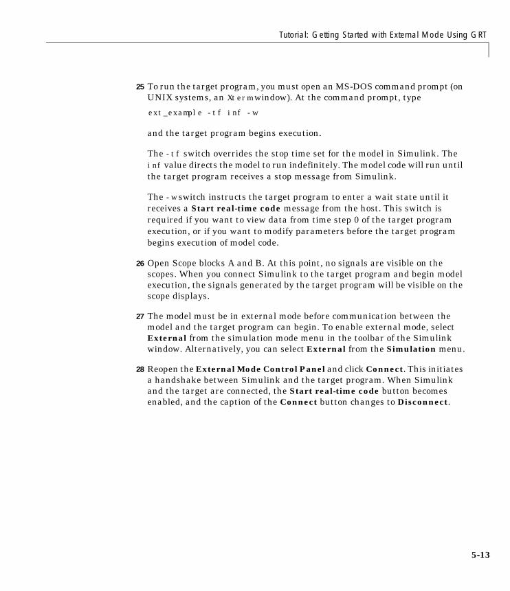
Tutorial: Getting Started with External Mode Using GRT
5-13
25 To run the target program, you must open an MS-DOS command prompt (onUNIX systems, an Xterm window). At the command prompt, type
ext_example -tf inf -w
and the target program begins execution.
The -tf switch overrides the stop time set for the model in Simulink. Theinf value directs the model to run indefinitely. The model code will run untilthe target program receives a stop message from Simulink.
The -w switch instructs the target program to enter a wait state until itreceives a Start real-time code message from the host. This switch isrequired if you want to view data from time step 0 of the target programexecution, or if you want to modify parameters before the target programbegins execution of model code.
26 Open Scope blocks A and B. At this point, no signals are visible on thescopes. When you connect Simulink to the target program and begin modelexecution, the signals generated by the target program will be visible on thescope displays.
27 The model must be in external mode before communication between themodel and the target program can begin. To enable external mode, selectExternal from the simulation mode menu in the toolbar of the Simulinkwindow. Alternatively, you can select External from the Simulation menu.
28 Reopen the External Mode Control Panel and click Connect. This initiatesa handshake between Simulink and the target program. When Simulinkand the target are connected, the Start real-time code button becomesenabled, and the caption of the Connect button changes to Disconnect.
5 External Mode
5-14
29 Click the Start real-time code button.You should see the outputs of Gainblocks A and B on the two scopes in your model. With A=2 and B=3, theoutput looks like this.
Having established communication between Simulink and the running targetprogram, you can tune block parameters in Simulink and observe the effectsthe parameter changes have on the target program. You will do this in the nextsection.
Part 4: Tuning ParametersYou can change the gain factor of either Gain block by assigning new values tothe variables A or B in the MATLAB workspace. When you change blockparameter values in the workspace during a simulation, you must explicitlyupdate the block diagram with these changes. When the block diagram isupdated, the new values are downloaded to the target program. To tune thevariables A and B:
30 In the MATLAB command window, assign new values to both variables, forexample
A = 0.5;B = 3.5;
31 Activate the ext_example model window. Select Update Diagram from theEdit menu, or type Ctrl+D. As soon as Simulink has updated the blockparameters, the new gain values are downloaded to the target program, andthe effect of the gain change becomes visible on the scopes.
Tutorial: Getting Started with External Mode Using GRT
5-15
You can also enter gain values directly into the Gain blocks. To do this:
32 Open the dialog box for Gain block A or B in the model.
33 Enter a new numerical value for the gain and click Apply. As soon as youclick Apply, the new value is downloaded to the target program and theeffect of the gain change becomes visible on the scope.
Similarly, you can change the frequency, amplitude, or phase of the sinewave signal by opening the dialog box for the Sine Wave block and enteringa new numerical value in the appropriate field.
Note, however, that you cannot change the sample time of the Sine Waveblock. Block sample times are part of the structural definition of the modeland are part of the generated code. Therefore, if you want to change a blocksample time, you must stop the external mode simulation and rebuild theexecutable.
34 To simultaneously disconnect host/target communication and end executionof the target program, pull down the Simulation menu and select Stopreal-time code.

5 External Mode
5-16
Using the External Mode User InterfaceThis section discusses the elements of the Simulink and Real-Time Workshopuser interface that control the operation of external mode. These elementsinclude:
• External mode related menu items in Simulation and Tools menus and inthe Simulink toolbar.
• External Mode Control Panel
• External Target Interface dialog box
• External Signal & Triggering dialog box
• External Data Archiving dialog box
External Mode Related Menu and Toolbar ItemsTo communicate with a target program, the model must be operating inexternal mode. The Simulation menu and the toolbar provide two ways toenable external mode:
• Select External from the Simulation menu.
• Select External from the simulation mode menu in the toolbar. Thesimulation mode menu is shown in this picture.
Once external mode is enabled, you can use the Simulation menu or thetoolbar to connect to and control the target program.
Simulation modemenu
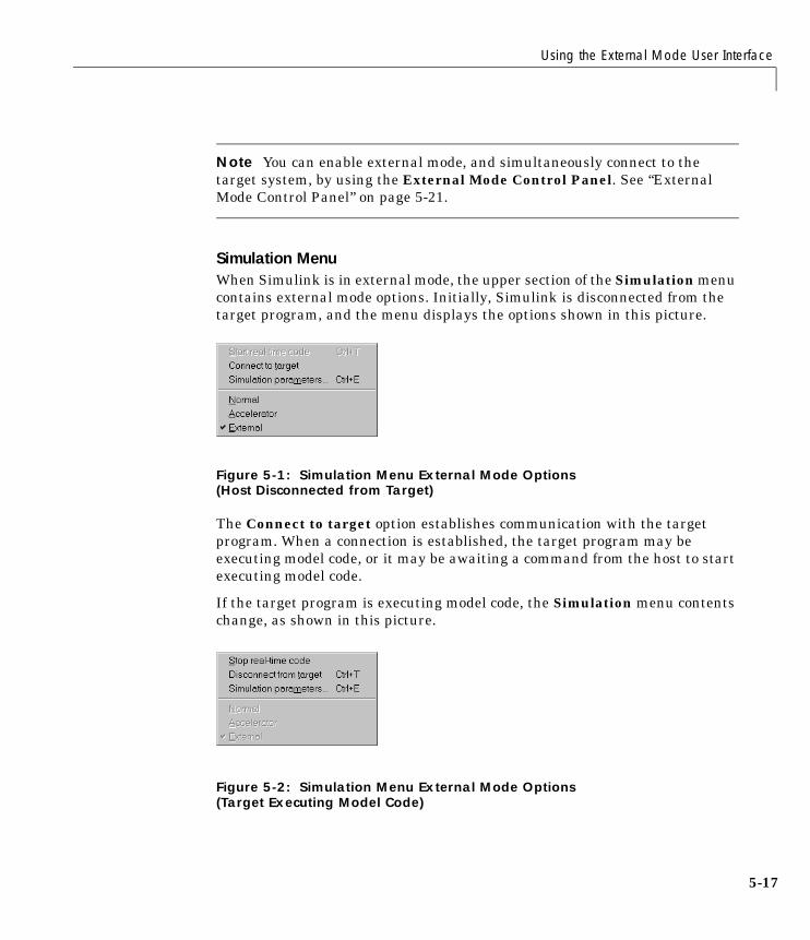
Using the External Mode User Interface
5-17
Note You can enable external mode, and simultaneously connect to thetarget system, by using the External Mode Control Panel. See “ExternalMode Control Panel” on page 5-21.
Simulation MenuWhen Simulink is in external mode, the upper section of the Simulation menucontains external mode options. Initially, Simulink is disconnected from thetarget program, and the menu displays the options shown in this picture.
Figure 5-1: Simulation Menu External Mode Options(Host Disconnected from Target)
The Connect to target option establishes communication with the targetprogram. When a connection is established, the target program may beexecuting model code, or it may be awaiting a command from the host to startexecuting model code.
If the target program is executing model code, the Simulation menu contentschange, as shown in this picture.
Figure 5-2: Simulation Menu External Mode Options(Target Executing Model Code)

5 External Mode
5-18
The Disconnect from target option disconnects Simulink from the targetprogram, which continues to run. The Stop real-time code option terminatesexecution of the target program and disconnects Simulink from the targetsystem.
If the target program is in a wait state, the Start real-time code option isenabled, as shown in this picture. The Start real-time code option instructsthe target program to begin executing the model code.
Figure 5-3: Simulation Menu External Mode Options(Target Awaiting Start Command)
Toolbar ControlsThe Simulink toolbar controls, shown in Figure 5-4, let you control the sameexternal mode functions as the Simulation menu. Simulink displays externalmode icons to the left of the Simulation mode menu. Initially, the toolbardisplays a Connect to target icon and a disabled Start real-time code button(shown in Figure 5-4). Click on the Connect to target icon to connect Simulinkto the target program.
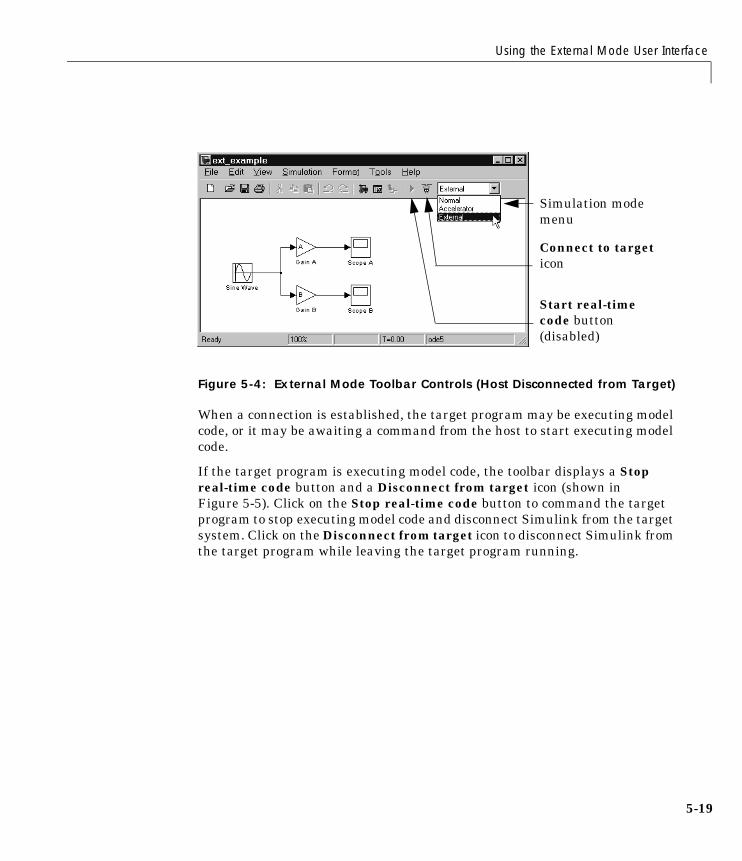
Using the External Mode User Interface
5-19
Figure 5-4: External Mode Toolbar Controls (Host Disconnected from Target)
When a connection is established, the target program may be executing modelcode, or it may be awaiting a command from the host to start executing modelcode.
If the target program is executing model code, the toolbar displays a Stopreal-time code button and a Disconnect from target icon (shown inFigure 5-5). Click on the Stop real-time code button to command the targetprogram to stop executing model code and disconnect Simulink from the targetsystem. Click on the Disconnect from target icon to disconnect Simulink fromthe target program while leaving the target program running.
Simulation modemenu
Connect to targeticon
Start real-timecode button(disabled)
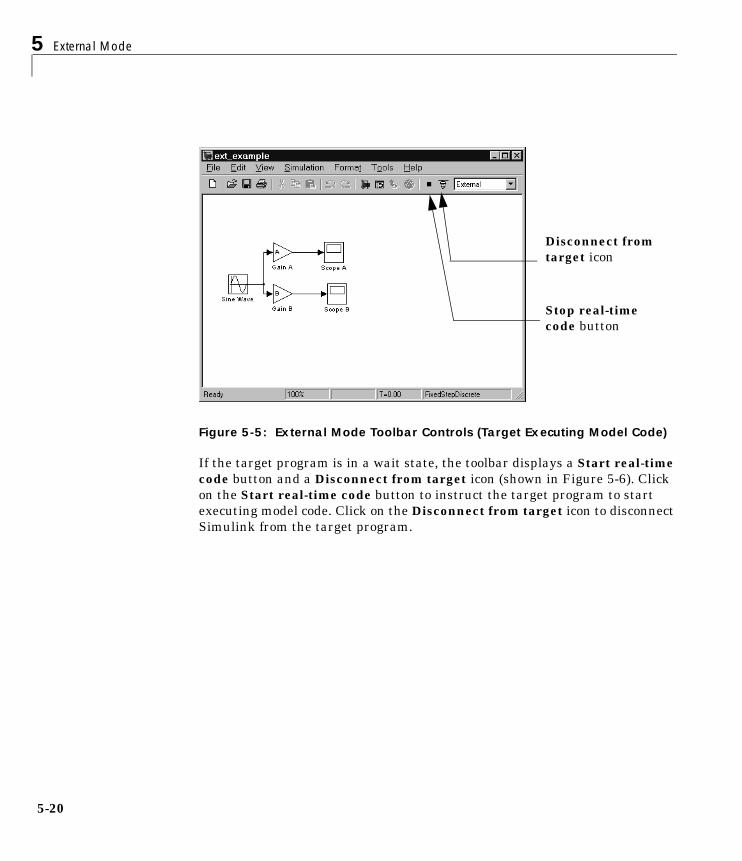
5 External Mode
5-20
Figure 5-5: External Mode Toolbar Controls (Target Executing Model Code)
If the target program is in a wait state, the toolbar displays a Start real-timecode button and a Disconnect from target icon (shown in Figure 5-6). Clickon the Start real-time code button to instruct the target program to startexecuting model code. Click on the Disconnect from target icon to disconnectSimulink from the target program.
Disconnect fromtarget icon
Stop real-timecode button
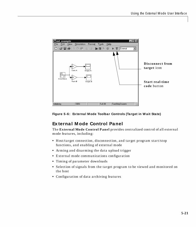
Using the External Mode User Interface
5-21
Figure 5-6: External Mode Toolbar Controls (Target in Wait State)
External Mode Control PanelThe External Mode Control Panel provides centralized control of all externalmode features, including:
• Host/target connection, disconnection, and target program start/stopfunctions, and enabling of external mode
• Arming and disarming the data upload trigger
• External mode communications configuration
• Timing of parameter downloads
• Selection of signals from the target program to be viewed and monitored onthe host
• Configuration of data archiving features
Disconnect fromtarget icon
Start real-timecode button
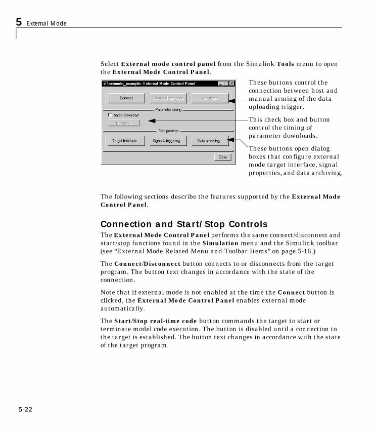
5 External Mode
5-22
Select External mode control panel from the Simulink Tools menu to openthe External Mode Control Panel.
The following sections describe the features supported by the External ModeControl Panel.
Connection and Start/Stop ControlsThe External Mode Control Panel performs the same connect/disconnect andstart/stop functions found in the Simulation menu and the Simulink toolbar(see “External Mode Related Menu and Toolbar Items” on page 5-16.)
The Connect/Disconnect button connects to or disconnects from the targetprogram. The button text changes in accordance with the state of theconnection.
Note that if external mode is not enabled at the time the Connect button isclicked, the External Mode Control Panel enables external modeautomatically.
The Start/Stop real-time code button commands the target to start orterminate model code execution. The button is disabled until a connection tothe target is established. The button text changes in accordance with the stateof the target program.
These buttons control theconnection between host andmanual arming of the datauploading trigger.
This check box and buttoncontrol the timing ofparameter downloads.
These buttons open dialogboxes that configure externalmode target interface, signalproperties, and data archiving.

Using the External Mode User Interface
5-23
Target Interface Dialog BoxPressing the Target Interface button activates the External TargetInterface dialog box.
The External Target Interface dialog box lets you specify the name of aMEX-file that implements host/target communications. This is known as theexternal interface MEX-file. The fields of the External Target Interface dialogbox are:
• MEX-file for external interface: Name of the external interface MEX-file.The default is ext_comm, the TCP/IP-based external interface file providedfor use with the GRT and Tornado targets
The external interface MEX-file for the Real-Time Windows Target iswin_tgt.
Custom or third-party targets may use a different external interfaceMEX-file.
• MEX-file arguments: Arguments for the external interface MEX-file. Forexample, ext_comm allows three optional arguments: the network name ofyour target, the verbosity level, and a TCP/IP server port number.
See “The External Interface MEX-File” on page 5-40 for details on ext_command its arguments.
Specify name of externalinterface MEX-file here. Defaultis ext_comm.
Enter optional arguments to the external interface MEX-file here.
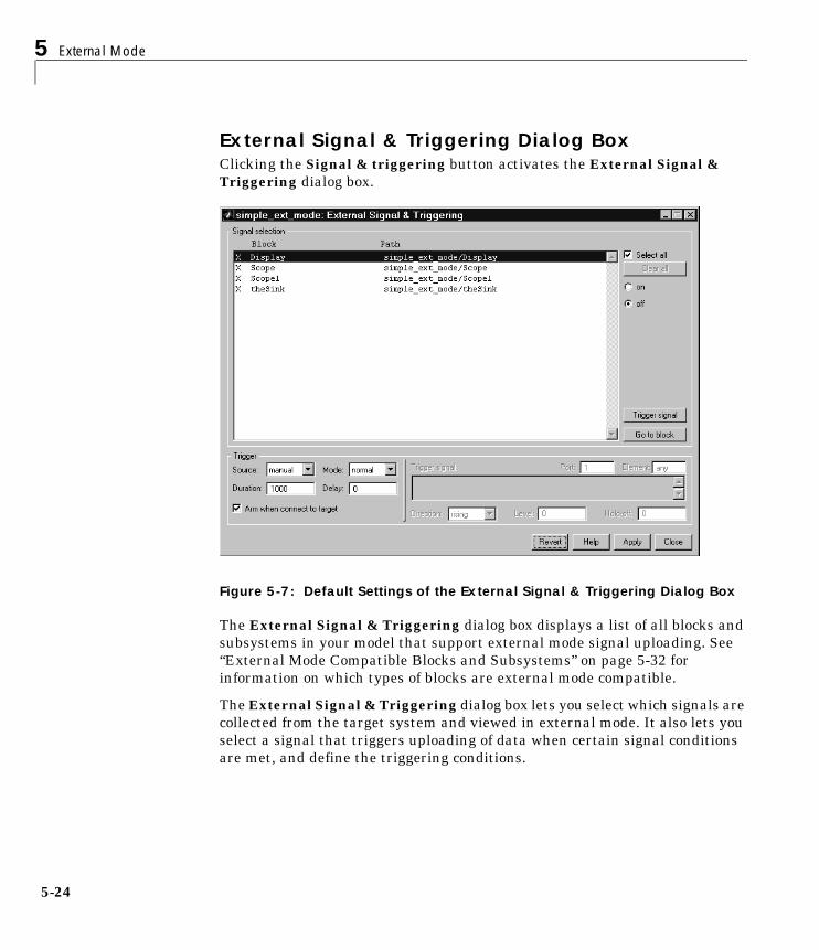
5 External Mode
5-24
External Signal & Triggering Dialog BoxClicking the Signal & triggering button activates the External Signal &Triggering dialog box.
Figure 5-7: Default Settings of the External Signal & Triggering Dialog Box
The External Signal & Triggering dialog box displays a list of all blocks andsubsystems in your model that support external mode signal uploading. See“External Mode Compatible Blocks and Subsystems” on page 5-32 forinformation on which types of blocks are external mode compatible.
The External Signal & Triggering dialog box lets you select which signals arecollected from the target system and viewed in external mode. It also lets youselect a signal that triggers uploading of data when certain signal conditionsare met, and define the triggering conditions.
Using the External Mode User Interface
5-25
Default OperationFigure 5-7 shows the default settings of the External Signal and Triggeringdialog box. The default operation of the External Signal and Triggeringdialog box is designed to simplify monitoring the target program. If you use thedefault settings, you do not need to preconfigure signals and triggers. Simplystart the target program and connect the Simulink model to it. All externalmode compatible blocks will be selected and the trigger will be armed. Signaluploading will begin immediately upon connection to the target program.
The default configuration is:
• Arm when connect to target: on
• Trigger Mode: normal
• Trigger Source: manual
• Select all: on
Signal SelectionAll external mode compatible blocks in your model appear in the Signalselection list of the External Signal & Triggering dialog box. You use this listto select signals to be viewed. An X appears to the left of each selected block’sname.
The Select all check box selects all signals. By default, Select all is on.
If Select all is off, you can select or deselect individual signals using the on andoff radio buttons. To select a signal, click on the desired list entry and click theon radio button. To deselect a signal, click on the desired list entry and clickthe off radio button. Alternatively, you can double-click a signal in the list totoggle between selection and deselection.
The Clear all button deselects all signals.
Trigger OptionsThe Trigger panel located at the bottom left of the External Signal &Triggering dialog box contains options that control when and how signal datais collected (uploaded) from the target system. These options are:
5 External Mode
5-26
• Source: manual or signal. Selecting manual directs external mode to startlogging data when the Arm trigger button on the External Mode ControlPanel is clicked.
Selecting signal tells external mode to start logging data when a selectedtrigger signal satisfies trigger conditions specified in the Trigger signalpanel. When the trigger conditions are satisfied (that is, the signal crossesthe trigger level in the specified direction) a trigger event occurs. If thetrigger is armed, external mode monitors for the occurrence of a triggerevent. When a trigger event occurs, data logging begins.
• Arm when connect to target: If this option is selected, external mode armsthe trigger automatically when Simulink has connected to the target. If thetrigger source is manual, uploading begins immediately. If the trigger modeis signal, monitoring of the trigger signal begins immediately, anduploading begins upon the occurrence of a trigger event.
If Arm when connect to target is not selected, you must manually arm thetrigger by clicking the Arm trigger button in the External Mode ControlPanel.
• Duration: The number of base rate steps for which external mode logs dataafter a trigger event. For example, if the fastest rate in the model is 1 secondand a signal sampled at 1 Hz is being logged for a duration of 10 seconds,then external mode will collect 10 samples. If a signal sampled at 2 Hz islogged, only 5 samples will be collected.
• Mode: normal or one-shot. In normal mode, external mode automaticallyrearms the trigger after each trigger event. In one-shotmode, external modecollects only one buffer of data each time you arm the trigger. See “DataArchiving” on page 5-28 for further details on the effect of the Mode setting.
• Delay: The delay represents the amount of time that elapses between atrigger occurrence and the start of data collection. The delay is expressed inbase rate steps, and can be positive or negative. A negative delay correspondsto pretriggering. When the delay is negative, data from the time precedingthe trigger is collected and uploaded.
Trigger Signal SelectionYou can designate one signal as a trigger signal. To select a trigger signal,select signal from the Trigger Source menu. This activates the Triggersignal panel (see Figure 5-8). Then, click on the desired entry in the Signalselection list, and click the Trigger signal button.
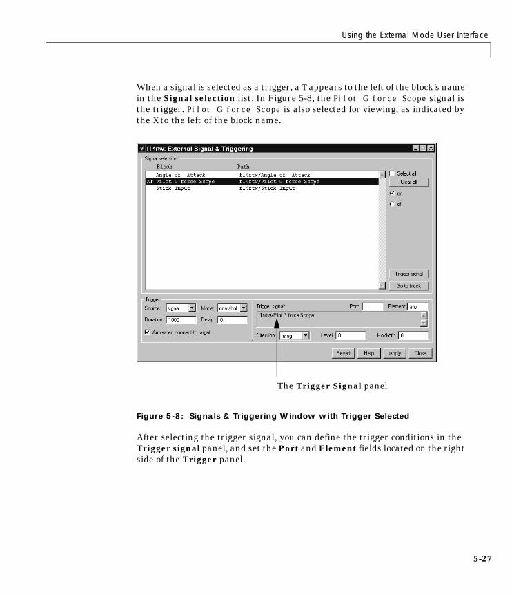
Using the External Mode User Interface
5-27
When a signal is selected as a trigger, a T appears to the left of the block’s namein the Signal selection list. In Figure 5-8, the Pilot G force Scope signal isthe trigger. Pilot G force Scope is also selected for viewing, as indicated bythe X to the left of the block name.
Figure 5-8: Signals & Triggering Window with Trigger Selected
After selecting the trigger signal, you can define the trigger conditions in theTrigger signal panel, and set the Port and Element fields located on the rightside of the Trigger panel.
The Trigger Signal panel
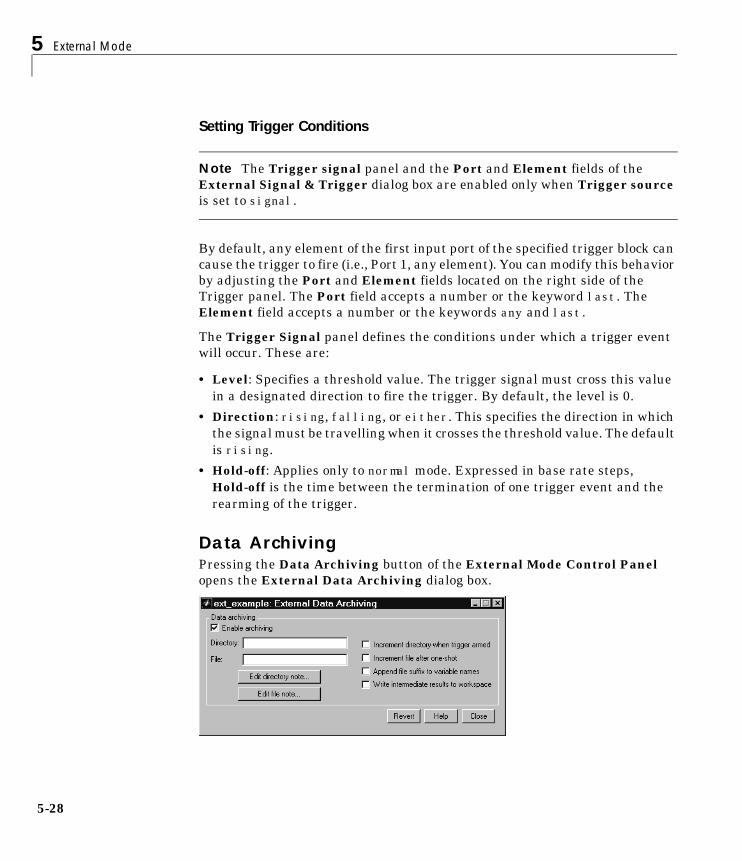
5 External Mode
5-28
Setting Trigger Conditions
Note The Trigger signal panel and the Port and Element fields of theExternal Signal & Trigger dialog box are enabled only when Trigger sourceis set to signal.
By default, any element of the first input port of the specified trigger block cancause the trigger to fire (i.e., Port 1, any element). You can modify this behaviorby adjusting the Port and Element fields located on the right side of theTrigger panel. The Port field accepts a number or the keyword last. TheElement field accepts a number or the keywords any and last.
The Trigger Signal panel defines the conditions under which a trigger eventwill occur. These are:
• Level: Specifies a threshold value. The trigger signal must cross this valuein a designated direction to fire the trigger. By default, the level is 0.
• Direction: rising, falling, or either. This specifies the direction in whichthe signal must be travelling when it crosses the threshold value. The defaultis rising.
• Hold-off: Applies only to normal mode. Expressed in base rate steps,Hold-off is the time between the termination of one trigger event and therearming of the trigger.
Data ArchivingPressing the Data Archiving button of the External Mode Control Panelopens the External Data Archiving dialog box.
Using the External Mode User Interface
5-29
This panel supports the following features:
Directory Notes. Use this option to add annotations that pertain to a collection ofrelated data files in a directory.
Pressing the Edit directory note button opens the MATLAB editor. Placecomments that you want saved to a file in the specified directory in thiswindow. By default, the comments are saved to the directory last written to bydata archiving.
File Notes. Pressing Edit file note opens a file finder window that is, by default,set to the last file to which you have written. Selecting any MAT-file opens anedit window. Add or edit comments in this window that you want saved withyour individual MAT-file.
Data Archiving. Clicking the Enable Archiving check box activates theautomated data archiving features of external mode. To understand how thearchiving features work, it is necessary to consider the handling of data whenarchiving is not enabled. There are two cases, one-shot and normal mode.
In one-shot mode, after a trigger event occurs, each selected block writes itsdata to the workspace just as it would at the end of a simulation. If anotherone-shot is triggered, the existing workspace data will be overwritten.
In normal mode, external mode automatically rearms the trigger after eachtrigger event. Consequently, you can think of normal mode as a series ofone-shots. Each one-shot in this series, except for the last, is referred to as anintermediate result. Since the trigger can fire at any time, writing intermediateresults to the workspace generally results in unpredictable overwriting of theworkspace variables. For this reason, the default behavior is to write only theresults from the final one-shot to the workspace. The intermediate results arediscarded. If you know that sufficient time exists between triggers forinspection of the intermediate results, then you can override the defaultbehavior by checking the Write intermediate results to workspace check box.Note that this option does not protect the workspace data from beingoverwritten by subsequent triggers.
The options in the External Data Archiving dialog box support automaticwriting of logging results, including intermediate results, to disk. Dataarchiving provides the following settings:
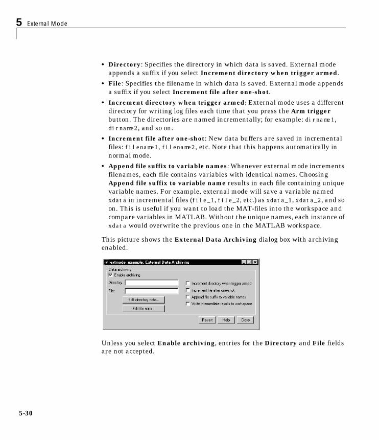
5 External Mode
5-30
• Directory: Specifies the directory in which data is saved. External modeappends a suffix if you select Increment directory when trigger armed.
• File: Specifies the filename in which data is saved. External mode appendsa suffix if you select Increment file after one-shot.
• Increment directory when trigger armed: External mode uses a differentdirectory for writing log files each time that you press the Arm triggerbutton. The directories are named incrementally; for example: dirname1,dirname2, and so on.
• Increment file after one-shot: New data buffers are saved in incrementalfiles: filename1, filename2, etc. Note that this happens automatically innormal mode.
• Append file suffix to variable names: Whenever external mode incrementsfilenames, each file contains variables with identical names. ChoosingAppend file suffix to variable name results in each file containing uniquevariable names. For example, external mode will save a variable namedxdata in incremental files (file_1, file_2, etc.) as xdata_1, xdata_2, and soon. This is useful if you want to load the MAT-files into the workspace andcompare variables in MATLAB. Without the unique names, each instance ofxdata would overwrite the previous one in the MATLAB workspace.
This picture shows the External Data Archiving dialog box with archivingenabled.
Unless you select Enable archiving, entries for the Directory and File fieldsare not accepted.
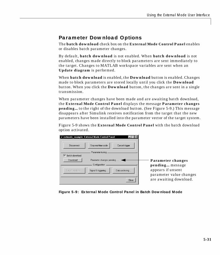
Using the External Mode User Interface
5-31
Parameter Download OptionsThe batch download check box on the External Mode Control Panel enablesor disables batch parameter changes.
By default, batch download is not enabled. When batch download is notenabled, changes made directly to block parameters are sent immediately tothe target. Changes to MATLAB workspace variables are sent when anUpdate diagram is performed.
When batch download is enabled, the Download button is enabled. Changesmade to block parameters are stored locally until you click the Downloadbutton. When you click the Download button, the changes are sent in a singletransmission.
When parameter changes have been made and are awaiting batch download,the External Mode Control Panel displays the message Parameter changespending... to the right of the download button. (See Figure 5-9.) This messagedisappears after Simulink receives notification from the target that the newparameters have been installed into the parameter vector of the target system.
Figure 5-9 shows the External Mode Control Panel with the batch downloadoption activated.
Figure 5-9: External Mode Control Panel in Batch Download Mode
Parameter changespending... messageappears if unsentparameter value changesare awaiting download.
5 External Mode
5-32
External Mode Compatible Blocks and Subsystems
Compatible BlocksIn external mode, you can use the following types of blocks to receive and viewsignals uploaded from the target program:
• Scope blocks
• Blocks in the Dials & Gauges Blockset
• Display blocks
• To Workspace blocks
• User-written S-Function blocks
An external mode method has been added to the S-function API. This methodallows user-written blocks to support external mode. See matlabroot/simulink/simstruc.h.
• XY Graph blocks
In addition to these types of blocks, you can designate certain subsystems asSignal Viewing Subsystems and use them to receive and view signals uploadedfrom the target program. See “Signal Viewing Subsystems” on page 5-32 forfurther information.
External mode compatible blocks and subsystems are selected, and the triggeris armed, via the External Signal and Triggering dialog box. For example,Figure 5-7 shows two Scope blocks, a Display block, and a Signal ViewingSubsystem (theSink). All of these are selected and the trigger is set to be armedwhen connected to the target program.
Signal Viewing SubsystemsA Signal Viewing Subsystem is an atomic subsystem that encapsulatesprocessing and viewing of signals received from the target system. A SignalViewing Subsystem runs only on the host, generating no code in the targetsystem. Signal Viewing Subsystems run in all simulation modes — normal,accelerated, and external.
Signal Viewing Subsystems are useful in situations where you want to processor condition signals before viewing or logging them, but you do not want toperform these tasks on the target system. By using a Signal Viewing
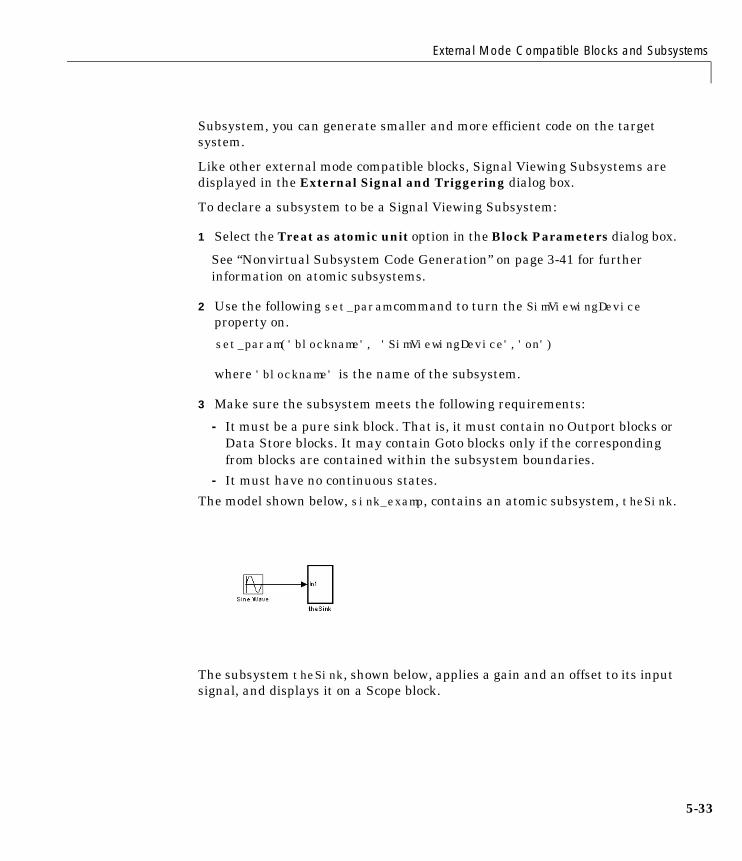
External Mode Compatible Blocks and Subsystems
5-33
Subsystem, you can generate smaller and more efficient code on the targetsystem.
Like other external mode compatible blocks, Signal Viewing Subsystems aredisplayed in the External Signal and Triggering dialog box.
To declare a subsystem to be a Signal Viewing Subsystem:
1 Select the Treat as atomic unit option in the Block Parameters dialog box.
See “Nonvirtual Subsystem Code Generation” on page 3-41 for furtherinformation on atomic subsystems.
2 Use the following set_param command to turn the SimViewingDeviceproperty on.
set_param('blockname', 'SimViewingDevice','on')
where 'blockname' is the name of the subsystem.
3 Make sure the subsystem meets the following requirements:
- It must be a pure sink block. That is, it must contain no Outport blocks orData Store blocks. It may contain Goto blocks only if the correspondingfrom blocks are contained within the subsystem boundaries.
- It must have no continuous states.
The model shown below, sink_examp, contains an atomic subsystem, theSink.
The subsystem theSink, shown below, applies a gain and an offset to its inputsignal, and displays it on a Scope block.

5 External Mode
5-34
If theSink is declared as a Signal Viewing Subsystem, the generated targetprogram includes only the code for the Sine Wave block. If theSink is selectedand armed in the External Signal and Triggering dialog box (as shown inFigure 5-10), the target program uploads the sine wave signal to theSinkduring simulation.You can then modify the parameters of the blocks withintheSink and observe their effect upon the uploaded signal.
Figure 5-10: Signal Viewing Subsystem Selected in ExternalSignals & Triggering Dialog Box

External Mode Compatible Blocks and Subsystems
5-35
Note that if theSink were not declared as a Signal Viewing Subsystem, itsGain, Constant, and Sum blocks would run as subsystem code on the targetsystem. The Sine Wave signal would be uploaded to Simulink after beingprocessed by these blocks, and viewed on sink_examp/theSink/Scope2.Processing demands on the target system would be increased by the additionalsignal processing, and by the downloading of block parameter changes from thehost.
5 External Mode
5-36
Overview of External Mode CommunicationsIn external mode, Simulink does not simulate the system represented by theblock diagram. When external mode is enabled, Simulink downloads currentvalues of all parameters to the target system. After the initial download,Simulink remains in a waiting mode until you change parameters in the blockdiagram or until Simulink receives data from the target.
The Download MechanismWhen you change a parameter in the block diagram, Simulink calls theexternal interface MEX-file, passing new parameter values (along with otherinformation) as arguments.
The external interface MEX-file contains code that implements one side of theinterprocess communication (IPC) channel. This channel connects theSimulink process (where the MEX-file executes) to the process that is executingthe external program. The MEX-file transfers the new parameter values viathis channel to the external program.
The other side of the communication channel is implemented within theexternal program. This side writes the new parameter values into target’sparameter structure (rtP).
The Simulink side initiates the parameter download operation by sending amessage containing parameter information to the external program. In theterminology of client/server computing, the Simulink side is the client and theexternal program is the server. The two processes can be remote, or they canbe local. Where the client and server are remote, a protocol such as TCP/IP isused to transfer data. Where the client and server are local, shared memory canbe used to transfer data.
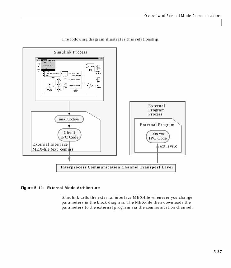
Overview of External Mode Communications
5-37
The following diagram illustrates this relationship.
Figure 5-11: External Mode Architecture
Simulink calls the external interface MEX-file whenever you changeparameters in the block diagram. The MEX-file then downloads theparameters to the external program via the communication channel.
External Program
IPC CodeServer
ExternalProgramProcess
Simulink Process
IPC CodeClient
mexFunction
External InterfaceMEX-file (ext_comm)
ext_svr.c
Interprocess Communication Channel Transport Layer

5 External Mode
5-38
The TCP/IP Implementation
OverviewThe Real-Time Workshop provides code to implement both the client andserver side based on TCP/IP. You can use the socket-based external modeimplementation provided by the Real-Time Workshop with the generated code,provided that your target system supports TCP/IP.
A low-level transport layer handles physical transmission of messages. BothSimulink and the model code are independent of this layer. Both the transportlayer and code directly interfacing to the transport layer are isolated inseparate modules that format, transmit, and receive messages and datapackets.
This design makes it possible for different targets to use different transportlayers. For example, the grt, grt_malloc, and Tornado targets support host/target communication via TCP/IP, whereas the xPC target supports bothRS232 (serial) and TCP/IP communication.
Using the TCP/IP ImplementationThis section discusses how to use the TCP/IP-based client/serverimplementation of external mode with real-time programs on a UNIX or PCsystem. Chapter 12, “Targeting Tornado for Real-Time Applications”illustrates the use of external mode in the Tornado environment.
In order to use Simulink external mode, you must:
• Specify the name of the external interface MEX-file in the External TargetInterface dialog box. By default, this is ext_comm.
• Configure the template makefile so that it links the proper source files forthe TCP/IP server code and defines the necessary compiler flags whenbuilding the generated code.
• Build the external program.
• Run the external program.
• Set Simulink to external mode and connect to the target.

The TCP/IP Implementation
5-39
This figure shows the structure of the TCP/IP-based implementation.
Figure 5-12: TCP/IP-Based Client/Server Implementation for External Mode
The following sections discuss the details of how to use the external mode ofSimulink.
ext_comm
Process blockparameter
TCP/IP on Ethernet
Target Code
ext_svr.c
Simulink in External Mode
UNIX or PC Host Target
Update block
header data in target format
External Mode Message Format

5 External Mode
5-40
The External Interface MEX-FileYou must specify the name of the external interface MEX-file in the ExternalTarget Interface dialog box.
The default external interface MEX-file is ext_comm. ext_comm implementsTCP/IP-based communications. ext_comm has three optional arguments,discussed in the next section.
MEX-File Optional ArgumentsIn the External Target Interface dialog box, you can specify optionalarguments that are passed to the MEX-file. These are:
• Target network name: the network name of the computer running theexternal program. By default, this is the computer on which Simulink isrunning. The name can be:
- a string delimited by single quotes, such as 'myPuter'
- an IP address delimited by single quotes, such as '148.27.151.12'
• Verbosity level: controls the level of detail of the information displayedduring the data transfer. The value is either 0 or 1 and has the followingmeaning:
0 — no information
1 — detailed information
• TCP/IP server port number: The default value is 17725. You can change theport number to a value between 256 and 65535 to avoid a port conflict ifnecessary.
Enter the name of the externalinterface MEX-file in the box(you do not need to enter the.mex extension). This file mustbe in the current directory or in adirectory that is on yourMATLAB path.

The TCP/IP Implementation
5-41
You must specify these options in order. For example, if you want to specify theverbosity level (the second argument), then you must also specify the targethost name (the first argument).
Note that you can specify command line options to the external program. See“Running the External Program” on page 5-41 for more information.
External Mode Compatible TargetsThe GRT and Tornado targets support external mode. To enable external modecode generation, check External mode in the target-specific code generationoptions section of the Real-Time Workshop page. The following illustrationshows the GRT code generation options with external mode enabled.
Running the External ProgramThe external program must be running before you can use Simulink in externalmode. To run the external program, you type a command of the form
model -opt1 ... -optN
where model is the name of the external program and -opt1 ... -optN areoptions. (See “Command Line Options for the External Program” on page 5–42). In the examples in this section, we assume the name of the externalprogram to be ext_example.
5 External Mode
5-42
Running the External Program Under WindowsIn the Windows environment, you can run the external programs in either ofthe following ways:
• Open an MS-DOS command prompt. At the command prompt, type the nameof the target executable, followed by any options, as in the following example.ext_example -tf inf -w
• Alternatively, you can launch the target executable from the MATLABcommand prompt. In this case the command must be preceded by anexclamation point (!) and followed by an ampersand (&) , as in the followingexample.
!ext_example -tf inf -w &
Running the External Program Under UNIXIn the UNIX environment, you can run the external programs in either of thefollowing ways:
• Open an an Xterm window. At the command prompt, type the name of thetarget executable, followed by any options, as in the following example.ext_example -tf inf -w
• Alternatively, you can launch the target executable from the MATLABcommand prompt. In the UNIX environment, if you start the externalprogram from MATLAB, you must run it in the background so that you canstill access Simulink. The command must be preceded by an exclamationpoint (!) and followed by an ampersand (&) , as in the following example.!ext_example -tf inf -w &
runs the executable from MATLAB by spawning another process to run it.
Command Line Options for the External ProgramExternal mode target executables generated by the Real-Time Workshopsupport the following command line options:
• -tf n option
The -tf option overrides the stop time set for the model in Simulink. Theargument n specifies the number of seconds the program will run. The value
The TCP/IP Implementation
5-43
inf value directs the model to run indefinitely. In this case, the model codewill run until the target program receives a stop message from Simulink.
The following example sets the stop time to 10 seconds.ext_example -tf 10
Note The -tf option is supported by the GRT and Tornado targets. If you areimplementing a custom target and want to support the -tf option, you mustimplement the option yourself. See “Creating an External ModeCommunication Channel” on page 17–73 for further information.
• -w option
The -w option instructs the target program to enter a wait state until itreceives a message from the host. At this point, the target is running, but notexecuting the model code. The start message is sent when you select Startreal-time code from the Simulation menu or click the Start real-time codebutton in the External Mode Control Panel.
Use the -w option if you want to view data from time step 0 of the targetprogram execution, or if you want to modify parameters before the targetprogram begins execution of model code.
• -port n option
the -port option specifies the TCP/IP port number, n, for the target program.The port number of the target program must match that of the host. Thedefault port number is 17725. The port number must be a value between 256and 65535.
Note The -w and -port options are supported by the TCP/IP transport layermodules shipped with the Real-Time Workshop. By default, these modules arelinked into external mode target executables. If you are implementing acustom external mode transport layer and want to support these options, youmust implement them in your code. See “Creating an External ModeCommunication Channel” on page 17–73 for further information. Seematlabroot/rtw/c/src/ext_transport.c for example code.
5 External Mode
5-44
Error ConditionsIf the Simulink block diagram does not match the external program, Simulinkdisplays an error box informing you that the checksums do not match (i.e., themodel has changed since you generated code). This means you must rebuild theprogram from the new block diagram (or reload the correct one) in order to useexternal mode.
If the external program is not running, Simulink displays an error informingyou that it cannot connect to the external program.
Implementing an External Mode Protocol LayerIf you want to implement your own transport layer for external modecommunication, you must modify certain code modules provided by theReal-Time Workshop, and rebuild ext_comm, the external interface MEX-file.This advanced topic is described in detail in “Creating an External ModeCommunication Channel” on page 17–73.

Limitations of External Mode
5-45
Limitations of External ModeIn general, you cannot change a parameter if doing so results in a change in thestructure of the model. For example, you cannot change:
• The number of states, inputs, or outputs of any block
• The sample time or the number of sample times
• The integration algorithm for continuous systems
• The name of the model or of any block
• The parameters to the Fcn block
If you cause any of these changes to the block diagram, then you must rebuildthe program with newly generated code.
However, parameters in transfer function and state space representationblocks can be changed in specific ways:
• The parameters (numerator and denominator polynomials) for the TransferFcn (continuous and discrete) and Discrete Filter blocks can be changed (aslong as the number of states does not change).
• Zero entries in the State Space and Zero Pole (both continuous and discrete)blocks in the user-specified or computed parameters (i.e., the A, B, C, and Dmatrices obtained by a zero-pole to state-space transformation) cannot bechanged once external simulation is started.
• In the State Space blocks, if you specify the matrices in the controllablecanonical realization, then all changes to the A, B, C, D matrices thatpreserve this realization and the dimensions of the matrices are allowed.

5 External Mode
5-46
6
Program Architecture
Introduction . . . . . . . . . . . . . . . . . . . . 6-2
Model Execution . . . . . . . . . . . . . . . . . . 6-5Program Timing . . . . . . . . . . . . . . . . . . . 6-13Program Execution . . . . . . . . . . . . . . . . . . 6-14External Mode Communication . . . . . . . . . . . . . 6-14Data Logging In Single-
and Multitasking Model Execution . . . . . . . . . 6-14Rapid Prototyping and Embedded
Model Execution Differences . . . . . . . . . . . . 6-15Rapid Prototyping Model Functions . . . . . . . . . . . 6-16Embedded Model Functions . . . . . . . . . . . . . . 6-22
Rapid Prototyping Program Framework . . . . . . . 6-24Rapid Prototyping Program Architecture . . . . . . . . . 6-25Rapid Prototyping System Dependent Components . . . . . 6-26Rapid Prototyping System Independent Components . . . . 6-27Rapid Prototyping Application Components . . . . . . . . 6-30
Embedded Program Framework . . . . . . . . . . . 6-35
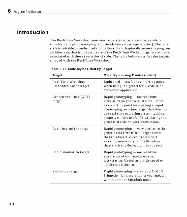
6 Program Architecture
6-2
IntroductionThe Real-Time Workshop generates two styles of code. One code style issuitable for rapid prototyping (and simulation via code generation). The otherstyle is suitable for embedded applications. This chapter discusses the programarchitecture, that is, the structure of the Real-Time Workshop generated code,associated with these two styles of code. The table below classifies the targetsshipped with the Real-Time Workshop.
Table 6-1: Code Styles Listed By Target
Target Code Style (using C unless noted)
Real-Time WorkshopEmbedded Coder target
Embedded — useful as a starting pointwhen using the generated C code in anembedded application.
Generic real-time (GRT)target
Rapid prototyping — nonreal-timesimulation on your workstation. Usefulas a starting point for creating a rapidprototyping real-time target that does notuse real-time operating system taskingprimitives. Also useful for validating thegenerated code on your workstation.
Real-time malloc target Rapid prototyping — very similar to thegeneric real-time (GRT) target exceptthat this target allocates all modelworking memory dynamically ratherthan statically declaring it in advance.
Rapid simulation target Rapid prototyping — nonreal-timesimulation of your model on yourworkstation. Useful as a high-speed orbatch simulation tool.
S-function target Rapid prototyping — creates a C-MEXS-function for simulation of your modelwithin another Simulink model.

6-3
Third-party vendors supply additional targets for the Real-Time Workshop.Generally, these can be classified as rapid prototyping targets. For moreinformation about third-party products, see the MATLAB Connections Webpage: http://www.mathworks.com/products/connections.
You can identify the rapid prototyping style of generated code by its use of theSimStruct data structure (i.e., #include "simstruc.h"). In contrast, theembedded code style does not have a SimStruct.
Tornado (VxWorks) real-timetarget
Rapid prototyping — runs model in realtime using the VxWorks real-timeoperating system tasking primitives. Alsouseful as a starting point for targeting areal-time operating system.
Real-Time Windows target Rapid prototyping — runs model inreal-time at interrupt level while your PCis running Microsoft Windows in thebackground.
Ada simulation target Embedded — nonreal-time simulation onyour workstation using Ada. Useful forvalidating the generated code on yourworkstation.
Ada multitasking real-timetarget
Embedded — uses Ada tasking primitivesto run your model in real time. Useful asa starting point when using thegenerated Ada code in an embeddedapplication.
xPC target Rapid prototyping — runs model in realtime on target PC running xPC kernel.
DOS real-time target Rapid prototyping — runs model in realtime at interrupt level under DOS.
Table 6-1: Code Styles Listed By Target (Continued)
Target Code Style (using C unless noted)

6 Program Architecture
6-4
This chapter is divided into three sections. The first section discusses modelexecution; the second section discusses the rapid prototyping style of code; andthe third section discusses the embedded style of code.
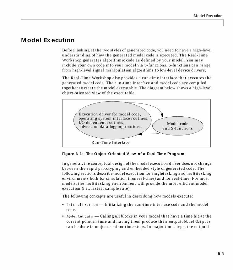
Model Execution
6-5
Model ExecutionBefore looking at the two styles of generated code, you need to have a high-levelunderstanding of how the generated model code is executed. The Real-TimeWorkshop generates algorithmic code as defined by your model. You mayinclude your own code into your model via S-functions. S-functions can rangefrom high-level signal manipulation algorithms to low-level device drivers.
The Real-Time Workshop also provides a run-time interface that executes thegenerated model code. The run-time interface and model code are compiledtogether to create the model executable. The diagram below shows a high-levelobject-oriented view of the executable.
Figure 6-1: The Object-Oriented View of a Real-Time Program
In general, the conceptual design of the model execution driver does not changebetween the rapid prototyping and embedded style of generated code. Thefollowing sections describe model execution for singletasking and multitaskingenvironments both for simulation (nonreal-time) and for real-time. For mostmodels, the multitasking environment will provide the most efficient modelexecution (i.e., fastest sample rate).
The following concepts are useful in describing how models execute:
• Initialization — Initializing the run-time interface code and the modelcode.
• ModelOutputs — Calling all blocks in your model that have a time hit at thecurrent point in time and having them produce their output. ModelOutputscan be done in major or minor time steps. In major time steps, the output is
Model codeand S-functions
Run-Time Interface
Execution driver for model code,operating system interface routines,I/O dependent routines,solver and data logging routines.

6 Program Architecture
6-6
a given simulation time step. In minor time steps, the run-time interfaceintegrates the derivatives to update the continuous states.
• ModelUpdate— Calling all blocks in your model that have a sample hit at thecurrent point in time and having them update their discrete states or similartype objects.
• ModelDerivatives — Calling all blocks in your model that have continuousstates and having them update their derivatives. ModelDerivatives is onlycalled in minor time steps.
The pseudocode below shows the execution of a model for a singletaskingsimulation (nonreal-time).
main(){InitializationWhile (time < final time)ModelOutputs -- Major time step.LogTXY -- Log time, states and root outports.ModelUpdate -- Major time step.Integrate: -- Integration in minor time step for models
-- with continuous states.ModelDerivativesDo 0 or more:
ModelOutputsModelDerivatives
EndDo (Number of iterations depends upon the solver.)Integrate derivatives to update continuous states.
EndIntegrateEndWhileShutdown
}
The initialization phase begins first. This consists of initializing model statesand setting up the execution engine. The model then executes, one step at atime. First ModelOutputs executes at time t, then the workspace I/O data islogged, and then ModelUpdate updates the discrete states. Next, if your modelhas any continuous states, ModelDerivatives integrates the continuous states’derivatives to generate the states for time , where h is the step
size. Time then moves forward to and the process repeats.
tnew t h+=
tnew

Model Execution
6-7
During the ModelOutputs and ModelUpdate phases of model execution, onlyblocks that have hit the current point in time execute. They determine if theyhave hit by using a macro (ssIsSampleHit, or ssIsSpecialSampleHit) thatchecks for a sample hit.
The pseudocode below shows the execution of a model for a multitaskingsimulation (nonreal-time).
main(){
InitializationWhile (time < final time)ModelOutputs(tid=0) -- Major time step.LogTXY -- Log time, states, and root outports.ModelUpdate(tid=1) -- Major time step.For i=1:NumTidsModelOutputs(tid=i) -- Major time step.ModelUpdate(tid=i) -- Major time step.
EndForIntegrate -- Integration in minor time step for models
-- with continuous states.ModelDerivativesDo 0 or more:ModelOutputs(tid=0)ModelDerivatives
EndDo (Number of iterations depends upon the solver.)Integrate derivatives to update continuous states.
EndIntegrateEndWhileShutdown}
The multitasking operation is more complex when compared with thesingletasking execution because the output and update functions aresubdivided by the task identifier (tid) that is passed into these functions. Thisallows for multiple invocations of these functions with different task identifiersusing overlapped interrupts, or for multiple tasks when using a real-timeoperating system. In simulation, multiple tasks are emulated by executing thecode in the order that would occur if there were no preemption in a real-timesystem.
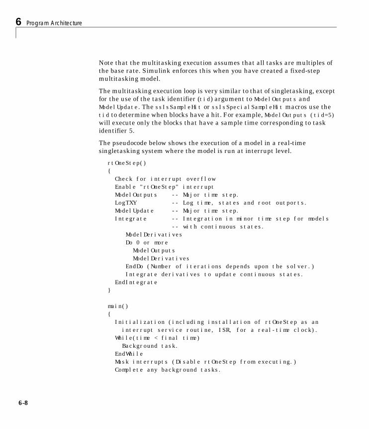
6 Program Architecture
6-8
Note that the multitasking execution assumes that all tasks are multiples ofthe base rate. Simulink enforces this when you have created a fixed-stepmultitasking model.
The multitasking execution loop is very similar to that of singletasking, exceptfor the use of the task identifier (tid) argument to ModelOutputs andModelUpdate. The ssIsSampleHit or ssIsSpecialSampleHit macros use thetid to determine when blocks have a hit. For example, ModelOutputs (tid=5)will execute only the blocks that have a sample time corresponding to taskidentifier 5.
The pseudocode below shows the execution of a model in a real-timesingletasking system where the model is run at interrupt level.
rtOneStep(){Check for interrupt overflowEnable "rtOneStep" interruptModelOutputs -- Major time step.LogTXY -- Log time, states and root outports.ModelUpdate -- Major time step.Integrate -- Integration in minor time step for models
-- with continuous states.ModelDerivativesDo 0 or more
ModelOutputsModelDerivatives
EndDo (Number of iterations depends upon the solver.)Integrate derivatives to update continuous states.
EndIntegrate}
main(){Initialization (including installation of rtOneStep as an interrupt service routine, ISR, for a real-time clock).
While(time < final time)Background task.
EndWhileMask interrupts (Disable rtOneStep from executing.)Complete any background tasks.
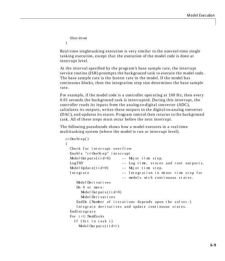
Model Execution
6-9
Shutdown}
Real-time singletasking execution is very similar to the nonreal-time singletasking execution, except that the execution of the model code is done atinterrupt level.
At the interval specified by the program’s base sample rate, the interruptservice routine (ISR) preempts the background task to execute the model code.The base sample rate is the fastest rate in the model. If the model hascontinuous blocks, then the integration step size determines the base samplerate.
For example, if the model code is a controller operating at 100 Hz, then every0.01 seconds the background task is interrupted. During this interrupt, thecontroller reads its inputs from the analog-to-digital converter (ADC),calculates its outputs, writes these outputs to the digital-to-analog converter(DAC), and updates its states. Program control then returns to the backgroundtask. All of these steps must occur before the next interrupt.
The following pseudocode shows how a model executes in a real-timemultitasking system (where the model is run at interrupt level).
rtOneStep(){
Check for interrupt overflowEnable "rtOneStep" interruptModelOutputs(tid=0) -- Major time step.LogTXY -- Log time, states and root outports.ModelUpdate(tid=0) -- Major time step.Integrate -- Integration in minor time step for
-- models with continuous states.ModelDerivativesDo 0 or more:ModelOutputs(tid=0)ModelDerivatives
EndDo (Number of iterations depends upon the solver.)Integrate derivatives and update continuous states.
EndIntegrateFor i=1:NumTasksIf (hit in task i)ModelOutputs(tid=i)
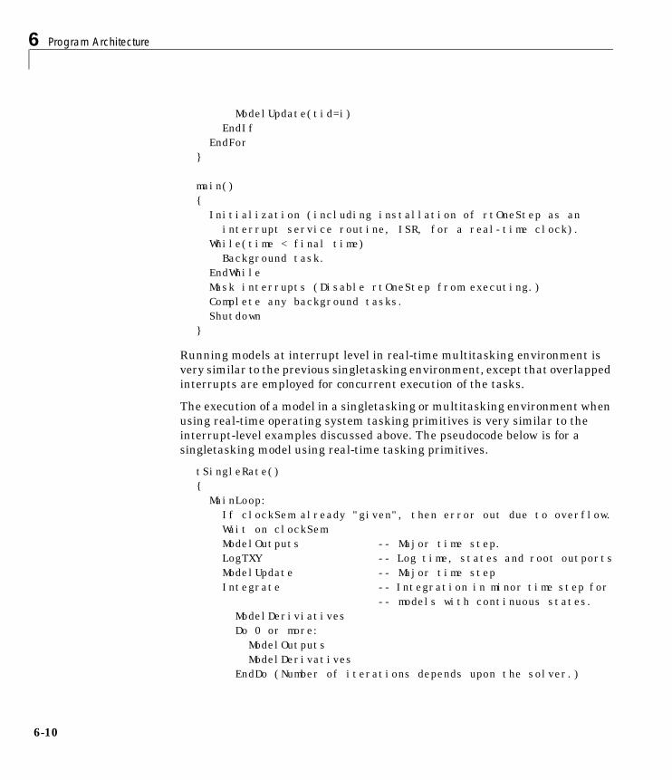
6 Program Architecture
6-10
ModelUpdate(tid=i)EndIf
EndFor}
main(){Initialization (including installation of rtOneStep as an interrupt service routine, ISR, for a real-time clock).
While(time < final time)Background task.
EndWhileMask interrupts (Disable rtOneStep from executing.) Complete any background tasks.Shutdown
}
Running models at interrupt level in real-time multitasking environment isvery similar to the previous singletasking environment, except that overlappedinterrupts are employed for concurrent execution of the tasks.
The execution of a model in a singletasking or multitasking environment whenusing real-time operating system tasking primitives is very similar to theinterrupt-level examples discussed above. The pseudocode below is for asingletasking model using real-time tasking primitives.
tSingleRate(){MainLoop:If clockSem already "given", then error out due to overflow.Wait on clockSemModelOutputs -- Major time step.LogTXY -- Log time, states and root outportsModelUpdate -- Major time stepIntegrate -- Integration in minor time step for
-- models with continuous states.ModelDeriviativesDo 0 or more:
ModelOutputsModelDerivatives
EndDo (Number of iterations depends upon the solver.)
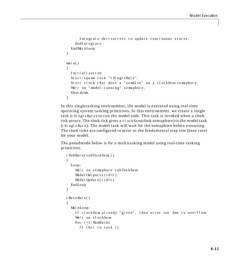
Model Execution
6-11
Integrate derivatives to update continuous states.EndIntegrate
EndMainLoop}
main(){
InitializationStart/spawn task "tSingleRate".Start clock that does a "semGive" on a clockSem semaphore.Wait on "model-running" semaphore.Shutdown
}
In this singletasking environment, the model is executed using real-timeoperating system tasking primitives. In this environment, we create a singletask (tSingleRate) to run the model code. This task is invoked when a clocktick occurs. The clock tick gives a clockSem (clock semaphore) to the model task(tSingleRate). The model task will wait for the semaphore before executing.The clock ticks are configured to occur at the fundamental step size (base rate)for your model.
The pseudocode below is for a multitasking model using real-time taskingprimitives.
tSubRate(subTaskSem,i){
Loop:Wait on semaphore subTaskSem.ModelOutputs(tid=i)ModelUpdate(tid=i)
EndLoop}
tBaseRate(){
MainLoop:If clockSem already "given", then error out due to overflow.Wait on clockSemFor i=1:NumTasksIf (hit in task i)
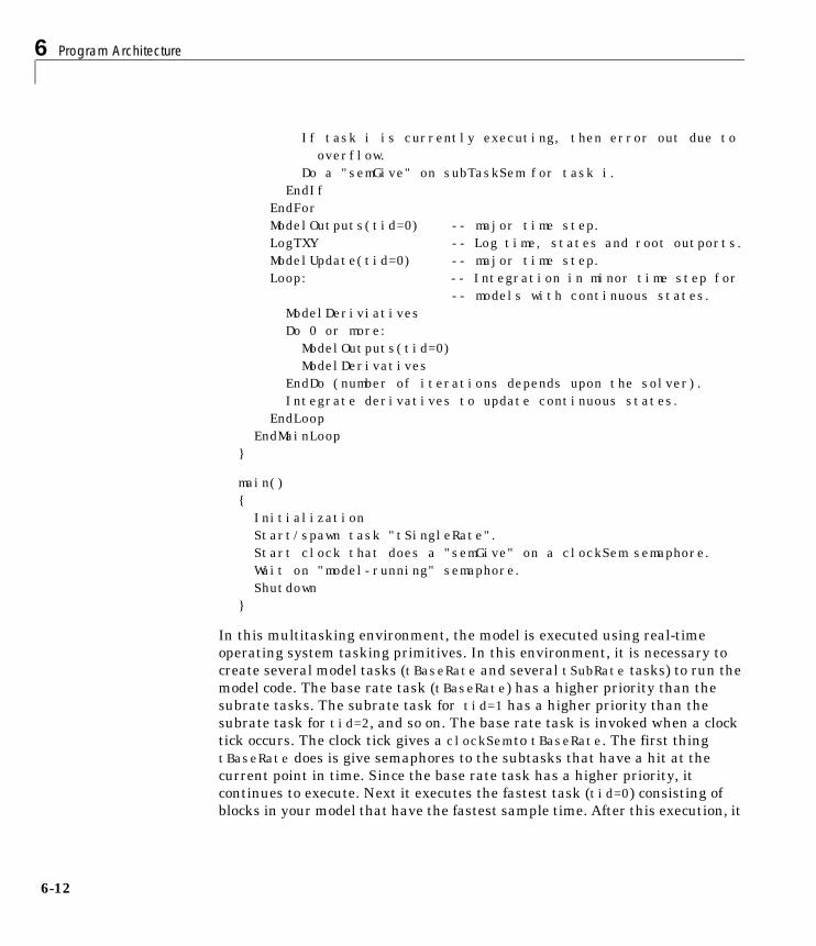
6 Program Architecture
6-12
If task i is currently executing, then error out due to overflow.
Do a "semGive" on subTaskSem for task i.EndIf
EndForModelOutputs(tid=0) -- major time step.LogTXY -- Log time, states and root outports.ModelUpdate(tid=0) -- major time step.Loop: -- Integration in minor time step for
-- models with continuous states.ModelDeriviativesDo 0 or more:
ModelOutputs(tid=0)ModelDerivatives
EndDo (number of iterations depends upon the solver).Integrate derivatives to update continuous states.
EndLoopEndMainLoop
}
main(){InitializationStart/spawn task "tSingleRate".Start clock that does a "semGive" on a clockSem semaphore.Wait on "model-running" semaphore.Shutdown
}
In this multitasking environment, the model is executed using real-timeoperating system tasking primitives. In this environment, it is necessary tocreate several model tasks (tBaseRate and several tSubRate tasks) to run themodel code. The base rate task (tBaseRate) has a higher priority than thesubrate tasks. The subrate task for tid=1 has a higher priority than thesubrate task for tid=2, and so on. The base rate task is invoked when a clocktick occurs. The clock tick gives a clockSem to tBaseRate. The first thingtBaseRate does is give semaphores to the subtasks that have a hit at thecurrent point in time. Since the base rate task has a higher priority, itcontinues to execute. Next it executes the fastest task (tid=0) consisting ofblocks in your model that have the fastest sample time. After this execution, it
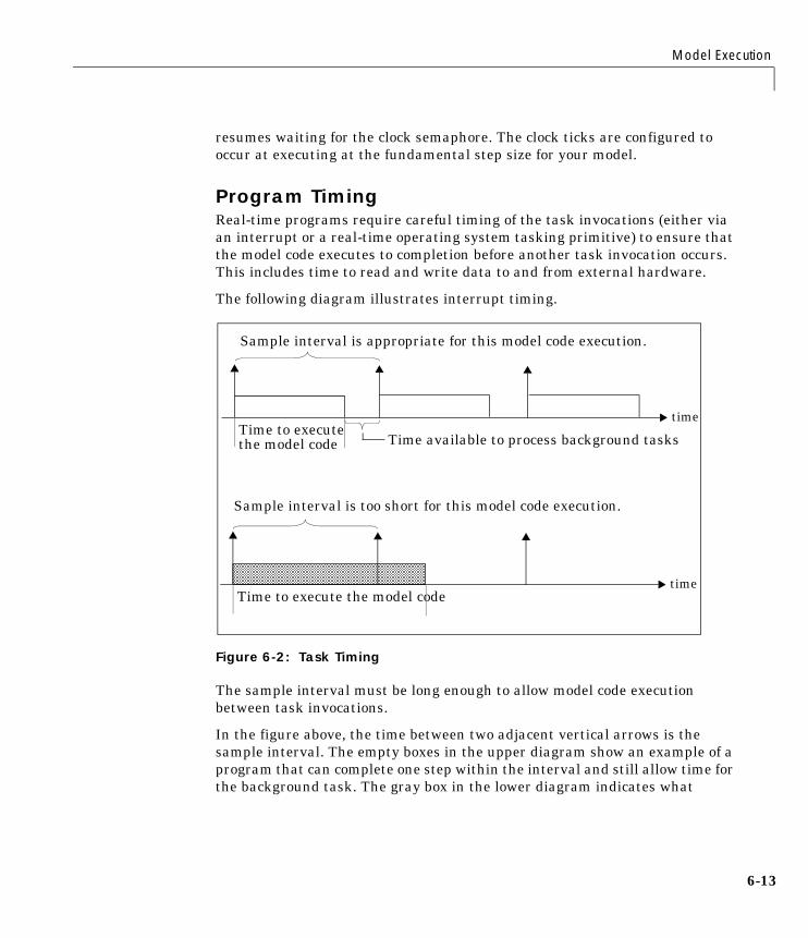
Model Execution
6-13
resumes waiting for the clock semaphore. The clock ticks are configured tooccur at executing at the fundamental step size for your model.
Program TimingReal-time programs require careful timing of the task invocations (either viaan interrupt or a real-time operating system tasking primitive) to ensure thatthe model code executes to completion before another task invocation occurs.This includes time to read and write data to and from external hardware.
The following diagram illustrates interrupt timing.
Figure 6-2: Task Timing
The sample interval must be long enough to allow model code executionbetween task invocations.
In the figure above, the time between two adjacent vertical arrows is thesample interval. The empty boxes in the upper diagram show an example of aprogram that can complete one step within the interval and still allow time forthe background task. The gray box in the lower diagram indicates what
timeTime to execute
Time available to process background tasksthe model code
Sample interval is appropriate for this model code execution.
timeTime to execute the model code
Sample interval is too short for this model code execution.
6 Program Architecture
6-14
happens if the sample interval is too short. Another task invocation occursbefore the task is complete. Such timing results in an execution error.
Note also that, if the real-time program is designed to run forever (i.e., the finaltime is 0 or infinite so the while loop never exits), then the shutdown code neverexecutes.
Program ExecutionAs the previous section indicates, a real-time program may not require 100% ofthe CPU’s time. This provides an opportunity to run background tasks duringthe free time.
Background tasks include operations like writing data to a buffer or file,allowing access to program data by third-party data monitoring tools, or usingSimulink external mode to update program parameters.
It is important, however, that the program be able to preempt the backgroundtask at the appropriate time to ensure real-time execution of the model code.
The way the program manages tasks depends on capabilities of theenvironment in which it operates.
External Mode CommunicationExternal mode allows communication between the Simulink block diagramand the stand-alone program that is built from the generated code. In thismode, the real-time program functions as an interprocess communicationserver, responding to requests from Simulink.
Data Logging In Single-and Multitasking Model ExecutionThe Real-Time Workshop data-logging features, described in “Workspace I/OOptions and Data Logging” in Chapter 3, enable you to save system states,outputs, and time to a MAT-file at the completion of the model execution. TheLogTXY function, which performs data logging, operates differently insingletasking and multitasking environments.
If you examine how LogTXY is called in the singletasking and multitaskingenvironments, you will notice that for singletasking LogTXY is called afterModelOutputs. During this ModelOutputs call, all blocks that have a hit at timet are executed, whereas in multitasking, LogTXY is called after

Model Execution
6-15
ModelOutputs(tid=0) that executes only the blocks that have a hit at time tand that have a task identifier of 0. This results in differences in the loggedvalues between singletasking and multitasking logging. Specifically, considera model with two sample times, the faster sample time having a period of 1.0second and the slower sample time having a period of 10.0 seconds. At time t =k*10, k=0,1,2... both the fast (tid=0) and slow (tid=1) blocks have a hit. Whenexecuting in multitasking mode, when LogTXY is called, the slow blocks willhave a hit, but the previous value will be logged, whereas in singletasking thecurrent value will be logged.
Another difference occurs when logging data in an enabled subsystem.Consider an enabled subsystem that has a slow signal driving the enable portand fast blocks within the enabled subsystem. In this case, the evaluation ofthe enable signal occurs in a slow task and the fast blocks will see a delay ofone sample period, thus the logged values will show these differences.
To summarize differences in logged data between singletasking andmultitasking, differences will be seen when:
• Any root outport block has a sample time that is slower than the fastestsample time
• Any block with states has a sample time that is slower than the fastestsample time
• Any block in an enabled subsystem where the signal driving the enable portis slower than the rate of the blocks in the enabled subsystem
For the first two cases, even though the logged values are different betweensingletasking and multitasking, the model results are not different. The onlyreal difference is where (at what point in time) the logging is done. The third(enabled subsystem) case results in a delay that can be seen in a real-timeenvironment.
Rapid Prototyping and EmbeddedModel Execution DifferencesThe rapid prototyping program framework provides a common applicationprogramming interface (API) that does not change between model definitions.
The Real-Time Workshop Embedded Coder provides a different frameworkthat we will refer to as the embedded program framework. The embeddedprogram framework provides a optimized API that is tailored to your model. It
6 Program Architecture
6-16
is intended that when you use the embedded style of generated code, you aremodeling how you would like your code to execute in your embedded system.Therefore, the definitions defined in your model should be specific to yourembedded targets. Items such as the model name, parameter, and signalstorage class are included as part of the API for the embedded style of code.
The single largest difference between the rapid prototyping and embeddedstyle of generated code is that the embedded code does not contain theSimStruct data structure. The SimStruct defines a common API that the rapidprototyping style of generated code relies heavily on. However, the SimStructdata structure supports many options and therefore consumes memory that isnot needed in an embedded application.
Another major difference between the rapid prototyping and embedded style ofgenerated code is that the latter contains fewer entry-point functions. Theembedded style of code can be configured to have only one run-time functionmodel_step. You can define a single run-time function because the embeddedtarget:
• Can only be used with models that do not have continuous sample time (andtherefore no continuous states)
• Requires that all S-functions must be inlined with the Target LanguageCompiler, which means that they do not access the SimStruct data structure
Thus, when looking at the model execution pseudocode presented earlier in thischapter, you can eliminate the Loop...EndLoop statements, and group theModelOutputs, LogTXY, and ModelUpdate into a single statement, model_step.
For a detailed discussion of how generated embedded code executes, see“Program Execution” on page 9-9.
Rapid Prototyping Model FunctionsThe rapid prototyping code defines the following functions that interface withthe run-time interface:
• Model() — The model registration function. This function for initializes thework areas (e.g., allocating and setting pointers to various data structures)needed by the model. The model registration function calls theMdlInitializeSizes and MdlInitializeSampleTimes functions. These twofunctions are very similar to the S-function mdlInitializeSizes andmdlInitializeSampleTimes methods.
Model Execution
6-17
• MdlStart(void) — After the model registration functions,MdlInitializeSizes and MdlInitializeSampleTimes execute, the run-timeinterface starts execution by calling MdlStart. This routine is called once atstartup.
The function MdlStart has four basic sections:
- Code to initialize the states for each block in the root model that has states.A subroutine call is made to the “initialize states” routine of conditionallyexecuted subsystems.
- Code generated by the one-time initialization (start) function for eachblock in the model.
- Code to enable the blocks in the root model that have enable methods, andthe blocks inside triggered or function-call subsystems residing in the rootmodel. Simulink blocks can have enable and disable methods. An enablemethod is called just before a block starts executing, and the disablemethod is called just after the block stops executing.
- Code for each block in the model that has a constant sample time.
• MdlOutputs(int_T tid) — MdlOutputs updates the output of blocks atappropriate times. The tid (task identifier) parameter identifies the taskthat in turn maps when to execute blocks based upon their sample time. Thisroutine is invoked by the run-time interface during major and minor timesteps. The major time steps are when the run-time interface is taking anactual time step (i.e., it is time to execute a specific task). If your modelcontains continuous states, the minor time steps will be taken. The minortime steps are when the solver is generating integration stages, which arepoints between major outputs. These integration stages are used to computethe derivatives used in advancing the continuous states.
• MdlUpdate(int_T tid) — MdlUpdate updates the discrete states and workvector state information (i.e., states that are neither continuous nor discrete)saved in work vectors. The tid (task identifier) parameter identifies the taskthat in turn indicates which sample times are active allowing you toconditionally update states of only active blocks. This routine is invoked bythe run-time interface after the major MdlOutputs has been executed.
• MdlDerivatives(void) — MdlDerivatives returns the block derivatives.This routine is called in minor steps by the solver during its integrationstages. All blocks that have continuous states have an identical number of
6 Program Architecture
6-18
derivatives. These blocks are required to compute the derivatives so that thesolvers can integrate the states.
• MdlTerminate(void) — MdlTerminate contains any block shutdown code.MdlTerminate is called by the run-time interface, as part of the terminationof the real-time program.
The contents of the above functions are directly related to the blocks in yourmodel. A Simulink block can be generalized to the following set of equations.
Output, y, is a function of continuous state, xc, discrete state, xd, and input, u.Each block writes its specific equation in the appropriate section of MdlOutput.
The discrete states, xd, are a function of the current state and input. Each blockthat has a discrete state updates its state in MdlUpdate.
The derivatives, x, are a function of the current input. Each block that hascontinuous states provides its derivatives to the solver (e.g., ode5) inMdlDerivatives. The derivatives are used by the solver to integrate thecontinuous state to produce the next value.
The output, y, is generally written to the block I/O structure. Root-levelOutport blocks write to the external outputs structure. The continuous anddiscrete states are stored in the states structure. The input, u, can originatefrom another block’s output, which is located in the block I/O structure, anexternal input (located in the external inputs structure), or a state. Thesestructures are defined in the model.h file that the Real-Time Workshopgenerates.
y f0 t x, c xd u, ,( )=
xd 1+ fu t x, d u,( )=
x· fd t xc u, ,( )=
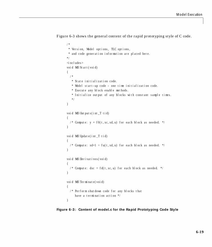
Model Execution
6-19
Figure 6-3 shows the general content of the rapid prototyping style of C code.
Figure 6-3: Content of model.c for the Rapid Prototyping Code Style
/** Version, Model options, TLC options,* and code generation information are placed here.*/<includes>void MdlStart(void){
/** State initialization code.* Model start-up code - one time initialization code.* Execute any block enable methods.* Initialize output of any blocks with constant sample times.*/
}
void MdlOutputs(int_T tid){
/* Compute: y = f0(t,xc,xd,u) for each block as needed. */}
void MdlUpdate(int_T tid){
/* Compute: xd+1 = fu(t,xd,u) for each block as needed. */}
void MdlDerivatives(void){
/* Compute: dxc = fd(t,xc,u) for each block as needed. */}
void MdlTerminate(void){
/* Perform shutdown code for any blocks that have a termination action */
}

6 Program Architecture
6-20
Figure 6-4 shows a flow chart describing the execution of the rapid prototypinggenerated code.
Figure 6-4: Rapid Prototyping Execution Flow Chart
Each block places code into specific Mdl routines according to the algorithmthat it is implementing. Blocks have input, output, parameters, and states, aswell as other general items. For example, in general, block inputs and outputsare written to a block I/O structure (rtB). Block inputs can also come from theexternal input structure (rtU) or the state structure when connected to a stateport of an integrator (rtX), or ground (rtGround) if unconnected or grounded.
End
Inte
grat
ion
MdlDerivatives
MdlOutput
MdlStart
Start Execution
MdlOutput
MdlDerivatives
MdlTerminate
Exe
cuti
onL
oop
MdlUpdate
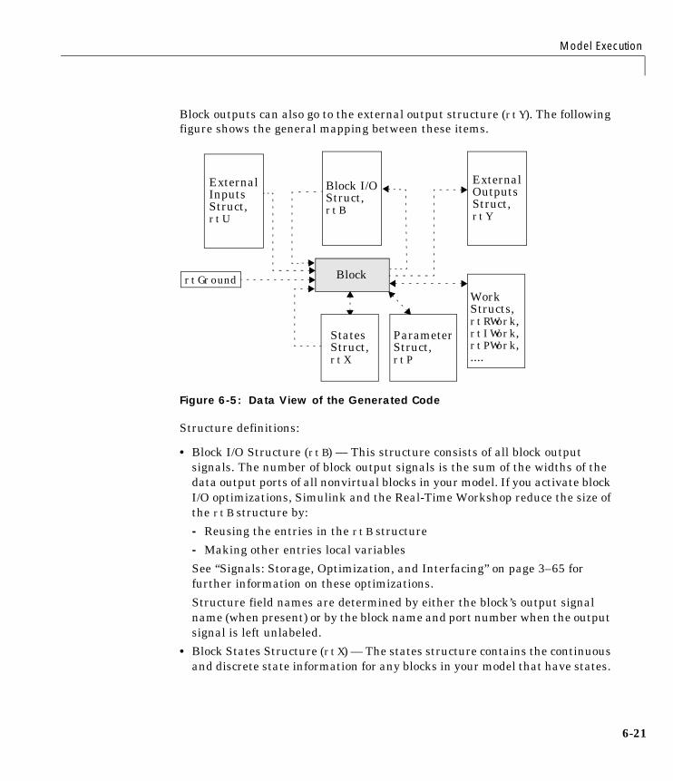
Model Execution
6-21
Block outputs can also go to the external output structure (rtY). The followingfigure shows the general mapping between these items.
Figure 6-5: Data View of the Generated Code
Structure definitions:
• Block I/O Structure (rtB) — This structure consists of all block outputsignals. The number of block output signals is the sum of the widths of thedata output ports of all nonvirtual blocks in your model. If you activate blockI/O optimizations, Simulink and the Real-Time Workshop reduce the size ofthe rtB structure by:
- Reusing the entries in the rtB structure
- Making other entries local variables
See “Signals: Storage, Optimization, and Interfacing” on page 3–65 forfurther information on these optimizations.
Structure field names are determined by either the block’s output signalname (when present) or by the block name and port number when the outputsignal is left unlabeled.
• Block States Structure (rtX) — The states structure contains the continuousand discrete state information for any blocks in your model that have states.
Block
Block I/OStruct,rtB
ExternalOutputsStruct,rtY
ExternalInputsStruct,rtU
rtGround
WorkStructs,rtRWork,rtIWork,rtPWork,....
ParameterStruct,rtP
StatesStruct,rtX
6 Program Architecture
6-22
The states structure has two sections: the first is for the continuous states;the second is for the discrete states.
• Block Parameters Structure (rtP) — The parameters structure contains allblock parameters that can be changed during execution (e.g., the parameterof a Gain block).
• External Inputs Structure (rtU) —The external inputs structure consists ofall root-level Inport block signals. Field names are determined by either theblock’s output signal name, when present, or by the Inport block’s namewhen the output signal is left unlabeled.
• External Outputs Structure (rtY) —The external outputs structure consistsof all root-level Outport blocks. Field names are determined by the root-levelOutport block names in your model.
• Real Work, Integer Work, and Pointer Work Structures (rtRWork, rtIWork,rtPWork) — Blocks may have a need for real, integer, or pointer work areas.For example, the Memory block uses a real work element for each signal.These areas are used to save internal states or similar information.
Embedded Model FunctionsThe Real-Time Workshop Embedded Coder and Ada Coder targets generatethe following functions:
• model_intialize — Performs all model initialization and should be calledonce before you start executing your model.
• If the Single output/update function code generation option is selected,then you will see:
- model_step(int_T tid) — Contains the output and update code for allblocks in your model.
Otherwise you will see:
- model_output(int_T tid) — Contains the output code for all blocks inyour model.
- model_update(int_T tid) — This contains the update code for all blocksin your model.

Model Execution
6-23
• If the Terminate function required code generation option is selected, thenyou will see:
- model_terminate — This contains all model shutdown code and should becalled as part of system shutdown.
See “Code Modules” on page 9–5 and “Program Execution” on page 9–9 forcomplete descriptions of these functions in the context of the Real-TimeWorkshop Embedded Coder.

6 Program Architecture
6-24
Rapid Prototyping Program FrameworkThe code modules generated from a a Simulink model — model.c, model.h, andother files — implement the model’s system equations, contain blockparameters, and perform initialization.
The Real-Time Workshop’s program framework provides the additional sourcecode necessary to build the model code into a complete, stand-alone program.The program framework consists of application modules (files containingsource code to implement required functions) designed for a number ofdifferent programming environments.
The automatic program builder ensures the program is created with the propermodules once you have configured your template makefile.
The application modules and the code generated for a Simulink model areimplemented using a common API. This API defines a data structure (called aSimStruct) that encapsulates all data for your model. Note that the Real-TimeWorkshop Embedded Coder target does not have a SimStruct, but does have acommon calling syntax for model execution.
This API is similar to that of S-functions, with one major exception: the APIassumes that there is only one instance of the model, whereas S-functions canhave multiple instances. The function prototypes also differ from S-functions.
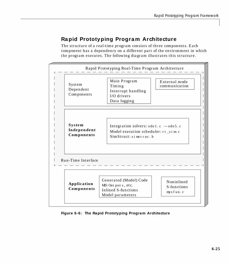
Rapid Prototyping Program Framework
6-25
Rapid Prototyping Program ArchitectureThe structure of a real-time program consists of three components. Eachcomponent has a dependency on a different part of the environment in whichthe program executes. The following diagram illustrates this structure.
Figure 6-6: The Rapid Prototyping Program Architecture
Noninlined
Main Program External modecommunication
Generated (Model) Code
S-functions
Run-Time Interface
TimingInterrupt handlingI/O driversData logging
Model execution scheduler: rt_sim.cSimStruct: simstruc.h
Rapid Prototyping Real-Time Program Architecture
Integration solvers: ode1.c — ode5.c
mysfun.c
SystemDependentComponents
SystemIndependentComponents
ApplicationComponents
MdlOutputs, etc.Inlined S-functionsModel parameters
6 Program Architecture
6-26
The Real-Time Workshop architecture consists of three parts. The first twocomponents, system dependent and independent, together form the run-timeinterface.
This architecture readily adapts to a wide variety of environments by isolatingthe dependencies of each program component. The following sections discusseach component in more detail and include descriptions of the applicationmodules that implement the functions carried out by the system dependent,system independent, and application components.
Rapid Prototyping System Dependent ComponentsThese components contain the program’s main function, which controlsprogram timing, creates tasks, installs interrupt handlers, enables datalogging, and performs error checking.
The way in which application modules implement these operations depends onthe type of computer. This means that, for example, the components used for aDOS-based program perform the same operations, but differ in method ofimplementation from components designed to run under Tornado on a VMEtarget.
The main FunctionThe main function in a C program is the point where execution begins. InReal-Time Workshop application programs, the main function must performcertain operations. These operations can be grouped into three categories:initialization, model execution, and program termination.
Initialization
• Initialize special numeric parameters: rtInf, rtMinusInf, and rtNaN. Theseare variables that the model code can use.
• Call the model registration function to get a pointer to the SimStruct. Themodel registration function has the same name as your model. It isresponsible for initializing SimStruct fields and any S-functions in yourmodel.
• Initialize the model size information in the SimStruct. This is done by callingMdlInitializeSizes.
• Initialize a vector of sample times and offsets (for systems with multiplesample rates). This is done by calling MdlInitializeSampleTimes.
Rapid Prototyping Program Framework
6-27
• Get the model ready for execution by calling MdlStart, which initializesstates and similar items.
• Set up the timer to control execution of the model.
• Define background tasks and enable data logging, if selected.
Model Execution
• Execute a background task, for example, communicate with the host duringexternal mode simulation or introduce a wait state until the next sampleinterval.
• Execute model (initiated by interrupt).
• Log data to buffer (if data logging is used).
• Return from interrupt.
Program Termination• Call a function to terminate the program if it is designed to run for a finite
time — destroy the SimStruct, deallocate memory, and write data to a file.
Rapid Prototyping Application Modules for System Dependent ComponentsThe application modules contained in the system dependent componentsgenerally include a main module such as rt_main.c containing the main entrypoint for C. There may also be additional application modules for such thingsas I/O support and timer handling.
Rapid Prototyping System Independent ComponentsThese components are collectively called system independent because allenvironments use the same application modules to implement theseoperations. This section steps through the model code (and if the model hascontinuous states, calls one of the numerical integration routines). This sectionalso includes the code that defines, creates, and destroys the Simulink datastructure (SimStruct). The model code and all S-functions included in theprogram define their own SimStruct.
The model code execution driver calls the functions in the model code tocompute the model outputs, update the discrete states, integrate the
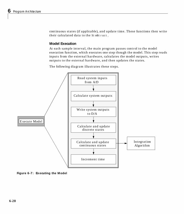
6 Program Architecture
6-28
continuous states (if applicable), and update time. These functions then writetheir calculated data to the SimStruct.
Model ExecutionAt each sample interval, the main program passes control to the modelexecution function, which executes one step though the model. This step readsinputs from the external hardware, calculates the model outputs, writesoutputs to the external hardware, and then updates the states.
The following diagram illustrates these steps.
Figure 6-7: Executing the Model
Read system inputsfrom A/D
Calculate system outputs
Write system outputsto D/A
Calculate and updatediscrete states
Calculate and updatecontinuous states
Increment time
IntegrationAlgorithm
Execute Model

Rapid Prototyping Program Framework
6-29
Note that this scheme writes the system outputs to the hardware before thestates are updated. Separating the state update from the output calculationminimizes the time between the input and output operations.
Integration of Continuous States The real-time program calculates the next values for the continuous statesbased on the derivative vector, dx/dt, for the current values of the inputs andthe state vector.
These derivatives are then used to calculate the next value of the states usinga state-update equation. This is the state-update equation for the first orderEuler method (ode1)
where h is the step size of the simulation, x represents the state vector, anddx/dt is the vector of derivatives. Other algorithms may make several calls tothe output and derivative routines to produce more accurate estimates.
Note, however, that real-time programs use a fixed-step size since it isnecessary to guarantee the completion of all tasks within a given amount oftime. This means that, while you should use higher order integration methodsfor models with widely varying dynamics, the higher order methods requireadditional computation time. In turn, the additional computation time mayforce you to use a larger step size, which can diminish the accuracy increaseinitially sought from the higher order integration method.
Generally, the stiffer the equations, (i.e., the more dynamics in the system withwidely varying time constants), the higher the order of the method that youmust use.
In practice, the simulation of very stiff equations is impractical for real-timepurposes except at very low sample rates. You should test fixed-step sizeintegration in Simulink to check stability and accuracy before implementingthe model for use in real-time programs.
For linear systems, it is more practical to convert the model that you aresimulating to a discrete time version, for instance, using the c2d function in theControl System Toolbox.
x x dxdt-------h+=
6 Program Architecture
6-30
Application Modules for System Independent ComponentsThe system independent components include these modules:
• ode1.c, ode2.c, ode3.c, ode4.c, ode5.c — These modules implement theintegration algorithms supported for real-time applications. See theSimulink documentation for more information about these fixed-stepsolvers.
• rt_sim.c — Performs the activities necessary for one time step of the model.It calls the model function to calculate system outputs and then updates thediscrete and continuous states.
• simstruc.h — Contains actual definition of the Simulink data structure andthe definition of the SimStruct access macros.
• simstruc_types.h — Contains definitions of various events, includingsubsystem enable/disable and zero crossings. It also defines data loggingvariables.
The system independent components also include code that defines, creates,and destroys the Simulink data structure (SimStruct). The model code and allS-functions included in the program define their own SimStruct.
The SimStruct data structure encapsulates all the data relating to the modelor S-function, including block parameters and outputs. See WritingS-Functions for more information about the SimStruct.
Rapid Prototyping Application ComponentsThe application components contain the generated code for the Simulinkmodel, including the code for any S-functions in the model. This code is referredto as the model code because these functions implement the Simulink model.
However, the generated code contains more than just functions to execute themodel (as described in the previous section). There are also functions toperform initialization, facilitate data access, and complete tasks beforeprogram termination. To perform these operations, the generated code mustdefine functions that:
• Create the SimStruct.
• Initialize model size information in the SimStruct.
• Initialize a vector of sample times and sample time offsets and store thisvector in the SimStruct.
Rapid Prototyping Program Framework
6-31
• Store the values of the block initial conditions and program parameters inthe SimStruct.
• Compute the block and system outputs.
• Update the discrete state vector.
• Compute derivatives for continuous models.
• Perform an orderly termination at the end of the program (when the currenttime equals the final time, if a final time is specified).
• Collect block and scope data for data logging (either with the Real-TimeWorkshop or third-party tools).
The SimStruct Data StructureThe generated code includes the file simstruc.h, which contains the definitionof the SimStruct data structure. Each instance of a model (or an S-function) inthe program creates its own SimStruct, which it uses for reading and writingdata.
All functions in the generated code are public. For this reason, there can be onlyone instance of a model in a real-time program. This function, which alwayshas the same name as the model, is called during program initialization toreturn a pointer to the SimStruct and initialize any S-functions.
Rapid Prototyping Model Code FunctionsThe functions defined by the model code are called at various stages of programexecution (i.e., initialization, model execution, or program termination).
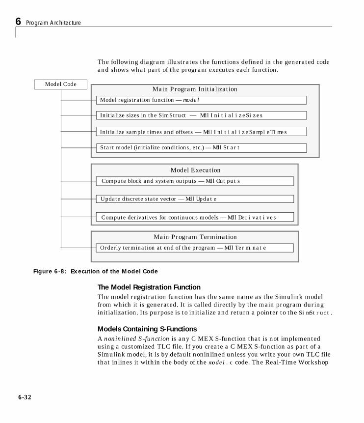
6 Program Architecture
6-32
The following diagram illustrates the functions defined in the generated codeand shows what part of the program executes each function.
Figure 6-8: Execution of the Model Code
The Model Registration FunctionThe model registration function has the same name as the Simulink modelfrom which it is generated. It is called directly by the main program duringinitialization. Its purpose is to initialize and return a pointer to the SimStruct.
Models Containing S-Functions A noninlined S-function is any C MEX S-function that is not implementedusing a customized TLC file. If you create a C MEX S-function as part of aSimulink model, it is by default noninlined unless you write your own TLC filethat inlines it within the body of the model.c code. The Real-Time Workshop
Main Program Termination
Model registration function — model
Update discrete state vector — MdlUpdate
Initialize sample times and offsets — MdlInitializeSampleTimes
Compute block and system outputs — MdlOutputs
Orderly termination at end of the program — MdlTerminate
Compute derivatives for continuous models — MdlDerivatives
Initialize sizes in the SimStruct — MdlInitializeSizes
Model Execution
Main Program InitializationModel Code
Start model (initialize conditions, etc.) — MdlStart
Rapid Prototyping Program Framework
6-33
automatically incorporates your non-inlined C code S-functions into theprogram if they adhere to the S-function API described in the Simulinkdocumentation.
This format defines functions and a SimStruct that are local to the S-function.This allows you to have multiple instances of the S-function in the model. Themodel’s SimStruct contains a pointer to each S-function’s SimStruct.
Code Generation and S-FunctionsIf a model contains S-functions, the source code for the S-function must be onthe search path the make utility uses to find other source files. The directoriesthat are searched are specified in the template makefile that is used to buildthe program.
S-functions are implemented in a way that is directly analogous to the modelcode. They contain their own public registration function (which is called by thetop-level model code) that initializes static function pointers in its SimStruct.When the top-level model needs to execute the S-function, it does so via thefunction pointers in the S-function’s SimStruct. The S-functions use the sameSimStruct data structure as the generated code; however, there can be morethan one S-function with the same name in your model. This is accomplishedby having function pointers to static functions.
Inlining S-FunctionsYou can incorporate C MEX S-functions, along with the generated code, intothe program executable. You can also write a target file for your C MEXS-function to inline the S-function, thus improving performance by eliminatingfunction calls to the S-function itself. For more information on inliningS-functions, see the Target Language Compiler Reference Guide.
6 Program Architecture
6-34
Application Modules for Application ComponentsWhen the Real-Time Workshop generates code, it produces the following files:
• model.c— The C code generated from the Simulink block diagram. This codeimplements the block diagram’s system equations as well as performinginitialization and updating outputs.
• model.h — Header file containing the block diagram’s simulationparameters, I/O structures, work structures, and other declarations.
• model_export.h — Header file containing declarations of exported signalsand parameters.
These files are named for the Simulink model from which they are generated.
If you have created custom blocks using C MEX S-functions, you need thesource code for these S-functions available during the build process.

Embedded Program Framework
6-35
Embedded Program FrameworkThe Real-Time Workshop Embedded Coder provides a framework forembedded programs. Its architecture is outlined by the following figure.
Figure 6-9: Embedded Program Architecture
Main Program
Generated (Model) Code
Run-time Interface
TimingInterrupt handlingI/O driversData logging
Model execution scheduler: rt_sim.c
Embedded Program Architecture
Integration solvers: ode1.c — ode5.c
SystemDependentComponents
SystemIndependentComponents
ApplicationComponents
MdlOutputs, etc.Inlined S-functionsModel parameters
6 Program Architecture
6-36
Note the similarity between this architecture and the rapid prototypingarchitecture on page 6-25. The main difference is the lack of the SimStructdata structure and the removal of the noninlined S-functions.
Using this figure, you can compare the embedded style of generated code, usedin the Real-Time Workshop Embedded Coder, with the rapid prototyping styleof generated code of the previous section. Most of the rapid prototypingexplanations in the previous section hold for the Real-Time WorkshopEmbedded Coder target. The Real-Time Workshop Embedded Coder targetsimplifies the process of using the generated code in your custom-embeddedapplications by providing a model- specific API and eliminating the SimStruct.This target contains the same conceptual layering as the rapid prototypingtarget, but each layer has been simplified.
For a discussion of the structure of embedded real-time code, see Chapter 9,“Real-Time Workshop Embedded Coder.”
7Models with MultipleSample Rates
Introduction . . . . . . . . . . . . . . . . . . . . 7-2
Single- Versus Multitasking Environments . . . . . . . 7-3Executing Multitasking Models . . . . . . . . . . . . . 7-5Multitasking and Pseudomultitasking . . . . . . . . . . 7-5Building the Program for Multitasking Execution . . . . . 7-8Singletasking . . . . . . . . . . . . . . . . . . . . 7-9Building the Program for Singletasking Execution . . . . . 7-9Model Execution . . . . . . . . . . . . . . . . . . . 7-9Simulating Models with Simulink . . . . . . . . . . . . 7-10Executing Models in Real Time . . . . . . . . . . . . . 7-10
Sample Rate Transitions . . . . . . . . . . . . . . . 7-12Faster to Slower Transitions in Simulink . . . . . . . . . 7-13Faster to Slower Transitions in Real Time . . . . . . . . 7-14Slower to Faster Transitions in Simulink . . . . . . . . . 7-16Slower to Faster Transitions in Real Time . . . . . . . . 7-17

7 Models with Multiple Sample Rates
7-2
IntroductionEvery Simulink block can be classified according to its sample time asconstant, continuous-time, discrete-time, inherited, or variable. Examples ofeach type include:
• Constant — Constant block, Width
• Continuous-time — Integrator, Derivative, Transfer Function
• Discrete-time — Unit Delay, Digital Filter
• Inherited — Gain, Sum, Lookup Table
• Variable — These are S-Function blocks that set their time of next hit basedupon current information. These blocks work only with variable step solvers.
Blocks in the inherited category assume the sample time of the blocks that aredriving them. Every Simulink block therefore has a sample time, whether it isexplicit, as in the case of continuous or discrete blocks (continuous blocks havea sample time of zero), or implicit, as in the case of inherited blocks.
Simulink allows you to create models without any restrictions on connectionsbetween blocks with different sample times. It is therefore possible to haveblocks with differing sample times in a model (a mixed-rate system). A possibleadvantage of employing multiple sample times is improved efficiency whenexecuting in a multitasking real-time environment.
Simulink provides considerable flexibility in building these mixed-ratesystems. However, the same flexibility also allows you to construct models forwhich the code generator cannot generate correct real-time code for executionin a multitasking environment. But to make these models operate correctly inreal time (i.e., give the right answers), you must modify your model. In general,the modifications involve placing Unit Delay and Zero Order Hold blocksbetween blocks that have unequal sample rates. The sections that followdiscuss the issues you must address to use a mixed-rate model successfully ina multitasking environment.
Single- Versus Multitasking Environments
7-3
Single- Versus Multitasking EnvironmentsThere are two basic ways in which you can execute a fixed-step Simulinkmodel: singletasking and multitasking. You use the Solver options pull-downmenu on the Solver page of the Simulation Parameters dialog box to specifyhow to execute your model. The default is auto, which specifies that your modelwill use multitasking if your model contains two or more different rates.Otherwise, it will use singletasking.
Execution of models in a real-time system can be done with the aid of areal-time operating system, or it can be done on a bare-board target, where themodel runs in the context of an interrupt service routine (ISR).
Note that the fact that a system (such as UNIX or Microsoft Windows) ismultitasking does not guarantee that the program can execute in real time.This is because it is not guaranteed that the program can preempt otherprocesses when required.
In DOS, where only one process can exist at any given time, an interruptservice routine (ISR) must perform the steps of saving the processor context,executing the model code, collecting data, and restoring the processor context.
Tornado, on the other hand, provides automatic context switching and taskscheduling. This simplifies the operations performed by the ISR. In this case,the ISR simply enables the model execution task, which is normally blocked.
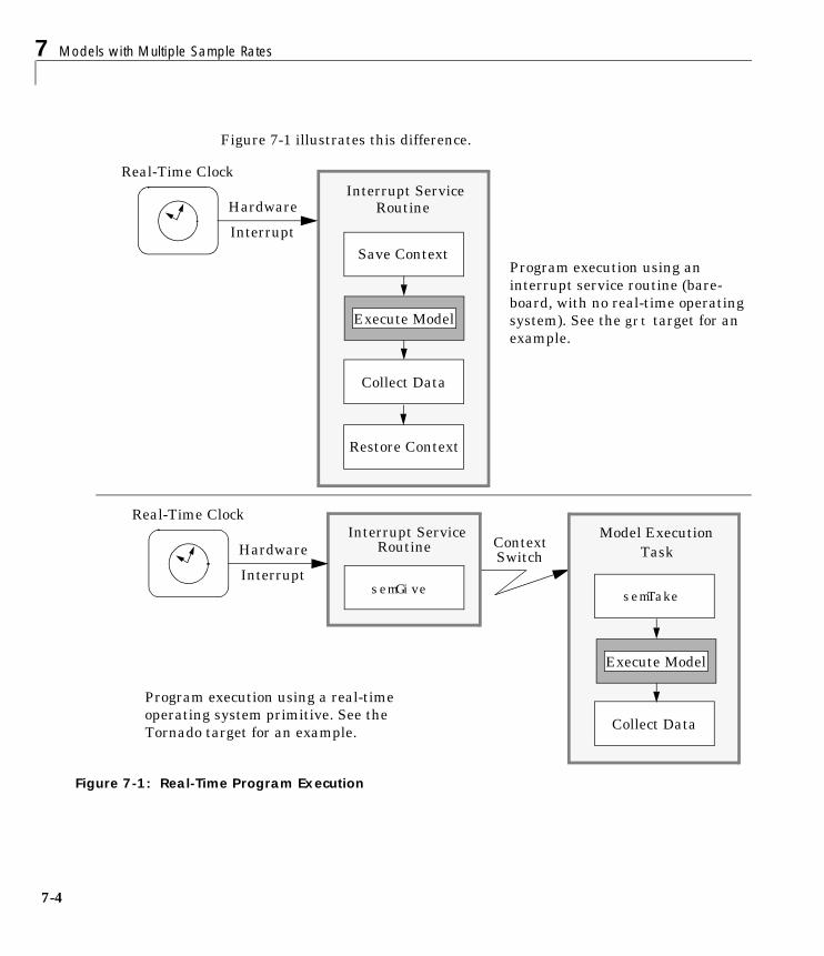
7 Models with Multiple Sample Rates
7-4
Figure 7-1 illustrates this difference.
Figure 7-1: Real-Time Program Execution
Collect Data
Real-Time Clock
semTakesemGive
Interrupt ServiceRoutine
Model ExecutionTask
ContextSwitchHardware
Interrupt
Collect Data
Save Context
Interrupt ServiceRoutine
Real-Time Clock
Hardware
Interrupt
Restore Context
Program execution using a real-time
Program execution using an
Execute Model
Execute Model
interrupt service routine (bare-board, with no real-time operatingsystem). See the grt target for anexample.
operating system primitive. See theTornado target for an example.
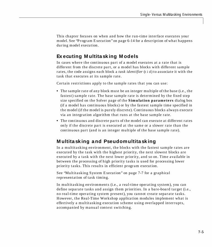
Single- Versus Multitasking Environments
7-5
This chapter focuses on when and how the run-time interface executes yourmodel. See “Program Execution” on page 6-14 for a description of what happensduring model execution.
Executing Multitasking ModelsIn cases where the continuous part of a model executes at a rate that isdifferent from the discrete part, or a model has blocks with different samplerates, the code assigns each block a task identifier (tid) to associate it with thetask that executes at its sample rate.
Certain restrictions apply to the sample rates that you can use:
• The sample rate of any block must be an integer multiple of the base (i.e., thefastest) sample rate. The base sample rate is determined by the fixed stepsize specified on the Solver page of the Simulation parameters dialog box(if a model has continuous blocks) or by the fastest sample time specified inthe model (if the model is purely discrete). Continuous blocks always executevia an integration algorithm that runs at the base sample rate.
• The continuous and discrete parts of the model can execute at different ratesonly if the discrete part is executed at the same or a slower rate than thecontinuous part (and is an integer multiple of the base sample rate).
Multitasking and PseudomultitaskingIn a multitasking environment, the blocks with the fastest sample rates areexecuted by the task with the highest priority, the next slowest blocks areexecuted by a task with the next lower priority, and so on. Time available inbetween the processing of high priority tasks is used for processing lowerpriority tasks. This results in efficient program execution.
See “Multitasking System Execution” on page 7-7 for a graphicalrepresentation of task timing.
In multitasking environments (i.e., a real-time operating system), you candefine separate tasks and assign them priorities. In a bare-board target (i.e.,no real-time operating system present), you cannot create separate tasks.However, the Real-Time Workshop application modules implement what iseffectively a multitasking execution scheme using overlapped interrupts,accompanied by manual context switching.

7 Models with Multiple Sample Rates
7-6
This means an interrupt can occur while another interrupt is currently inprogress. When this happens, the current interrupt is preempted, thefloating-point unit (FPU) context is saved, and the higher priority interruptexecutes its higher priority (i.e., faster sample rate) code. Once complete,control is returned to the preempted ISR.
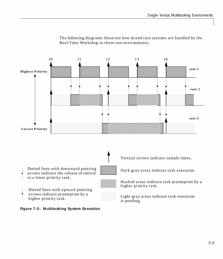
Single- Versus Multitasking Environments
7-7
The following diagrams illustrate how mixed-rate systems are handled by theReal-Time Workshop in these two environments.
Figure 7-2: Multitasking System Execution
Hashed areas indicate task preemption by ahigher priority task.
t0 t1 t2 t3 t4
Lowest Priority
Highest Priority
Vertical arrows indicate sample times.
Dark gray areas indicate task execution.Dotted lines with downward pointing
to a lower priority task.arrows indicate the release of control
Dotted lines with upward pointingarrows indicate preemption by ahigher priority task.
rate 1
rate 2
rate 3
Light gray areas indicate task executionis pending.
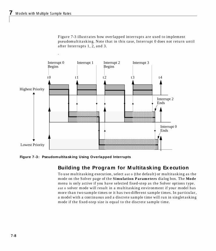
7 Models with Multiple Sample Rates
7-8
Figure 7-3 illustrates how overlapped interrupts are used to implementpseudomultitasking. Note that in this case, Interrupt 0 does not return untilafter Interrupts 1, 2, and 3.
.
Figure 7-3: Pseudomultitasking Using Overlapped Interrupts
Building the Program for Multitasking ExecutionTo use multitasking execution, select auto (the default) or multitasking as themode on the Solver page of the Simulation Parameters dialog box. The Modemenu is only active if you have selected fixed-step as the Solver options type.auto solver mode will result in a multitasking environment if your model hasmore than two sample times or it has two different sample times. In particular,a model with a continuous and a discrete sample time will run in singletaskingmode if the fixed-step size is equal to the discrete sample time.
t0 t1 t2 t3 t4
Lowest Priority
Highest Priority
Interrupt 0Begins
Interrupt 0Ends
Interrupt 2Ends
Interrupt 2Begins
Interrupt 3Interrupt 1
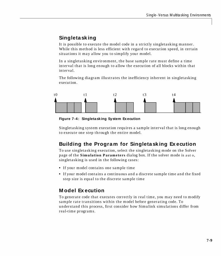
Single- Versus Multitasking Environments
7-9
SingletaskingIt is possible to execute the model code in a strictly singletasking manner.While this method is less efficient with regard to execution speed, in certainsituations it may allow you to simplify your model.
In a singletasking environment, the base sample rate must define a timeinterval that is long enough to allow the execution of all blocks within thatinterval.
The following diagram illustrates the inefficiency inherent in singletaskingexecution.
Figure 7-4: Singletasking System Execution
Singletasking system execution requires a sample interval that is long enoughto execute one step through the entire model.
Building the Program for Singletasking ExecutionTo use singletasking execution, select the singletasking mode on the Solverpage of the Simulation Parameters dialog box. If the solver mode is auto,singletasking is used in the following cases:
• If your model contains one sample time
• If your model contains a continuous and a discrete sample time and the fixedstep size is equal to the discrete sample time
Model ExecutionTo generate code that executes correctly in real time, you may need to modifysample rate transitions within the model before generating code. Tounderstand this process, first consider how Simulink simulations differ fromreal-time programs.
t0 t1 t2 t3 t4

7 Models with Multiple Sample Rates
7-10
Simulating Models with SimulinkBefore Simulink simulates a model, it orders all of the blocks based upon theirtopological dependencies. This includes expanding subsystems into theindividual blocks they contain and flattening the entire model into a single list.Once this step is complete, each block is executed in order.
The key to this process is the proper ordering of blocks. Any block whose outputis directly dependent on its input (i.e., any block with direct feedthrough)cannot execute until the block driving its input has executed.
Some blocks set their outputs based on values acquired in a previous time stepor from initial conditions specified as a block parameter. The output of such ablock is determined by a value stored in memory, which can be updatedindependently of its input. During simulation, all necessary computations areperformed prior to advancing the variable corresponding to time. In essence,this results in all computations occurring instantaneously (i.e., nocomputational delay).
Executing Models in Real TimeA real-time program differs from a Simulink simulation in that the programmust execute the model code synchronously with real time. Every calculationresults in some computational delay. This means the sample intervals cannotbe shortened or lengthened (as they can be in Simulink), which leads to lessefficient execution.
Figure 7-5: Unused Time in Sample Interval
Sample interval t1 cannot be compressed to increase execution speed becauseby definition, sample times are clocked in real time.
Real-Time Workshop application programs are designed to circumvent thispotential inefficiency by using a multitasking scheme. This technique definestasks with different priorities to execute parts of the model code that havedifferent sample rates.
t0 t1 t2
Time
Single- Versus Multitasking Environments
7-11
See “Multitasking and Pseudomultitasking” on page 7–5 for a description ofhow this works. It is important to understand that section before proceedinghere.
Multitasking OperationThe use of multitasking can improve the efficiency of your program if the modelis large and has many blocks executing at each rate. It can also degradeperformance if your model is dominated by a single rate, and only a few blocksexecute at a slower rate. In this situation, the overhead incurred in taskswitching can be greater than the time required to execute the slower blocks.It is more efficient to execute all blocks at the dominant rate.
If you have a model that can benefit from multitasking execution, you mayneed to modify your Simulink model for this scheme to generate correct results.
Singletasking OperationAlternatively, you can run your real-time program in singletasking mode.Singletasking programs require longer sample intervals due to the inherentinefficiency of that mode of execution.

7 Models with Multiple Sample Rates
7-12
Sample Rate TransitionsThere are two possible sample rate transitions that can exist within a model:
• A faster block driving a slower block
• A slower block driving a faster block
In singletasking systems, there are no issues involved with multiple samplerates. In multitasking and pseudomultitasking systems, however, differingsample rates can cause problems. To prevent possible errors in calculated data,you must control model execution at these transitions. In transitioning fromfaster to slower blocks, you must add Zero-Order Hold blocks between fast toslow transitions and set the sample rate of the Zero-Order Hold block to that ofthe slower block.
Figure 7-6: Transitioning from Faster to Slower Blocks (T = sample period)
becomes
Faster SlowerBlockBlock
T = 1 sec T = 2 sec
Faster SlowerBlock
T = 1 sec T = 2 sec
Zero-OrderHoldBlock
T = 2 sec
This diagram
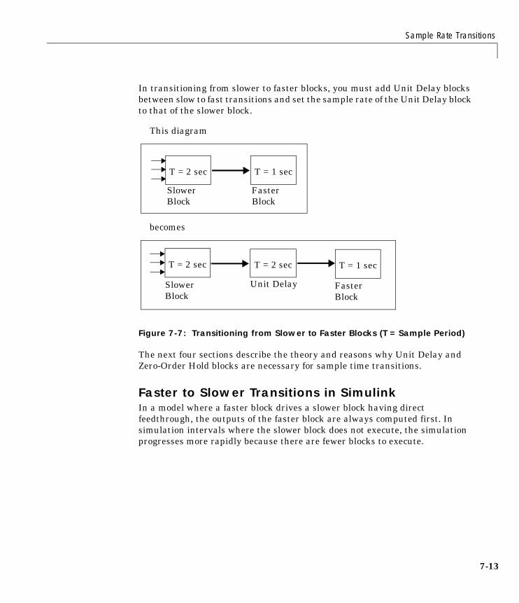
Sample Rate Transitions
7-13
In transitioning from slower to faster blocks, you must add Unit Delay blocksbetween slow to fast transitions and set the sample rate of the Unit Delay blockto that of the slower block.
Figure 7-7: Transitioning from Slower to Faster Blocks (T = Sample Period)
The next four sections describe the theory and reasons why Unit Delay andZero-Order Hold blocks are necessary for sample time transitions.
Faster to Slower Transitions in SimulinkIn a model where a faster block drives a slower block having directfeedthrough, the outputs of the faster block are always computed first. Insimulation intervals where the slower block does not execute, the simulationprogresses more rapidly because there are fewer blocks to execute.
becomes
FasterSlowerBlock Block
T = 1 secT = 2 sec
Slower FasterBlock
T = 2 sec T = 1 sec
Unit DelayBlock
T = 2 sec
This diagram

7 Models with Multiple Sample Rates
7-14
The following diagram illustrates this situation.
Simulink does not execute in real time, which means that it is not bound byreal-time constraints. Simulink waits for, or moves ahead to, whatever tasksare necessary to complete simulation flow. The actual time interval betweensample time steps can vary.
Faster to Slower Transitions in Real TimeIn models where a faster block drives a slower block, you must compensate forthe fact that execution of the slower block may span more than one executionperiod of the faster block. This means that the outputs of the faster block maychange before the slower block has finished computing its outputs. Thefollowing diagram illustrates a situation where this problem arises. Thehashed area indicates times when tasks are preempted by higher prioritybefore completion.
Figure 7-8: Time Overlaps in Faster to Slower Transitions (T=Sample Time)
t0 t1 t2 t3
Time
Faster SlowerBlockBlock
T = 1 sec T = 2 sec
T=2s T=1s T=2s T=1sT=1s T=1s T=2sT=1s
T=2s
T=1s
Time
1 SecTask
2 Sec
1 The faster task (T=1s) completes.
Faster SlowerBlockBlock
T = 1 sec T = 2 sec
T=1s T=1s T=1s
T=2sTask
1
2 3
1
32
2
3
Higher priority preemption occurs.
The slower task (T=2s) resumes and its inputshave changed. This leads to unpredictable results.
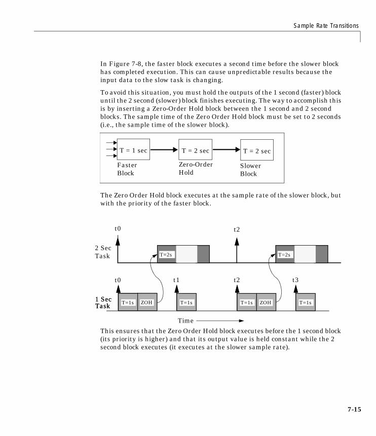
Sample Rate Transitions
7-15
In Figure 7-8, the faster block executes a second time before the slower blockhas completed execution. This can cause unpredictable results because theinput data to the slow task is changing.
To avoid this situation, you must hold the outputs of the 1 second (faster) blockuntil the 2 second (slower) block finishes executing. The way to accomplish thisis by inserting a Zero-Order Hold block between the 1 second and 2 secondblocks. The sample time of the Zero Order Hold block must be set to 2 seconds(i.e., the sample time of the slower block).
The Zero Order Hold block executes at the sample rate of the slower block, butwith the priority of the faster block.
This ensures that the Zero Order Hold block executes before the 1 second block(its priority is higher) and that its output value is held constant while the 2second block executes (it executes at the slower sample rate).
Faster SlowerBlock
T = 1 sec T = 2 sec
Zero-OrderHoldBlock
T = 2 sec
T=1s
T=0.5
ZOH1 SecTask
T=0.5
T=1s T=1s T=1sZOH
t0 t1
T=1s
Time
T=2s
ZOH
t2 t3
1 SecTask
T=2s
T=1s T=1s T=1sZOH
2 SecTask
t0 t2

7 Models with Multiple Sample Rates
7-16
Slower to Faster Transitions in SimulinkIn a model where a slower block drives a faster block, Simulink again computesthe output of the driving block first. During sample intervals where only thefaster block executes, the simulation progresses more rapidly.
The following diagram illustrates the execution sequence.
As you can see from the preceding diagrams, Simulink can simulate modelswith multiple sample rates in an efficient manner. However, Simulink does notoperate in real time.
t0 t1 t2 t3
T=1sT=2s
Time
FasterSlowerBlock Block
T = 1 secT = 2 secT=2sT=1s T=1s T=1s
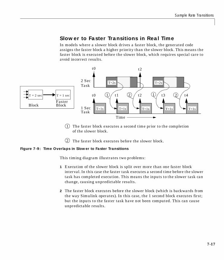
Sample Rate Transitions
7-17
Slower to Faster Transitions in Real TimeIn models where a slower block drives a faster block, the generated codeassigns the faster block a higher priority than the slower block. This means thefaster block is executed before the slower block, which requires special care toavoid incorrect results.
Figure 7-9: Time Overlaps in Slower to Faster Transitions
This timing diagram illustrates two problems:
1 Execution of the slower block is split over more than one faster blockinterval. In this case the faster task executes a second time before the slowertask has completed execution. This means the inputs to the slower task canchange, causing unpredictable results.
2 The faster block executes before the slower block (which is backwards fromthe way Simulink operates). In this case, the 1 second block executes first;but the inputs to the faster task have not been computed. This can causeunpredictable results.
t0 t1
Time
T=2s
t2 t3 t4
1 SecTask
21
1
2
The faster block executes a second time prior to the completionof the slower block.
The faster block executes before the slower block.
FasterBlock Block
T = 1 secT = 2 sec
T=1sT=1s T=1s T=1s T=1s
T=2s2 SecTask
1 2
t0 t2

7 Models with Multiple Sample Rates
7-18
To eliminate these problems, you must insert a Unit Delay block between theslower and faster blocks. The sample rate for a Unit Delay block must be set tothat of the block that is driving it (i.e., the slower block).
The picture below shows the timing sequence that results with the added UnitDelay block.
Three key points about this diagram:
1 Unit delay output runs in 1 second task, but only at its rate (2 seconds). Theoutput of the unit delay block feeds the 1 second task blocks.
2 The unit delay update uses the output of the 2 second task in its update ofits internal state.
3 The unit delay update uses the state of the unit delay in the 1 second task.
Slower FasterBlock
T = 2 sec T = 1 sec
Unit DelayBlock
T = 2 sec
11
t0 t1
1/z
Time
T=1s
t2 t3
1 SecTask
2 Sec
output T=1s T=1s1/z
output1/z
outputT=1s
T=2s1/z
updateTask
11
2
3
T=2s1/z
update

Sample Rate Transitions
7-19
The output portion of a Unit Delay block is executed at the sample rate of theslower block, but with the priority of the faster block. Since a Unit Delay blockdrives the faster block and has effectively the same priority, it is executedbefore the faster block. This solves the first problem.
The second problem is alleviated because the Unit Delay block executes at aslower rate and its output does not change during the computation of the fasterblock it is driving.
Note Inserting a Unit Delay block changes the model. The output of theslower block is now delayed by one time step compared to the output without aUnit Delay block.

7 Models with Multiple Sample Rates
7-20
8Optimizing the Model forCode Generation
Overview . . . . . . . . . . . . . . . . . . . . . . 8-2
General Modeling Techniques . . . . . . . . . . . . 8-3
Block Diagram Performance Tuning . . . . . . . . . . 8-4Look-Up Tables and Polynomials . . . . . . . . . . . . 8-4Accumulators . . . . . . . . . . . . . . . . . . . . 8-15Use of Data Types . . . . . . . . . . . . . . . . . . 8-17
Stateflow Optimizations . . . . . . . . . . . . . . . 8-23
Simulation Parameters . . . . . . . . . . . . . . . 8-24
Compiler Options . . . . . . . . . . . . . . . . . . 8-26
8 Optimizing the Model for Code Generation
8-2
OverviewThere are a number of ways that you can optimize code generated by theReal-Time Workshop from your model, with respect to both memory usage andperformance.
This chapter discusses optimization techniques that are common to all targetconfigurations and code formats. For optimizations specific to a particulartarget configuration, see the chapter relevant to that target.
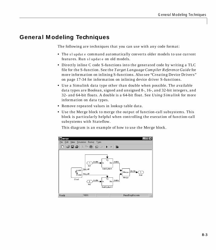
General Modeling Techniques
8-3
General Modeling TechniquesThe following are techniques that you can use with any code format:
• The slupdate command automatically converts older models to use currentfeatures. Run slupdate on old models.
• Directly inline C code S-functions into the generated code by writing a TLCfile for the S-function. See the Target Language Compiler Reference Guide formore information on inlining S-functions. Also see “Creating Device Drivers”on page 17-34 for information on inlining device driver S-functions.
• Use a Simulink data type other than double when possible. The availabledata types are Boolean, signed and unsigned 8-, 16-, and 32-bit integers, and32- and 64-bit floats. A double is a 64-bit float. See Using Simulink for moreinformation on data types.
• Remove repeated values in lookup table data.
• Use the Merge block to merge the output of function-call subsystems. Thisblock is particularly helpful when controlling the execution of function-callsubsystems with Stateflow.
This diagram is an example of how to use the Merge block.
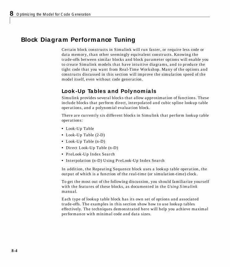
8 Optimizing the Model for Code Generation
8-4
Block Diagram Performance TuningCertain block constructs in Simulink will run faster, or require less code ordata memory, than other seemingly equivalent constructs. Knowing thetrade-offs between similar blocks and block parameter options will enable youto create Simulink models that have intuitive diagrams, and to produce thetight code that you want from Real-Time Workshop. Many of the options andconstructs discussed in this section will improve the simulation speed of themodel itself, even without code generation.
Look-Up Tables and PolynomialsSimulink provides several blocks that allow approximation of functions. Theseinclude blocks that perform direct, interpolated and cubic spline lookup tableoperations, and a polynomial evaluation block.
There are currently six different blocks in Simulink that perform lookup tableoperations:
• Look-Up Table
• Look-Up Table (2-D)
• Look-Up Table (n-D)
• Direct Look-Up Table (n-D)
• PreLook-Up Index Search
• Interpolation (n-D) Using PreLook-Up Index Search
In addition, the Repeating Sequence block uses a lookup table operation, theoutput of which is a function of the real-time (or simulation-time) clock.
To get the most out of the following discussion, you should familiarize yourselfwith the features of these blocks, as documented in the Using Simulinkmanual.
Each type of lookup table block has its own set of options and associatedtrade-offs. The examples in this section show how to use lookup tableseffectively. The techniques demonstrated here will help you achieve maximalperformance with minimal code and data sizes.
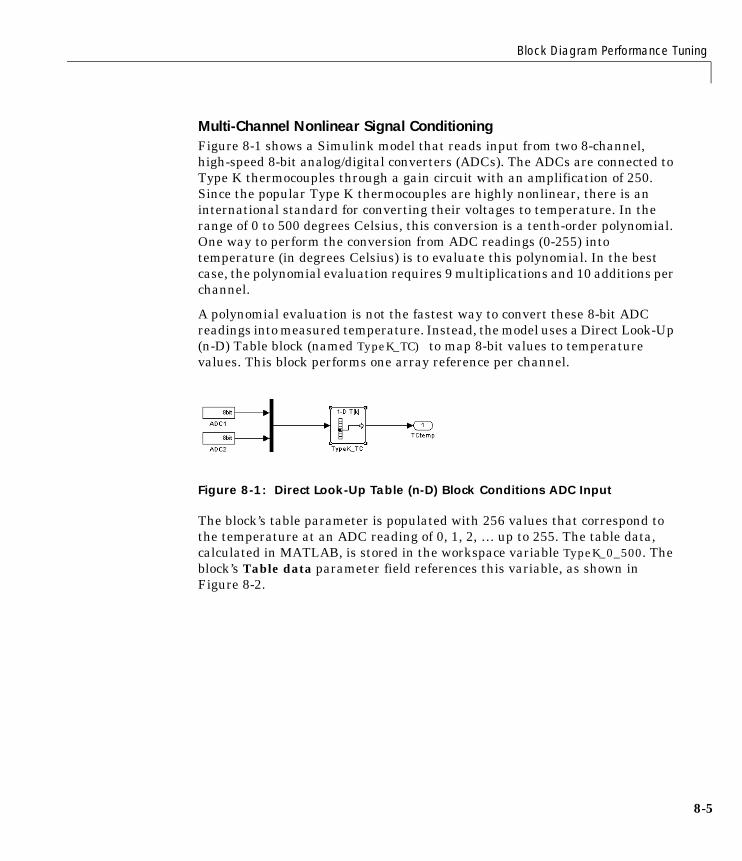
Block Diagram Performance Tuning
8-5
Multi-Channel Nonlinear Signal ConditioningFigure 8-1 shows a Simulink model that reads input from two 8-channel,high-speed 8-bit analog/digital converters (ADCs). The ADCs are connected toType K thermocouples through a gain circuit with an amplification of 250.Since the popular Type K thermocouples are highly nonlinear, there is aninternational standard for converting their voltages to temperature. In therange of 0 to 500 degrees Celsius, this conversion is a tenth-order polynomial.One way to perform the conversion from ADC readings (0-255) intotemperature (in degrees Celsius) is to evaluate this polynomial. In the bestcase, the polynomial evaluation requires 9 multiplications and 10 additions perchannel.
A polynomial evaluation is not the fastest way to convert these 8-bit ADCreadings into measured temperature. Instead, the model uses a Direct Look-Up(n-D) Table block (named TypeK_TC) to map 8-bit values to temperaturevalues. This block performs one array reference per channel.
Figure 8-1: Direct Look-Up Table (n-D) Block Conditions ADC Input
The block’s table parameter is populated with 256 values that correspond tothe temperature at an ADC reading of 0, 1, 2, … up to 255. The table data,calculated in MATLAB, is stored in the workspace variable TypeK_0_500. Theblock’s Table data parameter field references this variable, as shown inFigure 8-2.
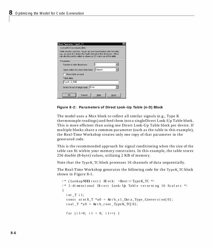
8 Optimizing the Model for Code Generation
8-6
Figure 8-2: Parameters of Direct Look-Up Table (n-D) Block
The model uses a Mux block to collect all similar signals (e.g., Type Kthermocouple readings) and feed them into a singleDirect Look-Up Table block.This is more efficient than using one Direct Look-Up Table block per device. Ifmultiple blocks share a common parameter (such as the table in this example),the Real-Time Workshop creates only one copy of that parameter in thegenerated code.
This is the recommended approach for signal conditioning when the size of thetable can fit within your memory constraints. In this example, the table stores256 double (8-byte) values, utilizing 2 KB of memory.
Note that the TypeK_TC block processes 16 channels of data sequentially.
The Real-Time Workshop generates the following code for the TypeK_TC blockshown in Figure 8-1.
/* (LookupNDDirect) Block: <Root>/TypeK_TC *//* 1-dimensional Direct Look-Up Table returning 16 Scalars */{ int_T i1; const uint8_T *u0 = &rtb_s1_Data_Type_Conversion[0]; real_T *y0 = &rtb_root_TypeK_TC[0];
for (i1=0; i1 < 8; i1++) {
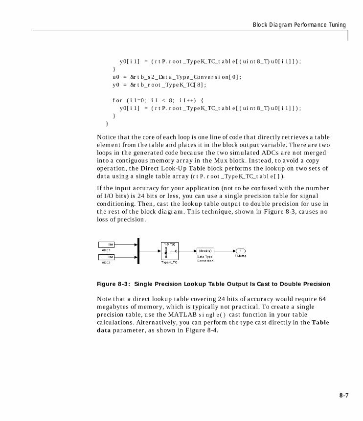
Block Diagram Performance Tuning
8-7
y0[i1] = (rtP.root_TypeK_TC_table[(uint8_T)u0[i1]]); } u0 = &rtb_s2_Data_Type_Conversion[0]; y0 = &rtb_root_TypeK_TC[8];
for (i1=0; i1 < 8; i1++) { y0[i1] = (rtP.root_TypeK_TC_table[(uint8_T)u0[i1]]); }}
Notice that the core of each loop is one line of code that directly retrieves a tableelement from the table and places it in the block output variable. There are twoloops in the generated code because the two simulated ADCs are not mergedinto a contiguous memory array in the Mux block. Instead, to avoid a copyoperation, the Direct Look-Up Table block performs the lookup on two sets ofdata using a single table array (rtP.root_TypeK_TC_table[]).
If the input accuracy for your application (not to be confused with the numberof I/O bits) is 24 bits or less, you can use a single precision table for signalconditioning. Then, cast the lookup table output to double precision for use inthe rest of the block diagram. This technique, shown in Figure 8-3, causes noloss of precision.
Figure 8-3: Single Precision Lookup Table Output Is Cast to Double Precision
Note that a direct lookup table covering 24 bits of accuracy would require 64megabytes of memory, which is typically not practical. To create a singleprecision table, use the MATLAB single() cast function in your tablecalculations. Alternatively, you can perform the type cast directly in the Tabledata parameter, as shown in Figure 8-4.
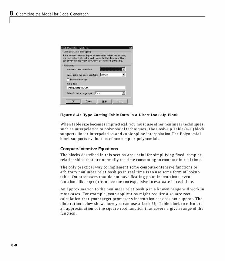
8 Optimizing the Model for Code Generation
8-8
Figure 8-4: Type Casting Table Data in a Direct Look-Up Block
When table size becomes impractical, you must use other nonlinear techniques,such as interpolation or polynomial techniques. The Look-Up Table (n-D) blocksupports linear interpolation and cubic spline interpolation.The Polynomialblock supports evaluation of noncomplex polynomials.
Compute-Intensive EquationsThe blocks described in this section are useful for simplifying fixed, complexrelationships that are normally too time consuming to compute in real time.
The only practical way to implement some compute-intensive functions orarbitrary nonlinear relationships in real time is to use some form of lookuptable. On processors that do not have floating-point instructions, evenfunctions like sqrt() can become too expensive to evaluate in real time.
An approximation to the nonlinear relationship in a known range will work inmost cases. For example, your application might require a square rootcalculation that your target processor’s instruction set does not support. Theillustration below shows how you can use a Look-Up Table block to calculatean approximation of the square root function that covers a given range of thefunction.
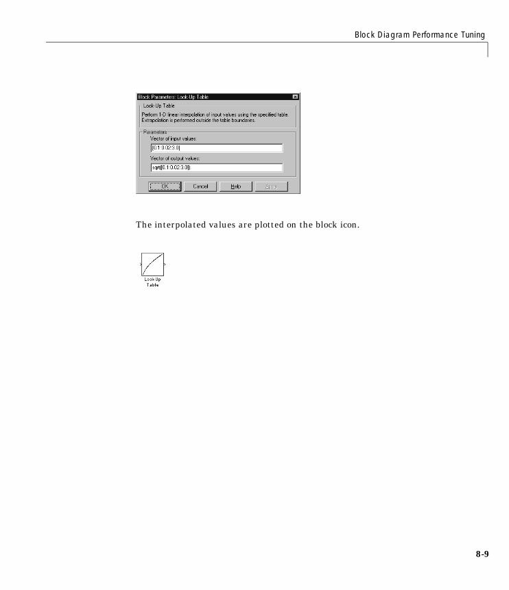
Block Diagram Performance Tuning
8-9
The interpolated values are plotted on the block icon.

8 Optimizing the Model for Code Generation
8-10
For more accuracy on widely spaced points, use a cubic spline interpolation inthe Look-Up Table (n-D) block, as shown below.
Techniques available in Simulink include n-dimensional support for directlookup, linear interpolations in a table, cubic spline interpolations in a table,and 1-D real polynomial evaluation.
The Look-Up Table (n-D) block supports flat interval lookup, linearinterpolation and cubic spline interpolation. Extrapolation for the Look-UpTable (n-D) block can either be disabled (clipping) or enabled for linear orspline extrapolations.
The icons for the Direct Look-Up Table (n-D) and Look-Up Table (n-D) blockschange depending on the type of interpolation selected and the number ofdimensions in the table, as illustrated below.

Block Diagram Performance Tuning
8-11
Tables with Repeated PointsThe Look-Up Table and Look-Up Table (2-D) blocks, shown below, supportlinear interpolation with linear extrapolation. In these blocks, the row andcolumn parameters can have repeated points, allowing pure step behavior to bemixed in with the linear interpolations. Note that this capability is notsupported by the Look-Up Table (n-D) block.
Slowly vs. Rapidly Changing Look-Up Table Block InputsYou can optimize lookup table operations using the Look-Up Table (n-D) blockfor efficiency if you know the input signal’s normal rate of change. Figure 8-5shows the parameters for the Look-Up Table (n-D) block.
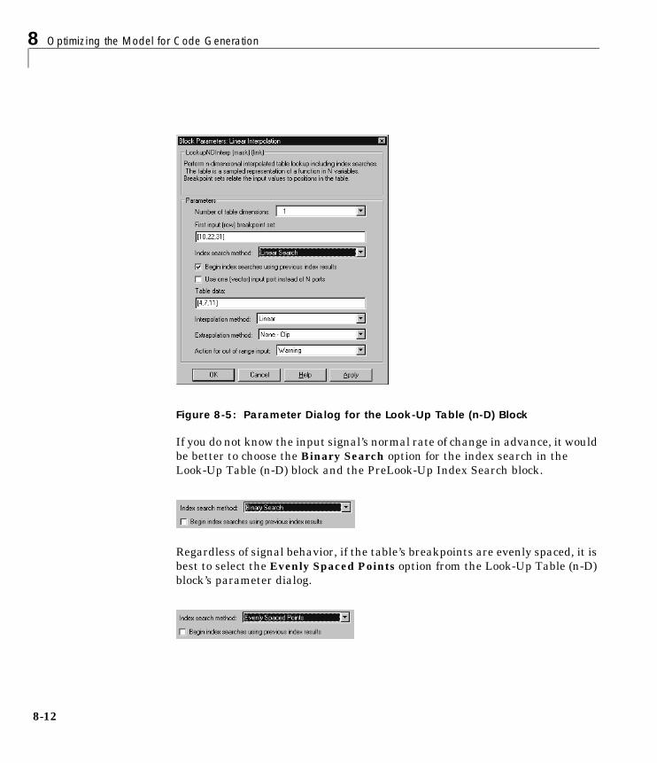
8 Optimizing the Model for Code Generation
8-12
Figure 8-5: Parameter Dialog for the Look-Up Table (n-D) Block
If you do not know the input signal’s normal rate of change in advance, it wouldbe better to choose the Binary Search option for the index search in theLook-Up Table (n-D) block and the PreLook-Up Index Search block.
Regardless of signal behavior, if the table’s breakpoints are evenly spaced, it isbest to select the Evenly Spaced Points option from the Look-Up Table (n-D)block’s parameter dialog.
Block Diagram Performance Tuning
8-13
If the breakpoints are not evenly spaced, first decide which of the following bestdescribes the input signal behavior.
• Behavior 1: The signal stays in a given breakpoint interval from one timestep to the next. When the signal moves to a new interval, it tends to moveto an adjacent interval.
• Behavior 2: The signal has many discontinuities. It jumps around in thetable from one time step to the next, often moving three or more intervals pertime step.
Given behavior 1, the best optimization for a given lookup table is to use theLinear search option and Begin index searches using previous indexresults options, as shown below.
Given behavior 2, the Begin index searches using previous index resultsoption does not necessarily improve performance. Choose the Binary Searchoption, as shown below.
The choice of an index search method can be more complicated for lookup tableoperations of two or more dimensions with linear interpolation. In this case,several signals are input to the table. Some inputs may have evenly spacedpoints, while others may exhibit behavior 1 or behavior 2.
Here it may be best to use PreLook-Up Index Search blocks with differentsearch methods (evenly spaced, linear search or binary search) chosenaccording to the input signal characteristics. The outputs of these search blocksare then connected to an Interpolation (n-D) Using PreLook-Up Index Searchblock, as shown in the block diagram below.
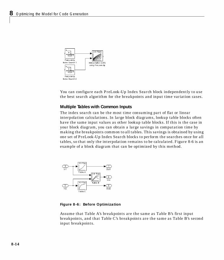
8 Optimizing the Model for Code Generation
8-14
You can configure each PreLook-Up Index Search block independently to usethe best search algorithm for the breakpoints and input time variation cases.
Multiple Tables with Common InputsThe index search can be the most time consuming part of flat or linearinterpolation calculations. In large block diagrams, lookup table blocks oftenhave the same input values as other lookup table blocks. If this is the case inyour block diagram, you can obtain a large savings in computation time bymaking the breakpoints common to all tables. This savings is obtained by usingone set of PreLook-Up Index Search blocks to perform the searches once for alltables, so that only the interpolation remains to be calculated. Figure 8-6 is anexample of a block diagram that can be optimized by this method.
Figure 8-6: Before Optimization
Assume that Table A’s breakpoints are the same as Table B’s first inputbreakpoints, and that Table C’s breakpoints are the same as Table B’s secondinput breakpoints.
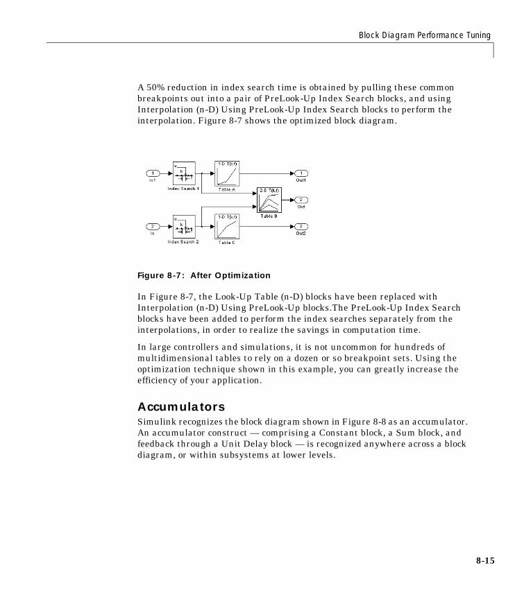
Block Diagram Performance Tuning
8-15
A 50% reduction in index search time is obtained by pulling these commonbreakpoints out into a pair of PreLook-Up Index Search blocks, and usingInterpolation (n-D) Using PreLook-Up Index Search blocks to perform theinterpolation. Figure 8-7 shows the optimized block diagram.
Figure 8-7: After Optimization
In Figure 8-7, the Look-Up Table (n-D) blocks have been replaced withInterpolation (n-D) Using PreLook-Up blocks.The PreLook-Up Index Searchblocks have been added to perform the index searches separately from theinterpolations, in order to realize the savings in computation time.
In large controllers and simulations, it is not uncommon for hundreds ofmultidimensional tables to rely on a dozen or so breakpoint sets. Using theoptimization technique shown in this example, you can greatly increase theefficiency of your application.
AccumulatorsSimulink recognizes the block diagram shown in Figure 8-8 as an accumulator.An accumulator construct — comprising a Constant block, a Sum block, andfeedback through a Unit Delay block — is recognized anywhere across a blockdiagram, or within subsystems at lower levels.
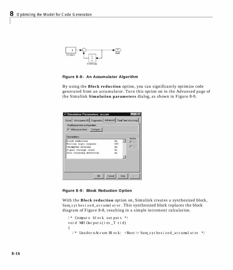
8 Optimizing the Model for Code Generation
8-16
Figure 8-8: An Accumulator Algorithm
By using the Block reduction option, you can significantly optimize codegenerated from an accumulator. Turn this option on in the Advanced page ofthe Simulink Simulation parameters dialog, as shown in Figure 8-9.
Figure 8-9: Block Reduction Option
With the Block reduction option on, Simulink creates a synthesized block,Sum_sythesized_accumulator. This synthesized block replaces the blockdiagram of Figure 8-8, resulting in a simple increment calculation.
/* Compute block outputs */void MdlOutputs(int_T tid){ /* UnadornAccum Block: <Root>/Sum_sythesized_accumulator */
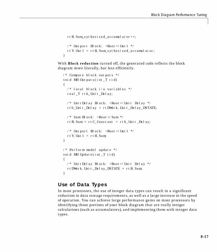
Block Diagram Performance Tuning
8-17
rtB.Sum_sythesized_accumulator++;
/* Outport Block: <Root>/Out1 */ rtY.Out1 = rtB.Sum_sythesized_accumulator;}
With Block reduction turned off, the generated code reflects the blockdiagram more literally, but less efficiently.
/* Compute block outputs */void MdlOutputs(int_T tid){ /* local block i/o variables */ real_T rtb_Unit_Delay;
/* UnitDelay Block: <Root>/Unit Delay */ rtb_Unit_Delay = rtDWork.Unit_Delay_DSTATE;
/* Sum Block: <Root>/Sum */ rtB.Sum = rtC_Constant + rtb_Unit_Delay;
/* Outport Block: <Root>/Out1 */ rtY.Out1 = rtB.Sum;}
/* Perform model update */void MdlUpdate(int_T tid){ /* UnitDelay Block: <Root>/Unit Delay */ rtDWork.Unit_Delay_DSTATE = rtB.Sum;}
Use of Data TypesIn most processors, the use of integer data types can result in a significantreduction in data storage requirements, as well as a large increase in the speedof operation. You can achieve large performance gains on most processors byidentifying those portions of your block diagram that are really integercalculations (such as accumulators), and implementing them with integer datatypes.
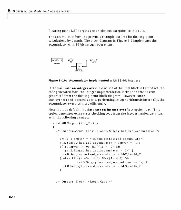
8 Optimizing the Model for Code Generation
8-18
Floating-point DSP targets are an obvious exception to this rule.
The accumulator from the previous example used 64-bit floating-pointcalculations by default. The block diagram in Figure 8-9 implements theaccumulator with 16-bit integer operations.
Figure 8-10: Accumulator Implemented with 16-bit Integers
If the Saturate on integer overflow option of the Sum block is turned off, thecode generated from the integer implementation looks the same as codegenerated from the floating-point block diagram. However, sinceSum_sythesized_accumulator is performing integer arithmetic internally, theaccumulator executes more efficiently.
Note that, by default, the Saturate on integer overflow option is on. Thisoption generates extra error-checking code from the integer implementation,as in the following example.
void MdlOutputs(int_T tid){ /* UnadornAccum Block: <Root>/Sum_sythesized_accumulator */ { int16_T tmpVar = rtB.Sum_sythesized_accumulator; rtB.Sum_sythesized_accumulator = tmpVar + (1); if ((tmpVar >= 0) && ((1) >= 0) && (rtB.Sum_sythesized_accumulator < 0)) { rtB.Sum_sythesized_accumulator = MAX_int16_T; } else if ((tmpVar < 0) && ((1) < 0) && (rtB.Sum_sythesized_accumulator >= 0)) { rtB.Sum_sythesized_accumulator = MIN_int16_T; } }
/* Outport Block: <Root>/Out1 */
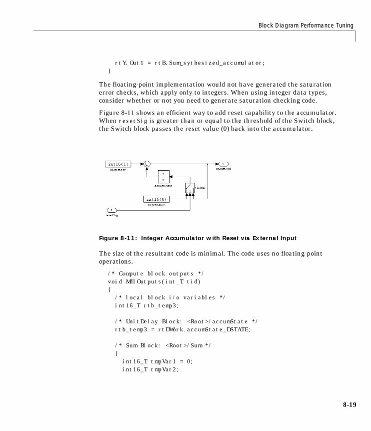
Block Diagram Performance Tuning
8-19
rtY.Out1 = rtB.Sum_sythesized_accumulator;}
The floating-point implementation would not have generated the saturationerror checks, which apply only to integers. When using integer data types,consider whether or not you need to generate saturation checking code.
Figure 8-11 shows an efficient way to add reset capability to the accumulator.When resetSig is greater than or equal to the threshold of the Switch block,the Switch block passes the reset value (0) back into the accumulator.
Figure 8-11: Integer Accumulator with Reset via External Input
The size of the resultant code is minimal. The code uses no floating-pointoperations.
/* Compute block outputs */void MdlOutputs(int_T tid){ /* local block i/o variables */ int16_T rtb_temp3;
/* UnitDelay Block: <Root>/accumState */ rtb_temp3 = rtDWork.accumState_DSTATE;
/* Sum Block: <Root>/Sum */ { int16_T tmpVar1 = 0; int16_T tmpVar2;
8 Optimizing the Model for Code Generation
8-20
/* port 0 */ tmpVar1 = rtC_Increment; /* port 1 */ tmpVar2 = tmpVar1 + rtb_temp3; if ((tmpVar1 >= 0) && (rtb_temp3 >= 0) && (tmpVar2 < 0)) { tmpVar2 = MAX_int16_T; } else if ((tmpVar1 < 0) && (rtb_temp3 < 0) && (tmpVar2 >= 0)) { tmpVar2 = MIN_int16_T; } rtb_temp3 = tmpVar2; }
/* Outport Block: <Root>/accumVal */ rtY.accumVal = rtb_temp3;
/* Switch Block: <Root>/Switch */ if (rtU.resetSig) { rtB.Switch = rtC_ResetValue; } else { rtB.Switch = rtb_temp3; }}
/* Perform model update */void MdlUpdate(int_T tid){ /* UnitDelay Block: <Root>/accumState */ rtDWork.accumState_DSTATE = rtB.Switch;}
In this example, it would be easy to use an input to the system as the resetvalue, rather than a constant.
Generating Pure Integer CodeThe Real-Time Workshop Embedded Coder target provides the Integer codeonly option to ensure that generated code contains no floating-point data oroperations. When this option is selected, an error is raised if any noninteger

Block Diagram Performance Tuning
8-21
data or expressions are encountered during compilation of the model. The errormessage reports the offending blocks and parameters.
If pure integer code generation is important to your design, you should considerusing the Real-Time Workshop Embedded Coder target (or a target of yourown, based on the Real-Time Workshop Embedded Coder target).
To use the Integer code only option, select ERT code generation optionsfrom the Category menu in the Real-Time Workshop page. Then enable theInteger code only option, as shown below.
The Real-Time Workshop Embedded Coder target offers many otheroptimizations. See Chapter 9, “Real-Time Workshop Embedded Coder” forfurther information.
Data Type Optimizations with Fixed-Point Blocksetand StateflowThe Fixed-Point Blockset (a separate product) is designed to deliver the highestlevels of performance for noninteger algorithms on processors lackingfloating-point hardware. The Fixed-Point Blockset’s code generation inReal-Time Workshop implements calculations using a processor’s integeroperations. The code generation strategy maps the integer value set to a rangeof expected real world values to achieve the high efficiency.
8 Optimizing the Model for Code Generation
8-22
Finite-state machine or flowchart constructs can often represent decision logic(or mode logic) efficiently. Stateflow (a separate product) provides thesecapabilities. Stateflow, which is fully integrated into Simulink, supportsinteger data-typed code generation.
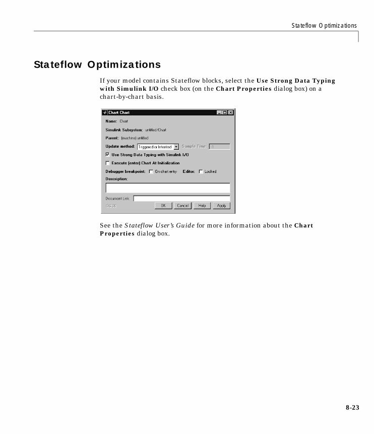
Stateflow Optimizations
8-23
Stateflow OptimizationsIf your model contains Stateflow blocks, select the Use Strong Data Typingwith Simulink I/O check box (on the Chart Properties dialog box) on achart-by-chart basis.
See the Stateflow User’s Guide for more information about the ChartProperties dialog box.

8 Optimizing the Model for Code Generation
8-24
Simulation ParametersOptions on each page of the Simulation Parameters dialog box affect thegenerated code.
Advanced Page
• Turn on the Signal storage reuse option. The directs the Real-TimeWorkshop to store signals in reusable memory locations. It also enables theLocal block outputs option (see “General Code Generation Options” on page8-25).
Disabling Signal storage reuse makes all block outputs global and unique,which in many cases significantly increases RAM and ROM usage.
• Enable strict Boolean type checking by selecting the Boolean logic signalsoption.
Selecting this check box is recommended. Generated code will require lessmemory, because a Boolean signal typically requires one byte of storagewhile a double signal requires eight bytes of storage.
• Select the Inline parameters check box. Inlining parameters reduces globalRAM usage, since parameters are not declared in the global parametersstructure. Note that you can override the inlining of individual parametersby using the Model Parameter Configuration dialog box.
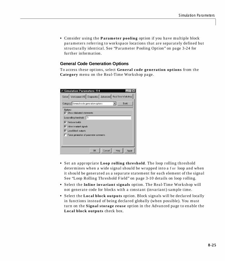
Simulation Parameters
8-25
• Consider using the Parameter pooling option if you have multiple blockparameters referring to workspace locations that are separately defined butstructurally identical. See “Parameter Pooling Option” on page 3-24 forfurther information.
General Code Generation OptionsTo access these options, select General code generation options from theCategory menu on the Real-Time Workshop page.
• Set an appropriate Loop rolling threshold. The loop rolling thresholddetermines when a wide signal should be wrapped into a for loop and whenit should be generated as a separate statement for each element of the signalSee “Loop Rolling Threshold Field” on page 3-10 details on loop rolling.
• Select the Inline invariant signals option. The Real-Time Workshop willnot generate code for blocks with a constant (invariant) sample time.
• Select the Local block outputs option. Block signals will be declared locallyin functions instead of being declared globally (when possible). You mustturn on the Signal storage reuse option in the Advanced page to enable theLocal block outputs check box.
8 Optimizing the Model for Code Generation
8-26
Compiler Options• If you do not require double precision for your application, define real_T asfloat in your template make file, or you can simply specify -DREAL_T=floatafter make_rtw in the Make command field.
• Turn on the optimizations for the compiler (e.g., -O2 for gcc, -Ot for MicrosoftVisual C).
9Real-Time WorkshopEmbedded Coder
Introduction . . . . . . . . . . . . . . . . . . . . 9-2
Data Structures and Code Modules . . . . . . . . . . 9-4Real-Time Object . . . . . . . . . . . . . . . . . . . 9-4Code Modules . . . . . . . . . . . . . . . . . . . . 9-5
Program Execution . . . . . . . . . . . . . . . . . 9-9Overview . . . . . . . . . . . . . . . . . . . . . . 9-9Main Program . . . . . . . . . . . . . . . . . . . . 9-10rt_OneStep . . . . . . . . . . . . . . . . . . . . . 9-11Model Entry Points . . . . . . . . . . . . . . . . . . 9-14
Automatic S-Function Wrapper Generation . . . . . . . 9-17
Optimizing the Generated Code . . . . . . . . . . . . 9-20Basic Code Generation Options . . . . . . . . . . . . . 9-20Generating Code from Subsystems . . . . . . . . . . . 9-22Generating Block Comments . . . . . . . . . . . . . . 9-22Generating a Code Generation Report . . . . . . . . . . 9-23Controlling Stack Space Allocation . . . . . . . . . . . 9-25
Advanced Code Generation Options . . . . . . . . . . 9-27Create Simulink (S-Function) Block . . . . . . . . . . . 9-27Generate HTML Report . . . . . . . . . . . . . . . . 9-27Generate ASAP2 File . . . . . . . . . . . . . . . . . 9-28
Requirements and Restrictions . . . . . . . . . . . . 9-29Unsupported Blocks . . . . . . . . . . . . . . . . . 9-30
System Target File and Template Makefiles . . . . . . . 9-31

9 Real-Time Workshop Embedded Coder
9-2
IntroductionThe Real-Time Workshop Embedded Coder is a separate, add-on product foruse with the Real-Time Workshop.
The Real-Time Workshop Embedded Coder provides a framework for theproduction of code that is optimized for speed, memory usage, and simplicity.The Real-Time Workshop Embedded Coder is intended for use in embeddedsystems.
The Real-Time Workshop Embedded Coder generates code in the Embedded-Cformat. Optimizations inherent in the Embedded-C code format include:
• Use of model-specific real-time object data structure rather than genericSimStruct significantly reduces code size and memory usage.
• Simplified calling interface reduces overhead. Model output and updatefunctions are combined into a single routine.
• In-lined S-functions (required) reduce calling overhead and code size.
• Static memory allocation reduces overhead and promotes deterministicperformance.
The Real-Time Workshop Embedded Coder supports the following keyfeatures:
• Integer only code generation
• Floating-point code generation
• Supports asynchronous interrupt-driven execution of models with eithersingle or multiple sample rates
• Automatic generation of S-function wrappers, allowing you to validate thegenerated code in Simulink (Software-in-the-loop)
• Web-viewable code generation report describes code modules and helps toidentify code generation optimizations relevant to your program
This chapter describes the components of the Real-Time Workshop EmbeddedCoder provided with Real-Time Workshop. It also describes options foroptimizing your generated code, and for automatically generating anS-function wrapper that calls your Real-Time Workshop Embedded Codergenerated code from Simulink. In addition, certain restrictions that apply tothe use of the Real-Time Workshop Embedded Coder are discussed.
9-3
We assume you have read Chapter 6, “Program Architecture” and Chapter 7,“Models with Multiple Sample Rates” in this manual. Those chapters give ageneral overview of the architecture and execution of programs generated byReal-Time Workshop.

9 Real-Time Workshop Embedded Coder
9-4
Data Structures and Code ModulesThis section describes the main data structures of the Real-Time WorkshopEmbedded Coder. It also summarizes the code modules and header files thatmake up a Real-Time Workshop Embedded Coder program, and describeswhere to find them.
Real-Time ObjectUnlike other Real-Time Workshop code formats, Real-Time WorkshopEmbedded Coder generated code does not employ the SimStruct. Instead, theReal-Time Workshop Embedded Coder uses a data structure called thereal-time object. The real-time object, like the SimStruct, contains essentialtiming and scheduling data, as well as model information. The real-time objectis much more compact than the SimStruct, achieving a significant reduction incode size. For example, the real-time object for a single-rate model typicallyrequires 4 bytes.
Note that the real-time object is a model-specific data structure. The real-timeobject for a particular model is defined in model_export.h.
Your code should not reference fields of the real-time object directly. TheReal-Time Workshop provides accessor macros for the real-time object. Thesemacros are defined in matlabroot/rtw/c/ert/ertformat.h. The macros aresyntactically and functionally identical to the SimStruct macros used withother code formats. If you are interfacing your code to a single model, youshould refer to its real-time object generically as RT_OBJ, and use the macros toaccess RT_OBJ, as in the following code fragment.
#include "ertformat.h"const char_T *errStatus = ssGetErrorStatus(RT_OBJ);
For an example of how to interface your code to the real-time objects of morethan one model, see “How to Call the Entry Points Directly” on page 9-16.
The logging object is a subobject of the real-time object. This data structure isused in generated code if the MAT-file logging code generation option isenabled.
Data Structures and Code Modules
9-5
Code ModulesThis section summarizes the code modules and header files of the Real-TimeWorkshop Embedded Coder, and describes where to find them.
Generated Code ModulesThe Real-Time Workshop creates a build directory in your working directory tostore generated source code. The build directory also contains object (.obj)files, a makefile, and other files created during the code generation process.
The default name of the build directory is model_ert_rtw. The build directorycontains the following generated source code modules:
• model.c
model.c defines all entry points to the generated code. These are:- model_step implements all computations required for one time step of
your model.
- model_initialize initializes the real-time object. If logging is enabled, italso initializes the logging object.
- model_terminate performs any cleanup operations required after yourprogram’s main loop has stopped executing. Real-Time Workshopgenerates model_terminate if you select the Terminate functionrequired code generation option (by default, this option is selected).
A standard way to call these entry points is via the macros MODEL_STEP,MODEL_INITIALIZE, and MODEL_TERMINATE. These macros are defined inmatlabroot/rtw/c/ert/ertformat.h. The following code fragmentillustrates their use.#include "ertformat.h"MODEL_INITIALIZE(1);
• model_export.h
model_export.h defines the real-time object and provides a public interfaceto the entry points of the model code. See “How to Call the Entry PointsDirectly” on page 9-16 for an example of how to use this interface.
• model.h
This header defines parameters and data structures private to model.c.
• autobuild.h is generated only for use in test and simulation. This file is notrequired in production environments. You can replace
9 Real-Time Workshop Embedded Coder
9-6
#include "autobuild.h"
with
#include "model_export.h"
Note that the Real-Time Workshop Embedded Coder code generation reportcontains further information about code modules generated during a build.(See “Generating a Code Generation Report” on page 9-23).
Main Program ModuleReal-Time Workshop provides the modulematlabroot/rtw/c/ert/ert_main.c as a template example for developingembedded applications. ert_main.c is not part of the generated code; it isprovided as a basis for your custom modifications, and for use in simulation.
We recommend that you copy ert_main.c to your working directory andrename it to model_ert_main.c before making modifications. The Buildprocess will create model_ert_main.obj in the build directory.
ert_main.c contains:
• rt_OneStep, a timer interrupt service routine (ISR). rt_OneStep callsMODEL_STEP to execute processing for one clock period of the model.
• A skeletal main function. As provided, main is useful in simulation only. Youmust modify main for real-time interrupt-driven execution.
“Program Execution” on page 9-9 contains a detailed discussion of the mainmodule, as well as guidelines for modifying it to meet your requirements.
Utility Header FilesThe following support header files are provided in the directorymatlabroot/rtw/c/ert:
• ertformat.h defines accessor macros for the real-time object, as well as theReal-Time Workshop Embedded Coder entry-point macros.
• tmwtypes.h and simstruc_types.h define Real-Time Workshop data types.These headers are included by ertformat.h.
• log_object.h defines the logging object.
• log_macros.h defines macros that perform logging functions.

Data Structures and Code Modules
9-7
You can include these header files generically for all models. Inclusion of theheader files adds no overhead to the generated code.
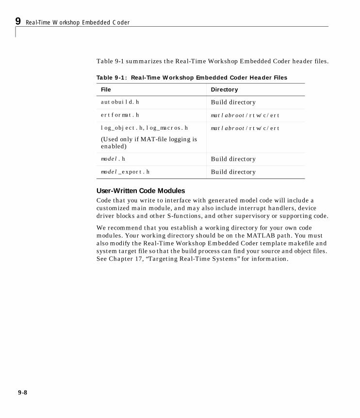
9 Real-Time Workshop Embedded Coder
9-8
Table 9-1 summarizes the Real-Time Workshop Embedded Coder header files.
User-Written Code ModulesCode that you write to interface with generated model code will include acustomized main module, and may also include interrupt handlers, devicedriver blocks and other S-functions, and other supervisory or supporting code.
We recommend that you establish a working directory for your own codemodules. Your working directory should be on the MATLAB path. You mustalso modify the Real-Time Workshop Embedded Coder template makefile andsystem target file so that the build process can find your source and object files.See Chapter 17, “Targeting Real-Time Systems” for information.
Table 9-1: Real-Time Workshop Embedded Coder Header Files
File Directory
autobuild.h Build directory
ertformat.h matlabroot/rtw/c/ert
log_object.h,log_macros.h
(Used only if MAT-file logging isenabled)
matlabroot/rtw/c/ert
model.h Build directory
model_export.h Build directory
Program Execution
9-9
Program ExecutionThe Real-Time Workshop Embedded Coder generates self-sufficient,standalone programs that do not require an external real-time executive oroperating system. The architecture of Real-Time Workshop Embedded Codergenerated programs supports execution of models with either single ormultiple sample rates.
If your application requires interfacing Real-Time Workshop Embedded Codergenerated code to a real-time operating system, we suggest that you study theinterface between Real-Time Workshop code and the VxWorks operatingsystem, discussed in Chapter 12, “Targeting Tornado for Real-TimeApplications.” OSEK example code is also available for study inmatlabroot/rtw/c/osek_leo.
This section describes how Real-Time Workshop Embedded Coder programsexecute, from the top level down to timer interrupt level.
OverviewThe core of a Real-Time Workshop Embedded Coder program is typically themain loop. On each iteration, the main loop executes a background or null taskand checks for a termination condition.
The main loop is periodically interrupted by a timer. The Real-Time Workshopfunction rt_OneStep is either installed as a timer ISR, or called from a timerISR at each clock step.
The execution driver, rt_OneStep, sequences calls to the model_step function.The operation of rt_OneStep differs depending on whether the generatingmodel is single-rate or multirate. In a single-rate model, rt_OneStep simplycalls the model_step function. In a multirate model, rt_OneStep prioritizesand schedules execution of blocks according to the rates at which they run.
If your model includes device driver blocks, the model_step function willincorporate your in-lined driver code to perform I/O functions such as readinginputs from an analog-digital converter (ADC) or writing computed outputs toa digital-analog converter (DAC).
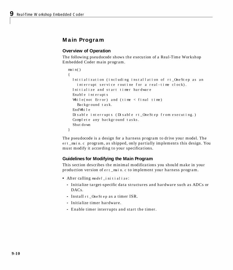
9 Real-Time Workshop Embedded Coder
9-10
Main Program
Overview of OperationThe following pseudocode shows the execution of a Real-Time WorkshopEmbedded Coder main program.
main(){Initialization (including installation of rt_OneStep as an interrupt service routine for a real-time clock).
Initialize and start timer hardwareEnable interuptsWhile(not Error) and (time < final time)Background task.
EndWhileDisable interrupts (Disable rt_OneStep from executing.)Complete any background tasks.Shutdown
}
The pseudocode is a design for a harness program to drive your model. Theert_main.c program, as shipped, only partially implements this design. Youmust modify it according to your specifications.
Guidelines for Modifying the Main ProgramThis section describes the minimal modifications you should make in yourproduction version of ert_main.c to implement your harness program.
• After calling model_initialize:
- Initialize target-specific data structures and hardware such as ADCs orDACs.
- Install rt_OneStep as a timer ISR.
- Initialize timer hardware.
- Enable timer interrupts and start the timer.
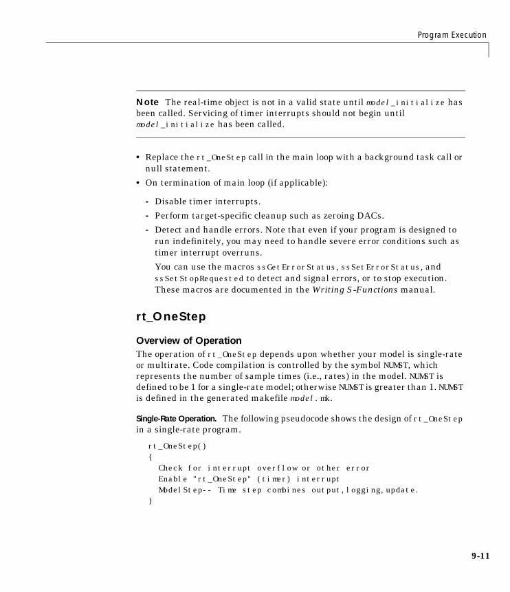
Program Execution
9-11
Note The real-time object is not in a valid state until model_initialize hasbeen called. Servicing of timer interrupts should not begin untilmodel_initialize has been called.
• Replace the rt_OneStep call in the main loop with a background task call ornull statement.
• On termination of main loop (if applicable):
- Disable timer interrupts.
- Perform target-specific cleanup such as zeroing DACs.
- Detect and handle errors. Note that even if your program is designed torun indefinitely, you may need to handle severe error conditions such astimer interrupt overruns.
You can use the macros ssGetErrorStatus, ssSetErrorStatus, andssSetStopRequested to detect and signal errors, or to stop execution.These macros are documented in the Writing S-Functions manual.
rt_OneStep
Overview of OperationThe operation of rt_OneStep depends upon whether your model is single-rateor multirate. Code compilation is controlled by the symbol NUMST, whichrepresents the number of sample times (i.e., rates) in the model. NUMST isdefined to be 1 for a single-rate model; otherwise NUMST is greater than 1. NUMSTis defined in the generated makefile model.mk.
Single-Rate Operation. The following pseudocode shows the design of rt_OneStepin a single-rate program.
rt_OneStep(){
Check for interrupt overflow or other errorEnable "rt_OneStep" (timer) interruptModelStep-- Time step combines output,logging,update.
}
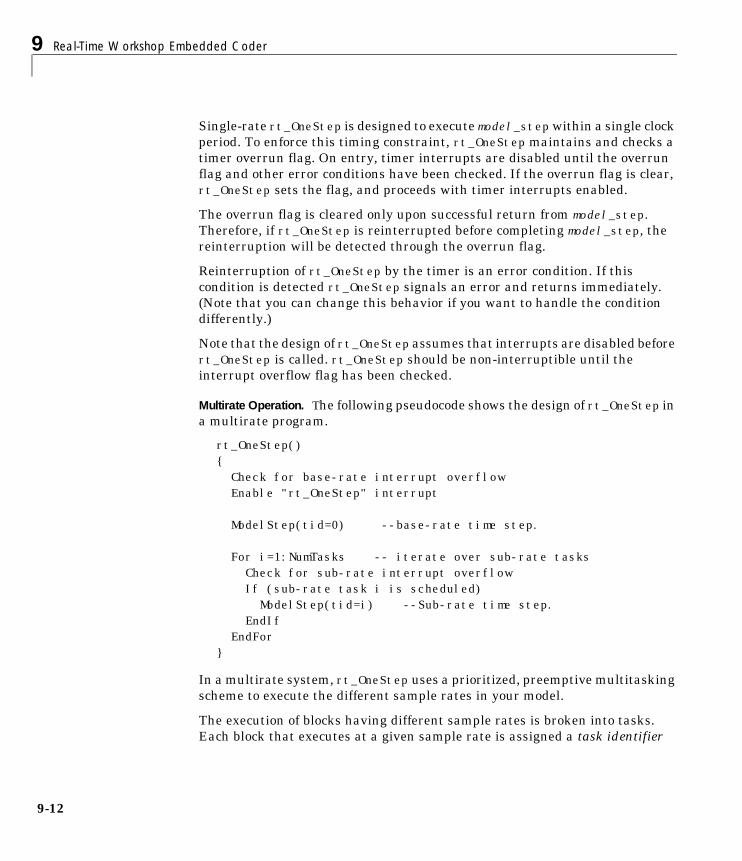
9 Real-Time Workshop Embedded Coder
9-12
Single-rate rt_OneStep is designed to execute model_stepwithin a single clockperiod. To enforce this timing constraint, rt_OneStep maintains and checks atimer overrun flag. On entry, timer interrupts are disabled until the overrunflag and other error conditions have been checked. If the overrun flag is clear,rt_OneStep sets the flag, and proceeds with timer interrupts enabled.
The overrun flag is cleared only upon successful return from model_step.Therefore, if rt_OneStep is reinterrupted before completing model_step, thereinterruption will be detected through the overrun flag.
Reinterruption of rt_OneStep by the timer is an error condition. If thiscondition is detected rt_OneStep signals an error and returns immediately.(Note that you can change this behavior if you want to handle the conditiondifferently.)
Note that the design of rt_OneStep assumes that interrupts are disabled beforert_OneStep is called. rt_OneStep should be non-interruptible until theinterrupt overflow flag has been checked.
Multirate Operation. The following pseudocode shows the design of rt_OneStep ina multirate program.
rt_OneStep(){Check for base-rate interrupt overflowEnable "rt_OneStep" interrupt
ModelStep(tid=0) --base-rate time step.
For i=1:NumTasks -- iterate over sub-rate tasksCheck for sub-rate interrupt overflowIf (sub-rate task i is scheduled)ModelStep(tid=i) --Sub-rate time step.
EndIfEndFor
}
In a multirate system, rt_OneStep uses a prioritized, preemptive multitaskingscheme to execute the different sample rates in your model.
The execution of blocks having different sample rates is broken into tasks.Each block that executes at a given sample rate is assigned a task identifier
Program Execution
9-13
(tid), which associates it with a task that executes at that rate. Where thereare NUMST tasks in the system, the range of task identifiers is 0..NUMST-1.
rt_OneStep prioritizes tasks, in descending order, by rate. The base-rate taskis the task that runs at the fastest rate in the system (the hardware clock rate).The base-rate task has highest priority (tid 0) . The next fastest task (tid 1)has the next highest priority, and so on down to the slowest, lowest prioritytask (tid NUMST-1).
The slower tasks, running at submultiples of the base rate, are called sub-ratetasks.
On each invocation, rt_OneStep makes one or more calls to model_step,passing in the appropriate tid. The tid informs model_step that all blockshaving that tid should execute. rt_OneStep always calls model_step (tid = 0)because the base-rate task must execute on every clock step.
On each clock tick, rt_OneStep also maintains scheduling counters and eventflags for each sub-rate task. Both the counters and the event flags areimplemented as arrays, indexed on tid.
The counters are, in effect, clock rate dividers that count up the sample periodassociated with each sub-rate task. The event flags indicate whether or not agiven task is scheduled for execution. When a counter indicates that a task’ssample period has elapsed, rt_OneStep sets the event flag for that task.
After updating its scheduling data structures and stepping the base-rate task,rt_OneStep iterates over the scheduling flags in tid order, callingmodel_step(tid) for any task whose flag is set. This ensures that tasks areexecuted in order of priority.
The event flag array and loop variables used by rt_OneStep are stored as local(stack) variables. This ensures that rt_OneStep is reentrant. If rt_OneStep isreinterrupted, higher priority tasks will preempt lower priority tasks. Uponreturn from interrupt, lower priority tasks will resume in the previouslyscheduled order.
Multirate rt_OneStep also maintains an array of timer overrun flags.rt_OneStep detects timer overrun, per task, by the same logic as single-ratert_OneStep.
Note that the design of rt_OneStep assumes that interrupts are disabled beforert_OneStep is called. rt_OneStep should be non-interruptible until thebase-rate interrupt overflow flag has been checked (see pseudo-code above).
9 Real-Time Workshop Embedded Coder
9-14
Guidelines for Modifying rt_OneSteprt_OneStep does not require extensive modification. The only requiredmodification is to re-enable interrupts after the overrun flag(s) and errorconditions have been checked. Comments in rt_OneStep indicate theappropriate place to add your code.
In multirate rt_OneStep, you can improve performance by unrolling for andwhile loops.
You may also want to replace the MODEL_STEP macro call(s) with model-specificcall(s). If so, see “How to Call the Entry Points Directly” on page 9-16.
In addition, you may choose to modify the overrun behavior to continueexecution after error recovery is complete.
You should not modify the way in which the counters are set in rt_OneStep.The rt_OneStep timing data structures (including the real-time object) andlogic are critical to correct operation of any Real-Time Workshop EmbeddedCoder program.
Model Entry Points
model_step
Calling Interface. The MODEL_STEP macro is the standard way to call your model’sgenerated step function.
In a single-rate model, the macro expands to a function call with the prototype
void model_step(void);
In a multirate model, the macro expands to a function call with the prototype
void model_step(int_T tid);
where tid is a task identifier. The tid is determined by logic withinrt_OneStep. (See “rt_OneStep” on page 9-11.)
Operation. model_step combines the model output and update functions into asingle routine. model_step is designed to be called at interrupt level fromrt_OneStep, which is assumed to be invoked as a timer ISR.
Program Execution
9-15
Single-Rate Operation. In a single-rate model, model_step computes the currentvalue of all blocks. If logging is enabled, model_step updates logging variables.If the model’s stop time is finite, model_step signals the end of execution whenthe current time equals the stop time.
Multirate Operation. In a multirate model, model_step execution is almostidentical to single-rate execution, except for the use of the task identifier (tid)argument.
The caller (rt_OneStep) assigns each block a tid. (See “rt_OneStep” on page9-11.) model_step uses the tid argument to determine which blocks have asample hit (and therefore should execute).
Note If the model’s stop time is set to inf, or if logging is disabled,model_step does not check the current time against the stop time. Therefore,the program runs indefinitely.
model_initialize
Calling Interface. The MODEL_INITIALIZE macro is the standard way to call yourmodel’s generated initialization code. The macro expands to a function callwith the prototype
void model_initialize(boolean_T firstTime);
Operation. If firstTime equals 1 (TRUE), model_initialize initializes thereal-time object and other data structures private to the model. If firstTimeequals 0 (FALSE), model_initialize resets the model’s states.
The generated code calls model_initialize once, passing in firstTime as1(TRUE).
model_terminate
Calling Interface. The MODEL_TERMINATE macro is a standard way to call yourmodel’s generated termination code. The macro expands to a function call withthe prototype
void model_terminate(void);

9 Real-Time Workshop Embedded Coder
9-16
Operation. When model_terminate is called, blocks that have a terminatefunction execute their terminate code. If logging is enabled, model_terminateends data logging. model_terminate should only be called once. If yourapplication runs indefinitely, you do not need the model_terminate function.
If you do not require a terminate function, see “Basic Code Generation Options”on page 9–20 for information on using the Terminate function requiredoption.
How to Call the Entry Points DirectlyYou can replace the generated macro calls with direct calls to the entry points.This is necessary when interfacing your code with code generated from morethan one model. In such cases, the macro calls are ambiguous. Includemodel_export.h to make the entry points visible to your code, as in thefollowing code fragment.
#include "modelA_Export.h" /* Make model A entry points visible */#include "modelB_Export.h" /* Make model B entry points visible */
void myHandWrittenFunction(void){const char_T *errStatus;
modelA_initialize(1); /* Call model A initializer */modelB_initialize(1); /* Call model B initializer *//* Refer to model A’s real-time Object */errStatus = ssGetErrorStatus(modelA_rtO);/* Refer to model B’s real-time Object */errStatus = ssGetErrorStatus(modelB_rtO);
}
Note If you are modifying model_step calls in multirate rt_OneStep, takecare to pass in the correct tid argument. The first call, which steps the modelfor the base sample time, always passes in tid 0. The calls made in thesub-rate loop always pass in the loop variable i.
Automatic S-Function Wrapper Generation
9-17
Automatic S-Function Wrapper GenerationAn S-function wrapper is an S-function that calls your C code from withinSimulink. S-function wrappers provide a standard interface between Simulinkand externally written code, allowing you to integrate your code into a modelwith minimal modification. For a complete description of wrapper S-functions,see the Writing S-Functions manual.
Using the Real-Time Workshop Embedded Coder Create Simulink(S-Function) block option, you can build, in one automated step:
• A noninlined C MEX S-function wrapper that calls Real-Time WorkshopEmbedded Coder generated code.
• A model containing the generated S-function block, ready for use with otherblocks or models.
This is useful for code validation and simulation acceleration purposes.
When Create Simulink (S-Function) block option is on, the Real-TimeWorkshop generates an additional source code file, model_sf.c, in the builddirectory. This module contains the S-function that calls the Real-TimeWorkshop Embedded Coder code that you deploy. This S-function can be usedwithin Simulink.
The build process then compiles and links model_sf.c with model.c and theother Real-Time Workshop Embedded Coder generated code modules, buildinga MEX-file.The MEX-file is named model_sf.mexext. (mexext is the fileextension for MEX-files on your platform, as given by the MATLAB mexextcommand.) The MEX-file is stored in your working directory. Finally, theReal-Time Workshop creates and opens an untitled model containing thegenerated S-Function block.
LimitationsIt is not possible to create multiple instances of a Real-Time WorkshopEmbedded Coder generated S-Function block within a model, because the codeuses static memory allocation.
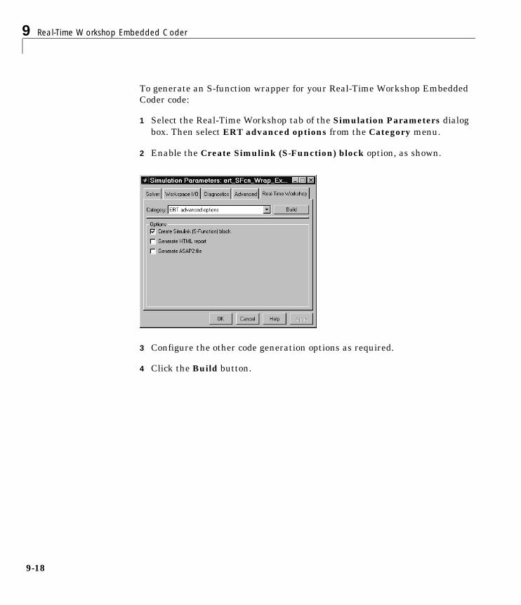
9 Real-Time Workshop Embedded Coder
9-18
To generate an S-function wrapper for your Real-Time Workshop EmbeddedCoder code:
1 Select the Real-Time Workshop tab of the Simulation Parameters dialogbox. Then select ERT advanced options from the Category menu.
2 Enable the Create Simulink (S-Function) block option, as shown.
3 Configure the other code generation options as required.
4 Click the Build button.
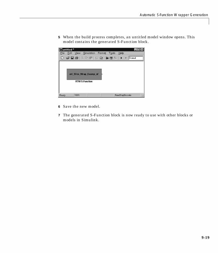
Automatic S-Function Wrapper Generation
9-19
5 When the build process completes, an untitled model window opens. Thismodel contains the generated S-Function block.
6 Save the new model.
7 The generated S-Function block is now ready to use with other blocks ormodels in Simulink.
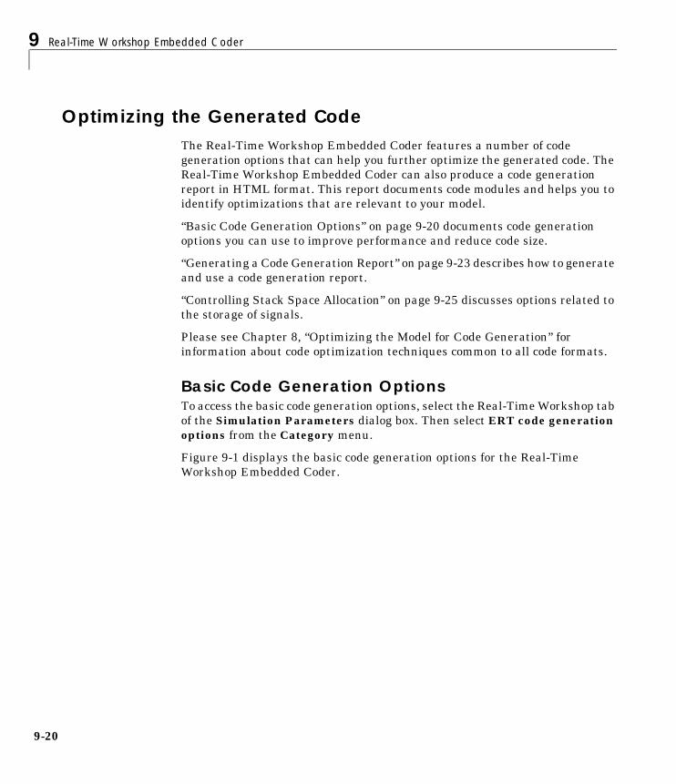
9 Real-Time Workshop Embedded Coder
9-20
Optimizing the Generated CodeThe Real-Time Workshop Embedded Coder features a number of codegeneration options that can help you further optimize the generated code. TheReal-Time Workshop Embedded Coder can also produce a code generationreport in HTML format. This report documents code modules and helps you toidentify optimizations that are relevant to your model.
“Basic Code Generation Options” on page 9-20 documents code generationoptions you can use to improve performance and reduce code size.
“Generating a Code Generation Report” on page 9-23 describes how to generateand use a code generation report.
“Controlling Stack Space Allocation” on page 9-25 discusses options related tothe storage of signals.
Please see Chapter 8, “Optimizing the Model for Code Generation” forinformation about code optimization techniques common to all code formats.
Basic Code Generation OptionsTo access the basic code generation options, select the Real-Time Workshop tabof the Simulation Parameters dialog box. Then select ERT code generationoptions from the Category menu.
Figure 9-1 displays the basic code generation options for the Real-TimeWorkshop Embedded Coder.
Optimizing the Generated Code
9-21
Figure 9-1: Basic Code Generation Options
Note ert_main.c contains certain compile-time error checks on codegeneration options, intended for use during simulation only. You shouldremove these error checks, as instructed below, from your production versionof ert_main.c
Setting the code generation options as follows will result in more highlyoptimized code:
• Deselect the MAT-file logging check box.
Also, remove or comment out the #if MAT_FILE... error check in yourproduction version of ert_main.c.
Note that disabling logging causes the program to run indefinitely,regardless of the setting of the model’s stop time.
• Deselect the Initialize internal data and Initialize external I/O data checkboxes.
Initializing the internal and external data is a precaution and may not benecessary for your application. Many embedded application environments
9 Real-Time Workshop Embedded Coder
9-22
initialize all RAM to zero at startup. Therefore, reinitializing RAM to zero isredundant.
Note that nonzero initialization of your program’s data structures is stillperformed when Initialize internal data and Initialize external I/O dataare selected.
• Deselect the Terminate function required check box if you do not require aterminate function for your model.
Also, remove or comment out the following in your production version ofert_main.c:
- The #if TERMFCN... error check
- The call to MODEL_TERMINATE
• Select the Single output/update function check box. Combining the outputand update functions is the default. This option generates the model_stepcall, which reduces overhead and allows the Real-Time Workshop to usemore local variables in the step function of the model.
If you do not want to combine output and update functions, make thefollowing changes in your production version of ert_main.c:
- Replace calls to MODEL_STEP with calls to model_output andmodel_update.
- Remove the #if ONESTEPFCN... error check.
• If your application uses only integer arithmetic, select the Integer code onlyoption to ensure that generated code contains no floating-point data oroperations. When this option is selected, an error is raised if any nonintegerdata or expressions are encountered during code generation. The errormessage reports the offending blocks and parameters.
Generating Code from SubsystemsNote that when generating code from a subsystem, it is recommended that youset the sample times of all subsystem inports explicitly.
Generating Block CommentsWhen the Insert block descriptions in code option is selected, comments areinserted into the code generated for any blocks that have text in theirDescription fields.
Optimizing the Generated Code
9-23
To generate block comments:
1 Right-click on the block you want to comment. Select Block Properties fromthe context menu. The Block Properties dialog box opens.
2 Type the comment into the Description field.
3 Select the Insert block descriptions in code option in the ERT codegeneration options category of the Real-Time Workshop page.
Note For virtual blocks or blocks that have been removed due to blockreduction optimizations, no comments are generated.
Generating a Code Generation ReportThe Real-Time Workshop Embedded Coder code generation report is an HTMLfile consisting of several sections:
• The Summary section lists version and date information, TLC options usedin code generation, and Simulink model settings.
• The Optimizations section lists the optimizations used during the build, andalso those that are available. If options were chosen that generatednon-optimal code, they are marked in red. This section can help you selectoptions that will better optimize your code.
• The Generated Source Files section contains a table of source code filesgenerated from subsystems (if any) in your model. Each row contains ahyperlink to the relevant subsystem. You can click on the hyperlink to viewthe subsystem in a Simulink model window.
To generate a code generation report:
1 Select the Real-Time Workshop tab of the Simulation Parameters dialogbox. Then select Advanced code generation options from the Categorymenu.
2 Select Generate HTML report, as shown in this picture.
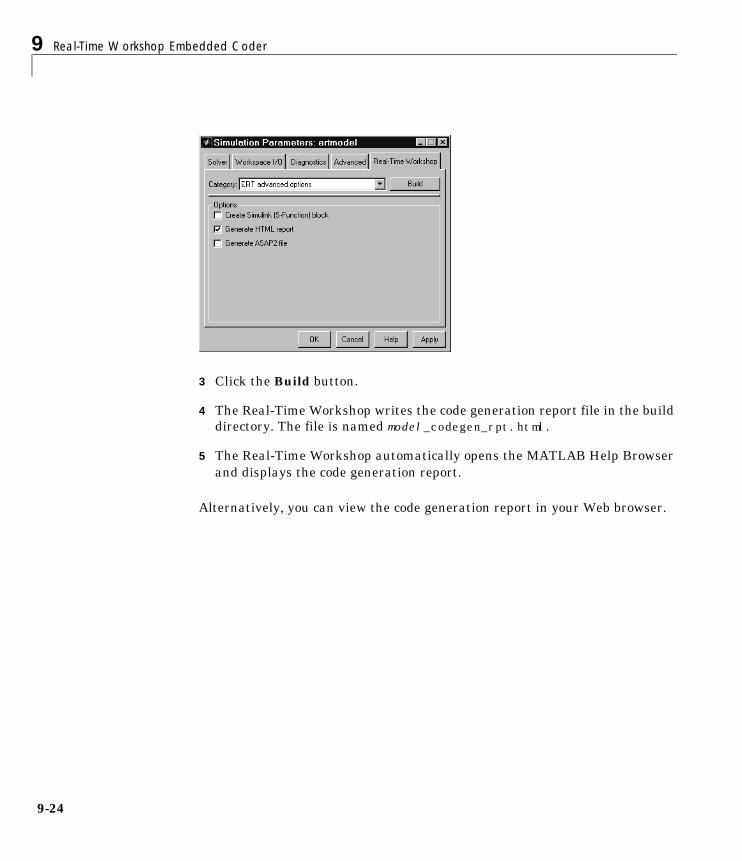
9 Real-Time Workshop Embedded Coder
9-24
3 Click the Build button.
4 The Real-Time Workshop writes the code generation report file in the builddirectory. The file is named model_codegen_rpt.html.
5 The Real-Time Workshop automatically opens the MATLAB Help Browserand displays the code generation report.
Alternatively, you can view the code generation report in your Web browser.
Optimizing the Generated Code
9-25
Controlling Stack Space AllocationThe Real-Time Workshop offers a number of options that let you control howsignals in your model are stored and represented in the generated code. Thissection discusses options that:
• Let you control whether signal storage is declared in global memory space,or locally in functions (i.e., in stack variables).
• Control the allocation of stack space when using local storage.
For a complete discussion of signal storage options, see “Signals: Storage,Optimization, and Interfacing” on page 3-65.
If you want to store signals in stack space, you must turn the Local blockoutputs option on. To do this:
1 Select the Advanced tab of the Simulation Parameters dialog box. Makesure that the Signal storage reuse is on. If Signal storage reuse is off, theLocal block outputs option is not available.
2 Click Apply if necessary.
3 Select the Real-Time Workshop tab of the Simulation Parameters dialogbox.
4 From the Category menu, select General code generation options.
5 Check the Local block outputs option. Click Apply if necessary.
Your embedded application may be constrained by limited stack space. Whenthe Local block outputs option is on, you can limit the use of stack space byusing the following Target Language Compiler variables:
• MaxStackSize: the total allocation size of local variables that are declared byall functions in the entire model may not exceed MaxStackSize (in bytes).MaxStackSize can be any positive integer. If the total size of local variablesexceeds this maximum, the Target Language Compiler will allocate theremaining variables in global, rather than local, memory.
• MaxStackVariableSize: limits the size of any local variable declared in afunction to N bytes, where N>0. A variable whose size exceeds

9 Real-Time Workshop Embedded Coder
9-26
MaxStackVariableSize will be allocated in global, rather than local,memory.
To set either of these variables, use assign statements in the system target file(ert.tlc), as in the following example.
%assign MaxStackSize = 4096
It is recommended that you write your %assign statements in the Configure RTW code generation settings section of the system target file. The %assignstatement is described in the Target Language Compiler Reference Guide.

Advanced Code Generation Options
9-27
Advanced Code Generation OptionsTo access the advanced Real-Time Workshop Embedded Coder code generationoptions, select the Real-Time Workshop tab of the Simulation Parametersdialog box. Then select Advanced code generation options from theCategory menu.
Figure 9-2 displays the advanced code generation options for the Real-TimeWorkshop Embedded Coder.
Figure 9-2: Advanced Code Generation Options
Create Simulink (S-Function) BlockSee “Automatic S-Function Wrapper Generation” on page 9-17 for informationon this feature.
Generate HTML ReportSee “Generating a Code Generation Report” on page 9-23 for information onthis feature.

9 Real-Time Workshop Embedded Coder
9-28
Generate ASAP2 FileThe Real-Time Workshop Embedded Coder Generate ASAP2 File codegeneration option lets you export an ASAP2 file containing information aboutyour model during the code generation process.
The ASAP2 file generation process requires information about your model'sparameters and signals. Some of this information is contained in the modelitself. The rest must be supplied by using Simulink data objects with thenecessary properties. Simulink provides two data classes to assist you inproviding the necessary information. See “Generating ASAP2 Files” in theReal-Time Workshop online documentation for information on this feature.
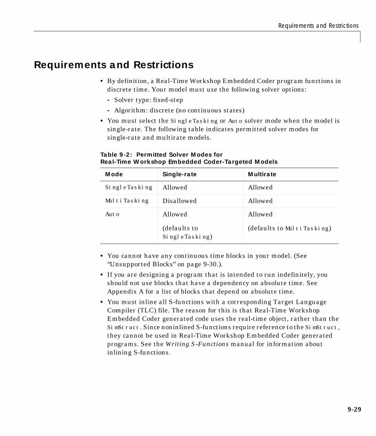
Requirements and Restrictions
9-29
Requirements and Restrictions• By definition, a Real-Time Workshop Embedded Coder program functions in
discrete time. Your model must use the following solver options:
- Solver type: fixed-step
- Algorithm: discrete (no continuous states)
• You must select the SingleTasking or Auto solver mode when the model issingle-rate. The following table indicates permitted solver modes forsingle-rate and multirate models.
• You cannot have any continuous time blocks in your model. (See“Unsupported Blocks” on page 9-30.).
• If you are designing a program that is intended to run indefinitely, youshould not use blocks that have a dependency on absolute time. SeeAppendix A for a list of blocks that depend on absolute time.
• You must inline all S-functions with a corresponding Target LanguageCompiler (TLC) file. The reason for this is that Real-Time WorkshopEmbedded Coder generated code uses the real-time object, rather than theSimStruct. Since noninlined S-functions require reference to the SimStruct,they cannot be used in Real-Time Workshop Embedded Coder generatedprograms. See the Writing S-Functions manual for information aboutinlining S-functions.
Table 9-2: Permitted Solver Modes forReal-Time Workshop Embedded Coder-Targeted Models
Mode Single-rate Multirate
SingleTasking Allowed Allowed
MultiTasking Disallowed Allowed
Auto Allowed
(defaults toSingleTasking)
Allowed
(defaults to MultiTasking)
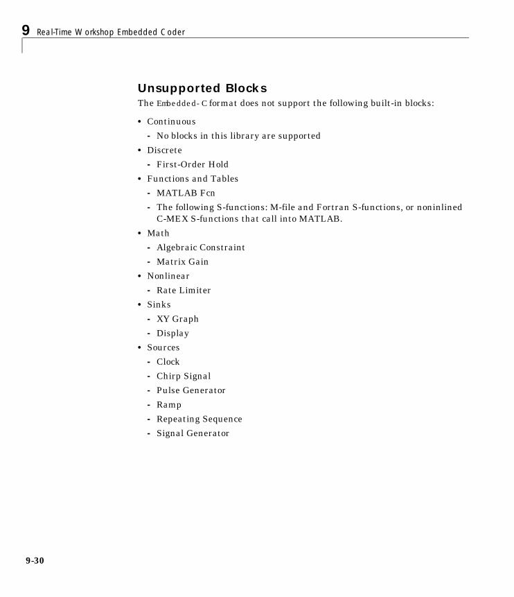
9 Real-Time Workshop Embedded Coder
9-30
Unsupported BlocksThe Embedded-C format does not support the following built-in blocks:
• Continuous
- No blocks in this library are supported
• Discrete
- First-Order Hold
• Functions and Tables
- MATLAB Fcn
- The following S-functions: M-file and Fortran S-functions, or noninlinedC-MEX S-functions that call into MATLAB.
• Math
- Algebraic Constraint
- Matrix Gain
• Nonlinear
- Rate Limiter
• Sinks
- XY Graph
- Display
• Sources
- Clock
- Chirp Signal
- Pulse Generator
- Ramp
- Repeating Sequence
- Signal Generator

System Target File and Template Makefiles
9-31
System Target File and Template MakefilesThe Real-Time Workshop Embedded Coder system target file is ert.tlc.
The Real-Time Workshop provides template makefiles for the Real-TimeWorkshop Embedded Coder in the following development environments:
• ert_bc.tmf — Borland C
• ert_lcc.tmf — LCC compiler
• ert_unix.tmf — UNIX host
• ert_vc.tmf — Visual C
• ert_watc.tmf — Watcom C

9 Real-Time Workshop Embedded Coder
9-32
10
The S-Function Target
Introduction . . . . . . . . . . . . . . . . . . . . 10-2Intellectual Property Protection . . . . . . . . . . . . . 10-3
Creating an S-Function Block from a Subsystem . . . . 10-4
Tunable Parameters in Generated S-Functions . . . . 10-10
Automated S-Function Generation . . . . . . . . . 10-12
Restrictions . . . . . . . . . . . . . . . . . . . 10-15
Unsupported Blocks . . . . . . . . . . . . . . . . 10-16
System Target File and Template Makefiles . . . . . . 10-17System Target File . . . . . . . . . . . . . . . . . 10-17Template Makefiles . . . . . . . . . . . . . . . . . 10-17
10 The S-Function Target
10-2
IntroductionUsing the S-function target, you can build an S-function component and use itas an S-Function block in another model. The S-function code format used bythe S-function target generates code that conforms to the Simulink C MEXS-function application programming interface (API). Applications of thisformat include:
• Conversion of a model to a component. You can generate an S-Function blockfor a model, m1. Then, you can place the generated S-Function block inanother model, m2. Regenerating code for m2 does not require regeneratingcode for m1.
• Conversion of a subsystem to a component. By extracting a subsystem to aseparate model, and generating an S-Function block from that model, youcan create a reusable component from the subsystem. See “Creating anS-Function Block from a Subsystem” on page 10-4 for an example of thisprocedure.
• Speeding up simulation. In many cases, an S-function generated from amodel performs more efficiently than the original model.
• Code reuse. You can incorporate multiple instances of one model insideanother without replicating the code for each instance. Each instance willcontinue to maintain its own unique data.
The S-function target generates noninlined S-functions. You can generate anexecutable from a model that contains generated S-functions by using thegeneric real-time or real-time malloc targets. You cannot use the Real-TimeWorkshop Embedded Coder target for this purpose, since it requires inlinedS-functions.
You can place a generated S-Function block into another model from which youcan generate another S-function format. This allows any level of nestedS-functions.
Note that sample times propagation for the S-function code format is slightlydifferent from the other code formats. A generated S-Function block willinherit its sample time from the model in which it is placed if no blocks in theoriginal model specify their sample times.
Introduction
10-3
Intellectual Property ProtectionIn addition to the technical applications of the S-function target listed above,you can use the S-function target to protect your designs and algorithms. Bygenerating an S-function from a proprietary model or algorithm, you can sharethe model’s functionality without providing the source code. You need onlyprovide the binary .dll or MEX-file object to users.
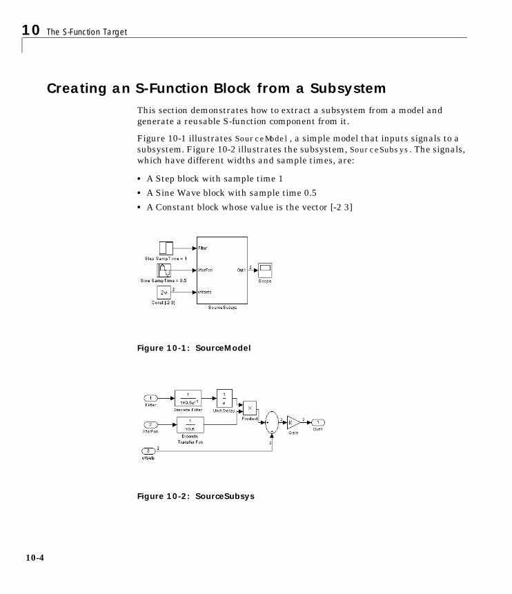
10 The S-Function Target
10-4
Creating an S-Function Block from a SubsystemThis section demonstrates how to extract a subsystem from a model andgenerate a reusable S-function component from it.
Figure 10-1 illustrates SourceModel, a simple model that inputs signals to asubsystem. Figure 10-2 illustrates the subsystem, SourceSubsys. The signals,which have different widths and sample times, are:
• A Step block with sample time 1
• A Sine Wave block with sample time 0.5
• A Constant block whose value is the vector [-2 3]
Figure 10-1: SourceModel
Figure 10-2: SourceSubsys
Creating an S-Function Block from a Subsystem
10-5
Our objective is to extract SourceSubsys from the model and build anS-Function block from it, using the S-function target. We want the S-Functionblock to perform identically to the subsystem from which it was generated.
Note that in this model, SourceSubsys inherits sample times and signal widthsfrom its input signals. If an S-Function block is built from SourceSubsys,without explicitly setting input widths and sample times, the new block willinherit its sample times and signal widths from the model in which it is placed.
In this example, however, we want the S-Function block to retain theproperties of SourceSubsys as it exists in SourceModel. Before building thesubsystem as a separate S-function component, the inport sample times andwidths must be set explicitly. In addition, the solver parameters of theS-function component must be the same as those of the original model. Thisensures that the generated S-function component will operate identically to theoriginal subsystem.
To build SourceSubsys as an S-function component:
1 Create a new model and copy/paste SourceSubsys into the empty window.
2 Set the signal widths and sample times of inports inside SourceSubsys suchthat they match those of the signals in the original model. Inport 1, Filter,has a width of 1 and a a sample time of 1. Inport 2, Xferfcn, has a width of1 and a sample time of 0.5. Inport 3, offsets, has a width of 2 and aninherited sample time of 1.
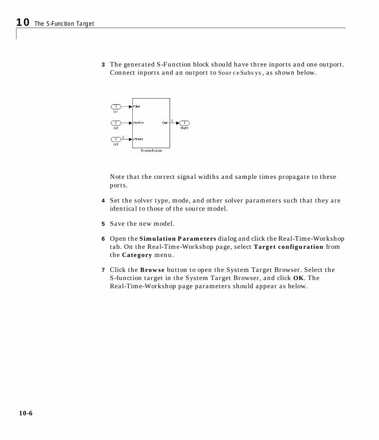
10 The S-Function Target
10-6
3 The generated S-Function block should have three inports and one outport.Connect inports and an outport to SourceSubsys, as shown below.
Note that the correct signal widths and sample times propagate to theseports.
4 Set the solver type, mode, and other solver parameters such that they areidentical to those of the source model.
5 Save the new model.
6 Open the Simulation Parameters dialog and click the Real-Time-Workshoptab. On the Real-Time-Workshop page, select Target configuration fromthe Category menu.
7 Click the Browse button to open the System Target Browser. Select theS-function target in the System Target Browser, and click OK. TheReal-Time-Workshop page parameters should appear as below.
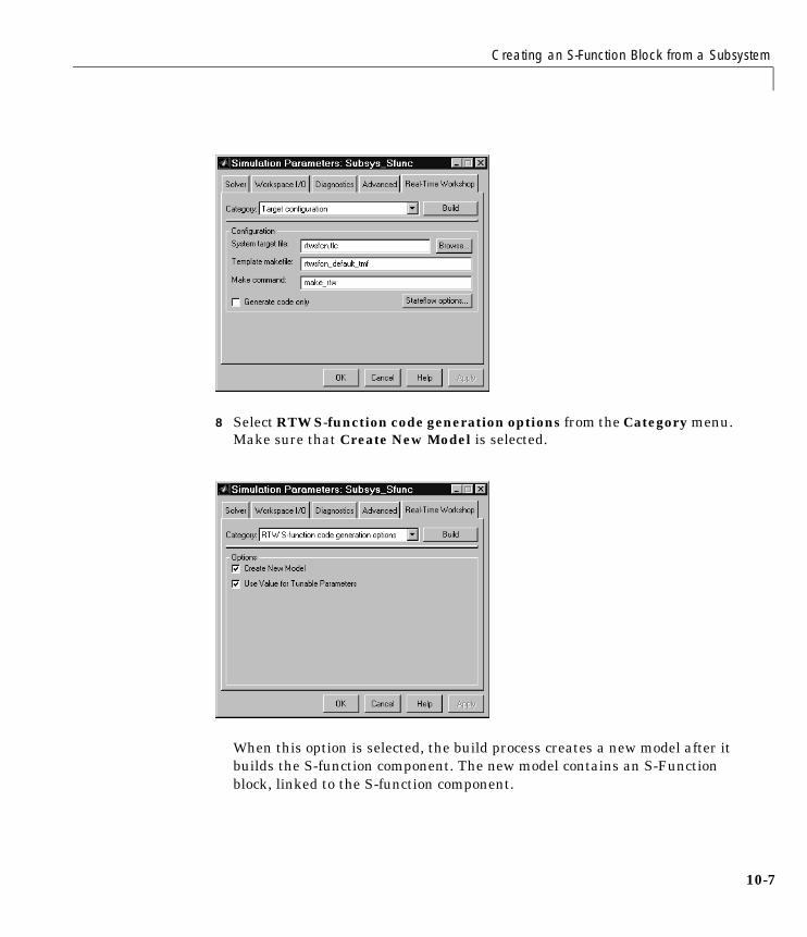
Creating an S-Function Block from a Subsystem
10-7
8 Select RTW S-function code generation options from the Category menu.Make sure that Create New Model is selected.
When this option is selected, the build process creates a new model after itbuilds the S-function component. The new model contains an S-Functionblock, linked to the S-function component.
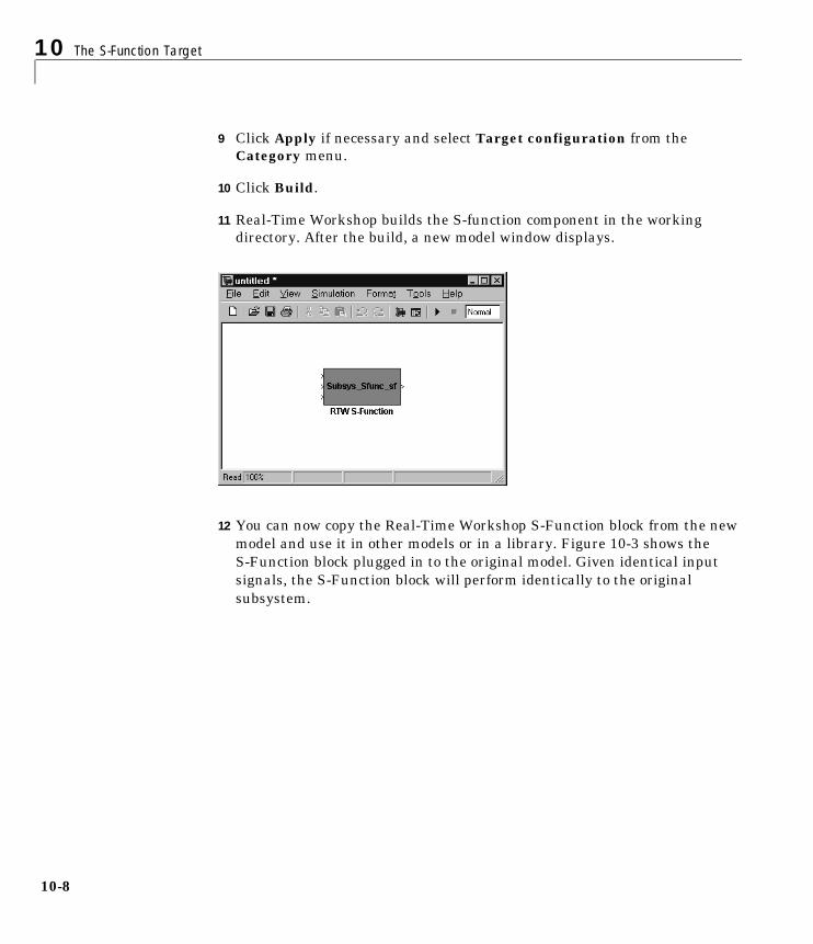
10 The S-Function Target
10-8
9 Click Apply if necessary and select Target configuration from theCategory menu.
10 Click Build.
11 Real-Time Workshop builds the S-function component in the workingdirectory. After the build, a new model window displays.
12 You can now copy the Real-Time Workshop S-Function block from the newmodel and use it in other models or in a library. Figure 10-3 shows theS-Function block plugged in to the original model. Given identical inputsignals, the S-Function block will perform identically to the originalsubsystem.

Creating an S-Function Block from a Subsystem
10-9
Figure 10-3: Generated S-Function Plugged into SourceModel
Note that the speed at which the S-Function block executes is typically fasterthan the original model. This difference in speed is more pronounced for largerand more complicated models. By using generated S-functions, you canincrease the efficiency of your modeling process.
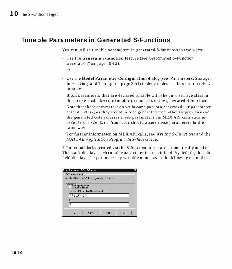
10 The S-Function Target
10-10
Tunable Parameters in Generated S-FunctionsYou can utilize tunable parameters in generated S-functions in two ways:
• Use the Generate S-function feature (see “Automated S-FunctionGeneration” on page 10-12).
or
• Use the Model Parameter Configuration dialog (see “Parameters: Storage,Interfacing, and Tuning” on page 3-51) to declare desired block parameterstunable.
Block parameters that are declared tunable with the auto storage class inthe source model become tunable parameters of the generated S-function.
Note that these parameters do not become part of a generated rtP parameterdata structure, as they would in code generated from other targets. Instead,the generated code accesses these parameters via MEX API calls such asmxGetPr or mxGetData. Your code should access these parameters in thesame way.
For further information on MEX API calls, see Writing S-Functions and theMATLAB Application Program Interface Guide.
S-Function blocks created via the S-function target are automatically masked.The mask displays each tunable parameter in an edit field. By default, the editfield displays the parameter by variable name, as in the following example.
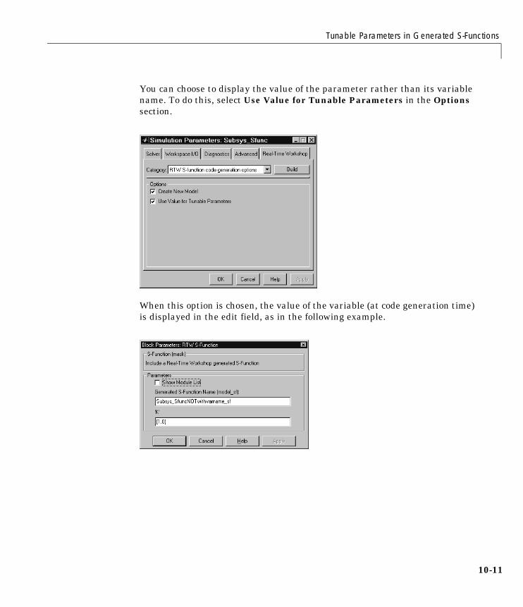
Tunable Parameters in Generated S-Functions
10-11
You can choose to display the value of the parameter rather than its variablename. To do this, select Use Value for Tunable Parameters in the Optionssection.
When this option is chosen, the value of the variable (at code generation time)is displayed in the edit field, as in the following example.
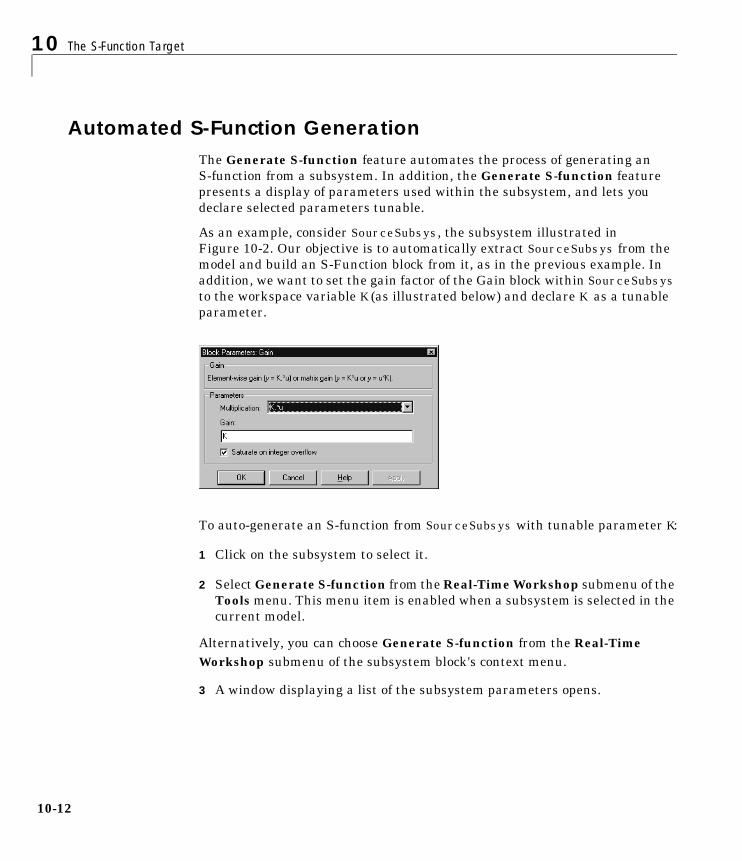
10 The S-Function Target
10-12
Automated S-Function GenerationThe Generate S-function feature automates the process of generating anS-function from a subsystem. In addition, the Generate S-function featurepresents a display of parameters used within the subsystem, and lets youdeclare selected parameters tunable.
As an example, consider SourceSubsys, the subsystem illustrated inFigure 10-2. Our objective is to automatically extract SourceSubsys from themodel and build an S-Function block from it, as in the previous example. Inaddition, we want to set the gain factor of the Gain block within SourceSubsysto the workspace variable K (as illustrated below) and declare K as a tunableparameter.
To auto-generate an S-function from SourceSubsys with tunable parameter K:
1 Click on the subsystem to select it.
2 Select Generate S-function from the Real-Time Workshop submenu of theTools menu. This menu item is enabled when a subsystem is selected in thecurrent model.
Alternatively, you can choose Generate S-function from the Real-TimeWorkshop submenu of the subsystem block's context menu.
3 A window displaying a list of the subsystem parameters opens.
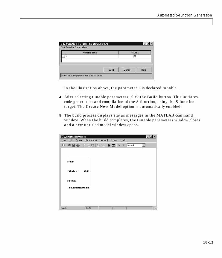
Automated S-Function Generation
10-13
In the illustration above, the parameter K is declared tunable.
4 After selecting tunable parameters, click the Build button. This initiatescode generation and compilation of the S-function, using the S-functiontarget. The Create New Model option is automatically enabled.
5 The build process displays status messages in the MATLAB commandwindow. When the build completes, the tunable parameters window closes,and a new untitled model window opens.
10 The S-Function Target
10-14
6 The model window contains an S-Function block, subsys_blk, where subsysis the name of the subsystem from which the block was generated.
The generated S-function component, subsys, is stored in the workingdirectory. The generated source code for the S-function is written to a builddirectory, subsys_sfcn_rtw.
7 Note that the untitled generated model does not persist, unless you save itvia the File menu.
8 Note that the generated S-Function block has inports and outports whosewidths and sample times correspond to those of the original model.
The following code fragment, from the mdlOutputs routine of the generatedS-function code (in SourceSubsys_sf.c), illustrates how the tunable variable Kis referenced via calls to the MEX API.
static void mdlOutputs(SimStruct *S, int_T tid)...real_T rtb_temp3[2];.../* Gain Block: <S1>/Gain */rtb_temp3[0] *= ((*(real_T *)(mxGetData(K(S)))));rtb_temp3[1] *= ((*(real_T *)(mxGetData(K(S)))));
Note In automatic S-function generation, the Use Value for TunableParameters option is always set to its default value (off).
Restrictions
10-15
Restrictions• Hand-written S-functions without corresponding TLC files must contain
exception-free code. For more information on exception-free code, refer to“Exception-Free Code” in Writing S-Functions.
• If you modify the source model that generated an S-Function block, theReal-Time Workshop does not automatically rebuild models containing thegenerated S-Function block.
10 The S-Function Target
10-16
Unsupported BlocksThe S-function format does not support the following built-in blocks:
• MATLAB Fcn Block
• S-Function blocks containing any of the following:
- M-file S-functions
- Fortran S-functions
- C MEX S-functions that call into MATLAB
• Scope block
• To Workspace block
System Target File and Template Makefiles
10-17
System Target File and Template MakefilesThe following system target file and template makefiles are provided for usewith the S-function target.
System Target File• rtwsfcn.tlc
Template Makefiles• rtwsfcn_bc.tmf — Borland C
• rtwsfcn_lcc.tmf — LCC compiler
• rtwsfc_unix.tmf — UNIX host
• rtwsfcn_vc.tmf — Visual C
• rtwsfcn_watc.tmf — Watcom C

10 The S-Function Target
10-18

11Real-Time WorkshopRapid Simulation Target
Introduction . . . . . . . . . . . . . . . . . . . . 11-2
Building for the Rapid Simulation Target . . . . . . . 11-4Running a Rapid Simulation . . . . . . . . . . . . . . 11-5Simulation Performance . . . . . . . . . . . . . . . 11-12Batch and Monte Carlo Simulations . . . . . . . . . . 11-12
11 Real-Time Workshop Rapid Simulation Target
11-2
IntroductionThe Real-Time Workshop rapid simulation target (rsim) consists of a set oftarget files for nonreal-time execution on your host computer. You can use rsimto generate fast, stand-alone simulations that allow batch parameter tuningand loading of new simulation data (signals) from a standard MATLABMAT-file without needing to recompile your model.
C code generated from Real-Time Workshop is highly optimized to provide fastexecution of discrete-time systems or systems that use a fixed-step solver. Thespeed of the generated code also makes it ideal for batch or Monte Carlosimulation. The run-time interface for the rapid simulation target enables thegenerated code to read and write data to standard MATLAB MAT-files. Usingthese support files, rsim reads new signals and parameters from MAT-files atthe start of the simulation.
After building an rsim executable with Real-Time Workshop and anappropriate C compiler for your host computer, you can perform anycombination of the following by using command line options. Withoutrecompiling, the rapid simulation target allows you to:
• Specify a new file(s) that provides input signals for From File blocks
• Specify a new file that provides input signals with any Simulink data type(double, float, int32, uint32, int16, uint16, int8, uint8, and complex datatypes) by using the From Workspace block
• Replace the entire block diagram parameter vector and run a simulation
• Specify a new stop time for ending the stand-alone simulation
• Specify a new name of the MAT-file used to save model output data
• Specify name(s) of the MAT-files used to save data connected to To Fileblocks
You can run these options:
• Directly from your operating system command line (for example, DOS box orUNIX shell) or
• By using the bang (!) command with a command string at the MATLABprompt
Therefore, you can easily write simple scripts that will run a set of simulationsin sequence while using new data sets. These scripts can be written to provide

11-3
unique filenames for both input parameters and input signals, as well asoutput filenames for the entire model or for To File blocks.
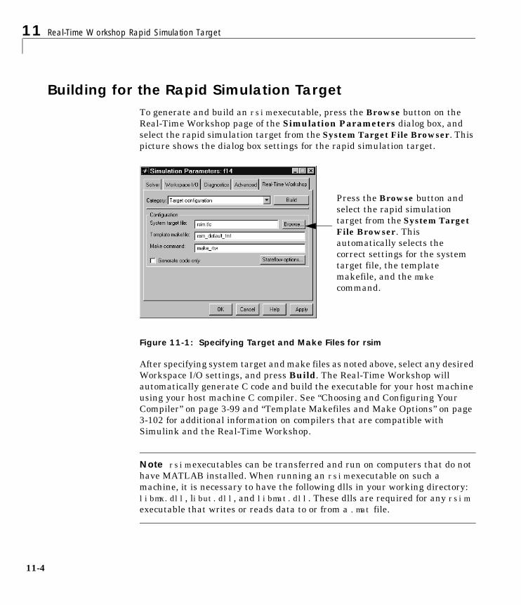
11 Real-Time Workshop Rapid Simulation Target
11-4
Building for the Rapid Simulation TargetTo generate and build an rsim executable, press the Browse button on theReal-Time Workshop page of the Simulation Parameters dialog box, andselect the rapid simulation target from the System Target File Browser. Thispicture shows the dialog box settings for the rapid simulation target.
Figure 11-1: Specifying Target and Make Files for rsim
After specifying system target and make files as noted above, select any desiredWorkspace I/O settings, and press Build. The Real-Time Workshop willautomatically generate C code and build the executable for your host machineusing your host machine C compiler. See “Choosing and Configuring YourCompiler” on page 3-99 and “Template Makefiles and Make Options” on page3-102 for additional information on compilers that are compatible withSimulink and the Real-Time Workshop.
Note rsim executables can be transferred and run on computers that do nothave MATLAB installed. When running an rsim executable on such amachine, it is necessary to have the following dlls in your working directory:libmx.dll, libut.dll, and libmat.dll. These dlls are required for any rsimexecutable that writes or reads data to or from a .mat file.
Press the Browse button andselect the rapid simulationtarget from the System TargetFile Browser. Thisautomatically selects thecorrect settings for the systemtarget file, the templatemakefile, and the makecommand.

Building for the Rapid Simulation Target
11-5
Running a Rapid SimulationThe rapid simulation target lets you run a simulation similar to the genericreal-time (GRT) target provided by the Real-Time Workshop. This simulationdoes not use timer interrupts, and therefore is a nonreal-time simulationenvironment. The difference between GRT and rsim simulations is that rsimallows you to change parameter values or input signals at the start of asimulation without the need to generate code or recompile. The GRT target, onthe other hand, is a starting point for targeting a new processor.
A single build of your model can be used to study effects from varyingparameters or input signals. Command line arguments provide the necessarymechanism to specify new data for your simulation. This table lists allavailable command line options.
Specifying a New Signal Data File for a From File BlockTo understand how to specify new signal data for a From File block, create aworking directory and connect to that directory. Open the model rsimtfdemoby typing
Table 11-1: rsim Command Line Options
Command Line Option Description
model -f old.mat=new.mat Read From File block input signal data froma replacement MAT-file.
model -o newlogfile.mat Write MAT-file logging data to a file namednewlogfile.mat.
model -p filename.mat Read a new (replacement) parameter vectorfrom a file named filename.mat.
model -s <stoptime> Run the simulation until the time value<stoptime> is reached.
model -t old.mat=new.mat The original model specified saving signalsto the output file old.mat. For this run usethe file new.mat for saving signal data.
model -v Run in verbose mode.
model -h Display a help message listing options.
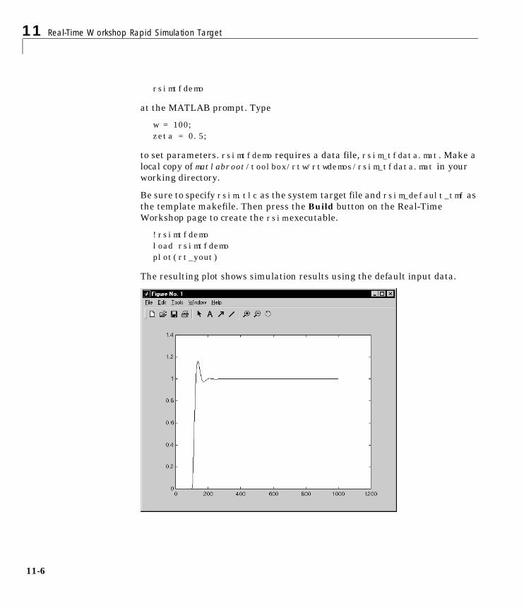
11 Real-Time Workshop Rapid Simulation Target
11-6
rsimtfdemo
at the MATLAB prompt. Type
w = 100;zeta = 0.5;
to set parameters. rsimtfdemo requires a data file, rsim_tfdata.mat. Make alocal copy of matlabroot/toolbox/rtw/rtwdemos/rsim_tfdata.mat in yourworking directory.
Be sure to specify rsim.tlc as the system target file and rsim_default_tmf asthe template makefile. Then press the Build button on the Real-TimeWorkshop page to create the rsim executable.
!rsimtfdemoload rsimtfdemoplot(rt_yout)
The resulting plot shows simulation results using the default input data.
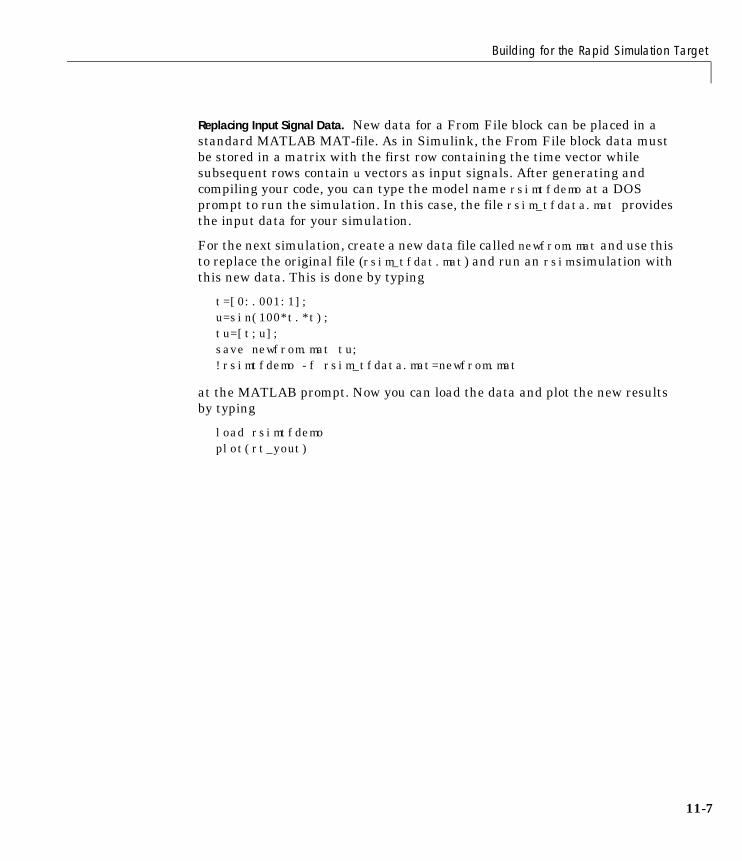
Building for the Rapid Simulation Target
11-7
Replacing Input Signal Data. New data for a From File block can be placed in astandard MATLAB MAT-file. As in Simulink, the From File block data mustbe stored in a matrix with the first row containing the time vector whilesubsequent rows contain u vectors as input signals. After generating andcompiling your code, you can type the model name rsimtfdemo at a DOSprompt to run the simulation. In this case, the file rsim_tfdata.mat providesthe input data for your simulation.
For the next simulation, create a new data file called newfrom.mat and use thisto replace the original file (rsim_tfdat.mat) and run an rsim simulation withthis new data. This is done by typing
t=[0:.001:1];u=sin(100*t.*t);tu=[t;u];save newfrom.mat tu;!rsimtfdemo -f rsim_tfdata.mat=newfrom.mat
at the MATLAB prompt. Now you can load the data and plot the new resultsby typing
load rsimtfdemoplot(rt_yout)
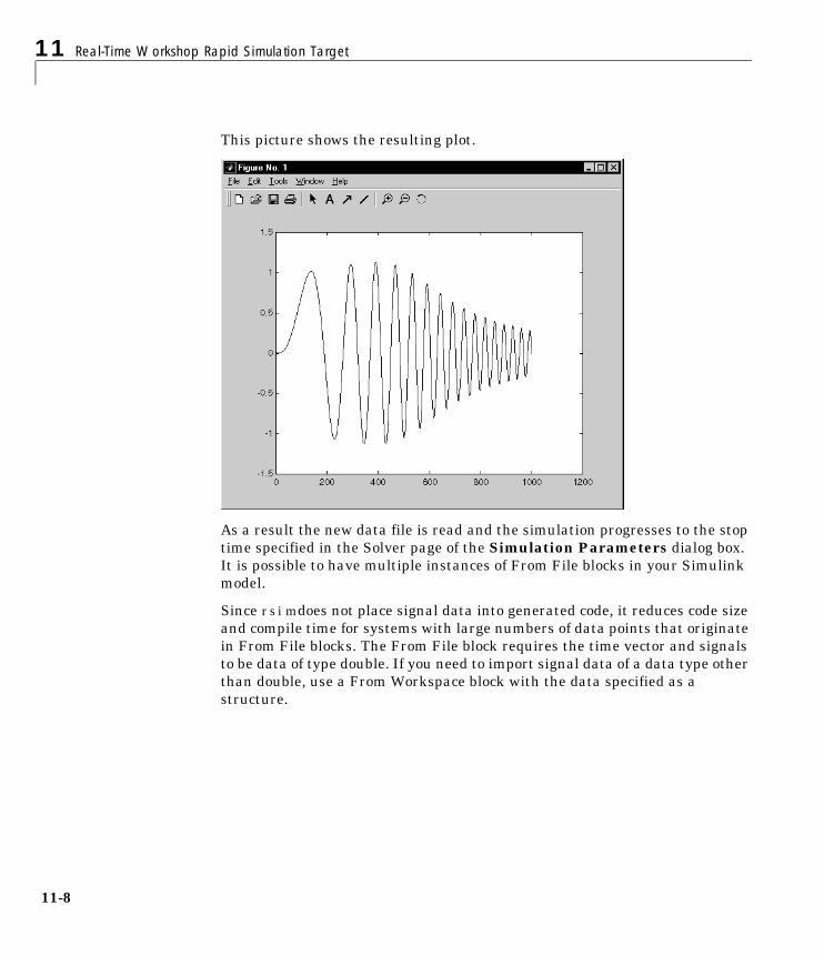
11 Real-Time Workshop Rapid Simulation Target
11-8
This picture shows the resulting plot.
As a result the new data file is read and the simulation progresses to the stoptime specified in the Solver page of the Simulation Parameters dialog box.It is possible to have multiple instances of From File blocks in your Simulinkmodel.
Since rsim does not place signal data into generated code, it reduces code sizeand compile time for systems with large numbers of data points that originatein From File blocks. The From File block requires the time vector and signalsto be data of type double. If you need to import signal data of a data type otherthan double, use a From Workspace block with the data specified as astructure.

Building for the Rapid Simulation Target
11-9
The workspace data must be in the format
variable.timevariable.signals.values
If you have more than one signal, the format must be
variable.timevariable.signals(1).valuesvariable.signals(2).values
Specifying a New Output Filename for the SimulationIf you have specified Save to Workspace options (that is, checked Time,States, Outputs, or Final States check boxes on the Workspace I/O page of theSimulation Parameters dialog box), the default is to save simulation loggingresults to the file model.mat. You can now specify a replacement filename forsubsequent simulations. In the case of the model rsimtfdemo, by typing
!rsimtfdemo
at the MATLAB prompt, a simulation runs and data is normally saved torsimtfdemo.mat.
!rsimtfdemocreated rsimtfdemo.mat
You can specify a new output filename for data logging by typing
!rsimtfdemo -o sim1.mat
In this case, the set of parameters provided at the time of code generation,including any From File block data, is run. You can combine a variety of rsimflags to provide new data, parameters, and output files to your simulation.Note that the MAT-file containing data for the From File blocks is required.This differs from the grt operation, which inserts MAT-file data directly intothe generated C code that is then compiled and linked as an executable. Incontrast, rsim allows you to provide new or replacement data sets for eachsuccessive simulation. A MAT-file containing From File or From Workspacedata must be present, if any From File or From Workspace blocks exist in yourmodel.
11 Real-Time Workshop Rapid Simulation Target
11-10
Changing Block Parameters for an rsim SimulationOnce you have altered one or more parameter in the Simulink block diagram,you can extract the parameter vector, rtP, for the entire model. The rtP vector,along with a model checksum, can then be saved to a MATLAB MAT-file. ThisMAT-file can be read in directly by the stand-alone rsim executable, allowingyou to replace the entire parameter vector quickly, for running studies ofvariations of parameter values where you are adjusting model parameters orcoefficients or importing new data for use as input signals.
The model checksum provides a safety check to ensure that any parameterchanges are only applied to rsim models that have the same model structure.If any block is deleted, or a new block added, then when generating a new rtPvector, the new checksum will no longer match the original checksum. rsimwilldetect this incompatibility in parameter vectors and exit to avoid returningincorrect simulation results. In this case, where model structure has changed,you must regenerate the code for the model.
The rsim target allows you to alter any model parameter, including parametersthat include side-effects functions. An example of a side-effects function is asimple Gain block that includes the following parameter entry in a dialog box.
gain value: 2 * a
In general, the Real-Time Workshop evaluates side-effects functions prior togenerating code. The generated code for this example retains only one memorylocation entry, and the dependence on parameter a is no longer visible in thegenerated code. The rsim target overcomes the problem of handling side-effectsfunctions by replacing the entire parameter structure, rtP. You must createthis new structure by using rsimgetrtp.m. and then save it in a MAT-file. Forthe rsimtfdemo example, type
zeta = .2;myrtp = rsimgetrtp('modelname');save myparamfile myrtp;
at the MATLAB prompt.
In turn, rsim can read the MAT-file and replace the entire rtP structurewhenever you need to change one or more parameters — without recompilingthe entire model.
For example, assume that you have changed one or more parameters in yourmodel, generated the new rtP vector, and saved rtP to a new MAT-file called

Building for the Rapid Simulation Target
11-11
myparamfile.mat. In order to run the same rsimtfdemo model and use thesenew parameter values, execute the model by typing
!rsimtfdemo -p myparamfile.matload rsimtfdemo plot(rt_yout)
Note that the p is lower-case and represents “Parameter file.”
Specifying a New Stop Time for an rsim SimulationIf a new stop time is not provided, the simulation will run until reaching thevalue specified in the Solver page at the time of code generation. You canspecify a new stop time value as follows.
!rsimtfdemo -s 6.0
In this case, the simulation will run until it reaches 6.0 seconds. At this pointit will stop and log the data according to the MAT-file data logging rules asdescribed above.
If your model includes From File blocks that also include a time vector in thefirst row of the time and signal matrix, the end of the simulation is stillregulated by the original setting in the Solver page of the SimulationParameters dialog box or from the -s option as described above. However, ifthe simulation time exceeds the end points of the time and signal matrix (thatis, if the final time is greater than the final time value of the data matrix), thenthe signal data will be extrapolated out to the final time value as specifiedabove.
Specifying New Output Filenames for To File BlocksIn much the same way as you can specify a new system output filename, youcan also provide new output filenames for data saved from one or more To Fileblocks. This is done by specifying the original filename at the time of codegeneration with a new name as follows.
!mymodel -t original.mat=replacement.mat
In this case, assume that the original model wrote data to the output file calledoriginal.mat. Specifying a new filename forces rsim to write to the filereplacement.mat. This technique allows you to avoid over-writing an existingsimulation run.
11 Real-Time Workshop Rapid Simulation Target
11-12
Simulation PerformanceIt is not possible to predict accurately the simulation speedup of an rsimsimulation compared to a standard Simulink simulation. Performance willvary. Larger simulations have achieved speed improvements of up to 10 timesfaster than standard Simulink simulations. Some models may not show anynoticeable improvement in simulation speed. The only way to determinespeedup is to time your standard Simulink simulation and then compare itsspeed with the associated rsim simulation.
Batch and Monte Carlo SimulationsThe rsim target is intended to be used for batch simulations in whichparameters and/or input signals are varied for each new simulation. Newoutput filenames allow you run new simulations without over-writing priorsimulation results. A simple example of such a set of batch simulations can berun by creating a .bat file for use under Microsoft Windows 95 or Windows NT.
This simple file (for Windows 95 or Windows NT) is created with any text editorand executed by typing the filename, for example, mybatch, where the name ofthe text file is mybatch.bat.
rsimtfdemo -f rsimtfdemo.mat=run1.mat -o results1.mat -s 10.0rsimtfdemo -f rsimtfdemo.mat=run2.mat -o results2.mat -s 10.0rsimtfdemo -f rsimtfdemo.mat=run3.mat -o results3.mat -s 10.0rsimtfdemo -f rsimtfdemo.mat=run4.mat -o results4.mat -s 10.0
In this case, batch simulations are run using the four sets of input data in filesrun1.mat, run2.mat, and so on. rsim saves the data to the corresponding filesspecified after the -o option.
The variable names containing simulation results in each of these files areidentical. Therefore, loading consecutive sets of data without renaming thedata once it is in the MATLAB workspace will result in over-writing the priorworkspace variable with new data. If you want to avoid over-writing, you cancopy the result to a new MATLAB variable prior to loading the next set of data.
You can also write M-file scripts to create new signals, and new parameterstructures, as well as to save data and perform batch runs using the bangcommand (!).
For additional insight into the rapid simulation target, explore rsimdemo1 andrsimdemo2, located in matlabroot/toolbox/rtw/rtwdemos. These examples

Building for the Rapid Simulation Target
11-13
demonstrate how rsim can be called repeatedly within an M-file for MonteCarlo simulations.

11 Real-Time Workshop Rapid Simulation Target
11-14
12Targeting Tornado forReal-Time Applications
Introduction . . . . . . . . . . . . . . . . . . . . 12-2Confirming Your Tornado Setup Is Operational . . . . . . 12-2VxWorks Library . . . . . . . . . . . . . . . . . . . 12-3
Run-Time Architecture Overview . . . . . . . . . . 12-5Parameter Tuning and Monitoring . . . . . . . . . . . 12-5Run-Time Structure . . . . . . . . . . . . . . . . . 12-8
Implementation Overview . . . . . . . . . . . . . 12-12Adding Device Driver Blocks . . . . . . . . . . . . . 12-14Configuring the Template Makefile . . . . . . . . . . 12-14Tool Locations . . . . . . . . . . . . . . . . . . . 12-15Building the Program . . . . . . . . . . . . . . . . 12-15Downloading and Running the Executable
Interactively . . . . . . . . . . . . . . . . . 12-19
12 Targeting Tornado for Real-Time Applications
12-2
This chapter contains the following topics:
• Introduction. Overview of the Tornado (VxWorks) Real-Time Target andthe VxWorks Support library.
• Run-Time Architecture Overview. Single- and multitasking architectureand host/target communications.
• Implementation Overview. Designing, implementing and running aVxWorks-based real-time program using the Real-Time Workshop.
Introduction
12-3
IntroductionThis chapter describes how to create real-time programs for execution underVxWorks, which is part of the Tornado environment.
The VxWorks real-time operating system is available from Wind RiverSystems, Inc. It provides many UNIX-like features and comes bundled with acomplete set of development tools.
Note Tornado is an integrated environment consisting of VxWorks (ahigh-performance real-time operating system), application building tools(compiler, linker, make, and archiver utilities), and interactive developmenttools (editor, debugger, configuration tool, command shell, and browser).
This chapter discusses the run-time architecture of VxWorks-based real-timeprograms generated by the Real-Time Workshop and provides specificinformation on program implementation. Topics covered include:
• Configuring device driver blocks and makefile templates
• Building the program
• Downloading the object file to the VxWorks target
• Executing the program on the VxWorks target
• Using Simulink external mode to change model parameters and downloadthem to the executing program on the VxWorks target
• Using the StethoScope data acquisition and graphical monitoring tool, whichis available as an option with VxWorks. It allows you to access the output ofany block in the model (in the real-time program) and display the data on thehost.
Confirming Your Tornado Setup Is OperationalBefore beginning, you must install and configure Tornado on your host andtarget hardware, as discussed in the Tornado documentation. You should thenrun one of the VxWorks demonstration programs to ensure you can boot yourVxWorks target and download object files to it. See the Tornado User’s Guidefor additional information about installation and operation of VxWorks andTornado products.
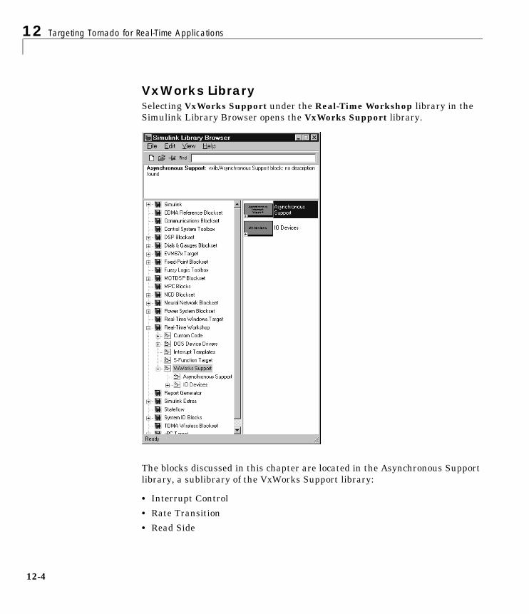
12 Targeting Tornado for Real-Time Applications
12-4
VxWorks LibrarySelecting VxWorks Support under the Real-Time Workshop library in theSimulink Library Browser opens the VxWorks Support library.
The blocks discussed in this chapter are located in the Asynchronous Supportlibrary, a sublibrary of the VxWorks Support library:
• Interrupt Control
• Rate Transition
• Read Side
Introduction
12-5
• Task Synchronization
• Write Side
A second sublibrary, the IO Devices library, contains support for these drivers:
• Matrix MS-AD12
• Matrix MS-DA12
• VME Microsystems VMIVM-3115-1
• Xycom XVME-500/590
• Xycom XVME-505/595
Each of these blocks has online help available through the Help button on theblock’s dialog box. Refer to the Tornado User’s Guide for detailed informationon these blocks.
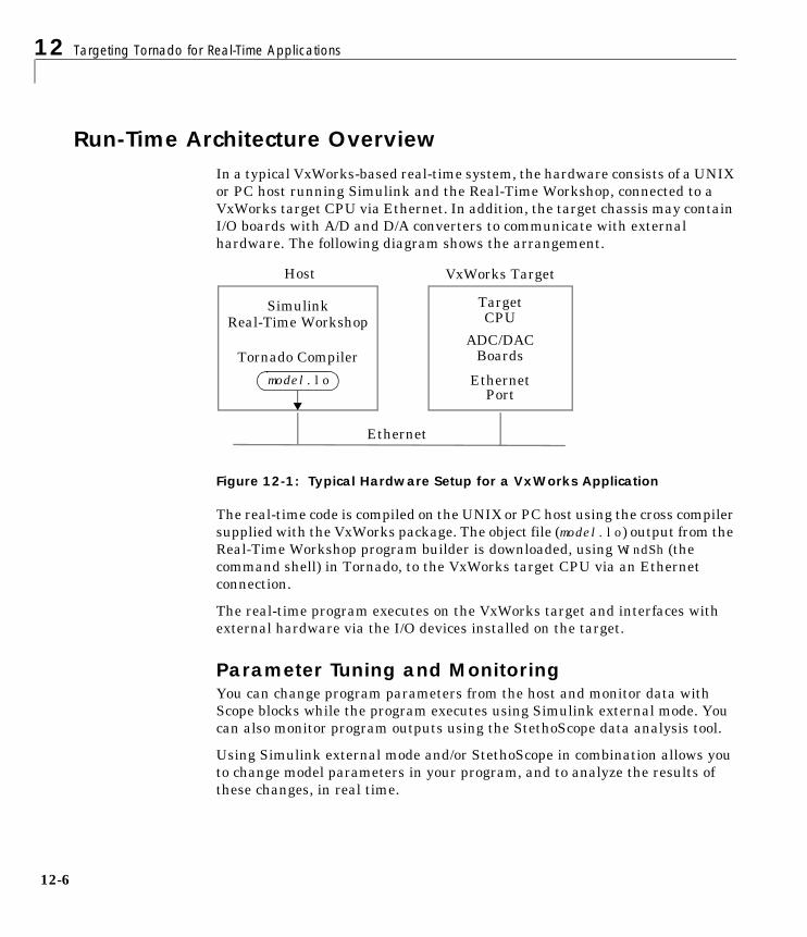
12 Targeting Tornado for Real-Time Applications
12-6
Run-Time Architecture OverviewIn a typical VxWorks-based real-time system, the hardware consists of a UNIXor PC host running Simulink and the Real-Time Workshop, connected to aVxWorks target CPU via Ethernet. In addition, the target chassis may containI/O boards with A/D and D/A converters to communicate with externalhardware. The following diagram shows the arrangement.
Figure 12-1: Typical Hardware Setup for a VxWorks Application
The real-time code is compiled on the UNIX or PC host using the cross compilersupplied with the VxWorks package. The object file (model.lo) output from theReal-Time Workshop program builder is downloaded, using WindSh (thecommand shell) in Tornado, to the VxWorks target CPU via an Ethernetconnection.
The real-time program executes on the VxWorks target and interfaces withexternal hardware via the I/O devices installed on the target.
Parameter Tuning and MonitoringYou can change program parameters from the host and monitor data withScope blocks while the program executes using Simulink external mode. Youcan also monitor program outputs using the StethoScope data analysis tool.
Using Simulink external mode and/or StethoScope in combination allows youto change model parameters in your program, and to analyze the results ofthese changes, in real time.
VxWorks Target
Ethernet
Host
SimulinkReal-Time Workshop
TargetCPU
EthernetPort
ADC/DACBoards
model.lo
Tornado Compiler
Run-Time Architecture Overview
12-7
External ModeSimulink external mode provides a mechanism to download new parametervalues to the executing program and to monitor signals in your model. In thismode, the external link MEX-file sends a vector of new parameter values to thereal-time program via the network connection. These new parameter valuesare sent to the program whenever you make a parameter change withoutrequiring a new code generation or build iteration.
You can use the BlockIOSignals code generation option to monitor signals inVxWorks. See “Interfacing Parameters and Signals” on page 17-65 for furtherinformation and example code.
The real-time program (executing on the VxWorks target) runs a low prioritytask that communicates with the external link MEX-file and accepts the newparameters as they are passed into the program.
Communication between Simulink and the real-time program is accomplishedusing the sockets network API. This implementation requires an Ethernetnetwork that supports TCP/IP. See Chapter 5, “External Mode” for moreinformation on external mode.
Changes to the block diagram structure (for example, adding or removingblocks) require generation of model and execution of the build process.
Configuring VxWorks to Use SocketsIf you want to use Simulink external mode with your VxWorks program, youmust configure your VxWorks kernel to support sockets by including theINCLUDE_NET_INIT, INCLUDE_NET_SHOW, and INCLUDE_NETWORK options in yourVxWorks image. For more information on configuring your kernel, see theVxWorks Programmer’s Guide.
Before using external mode, you must ensure that VxWorks can properlyrespond to your host over the network. You can test this by using the hostcommand
ping <target_name>
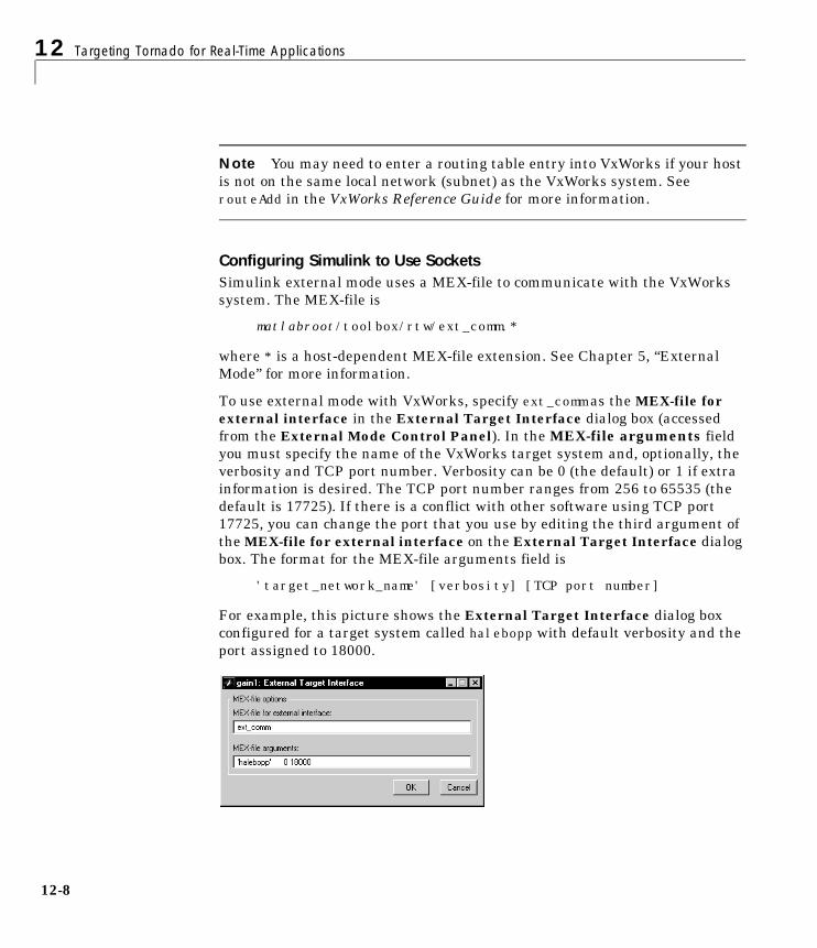
12 Targeting Tornado for Real-Time Applications
12-8
Note You may need to enter a routing table entry into VxWorks if your hostis not on the same local network (subnet) as the VxWorks system. SeerouteAdd in the VxWorks Reference Guide for more information.
Configuring Simulink to Use SocketsSimulink external mode uses a MEX-file to communicate with the VxWorkssystem. The MEX-file is
matlabroot/toolbox/rtw/ext_comm.*
where * is a host-dependent MEX-file extension. See Chapter 5, “ExternalMode” for more information.
To use external mode with VxWorks, specify ext_comm as the MEX-file forexternal interface in the External Target Interface dialog box (accessedfrom the External Mode Control Panel). In the MEX-file arguments fieldyou must specify the name of the VxWorks target system and, optionally, theverbosity and TCP port number. Verbosity can be 0 (the default) or 1 if extrainformation is desired. The TCP port number ranges from 256 to 65535 (thedefault is 17725). If there is a conflict with other software using TCP port17725, you can change the port that you use by editing the third argument ofthe MEX-file for external interface on the External Target Interface dialogbox. The format for the MEX-file arguments field is
'target_network_name' [verbosity] [TCP port number]
For example, this picture shows the External Target Interface dialog boxconfigured for a target system called halebopp with default verbosity and theport assigned to 18000.
Run-Time Architecture Overview
12-9
StethoScopeWith StethoScope, you can access the output of any block in the model (in thereal-time program) and display this data on a host. Signals are installed inStethoScope by the real-time program using the BlockIOSignals datastructure (See “Interfacing Parameters and Signals” on page 17-65 forinformation on BlockIOSignals), or interactively from the WindSh while thereal-time program is running. To use StethoScope interactively, see theStethoScope User’s Manual.
To use StethoScope you must specify the proper options with the buildcommand. See “Code Generation Options” on page 12-18 for information onthese options.
Run-Time StructureThe real-time program executes on the VxWorks target while Simulink andStethoScope execute on the same or different host workstations. Both Simulinkand StethoScope require tasks on the VxWorks target to handlecommunication.
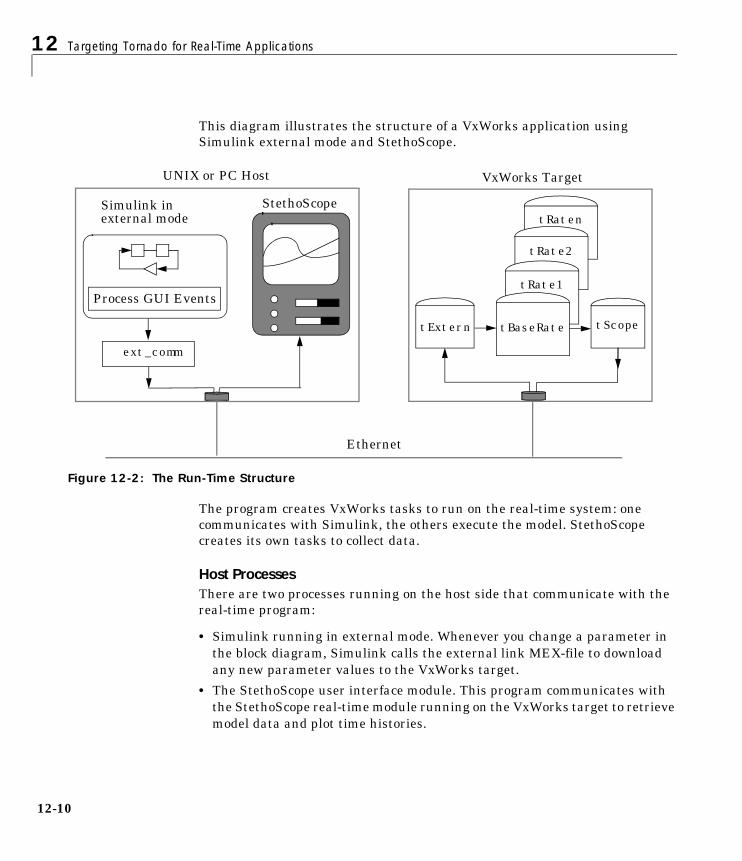
12 Targeting Tornado for Real-Time Applications
12-10
This diagram illustrates the structure of a VxWorks application usingSimulink external mode and StethoScope.
Figure 12-2: The Run-Time Structure
The program creates VxWorks tasks to run on the real-time system: onecommunicates with Simulink, the others execute the model. StethoScopecreates its own tasks to collect data.
Host ProcessesThere are two processes running on the host side that communicate with thereal-time program:
• Simulink running in external mode. Whenever you change a parameter inthe block diagram, Simulink calls the external link MEX-file to downloadany new parameter values to the VxWorks target.
• The StethoScope user interface module. This program communicates withthe StethoScope real-time module running on the VxWorks target to retrievemodel data and plot time histories.
tRaten
tRate2
tRate1
tExtern tBaseRate tScope
Simulink in StethoScope
Process GUI Events
ext_comm
external mode
Ethernet
UNIX or PC Host VxWorks Target
Run-Time Architecture Overview
12-11
VxWorks TasksYou can run the real-time program in either singletasking or multitaskingmode. The code for both modes is located in
matlabroot/rtw/c/tornado/rt_main.c
The Real-Time Workshop compiles and links rt_main.c with the model codeduring the build process.
Singletasking. By default, the model is run as one task, tSingleRate. This mayactually provide the best performance (highest base sample rate) depending onthe model.
The tSingleRate task runs at the base rate of the model and executes allnecessary code for the slower sample rates. Execution of the tSingleRate taskis normally blocked by a call to the VxWorks semTake routine. When a clockinterrupt occurs, the interrupt service routine calls the semGive routine, whichcauses the semTake call to return. Once enabled, the tSingleRate taskexecutes the model code for one time step. The loop then waits at the top byagain calling semTake. For more information about the semTake and semGiveroutines, refer to the VxWorks Reference Manual. By default, it runs at arelatively high priority (30), which allows it to execute without interruptionfrom background system activity.
Multitasking. Optionally, the model can run as multiple tasks, one for eachsample rate in the model:
• tBaseRate— This task executes the components of the model code run at thebase (highest) sample rate. By default, it runs at a relatively high priority(30), which allows it to execute without interruption from backgroundsystem activity.
• tRaten — The program also spawns a separate task for each additionalsample rate in the system. These additional tasks are named tRate1,tRate2, …, tRaten, where n is slowest sample rate in the system. Thepriority of each additional task is one lower than its predecessor (tRate1 hasa lower priority than tBaseRate).
12 Targeting Tornado for Real-Time Applications
12-12
Supporting Tasks. If you select external mode and/or StethoScope during thebuild process, these tasks will also be created:
• tExtern — This task implements the server side of a socket streamconnection that accepts data transferred from Simulink to the real-timeprogram. In this implementation, tExternwaits for a message to arrive fromSimulink. When a message arrives, tExtern retrieves it and modifies thespecified parameters accordingly.
tExtern runs at a lower priority than tRaten, the lowest priority model task.The source code for tExtern is located in matlabroot/rtw/c/src/ext_svr.c.
• tScopeDaemon and tScopeLink — StethoScope provides its own VxWorkstasks to enable real-time data collection and display. In singletasking mode,tSingleRate collects signals; in multitasking mode, tBaseRate collects them.Both perform the collection on every base time step. The StethoScope tasksthen send the data to the host for display when there is idle time, that is,when the model is waiting for the next time step to occur. rt_main.c startsthese tasks if they are not already running.

Implementation Overview
12-13
Implementation OverviewTo implement and run a VxWorks-based real-time program using theReal-Time Workshop, you must:
• Design a Simulink model for your particular application.
• Add the appropriate device driver blocks to the Simulink model, if desired.
• Configure the tornado.tmf template makefile for your particular setup.
• Establish a connection between the host running Simulink and the VxWorkstarget via Ethernet.
• Use the automatic program builder to generate the code and the custommakefile, invoke the make command to compile and link the generated code,and load and activate the tasks required.
The figure below shows the Real-Time Workshop Tornado run-time interfacemodules and the generated code for the f14 example model.
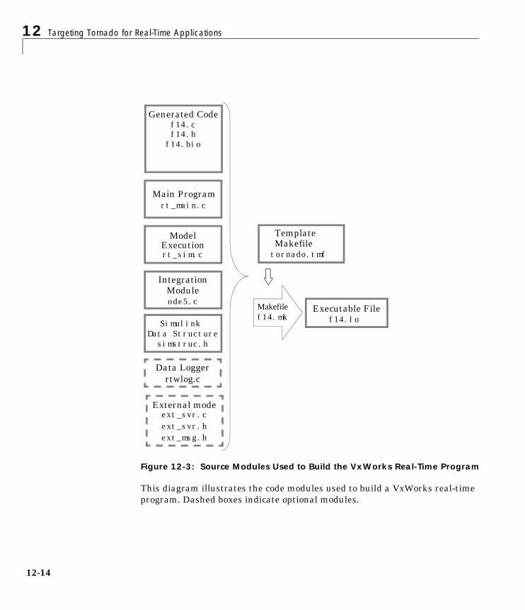
12 Targeting Tornado for Real-Time Applications
12-14
Figure 12-3: Source Modules Used to Build the VxWorks Real-Time Program
This diagram illustrates the code modules used to build a VxWorks real-timeprogram. Dashed boxes indicate optional modules.
Generated Codef14.cf14.h
rt_main.cMain Program
rt_sim.c
IntegrationModule
Model
Executable Fileode5.c
f14.lo
Execution
Makefile
TemplateMakefile
f14.mk
f14.bio
tornado.tmf
ext_svr.cExternal mode
ext_svr.hext_msg.h
Data Loggerrtwlog.c
Simulink Data Structuresimstruc.h
Implementation Overview
12-15
Adding Device Driver BlocksThe real-time program communicates with the I/O devices installed in theVxWorks target chassis via a set of device drivers. These device drivers containthe necessary code that runs on the target processor for interfacing to specificI/O devices.
To make device drivers easy to use, they are implemented as SimulinkS-functions using C code MEX-files. This means you can connect them to yourmodel like any other block and the code generator automatically includes a callto the block’s C code in the generated code.
You can also inline S-functions via the Target Language Compiler. Inliningallows you to restrict function calls to only those that are necessary for theS-function. This can greatly increase the efficiency of the S-function. For moreinformation about inlining S-functions, see Writing S-Functions and the TargetLanguage Compiler Reference Guide.
You can have multiple instances of device driver blocks in your model. SeeTargeting Real-Time Systems for more information about creating devicedrivers.
Configuring the Template MakefileTo configure the VxWorks template, tornado.tmf, you must specifyinformation about the environment in which you are using VxWorks. Thissection lists the lines in the file that you must edit.
VxWorks ConfigurationTo provide information used by VxWorks, you must specify the type of targetand the specific CPU on the target. The target type is then used to locate thecorrect cross compiler and linker for your system.
The CPU type is used to define the CPU macro which is in turn used by many ofthe VxWorks header files. Refer to the VxWorks Programmer’s Guide forinformation on the appropriate values to use.
This information is in the section labeled
#-------------- VxWorks Configuration --------------
12 Targeting Tornado for Real-Time Applications
12-16
Edit the following lines to reflect your setup.
VX_TARGET_TYPE = 68kCPU_TYPE = MC68040
Downloading ConfigurationIn order to perform automatic downloading during the build process, the targetname and host name that the Tornado target server will run on must bespecified. Modify these macros to reflect your setup.
#-------------- Macros for Downloading to Target--------------TARGET = targetnameTGTSVR_HOST = hostname
Tool LocationsIn order to locate the Tornado tools used in the build process, the followingthree macros must either be defined in the environment or specified in thetemplate makefile. Modify these macros to reflect your setup.
#-------------- Tool Locations --------------WIND_BASE = c:/TornadoWIND_HOST_TYPE = x86–win32WIND_REGISTRY = $(COMPUTERNAME)
Building the ProgramOnce you have created the Simulink block diagram, added the device drivers,and configured the makefile template, you are ready to set the build optionsand initiate the build process.
Specifying the Real-Time Build OptionsSet the real-time build options using the Solver and Real-Time Workshoppages of the Simulation Parameters dialog box. To access this dialog box,select Parameters from the Simulink Simulation menu.
In the Solver page, for models with continuous blocks, set the Type toFixed-step, the Step Size to the desired integration step size, and select theintegration algorithm. For models that are purely discrete, set the integrationalgorithm to discrete.
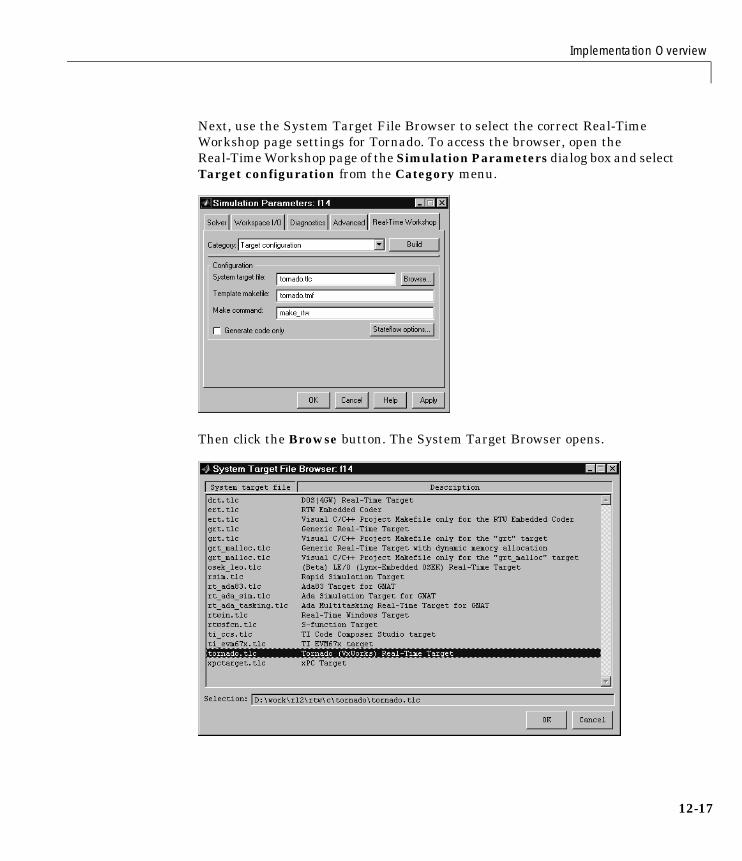
Implementation Overview
12-17
Next, use the System Target File Browser to select the correct Real-TimeWorkshop page settings for Tornado. To access the browser, open theReal-Time Workshop page of the Simulation Parameters dialog box and selectTarget configuration from the Category menu.
Then click the Browse button. The System Target Browser opens.

12 Targeting Tornado for Real-Time Applications
12-18
Select Tornado (VxWorks) Real-Time Target and click OK. This sets theTarget configuration options correctly:
• System target file — tornado.tlc
• Template makefile — tornado.tmf template, which you must configureaccording to the instructions in “Configuring the Template Makefile” on page12-15. (You can rename this file; simply change the dialog box accordingly.)
• Make command — make_rtw
You can optionally inline parameters for the blocks in the C code, which canimprove performance. Inlining parameters is not allowed when using externalmode.
Code Generation Options. To specify code generation options specific to Tornado,open the Real-Time Workshop page and select Tornado code generationoptions from the Category menu.
The Real-Time Workshop provides flags that set the appropriate macros in thetemplate makefile, causing any necessary additional steps to be performedduring the build process.
The flags and switches are as follows:
• MAT-file logging: Select this option to enable data logging during programexecution. The program will create a file named model.mat at the end of
Implementation Overview
12-19
program execution; this file will contain the variables that you specified inthe Solver page of the Simulation Parameters dialog box.
Real-Time Workshop adds a prefix or suffix to the names of the Solver pagevariables that you select for logging. The MAT-file variable name modifiermenu lets you select the prefix or suffix.
By default, the MAT-file is created in the root directory of the current defaultdevice in VxWorks. This is typically the host file system that VxWorks wasbooted from. Other remote file systems can be used as a destination for theMAT-file using rsh or ftp network devices or NFS. See the VxWorksProgrammer’s Guide for more information. If a device or filename other thanthe default is desired, add "-DSAVEFILE=filename" to the OPTS flag to themake command. For example,
make_rtw OPTS="-DSAVEFILE=filename"
• External mode: Select this option to enable the use of external mode in thegenerated executable. You can optionally enable a verbose mode of externalmode by appending -DVERBOSE to the OPTS flag in the make command. Forexample,
make_rtw OPTS="-DVERBOSE"
causes parameter download information to be printed to the console of theVxWorks system.
• Code format: Selects RealTime or RealTimeMalloc code generation format.
• StethoScope: Select this option to enable the use of StethoScope with thegenerated executable. When starting rt_main, there are two command linearguments that control the block names used by StethoScope; you can usethem when starting the program on VxWorks. See the section, “Running theProgram” on page 12-21 for more information on these arguments.
• Download to VxWorks target: Enables automatic downloading of thegenerated program.
Additional options are available on the Real-Time Workshop page. See “Usingthe Real-Time Workshop Page” on page 3-4 for information.
Initiating the BuildTo build the program, click on the Build button in the Real-Time Workshoppage of the Simulation parameters dialog. The resulting object file is namedwith the .lo extension (which stands for loadable object). This file has been
12 Targeting Tornado for Real-Time Applications
12-20
compiled for the target processor using the cross compiler specified in themakefile. If automatic downloading (Download to VxWorks target) is enabledin the Tornado code generation options, the target server is started and theobject file is downloaded and started on the target. If StethoScope was checkedon the Tornado code generation options, you can now start StethoScope onthe host. The StethoScope object files, libxdr.so, libutilstssip.so, andlibscope.so, will be loaded on the VxWorks target by the automatic download.See the StethoScope User’s Manual for more information.
Downloading and Running the Executable InteractivelyIf automatic downloading is disabled, you must use the Tornado tools tocomplete the process. This involves three steps:
1 Establishing a communication link to transfer files between the host and theVxWorks target
2 Transferring the object file from the host to the VxWorks target
3 Running the program
Connecting to the VxWorks TargetAfter completing the build process, you are ready to connect the hostworkstation to the VxWorks target. The first step is starting the target serverthat is used for communication between the Tornado tools on the host and thetarget agent on the target. This is done either from the DOS command line orfrom within the Tornado development environment. From the DOS commandline use
tgtsvr target_network_name
Downloading the Real-Time ProgramTo download the real-time program, use the VxWorks ld routine from withinWindSh. WindSh (wind shell) can also be run from the command line or fromwithin the Tornado development environment. (For example, if you want todownload the file vx_equal.lo, which is in the /home/my_working_dirdirectory, use the following commands at the WindSh prompt.

Implementation Overview
12-21
cd "/home/my_working_dir"ld <vx_equal.lo
You will also need to load the StethoScope libraries if the StethoScope optionwas selected during the build. The Tornado User’s Guide describes the ldlibrary routine.
Running the ProgramThe real-time program defines a function, rt_main(), that spawns the tasks toexecute the model code and communicate with Simulink (if you selectedexternal mode during the build procedure.) It also initializes StethoScope if youselected this option during the build procedure.
The rt_main function is defined in the rt_main.c application module. Thismodule is located in the matlabroot/rtw/c/tornado directory.
The rt_main function takes six arguments, and is defined by the followingANSI C function prototype.
SimStruct *rt_main(void (*model)(SimStruct *),char *optStr, char *scopeInstallString,int scopeFullNames,int priority,int TCPport);
Table 12-1 lists the arguments to this function.

12 Targeting Tornado for Real-Time Applications
12-22
Table 12-1: Arguments to the rt_main simStruct
Argument Description
model A pointer to the entry point function in the generated code. Thisfunction has the same name as the Simulink model. It registers thelocal functions that implement the model code by adding functionpointers to the model’s SimStruct. See Chapter 6, “ProgramArchitecture” for more information.
optStr The options string used to specify a stop time (-tf) and whether to wait(-w) in external mode for a message from Simulink before starting thesimulation. An example options string is
"-tf 20 -w"
The -tf option overrides the stop time that was set during codegeneration. If the value of the -tf option is inf, the program runsindefinitely.
scopeInstallString A character string that determines which signals are installed toStethoScope. Possible values are:
• NULL — Install no signals. This is the default value.
• "*" — Install all signals.
• "[A-Z]*" — Install signals from blocks whose names start with anuppercase letter.
Specifying any other string installs signals from blocks whose namesstart with that string.
scopeFullNames This argument determines whether StethoScope uses full hierarchicalblock names for the signals it accesses or just the individual blockname. Possible values are:
• 1 Use full block names.
• 0 Use individual block names. This is the default value.
It is important to use full block names if your program has multipleinstances of a model or S-function.
Implementation Overview
12-23
Passing optStr Via the Template Makefile. You can also pass the -w and -tf options(see optStr in Table 12-1) to rt_main by using the PROGRAM_OPTS macro intornado .tmf. PROGRAM_OPTS passes a string of the form
-opt1 val1 -opt2 val2
For example, the following sets an infinite stop time and instructs the programto wait for a message from Simulink before starting the simulation.
PROGRAM_OPTS = "-tf inf -w”
Calling rt_main. To begin program execution, call rt_main from WindSh. Forexample,
sp(rt_main, vx_equal, "-tf 20 -w", "∗", 0, 30, 17725)
• Begins execution of the vx_equal model
• Specifies a stop time of 20 seconds
• Provides access to all signals (block outputs) in the model by StethoScope
• Uses only individual block names for signal access (instead of thehierarchical name)
• Uses the default priority (30) for the tBaseRate task
• Uses TCP port 17725, the default
priority The priority of the program’s highest priority task (tBaseRate). Notspecifying any value (or specifying a value of zero) assigns tBaseRateto the default priority, 30.
TCPport The port number that the external mode sockets connection shoulduse. The valid range is 256 to 65535. When nothing is specified, theport number defaults to 17725.
Table 12-1: Arguments to the rt_main simStruct (Continued)
Argument Description

12 Targeting Tornado for Real-Time Applications
12-24

13Targeting DOS forReal-Time Applications
Introduction . . . . . . . . . . . . . . . . . . . . 13-2DOS Device Drivers Library . . . . . . . . . . . . . . 13-2
Implementation Overview . . . . . . . . . . . . . . 13-4System Configuration . . . . . . . . . . . . . . . . . 13-5Sample Rate Limits . . . . . . . . . . . . . . . . . 13-7
Device Driver Blocks . . . . . . . . . . . . . . . 13-10Device Driver Block Library . . . . . . . . . . . . . 13-10Configuring Device Driver Blocks . . . . . . . . . . . 13-11Adding Device Driver Blocks to the Model . . . . . . . 13-16
Building the Program . . . . . . . . . . . . . . . 13-17Running the Program . . . . . . . . . . . . . . . . 13-18
13 Targeting DOS for Real-Time Applications
13-2
IntroductionThis section provides information on using the Real-Time Workshop in a DOSenvironment.
Note The xPC Target and the Real-Time Windows Target providesignificantly greater capabilities than does the DOS target. We recommenduse of these targets for real-time development on PC platforms. The DOStarget is provided only as an unsupported example. Also, note that the DOStarget requires the Watcom C compiler. See “A Note on the Watcom Compiler”on page 13-6.
This chapter includes a discussion of:
• DOS-based Real-Time Workshop applications
• Supported compilers and development tools
• Device driver blocks — adding them to your model and configuring them foruse with your hardware
• Building the program
The DOS target creates an executable for DOS, using Watcom for DOS. Theexecutable runs on a computer running the DOS operating system. It will notrun under the Microsoft Windows DOS command prompt. This executableinstalls interrupt service routines and effectively takes over the computer,which allows the generated code to run in real time. If you want to run thegenerated code in real time under Microsoft Windows, you should use theReal-Time Windows Target. See the Real-Time Windows Target User’s Guidefor more information about this product.
DOS Device Drivers LibraryThe Real-Time Workshop provides DOS-compatible analog and digital I/Odevice driver blocks in the DOS Device Drivers library. Select DOS DeviceDrivers under the Real-Time Workshop library in the Simulink LibraryBrowser to open the DOS Device Drivers library.
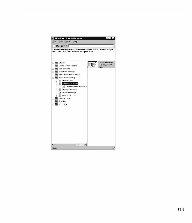
13-3
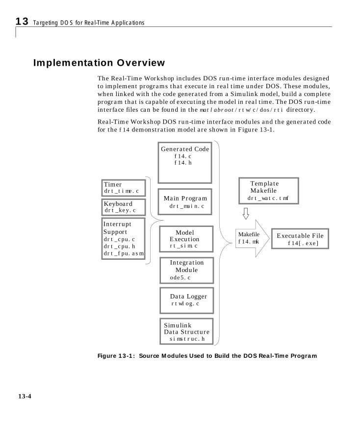
13 Targeting DOS for Real-Time Applications
13-4
Implementation OverviewThe Real-Time Workshop includes DOS run-time interface modules designedto implement programs that execute in real time under DOS. These modules,when linked with the code generated from a Simulink model, build a completeprogram that is capable of executing the model in real time. The DOS run-timeinterface files can be found in the matlabroot/rtw/c/dos/rti directory.
Real-Time Workshop DOS run-time interface modules and the generated codefor the f14 demonstration model are shown in Figure 13-1.
Figure 13-1: Source Modules Used to Build the DOS Real-Time Program
Generated Codef14.cf14.h
drt_main.cMain Program
rt_sim.c
IntegrationModule
Model
Data Structuresimstruc.h
Executable File
ode5.c
f14[.exe]Execution
Data Loggerrtwlog.c
Makefile
TemplateMakefile
f14.mk
Simulink
drt_watc.tmfdrt_time.cTimer
drt_key.cKeyboard
InterruptSupportdrt_cpu.cdrt_cpu.hdrt_fpu.asm
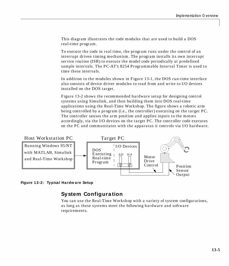
Implementation Overview
13-5
This diagram illustrates the code modules that are used to build a DOSreal-time program.
To execute the code in real time, the program runs under the control of aninterrupt driven timing mechanism. The program installs its own interruptservice routine (ISR) to execute the model code periodically at predefinedsample intervals. The PC-AT’s 8254 Programmable Interval Timer is used totime these intervals.
In addition to the modules shown in Figure 13-1, the DOS run-time interfacealso consists of device driver modules to read from and write to I/O devicesinstalled on the DOS target.
Figure 13-2 shows the recommended hardware setup for designing controlsystems using Simulink, and then building them into DOS real-timeapplications using the Real-Time Workshop. The figure shows a robotic armbeing controlled by a program (i.e., the controller) executing on the target PC.The controller senses the arm position and applies inputs to the motorsaccordingly, via the I/O devices on the target PC. The controller code executeson the PC and communicates with the apparatus it controls via I/O hardware.
Figure 13-2: Typical Hardware Setup
System ConfigurationYou can use the Real-Time Workshop with a variety of system configurations,as long as these systems meet the following hardware and softwarerequirements.
I/O Devices
PositionSensorOutput
MotorDrive
DOSExecutingReal-timeProgram
Control
Target PCHost Workstation PCRunning Windows 95/NT
with MATLAB, Simulink
and Real-Time WorkshopA/D D/A
13 Targeting DOS for Real-Time Applications
13-6
Hardware RequirementsThe hardware needed to develop and run a real-time program includes:
• A workstation running Windows 95, Windows 98, or Windows NT andcapable of running MATLAB/Simulink. This workstation is the host wherethe real-time program is built.
• A PC-AT (386 or later) running DOS. This system is the target, where thereal-time program executes.
• I/O boards, which include analog to digital converter and digital to analogconverters (collectively referred to as I/O devices), on the target.
• Electrical connections from the I/O devices to the apparatus you want tocontrol (or to use as inputs and outputs to the program in the case ofhardware-in-the-loop simulations).
Once built, you can run the executable on the target hardware as a stand-aloneprogram that is independent of Simulink.
Software RequirementsThe development host must have the following software:
• MATLAB and Simulink to develop the model, and Real-Time Workshop tocreate the code for the model. You also need the run-time interface modulesincluded with the Real-Time Workshop. These modules contain the code thathandles timing, interrupts, data logging, and background tasks.
• Watcom C/C++ compiler, Version 10.6 or 11.0. (see “A Note on the WatcomCompiler” below.)
The target PC must have the following software:
• DOS4GW extender dos4gw.exe, included with your Watcom compilerpackage) must be on the search path on the DOS-targeted PC.
You can compile the generated code (i.e., the files model.c, model.h, etc.) alongwith user-written code using other compilers. However, the use of 16-bitcompilers is not recommended for any application.
A Note on the Watcom CompilerAs of this writing, the Watcom C compiler is no longer available from themanufacturer. The Real-Time Workshop continues to ship Watcom-related
Implementation Overview
13-7
target configurations at this time. However, this policy may be subject tochange in the future.
Device DriversIf your application needs to access its I/O devices on the target, then thereal-time program must contain device driver code to handle communicationwith the I/O boards. The Real-Time Workshop DOS run-time interface includessource code of the device drivers for the Keithley Metrabyte DAS-1600/1400Series I/O boards. See “Device Driver Blocks” on page 13-10 for information onhow to use these blocks.
Simulink HostThe development host must have Windows 95, Windows 98, or Windows NT torun Simulink. However, the real-time target requires only DOS, since theexecutable built from the generated code is not a Windows application. Thereal-time target will not run in a “DOS box” (i.e., a DOS window on Windows95/98/NT).
Although it is possible to reboot the host PC under DOS for real-time execution,the computer would need to be rebooted under Windows 95/NT for anysubsequent changes to the block diagram in Simulink. Since this process ofrepeated rebooting the computer is inconvenient, we recommend a second PCrunning only DOS as the real-time target.
Sample Rate LimitsProgram timing is controlled by installing an interrupt service routine thatexecutes the model code. The target PC’s CPU is then interrupted at thespecified rate (this rate is determined from the step size).
The rate at which interrupts occur is controlled by application code suppliedwith the Real-Time Workshop. This code uses the PC-AT’s 8254 Counter/Timerto determine when to generate interrupts.
The code that sets up the 8254 Timer is in drt_time.c, which is in thematlabroot\rtw\c\dos\rti directory. It is automatically linked in when youbuild the program using the DOS real-time template makefile.
The 8254 Timer is a 16-bit counter that operates at a frequency of 1.193 MHz.However, the timing module drt_time.c in the DOS run-time interface canextend the range by an additional 16 bits in software, effectively yielding a
13 Targeting DOS for Real-Time Applications
13-8
32-bit counter. This means that the slowest base sample rate your model canhave is
This corresponds to a maximum base step size of approximately one hour.
The fastest sample rate you can define is determined by the minimum valuefrom which the counter can count down. This value is 3, hence the fastestsample rate that the 8254 is capable of achieving is
This corresponds to a minimum base step size of
However, note that the above number corresponds to the fastest rate at whichthe timer can generate interrupts. It does not account for execution time for themodel code, which would substantially reduce the fastest sample rate possiblefor the model to execute in real time. Execution speed is machine dependentand varies with the type of processor and the clock rate of the processor on thetarget PC.
The slowest and fastest rates computed above refer to the base sample times inthe model. In a model with more than one sample time, you can define blocksthat execute at slower rates as long as the sample times are an integer multipleof the base sample time.
Modifying Program TimingIf you have access to an alternate timer (e.g., some I/O boards include their ownclock devices), you can replace the file drt_time.c with an equivalent file thatmakes use of the separate clock source. See the comments in drt_time.c tounderstand how the code works.
You can use your version of the timer module by redefining the TIMER_OBJSmacros with the build command. For example, in the Real-Time Workshoppage of the Simulation parameters dialog box, changing the build commandto
make_rtw TIMER_OBJS=my_timer.obj
1.1936×10 232 1–( )÷ 1
3600-------------Hz≈
1.193 106× 3÷ 4 105× Hz≈
1 4 105×÷ 2.5 10 6–× ondssec≈

Implementation Overview
13-9
replaces the file drt_time.c with my_timer.c in the list of source files used tobuild the program.

13 Targeting DOS for Real-Time Applications
13-10
Device Driver BlocksThe real-time program communicates with external hardware via a set ofdevice drivers. These device drivers contain the necessary code for interfacingto specific I/O devices.
The Real-Time Workshop includes device drivers for commercially availableKeithley Metrabyte DAS-1600/1400 Series I/O boards. These device drivers areimplemented as C MEX S-functions to interface with Simulink. This meansyou can add them to your model like any other block.
In addition, each of these S-function device drivers has a corresponding targetfile to inline the device driver in the model code. See “Creating Device Drivers”on page 17-34 for information on implementing your own device drivers.
Since the device drivers are provided as source code, you can use these devicedrivers as a template to serve a a starting point for creating custom devicedrivers for other I/O boards.
Device Driver Block LibraryThe device driver blocks for the Keithley Metrabyte DAS-1600/1400 Series I/Oboards designed for use with DOS applications are contained in a block librarycalled doslib (matlabroot\toolbox\rtw\doslib.mdl). To display this library,type
doslib
at the MATLAB prompt. This window will appear.
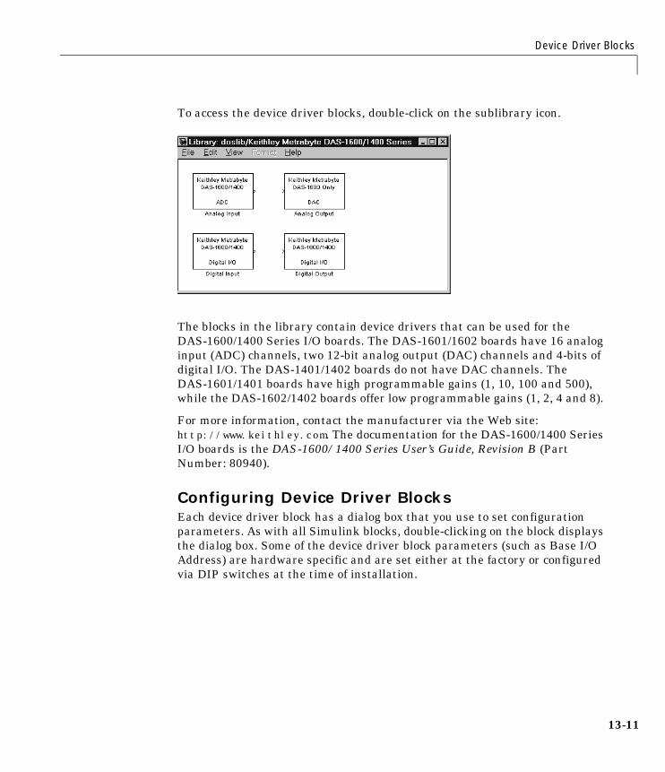
Device Driver Blocks
13-11
To access the device driver blocks, double-click on the sublibrary icon.
The blocks in the library contain device drivers that can be used for theDAS-1600/1400 Series I/O boards. The DAS-1601/1602 boards have 16 analoginput (ADC) channels, two 12-bit analog output (DAC) channels and 4-bits ofdigital I/O. The DAS-1401/1402 boards do not have DAC channels. TheDAS-1601/1401 boards have high programmable gains (1, 10, 100 and 500),while the DAS-1602/1402 boards offer low programmable gains (1, 2, 4 and 8).
For more information, contact the manufacturer via the Web site:http://www.keithley.com. The documentation for the DAS-1600/1400 SeriesI/O boards is the DAS-1600/1400 Series User’s Guide, Revision B (PartNumber: 80940).
Configuring Device Driver BlocksEach device driver block has a dialog box that you use to set configurationparameters. As with all Simulink blocks, double-clicking on the block displaysthe dialog box. Some of the device driver block parameters (such as Base I/OAddress) are hardware specific and are set either at the factory or configuredvia DIP switches at the time of installation.
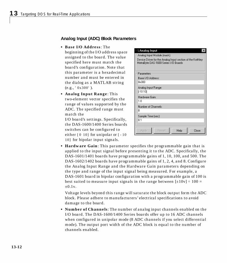
13 Targeting DOS for Real-Time Applications
13-12
Analog Input (ADC) Block Parameters
• Base I/O Address: Thebeginning of the I/O address spaceassigned to the board. The valuespecified here must match theboard’s configuration. Note thatthis parameter is a hexadecimalnumber and must be entered inthe dialog as a MATLAB string(e.g., '0x300').
• Analog Input Range: Thistwo-element vector specifies therange of values supported by theADC. The specified range mustmatch theI/O board’s settings. Specifically,the DAS-1600/1400 Series boardsswitches can be configured toeither [0 10] for unipolar or [-10 10] for bipolar input signals.
• Hardware Gain: This parameter specifies the programmable gain that isapplied to the input signal before presenting it to the ADC. Specifically, theDAS-1601/1401 boards have programmable gains of 1, 10, 100, and 500. TheDAS-1602/1402 boards have programmable gains of 1, 2, 4, and 8. Configurethe Analog Input Range and the Hardware Gain parameters depending onthe type and range of the input signal being measured. For example, aDAS-1601 board in bipolar configuration with a programmable gain of 100 isbest suited to measure input signals in the range between [±10v] ÷ 100 =±0.1v.
Voltage levels beyond this range will saturate the block output form the ADCblock. Please adhere to manufacturers’ electrical specifications to avoiddamage to the board.
• Number of Channels: The number of analog input channels enabled on theI/O board. The DAS-1600/1400 Series boards offer up to 16 ADC channelswhen configured in unipolar mode (8 ADC channels if you select differentialmode). The output port width of the ADC block is equal to the number ofchannels enabled.
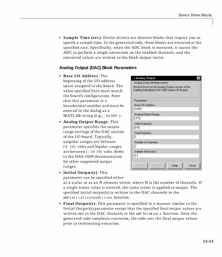
Device Driver Blocks
13-13
• Sample Time (sec): Device drivers are discrete blocks that require you tospecify a sample time. In the generated code, these blocks are executed at thespecified rate. Specifically, when the ADC block is executed, it causes theADC to perform a single conversion on the enabled channels, and theconverted values are written to the block output vector.
Analog Output (DAC) Block Parameters
• Base I/O Address: Thebeginning of the I/O addressspace assigned to the board. Thevalue specified here must matchthe board’s configuration. Notethat this parameter is ahexadecimal number and must beentered in the dialog as aMATLAB string (e.g., '0x300').
• Analog Output Range: Thisparameter specifies the outputrange settings of the DAC sectionof the I/O board. Typically,unipolar ranges are between[0 10] volts and bipolar rangesare between [-10 10] volts. Referto the DAS-1600 documentationfor other supported outputranges.
• Initial Output(s): Thisparameter can be specified eitheras a scalar or as an N element vector, where N is the number of channels. Ifa single scalar value is entered, the same scalar is applied to output. Thespecified initial output(s) is written to the DAC channels in themdlInitializeConditions function.
• Final Output(s): This parameter is specified in a manner similar to theInitial Output(s) parameter except that the specified final output values arewritten out to the DAC channels in the mdlTerminate function. Once thegenerated code completes execution, the code sets the final output valuesprior to terminating execution.
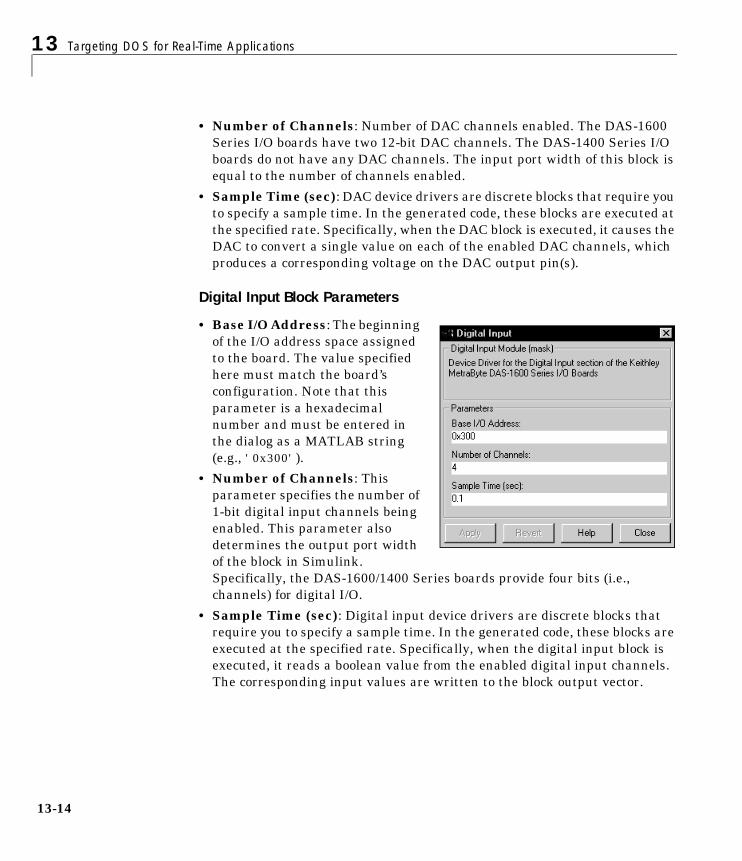
13 Targeting DOS for Real-Time Applications
13-14
• Number of Channels: Number of DAC channels enabled. The DAS-1600Series I/O boards have two 12-bit DAC channels. The DAS-1400 Series I/Oboards do not have any DAC channels. The input port width of this block isequal to the number of channels enabled.
• Sample Time (sec): DAC device drivers are discrete blocks that require youto specify a sample time. In the generated code, these blocks are executed atthe specified rate. Specifically, when the DAC block is executed, it causes theDAC to convert a single value on each of the enabled DAC channels, whichproduces a corresponding voltage on the DAC output pin(s).
Digital Input Block Parameters
• Base I/O Address: The beginningof the I/O address space assignedto the board. The value specifiedhere must match the board’sconfiguration. Note that thisparameter is a hexadecimalnumber and must be entered inthe dialog as a MATLAB string(e.g., '0x300').
• Number of Channels: Thisparameter specifies the number of1-bit digital input channels beingenabled. This parameter alsodetermines the output port widthof the block in Simulink.Specifically, the DAS-1600/1400 Series boards provide four bits (i.e.,channels) for digital I/O.
• Sample Time (sec): Digital input device drivers are discrete blocks thatrequire you to specify a sample time. In the generated code, these blocks areexecuted at the specified rate. Specifically, when the digital input block isexecuted, it reads a boolean value from the enabled digital input channels.The corresponding input values are written to the block output vector.
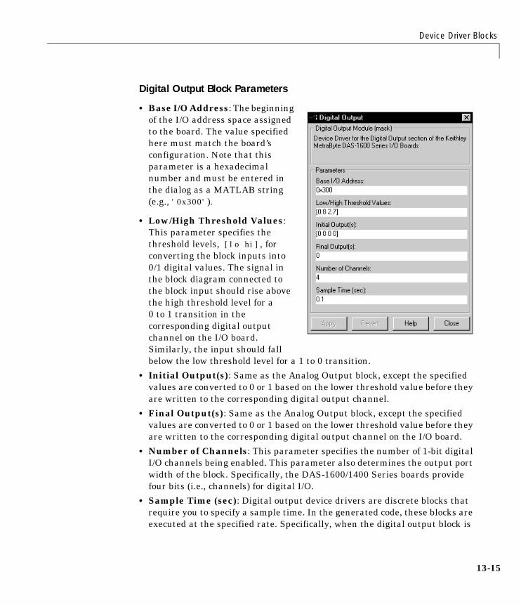
Device Driver Blocks
13-15
Digital Output Block Parameters
• Base I/O Address: The beginningof the I/O address space assignedto the board. The value specifiedhere must match the board’sconfiguration. Note that thisparameter is a hexadecimalnumber and must be entered inthe dialog as a MATLAB string(e.g., '0x300').
• Low/High Threshold Values:This parameter specifies thethreshold levels, [lo hi], forconverting the block inputs into0/1 digital values. The signal inthe block diagram connected tothe block input should rise abovethe high threshold level for a0 to 1 transition in thecorresponding digital outputchannel on the I/O board.Similarly, the input should fallbelow the low threshold level for a 1 to 0 transition.
• Initial Output(s): Same as the Analog Output block, except the specifiedvalues are converted to 0 or 1 based on the lower threshold value before theyare written to the corresponding digital output channel.
• Final Output(s): Same as the Analog Output block, except the specifiedvalues are converted to 0 or 1 based on the lower threshold value before theyare written to the corresponding digital output channel on the I/O board.
• Number of Channels: This parameter specifies the number of 1-bit digitalI/O channels being enabled. This parameter also determines the output portwidth of the block. Specifically, the DAS-1600/1400 Series boards providefour bits (i.e., channels) for digital I/O.
• Sample Time (sec): Digital output device drivers are discrete blocks thatrequire you to specify a sample time. In the generated code, these blocks areexecuted at the specified rate. Specifically, when the digital output block is
13 Targeting DOS for Real-Time Applications
13-16
executed, it causes corresponding boolean values to be output from theboard’s digital I/O channels.
Adding Device Driver Blocks to the ModelAdd device driver blocks to the Simulink block diagram as you would any otherblock — simply drag the block from the block library and insert it into themodel. Connect the ADC or Digital Input block to the model’s inputs andconnect the DAC or Digital Output block to the model’s outputs.
Including Device Driver CodeDevice driver blocks are implemented as S-functions written in C. The C codefor a device driver block is compiled as a MEX-file so that it can be called bySimulink. See the MATLAB Application Program Interface Guide forinformation on MEX-files.
The same C code can also be compiled and linked to the generated code just likeany other C-coded, S-function. However, by using the target (.tlc) file thatcorresponds to each of the C file S-functions, the device driver code is inlined inthe generated code.
The matlabroot\rtw\c\dos\devices directory contains the MEX-files, C files,and target files (.tlc) for the device driver blocks included in doslib. Thisdirectory is automatically added to your MATLAB path when you include anyof the blocks from doslib in your model.
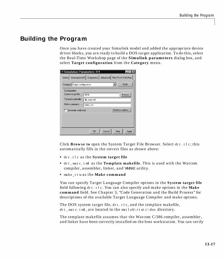
Building the Program
13-17
Building the ProgramOnce you have created your Simulink model and added the appropriate devicedriver blocks, you are ready to build a DOS target application. To do this, selectthe Real-Time Workshop page of the Simulink parameters dialog box, andselect Target configuration from the Category menu.
Click Browse to open the System Target File Browser. Select drt.tlc; thisautomatically fills in the correct files as shown above:
• drt.tlc as the System target file
• drt_watc.tmf as the Template makefile. This is used with the Watcomcompiler, assembler, linker, and WMAKE utility.
• make_rtw as the Make command
You can specify Target Language Compiler options in the System target filefield following drt.tlc. You can also specify and make options in the Makecommand field. See Chapter 3, “Code Generation and the Build Process” fordescriptions of the available Target Language Compiler and make options.
The DOS system target file, drt.tlc, and the template makefile,drt_watc.tmf, are located in the matlab\rtw\c\dos directory.
The template makefile assumes that the Watcom C/386 compiler, assembler,and linker have been correctly installed on the host workstation. You can verify

13 Targeting DOS for Real-Time Applications
13-18
this by checking the environment variable, WATCOM, which correctly points tothe directory where the Watcom files are installed.
The program builder invokes the Watcom wmake utility on the generatedmakefile, so the directory where wmake is installed must be on your path.
Running the ProgramThe result of the build process is a DOS 32-bit protected-mode executable. Thedefault name of the executable is model.exe, where model is the name of yourSimulink model. You must run this executable in DOS; you cannot run theexecutable in Windows 95/98/NT.
14Custom Code Blocks
Introduction . . . . . . . . . . . . . . . . . . . . 14-2
Custom Code Library . . . . . . . . . . . . . . . . 14-5Model Code Sublibrary . . . . . . . . . . . . . . . . 14-5Subsystem Code Sublibrary . . . . . . . . . . . . . . 14-9

14 Custom Code Blocks
14-2
IntroductionThis chapter discusses the Custom Code library, a collection of blocks thatallow you to insert custom code into the generated source code files and/orfunctions associated with your model.
The Custom Code library is part of the Real-Time Workshop library. You canaccess the Real-Time Workshop library via the Simulink Library Browser asshown in Figure 14-1. Alternatively, you can access the Real-Time Workshoplibrary by typing the command
rtwlib
at the MATLAB command prompt.
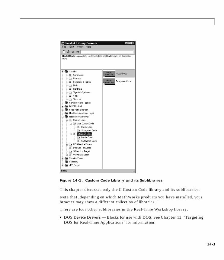
14-3
Figure 14-1: Custom Code Library and its Sublibraries
This chapter discusses only the C Custom Code library and its sublibraries.
Note that, depending on which MathWorks products you have installed, yourbrowser may show a different collection of libraries.
There are four other sublibraries in the Real-Time Workshop library:
• DOS Device Drivers — Blocks for use with DOS. See Chapter 13, “TargetingDOS for Real-Time Applications” for information.
14 Custom Code Blocks
14-4
• Interrupt Templates — A collection of blocks that you can use as templatesfor building your own asynchronous interrupts. See Chapter 15,“Asynchronous Support” for information.
• S-Function Target — The S-Function Target sublibrary contains only oneblock type, the Real-Time Workshop S-Function block. This block is intendedfor use with generated S-functions. See Chapter 10, “The S-Function Target”for more information.
• VxWorks Support — A collection of blocks that support VxWorks (Tornado).See Chapter 12, “Targeting Tornado for Real-Time Applications” forinformation on VxWorks.

Custom Code Library
14-5
Custom Code LibraryThe Custom Code library contains blocks that allow you to place your own code,in C or in Ada, inside the code generated by the Real-Time Workshop.
Figure 14-1 illustrates the hierarchy of sublibraries under the Real-TimeWorkshop library. First, the Custom Code library has two sublibraries:
• C Custom Code
• Ada Custom Code
Both the C Custom Code and Ada Custom Code libraries, in turn, haveidentically named sublibraries:
• Model Code
• Subsystem Code
Both sublibraries contain blocks that target specific files and subsystemswithin which you can place your code.
The following sections discuss the Model Code and Subsystem Codesublibraries of the C Custom Code library.
Model Code SublibraryThe Model Code sublibrary contains 10 blocks that insert custom code into thegenerated model files and functions. You can view the blocks either by:
• Expanding the Model Code sublibrary (under C Custom Code) in theSimulink Library Browser
• Right-clicking on the Model Code sublibrary icon in the right pane of theSimulink Library Browser
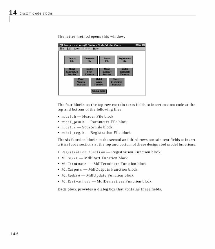
14 Custom Code Blocks
14-6
The latter method opens this window.
The four blocks on the top row contain texts fields to insert custom code at thetop and bottom of the following files:
• model.h — Header File block• model_prm.h — Parameter File block• model.c — Source File block• model_reg.h — Registration File block
The six function blocks in the second and third rows contain text fields to insertcritical code sections at the top and bottom of these designated model functions:
• Registration function — Registration Function block
• MdlStart — MdlStart Function block• MdlTerminate — MdlTerminate Function block• MdlOutputs — MdlOutputs Function block
• MdlUpdate — MdlUpdate Function block
• MdlDerivatives — MdlDerivatives Function block
Each block provides a dialog box that contains three fields.
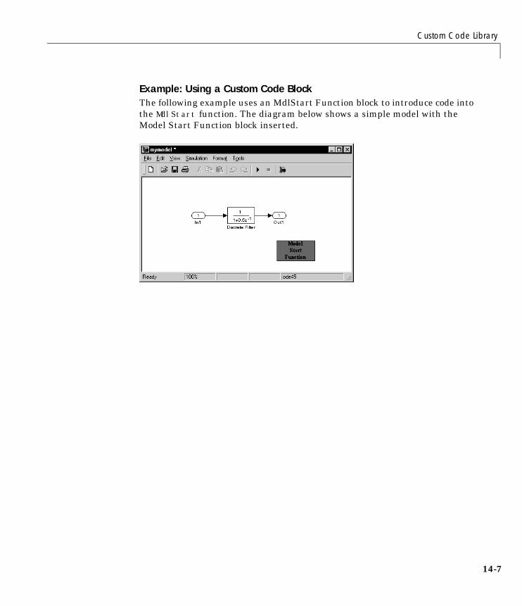
Custom Code Library
14-7
Example: Using a Custom Code BlockThe following example uses an MdlStart Function block to introduce code intothe MdlStart function. The diagram below shows a simple model with theModel Start Function block inserted.
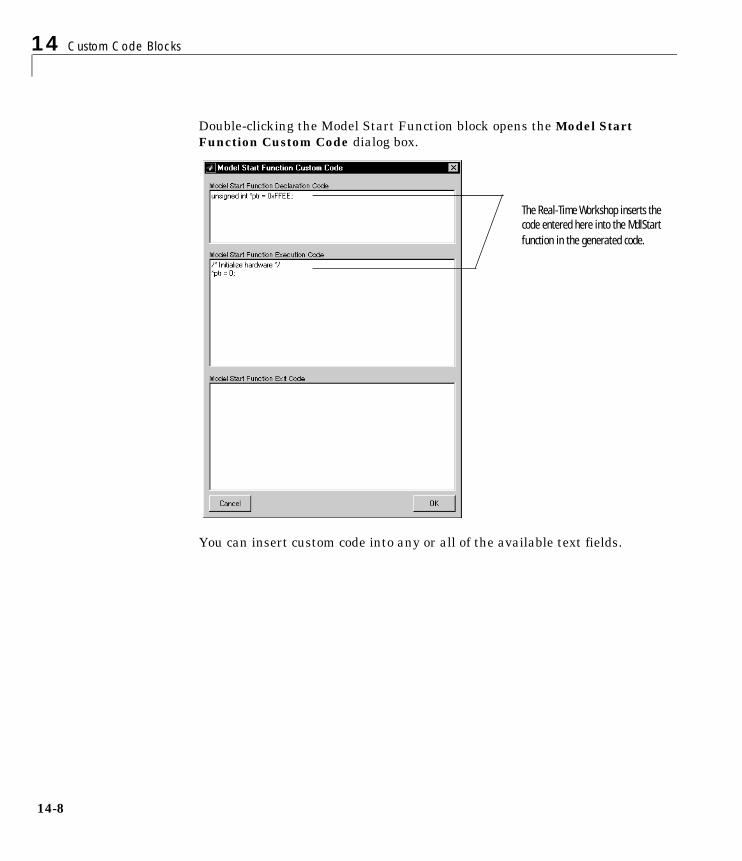
14 Custom Code Blocks
14-8
Double-clicking the Model Start Function block opens the Model StartFunction Custom Code dialog box.
You can insert custom code into any or all of the available text fields.
The Real-Time Workshop inserts the code entered here into the MdlStart function in the generated code.
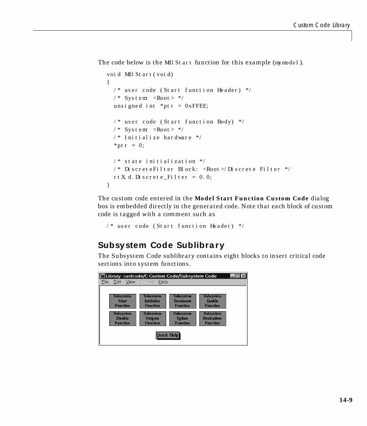
Custom Code Library
14-9
The code below is the MdlStart function for this example (mymodel).
void MdlStart(void){ /* user code (Start function Header) */ /* System: <Root> */ unsigned int *ptr = 0xFFEE;
/* user code (Start function Body) */ /* System: <Root> */ /* Initialize hardware */ *ptr = 0;
/* state initialization */ /* DiscreteFilter Block: <Root>/Discrete Filter */ rtX.d.Discrete_Filter = 0.0;}
The custom code entered in the Model Start Function Custom Code dialogbox is embedded directly in the generated code. Note that each block of customcode is tagged with a comment such as
/* user code (Start function Header) */
Subsystem Code SublibraryThe Subsystem Code sublibrary contains eight blocks to insert critical codesections into system functions.
14 Custom Code Blocks
14-10
Each of these blocks has a dialog box containing two text fields that allow youto place data at the top and the bottom of system functions. The eight blocksare:
• Subsystem Start
• Subsystem Initialize
• Subsystem Terminate
• Subsystem Enable
• Subsystem Disable
• Subsystem Outputs
• Subsystem Update
• Subsystem Derivatives
The location of the block in your model determines the location of the customcode. In other words, the code is local to the subsystem that you select. Forexample, the Subsystem Outputs block places code in mdlOutputs when thecode block resides in the root model. If the Subsystem Outputs block resides ina triggered or enabled subsystem, however, the code is placed in thesubsystem’s Outputs function.
The ordering for a triggered or enabled system is:
1 Output entry
2 Output exit
3 Update entry
4 Update exit code
15
Asynchronous Support
Introduction . . . . . . . . . . . . . . . . . . . . 15-2
Interrupt Handling . . . . . . . . . . . . . . . . . 15-5Asynchronous Interrupt Block . . . . . . . . . . . . . 15-5Task Synchronization Block . . . . . . . . . . . . . 15-12Asynchronous Buffer Block . . . . . . . . . . . . . 15-16Rate Transition Block . . . . . . . . . . . . . . . . 15-18
Creating a Customized Asynchronous Library . . . 15-20
15 Asynchronous Support
15-2
IntroductionThe Interrupt Templates are blocks that you can use as templates for buildingyour own asynchronous interrupts.
The Interrupt Templates library is part of the Real-Time Workshop library.You can access the Real-Time Workshop library via the Simulink LibraryBrowser as shown in Figure 15-1. Alternatively, you can access the Real-TimeWorkshop library by typing the command
rtwlib
at the MATLAB command prompt.
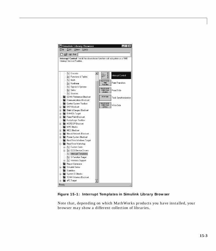
15-3
Figure 15-1: Interrupt Templates in Simulink Library Browser
Note that, depending on which MathWorks products you have installed, yourbrowser may show a different collection of libraries.
15 Asynchronous Support
15-4
Other sublibraries in the Real-Time Workshop library are:
• DOS Device Drivers: Blocks for use with DOS. See Chapter 13, “TargetingDOS for Real-Time Applications” for information.
• Custom Code Blocks: Blocks that allow you to insert custom code into thegenerated source code files and/or functions associated with your model. SeeChapter 14, “Custom Code Blocks.” for information.
• S-Function Target: The S-Function Target sublibrary contains only oneblock type, the RTW S-Function block. This block is intended for use withgenerated S-functions. See Chapter 10, “The S-Function Target” for moreinformation.
• VxWorks Support: A collection of blocks that support VxWorks (Tornado).See Chapter 12, “Targeting Tornado for Real-Time Applications” forinformation on VxWorks.
Interrupt Handling
15-5
Interrupt HandlingThe blocks in the Interrupt Templates library allow you to model synchronous/asynchronous event handling, including interrupt service routines (ISRs).These blocks include:
• Asynchronous Buffer block (read)
• Asynchronous Buffer block (write)
• Asynchronous Interrupt block
• Asynchronous Rate Transition block
• Task Synchronization block
Using these blocks, you can create models that handle asynchronous events,such as hardware generated interrupts and asynchronous read and writeoperations. The following sections discuss each of these blocks in the context ofVxWorks Tornado operating system.
Asynchronous Interrupt BlockInterrupt service routines (ISR) are realized by connecting the outputs of theVxWorks Asynchronous Interrupt block to the control input of a function-callsubsystem, the input of a VxWorks Task Synchronization block, or the input toa Stateflow chart configured for a function-call input event.
The Asynchronous Interrupt block installs the downstream (destination)function-call subsystem as an ISR and enables the specified interrupt level.The current implementation of the VxWorks Asynchronous Interrupt blocksupports VME interrupts 1-7 and uses the VxWorks system callssysIntEnable, sysIntDisable, intConnect, intLock and intUnlock. Ensurethat your target architecture (BSP) for VxWorks supports these functions.
When a function-call subsystem is connected to an Asynchronous Interruptblock output, the generated code for that subsystem becomes the ISR. For largesubsystems, this can have a large impact on interrupt response time forinterrupts of equal and lower priority in the system. As a general rule, it is bestto keep ISRs as short as possible. To do this, you should only connectfunction-call subsystems that contain few blocks.
A better solution for large systems is to use the Task Synchronization block tosynchronize the execution of the function-call subsystem to an event. The TaskSynchronization block is placed between the Asynchronous Interrupt block and
15 Asynchronous Support
15-6
the function-call subsystem (or Stateflow chart). The Asynchronous Interruptblock then installs the Task Synchronization block as the ISR, which releasesa synchronization semaphore (performs a semGive) to the function-callsubsystem and then returns. See the VxWorks Task Synchronization block formore information.
Using the Asynchronous Interrupt BlockThe Asynchronous Interrupt block has two modes that help support rapidprototyping:
• RTW mode. In RTW mode, the Asynchronous Interrupt block configures thedownstream system as an ISR and enables interrupts during model startup.You can select this mode using the Asynchronous Interrupt block dialog boxwhen generating code.
• Simulation mode. In Simulation mode, simulated Interrupt Request (IRQ)signals are routed through the Asynchronous Interrupt block’s trigger port.Upon receiving a simulated interrupt, the block calls the associated system.
You should select this mode when simulating, in Simulink, the effects of aninterrupt signal. Note that there can only be one VxWorks AsynchronousInterrupt block in a model and all desired interrupts should be configured byit.
In both RTW and Simulation mode, in the event that two IRQ signals occursimultaneously, the Asynchronous Interrupt block executes the downstreamsystems according to their priority interrupt level.
The Asynchronous Interrupt block provides these two modes to make thedevelopment and implementation of real-time systems that include ISRs easierand quicker. You can develop two models, one that includes a plant and acontroller for simulation, and one that only includes the controller for codegeneration.
Using the Library feature of Simulink, you can implement changes to bothmodels simultaneously. Figure 15-1 illustrates how changes made to the plantor controller, both of which are in a library, propagate to the models.
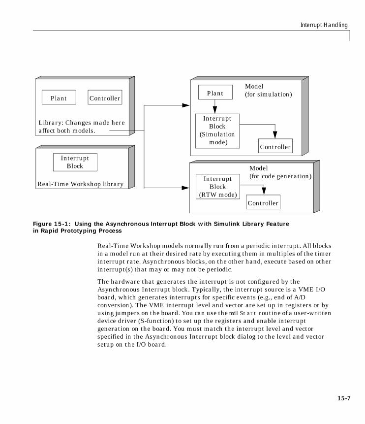
Interrupt Handling
15-7
Figure 15-1: Using the Asynchronous Interrupt Block with Simulink Library Featurein Rapid Prototyping Process
Real-Time Workshop models normally run from a periodic interrupt. All blocksin a model run at their desired rate by executing them in multiples of the timerinterrupt rate. Asynchronous blocks, on the other hand, execute based on otherinterrupt(s) that may or may not be periodic.
The hardware that generates the interrupt is not configured by theAsynchronous Interrupt block. Typically, the interrupt source is a VME I/Oboard, which generates interrupts for specific events (e.g., end of A/Dconversion). The VME interrupt level and vector are set up in registers or byusing jumpers on the board. You can use the mdlStart routine of a user-writtendevice driver (S-function) to set up the registers and enable interruptgeneration on the board. You must match the interrupt level and vectorspecified in the Asynchronous Interrupt block dialog to the level and vectorsetup on the I/O board.
Library: Changes made here
Plant Controller
InterruptBlock
Real-Time Workshop library
Plant
Controller
Controller
InterruptBlock
InterruptBlock
Model(for simulation)
Model(for code generation)
affect both models. (Simulation
(RTW mode)
mode)

15 Asynchronous Support
15-8
Asynchronous Interrupt Block ParametersThe picture below shows the VxWorks Asynchronous Interrupt block dialogbox.
Parameters associated with the Asynchronous Interrupt block are:
• Mode: In Simulation mode, the ISRs are executed nonpreemptively. If theyoccur simultaneously, signals are executed in the order specified by theirnumber (1 being the highest priority). Interrupt mapping during simulationis left to right, top to bottom. That is, the first control input signal maps tothe topmost ISR. The last control input signal maps to the bottom most ISR.
In RTW mode, the Real-Time Workshop uses vxinterrupt.tlc to realizeasynchronous interrupts in the generated code. The ISR is passed oneargument, the root SimStruct, and the Simulink definition of thefunction-call subsystem is remapped to conform with the information in theSimStruct.
• VME Interrupt Number(s): Specify the VME interrupt numbers for theinterrupts to be installed. The valid range is 1-7; for example: [4 2 5]).
• VME Interrupt Vector Offset Number(s): The Real-Time Workshop uses thisnumber in the call to intConnect(INUM_TO_IVEC(#),...). You shouldspecify a unique vector offset number for each interrupt number.
• Preemption Flag(s): By default, higher priority interrupts can preempt lowerpriority interrupts in VxWorks. If desired, you can lock out interrupts during

Interrupt Handling
15-9
the execution of a ISR by setting the preemption flag to 0. This causesintLock() and intUnlock() calls to be inserted at the beginning and end ofthe ISR respectively. This should be used carefully since it increases thesystem’s interrupt response time for all interrupts at theintLockLevelSet() level and below.
• IRQ Direction: In simulation mode, a scalar IRQ direction is applied to allcontrol inputs, and is specified as 1 (rising), -1 (falling), or 0 (either).Configuring inputs separately in simulation is done prior to the controlinput. For example, a Gain block set to -1 prior to a specific IRQ input willchange the behavior of one control input relative to another. In RTW modethe IRQ direction parameter is ignored.
Asynchronous Interrupt Block Example - Simulation ModeThis example shows how the Asynchronous Interrupt block works insimulation mode.
Simulated Interrupt Signals
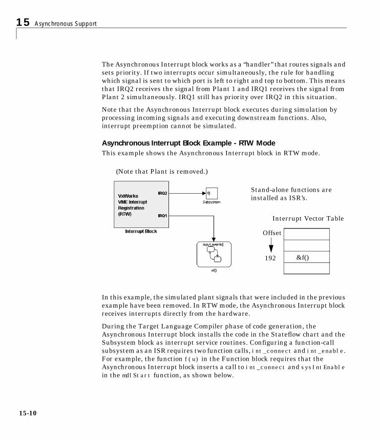
15 Asynchronous Support
15-10
The Asynchronous Interrupt block works as a “handler” that routes signals andsets priority. If two interrupts occur simultaneously, the rule for handlingwhich signal is sent to which port is left to right and top to bottom. This meansthat IRQ2 receives the signal from Plant 1 and IRQ1 receives the signal fromPlant 2 simultaneously. IRQ1 still has priority over IRQ2 in this situation.
Note that the Asynchronous Interrupt block executes during simulation byprocessing incoming signals and executing downstream functions. Also,interrupt preemption cannot be simulated.
Asynchronous Interrupt Block Example - RTW ModeThis example shows the Asynchronous Interrupt block in RTW mode.
In this example, the simulated plant signals that were included in the previousexample have been removed. In RTW mode, the Asynchronous Interrupt blockreceives interrupts directly from the hardware.
During the Target Language Compiler phase of code generation, theAsynchronous Interrupt block installs the code in the Stateflow chart and theSubsystem block as interrupt service routines. Configuring a function-callsubsystem as an ISR requires two function calls, int_connect and int_enable.For example, the function f(u) in the Function block requires that theAsynchronous Interrupt block inserts a call to int_connect and sysIntEnablein the mdlStart function, as shown below.
(Note that Plant is removed.)
Offset
192
Interrupt Vector Table
&f()
Stand-alone functions areinstalled as ISR’s.
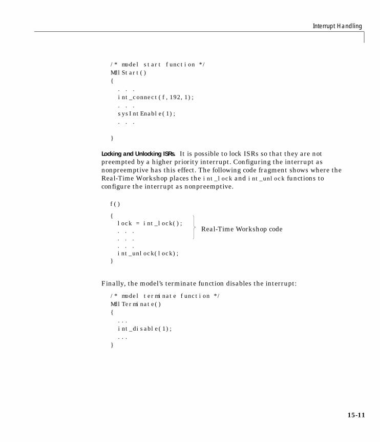
Interrupt Handling
15-11
/* model start function */MdlStart(){
. . .int_connect(f,192,1);. . .sysIntEnable(1);. . .
}
Locking and Unlocking ISRs. It is possible to lock ISRs so that they are notpreempted by a higher priority interrupt. Configuring the interrupt asnonpreemptive has this effect. The following code fragment shows where theReal-Time Workshop places the int_lock and int_unlock functions toconfigure the interrupt as nonpreemptive.
Finally, the model’s terminate function disables the interrupt:
/* model terminate function */MdlTerminate() {
...int_disable(1);...
}
Real-Time Workshop code
f()
{lock = int_lock();. . .. . .. . .int_unlock(lock);
}
15 Asynchronous Support
15-12
Task Synchronization BlockThe VxWorks Task Synchronization block is a function-call subsystem thatspawns, as an independent VxWorks task, the function-call subsystemconnected to its output. Typically it would be placed between the VxWorksAsynchronous Interrupt block and a function-call subsystem block or aStateflow chart. Another example would be to place the Task Synchronizationblock at the output of a Stateflow diagram that has an Event, “Output toSimulink,” configured as a function-call.
The VxWorks Task Synchronization block performs the following functions:
• The downstream function-call subsystem is spawned as an independent taskusing the VxWorks system call taskSpawn(). The task is deleted usingtaskDelete() during model termination.
• A semaphore is created to synchronize the downstream system to theexecution of the Task Synchronization block.
• Code is added to this spawned function-call subsystem to wrap it in aninfinite while loop.
• Code is added to the top of the infinite while loop of the spawned task to waiton a the semaphore, using semTake(). When semTake() is first called,NO_WAIT is specified. This allows the task to determine if a second semGive()has occurred prior to the completion of the function-call subsystem. Thiswould indicate the interrupt rate is too fast or the task priority is too low.
• Synchronization code, i.e., semgive(), is generated for the TaskSynchronization block (a masked function-call subsystem). This allows theoutput function-call subsystem to run. As an example, if you connect theTask Synchronization block to the output of a VxWorks AsynchronousInterrupt block, only a semGive() would occur inside an ISR.
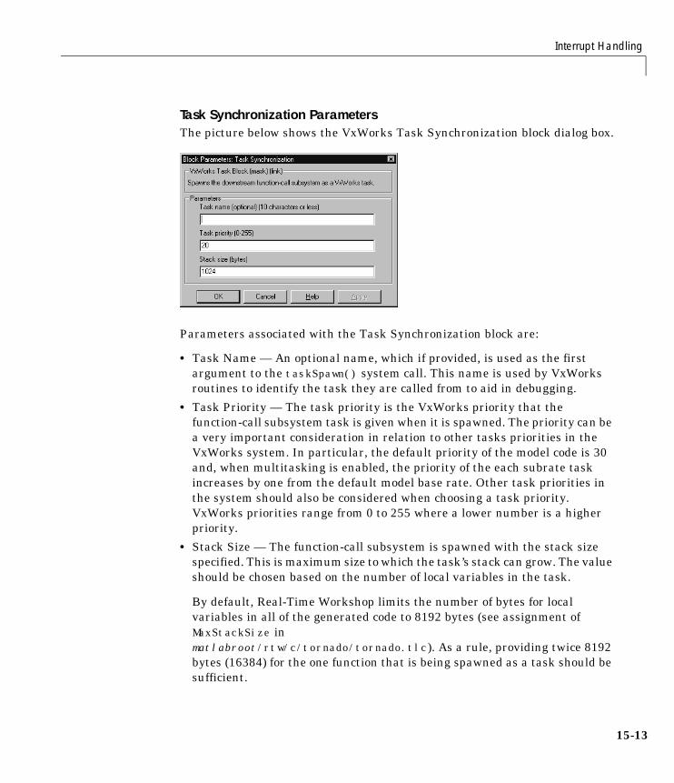
Interrupt Handling
15-13
Task Synchronization ParametersThe picture below shows the VxWorks Task Synchronization block dialog box.
Parameters associated with the Task Synchronization block are:
• Task Name — An optional name, which if provided, is used as the firstargument to the taskSpawn() system call. This name is used by VxWorksroutines to identify the task they are called from to aid in debugging.
• Task Priority — The task priority is the VxWorks priority that thefunction-call subsystem task is given when it is spawned. The priority can bea very important consideration in relation to other tasks priorities in theVxWorks system. In particular, the default priority of the model code is 30and, when multitasking is enabled, the priority of the each subrate taskincreases by one from the default model base rate. Other task priorities inthe system should also be considered when choosing a task priority.VxWorks priorities range from 0 to 255 where a lower number is a higherpriority.
• Stack Size — The function-call subsystem is spawned with the stack sizespecified. This is maximum size to which the task’s stack can grow. The valueshould be chosen based on the number of local variables in the task.
By default, Real-Time Workshop limits the number of bytes for localvariables in all of the generated code to 8192 bytes (see assignment ofMaxStackSize inmatlabroot/rtw/c/tornado/tornado.tlc). As a rule, providing twice 8192bytes (16384) for the one function that is being spawned as a task should besufficient.
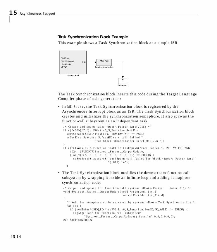
15 Asynchronous Support
15-14
Task Synchronization Block ExampleThis example shows a Task Synchronization block as a simple ISR.
The Task Synchronization block inserts this code during the Target LanguageCompiler phase of code generation:
• In MdlStart, the Task Synchronization block is registered by theAsynchronous Interrupt block as an ISR. The Task Synchronization blockcreates and initializes the synchronization semaphore. It also spawns thefunction-call subsystem as an independent task./* Create and spawn task: <Root>/Faster Rate(.015) */if ((*(SEM_ID *)rtPWork.s6_S_Function.SemID =semBCreate(SEM_Q_PRIORITY, SEM_EMPTY)) == NULL) ssSetErrorStatus(rtS,"semBCreate call failed "
"for block <Root>/Faster Rate(.015).\n ");}if ((rtIWork.s6_S_Function.TaskID = taskSpawn("root_Faster_", 20, VX_FP_TASK,
1024, (FUNCPTR)Sys_root_Faster__OutputUpdate,(int_T)rtS, 0, 0, 0, 0, 0, 0, 0, 0, 0)) == ERROR) {
ssSetErrorStatus(rtS,"taskSpawn call failed for block <Root>/ Faster Rate " "(.015).\n");
}
• The Task Synchronization block modifies the downstream function-callsubsystem by wrapping it inside an infinite loop and adding semaphoresynchronization code./* Output and update for function-call system: <Root>/Faster Rate(.015) */void Sys_root_Faster__OutputUpdate(void *reserved, int_T
controlPortIdx, int_T tid){ /* Wait for semaphore to be released by system: <Root>/Task Synchronization */ for(;;) { if (semTake(*(SEM_ID *)rtPWork.s6_S_Function.SemID,NO_WAIT) != ERROR) { logMsg("Rate for function-call subsystem" "Sys_root_Faster__OutputUpdate() fast.\n",0,0,0,0,0,0);
#if STOPONOVERRUN
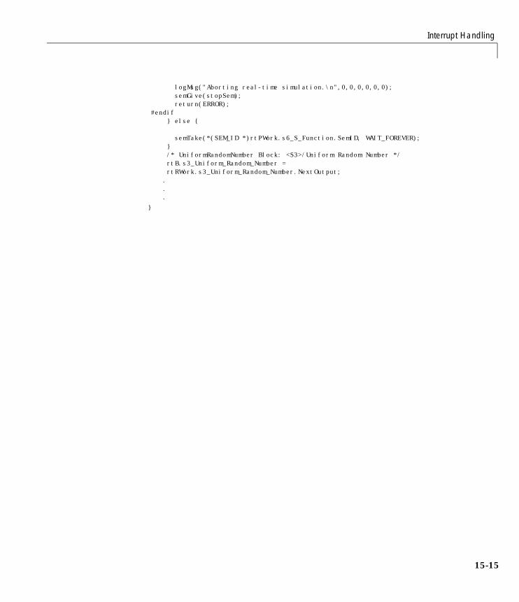
Interrupt Handling
15-15
logMsg("Aborting real-time simulation.\n",0,0,0,0,0,0); semGive(stopSem); return(ERROR);#endif } else {
semTake(*(SEM_ID *)rtPWork.s6_S_Function.SemID, WAIT_FOREVER); } /* UniformRandomNumber Block: <S3>/Uniform Random Number */ rtB.s3_Uniform_Random_Number =
rtRWork.s3_Uniform_Random_Number.NextOutput; . . .
}

15 Asynchronous Support
15-16
Asynchronous Buffer BlockThe VxWorks Asynchronous Buffer blocks are meant to be used to interfacesignals to asynchronous function-call subsystems in a model. This is neededwhenever a function-call subsystem has input or output signals and its controlinput ultimately connects (sources) to the VxWorks Asynchronous Interruptblock or Task Synchronization block.
Because an asynchronous function-call subsystem can preempt or bepreempted by other model code, an inconsistency arises when more than onesignal element is connected to it. The issue is that signals passed to and/or fromthe function-call subsystem can be in the process of being written or read whenthe preemption occurs. Thus, partial old and partial new data will be used.
This situation can also occur with scalar signals in some cases. For example, ifa signal is a double (8 bytes), the read or write operation may require twoassembly instructions.
The Asynchronous Buffer blocks can be used to guarantee the data passed toand/or from the function-call subsystem is all from the same iteration.
The Asynchronous Buffer blocks are used in pairs, with a write side driving theread side. To ensure the data integrity, no other connections are allowedbetween the two Asynchronous Buffer blocks. The pair works by using twobuffers (“double buffering”) to pass the signal and, by using mutually exclusivecontrol, allow only exclusive access to each buffer. For example, if the write sideis currently writing into one buffer, the read side can only read from the otherbuffer.
The initial buffer is filled with zeros so that if the read side executes before thewrite side has had time to fill the other buffer, the read side will collect zerosfrom the initial buffer.
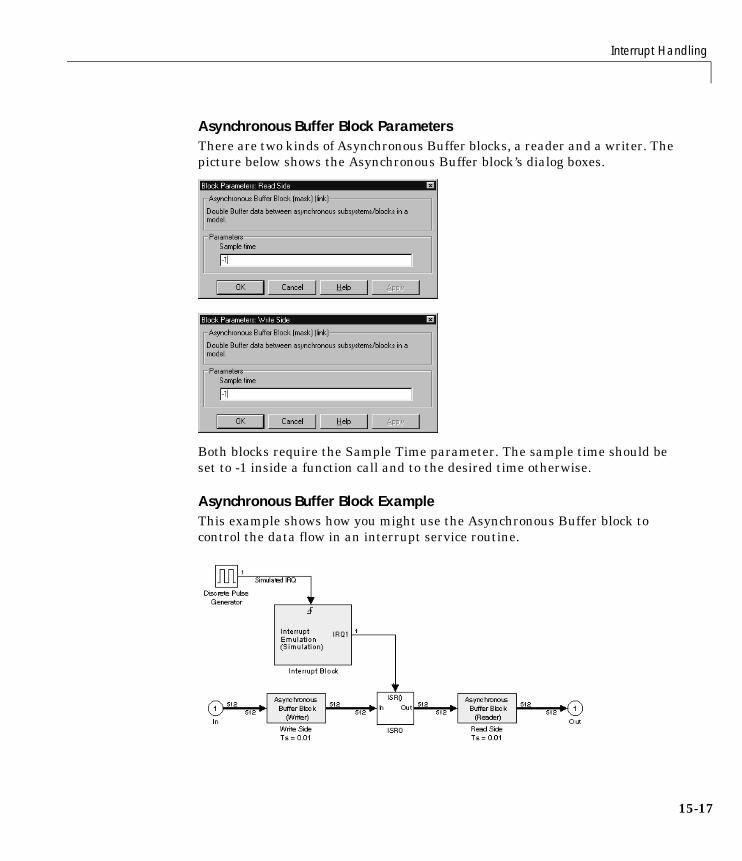
Interrupt Handling
15-17
Asynchronous Buffer Block ParametersThere are two kinds of Asynchronous Buffer blocks, a reader and a writer. Thepicture below shows the Asynchronous Buffer block’s dialog boxes.
Both blocks require the Sample Time parameter. The sample time should beset to -1 inside a function call and to the desired time otherwise.
Asynchronous Buffer Block ExampleThis example shows how you might use the Asynchronous Buffer block tocontrol the data flow in an interrupt service routine.
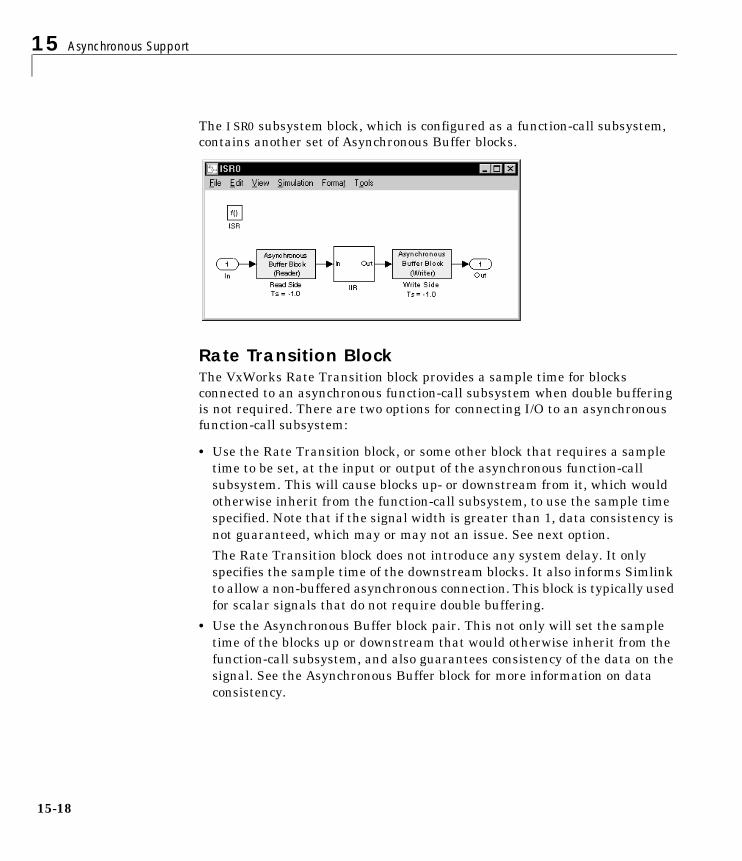
15 Asynchronous Support
15-18
The ISR0 subsystem block, which is configured as a function-call subsystem,contains another set of Asynchronous Buffer blocks.
Rate Transition BlockThe VxWorks Rate Transition block provides a sample time for blocksconnected to an asynchronous function-call subsystem when double bufferingis not required. There are two options for connecting I/O to an asynchronousfunction-call subsystem:
• Use the Rate Transition block, or some other block that requires a sampletime to be set, at the input or output of the asynchronous function-callsubsystem. This will cause blocks up- or downstream from it, which wouldotherwise inherit from the function-call subsystem, to use the sample timespecified. Note that if the signal width is greater than 1, data consistency isnot guaranteed, which may or may not an issue. See next option.
The Rate Transition block does not introduce any system delay. It onlyspecifies the sample time of the downstream blocks. It also informs Simlinkto allow a non-buffered asynchronous connection. This block is typically usedfor scalar signals that do not require double buffering.
• Use the Asynchronous Buffer block pair. This not only will set the sampletime of the blocks up or downstream that would otherwise inherit from thefunction-call subsystem, and also guarantees consistency of the data on thesignal. See the Asynchronous Buffer block for more information on dataconsistency.

Interrupt Handling
15-19
Rate Transition Block ParametersThis picture shows the VxWorks Rate Transition block’s dialog box.
The Sample time parameter sets the sample time to the desired rate.
Rate Transition Block ExampleThis picture shows a sample application of the Rate Transition block in an ISR.
In this example, the Rate Transition block on the input to the function-callsubsystem causes both the In and Gain1 blocks to run at the 0.1 second rate.The Rate Transition block on the output of the function-call subsystem causesboth the Gain2 and Out blocks to run at the 0.2 second rate. Using this schemeinforms Simlink to allow non-buffered connections to an asynchronousfunction-call subsystem.

15 Asynchronous Support
15-20
Creating a Customized Asynchronous LibraryYou can use the Real-Time Workshop’s VxWorks asynchronous blocks astemplates that provide a starting point for creating your own asynchronousblocks. Templates are provided for these blocks:
• Asynchronous Buffer block
• Asynchronous Interrupt block
• Rate Transition block
• Task Synchronization block
You can customize each of these blocks by implementing a set of modificationsto files associated with each template. These files are:
• The block’s underlying S-function C MEX-file
• The block’s mask and the associated mask M-file
• The TLC files that control code generation of the block
At a minimum, you must rename the system calls generated by the TLC filesto the correct names for the new real-time operating system (RTOS) and supplythe correct arguments for each file. There is a collection of files that you mustcopy (and rename) from matlabroot/rtw/c/tornado/devices into a newdirectory, for example, matlabroot/rtw/c/my_os/devices. These files are:
• Asynchronous Buffer block — vxdbuffer.tlc, vxdbuffer.c
• Asynchronous Interrupt block — vxinterrupt.tlc, vxinterrupt.c,vxintbuild.m
• O/S include file — vxlib.tlc
• Task Synchronization block — vxtask.tlc, vxtask.c
16Real-Time Workshop AdaCoder
Introduction . . . . . . . . . . . . . . . . . . . . 16-2
Getting Started . . . . . . . . . . . . . . . . . . . 16-6
Configuring and Interfacing Parameters and Signals . 16-16
Code Validation . . . . . . . . . . . . . . . . . . 16-18
Supported Blocks . . . . . . . . . . . . . . . . . 16-21
16 Real-Time Workshop Ada Coder
16-2
IntroductionThis chapter presents an introduction to the Real-Time Workshop Ada Coder.It compares and contrasts the Real-Time Workshop Ada Coder with theReal-Time Workshop, shows you how to use the product by presenting anexample, and concludes with a discussion of code validation.
Note The Real-Time Workshop Ada Coder is a separate product from theReal-Time Workshop.
Like the Real-Time Workshop, the Real-Time Workshop Ada Coder provides areal-time development environment that features:
• A rapid and direct path from system design to hardware implementation
• Seamless integration with MATLAB and Simulink
• A simple, easy-to-use interface
• An open and extensible architecture
The package includes application modules that allow you to build completeprograms targeting a wide variety of environments. Program building is fullyautomated. Automatic program building provides a standard means to createprograms for real-time applications. This chapter contains examples ofautomatic program building on DOS and UNIX platforms.
The Real-Time Workshop Ada Coder is an automatic Ada language codegenerator. It produces Ada83 or Ada95 code directly from Simulink models andautomatically builds programs that can be run in real time in a variety ofenvironments. The Real-Time Workshop Ada Coder is an extension of theReal-Time Workshop.
With the Real-Time Workshop Ada Coder, you can run your Simulink model inreal time on a remote processor. You can run accelerated, stand-alonesimulations on your host machine or on an external computer.
16-3
Real-Time Workshop Ada Coder ApplicationsLike the Real-Time Workshop, the Real-Time Workshop Ada Coder supports avariety of real-time applications:
• Real-Time Control — You can design your control system using MATLABand Simulink and generate Ada code from your block diagram model. Youcan then compile and download the Ada code directly to your targethardware.
• Hardware-in-the-Loop Simulation — You can use Simulink to model real-lifemeasurement and actuation signals. You can use the code generated fromthe model on special-purpose hardware to provide a real-time representationof the physical system. Applications include control system validation,training simulation, and fatigue testing using simulated load variations.
Supported CompilersThe generated code will work with any validated Ada83 or Ada95 compiler.Real-Time Workshop provides an example target that uses the GNAT Ada95compiler. You can download a free version of this compiler from the GNAT ftpsite (ftp://cs.nyu.edu/pub/gnat). You can also purchase a professionalversion from Ada Core Technologies (www.gnat.com).
Supported TargetsThe Real-Time Workshop Ada Coder supports the following targets:
• Ada Simulation Target — Useful for validating generated code. This does notuse Ada tasking primitives.
• Ada Multitasking Real-Time Target — Useful as a starting point fortargeting real-time systems. This uses Ada tasking primitives.
• Ada83 target — The generated Ada83 code does not support data logging,but is suitable for generating embedded code for use with legacy Ada83compilers. The Ada83 target is available from the System Target FileBrowser by selecting the system target file rt_ada83.tlc (Ada83 Target forGNAT). The accompanying template makefile gnat83.tmf uses the -gnat83switch in the GNAT Ada95 compiler.
16 Real-Time Workshop Ada Coder
16-4
You can also add your own target by creating a system target file, makeprocess, and run-time interface files along with any device drivers usinginlined Ada or C S-functions.
The Generated CodeThe generated code (i.e., the model code) is highly optimized, fully commented,and can be generated from any discrete-time Simulink model — linear ornonlinear.
All Simulink blocks are automatically converted to code, with the exception of:
• MATLAB function blocks
• Any continuous sample time blocks
• S-functions that are not inlined using the Target Language Compiler
Types of OutputThe Real-Time Workshop Ada Coder’s interface supports two forms of output:
• Ada code − Generate code that contains system equations and initializationfunctions for the Simulink model. You can use this code in real-timeapplications.
• A real-time program − Transform the generated code into a real-timeprogram suitable for use with dedicated real-time hardware. The resultingcode is designed to interface with an external clock source and hence runs ata fixed, user-specified sample rate.
Supported BlocksSee “Supported Blocks” on page 16–21 for a complete list of the Simulink blockssupported by the Real-Time Workshop Ada Coder.
RestrictionsThe Real-Time Workshop Ada Coder has the same constraints imposed upon itas the Real-Time Workshop Embedded Coder target. The code generator doesnot produce code that solves algebraic loops, and Simulink blocks that aredependent on absolute time can be used only if the program is not intended torun for an indefinite period of time.
16-5
There are additional constraints for the Ada code generation. The Real-TimeWorkshop Ada Coder does not provide:
• Nonreal-time variable step integration models
• Continuous-time integration
• Since Ada does not support implicit upcasting of data types, all numericaloperations in your model must be of homogeneous data types for Ada codegeneration. You can, however, perform explicit upcasting using the DataType Conversion block in Simulink.
• You must inline all Ada S-functions with a corresponding TLC file (see theTarget Language Compiler Reference Guide for more information aboutinlining S-functions)
• External mode is not supported with the Real-Time Workshop Ada Coder.

16 Real-Time Workshop Ada Coder
16-6
Getting Started This section illustrates, through a simple example, how to transform aSimulink model into a stand-alone executable program. This program runsindependently of Simulink, allowing accelerated execution on the developmenthost or a different target computer.
Generating Ada code from a Simulink model is very similar to generating Ccode. Begin by typing
countersdemo
at the MATLAB prompt. This block diagram appears.
Figure 16-1: Counter Demonstration with Subsystems Open
Getting Started
16-7
Setting Options for Ada Code GenerationYou must specify the correct options before you generate Ada code from thismodel. These are the steps:
1 Select Parameters under the Simulation menu. This opens the SimulationParameters dialog box.
2 On the Solver page, set the Solver options to Fixed-step discrete (nocontinuous states)
3 Select the Real-Time Workshop page. In the Category menu, select Targetconfiguration.
4 Click the Browse button. This opens the System Target File Browser.

16 Real-Time Workshop Ada Coder
16-8
5 Select Ada Simulation Target for GNAT and click OK. This automaticallysets the correct System target file, Template makefile, and Makecommand fields for Ada code generation.
Figure 16-2 shows the System Target File Browser with the correct selectionfor Ada code generation.
Figure 16-2: The System Target File Browser
Alternatively, you can specify the settings on the Real-Time Workshop pagemanually by following these steps:
1 Select Options under the Real-Time Workshop submenu of the Toolsmenu. This opens the Real-Time Workshop page of the SimulationParameters dialog box.
2 In the Category menu, select Target configuration.
3 Specify rt_ada_sim.tlc as the System target file.
4 Specify gnat_sim.tmf as the Template makefile.
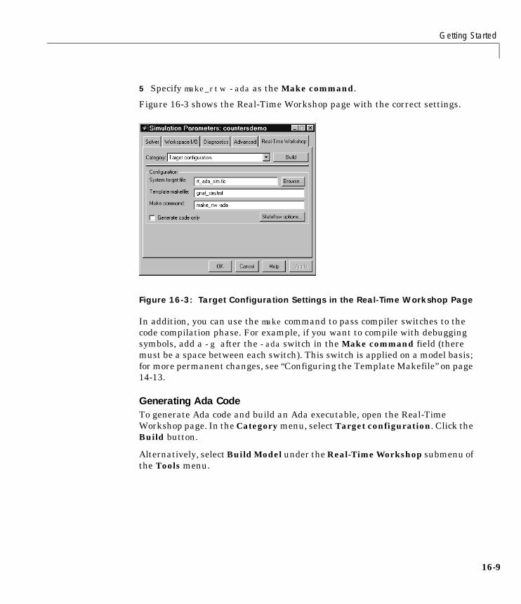
Getting Started
16-9
5 Specify make_rtw -ada as the Make command.
Figure 16-3 shows the Real-Time Workshop page with the correct settings.
Figure 16-3: Target Configuration Settings in the Real-Time Workshop Page
In addition, you can use the make command to pass compiler switches to thecode compilation phase. For example, if you want to compile with debuggingsymbols, add a -g after the -ada switch in the Make command field (theremust be a space between each switch). This switch is applied on a model basis;for more permanent changes, see “Configuring the Template Makefile” on page14-13.
Generating Ada CodeTo generate Ada code and build an Ada executable, open the Real-TimeWorkshop page. In the Category menu, select Target configuration. Click theBuild button.
Alternatively, select Build Model under the Real-Time Workshop submenu ofthe Tools menu.
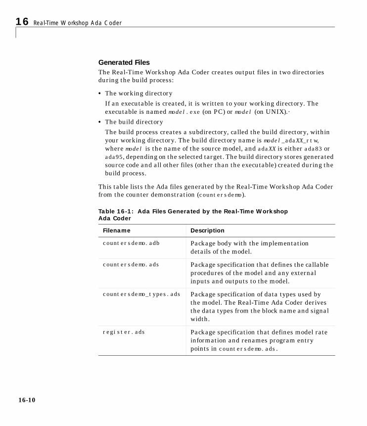
16 Real-Time Workshop Ada Coder
16-10
Generated FilesThe Real-Time Workshop Ada Coder creates output files in two directoriesduring the build process:
• The working directory
If an executable is created, it is written to your working directory. Theexecutable is named model.exe (on PC) or model (on UNIX).·
• The build directory
The build process creates a subdirectory, called the build directory, withinyour working directory. The build directory name is model_adaXX_rtw,where model is the name of the source model, and adaXX is either ada83 orada95, depending on the selected target. The build directory stores generatedsource code and all other files (other than the executable) created during thebuild process.
This table lists the Ada files generated by the Real-Time Workshop Ada Coderfrom the counter demonstration (countersdemo).
Table 16-1: Ada Files Generated by the Real-Time Workshop Ada Coder
Filename Description
countersdemo.adb Package body with the implementationdetails of the model.
countersdemo.ads Package specification that defines the callableprocedures of the model and any externalinputs and outputs to the model.
countersdemo_types.ads Package specification of data types used bythe model. The Real-Time Ada Coder derivesthe data types from the block name and signalwidth.
register.ads Package specification that defines model rateinformation and renames program entrypoints in countersdemo.ads.
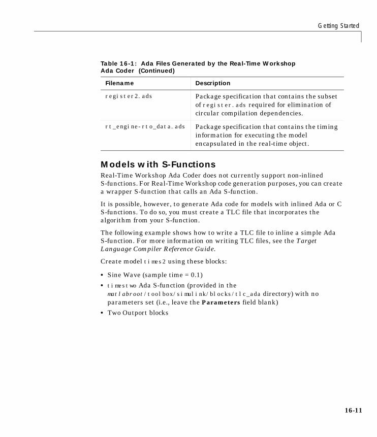
Getting Started
16-11
Models with S-FunctionsReal-Time Workshop Ada Coder does not currently support non-inlinedS-functions. For Real-Time Workshop code generation purposes, you can createa wrapper S-function that calls an Ada S-function.
It is possible, however, to generate Ada code for models with inlined Ada or CS-functions. To do so, you must create a TLC file that incorporates thealgorithm from your S-function.
The following example shows how to write a TLC file to inline a simple AdaS-function. For more information on writing TLC files, see the TargetLanguage Compiler Reference Guide.
Create model times2 using these blocks:
• Sine Wave (sample time = 0.1)
• timestwo Ada S-function (provided in thematlabroot/toolbox/simulink/blocks/tlc_ada directory) with noparameters set (i.e., leave the Parameters field blank)
• Two Outport blocks
register2.ads Package specification that contains the subsetof register.ads required for elimination ofcircular compilation dependencies.
rt_engine-rto_data.ads Package specification that contains the timinginformation for executing the modelencapsulated in the real-time object.
Table 16-1: Ada Files Generated by the Real-Time Workshop Ada Coder (Continued)
Filename Description
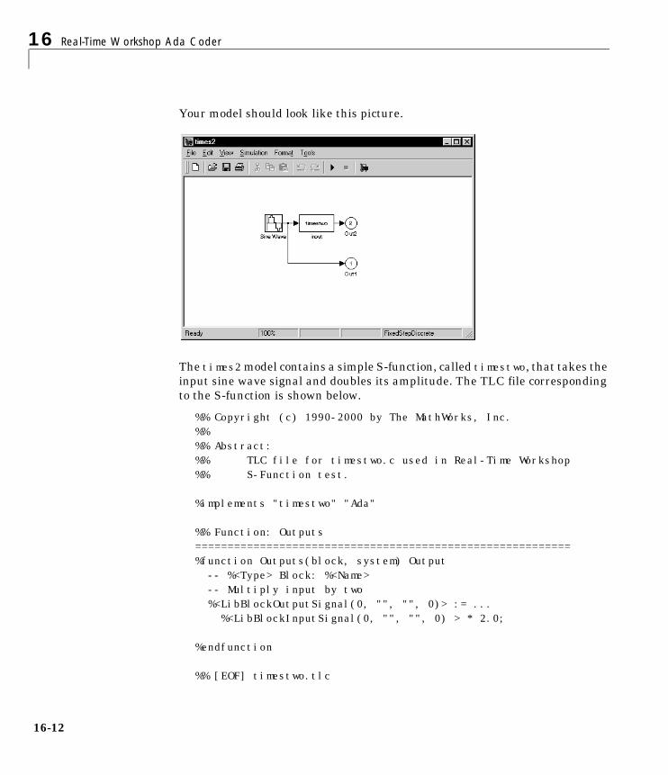
16 Real-Time Workshop Ada Coder
16-12
Your model should look like this picture.
The times2model contains a simple S-function, called timestwo, that takes theinput sine wave signal and doubles its amplitude. The TLC file correspondingto the S-function is shown below.
%% Copyright (c) 1990-2000 by The MathWorks, Inc.%%%% Abstract:%% TLC file for timestwo.c used in Real-Time Workshop %% S-Function test.
%implements "timestwo" "Ada" %% Function: Outputs ==========================================================%function Outputs(block, system) Output -- %<Type> Block: %<Name> -- Multiply input by two %<LibBlockOutputSignal(0, "", "", 0)> := ...
%<LibBlockInputSignal(0, "", "", 0) > * 2.0;
%endfunction
%% [EOF] timestwo.tlc

Getting Started
16-13
The key line in this TLC file is the assignment of two times theLibBlockInputSignal to the LibBlockOutputSignal. This line directs theTarget Language Compiler to place the algorithm directly into the generatedAda code.
This TLC file is located inmatlabroot/toolbox/simulink/blocks/tlc_ada/timestwo.tlc.
Generating the Ada CodeThe build process is similar to the case where your model does not contain anyS-functions. The only additional requirement for generating Ada code formodels containing S-functions is to provide a TLC file with the same name asthe S-function. Otherwise, the build procedure is exactly the same.
Configuring the Template MakefileTemplate makefiles specify the compiler, link, and make directives native tothe target computer’s operating system and compiler you are using. Twoexamples of template makefiles are provided in the directorymatlab/rtw/ada/gnat. File gnat_sim.tmf is the template makefile that buildsthat real-time Ada simulation program. The automatic build process expandsthe macros defined at the top of the .tmf file to create the call to gnatmake.gnatmake then compiles and links the program.
There are two ways to make permanent changes to the template makefile if youneed to make modifications either to target a different Ada95 compiler or tomake minor adjustments to the gnat make directive:
• Copy the template makefile into the directory where the model is located.
• Copy the template makefile to a unique name in matlab/rtw/ada/gnat andmake modifications to the new file.
Data LoggingYou can use the Ada real-time simulation target (rt_ada_sim) to perform thesame data logging as a Simulink simulation. To enable MAT-file logging, selectAda-specific code generation options item in the Category menu of theReal-Time Workshop page. Then select the MAT-file logging option. Whenthis option is selected, the Ada program executes for the duration specified bythe Stop time field on the Solver page of the Simulation Parameters dialogbox.
16 Real-Time Workshop Ada Coder
16-14
When the Ada Coder finishes its run, a model.mat file is created that containsall workspace variables that would have been created by running a Simulinksimulation. The names of these workspace variables are the same as the namesthat would have been created by Simulink, except that an rt_ prefix isattached. See “Workspace I/O Options and Data Logging” in Chapter 3 for moreinformation about data logging.
Note If you do not select MAT-file logging, the stop time is ignored and theAda program runs without stopping.
Generating Block CommentsWhen the Insert block descriptions in code option is selected, comments areinserted into the code generated for any blocks that have text in theirDescription fields. To generate block comments:
1 Right-click on the block you want to comment. Select Block Properties fromthe context menu. The Block Properties dialog box opens.
2 Type the comment into the Description field.
3 Select the Insert block descriptions in code option in the Ada-specific codegeneration options category of the Real-Time Workshop page.
Note For virtual blocks or blocks that have been removed due to blockreduction optimizations, no comments are generated.
Application Modules Required for the Real-Time ProgramBuilding the real-time program requires a number of support files in additionto the generated code. These support files contain:
• A main program
• Code to drive execution of the model code
• Code to carry out data logging
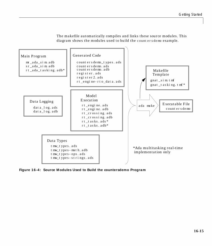
Getting Started
16-15
The makefile automatically compiles and links these source modules. Thisdiagram shows the modules used to build the countersdemo example.
Figure 16-4: Source Modules Used to Build the countersdemo Program
Generated Code
countersdemo.adsmr_ada_sim.adb
Main Program
rt_engine.ads
Model
Data Typestmw_types.adstmw_types-math.adb
Executable Filecountersdemo
ExecutionData Logging
data_log.ads
MakefileTemplate
gnat_sim.tmf
ada make
countersdemo_types.ads
countersdemo.adbregister.ads
sr_ada_sim.adb
rt_engine.adbdata_log.adb
tmw_types-ops.adstmw_types-strings.ads
gnat_tasking.tmf*
register2.ads
rt_crossing.adsrt_crossing.adb
rt_ada_tasking.adb*
rt_tasks.ads*rt_tasks.adb*
*Ada multitasking real-timeimplementation only
rt_engine-rto_data.ads
16 Real-Time Workshop Ada Coder
16-16
Configuring and Interfacing Parameters and Signals
Model Parameter ConfigurationThe Model Parameter Configuration dialog provides a mechanism forinterfacing your model’s block parameters to code that you have written. Thisis useful in situations where you want your hand-written code to changeparameter values while the generated program executes.
Read “Parameters: Storage, Interfacing, and Tuning” on page 3-51 to learnabout general parameter storage concepts and the Model ParameterConfiguration dialog.
Using the Model Parameter Configuration dialog does not differ greatlybetween between Ada and other target languages such as C. However, youshould note the following Ada-specific differences:
• The Storage Type Qualifier field is only used when specifying the packagespecification to fully qualify the variable name for the ImportedExternoption. This field is ignored in all other cases.
• ImportedExtern variables are assumed to be declared in the packagespecification entered in the Storage Type Qualifier field. The generatedcode accesses this variable as Your_Package.Your_variable.
• ImportedExternPointer storage class is not permitted in Ada.
Signal PropertiesThe Simulink Signal Properties dialog lets you interface selected signals toexternally written code. In this way, your hand-written code has access to suchsignals for monitoring or other purposes.
Read “Signals: Storage, Optimization, and Interfacing” on page 3-65 to learnabout general signal storage concepts and the Signal Properties dialog. Thennote the Ada-specific differences described below.
The Real-Time Workshop Ada Coder has logic for supporting Simulink signallabels. This logic automatically maps signal labels to Simulink blocks based onthe block name, signal name, and connectivity. You can override the defaultbehavior and either specify an external declaration for the signal name ordirect the Real-Time Workshop Ada Coder to declare a unique declaration ofthe signal that is visible in the generated model package specification. The
Configuring and Interfacing Parameters and Signals
16-17
heuristics are implemented on a signal basis as specified by the Signal name,RTW storage class, and RTW storage type qualifier (externally declaredsignals only).
The options relevant to the Real-Time Workshop Ada Coder are:
• SimulinkGlobal (Test Point): Clicking this check box directs the Real-TimeWorkshop Ada Coder to place the signal in a unique global memory location(rtB structure). This is useful for testing purposes since it eliminates thepossibility of overwriting the signal data. Note that selecting this optionforces the RTW storage class to be Auto.
• RTW storage class : The storage class options are:
- Auto: directs the Real-Time Workshop to store the signal in a persistentdata structure. Specifically, an element called Signal_Name is declared inthe External_Inputs structure defined in the Model_Types packagespecification. The generated code accesses this signal asRT_U.Signal_Name.
- ExportedGlobal: Declares the signal as a global variable that can beaccessed from outside the generated code. The signal is declared in themodel package specification but not in the External_Inputs structure.The generated code accesses this signal as Signal_Name. The signal will beglobally visible as Model.Signal_Name.
- ImportedExtern: The signal is assumed to be declared in the packagespecification entered in the RTW storage type qualifier field. Thegenerated code accesses this signal as Your_Package.Signal_Name.
- ImportedExternPointer: This is not permitted in Ada.
• RTW storage type qualifier : This is only used when specifying the packagespecification to qualify fully the signal name for the Imported Extern option.This field is ignored in all other cases.
These cases are useful if you want to link Real-Time Workshop Ada Codergenerated code to other Ada code (i.e., code that the Real-Time Workshop AdaCoder did not generate).
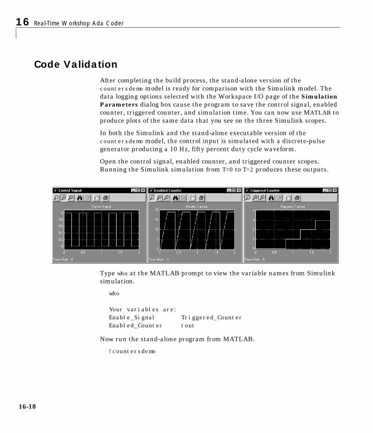
16 Real-Time Workshop Ada Coder
16-18
Code ValidationAfter completing the build process, the stand-alone version of thecountersdemo model is ready for comparison with the Simulink model. Thedata logging options selected with the Workspace I/O page of the SimulationParameters dialog box cause the program to save the control signal, enabledcounter, triggered counter, and simulation time. You can now use MATLAB toproduce plots of the same data that you see on the three Simulink scopes.
In both the Simulink and the stand-alone executable version of thecountersdemo model, the control input is simulated with a discrete-pulsegenerator producing a 10 Hz, fifty percent duty cycle waveform.
Open the control signal, enabled counter, and triggered counter scopes.Running the Simulink simulation from T=0 to T=2 produces these outputs.
Type who at the MATLAB prompt to view the variable names from Simulinksimulation.
who
Your variables are:Enable_Signal Triggered_Counter Enabled_Counter tout
Now run the stand-alone program from MATLAB.
!countersdemo
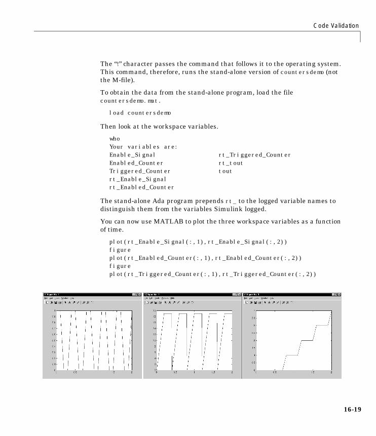
Code Validation
16-19
The “!” character passes the command that follows it to the operating system.This command, therefore, runs the stand-alone version of countersdemo (notthe M-file).
To obtain the data from the stand-alone program, load the filecountersdemo.mat.
load countersdemo
Then look at the workspace variables.
whoYour variables are:Enable_Signal rt_Triggered_Counter Enabled_Counter rt_tout Triggered_Counter tout rt_Enable_Signal rt_Enabled_Counter
The stand-alone Ada program prepends rt_ to the logged variable names todistinguish them from the variables Simulink logged.
You can now use MATLAB to plot the three workspace variables as a functionof time.
plot(rt_Enable_Signal(:,1),rt_Enable_Signal(:,2))figureplot(rt_Enabled_Counter(:,1),rt_Enabled_Counter(:,2))figureplot(rt_Triggered_Counter(:,1),rt_Triggered_Counter(:,2))
16 Real-Time Workshop Ada Coder
16-20
Analyzing Data with MATLABPoints to consider when data logging:
• Ada95 code supports all data logging formats (matrix, structure, andstructure/time).
• Ada83 code does not support data logging.
• To Workspace blocks log data at the frequency of the driving block and do notlog time.
• Scope blocks log data at the frequency of the driving block and log time in thefirst column of the matrix.
• Root Outport blocks are updated at the frequency of the driving block but arelogged at the base rate of the model.

Supported Blocks
16-21
Supported BlocksThe Real-Time Workshop Ada Coder supports the following Simulink blocks.
Discrete Blocks
Discrete-Time Integrator Discrete Zero-Pole
Discrete Filter Unit Delay
Discrete State-Space Zero-Order Hold
Discrete Transfer Fcn
Functions & Tables
Direct Look-Up Table (n-D) Look-Up Table (2-D)
Fcn Look-Up Table (n-D)
Interpolation (n-D) UsingPreLook-Up Index Search
PreLook-Up Index Search
Look-Up Table S-Function — Only TargetLanguage Compiler inlinedS-functions are supported
Math Blocks
Abs MinMax
Bitwise Logical Operator Product — matrix multiplicationand element-wise multiplicationand division are supported. Matrixdivision is not supported.
Combinatorial Logic Real-Imag to Complex
Complex to Magnitude-Angle Relational Operator
Complex to Real-Imag Rounding Function
16 Real-Time Workshop Ada Coder
16-22
Dot Product Sign
Gain (inluding matrix/element-wise)
Slider Gain
Logic Operator Sum
Magnitude-Angle to Complex Trigonometric Function
Math Function
Nonlinear Blocks
Backlash Quantizer
Coulomb & Viscous Friction Relay
DeadZone Saturation
Manual Switch (must BreakLibrary Link and use discretesample time)
Switch
Multiport Switch
Signals & Systems Blocks
Bus Selector Initial Condition (IC)
Configurable Subsystem Inport
DataStore Memory Matrix Concatenation
DataStore Read Merge
DataStore Write ModelInfo
Data Type Conversion Outport
Demux Probe
Math Blocks (Continued)

Supported Blocks
16-23
Enable Reshape
From Selector
Goto Tag Visibility Subsystem
Goto Terminator
Ground Trigger Width
Hit Crossing
Sinks
Display — no code is generated forthis block
To File
Scope To Workspace
Stop Simulation
Sources
Band-Limited White Noise Ramp — You must break thelibrary link and replace the clockwith a discrete clock and manuallyset the sample time step to matchthe discrete clock.
Chirp Signal — (you must breakthe library link and use a discreteclock)
Random Number
Constant Sine Wave
Signals & Systems Blocks (Continued)
16 Real-Time Workshop Ada Coder
16-24
Note All element-wise operation blocks are suported by the Real-TimeWorkshop Ada Coder.
Digital Clock Repeating Sequence — You mustbreak the library link and replacethe clock with a discrete clock andmanually set the sample time stepto match the discrete clock.
Discrete Pulse Generator Step
From File Uniform Random Number
Sources (Continued)
17Targeting Real-TimeSystems
Introduction . . . . . . . . . . . . . . . . . . . . 17-2
Components of a Custom Target Configuration . . . . . 17-4
Tutorial: Creating a Custom Target Configuration . . . . 17-9
Customizing the Build Process . . . . . . . . . . . 17-16
Creating Device Drivers . . . . . . . . . . . . . . 17-34
Interfacing Parameters and Signals . . . . . . . . . 17-65
Creating an External Mode Communication Channel . 17-73
Combining Multiple Models . . . . . . . . . . . . 17-82
DSP Processor Support . . . . . . . . . . . . . . 17-86
17 Targeting Real-Time Systems
17-2
IntroductionThe target configurations bundled with the Real-Time Workshop are suitablefor many different applications and development environments. Third-partytargets provide additional versatility. However, a number of users find thatthey require a custom target configuration.You may want to implement acustom target configuration for any of the following reasons:
• To support custom hardware and incorporate custom device driver blocksinto your models.
• To customize a bundled target configuration — such as the generic real-time(GRT) or Real-Time Workshop Embedded Coder targets — to your needs.
• To configure the build process for a special compiler (such as a compiler foran embedded microcontroller or DSP board).
As part of your custom target implementation, you may also need to:
• Interface generated model code with existing supervisory or supporting codethat calls the generated code.
• Interface signals and parameters within generated code to your own code.
• Combine code generated from multiple models into a single system.
• Implement external mode communication via your own low-level protocollayer.
The following sections provide the information necessary to accomplish thesetasks:
• “Components of a Custom Target Configuration” on page 17-4 gives anoverview of the code and control files that make up a custom targetconfiguration.
• “Tutorial: Creating a Custom Target Configuration” on page 17–9 is ahands-on exercise in building a custom rapid prototyping target.
• “Customizing the Build Process” on page 17–16 provides information on thestructure of system target files (“System Target File Structure” on page 17–16) and template makefiles (“Template Makefiles” on page 17–25).
• “Adding a Custom Target to the System Target File Browser” on page 17–24shows you how to make your custom target configuration available to usersvia the System Target File Browser.
17-3
• “Creating Device Drivers” on page 17–34 discusses the implementation ofdevice drivers as S-Function blocks, covering both inlined and noninlineddrivers.
• “Interfacing Parameters and Signals” on page 17–65 contains guidelines foruse of the Real-Time Workshop signal monitoring and parameter tuningAPIs.
• “Creating an External Mode Communication Channel” on page 17–73provides information you will need to support external mode on your customtarget, using your own low-level communications layer.
• “Combining Multiple Models” on page 17–82 discusses strategies forcombining several models (or several instances of the same model) into asingle executable.
17 Targeting Real-Time Systems
17-4
Components of a Custom Target ConfigurationThe components of a custom target configuration are:
• Code to supervise and support execution of generated model code
• Control files:
- A system target file to control the code generation process
- A template makefile to build the real-time executable
This section summarizes key concepts and terminology you will need to knowto begin developing each component. References to more detailed informationsources are provided, in case any of these topics are unfamiliar to you.
Code ComponentsA Real-Time Workshop program containing code generated from a Simulinkmodel consists of a number of code modules and data structures. These fall intotwo categories.
Application ComponentsApplication components are those which are specific to a particular model; theyimplement the functions represented by the blocks in the model. Applicationcomponents are not specific to the target. Application components include:
• Modules generated from the model
• User-written blocks (S-functions)
• Parameters of the model that are visible, and can be interfaced to, externalcode
Run-Time Interface ComponentsA number of code modules and data structures, referred to collectively as therun-time interface, are responsible for managing and supporting the executionof the generated program. The run-time interface modules are notautomatically generated. To develop a custom target, you must implement

Components of a Custom Target Configuration
17-5
certain parts of the run-time interface. Table 17-1 summarizes the run-timeinterface components.
The components of the run-time interface vary, depending upon whether thetarget is an embedded system or a rapid prototyping environment.
User-Written Run-Time Interface CodeMost of the run-time interface is provided by Real-Time Workshop. You mustimplement the following elements:
• A timer interrupt service routine (ISR). The timer runs at the program’s basesample rate. The timer ISR is responsible for operations that must becompleted within a single clock period, such as computing the current outputsample.The timer ISR usually calls the Real-Time Workshop suppliedfunction, rt_OneStep.
• The main program. Your main program initializes the blocks in the model,installs the ISR, and executes a background task or loop. The timerperiodically interrupts the main loop. If the main program is designed to runfor a finite amount of time, it is also responsible for cleanup operations - suchas memory deallocation and masking the timer interrupt - beforeterminating the program.
• Device drivers to communicate with your target hardware.
Table 17-1: Run-Time Interface Components
User Provides: Real-Time Workshop Provides:
Customized main program Generic main program
Timer interrupt handler torun model
Execution engine and integrationsolver (called by timer interrupthandler)
Other interrupt handlers Example interrupt handlers(Asynchronous Interrupt Blocks)
Device drivers Example device drivers
Data logging and signalmonitoring user interface
Data logging, parameter tuning,signal monitoring, and external modesupport
17 Targeting Real-Time Systems
17-6
Run-Time Interface for Rapid PrototypingThe run-time interface for a rapid prototyping target includes:
• Supervisory logic
- The main program
- Execution engine and integration solver
• Supporting logic
- I/O drivers
- Code to handle timing, and interrupts
• Monitoring, tuning, and debugging support
- Data logging code
- Signal monitoring
- Real-time parameter tuning
- External mode communications
The structure of the rapid prototyping run-time interface, and the execution ofrapid prototyping code, are detailed in Chapter 6, “Program Architecture” andChapter 7, “Models with Multiple Sample Rates.”
Development of a custom rapid prototyping target generally begins withcustomization of one of the generic main programs, grt_main.c orgrt_malloc_main.c. As described in “User-Written Run-Time Interface Code”above, you must modify the main program for real-time interrupt-drivenexecution. You must also supply device drivers (optionally inlined).
Run-Time Interface for Embedded TargetsThe run-time interface for an embedded (production) target includes:
• Supervisory logic
- The main program
- Execution engine and integration solver
• Supporting logic
- I/O drivers
- Code to handle timing, and interrupts

Components of a Custom Target Configuration
17-7
• Monitoring and debugging support
- Data logging code
- Access to tunable parameters and external signals
Development of a custom embedded target generally begins with customizationof the Real-Time Workshop Embedded Coder main program, ert_main.c.Chapter 9, “Real-Time Workshop Embedded Coder” details the structure of theReal-Time Workshop Embedded Coder run-time interface and the execution ofReal-Time Workshop Embedded Coder code, and provides guidelines forcustomizing ert_main.c.
Control Files
System Target FilesThe Target Language Compiler (TLC) generates target-specific C or Ada codefrom an intermediate description of your Simulink block diagram (model.rtw).The Target Language Compiler reads model.rtw and executes a programconsisting of several target files (.tlc files.) The output of this process is anumber of source files, which are fed to your development system’s makeutility.
The system target file controls the code generation process. You will need tocreate a customized system target file to set code generation parameters foryour target. We recommend that you copy, rename, and modify one of thestandard system target files:
• The generic real-time (GRT) target file, matlabroot/rtw/c/grt/grt.tlc, forrapid prototyping targets
• The Real-Time Workshop Embedded Coder target file, matlabroot/rtw/c/ert/ert.tlc, for embedded (production) targets
Chapter 2, “Technical Overview”2 and Chapter 3, “Code Generation and theBuild Process” describe the role of the system target file in the code generationand build process. Guidelines for creating a custom system target file are givenin “Customizing the Build Process” on page 17-16.
Template MakefilesA template makefile (.tmf file) provides information about your model andyour development system. Real-Time Workshop uses this information to create

17 Targeting Real-Time Systems
17-8
an appropriate makefile (.mk file) to build an executable program. Real-TimeWorkshop provides a large number of template makefiles suitable for differenttypes of targets and development systems. The standard template makefilesare described in “Template Makefiles and Make Options” on page 3–102.
If one of the standard template makefiles meets your requirements, you cansimply copy and rename it in accordance with the conventions of your project.If you need to make more extensive modifications, see “Template Makefiles” onpage 17-25 for a full description of the structure of template makefiles.
Tutorial: Creating a Custom Target Configuration
17-9
Tutorial: Creating a Custom Target ConfigurationThis tutorial walks through the task of creating a skeletal rapid prototypingtarget. This exercise illustrates several tasks that are usually required whencreating a custom target:
• Incorporating a noninlined S-function into a model for use in simulation.
• Inlining the S-function in the generated code, using a corresponding TLCfile.
In a real-world application, you would incorporate inlined and noninlineddevice driver S-functions into the model and the generated code. In thistutorial, we inline a simple S-function that multiplies its input by two.
• Making minor modifications to a standard system target file and templatemakefile.
• Generating code from the model by invoking your customized system targetfile and template makefile.
You can use this process as a starting point for your own projects.
This example uses the LCC compiler under Windows. LCC is distributed withReal-Time Workshop. If you use a different compiler, you can set up LCCtemporarily as your default compiler by typing the MATLAB command
mex -setup
A command prompt window will open; follow the prompts and select LCC.
Note On UNIX systems, make sure that you have a C compiler installed. Youcan then do this exercise substituting appropriate UNIX directory syntax.
In this example, the code is generated from targetModel.mdl, a very simplefixed-step model (see Figure 17-1). The resultant program behaves exactly asif it had been built for the generic real-time target.
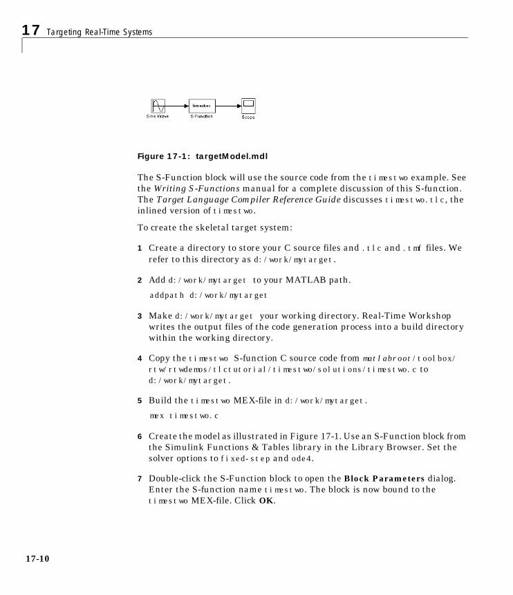
17 Targeting Real-Time Systems
17-10
Figure 17-1: targetModel.mdl
The S-Function block will use the source code from the timestwo example. Seethe Writing S-Functions manual for a complete discussion of this S-function.The Target Language Compiler Reference Guide discusses timestwo.tlc, theinlined version of timestwo.
To create the skeletal target system:
1 Create a directory to store your C source files and .tlc and .tmf files. Werefer to this directory as d:/work/mytarget.
2 Add d:/work/mytarget to your MATLAB path.
addpath d:/work/mytarget
3 Make d:/work/mytarget your working directory. Real-Time Workshopwrites the output files of the code generation process into a build directorywithin the working directory.
4 Copy the timestwo S-function C source code from matlabroot/toolbox/rtw/rtwdemos/tlctutorial/timestwo/solutions/timestwo.c tod:/work/mytarget.
5 Build the timestwo MEX-file in d:/work/mytarget.
mex timestwo.c
6 Create the model as illustrated in Figure 17-1. Use an S-Function block fromthe Simulink Functions & Tables library in the Library Browser. Set thesolver options to fixed-step and ode4.
7 Double-click the S-Function block to open the Block Parameters dialog.Enter the S-function name timestwo. The block is now bound to thetimestwo MEX-file. Click OK.
Tutorial: Creating a Custom Target Configuration
17-11
8 Open the Scope and run the simulation. Verify that the timestwo S-functionmultiplies its input by 2.0.
9 In order to generate inlined code from the timestwo S-Function block, youmust have a corresponding TLC file in the working directory. If the TargetLanguage Compiler detects a C-code S-function and a TLC file with thesame name in the working directory, it generates inline code from the TLCfile. Otherwise, it generates a function call to the external S-function.
To ensure that the build process generates inlined code from the timestwoblock, copy the timestwo TLC source code from matlabroot/toolbox/rtw/rtwdemos/tlctutorial/timestwo/solutions/timestwo.tlc tod:/work/mytarget.
10 Make local copies of the main program and system target files. matlabroot/rtw/c/grt contains the main program (grt_main.c) and the system targetfile (grt.tlc) for the generic real-time target. Copy grt_main.c and grt.tlcto d:/work/mytarget. Rename them to mytarget_main.c andmytarget.tlc.
11 Remove the initial comment lines from mytarget.tlc. The lines to removeare shown below.
%% SYSTLC: Generic Real-Time Target \%% TMF: grt_default_tmf MAKE: make_rtw EXTMODE: ext_comm %% SYSTLC: Visual C/C++ Project Makefile only for the "grt" target \%% TMF: grt_msvc.tmf MAKE: make_rtw EXTMODE: ext_comm
The initial comment lines have significance only if you want to addmy_target to the System Target File Browser. For now you should removethem.

17 Targeting Real-Time Systems
17-12
12 Real-Time Workshop creates a build directory in your working directory tostore files created during the code generation process. The build directory isgiven the name of the model, followed by a suffix. This suffix is specified inthe rtwgensettings structure in the system target file.
To set the suffix to a more appropriate string, change the line
rtwgensettings.BuildDirSuffix = '_grt_rtw'
to
rtwgensettings.BuildDirSuffix = '_mytarget_rtw'
Your build directory will be named targetModel__mytarget_rtw.
13 Make a local copy of the template makefile. matlabroot/rtw/c/grt containsseveral compiler-specific template makefiles for the generic real-time target.The appropriate template makefile for the LCC compiler is grt_lcc.tmf.Copy grt_lcc.tmf to d:/work/mytarget, and rename it to mytarget.tmf.
Note Some of the template makefile modifications described in the next stepare specific to the LCC template makefile. If you are using a different compilerand template makefile, the rules for the source (REQ_SRCS) and object file(%.obj :) lists may differ slightly.

Tutorial: Creating a Custom Target Configuration
17-13
14 Modify mytarget.tmf. The SYS_TARGET FILE parameter must be changed sothat the correct file reference is generated in the make file. Change the line
SYS_TARGET FILE = grt.tlc
to
SYS_TARGET FILE = mytarget.tlc
Also, change the source file list to include mytarget_main.c instead ofgrt_main.c.
REQ_SRCS = $(MODEL).c $(MODULES) mytarget_main.c...
Finally, change the line
%.obj : $(MATLAB_ROOT)/rtw/c/grt/%.c
to
%.obj : d:/work/mytarget/%.c
15 This exercise requires no changes to mytarget_main.c. In an actualapplication, you would modify mytarget_main.c to execute your model codeunder the control of a timer interrupt, and make other changes.
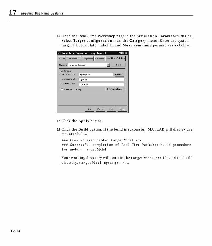
17 Targeting Real-Time Systems
17-14
16 Open the Real-Time Workshop page in the Simulation Parameters dialog.Select Target configuration from the Category menu. Enter the systemtarget file, template makefile, and Make command parameters as below.
17 Click the Apply button.
18 Click the Build button. If the build is successful, MATLAB will display themessage below.
### Created executable: targetModel.exe ### Successful completion of Real-Time Workshop build procedure for model: targetModel
Your working directory will contain the targetModel.exe file and the builddirectory, targetModel_mytarget_rtw.
Tutorial: Creating a Custom Target Configuration
17-15
19 Edit the generated file d:/work/mytarget/targetModel_mytarget_rtw/targetModel.c and locate the MdlOutputs function. Observe the inlinedcode.
/* S-Function Block: <Root>/S-Function (timestwo) */rtB.S_Function = 2.0 * rtB.Sine_Wave;
Because the working directory contained a TLC file (timestwo.tlc) withthe same name as the timestwo S-Function block, the Target LanguageCompiler generated inline code instead of a function call to the external C-code S-function.
20 As an optional final step to this exercise, you may want to add your customtarget configuration to the System Target File Browser. See “Adding aCustom Target to the System Target File Browser” on page 17-24 to learnhow to do this.
17 Targeting Real-Time Systems
17-16
Customizing the Build ProcessThe Real-Time Workshop build process proceeds in two stages. The first stageis code generation. The system target file exerts overall control of the codegeneration stage. In the second stage, the template makefile generates a .mk file, which compiles and links code modules into an executable.
In developing your custom target, you may need to create a customized systemtarget file and/or template makefile. This section provides information on thestructure of these files, and guidelines for modifying them.
System Target File StructureThis section is a guide to the structure and contents of a system target file. Youmay want to refer to the system target files provided with the Real-TimeWorkshop while reading this section. Most of these files are stored in thetarget-specific directories under matlabroot/rtw/c. Additional system targetfiles are stored in matlabroot/toolbox/rtw/targets/rtwin/rtwin andmatlabroot/toolbox/rtw/targets/xpc/xpc.
Before creating or modifying a system target file, you should acquire a workingknowledge of the Target Language Compiler. The Target Language CompilerReference Guide documents the features and syntax of the language.
Figure 17-2 shows the general structure of a system target file.
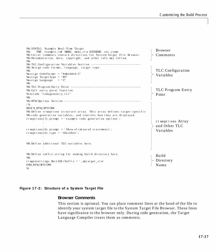
Customizing the Build Process
17-17
Figure 17-2: Structure of a System Target File
Browser CommentsThis section is optional. You can place comment lines at the head of the file toidentify your system target file to the System Target File Browser. These lineshave significance to the browser only. During code generation, the TargetLanguage Compiler treats them as comments.
%% SYSTLC: Example Real-Time Target%% TMF: example.tmf MAKE: make_rtw EXTMODE: ext_comm%% Inital comments contain directives for System Target File Browser.%% Documentation, date, copyright, and other info may follow.%%%% TLC Configuration Variables Section ------------------------------%% Assign code format, language, target type.%%%assign CodeFormat = "Embedded-C"%assign TargetType = "RT"%assign Language = "C"%%%% TLC Program Entry Point ------------------------------------------%% Call entry point function.%include "codegenentry.tlc"%%%% RTW Options Section ----------------------------------------------/%BEGIN_RTW_OPTIONS%% Define rtwoptions structure array. This array defines target-specific%% code generation variables, and controls how they are displayed.rtwoptions(1).prompt = 'example code generation options';
.
.rtwoptions(6).prompt = 'Show eliminated statements';rtwoptions(6).type = 'Checkbox';
.
.%% Define additional TLC variables here.
.
.%% Define suffix string for naming build directory here.%%rtwgensettings.BuildDirSuffix = '_mytarget_rtw'END_RTW_OPTIONS%/
BrowserComments
TLC ConfigurationVariables
TLC Program EntryPoint
rtwoptions Arrayand Other TLCVariables
BuildDirectoryName
17 Targeting Real-Time Systems
17-18
Note that you must place the browser comments at the head of the file, beforeany other comments or TLC statements.
The comments contain the following directives:
• SYSTLC: This string is a descriptor that appears in the browser.
• TMF: Name of the template makefile to use during build process. When thetarget is selected, this filename is displayed in the Template makefile fieldof the Target configuration section of the Real-Time Workshop page.
• MAKE: make command to use during build process. When the target is selected,this command is displayed in the Make command field of the Targetconfiguration section of the Real-Time Workshop page.
• EXTMODE: Name of external mode interface file (if any) associated with yourtarget. If your target does not support external mode, use no_ext_comm.
The following browser information comments are from matlabroot/rtw/c/grt/grt.tlc.
%% SYSTLC: Generic Real-Time Target %% TMF: grt_default_tmf MAKE: make_rtw EXTMODE: ext_comm
See “Adding a Custom Target to the System Target File Browser” on page17-24 for further information.
Target Language Compiler Configuration VariablesThis section assigns global TLC variables that affect the overall codegeneration process. The following variables must be assigned:
• CodeFormat: The CodeFormat variable selects one of the available codeformats:- RealTime: Designed for rapid prototyping, with static memory allocation.- RealTimeMalloc: Similar to RealTime, but with dynamic memory
allocation.- Embedded-C: Designed for production code, minimal memory usage,
simplified interface to generated code.- S-Function: For use by S-function and Accelerator targets only.
Customizing the Build Process
17-19
- Ada: Designed for production code, minimal memory usage, simplifiedinterface to generated code.
The default CodeFormat value is RealTime.
Chapter 4, “Generated Code Formats” summarizes available code formatsand provides pointers to further details.
• Language: Selects code generation in one of the supported languages:- C- Ada
When Ada is selected, Real-Time Workshop generates Ada95 code bydefault. To generate Ada83 code, set the variable AdaVersion as follows.
%assign AdaVersion = “83”
It is possible to generate code in a language other than C or Ada. To do thiswould require considerable development effort, including reimplementationof all block target files to generate the desired target language code. See theTarget Language Compiler Reference Guide for a discussion of the issues.
• TargetType: The Real-Time Workshop defines the preprocessor symbols RTand NRT to distinguish simulation code from real-time code. These symbolsare used in conditional compilation. The TargetType variable determineswhether RT or NRT is defined.
Most targets are intended to generate real-time code. They assignTargetType as follows.%assign TargetType = "RT"
Some targets, such as the Simulink Accelerator, generate code for use in nonreal-time only. Such targets assign TargetType as follows.%assign TargetType = "NRT"
See “Conditional Compilation for Simulink and Real-Time” on page 17–40for further information on the use of these symbols.
Target Language Compiler Program Entry PointThe code generation process normally begins with codegenentry.tlc. Thesystem target file invokes codegenentry.tlc as follows.
%include "codegenentry.tlc"
17 Targeting Real-Time Systems
17-20
codegenentry.tlc in turn invokes other TLC files:
• genmap.tlc maps the block names to corresponding language-specific blocktarget files.
• commonsetup.tlc sets up global variables.
• commonentry.tlc starts the process of generating code in the formatspecified by CodeFormat.
To customize the code generation process, you can call the lower-level TLC filesexplicitly and include your own TLC functions at each stage of the process. Seethe Target Language Compiler Reference Guide for guidelines.
Note codegenentry.tlc and the lower-level TLC files assume that CodeFormat, TargetType, and Language have been correctly assigned. Setthese variables before including codegenentry.tlc.
RTW_OPTIONS SectionThe RTW_OPTIONS section (see Figure 17-2) is bounded by the directives:
%/BEGIN_RTW_OPTIONS..END_RTW_OPTIONS/%
The first part of the RTW_OPTIONS section defines an array of rtwoptionsstructures. The rtwoptions structure is discussed in this section.
The second part of the RTW_OPTIONS section defines rtwgensettings, astructure defining the build directory name and other settings for the codegeneration process. See “Build Directory Name” on page 17-24 for informationabout rtwgensettings.
The rtwoptions Structure. The fields of the rtwoptions structure define variablesand associated user interface elements to be displayed in the Real-TimeWorkshop page. Using the rtwoptions structure array, you can customize theCategory menu in the Real-Time Workshop page, define the options displayedin each category, and specify how these options are processed.
Customizing the Build Process
17-21
When the Real-Time Workshop page opens, the rtwoptions structure array isscanned and the listed options are displayed. Each option is represented by anassigned user interface element (check box, edit field, pop-up menu, orpushbutton), which displays the current option value.
The user interface elements can be in an enabled or disabled (grayed-out) state.If the option is enabled, the user can change the option value.
The elements of the rtwoptions structure array are organized into groups thatcorrespond to items in the Category menu in the Real-Time Workshop page.Each group of items begins with a header element of type Category. Thedefault field of a Category header must contain a count of the remainingelements in the category.
The header is followed by options to be displayed on the Real-Time Workshoppage. The header in each category is followed by a maximum of seven elements.
Table 17-2 summarizes the fields of the rtwoptions structure.
The following example is excerpted from matlabroot/rtw/c/rtwsfcn/rtwsfcn.tlc, the system target file for the S-Function target. The code definesan rtwoptions structure array of three elements. The default field of the first(header) element is set to 2, indicating the number of elements that follow theheader.
rtwoptions(1).prompt = 'RTW S-function code generation options'; rtwoptions(1).type = 'Category'; rtwoptions(1).enable = 'on'; rtwoptions(1).default = 2; % Number of items under this category
% excluding this one.
rtwoptions(2).prompt = 'Create New Model'; rtwoptions(2).type = 'Checkbox'; rtwoptions(2).default = 'on'; rtwoptions(2).tlcvariable = 'CreateModel'; rtwoptions(2).makevariable = 'CREATEMODEL'; rtwoptions(2).tooltip = ... ['Create a new model containing the generated RTW S-Function block inside it'];
rtwoptions(3).prompt = 'Use Value for Tunable Parameters'; rtwoptions(3).type = 'Checkbox'; rtwoptions(3).default = 'off'; rtwoptions(3).tlcvariable = 'UseParamValues'; rtwoptions(3).makevariable = 'USEPARAMVALUES'; rtwoptions(3).tooltip = ...['Use value instead of variable name in generated block mask edit fields'];
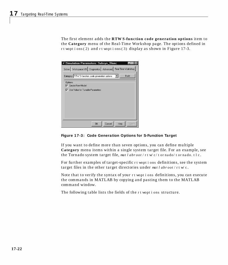
17 Targeting Real-Time Systems
17-22
The first element adds the RTW S-function code generation options item tothe Category menu of the Real-Time Workshop page. The options defined inrtwoptions(2) and rtwoptions(3) display as shown in Figure 17-3.
Figure 17-3: Code Generation Options for S-Function Target
If you want to define more than seven options, you can define multipleCategory menu items within a single system target file. For an example, seethe Tornado system target file, matlabroot/rtw/c/tornado/tornado.tlc.
For further examples of target-specific rtwoptions definitions, see the systemtarget files in the other target directories under matlabroot/rtw/c.
Note that to verify the syntax of your rtwoptions definitions, you can executethe commands in MATLAB by copying and pasting them to the MATLABcommand window.
The following table lists the fields of the rtwoptions structure.

Customizing the Build Process
17-23
Table 17-2: rtwoptions Structure Fields Summary
Field Name Description
callback Name of M-code function to call when value of optionchanges.
default Default value of the option (empty if the type isPushbutton).
enable Must be on or off. If on, the option is displayed as anenabled item; otherwise, as a disabled item.
makevariable Template makefile token (if any) associated withoption. The makevariable will be expanded duringprocessing of the template makefile. See “TemplateMakefile Tokens” on page 17-26.
opencallback M-code to be executed when dialog opens. The purposeof the code is to synchronize the displayed value of theoption with its previous setting. See matlabroot/rtw/c/ert/ert.tlc for an example.
popupstrings If type is Popup, popupstrings defines the items in thepop-up menu. Items are delimited by the “|” (verticalbar) character. The following example defines the itemsof the Function management menu used by the GRTand other targets:
['None|Function splitting|File ', ... 'splitting|Function and file splitting']
prompt Label for the option.
tlcvariable Name of TLC variable associated with the option.
tooltip Help string displayed when mouse is over the item.
type Type of element: Checkbox, Edit, Popup, Pushbutton, orCategory.

17 Targeting Real-Time Systems
17-24
Additional Code Generation Options“Target Language Compiler Variables and Options” on page 3-93 describesadditional code generation variables. For readability, it is recommended thatyou assign these variables in the Configure RTW code generation settingssection of the system target file.
Alternatively, you can append statements of the form
-aVariable=val
to the System target filename field on the Real-Time Workshop page.
Build Directory NameThe final part of the system target file defines the BuildDirSuffix field of thertwgensettings structure. The build process appends the BuildDirSuffixstring to the model name to form the name of the build directory. For example,if you define BuildDirSuffix as follows
rtwgensettings.BuildDirSuffix = '_mytarget_rtw'
the build directories are named model_mytarget_rtw.
See the Target Language Compiler Reference Manual for further informationon the rtwgensettings structure.
Adding a Custom Target to the System TargetFile BrowserAs a convenience to end users of your custom target configuration, you can adda custom target configuration to the System Target File Browser. To do this:
1 Modify (or add) browser comments at the head of your custom system targetfile. For example,
%% SYSTLC: John’s Real-Time Target \%% TMF: mytarget.tmf MAKE: make_rtw EXTMODE: no_ext_comm
2 Create a directory <targetname> (e.g., /mytarget). Move your custom systemtarget file, custom template makefile, and run-time interface files (such asyour main program and S-functions) into the <targetname> subdirectory.
3 Add your target directory to the MATLAB path.

Customizing the Build Process
17-25
addpath <targetname>
If you want <targetname> included in the MATLAB path each timeMATLAB starts up, include this addpath command in your startup.m file.
4 When the System Target File Browser opens, Real-Time Workshop detectssystem target files that are on the MATLAB path, and displays the targetfilenames and target description comments. Figure 17-4 shows how thetarget file mytarget.tlc, which contains the browser comments above,appears in the System Target File Browser.
Figure 17-4: Custom System Target File Displayed in Browser
Template MakefilesTo configure or customize template makefiles, you should be familiar with howthe make command works and how the make command processes makefiles. Youshould also understand makefile build rules. For information of these topics,please refer to the documentation provided with the make utility you use.There are also several good books on the make utility.
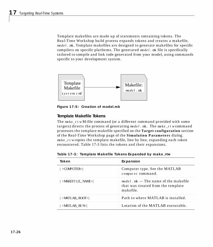
17 Targeting Real-Time Systems
17-26
Template makefiles are made up of statements containing tokens. TheReal-Time Workshop build process expands tokens and creates a makefile,model.mk. Template makefiles are designed to generate makefiles for specificcompilers on specific platforms. The generated model.mk file is specificallytailored to compile and link code generated from your model, using commandsspecific to your development system.
Figure 17-5: Creation of model.mk
Template Makefile TokensThe make_rtw M-file command (or a different command provided with sometargets) directs the process of generating model.mk. The make_rtw command processes the template makefile specified on the Target configuration sectionof the Real-Time Workshop page of the Simulation Parameters dialog.make_rtw copies the template makefile, line by line, expanding each tokenencountered. Table 17-3 lists the tokens and their expansions.
Table 17-3: Template Makefile Tokens Expanded by make_rtw
Token Expansion
|>COMPUTER<| Computer type. See the MATLABcomputer command.
|>MAKEFILE_NAME<| model.mk — The name of the makefilethat was created from the templatemakefile.
|>MATLAB_ROOT<| Path to where MATLAB is installed.
|>MATLAB_BIN<| Location of the MATLAB executable.
TemplateMakefile
Makefile:model.mk
system.tmf

Customizing the Build Process
17-27
|>MEM_ALLOC<| Either RT_MALLOC or RT_STATIC.Indicates how memory is to be allocated.
|>MEXEXT<| MEX-file extension. See the MATLABmexext command.
|>MODEL_NAME<| Name of the Simulink block diagramcurrently being built.
|>MODEL_MODULES<| Any additional generated source (.c)modules. For example, you can split alarge model into two files, model.c andmodel1.c. In this case, this tokenexpands to model1.c.
|>MODEL_MODULES_OBJ<| Object filenames (.obj) correspondingto any additional generated source (.c)modules.
|>MULTITASKING<| True (1) if solver mode is multitasking,otherwise False (0).
|>NUMST<| Number of sample times in the model.
|>RELEASE_VERSION<| The release version of MATLAB.
|>S_FUNCTIONS<| List of noninlined S-function (.c)sources.
|>S_FUNCTIONS_LIB<| List of S-function libraries available forlinking.
|>S_FUNCTIONS_OBJ<| Object (.obj) file list corresponding tononinlined S-function sources.
|>SOLVER<| Solver source filename, e.g., ode3.c.
|>SOLVER_OBJ<| Solver object (.obj) filename, e.g.,ode3.obj.
Table 17-3: Template Makefile Tokens Expanded by make_rtw (Continued)
Token Expansion

17 Targeting Real-Time Systems
17-28
These tokens are expanded by substitution of parameter values known to thebuild process. For example, if the source model contains blocks with twodifferent sample times, the template makefile statement
NUMST = |>NUMST<|
expands to the following in model.mk.
NUMST = 2
In addition to the above, make_rtw expands tokens from other sources:
• Target-specific tokens defined via the Target configuration section of theReal-Time Workshop page of the Simulation Parameters dialog box.
• Structures in the RTW Options section of the system target file. Anystructures in the rtwoptions structure array that contain the fieldmakevariable are expanded.
The following example is extracted from matlabroot/rtw/c/grt/grt.tlc. The section starting with BEGIN_RTW_OPTIONS contains M-file code that setsup rtwoptions. The directive
|>TID01EQ<| True (1) if sampling rates of thecontinuous task and the first discretetask are equal, otherwise False (0).
|>NCSTATES<| Number of continuous states.
|>BUILDARGS<| Options passed to make_rtw. This tokenis provided so that the contents of yourmodel.mk file will change when youchange the build arguments, thusforcing an update of all modules whenyour build options change.
|>EXT_MODE<| True (1) to enable generation ofexternal mode support code, otherwiseFalse (0).
Table 17-3: Template Makefile Tokens Expanded by make_rtw (Continued)
Token Expansion

Customizing the Build Process
17-29
rtwoptions(2).makevariable = 'EXT_MODE'
causes the |>EXT_MODE<| token to be expanded into 1 (on) or 0 (off),depending on how you set the External mode option in the Code generationoptions section of the Real-Time Workshop page.
The Make CommandAfter creating model.mk from your template makefile, the Real-Time Workshopinvokes a make command. To invoke make, the Real-Time Workshop issues thiscommand.
makecommand -f model.mk
makecommand is defined by the MAKE macro in your system’s template makefile(see Figure 17-6 on page 17-31). You can specify additional options to make inthe Make command field of the Real-Time Workshop page. (see “MakeCommand Field” on page 3-8 and “Template Makefiles and Make Options” onpage 3-102.)
For example, specifying OPT_OPTS=-O2 in the Make command field causesmake_rtw to generate the following make command.
makecommand -f model.mk OPT_OPTS=-O2
A comment at the top of the template makefile specifies the available makecommand options. If these options do not provide you with enough flexibility,you can configure your own template makefile.
Make Utilities
The make utility lets you control nearly every aspect of building your real-timeprogram. There are several different versions of make available. The Real-TimeWorkshop provides the Free Software Foundation’s GNU Make for both UNIXand PC platforms in the platform-specific subdirectories below matlabroot/rtw/bin.
It is possible to use other versions of make with the Real-Time Workshop,although GNU Make is recommended. To ensure compatibility with theReal-Time Workshop, make sure that your version of make supports thefollowing command format.
makecommand −f model.mk
17 Targeting Real-Time Systems
17-30
Structure of the Template MakefileA template makefile has four sections:
• The first section contains initial comments that describe what this makefiletargets.
• The second section defines macros that tell make_rtw how to process thetemplate makefile. The macros are:
- MAKE — This is the command used to invoke the make utility. For example,if MAKE = mymake, then the make command invoked is
mymake −f model.mk- HOST — What platform this template makefile is targeted for. This can beHOST=PC, UNIX, computer_name (see the MATLAB computer command), orANY.
- BUILD — This tells make_rtw whether or not (BUILD=yes or no) it shouldinvoke make from the Real-Time Workshop build procedure.
- SYS_TARGET_FILE — Name of the system target file. This is used forconsistency checking by make_rtw to verify that the correct system targetfile was specified in the Target configuration section of the Real-TimeWorkshop page of the Simulation Parameters dialog box.
- BUILD_SUCCESS— An optional macro that specifies the build success stringto be displayed on successful make completion on the PC. For example,BUILD_SUCCESS = ### Successful creation of
- BUILD_ERROR — An optional macro that specifies the build error messageto be displayed when an error is encountered during the make procedure.For example,BUILD_ERROR = ['Error while building ', modelName]
The following DOWNLOAD options apply only to the Tornado target:- DOWNLOAD — An optional macro that you can specify as yes or no. If
specified as yes (and BUILD=yes), then make is invoked a second time withthe download target.
make -f model.mk download
- DOWNLOAD_SUCCESS — An optional macro that you can use to specify thedownload success string to be used when looking for a successfuldownload. For example,
DOWNLOAD_SUCCESS = ### Downloaded
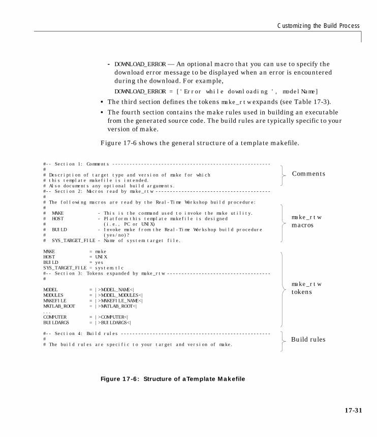
Customizing the Build Process
17-31
- DOWNLOAD_ERROR — An optional macro that you can use to specify thedownload error message to be displayed when an error is encounteredduring the download. For example,
DOWNLOAD_ERROR = ['Error while downloading ', modelName]
• The third section defines the tokens make_rtw expands (see Table 17-3).
• The fourth section contains the make rules used in building an executablefrom the generated source code. The build rules are typically specific to yourversion of make.
Figure 17-6 shows the general structure of a template makefile.
Figure 17-6: Structure of aTemplate Makefile
#-- Section 1: Comments -------------------------------------------------------## Description of target type and version of make for which # this template makefile is intended.# Also documents any optional build arguments.#-- Section 2: Macros read by make_rtw ----------------------------------------## The following macros are read by the Real-Time Workshop build procedure:## MAKE - This is the command used to invoke the make utility.# HOST - Platform this template makefile is designed # (i.e., PC or UNIX)# BUILD - Invoke make from the Real-Time Workshop build procedure # (yes/no)?# SYS_TARGET_FILE - Name of system target file.
MAKE = makeHOST = UNIXBUILD = yesSYS_TARGET_FILE = system.tlc#-- Section 3: Tokens expanded by make_rtw ------------------------------------#
MODEL = |>MODEL_NAME<|MODULES = |>MODEL_MODULES<|MAKEFILE = |>MAKEFILE_NAME<|MATLAB_ROOT = |>MATLAB_ROOT<|...COMPUTER = |>COMPUTER<|BUILDARGS = |>BUILDARGS<|
#-- Section 4: Build rules ----------------------------------------------------## The build rules are specific to your target and version of make.
Comments
make_rtwmacros
make_rtwtokens
Build rules
17 Targeting Real-Time Systems
17-32
Customizing and Creating Template MakefilesTo customize or create a new template makefile, we recommend that you copyan existing template makefile to your local working directory and modify it.
This section shows, through an example, how to use macros andfile-pattern-matching expressions in a template makefile to generatecommands in the model.mk file.
The make utility processes the model.mk makefile and generates a set ofcommands based upon dependency rules defined in model.mk. After makegenerates the set of commands needed to build or rebuild test, make executesthem.
For example, to build a program called test, make must link the object files.However, if the object files don’t exist or are out of date, make must compile theC code. Thus there is a dependency between source and object files.
Each version of make differs slightly in its features and how rules are defined.For example, consider a program called test that gets created from twosources, file1.c and file2.c. Using most versions of make, the dependencyrules would be
test: file1.o file2.occ −o test file1.o file2.o
file1.o: file1.ccc −c file1.c
file2.o: file2.ccc −c file2.c
In this example, we assumed a UNIX environment. In a PC environment thefile extensions and compile and link commands will be different.
In processing the first rule
test: file1.o file2.o
make sees that to build test, it needs to build file1.o and file2.o. To buildfile1.o, make processes the rule
file1.o: file1.c
Customizing the Build Process
17-33
If file1.o doesn’t exist, or if file1.o is older than file1.c, make compilesfile1.c.
The format of Real-Time Workshop template makefiles follows the aboveexample. Our template makefiles use additional features of make such asmacros and file-pattern-matching expressions. In most versions of make, amacro is defined via
MACRO_NAME = value
References to macros are made via $(MACRO_NAME). When make sees this formof expression, it substitutes value for $(MACRO_NAME).
You can use pattern matching expressions to make the dependency rules moregeneral. For example, using GNU Make you could replace the two "file1.o: file1.c" and "file2.o: file2.c" rules with the single rule
%.o : %.ccc −c $<
Note that $< above is a special macro that equates to the dependency file (i.e.,file1.c or file2.c). Thus, using macros and the “%” pattern matchingcharacter, the above example can be reduced to
SRCS = file1.c file2.cOBJS = $(SRCS:.c=.o)
test: $(OBJS)cc −o $@ $(OBJS)
%.o : %.ccc −c $<
Note that the $@macro above is another special macro that equates to the nameof the current dependency target, in this case test.
This example generates the list of objects (OBJS) from the list of sources (SRCS)by using the string substitution feature for macro expansion. It replaces thesource file extension (.c) with the object file extension (.o). This example alsogeneralized the build rule for the program, test, to use the special “$@” macro.
17 Targeting Real-Time Systems
17-34
Creating Device DriversDevice drivers that communicate with target hardware are essential to manyreal-time development projects. This section describes how to integrate devicedrivers into your target system. This includes incorporating drivers into yourSimulink model and into the code generated from that model.
Device drivers are implemented as Simulink device driver blocks. A devicedriver block is an S-Function block that is bound to user-written driver code.
To implement device drivers, you should be familiar with the Simulink C MEXS-function format and API. The following documents contain more informationabout C MEX S-functions:
• Writing S-Functions describes S-functions, including how to write bothinlined and noninlined S-functions and how to access parameters from amasked S-function. Writing S-Functions also describes how to use the specialmdlRTW function to parameterize an inlined S-function.
• “External Interfaces” in the MATLAB online documentation explains how towrite C and other programs that interact with MATLAB via the MEX API.Simulink’s S-function API is built on top of this API. To pass parameters toyour device driver block from MATLAB/Simulink you must use the MEXAPI. MATLAB Application Program Interface Reference Guide containsreference descriptions for the required MATLAB mx* routines.
• Target Language Compiler Reference Guide describes the Target LanguageCompiler. Knowledge of the Target Language Compiler is required in orderto inline S-functions. The Target Language Compiler Reference Guide alsodescribes the structure of the model.rtw file.
• “Using Masks to Customize Blocks” in Using Simulink describes how tocreate a mask for an S-function.
Note Device driver blocks must be implemented as C MEX S-functions, notas M-file S-functions. C MEX S-functions are limited to a subset of thefeatures available in M-file S-functions. See “Limitations of Device DriverBlocks” on page 17-37 for information.
Creating Device Drivers
17-35
This section covers the following topics:
• Inlined and noninlined device drivers
• General requirements and limitations for device drivers
• Obtaining S-function parameter values from a dialog box
• Writing noninlined device drivers
• Writing inlined device drivers
• Building the device driver MEX-file
Inlined and Noninlined DriversIn your target system, a device driver has a dual function. First, it functions asa code module that you compile and link with other code generated from yourmodel by Real-Time Workshop. In addition, the driver must interact withSimulink during simulation. To meet both these requirements, you mustincorporate your driver code into a Simulink device driver block.
You can build your driver S-function in several ways:
• As a MEX-file component, bound to an S-Function block, for use in aSimulink model. In this case, the Simulink engine calls driver routines in theMEX-file during execution of the model.
• As a module within a stand-alone real-time program that is generated froma model by Real-Time Workshop. The driver routines are called from withinthe application in essentially the same way that Simulink calls them.
In many cases, the code generated from driver blocks for real-time executionmust run differently from the code used by the blocks in simulation. Forexample, an output driver may write to hard device addresses in real time;but these write operations could cause errors in simulation.
Real-Time Workshop provides standard compilation conditionals andinclude files to let you build the drivers for both cases. (See “ConditionalCompilation for Simulink and Real-Time” on page 17-40.)
• As inlined code. The Target Language Compiler enables you to generate theexplicit code from your routines (instead of calls to these routines) in the bodyof the application. Inlined code eliminates calling overhead, and reducesmemory usage.
Inlining an S-function can improve its performance significantly. However,there is a tradeoff in increased development and maintenance effort. To inline
17 Targeting Real-Time Systems
17-36
a device driver block, you must implement the block twice: first, as a CMEX-file, and second, as a TLC program.
The C MEX-file version is for use in simulation. Since a simulation normallydoes not have access to I/O boards or other target hardware, the C MEX-fileversion often acts as a “dummy” block within a model. For example, adigital-to-analog converter (DAC) device driver block is often implemented asa stub for simulation.
Alternatively, the C MEX-file version can simulate the behavior of thehardware. For example, an analog-to-digital converter (ADC) device driverblock might read sample values from a data file or from the MATLABworkspace.
The TLC version generates actual working code that accesses the targethardware in a production system.
Inlined device drivers are an appropriate design choice when:
• You are using the Real-Time Workshop Embedded Coder target. InlinedS-functions are required when building code from the Real-Time WorkshopEmbedded Coder target. S-functions for other targets can be either inlinedor noninlined.
• You need production code generated from the S-function to behavedifferently than code used during simulation. For example, an output deviceblock may write to an actual hardware address in generated code, butperform no output during simulation.
• You want to avoid overhead associated with calling the S-function API.
• You want to reduce memory usage. Note that each noninlined S-functioncreates its own Simstruct. Each Simstruct uses over 1K of memory. InlinedS-functions do not allocate any Simstruct. For optimal memory usage,consider using inlined S-functions with the Real-Time Workshop EmbeddedCoder target.
• You want to avoid making calls to routines that are required by Simulink,but which are empty, in your generated code.
Creating Device Drivers
17-37
Device Driver Requirements and LimitationsIn order to create a device driver block, the following components are required:
• Hardware-specific driver code, which handles communication between areal-time program and an I/O device. See your I/O device documentation forinformation on hardware requirements.
• S-function code, which implements the model initialization, output, andother functions required by the S-function API. The S-function code callsyour driver code.
Your S-function code and the hardware-specific driver code are compiled andlinked into a component that is bound to an S-Function block in yourSimulink model. The MATLAB mex utility builds this component (a DLLunder Windows, or a shared library under UNIX).
We recommend that you use the S-function template provided by theReal-Time Workshop as a starting point for developing your driver S-functions.The template file is
matlabroot/simulink/src/sfuntmpl.c
An extensively commented version of the S-function template is also available.See matlabroot/simulink/src/sfuntmpl.doc.
The following components are optional:
• A TLC file that generates inline code for the S-function.
• A mask for the device driver block to create a customized user interface.
Limitations of Device Driver BlocksThe following limitations apply to noninlined driver blocks:
• Only a subset of MATLAB API functions are supported. See the “NoninlinedS-functions” section of Chapter 4 of Writing S-Functions for a complete listof supported calls.
• Parameters must be doubles or characters contained in scalars, vectors, or2-D matrices.
The following applies to inlined driver blocks:• If the driver does not have a mdlRTW function, parameter restrictions are the
same as for noninlined drivers.
• If the driver has a mdlRTW function, any parameter type is supported.
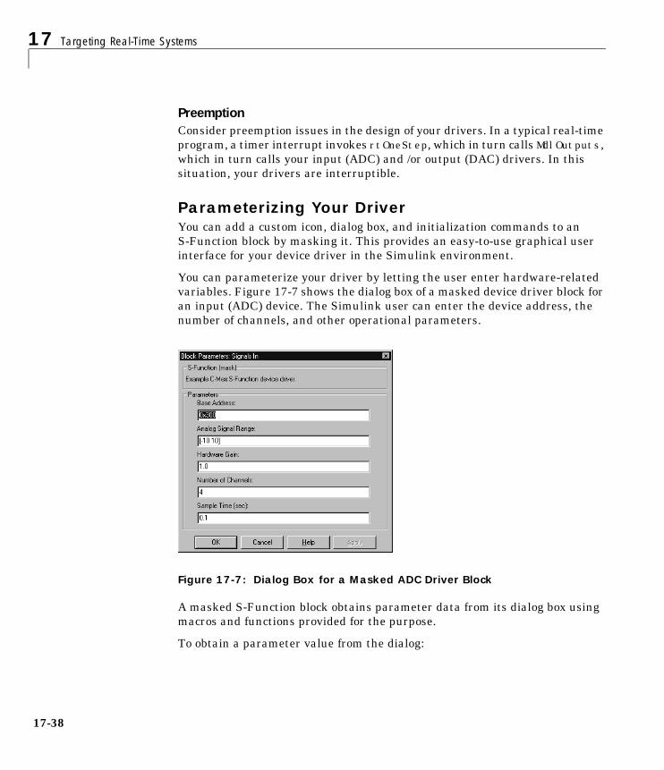
17 Targeting Real-Time Systems
17-38
PreemptionConsider preemption issues in the design of your drivers. In a typical real-timeprogram, a timer interrupt invokes rtOneStep, which in turn calls MdlOutputs,which in turn calls your input (ADC) and /or output (DAC) drivers. In thissituation, your drivers are interruptible.
Parameterizing Your DriverYou can add a custom icon, dialog box, and initialization commands to anS-Function block by masking it. This provides an easy-to-use graphical userinterface for your device driver in the Simulink environment.
You can parameterize your driver by letting the user enter hardware-relatedvariables. Figure 17-7 shows the dialog box of a masked device driver block foran input (ADC) device. The Simulink user can enter the device address, thenumber of channels, and other operational parameters.
Figure 17-7: Dialog Box for a Masked ADC Driver Block
A masked S-Function block obtains parameter data from its dialog box usingmacros and functions provided for the purpose.
To obtain a parameter value from the dialog:
Creating Device Drivers
17-39
1 Access the parameter from the dialog box using the ssGetSFcnParam macro.The arguments to ssGetSFcnParam are a pointer to the block’s Simstruct,and the index (0-based) to the desired parameter. For example, use thefollowing call to access the Number of Channels parameter from the dialogabove.
ssGetSFcnParam(S,3); /* S points to block’s Simstruct */
2 Parameters are stored in arrays of type mxArray, even if there is only asingle value. Get a particular value from the input mxArray using themxGetPr function. The following code fragment extracts the first (and only)element in the Number of Channels parameter.
#define NUM_CHANNELS_PARAM (ssGetSFcnParam(S,3))#define NUM_CHANNELS ((uint_T) mxGetPr(NUM_CHANNELS_PARAM)[0])uint_T num_channels;num_channels = NUM_CHANNELS;
It is typical for a device driver block to read and validate input parameters inits mdlInitializeSizes function. See the listing “adc.c” on page 17-55 for anexample.
By default, S-function parameters are tunable. To make a parameternontunable, use the ssSetSFcParamNotTunable macro in themdlInitializeSizes routine. Nontunable S-function parameters becomeconstants in the generated code, improving performance.
For further information on creation and use of masked blocks, see the UsingSimulink and Writing S-Functions manuals.
Writing a Noninlined S-Function Device Driver
OverviewDevice driver S-functions are relatively simple to implement because theyperform only a few operations. These operations include:
• Initializing the SimStruct.
• Initializing the I/O device.
• Calculating the block outputs. How this is done depends upon the type ofdriver being implemented:
17 Targeting Real-Time Systems
17-40
- An input driver for a device such as an ADC reads values from an I/Odevice and assigns these values to the block’s output vector y.
- An output driver for a device such as a DAC writes values from the block’sinput vector u to an I/O device.
• Terminating the program. This may require setting hardware to a “neutral”state; for example, zeroing DAC outputs.
Your driver performs these operations by implementing certain specificfunctions required by the S-function API.
Since these functions are private to the source file, you can incorporatemultiple instances of the same S-function into a model. Note that each suchnoninlined S-function also instantiates a SimStruct.
Conditional Compilation for Simulink and Real-TimeNoninlined S-functions must function in both Simulink and in real-timeenvironments. The Real-Time Workshop defines the preprocessor symbolsMATLAB_MEX_FILE, RT, and NRT to distinguish simulation code from real-timecode. Use these symbols as follows:
• MATLAB_MEX_FILE
Conditionally include code that is intended only for use in simulation underthis symbol. When you build your S-function as a MEX-file via the mexcommand, MATLAB_MEX_FILE is automatically defined.
• RT
Conditionally include code that is intended to run only in a real-timeprogram under this symbol. When you generate code via the Real-TimeWorkshop build command, RT is automatically defined.
• NRT
Conditionally include code that is intended only for use with a variable-stepsolver, in a non-real-time standalone simulation or in a MEX-file for use withSimulink, under this symbol.
Real-Time Workshop provides these conditionals to help ensure that yourdriver S-functions access hardware only when it is appropriate to do so. Sinceyour target I/O hardware is not present during simulation, writing toaddresses in the target environment can result in illegal memory references,overwriting system memory, and other severe errors. Similarly, read

Creating Device Drivers
17-41
operations from nonexistent hardware registers can cause model executionerrors.
In the following code fragment, a hardware initialization call is compiled ingenerated real-time code. During simulation, a message is printed to theMATLAB command window.
#if defined(RT)/* generated code calls function to initialize an A/D device */INIT_AD();
#elif defined(MATLAB_MEX_FILE)/* during simulation, just print a message */if (ssGetSimMode(S) == SS_SIMMODE_NORMAL) {mexPrintf("\n adc.c: Simulating initialization\n”);
}#endif
The MATLAB_MEX_FILE and RT conditionals also control the use of certainrequired include files. See “Required Defines and Include Files” below.
You may prefer to control execution of real-time and simulation code by someother means. For an example, see the use of the variable ACCESS_HW inmatlabroot/rtw/c/dos/devices/das16ad.c
Required Defines and Include FilesYour driver S-function must begin with the following three statements, in thefollowing order:
1 #define S_FUNCTION_NAME name
This defines the name of the entry point for the S-function code. name mustbe the name of the S-function source file, without the .c extension. Forexample, if the S-function source file is das16ad.c:
#define S_FUNCTION_NAME das16ad
2 #define S_FUNCTION_LEVEL 2
This statement defines the file as a level 2 S-function. This allows you totake advantage of the full feature set included with S-functions. Level-1S-functions are currently used only to maintain backwards compatibility.
17 Targeting Real-Time Systems
17-42
3 #include “simstruc.h”
The file simstruc.h defines the SimStruct (the Simulink data structure)and associated accessor macros. It also defines access methods for the mx*functions from the MATLAB MEX API.
Depending upon whether you intend to build your S-function as a MEX file oras real-time code, you must include one of the following files at the end of yourS-function:
• simulink.c provides required functions interfacing to Simulink.
• cg_sfun.h provides the required S-function entry point for generated code.
A noninlined S-function should conditionally include both these files, as in thefollowing code from sfuntmpl.c:
#ifdef MATLAB_MEX_FILE /* File being compiled as a MEX-file? */#include "simulink.c" /* MEX-file interface mechanism */#else#include "cg_sfun.h" /* Code generation registration function */#endif
Required FunctionsThe S-function API requires you to implement several functions in your driver:
• mdlInitializeSizes specifies the sizes of various parameters in theSimStruct, such as the number of output ports for the block.
• mdlInitializeSampleTimes specifies the sample time(s) of the block.
If your device driver block is masked, your initialization functions can obtainthe sample time and other parameters entered by the user in the block’sdialog box.
• mdlOutputs: for an input device, reads values from the hardware and setsthese values in the output vector y. For an output device, reads the input ufrom the upstream block and outputs the value(s) to the hardware.
• mdlTerminate resets hardware devices to a desired state, if any. Thisfunction may be implemented as a stub.
In addition to the above, you may want to implement the mdlStart function.mdlStart, which is called once at the start of model execution, is useful foroperations such as setting I/O hardware to some desired initial state.
This following sections provide guidelines for implementing these functions.
Creating Device Drivers
17-43
mdlInitializeSizes In this function you specify the sizes of various parameters in the SimStruct.This information may depend upon the parameters passed to the S-function.“Parameterizing Your Driver” on page 17-38 describes how to access parametervalues specified in S-function dialog boxes.
Initializing Sizes - Input Devices. The mdlInitializeSizes function sets sizeinformation in the SimStruct. The following implementation ofmdlInitializeSizes initializes a typical ADC driver block.
static void mdlInitializeSizes(SimStruct *S){uint_T num_channels;
ssSetNumSFcnParams(S, 3); /* Number of expected parameters */if (ssGetNumSFcnParams(S) != ssGetSFcnParamsCount(S)){ /*Return if number of expected != number of actual params */ return; }num_channels = mxGetPr(NUM_CHANNELS_PARAM)[0];
ssSetNumInputPorts(S, 0);ssSetNumOutputPorts(S, num_channels);ssSetNumSampleTimes(S,1);}
This routine first validates that the number of input parameters is equal to thenumber of parameters in the block’s dialog box. Next, it obtains the Number ofChannels parameter from the dialog.
ssSetNumInputPorts sets the number of input ports to 0 because an ADC is asource block, having only outputs.
ssSetNumOutputPorts sets the number of output ports equal to the number ofI/O channels obtained from the dialog box.
ssSetNumSampleTimes sets the number of sample times to 1. This would be thecase where all ADC channels run at the same rate. Note that the actual sampleperiod is set in mdlInitializeSampleTimes.
17 Targeting Real-Time Systems
17-44
Note that by default, the ADC block has no direct feedthrough. The ADC outputis calculated based on values read from hardware, not from data obtained fromanother block.
Initializing Sizes - Output Devices. Initializing size information for an outputdevice, such as a DAC, differs in several important ways from initializing sizesfor an ADC:
• Since the DAC obtains its inputs from other blocks, the number of channelsis equal to the number of inputs.
• The DAC is a sink block. That is, it has input ports but no output ports. Itsoutput is written to a hardware device.
• The DAC block has direct feedthrough. The DAC block cannot execute untilthe block feeding it updates its outputs.
The following example is an implementation of mdlInitializeSizes for a DACdriver block.
static void mdlInitializeSizes(SimStruct *S){uint_T num_channels;
ssSetNumSFcnParams(S, 3); /* Number of expected parameters */if (ssGetNumSFcnParams(S) != ssGetSFcnParamsCount(S)){ /* Return if number of expected != number of actual params */ return; }num_channels = mxGetPr(NUM_CHANNELS_PARAM)[0];ssSetNumInputPorts(S, num_channels);/* Number of inputs is now the number of channels. */ssSetNumOutputPorts(S, 0);/* Set direct feedthrough for all ports */ { uint_T i; for(i=0, i < num_channels, i++) { ssSetInputPortDirectFeedThrough(S,i,1); } }ssSetNumSampleTimes(S, 1);}
Creating Device Drivers
17-45
mdlInitializeSampleTimesDevice driver blocks are discrete blocks, requiring you to set a sample time. Theprocedure for setting sample times is the same for both input and output devicedrivers. Assuming that all channels of the device run at the same rate, theS-function has only one sample time.
The following implementation of mdlInitializeSampleTimes reads the sampletime from a block’s dialog box. In this case, sample time is the fifth parameterin the dialog box. The sample time offset is set to 0.
static void mdlInitializeSampleTimes(SimStruct *S){ssSetSampleTime(S, 0, mxGetPr(ssGetSFcnParams(S,4))[0]);ssSetOffsetTime(S, 0, 0.0);}
mdlStartmdlStart is an optional function. It is called once at the start of modelexecution, and is often used to initialize hardware. Since it accesses hardware,you should compile it conditionally for use in real-time code or simulation, asin this example:
static void mdlStart(SimStruct *S){#if defined(RT) /* Generated code calls function to initialize an A/D device */ INIT_AD(); /* This call accesses hardware */#elif defined(MATLAB_MEX_FILE) /* During simulation, just print a message */ if (ssGetSimMode(S) == SS_SIMMODE_NORMAL) { mexPrintf("\n adc.c: Simulating initialization\n"); }#endif}
mdlOutputsThe basic purpose of a device driver block is to allow your program tocommunicate with I/O hardware. Typically, you accomplish this by using lowlevel hardware calls that are part of your compiler’s C library, or by usingC-callable functions provided with your I/O hardware.

17 Targeting Real-Time Systems
17-46
All S-functions implement a mdlOutputs function to calculate block outputs.For a device driver block, mdlOutputs contains the code that reads from orwrites to the hardware.
mdlOutputs - Input Devices. In a driver for an input device (such as an ADC),mdlOutputs must:
• Initiate a conversion for each channel.
• Read the board’s ADC output for each channel (and perhaps apply scaling tothe values read).
• Set these values in the output vector y for use by the model.
The following code is the mdlOutputs function from the ADC drivermatlabroot/rtw/c/dos/devices/das16ad.c. The function uses macrosdefined in matlabroot/rtw/c/dos/devices/das16ad.h to perform low-levelhardware access. Note that the Boolean variable ACCESS_HW (rather thanconditional compilation) controls execution of simulation and real-time code.The real-time code reads values from the hardware and stores them to theoutput vector. The simulation code simply outputs 0 on all channels.
static void mdlOutputs(SimStruct *S, int_T tid){real_T *y = ssGetOutputPortRealSignal(S,0);uint_T i;if (ACCESS_HW) { /* Real-time code reads hardware*/ ADCInfo *adcInfo = ssGetUserData(S); uint_T baseAddr = adcInfo->baseAddr; real_T offset = adcInfo->offset; real_T resolution = adcInfo->resolution; /* For each ADC channel initiate conversion,*/ /* then read channel value, scale and offset it and store */ /* it to output y */ for (i = 0; i < NUM_CHANNELS; i++) { uint_T adcValue; adcStartConversion(baseAddr); for ( ; ; ){ if (!adcIsBusy(baseAddr)) break; } adcValue = adcGetValue(baseAddr);
Creating Device Drivers
17-47
y[i] = offset + resolution*adcValue; } }else { /* simulation code just zeroes the output for all channels*/ for (i = 0; i < NUM_CHANNELS; i++){ y[i] = 0.0; } }}
mdlOutputs - Output Devices. In a driver for an output device (such as a DAC),mdlOutputs must:
• Read the input u from the upstream block.
• Set the board’s DAC output for each channel (and apply scaling to the inputvalues if necessary).
• Initiate a conversion for each channel.
The following code is the mdlOutputs function from the DAC drivermatlabroot/rtw/c/dos/devices/das16da.c. The function uses macrosdefined in matlabroot/rtw/c/dos/devices/das16ad.h to perform low-levelhardware access. This function iterates over all channels, obtaining andscaling a block input value. It then range-checks and (if necessary) trims eachvalue. Finally it writes the value to the hardware.
In simulation, this function is a stub.
static void mdlOutputs(SimStruct *S, int_T tid){if (ACCESS_HW) { int_T i; DACInfo *dacInfo = ssGetUserData(S); uint_T baseAddr = dacInfo->baseAddr; real_T resolution = dacInfo->resolution; InputRealPtrsType uPtrs = ssGetInputPortRealSignalPtrs(S,0); for (i = 0; i < NUM_CHANNELS; i++) { uint_T codeValue; /* Get and scale input for channel i. */ real_T value = (*uPtrs[i] - MIN_OUTPUT)*resolution; /* Range check value */
17 Targeting Real-Time Systems
17-48
value = (value < DAC_MIN_OUTPUT) ? DAC_MIN_OUTPUT : value; value = (value > DAC_MAX_OUTPUT) ? DAC_MAX_OUTPUT : value; codeValue = (uint_T) value; /* Output to hardware */ switch (i) {case 0: dac0SetValue(baseAddr, codeValue); break; case 1: dac1SetValue(baseAddr, codeValue); break; } } }}
mdlTerminateThis final required function is typically needed only in DAC drivers. Thefollowing routine sets the output of each DAC channel to zero:
static void mdlTerminate(SimStruct *S){uint_T num_channels;uint_T i;
num_channels = (uint_t)mxGetPr(ssGetSFcnParams(S,0)[0]);for (i = 0; i < num_channels; i++){ ds1102_da(i + 1, 0.0); /* Hardware-specific DAC output */ }}
ADC drivers usually implement mdlTerminate as an empty stub.
Writing an Inlined S-Function Device Driver
OverviewTo inline a device driver, you must provide:
• driver.c: C MEX S-function source code, implementing the functionsrequired by the S-function API. These are the same functions required fornoninlined drivers, as described in “Required Functions” on page 17-42. For

Creating Device Drivers
17-49
these functions, only the code for simulation in Simulink simulation isrequired.
It is important to ensure that driver.c does not attempt to read or writememory locations that are intended to be used in the target hardwareenvironment. The real-time driver implementation, generated via adriver.tlc file, should access the target hardware.
• Any hardware support files such as header files, macro definitions, or codelibraries that are provided with your I/O devices.
• Optionally, a mdlRTW function within driver.c. The sole purpose of thisfunction is to evaluate and format parameter data during code generation.The parameter data is output to the model.rtw file. If your driver block doesnot need to pass information to the code generation process, you do not needto write a mdlRTW function. See “mdlRTW and Code Generation” on page17-52 .
• driver.dll (PC) or driver (UNIX): MEX-file built from your C MEXS-function source code. This component is used:
- In simulation: Simulink calls the simulation versions of the requiredfunctions
- During code generation: if a mdlRTW function exists in the MEX-file, thecode generator executes it to write parameter data to the model.rtw file.
• driver.tlc: TLC functions that generate real-time implementations of thefunctions required by the S-function API.
Example: An Inlined ADC DriverAs an aid to understanding the process of inlining a device driver, this sectiondescribes an example driver block for an ADC device. “Source Code for InlinedADC Driver” on page 17-55 lists code for:
• adc.c, the C MEX S-function
• adc.tlc, the corresponding TLC file
• device.h, a hardware-specific header file included in both the simulationand real-time generated code
The driver S-Function block is masked and has an icon. Figure 17-8 shows amodel using the driver S-Function block. Figure 17-9 shows the block’s dialogbox.
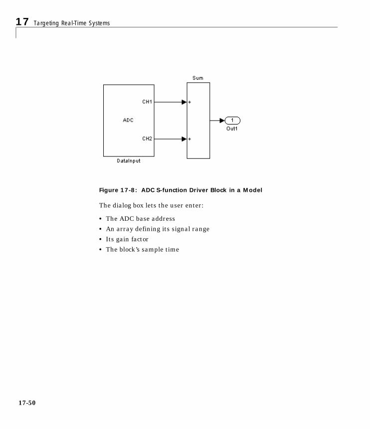
17 Targeting Real-Time Systems
17-50
Figure 17-8: ADC S-function Driver Block in a Model
The dialog box lets the user enter:
• The ADC base address
• An array defining its signal range
• Its gain factor
• The block’s sample time
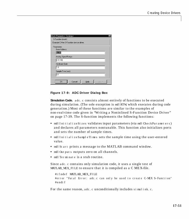
Creating Device Drivers
17-51
Figure 17-9: ADC Driver Dialog Box
Simulation Code. adc.c consists almost entirely of functions to be executedduring simulation. (The sole exception is mdlRTW, which executes during codegeneration.) Most of these functions are similar to the examples ofnon-real-time code given in “Writing a Noninlined S-Function Device Driver”on page 17-39. The S-function implements the following functions:
• mdlInitializeSizes validates input parameters (via mdlCheckParameters)and declares all parameters nontunable. This function also initializes portsand sets the number of sample times.
• mdlInitializeSampleTimes sets the sample time using the user-enteredvalue.
• mdlStart prints a message to the MATLAB command window.
• mdlOutputs outputs zero on all channels.
• mdlTerminate is a stub routine.
Since adc.c contains only simulation code, it uses a single test ofMATLAB_MEX_FILE to ensure that it is compiled as a C MEX-file.
#ifndef MATLAB_MEX_FILE#error "Fatal Error: adc.c can only be used to create C-MEX S-Function"#endif
For the same reason, adc.c unconditionally includes simulink.c.
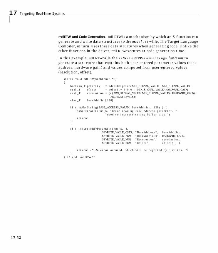
17 Targeting Real-Time Systems
17-52
mdlRTW and Code Generation. mdlRTW is a mechanism by which an S-function cangenerate and write data structures to the model.rtw file. The Target LanguageCompiler, in turn, uses these data structures when generating code. Unlike theother functions in the driver, mdlRTW executes at code generation time.
In this example, mdlRTW calls the ssWriteRTWParamSettings function togenerate a structure that contains both user-entered parameter values (baseaddress, hardware gain) and values computed from user-entered values(resolution, offset).
static void mdlRTW(SimStruct *S){ boolean_T polarity = adcIsUnipolar(MIN_SIGNAL_VALUE, MAX_SIGNAL_VALUE); real_T offset = polarity ? 0.0 : MIN_SIGNAL_VALUE/HARDWARE_GAIN; real_T resolution = (((MAX_SIGNAL_VALUE-MIN_SIGNAL_VALUE)/HARDWARE_GAIN)/ ADC_NUM_LEVELS); char_T baseAddrStr[128];
if ( mxGetString(BASE_ADDRESS_PARAM, baseAddrStr, 128) ) { ssSetErrorStatus(S, "Error reading Base Address parameter, " "need to increase string buffer size."); return; }
if ( !ssWriteRTWParamSettings(S, 4, SSWRITE_VALUE_QSTR, "BaseAddress", baseAddrStr, SSWRITE_VALUE_NUM, "HardwareGain", HARDWARE_GAIN, SSWRITE_VALUE_NUM, "Resolution", resolution, SSWRITE_VALUE_NUM, "Offset", offset) ) {
return; /* An error occured, which will be reported by Simulink. */ }} /* end: mdlRTW */

Creating Device Drivers
17-53
The structure defined in model.rtw is
SFcnParamSettings { BaseAddress "0x300" HardwareGain 1.0 Resolution 0.0048828125 Offset -10.0}
(The actual values of SFcnParamSettings derive from data entered by theuser.)
Values stored in the SFcnParamSettings structure are referenced indriver.tlc, as in the following assignment statement.
%assign baseAddr = SFcnParamSettings.BaseAddress
The Target Language Compiler uses variables such as baseAddr to generateparameters in real-time code files such as model.c and model.h. This isdiscussed in the next section.
The TLC File. adc.tlc contains three TLC functions. The BlockTypeSetup function generates the statement
#include "device.h"
in the model.h file. The other two functions, Start and Outputs, generate codewithin the MdlStart and MdlOutputs functions of model.c.
Statements in adc.tlc, and in the generated code, employ macros and symbolsdefined in device.h, and parameter values in the SFcnParamSettingsstructure. The following code uses the values from the SFcnParamSettingsstructure above to generate code containing constant values:
%assign baseAddr = SFcnParamSettings.BaseAddress%assign hwGain = SFcnParamSettings.HardwareGain...adcSetHardwareGain(%<baseAddr>, adcGetGainMask(%<hwGain>));
The TLC code above generates this statement in the MdlOutputs function ofmodel.c.
adcSetHardwareGain(0x300, adcGetGainMask(1.0));
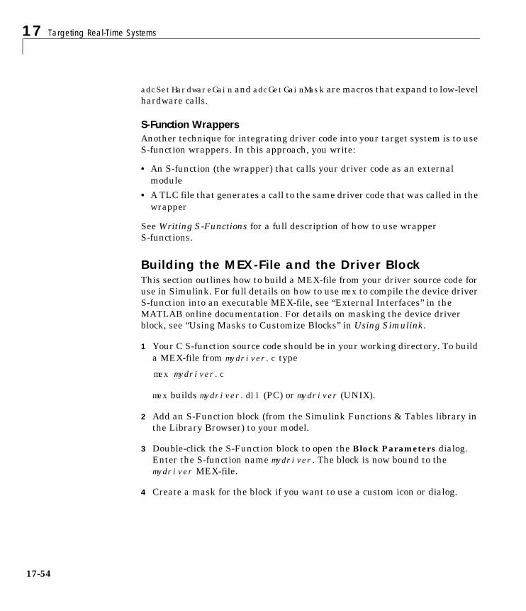
17 Targeting Real-Time Systems
17-54
adcSetHardwareGain and adcGetGainMask are macros that expand to low-levelhardware calls.
S-Function WrappersAnother technique for integrating driver code into your target system is to useS-function wrappers. In this approach, you write:
• An S-function (the wrapper) that calls your driver code as an externalmodule
• A TLC file that generates a call to the same driver code that was called in thewrapper
See Writing S-Functions for a full description of how to use wrapperS-functions.
Building the MEX-File and the Driver BlockThis section outlines how to build a MEX-file from your driver source code foruse in Simulink. For full details on how to use mex to compile the device driverS-function into an executable MEX-file, see “External Interfaces” in theMATLAB online documentation. For details on masking the device driverblock, see “Using Masks to Customize Blocks” in Using Simulink.
1 Your C S-function source code should be in your working directory. To builda MEX-file from mydriver.c type
mex mydriver.c
mex builds mydriver.dll (PC) or mydriver (UNIX).
2 Add an S-Function block (from the Simulink Functions & Tables library inthe Library Browser) to your model.
3 Double-click the S-Function block to open the Block Parameters dialog.Enter the S-function name mydriver. The block is now bound to themydriver MEX-file.
4 Create a mask for the block if you want to use a custom icon or dialog.
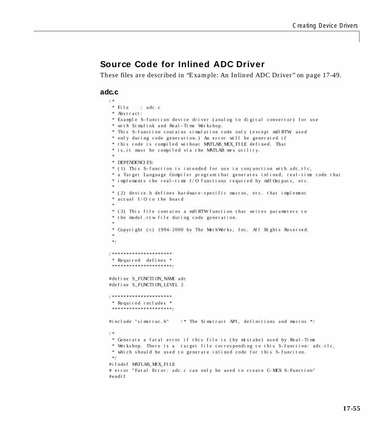
Creating Device Drivers
17-55
Source Code for Inlined ADC DriverThese files are described in “Example: An Inlined ADC Driver” on page 17-49.
adc.c/* * File : adc.c * Abstract: * Example S-function device driver (analog to digital convertor) for use * with Simulink and Real-Time Workshop. * This S-function contains simulation code only (except mdlRTW, used * only during code generation.) An error will be generated if * this code is compiled without MATLAB_MEX_FILE defined. That * is,it must be compiled via the MATLAB mex utility. * * DEPENDENCIES: * (1) This S-function is intended for use in conjunction with adc.tlc, * a Target Language Compiler program that generates inlined, real-time code that * implements the real-time I/O functions required by mdlOutputs, etc. * * (2) device.h defines hardware-specific macros, etc. that implement * actual I/O to the board * * (3) This file contains a mdlRTW function that writes parameters to * the model.rtw file during code generation. * * Copyright (c) 1994-2000 by The MathWorks, Inc. All Rights Reserved. * */
/********************* * Required defines * *********************/
#define S_FUNCTION_NAME adc#define S_FUNCTION_LEVEL 2
/********************* * Required includes * *********************/
#include "simstruc.h" /* The Simstruct API, definitions and macros */
/* * Generate a fatal error if this file is (by mistake) used by Real-Time * Workshop. There is a target file corresponding to this S-function: adc.tlc, * which should be used to generate inlined code for this S-funciton. */#ifndef MATLAB_MEX_FILE# error "Fatal Error: adc.c can only be used to create C-MEX S-Function"#endif
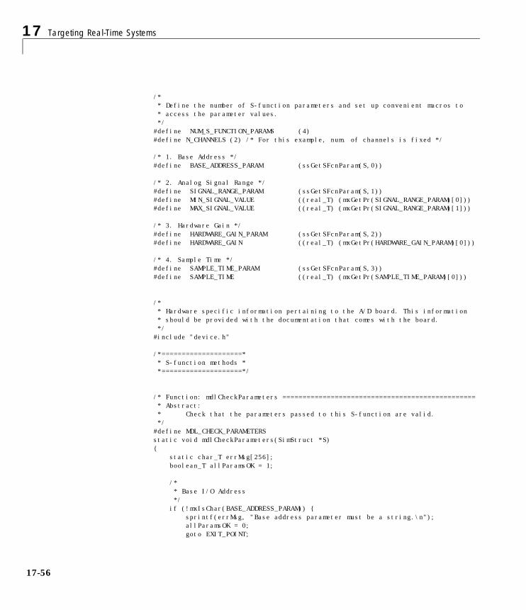
17 Targeting Real-Time Systems
17-56
/* * Define the number of S-function parameters and set up convenient macros to * access the parameter values. */#define NUM_S_FUNCTION_PARAMS (4)#define N_CHANNELS (2) /* For this example, num. of channels is fixed */
/* 1. Base Address */#define BASE_ADDRESS_PARAM (ssGetSFcnParam(S,0))
/* 2. Analog Signal Range */#define SIGNAL_RANGE_PARAM (ssGetSFcnParam(S,1))#define MIN_SIGNAL_VALUE ((real_T) (mxGetPr(SIGNAL_RANGE_PARAM)[0]))#define MAX_SIGNAL_VALUE ((real_T) (mxGetPr(SIGNAL_RANGE_PARAM)[1]))
/* 3. Hardware Gain */#define HARDWARE_GAIN_PARAM (ssGetSFcnParam(S,2))#define HARDWARE_GAIN ((real_T) (mxGetPr(HARDWARE_GAIN_PARAM)[0]))
/* 4. Sample Time */#define SAMPLE_TIME_PARAM (ssGetSFcnParam(S,3))#define SAMPLE_TIME ((real_T) (mxGetPr(SAMPLE_TIME_PARAM)[0]))
/* * Hardware specific information pertaining to the A/D board. This information * should be provided with the documentation that comes with the board. */#include "device.h"
/*====================* * S-function methods * *====================*/
/* Function: mdlCheckParameters ================================================ * Abstract: * Check that the parameters passed to this S-function are valid. */#define MDL_CHECK_PARAMETERSstatic void mdlCheckParameters(SimStruct *S){ static char_T errMsg[256]; boolean_T allParamsOK = 1;
/* * Base I/O Address */ if (!mxIsChar(BASE_ADDRESS_PARAM)) { sprintf(errMsg, "Base address parameter must be a string.\n"); allParamsOK = 0; goto EXIT_POINT;
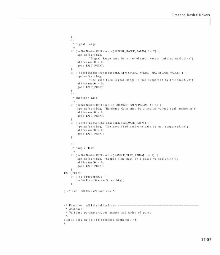
Creating Device Drivers
17-57
} /* * Signal Range */ if (mxGetNumberOfElements(SIGNAL_RANGE_PARAM) != 2) { sprintf(errMsg, "Signal Range must be a two element vector [minInp maxInp]\n"); allParamsOK = 0; goto EXIT_POINT; } if ( !adcIsSignalRangeParamOK(MIN_SIGNAL_VALUE, MAX_SIGNAL_VALUE) ) { sprintf(errMsg, "The specified Signal Range is not supported by I/O board.\n"); allParamsOK = 0; goto EXIT_POINT; } /* * Hardware Gain */ if (mxGetNumberOfElements(HARDWARE_GAIN_PARAM) != 1) { sprintf(errMsg, "Hardware Gain must be a scalar valued real number\n"); allParamsOK = 0; goto EXIT_POINT; } if (!adcIsHardwareGainParamOK(HARDWARE_GAIN)) { sprintf(errMsg, "The specified hardware gain is not supported.\n"); allParamsOK = 0; goto EXIT_POINT; } /* * Sample Time */ if (mxGetNumberOfElements(SAMPLE_TIME_PARAM) != 1) { sprintf(errMsg, "Sample Time must be a positive scalar.\n"); allParamsOK = 0; goto EXIT_POINT; }EXIT_POINT: if ( !allParamsOK ) { ssSetErrorStatus(S, errMsg); }
} /* end: mdlCheckParameters */
/* Function: mdlInitializeSizes ================================================ * Abstract: * Validate parameters,set number and width of ports. */static void mdlInitializeSizes(SimStruct *S){
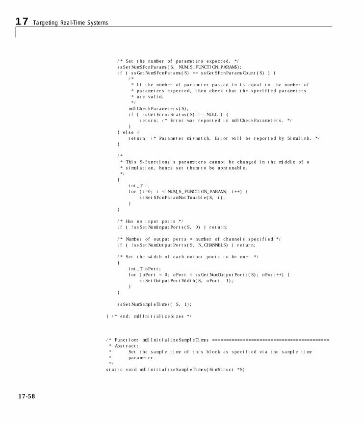
17 Targeting Real-Time Systems
17-58
/* Set the number of parameters expected. */ ssSetNumSFcnParams(S, NUM_S_FUNCTION_PARAMS); if ( ssGetNumSFcnParams(S) == ssGetSFcnParamsCount(S) ) { /* * If the number of parameter passed in is equal to the number of * parameters expected, then check that the specified parameters * are valid. */ mdlCheckParameters(S); if ( ssGetErrorStatus(S) != NULL ) { return; /* Error was reported in mdlCheckParameters. */ } } else { return; /* Parameter mismatch. Error will be reported by Simulink. */ }
/* * This S-functions's parameters cannot be changed in the middle of a * simulation, hence set them to be nontunable. */ { int_T i; for (i=0; i < NUM_S_FUNCTION_PARAMS; i++) { ssSetSFcnParamNotTunable(S, i); } }
/* Has no input ports */ if ( !ssSetNumInputPorts(S, 0) ) return;
/* Number of output ports = number of channels specified */ if ( !ssSetNumOutputPorts(S, N_CHANNELS) ) return;
/* Set the width of each output ports to be one. */ { int_T oPort; for (oPort = 0; oPort < ssGetNumOutputPorts(S); oPort++) { ssSetOutputPortWidth(S, oPort, 1); } }
ssSetNumSampleTimes( S, 1);
} /* end: mdlInitializeSizes */
/* Function: mdlInitializeSampleTimes ========================================== * Abstract: * Set the sample time of this block as specified via the sample time * parameter. */static void mdlInitializeSampleTimes(SimStruct *S)
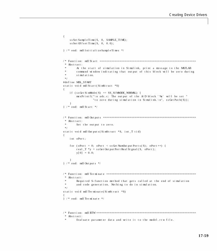
Creating Device Drivers
17-59
{ ssSetSampleTime(S, 0, SAMPLE_TIME); ssSetOffsetTime(S, 0, 0.0);
} /* end: mdlInitializeSampleTimes */
/* Function: mdlStart ========================================================== * Abstract: * At the start of simulation in Simulink, print a message to the MATLAB * command window indicating that output of this block will be zero during * simulation. */#define MDL_STARTstatic void mdlStart(SimStruct *S){ if (ssGetSimMode(S) == SS_SIMMODE_NORMAL) { mexPrintf("\n adc.c: The output of the A/D block '%s' will be set " "to zero during simulation in Simulink.\n", ssGetPath(S)); }} /* end: mdlStart */
/* Function: mdlOutputs ======================================================== * Abstract: * Set the output to zero. */static void mdlOutputs(SimStruct *S, int_T tid){ int oPort;
for (oPort = 0; oPort < ssGetNumOutputPorts(S); oPort++) { real_T *y = ssGetOutputPortRealSignal(S, oPort); y[0] = 0.0;
}} /* end: mdlOutputs */
/* Function: mdlTerminate ====================================================== * Abstract: * Required S-function method that gets called at the end of simulation * and code generation. Nothing to do in simulation. */static void mdlTerminate(SimStruct *S){} /* end: mdlTerminate */
/* Function: mdlRTW ============================================================ * Abstract: * Evaluate parameter data and write it to the model.rtw file.
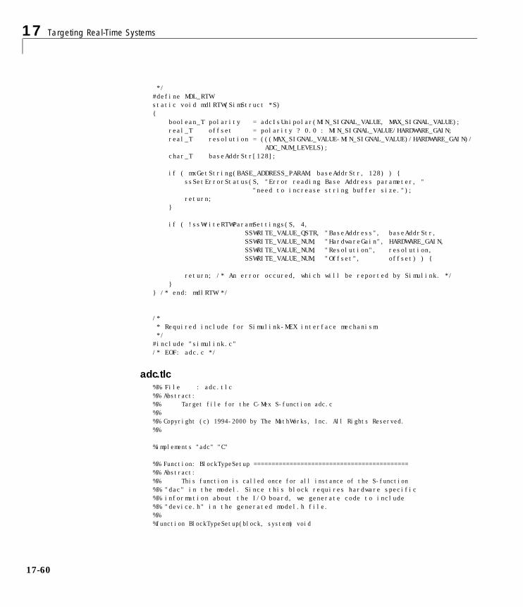
17 Targeting Real-Time Systems
17-60
*/#define MDL_RTWstatic void mdlRTW(SimStruct *S){ boolean_T polarity = adcIsUnipolar(MIN_SIGNAL_VALUE, MAX_SIGNAL_VALUE); real_T offset = polarity ? 0.0 : MIN_SIGNAL_VALUE/HARDWARE_GAIN; real_T resolution = (((MAX_SIGNAL_VALUE-MIN_SIGNAL_VALUE)/HARDWARE_GAIN)/ ADC_NUM_LEVELS); char_T baseAddrStr[128];
if ( mxGetString(BASE_ADDRESS_PARAM, baseAddrStr, 128) ) { ssSetErrorStatus(S, "Error reading Base Address parameter, " "need to increase string buffer size."); return; }
if ( !ssWriteRTWParamSettings(S, 4, SSWRITE_VALUE_QSTR, "BaseAddress", baseAddrStr, SSWRITE_VALUE_NUM, "HardwareGain", HARDWARE_GAIN, SSWRITE_VALUE_NUM, "Resolution", resolution, SSWRITE_VALUE_NUM, "Offset", offset) ) {
return; /* An error occured, which will be reported by Simulink. */ }} /* end: mdlRTW */
/* * Required include for Simulink-MEX interface mechanism */#include "simulink.c"/* EOF: adc.c */
adc.tlc%% File : adc.tlc%% Abstract:%% Target file for the C-Mex S-function adc.c%%%% Copyright (c) 1994-2000 by The MathWorks, Inc. All Rights Reserved.%%
%implements "adc" "C"
%% Function: BlockTypeSetup ===========================================%% Abstract:%% This function is called once for all instance of the S-function%% "dac" in the model. Since this block requires hardware specific%% information about the I/O board, we generate code to include%% "device.h" in the generated model.h file.%%%function BlockTypeSetup(block, system) void
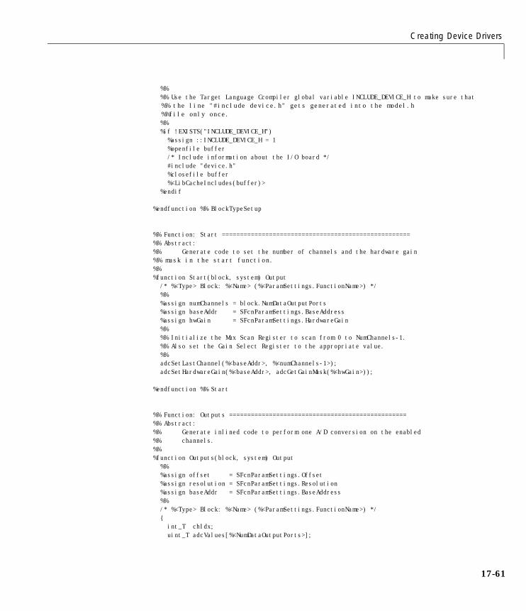
Creating Device Drivers
17-61
%% %% Use the Target Language Ccompiler global variable INCLUDE_DEVICE_H to make sure that
%% the line "#include device.h" gets generated into the model.h%%file only once.
%% %if !EXISTS("INCLUDE_DEVICE_H") %assign ::INCLUDE_DEVICE_H = 1 %openfile buffer /* Include information about the I/O board */ #include "device.h" %closefile buffer %<LibCacheIncludes(buffer)> %endif %endfunction %% BlockTypeSetup
%% Function: Start ====================================================%% Abstract:%% Generate code to set the number of channels and the hardware gain%% mask in the start function.%%%function Start(block, system) Output /* %<Type> Block: %<Name> (%<ParamSettings.FunctionName>) */ %% %assign numChannels = block.NumDataOutputPorts %assign baseAddr = SFcnParamSettings.BaseAddress %assign hwGain = SFcnParamSettings.HardwareGain %% %% Initialize the Mux Scan Register to scan from 0 to NumChannels-1. %% Also set the Gain Select Register to the appropriate value. %% adcSetLastChannel(%<baseAddr>, %<numChannels-1>); adcSetHardwareGain(%<baseAddr>, adcGetGainMask(%<hwGain>));
%endfunction %% Start
%% Function: Outputs =================================================%% Abstract:%% Generate inlined code to perform one A/D conversion on the enabled%% channels.%%%function Outputs(block, system) Output %% %assign offset = SFcnParamSettings.Offset %assign resolution = SFcnParamSettings.Resolution %assign baseAddr = SFcnParamSettings.BaseAddress %% /* %<Type> Block: %<Name> (%<ParamSettings.FunctionName>) */ { int_T chIdx; uint_T adcValues[%<NumDataOutputPorts>];
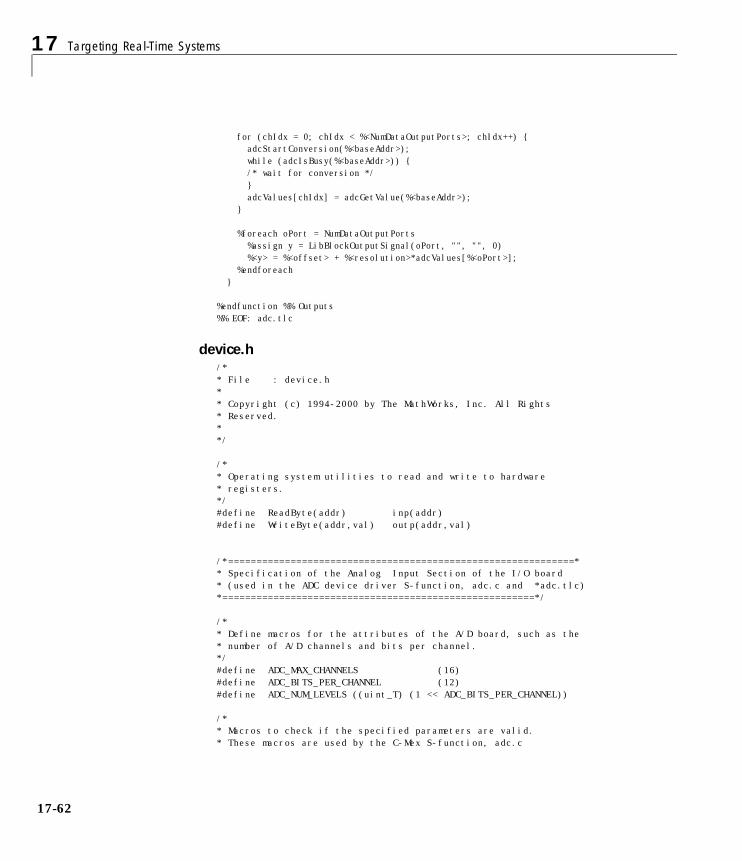
17 Targeting Real-Time Systems
17-62
for (chIdx = 0; chIdx < %<NumDataOutputPorts>; chIdx++) { adcStartConversion(%<baseAddr>); while (adcIsBusy(%<baseAddr>)) {
/* wait for conversion */ } adcValues[chIdx] = adcGetValue(%<baseAddr>); } %foreach oPort = NumDataOutputPorts %assign y = LibBlockOutputSignal(oPort, "", "", 0) %<y> = %<offset> + %<resolution>*adcValues[%<oPort>]; %endforeach }
%endfunction %% Outputs%% EOF: adc.tlc
device.h/** File : device.h** Copyright (c) 1994-2000 by The MathWorks, Inc. All Rights* Reserved.**/
/** Operating system utilities to read and write to hardware* registers.*/#define ReadByte(addr) inp(addr)#define WriteByte(addr,val) outp(addr,val)
/*=============================================================** Specification of the Analog Input Section of the I/O board* (used in the ADC device driver S-function, adc.c and *adc.tlc)*=======================================================*/
/** Define macros for the attributes of the A/D board, such as the* number of A/D channels and bits per channel.*/#define ADC_MAX_CHANNELS (16)#define ADC_BITS_PER_CHANNEL (12)#define ADC_NUM_LEVELS ((uint_T) (1 << ADC_BITS_PER_CHANNEL))
/** Macros to check if the specified parameters are valid.* These macros are used by the C-Mex S-function, adc.c
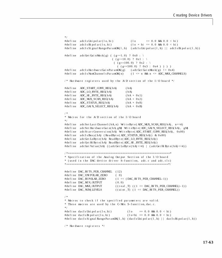
Creating Device Drivers
17-63
*/#define adcIsUnipolar(lo,hi) (lo == 0.0 && 0.0 < hi)#define adcIsBipolar(lo,hi) (lo + hi == 0.0 && 0.0 < hi)#define adcIsSignalRangeParamOK(l,h) (adcIsUnipolar(l,h) || adcIsBipolar(l,h))
#define adcGetGainMask(g) ( (g==1.0) ? 0x0 : \ ( (g==10.0) ? 0x1 : \ ( (g==100.0) ? 0x2 : \ ( (g==500.0) ? 0x3 : 0x4 ) ) ) )#define adcIsHardwareGainParamOK(g) (adcGetGainMask(g) != 0x4)#define adcIsNumChannelsParamOK(n) (1 <= n && n <= ADC_MAX_CHANNELS)
/* Hardware registers used by the A/D section of the I/O board */
#define ADC_START_CONV_REG(bA) (bA)#define ADC_LO_BYTE_REG(bA) (bA)#define ADC_HI_BYTE_REG(bA) (bA + 0x1)#define ADC_MUX_SCAN_REG(bA) (bA + 0x2)#define ADC_STATUS_REG(bA) (bA + 0x8)#define ADC_GAIN_SELECT_REG(bA) (bA + 0xB)
/** Macros for the A/D section of the I/O board*/#define adcSetLastChannel(bA,n) WriteByte(ADC_MUX_SCAN_REG(bA), n<<4)#define adcSetHardwareGain(bA,gM) WriteByte(ADC_GAIN_SELECT_REG(bA), gM)#define adcStartConversion(bA) WriteByte(ADC_START_CONV_REG(bA), 0x00)#define adcIsBusy(bA) (ReadByte(ADC_STATUS_REG(bA)) & 0x80)#define adcGetLoByte(bA) ReadByte(ADC_LO_BYTE_REG(bA))#define adcGetHiByte(bA) ReadByte(ADC_HI_BYTE_REG(bA))#define adcGetValue(bA) ((adcGetLoByte(bA)>>4) | (adcGetHiByte(bA)<<4))
/*============================================================** Specification of the Analog Output Section of the I/O board* (used in the DAC device driver S-function, adc.c and adc.tlc)*============================================================*/
#define DAC_BITS_PER_CHANNEL (12)#define DAC_UNIPOLAR_ZERO ( 0)#define DAC_BIPOLAR_ZERO (1 << (DAC_BITS_PER_CHANNEL-1))#define DAC_MIN_OUTPUT (0.0)#define DAC_MAX_OUTPUT ((real_T) ((1 << DAC_BITS_PER_CHANNEL)-1))#define DAC_NUM_LEVELS ((uint_T) (1 << DAC_BITS_PER_CHANNEL))
/** Macros to check if the specified parameters are valid.* These macros are used by the C-Mex S-function,dac.c.*/#define dacIsUnipolar(lo,hi) (lo == 0.0 && 0.0 < hi)#define dacIsBipolar(lo,hi) (lo+hi == 0.0 && 0.0 < hi)#define dacIsSignalRangeParamOK(l,h) (dacIsUnipolar(l,h) || dacIsBipolar(l,h))
/* Hardware registers */
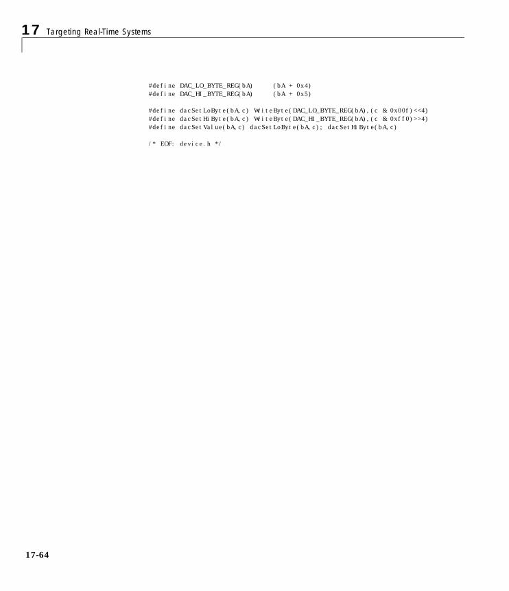
17 Targeting Real-Time Systems
17-64
#define DAC_LO_BYTE_REG(bA) (bA + 0x4)#define DAC_HI_BYTE_REG(bA) (bA + 0x5)
#define dacSetLoByte(bA,c) WriteByte(DAC_LO_BYTE_REG(bA),(c & 0x00f)<<4)#define dacSetHiByte(bA,c) WriteByte(DAC_HI_BYTE_REG(bA),(c & 0xff0)>>4)#define dacSetValue(bA,c) dacSetLoByte(bA,c); dacSetHiByte(bA,c)
/* EOF: device.h */
Interfacing Parameters and Signals
17-65
Interfacing Parameters and SignalsSimulink external mode (see Chapter 5, “External Mode”) offers a quick andeasy way to monitor signals and modify parameter values while generatedmodel code executes. However, external mode may not be appropriate for yourapplication. Some targets (such as the Real-Time Workshop Embedded Coder)do not support external mode, due to optimizations. In other cases, you maywant existing code to access parameters and signals of a model directly, ratherthan using the external mode mechanism.
The Real-Time Workshop supports several approaches to the task ofinterfacing block parameters and signals to your hand-written code.
The Workspace Parameter Attributes dialog enables you to declare how tothe generated code allocates memory for variables used in your model. Thisallows your supervisory software to read or write block parameter variables asyour model executes. Similarly, the Signal Properties dialog gives your codeaccess to selected signals within your model. Operation of these dialogs isdescribed in “Parameters: Storage, Interfacing, and Tuning” on page 3-51 and“Signals: Storage, Optimization, and Interfacing” on page 3-65.
In addition, the MathWorks provides C and Target Language Compiler APIsthat give your code additional access to block outputs, and parameters that arestored in global data structures created by the Real-Time Workshop. Thissection is an overview of these APIs. This section also includes pointers toadditional detailed API documents shipped with the Real-Time Workshop.
Signal Monitoring via Block OutputsAll block output data is written to the block outputs structure with each timestep in the model code. To access the output of a given block in the blockoutputs structure, your code must have the following information, per port:
• The address of the rtB structure where the data is stored
• The number of output ports of the block
• The width of each output
• The data type of the signal
This information is contained in the BlockIOSignals data structure. The TLCcode generation variable, BlockIOSignals, determines whether BlockIOSignals data is generated. If BlockIOSignals is enabled, a file

17 Targeting Real-Time Systems
17-66
containing an array of BlockIOSignals structures is written during codegeneration. This file is named model_bio.c.
BlockIOSignals is disabled by default. To enable generation of model_bio.c,use a %assign statement in the Configure RTW code generation settingssection of your system target file:
%assign BlockIOSignals = 1
Alternatively, you can append the following command to the System targetfile field on the Target configuration section of the Real-Time Workshoppage.
-aBlockIOSignals=1
Note that, depending on the size of your model, the BlockIOSignals array canconsume a considerable amount of memory.
BlockIOSignals and the Local Block Outputs OptionWhen the Local block outputs code generation option is selected, blockoutputs are declared locally in functions instead of being declared globally inthe rtB structure (when possible). The BlockIOSignals array in model_bio.c will not contain information about such locally declared signals. (Note thateven when all outputs in the system are declared locally, enablingBlockIOSignals will generate model_bio.c. In such a case theBlockIOSignals array will contain only a null entry.)
Signals that are designated as test points via the Signal Properties dialog aredeclared globally in the rtB structure, even when the Local block outputsoption is selected. Information about test-pointed signals is therefore writtento the BlockIOSignals array in model_bio.c.
Therefore, you can interface your code to selected signals by test-pointing themand enabling BlockIOSignals, without losing the benefits of the Local blockoutputs optimization for the other signals in your model.
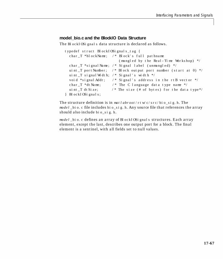
Interfacing Parameters and Signals
17-67
model_bio.c and the BlockIO Data StructureThe BlockIOSignals data structure is declared as follows.
typedef struct BlockIOSignals_tag {char_T *blockName; /* Block's full pathname
(mangled by the Real-Time Workshop) */char_T *signalName; /* Signal label (unmangled) */uint_T portNumber; /* Block output port number (start at 0) */uint_T signalWidth; /* Signal's width */void *signalAddr; /* Signal's address in the rtB vector */char_T *dtName; /* The C language data type name */uint_T dtSize; /* The size (# of bytes) for the data type*/
} BlockIOSignals;
The structure definition is in matlabroot/rtw/c/src/bio_sig.h. Themodel_bio.c file includes bio_sig.h. Any source file that references the arrayshould also include bio_sig.h.
model_bio.c defines an array of BlockIOSignals structures. Each arrayelement, except the last, describes one output port for a block. The finalelement is a sentinel, with all fields set to null values.
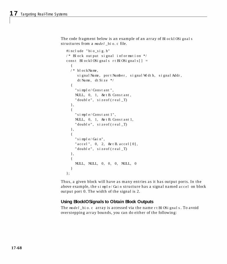
17 Targeting Real-Time Systems
17-68
The code fragment below is an example of an array of BlockIOSignals structures from a model_bio.c file.
#include "bio_sig.h"/* Block output signal information */const BlockIOSignals rtBIOSignals[] = { /* blockName, signalName, portNumber, signalWidth, signalAddr, dtName, dtSize */ { "simple/Constant", NULL, 0, 1, &rtB.Constant, "double", sizeof(real_T) }, { "simple/Constant1", NULL, 0, 1, &rtB.Constant1, "double", sizeof(real_T) }, { "simple/Gain", "accel", 0, 2, &rtB.accel[0], "double", sizeof(real_T) }, { NULL, NULL, 0, 0, 0, NULL, 0 }};
Thus, a given block will have as many entries as it has output ports. In theabove example, the simple/Gain structure has a signal named accel on blockoutput port 0. The width of the signal is 2.
Using BlockIOSignals to Obtain Block OutputsThe model_bio.c array is accessed via the name rtBIOSignals. To avoidoverstepping array bounds, you can do either of the following:

Interfacing Parameters and Signals
17-69
• Use the SimStruct access macro ssGetNumBlockIO to determine the numberof elements in the array.
• Test for a null blockName to identify the last element.
You must then write code that iterates over the rtBIOSignals array andchooses the signals to be monitored based on the blockName and signalName orportNumber. How the signals are monitored is up to you. For example, youcould collect the signals at every time step. Alternatively, you could samplesignals asynchronously in a separate, lower priority task.
The following code example is drawn from the main program (rt_main.c) of theTornado target. The code illustrates how the StethoScope GraphicalMonitoring/Data Analysis Tool uses BlockIOSignals to collect signalinformation in Tornado targets. The following function, rtInstallRemoveSignals, selectively installs signals from theBlockIOSignals array into the StethoScope Tool by callingScopeInstallSignal. The main simulation task then collects signals by callingScopeCollectSignals.
static int_T rtInstallRemoveSignals(SimStruct *S,char_T *installStr, int_T fullNames, int_T install){ uint_T i, w; char_T *blockName; char_T name[1024]; extern BlockIOSignals rtBIOSignals[]; int_T ret = -1; if (installStr == NULL) { return -1; }
i = 0; while(rtBIOSignals[i].blockName != NULL) { BlockIOSignals *blockInfo = &rtBIOSignals[i++]; if (fullNames) { blockName = blockInfo->blockName; } else { blockName = strrchr(blockInfo->blockName, '/'); if (blockName == NULL) {
blockName = blockInfo->blockName;} else {blockName++;
} }
if ((*installStr) == '*') {
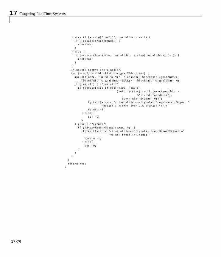
17 Targeting Real-Time Systems
17-70
} else if (strcmp("[A-Z]*", installStr) == 0) { if (!isupper(*blockName)) {
continue; } } else { if (strncmp(blockName, installStr, strlen(installStr)) != 0) {
continue; } } /*install/remove the signals*/ for (w = 0; w < blockInfo->signalWidth; w++) { sprintf(name, "%s_%d_%s_%d", blockName, blockInfo->portNumber,
(blockInfo->signalName==NULL)?"":blockInfo->signalName, w); if (install) { /*install*/
if (!ScopeInstallSignal(name, "units", (void *)((int)blockInfo->signalAddr +
w*blockInfo->dtSize), blockInfo->dtName, 0)) { fprintf(stderr,"rtInstallRemoveSignals: ScopeInstallSignal " "possible error: over 256 signals.\n"); return -1; } else { ret =0; } } else { /*remove*/
if (!ScopeRemoveSignal(name, 0)) {ifprintf(stderr,"rtInstallRemoveSignals: ScopeRemoveSignal\n"
"%s not found.\n",name); return -1;
} else { ret =0; } } } } return ret;}
Interfacing Parameters and Signals
17-71
Below is an excerpt from an example routine that collects signals taken fromthe main simulation loop.
/******************************************** Step the model for the base sample time ********************************************/
MdlOutputs(FIRST_TID);
#ifdef MAT_FILEif (rt_UpdateTXYLogVars(S) != NULL) {fprintf(stderr,"rt_UpdateTXYLogVars() failed\n");return(1);
}#endif
#ifdef STETHOSCOPEScopeCollectSignals(0);
#endif MdlUpdate(FIRST_TID);<code continues ...>
See Chapter 12, “Targeting Tornado for Real-Time Applications” for moreinformation on using StethoScope.
Parameter Tuning via model_pt.cBy enabling the TLC variable ParameterTuning, you can generate a filecontaining data structures that enable a running program to access modelparameters without use of external mode. The file is named model_pt.c.
ParameterTuning is disabled by default. To enable generation of model_pt.c,use a %assign statement in your system target file.
%assign ParameterTuning = 1
Alternatively, you can append the following command to the System targetfile field on the Target configuration section of the Real-Time Workshoppage.
-aParameterTuning=1
17 Targeting Real-Time Systems
17-72
model_pt.c contains two parameter mapping structures containinginformation required for parameter tuning:
• The BlockTuning structure contains all the modifiable block parameters byblock name and parameter name.
• The VariableTuning structure contains all the modifiable workspacevariables that were specified in a Simulink parameter dialog box.
The structure and content of the model_pt.c file are documented inmatlabroot/rtw/c/src/pt_readme.txt. For example source code using theparameter tuning API, see matlabroot/rtw/c/src/pt_print.c.
Target Language Compiler API forSignals and ParametersThe Real-Time Workshop provides a TLC function library that lets you createa global data map record. The global data map record, when generated, isadded to the CompiledModel structure in the model.rtw file. The global datamap record is a database containing all information required for accessingmemory in the generated code, including:
• Signals (Block I/O)
• Parameters
• Data type work vectors (DWork)
• External inputs
• External outputs
Use of the global data map requires knowledge of the Target LanguageCompiler and of the structure of the model.rtw file. See the Target LanguageCompiler Reference Guide for information on these topics.
The TLC functions that are required to generate and access the global datamap record are contained in matlabroot/rtw/c/tlc/globalmaplib.tlc. Thecomments in the source code fully document the global data map structuresand the library functions.
Note The global data map structures and functions maybe modified and/orenhanced in future releases.
Creating an External Mode Communication Channel
17-73
Creating an External Mode Communication ChannelThis section provides information you will need in order to support externalmode on your custom target, using your own low-level communications layer.This information includes:
• An overview of the design and operation of external mode
• A description of external mode source files
• Guidelines for modifying the external mode source files and rebuilding theext_comm MEX-file
This section assumes that you are familiar with the execution of Real-TimeWorkshop programs, and with the basic operation of external mode. Thesetopics are described in Chapter 6, “Program Architecture” and Chapter 5,“External Mode.”
The Design of External ModeExternal mode communication between Simulink and a target system is basedon a client/server architecture. The client (Simulink) transmits messagesrequesting the server (target) to accept parameter changes or to upload signaldata. The server responds by executing the request.
A low-level transport layer handles physical transmission of messages. BothSimulink and the model code are independent of this layer. Both the transportlayer and code directly interfacing to the transport layer are isolated inseparate modules that format, transmit and receive messages and datapackets.
This design makes it possible for different targets to use different transportlayers. For example, the grt, grt_malloc, and Tornado targets support host/target communication via TCP/IP, whereas the xPC Target supports bothRS232 (serial) and TCP/IP communication.
The Real-Time Workshop provides full source code for both the client andserver-side external mode modules, as used by the grt, grt_malloc, andTornado targets. The main client-side module is ext_comm.c. The mainserver-side module is ext_svr.c.
These two modules call the TCP/IP transport layer. ext_transport.cimplements the client-side transport functions. ext_svr_transport.c
17 Targeting Real-Time Systems
17-74
contains the corresponding server-side functions. You can modify these files tosupport external mode via your own low-level communications layer.
You need only modify those parts of the code that implement low-levelcommunications. You need not be concerned with issues such as dataconversions between host and target, or with the formatting of messages. Codeprovided by the Real-Time Workshop handles these functions.
On the client (Simulink) side, communications are handled by ext_comm, a CMEX-file. This component is implemented as a DLL on Windows, or as ashared library on UNIX.
On the server (target) side, external mode modules are linked into the targetexecutable. This takes place automatically if the External mode codegeneration option is selected at code generation time. These modules, calledfrom the main program and the model execution engine, are independent of thegenerated model code.
To implement your own low-level protocol:
• On the client side, you must replace low-level TCP/IP calls inext_transport.c with your own communication calls, and rebuild ext_commusing the mex command. You should then designate your custom ext_commcomponent as the MEX-file for external interface in the Simulink ExternalTarget Interface dialog.
• On the server side, you must replace low-level TCP/IP calls inext_svr_transport.cwith your own communication calls. If you are writingyour own system target file and/or template makefile, make sure that theEXT_MODE code generation option is defined. The generated makefile will thenlink ext_svr_transport.c and other server code into your executable.
• Define symbols and functions common to both the client and server sides inext_transport_share.h.
Overview of External Mode CommunicationsThis section gives a high-level overview of how a Real-Time Workshopgenerated program communicates with Simulink in external mode. Thisdescription is based on the TCP/IP version of external mode that ships withReal-Time Workshop.
Creating an External Mode Communication Channel
17-75
For communication to take place:
• The server (target) program must have been built with the conditionalEXT_MODE defined. EXT_MODE is defined in the model.mk file if the Externalmode code generation option was selected at code generation time.
• Both the server program and Simulink must be executing. Note that thisdoes not mean that the model code in the server system must be executing.The server may be waiting for Simulink to issue a command to start modelexecution.
The client and server communicate via two sockets. Each socket supports adistinct channel. The message channel is bidirectional; it carries commands,responses, and parameter downloads. The unidirectional upload channel is foruploading signal data to the client. The message channel is given higherpriority.
If the target program was invoked with the -w command line option, theprogram enters a wait state until it receives a message from the host.Otherwise, the program begins execution of the model. While the targetprogram is in a wait state, Simulink can download parameters to the targetand configure data uploading.
When the user chooses the Connect to target option from the Simulationmenu, the host initiates a handshake by sending an EXT_CONNECT message. Theserver responds with information about itself. This information includes:
• Checksums. The host uses model checksums to determine that the targetcode is an exact representation of the current Simulink model.
• Data format information. The host uses this information when formattingdata to be downloaded, or interpreting data that has been uploaded.
At this point, host and server are connected. The server is either executing themodel or in the wait state. (In the latter case, the user can begin modelexecution by selecting Start real-time code from the Simulation menu.)
During model execution, the message server runs as a background task. Thistask receives and processes messages such as parameter downloads.
Data uploading comprises both foreground execution and background servicingof the upload channel. As the target computes model outputs, it also copiessignal values into data upload buffers. This occurs as part of the taskassociated with each task identifier (tid). Therefore, data collection occurs in
17 Targeting Real-Time Systems
17-76
the foreground. Transmission of the collected data, however, occurs as abackground task. The background task sends the data in the collection buffersto Simulink via the upload channel.
The host initiates most exchanges on the message channel. The target usuallysends a response confirming that it has received and processed the message.Examples of messages and commands are:
• Connection message / connection response
• Start target simulation / start response
• Parameter download / parameter download response
• Arm trigger for data uploading
• Terminate target simulation / target shutdown response
Model execution terminates when the model reaches its final time, when thehost sends a terminate command, or when a Stop Simulation block terminatesexecution. On termination, the server informs the host that model executionhas stopped, and shuts down both sockets. The host also shuts down its sockets,and exits external mode.
External Mode Source Files
Host (ext_comm) Source FilesThe source files for the ext_comm component are located in the directorymatlabroot/rtw/ext_mode:
• ext_comm.c
This file is the core of external mode communication. It acts as a relay stationbetween the target and Simulink. ext_comm.c communicates to Simulink viaa shared data structure, ExternalSim. It communicates to the target via callsto the transport layer.
Tasks carried out by ext_comm include establishment of a connection withthe target, downloading of parameters, and termination of the connectionwith the target.
• ext_transport.c
This file implements required transport layer functions. (Note thatext_transport.c includes ext_transport_share.h, which containsfunctions common to client and server sides.) The version of

Creating an External Mode Communication Channel
17-77
ext_transport.c shipped with the Real-Time Workshop uses TCP/IPfunctions including recv(), send(), and socket().
• ext_main.c
This file is a MEX-file wrapper for external mode. ext_main interfaces toSimulink via the standard mexFunction call. (See “External Interfaces” inthe MATLAB online documentation for information on mexFunction.)ext_main contains a function dispatcher, esGetAction, that sends requestsfrom Simulink to ext_comm.
• ext_convert.c
This file contains functions used for converting data from host to targetformats (and vice versa). Functions include byte-swapping (big to little-endian), conversion from non-IEEE floats to IEEE doubles, and otherconversions. These functions are called both by ext_comm.c and directly bySimulink (via function pointers).
Note You do not need to customize ext_convert in order to implement acustom transport layer. However, it may be necessary to customizeext_convert for the intended target. For example, if the target represents thefloat data type in Texas Instruments (TI) format, ext_convert must bemodified to perform a TI to IEEE conversion.
• extsim.h
This file defines the ExternalSim data structure and access macros. Thisstructure is used for communication between Simulink and ext_comm.c.
• extutil.h
This file contains only conditionals for compilation of the assert macro.
Target (Server) Source FilesThese files are part of the run-time interface and are linked into the model.exeexecutable. They are located in the directory matlabroot/rtw/c/src.
• ext_svr.c
ext_svr.c is analogous to ext_comm.c on the host, but generally isresponsible for more tasks. It acts as a relay station between the host and thegenerated code. Like ext_comm.c, ext_svr.c carries out tasks such as

17 Targeting Real-Time Systems
17-78
establishing and terminating connection with the host. ext_svr.c alsocontains the background task functions that either write downloadedparameters to the target model, or extract data from the target data buffersand send it back to the host.
The version of ext_svr.c shipped with the Real-Time Workshop uses TCP/IP functions including recv(), send(), and socket().
• ext_svr_transport.c
This file implements required transport layer functions. (Note thatext_svr_transport.c includes ext_transport_share.h, which containsfunctions common to client and server sides.) The version ofext_svr_transport.c shipped with the Real-Time Workshop uses TCP/IPfunctions including recv(), send(), and socket().
• updown.c
updown.c handles the details of interacting with the target model. Duringparameter downloads, updown.c does the work of installing the newparameters into the model’s parameter vector. For data uploading, updown.ccontains the functions that extract data from the model’s blockio vector andwrite the data to the upload buffers. updown.c provides services both toext_svr.c and to the model code (e.g., grt_main.c). It contains code that iscalled via the background tasks of ext_svr.c as well as code that is called aspart of the higher priority model execution.
• dt_info.h and model.dt
These files contain data type transition information that allows access tomulti-data type structures across different computer architectures. Thisinformation is used in data conversions between host and target formats.
• updown_util.h
This file contains only conditionals for compilation of the assert macro.
Other Files
• ext_share.h
Contains message code definitions and other definitions required by both thehost and target modules.

Creating an External Mode Communication Channel
17-79
• ext_transport_share.h
Contains functions and data structures required by both the host and targetmodules of the transport layer. The version of ext_transport_share.hshipped with the Real-time Workshop is specific to TCP/IP communications.
Guidelines for Implementing the Transport Layer
Requirements
• ext_svr.c and updown.c use malloc to allocate buffers in target memory formessages, data collection, and other purposes. If your target uses some othermemory allocation scheme, you must modify these modules appropriately.
• The target is assumed to support both int32_T and uint32_T data types.
Guidelines for Modifying ext_transportThe function prototypes in ext_transport.h define the calling interface for thehost (client) side transport layer functions. The implementation is inext_transport.c.
To implement the host side of your transport layer:
• Replace the functions in the “Visible Functions” section of ext_transport.cwith functions that call your low-level communications primitives. Thevisible functions are called from other external mode modules such asext_comm.c. You must implement all the functions defined inext_transport.h. Your implementations must conform to the prototypesdefined in ext_transport.h.
• Supply a definition for the UserData structure in ext_transport.c. Thisstructure is required. If UserData is not necessary for your external modeimplementation, define a UserData structure with one dummy field.
• Replace the functions in ext_transport_share.h with functions that callyour low-level communications primitives, or remove these functions.Functions defined in ext_transport_share.h are common to the host andtarget, and are not part of the public interface to the transport layer.
• Rebuild the ext_comm MEX-file, using the MATLAB mex command. Thisrequires a compiler supported by the MATLAB API. See “ExternalInterfaces” in the MATLAB online documentation for more information on
17 Targeting Real-Time Systems
17-80
the mex command. The following table lists the form of the commands tobuild the standard ext_comm module on PC and UNIX platforms.
The ext_transport and ext_transport_share source code modules are fullycommented. See these files for further details.
Guidelines for Modifying ext_svr_transportThe function prototypes in ext_svr_transport.h define the calling interfacefor the target (server) side transport layer functions. The implementation is inext_svr_transport.c.
To implement the target side of your transport layer:
• Replace the functions in ext_svr_transport.c with functions that call yourlow-level communications primitives. These are the functions called fromother target modules such as the main program. You must implement all thefunctions defined in ext_svr_transport.h. Your implementations mustconform to the prototypes defined in ext_svr_transport.h.
• Supply a definition for the ExtUserData structure in ext_svr_transport.c.This structure is required. If ExtUserData is not necessary for your externalmode implementation, define an ExtUserData structure with one dummyfield.
• Define the EXT_BLOCKING conditional in ext_svr_transport.c as needed:
Table 17-4: Commands to Rebuild ext_comm MEX-Files
Platform Commands
PC cd matlabroot\toolbox\rtwmex matlabroot\rtw\ext_mode\ext_comm.c
matlabroot\rtw\ext_mode\ext_convert.c matlabroot\rtw\ext_mode\ext_transport.c–Imatlab\rtw\c\src –DWIN32 compiler_library_path\wsock32.lib
UNIX cd matlabroot/toolbox/rtwmex matlabroot/rtw/ext_mode/ext_comm.c
matlabroot/rtw/ext_mode/ext_convert.c matlabroot/rtw/ext_mode/ext_transport.c–Imatlab/rtw/c/src

Creating an External Mode Communication Channel
17-81
- Define EXT_BLOCKING as 0 to poll for a connection to the host (appropriatefor single-threaded applications).
- Define EXT_BLOCKING as 1 in multi-threaded applications where tasks areable to block for a connection to the host without blocking the entireprogram.
See also the comments on EXT_BLOCKING in ext_svr_transport.c.
The ext_svr_transport source code modules are fully commented. See thesefiles for further details.
17 Targeting Real-Time Systems
17-82
Combining Multiple ModelsIf you want to combine several models (or several instances of the same model)into a single executable, the Real-Time Workshop offers several options.
One solution is to use the S-function target to combine the models into a singlemodel, and then generate an executable using either the grt or grt_malloc targets. Simulink and Real-Time workshop implicitly handle connectionsbetween models, sequencing of calls to the models, and multiple sample rates.This is the simplest solution in many cases. See Chapter 10, “The S-FunctionTarget” for further information.
A second option, for embedded systems development, is to generate code fromyour models using the Real-Time Workshop Embedded Coder target. You caninterface the model code to a common harness program by directly calling theentry points to each model. The Real-Time Workshop Embedded Coder targethas certain restrictions that may not be appropriate for your application. Formore information, see “Requirements and Restrictions” in Chapter 9,“Real-Time Workshop Embedded Coder.”
The grt_malloc target is a third solution. It is appropriate in situations whereyou want do any or all of the following:
• Selectively control calls to more than one model.
• Use dynamic memory allocation.
• Include models that employ continuous states.
• Log data to multiple files.
• Run one of the models in external mode.
This section discusses how to use the grt_malloc target to combine models intoa single program. Before reading this section, you should become familiar withmodel execution in Real-Time Workshop programs. (See Chapter 6, “ProgramArchitecture” and Chapter 7, “Models with Multiple Sample Rates.”) It will behelpful to refer to grt_malloc_main.c while reading these chapters.
The procedure for building a multiple-model executable is fairlystraightforward. The first step is to generate and compile code from each of themodels that are to be combined. Next, the makefiles for each of the models arecombined into one makefile for creating the final multimodel executable. Thenext step is create a combined simulation engine by modifyinggrt_malloc_main.c to initialize and call the models correctly. Finally, the
Combining Multiple Models
17-83
combination makefile links the object files from the models and the mainprogram into an executable. “Example Mutliple-Model Program” on page 17-83discusses an example implementation.
Sharing Data Across ModelsWe recommend using unidirectional signal connections between models. Thisaffects the order in which models are called. For example, if an output signalfrom modelA is used as input to modelB, modelA’s output computation shouldbe called first.
Timing IssuesWe recommend that you generate all the models you are combining with thesame solver mode (either all singletasking or all multitasking.) In addition, ifthe models employ continuous states, the same solver should be used for allmodels.
If all the models to be combined have the same sample rates and the samenumber of rates, the models can share the same timing engine data structure.(The TimingData structure is defined in matlabroot/rtw/c/src/mrt_sim.c).Alternatively, the models can maintain separate timing engine datastructures, as in the example program discussed below.
If the models have the same base rate, but have different sub-rates, each modelshould maintain a separate timing engine data structure. Each model shoulduse the same base rate timer interrupt.
If the base rates for the models are not the same, the main program (such asgrt_malloc_main) must set up the timer interrupt to occur at the greatestcommon divisor rate of the models. The main program is responsible for callingeach of the models at the appropriate time interval.
Data Logging and External Mode SupportA multiple-model program can log data to separate MAT-files for each model(as in the example program discussed below.)
Only one of the models in a multiple-model program can use external mode.
Example Mutliple-Model ProgramAn example multiple-model program, distributed with Real-Time Workshop, islocated at matlabroot/rtw/c/grt_malloc/demos. This example combines two
17 Targeting Real-Time Systems
17-84
models, fuelsys1 and mcolon. Both models have the same base rate and thesame number of sample times. For simplicity, each model creates andmaintains a separate timing engine data structure (although it would bepossible for them to share a common structure.) Each model logs states,outputs, and simulation time to a separate model.mat file.
The example files consist of:
• The models, fuelsys1.mdl and mcolon.mdl
• Run-time interface components: modified main program(combine_malloc_main.c) and modified solver (ode5combine.c)
• Control files: modified model.bat and model.mk files
Runtime Interface Components. The main program, combine_malloc_main.c, is amodified version of grt_malloc_main.c. combine_malloc_main employs two#defines for the models. MODEL1() and MODEL2() are macros that returnpointers to the Simstructs for fuelsys1 and mcolon, respectively. The coderefers to the models through these pointers throughout, as in the followingextract.
SimStruct *S1;SimStruct *S2;...
S1 = MODEL1();S2 = MODEL2();...
sfcnInitializeSizes(S1);sfcnInitializeSizes(S2);sfcnInitializeSampleTimes(S1);sfcnInitializeSampleTimes(S2);...
combine_malloc_main.c calls initialization, execution, and cleanup functionsonce for each model.
combine_malloc_main.c also uses the following #defines:
• NCSTATES1 and NCSTATES2 represent the number of continuous states in eachmodel.
• MATFILEA and MATFILEB represent the MAT-files logged by each model.
Combining Multiple Models
17-85
To see all modifications in the main program, compare grt_malloc_main.c tocombine_malloc_main.c.
The solver, ode5combine.c, is also modified to handle multiple models. TheUpdateContinuousStates function has been modified to obtain the number ofcontinuous states from each model’s Simstruct at runtime. Simstructs arepassed in by reference.
Control Files. combine.bat was created from the generated control files fuelsys1.bat and mcolon.bat. These were modified to invoke the makefile,combine.mk.
combine.mk combines parameters from the generated makefiles, fuelsys1.mkand mcolon.mk. Note the following modifications:
• combine.mk contains the model-specific defines MODEL1, MODEL2, NCSTATES1,and NCSTATES2. Note that these defines are included in the CPP_REQ_DEFINESlist.
• The SOLVER parameter specifies ode5combine.c.
• The REQ_SRCS list includes combine_malloc_main.c.
• Two rules have been added in order for make to locate source files in the buildsubdirectories, fuelsys1_grt_malloc_rtw and mcolon_grt_malloc_rtw.
Building the Example Program. To try the example:
1 use the build command to generate code and compile object files for thefuelsys1 and mcolon models.
2 Modify the MATLAB_ROOT and MATLAB_BIN path information in combine.mk asappropriate for your installation.
3 At the command prompt, type
combine.bat (on PC)
or
make -f combine.mk (on UNIX)
to build the combine executable.
17 Targeting Real-Time Systems
17-86
DSP Processor SupportThe Real-Time Workshop now supports target processors that have only oneregister size (e.g., 32-bit). This makes data type emulation of 8 and 16 bits onthe TCI_C30/C40 DSP and similar processors possible.
To support these processors:
• Add the command-DDSP32=1
to your template makefile.
• Add the statement%assign DSP32=1
to your system target file.

ABlocks That Depend onAbsolute Time

A Blocks That Depend on Absolute Time
A-2
Some Simulink blocks use the value of absolute time (i.e., the time from thebeginning of the program to the present time) to calculate their outputs. If youare designing a program that is intended to run indefinitely, then you cannotuse blocks that have a dependency on absolute time.
The problem arises when the value of time reaches the largest value that canbe represented by a double precision number. At that point, time is no longerincremented and the output of the block is no longer correct.
Note In addition to the blocks listed below, logging Time (in the WorkspaceI/O page of the Simulation Parameters dialog box) also requires absolutetime.
The following Simulink blocks depend on absolute time:
• Continuous Blocks
- Derivative
- Transport Delay
- Variable Transport Delay
• Discrete Blocks
- Discrete-Time Integrator (when used in triggered subsystems)
• Nonlinear Blocks
- Rate Limiter
• Sinks
- Scope
- To File
- To Workspace (only if logging to StructureWithTime format)
• Sources
- Chirp Signal
- Clock
- Digital Clock
- Discrete Pulse Generator
- From File

A-3
- From Workspace
- Pulse Generator
- Ramp
- Repeating Sequence
- Signal Generator
- SineWave
- Step
In addition to the Simulink block above:
• Blocks in other Blocksets may reference absolute time. Please refer to thedocumentation for the Blocksets that you use.
• Stateflow charts that use time are dependent on absolute time.

A Blocks That Depend on Absolute Time
A-4

B
Glossary
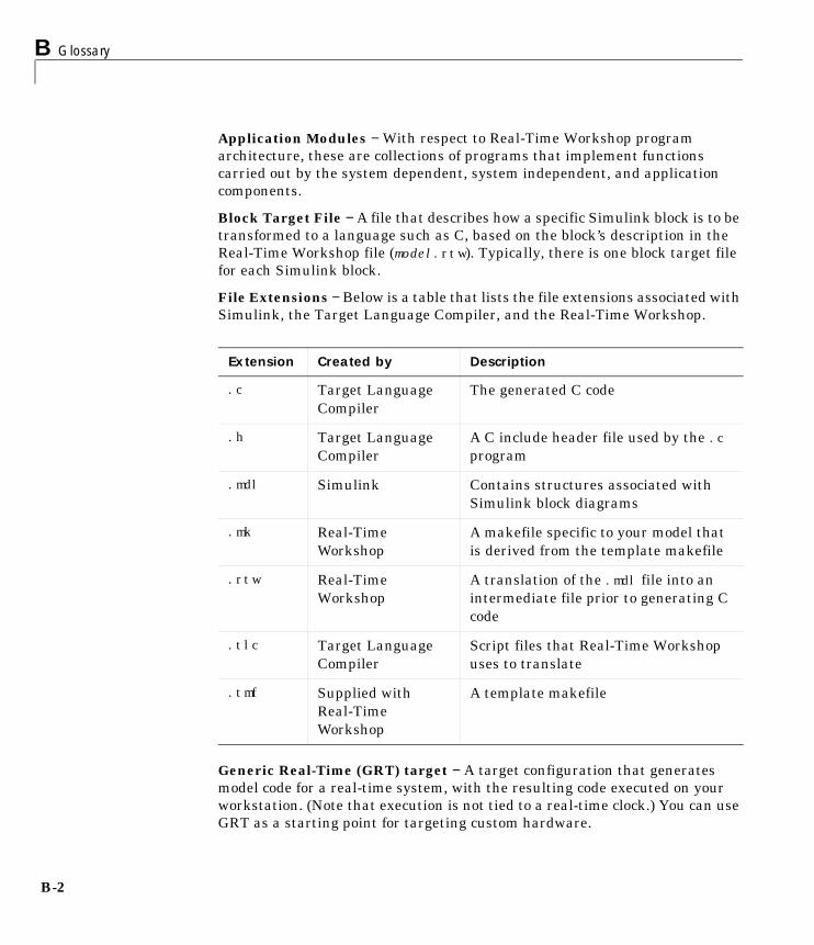
B Glossary
B-2
Application Modules − With respect to Real-Time Workshop programarchitecture, these are collections of programs that implement functionscarried out by the system dependent, system independent, and applicationcomponents.
Block Target File − A file that describes how a specific Simulink block is to betransformed to a language such as C, based on the block’s description in theReal-Time Workshop file (model.rtw). Typically, there is one block target filefor each Simulink block.
File Extensions − Below is a table that lists the file extensions associated withSimulink, the Target Language Compiler, and the Real-Time Workshop.
Generic Real-Time (GRT) target − A target configuration that generatesmodel code for a real-time system, with the resulting code executed on yourworkstation. (Note that execution is not tied to a real-time clock.) You can useGRT as a starting point for targeting custom hardware.
Extension Created by Description
.c Target LanguageCompiler
The generated C code
.h Target LanguageCompiler
A C include header file used by the .cprogram
.mdl Simulink Contains structures associated withSimulink block diagrams
.mk Real-TimeWorkshop
A makefile specific to your model thatis derived from the template makefile
.rtw Real-TimeWorkshop
A translation of the .mdl file into anintermediate file prior to generating Ccode
.tlc Target LanguageCompiler
Script files that Real-Time Workshopuses to translate
.tmf Supplied withReal-TimeWorkshop
A template makefile
B-3
Host System − The computer system on which you create your real-timeapplication.
Inline − Generally, this means to place something directly in the generatedsource code. You can inline parameters and S-functions using the Real-TimeWorkshop.
Inlined Parameters (Target Language Compiler Boolean global variable:InlineParameters) − The numerical values of the block parameters are hardcoded into the generated code. Advantages include faster execution and lessmemory use, but you lose the ability to change the block parameter values atrun-time.
Inlined S-Function − An S-function can be inlined into the generated code byimplementing it as a .tlc file. The code for this S-function is placed in thegenerated model code itself. In contrast, noninlined S-functions require afunction call to S-function residing in an external MEX-file.
Interrupt Service Routine (ISR) − A piece of code that your processorexecutes when an external event, such as a timer, occurs.
Loop Rolling (Target Language Compiler global variable: RollThreshold) −Depending on the block's operation and the width of the input/output ports, thegenerated code uses a for statement (rolled code) instead of repeating identicallines of code (flat code) over the block width.
Make − A utility to maintain, update, and regenerate related programs andfiles. The commands to be executed are placed in a makefile.
Makefiles − Files that contain a collection of commands that allow groups ofprograms, object files, libraries, etc. to interact. Makefiles are executed by yourdevelopment system’s make utility.
Multitasking − A process by which your microprocessor schedules thehandling of multiple tasks. The number of tasks is equal to the number ofsample times in your model.
Noninlined S-Function − In the context of the Real-Time Workshop, this isany C MEX S-function that is not implemented using a customized .tlc file. Ifyou create an C MEX S-function as part of a Simulink model, it is by defaultnoninlined unless you write your own .tlc file that inlines it.
Non-Real-Time − A simulation environment of a block diagram provided forhigh-speed simulation of your model. Execution is not tied to a real-time clock.
B Glossary
B-4
Nonvirtual Block − Any block that performs some algorithm, such as a Gainblock.
Pseudomultitasking − In processors that do not offer multitasking support,you can perform pseudomultitasking by scheduling events on a fixedtime-sharing basis.
Real-Time System – A system that uses actual hardware to implementalgorithms, for example, digital signal processing or control applications.
Run-time Interface − A wrapper around the generated code that can be builtinto a stand-alone executable. The run-time interface consists of routines tomove the time forward, save logged variables at the appropriate time steps, etc.The run-time interface is responsible for managing the execution of thereal-time program created from your Simulink block diagram.
S-Function − A customized Simulink block written in C or M-code. C-codeS-functions can be inlined in the Real-Time Workshop.
Singletasking − A mode in which a model runs in one task.
System Target File − The entry point to the Target Language Compilerprogram, used to transform the Real-Time Workshop file into target specificcode.
Target Language Compiler − A compiler that compiles and executes systemand target files.
Target File − A file that is compiled and executed by the Target LanguageCompiler. A combination of these files describes how to transform theReal-Time Workshop file (model.rtw) into target-specific code.
Target System − The computer system on which you execute your real-timeapplication.
Targeting − The process of creating an executable for your target system.
Template Makefile − A line-for-line makefile used by a make utility. Thetemplate makefile is converted to a makefile by copying the contents of thetemplate makefile (usually system.tmf) to a makefile (usually system.mk)replacing tokens describing your model’s configuration.
Target Language Compiler Program − A set of TLC files that describe howto convert a model.rtw file into generated code.
B-5
Task Identifier (tid) − Each sample time in your model is assigned a taskidentifier (tid). The tid is passed to the model output and update routines todecide which portion of your model should be executed at a given time.
Virtual Block − A connection or graphical block, for example, a Mux block.

B Glossary
B-6
I-1
Index
AAda code format 17-18Ada Coder
applications of 16-3blocks supported by 16-21code validation 16-18compilers supported by 16-3data logging 16-13signal properties 16-16targets supported by 16-3
application modulesapplication-specific components 6-34definition of 6-24system-independent components 6-30
atomic subsystem 3-41automatic S-function generation 10-12
See also S-function target
BBlock reduction optimization 3-23block target file 2-14blocks
Asynchronous Buffer 15-16Asynchronous Interrupt 15-5depending on absolute time A-2device driver 17-34nonvirtual 2-18Rate Transition 15-18Scope 3-19S-Function 10-4, 17-34Task Synchronization 15-12To File 3-20To Workspace 3-19Unit Delay 7-13virtual 2-18Zero-Order Hold 7-12
Build button 3-5Build command 3-5build directory
contents of 1-49, 3-98naming convention 1-43, 3-98
build processand code generation 3-2overview 2-12steps in 2-13
Ccode format
Ada 17-18choosing 4-3definition of 1-37embedded C 4-11real-time 4-6real-time malloc 4-8S-function 4-10, 10-2
code generation 3-1and simulation parameters 3-17automatic 2-12from nonvirtual subsystems 3-41TLC variables for 17-18tutorial 1-56
code generation optionsadvanced 3-22Block reduction 3-23Boolean logic signals 3-24External mode 3-14Force generation of parameter comments 3-13general 3-9Inline invariant signals 3-12Inline parameters 3-22Local block outputs
Index
I-2
See also Signal storage reuseLoop rolling threshold 3-10MAT-file variable name modifier 3-14Retain .rtw file 3-15Show eliminated statements 3-9Signal storage reuse 3-28
See also Local block outputsSolver page 3-17target specific 3-13TLC debugging 3-15Verbose builds 3-11Workspace I/O page 3-18
code tracing 3-28code validation
in Ada Coder 16-18tutorial 1-52
combining modelsin RTW Embedded Coder target 17-82via grt_malloc target 17-82via S-function target 17-82
communicationexternal mode 5-2external mode API for 17-73
continuous states, integration of 6-29Custom Code library
Custom Subsystem Code sublibrary 14-9overview 14-2
custom target configurationcomponents of 17-4tutorial 17-9
Ddata logging 3-18
in Ada Coder 16-13in single- and multitasking models 3-20to MAT-files 1-49, 3-18
tutorial 1-49via Scope blocks 3-19
example 1-53via To File blocks 3-20via To Workspace blocks 3-19
data structures in generated codeblock I/O 6-21block parameters 6-21block states 6-21external inputs 6-21external outputs 6-21
device driver blocksbuilding 17-54creating custom 17-34DOS 13-10inlined 17-48
example 17-49mdlRTW function in 17-52requirements for 17-48when to inline 17-36
limitations of 17-37noninlined 17-39
conditional compilation of 17-40required defines and includes 17-41required functions 17-42
parameterizing 17-38requirements for 17-37S-function wrappers for 17-54VxWorks 12-14
directoriesbuild 1-42used in build process 3-98working 1-42
DOSAnalog Input (ADC) block parameters 13-12Analog Output (DAC) block parameters 13-13building programs 13-17

Index
I-3
device driver blocks 13-7, 13-10, 13-11adding to model 13-16
Digital Input block parameters 13-14Digital Output block parameters 13-15hardware requirements 13-6implementation overview 13-4interrupt service routine 7-3Keithley Metrabyte board I/O driver 13-10modifying program timing 13-8program timing 13-7sample rate limits 13-7software requirements 13-6system configuration 13-5
DOS Device Drivers library 13-2doslib block library 13-10
EEmbedded Coder. See RTW Embedded Coder
targetembedded target. See RTW Embedded Coder
targetEuler integration algorithm 6-29expressions
tunable 3-51in masked subsystems 3-62limitations on 3-61
ext_comm MEX-file 5-40external mode 5-2, 17-73
APIhost source files 17-76implementing transport layer 17-79target source files 17-77
architecture 5-37, 17-73blocks compatible with 5-32code generation option 17-28, 17-75command line options for target program 5-42
communications overview 17-74configuring to use sockets 12-7control panel 5-9, 5-11download mechanism 5-36error conditions 5-44ext_comm MEX-file 5-36, 5-40
optional arguments to 5-40rebuilding 17-80
host and target systems in 5-2limitations of 5-45Signal Viewing Subsystems in 5-32TCP implementation 5-38tutorial 5-4using with VxWorks 12-6
Ffiles
generated See generated files
Ggenerated code
operations performed by 6-30generated files 2-17
model (UNIX executable) 2-17model.c 2-17model.exe 2-17model.exe (PC executable) 2-17model.h 2-17model.mdl 2-17model.mk 2-17model.rtw 2-17model_export.h 2-17
generated s-functionstunable parameters in 10-10
generic real-time (GRT) target 1-38tutorial 1-42
Index
I-4
Hhost
and target 1-37in external mode 5-2
Iinstallation xxiinterrupt service routine
locking and unlocking 15-11under DOS 7-3, 13-5under VxWorks 7-3
Interrupt Templates library 15-5
Llibraries
DOS Device Drivers 13-2Interrupt Templates 15-5VxWorks support 12-3
Local block outputs option 3-12
Mmake command 17-29make utility 2-12make_rtw 1-39, 2-12, 3-8MAT-files
file naming convention 3-19loading 1-55logging data to 1-49, 3-18variable names in 3-19
MATLAB 1-9required for Real-Time Workshop xviii
mdlRTW function 17-52
model codecustomizing 14-9execution of 6-32operations performed by 6-32
model executionin real time 7-10in Simulink 7-10Simulink vs. real-time 7-9
Model Parameter Configuration dialogtunable parameters and 3-51using 3-57
model registration function 6-32multitasking
building program for 7-8enabling 7-8task identifiers in 7-5task priorities 7-5versus singletasking 7-3
Nnonvirtual blocks 2-18nonvirtual subsystems
atomic 3-41categories of 3-41conditionally executed 3-41modularity of code generated from 3-48
Ooperating system
tasking primitives 6-10, 6-11VxWorks 12-2

Index
I-5
Pparameters
interfacing 3-51storage declarations 3-51tunable 3-51, 3-77
priorityof sample rates 7-5of VxWorks tasks 12-10
program architecturedata logging functions 6-32embedded 6-35initialization functions 6-26, 6-32main function 6-26model execution 6-27, 6-28model execution functions 6-32program execution 6-14program termination 6-27program timing 6-13rapid prototyping 6-25real-time 6-25termination functions 6-32
pseudomultitasking 7-5
Rrapid prototyping 2-2
for control systems 2-6for digital signal processing 2-5overview of process 2-2
rapid simulation targetbatch simulations (Monte Carlo) 11-12command line options 11-5
real timeexecuting models in 7-10integrating continuous states in 6-29
real-time malloc target 4-8combining models with 17-82
real-time object 9-4See also RTW Embedded Coder target
Real-Time Workshopopen architecture of 2-8user interface 3-4
Real-Time Workshop pageCategory menu 3-4opening 3-4overview 3-4Target configuration options 3-7
Browse button 3-7Build button 3-5Generate code only option 3-9Make command field 3-8System target file field 3-7Template makefile field 3-8
rsim. See rapid simulation targetRTW Embedded Coder target
automatic S-function wrapper generation 9-17code generation options 9-20, 9-27code generation report for 9-23code modules
generated 9-5header files 9-6main program 9-6user-written 9-8
data structureslogging object 9-4real-time object 9-4
inherent optimizations 9-2interfacing multiple models 9-16introduction to 9-2model entry points
calling directly 9-16modifying main program 9-10modifying rt_OneStep 9-14optimizing generated code 9-20

Index
I-6
program executionmain program 9-10rt_OneStep 9-11
multirate operation 9-12reentrancy 9-13single-rate operation 9-11
servicing timer interrupts 9-9requirements 9-29restrictions 9-29stack space allocation in 9-25system target files 9-31template makefiles 9-31unsupported blocks 9-30
run-time interface modules 1-60
Ssample rate transitions 7-12
faster to slowerin real-time 7-14in Simulink 7-13
slower to fasterin real-time 7-17in Simulink 7-16
sample time overlaps 7-17S-function target 4-10, 10-2
applications of 10-2automatic S-function generation 10-12generating reusable components with 10-4intellectual property protection in 10-3restrictions 10-15tunable parameters in 10-10unsupported blocks 10-16
S-functionsAPI 6-33generating automaticallymodels containing 6-32noninlined 6-32
signal properties 3-77setting via Signal Properties dialog 3-77
Signal storage reuse option 3-28Signal Viewing Subsystems 5-32simstruc.h
contents of 6-30SimStruct data structure
and global registration function 6-32definition of 6-30
Simulation Parameters dialogAdvanced page 3-22Diagnostics page 3-21Real-Time Workshop page 3-4Solver Options page 3-17Workspace I/O page 3-18
Simulink 1-9interactions with Real-Time Workshop 3-29
block execution order 3-32data propagation 3-29sample time propagation 3-31
required for Real-Time Workshop xviiisimulation parameters
and code generation 3-17Simulink data objects 3-79
and ObjectProperties records 3-88parameter objects 3-81signal objects 3-85
singletasking 7-9building program for 7-9enabling 7-9
step sizeof real-time continuous system 6-29
Index
I-7
StethoScopeSee VxWorks
subsystemnonvirtual 3-41
system records 2-18system target file 1-37, 2-14System Target File Browser 3-34, 3-36
Ttarget
available configurations 1-37bundled 1-22custom 1-23table of 3-36third-party 1-23
custom configuration 17-2DOS 13-2generic real-time See generic realtime (GRT)
targetrapid simulation See rapid simulation targetreal-time malloc See real-time malloc targetRTW Embedded Coder target. See RTW Em-
bedded Coder targetS-function See S-function targetTornado See VxWorks
Target Language Compilercode generation variables 17-18debugging options 3-15files
block target 1-38system target 1-38
function library 2-14generation of code by 2-14
task identifier (tid) 7-5, 9-12, 9-15template makefile 1-39
compiler-specific 3-102
default 3-99, 3-102defined 1-39options
Borland 3-105LCC 3-106UNIX 3-103Visual C/C++ 3-103, 3-104Watcom 3-105
structure of 17-25tokens 17-26
tid 9-12, 9-15tokens 17-26Tornado See VxWorkstutorials
building generic real-time program 1-42code generation 1-56code validation 1-52creating custom target configuration 17-9data logging 1-49external mode 5-4
Vvirtual blocks 2-18VxWorks 12-2
and external mode 12-6application overview 12-5configuring
for external mode (sockets) 12-6makefile template 12-14
connecting target to Ethernet 12-5downloading and running the executable inter-
actively 12-19external mode options 12-7GNU tools for 12-15implementation overview 12-12program build options 12-15
Index
I-8
program execution 12-20program monitoring 12-5real-time operating system 12-2runtime structure 12-8StethoScope code generation option 12-18support library 12-3target
connecting to 12-19downloading to 12-19
target CPU 12-5tasks created by 12-10template makefiles 12-14
Wworking directory 1-42