communications toolbox new features...
TRANSCRIPT

Computation
Visualization
Programming
For Use with MATLAB®
New Features GuideVersion 1.4 Release 11
CommunicationsToolbox
How to Contact The MathWorks:
508-647-7000 Phone
508-647-7001 Fax
The MathWorks, Inc. Mail24 Prime Park WayNatick, MA 01760-1500
http://www.mathworks.com Webftp.mathworks.com Anonymous FTP servercomp.soft-sys.matlab Newsgroup
[email protected] Technical [email protected] Product enhancement [email protected] Bug [email protected] Documentation error [email protected] Subscribing user [email protected] Order status, license renewals, [email protected] Sales, pricing, and general information
Communications Toolbox New Features Guide COPYRIGHT 1998-1999 by The MathWorks, Inc. All Rights Reserved.The software described in this document is furnished under a license agreement. The software may be usedor copied only under the terms of the license agreement. No part of this manual may be photocopied or repro-duced in any form without prior written consent from The MathWorks, Inc.
U.S. GOVERNMENT: If Licensee is acquiring the Programs on behalf of any unit or agency of the U.S.Government, the following shall apply: (a) For units of the Department of Defense: the Government shallhave only the rights specified in the license under which the commercial computer software or commercialsoftware documentation was obtained, as set forth in subparagraph (a) of the Rights in CommercialComputer Software or Commercial Software Documentation Clause at DFARS 227.7202-3, therefore therights set forth herein shall apply; and (b) For any other unit or agency: NOTICE: Notwithstanding anyother lease or license agreement that may pertain to, or accompany the delivery of, the computer softwareand accompanying documentation, the rights of the Government regarding its use, reproduction, and disclo-sure are as set forth in Clause 52.227-19 (c)(2) of the FAR.
MATLAB, Simulink, Stateflow, Handle Graphics, and Real-Time Workshop are registered trademarks, andTarget Language Compiler is a trademark of The MathWorks, Inc.
Other product or brand names are trademarks or registered trademarks of their respective holders.
Printing History: January 1998 First printing New for Version 1.3January 1999 Second printing Updated for Version 1.4 (Release 11)
☎PHONE
FAX
INTERNET
@

Contents
1New in the Communications Toolbox
Introduction . . . . . . . . . . . . . . . . . . . . . . . . . . . . . . . . . . . . . . . . . 1-2Requirements . . . . . . . . . . . . . . . . . . . . . . . . . . . . . . . . . . . . . . . . 1-2About This Document . . . . . . . . . . . . . . . . . . . . . . . . . . . . . . . . . 1-2Feedback . . . . . . . . . . . . . . . . . . . . . . . . . . . . . . . . . . . . . . . . . . . 1-2Accessing the Communications Toolbox Version 1.4 . . . . . . . . . 1-3Compatibility with Version 1.3 . . . . . . . . . . . . . . . . . . . . . . . . . . 1-3
What’s New in Version 1.4 . . . . . . . . . . . . . . . . . . . . . . . . . . . . . 1-4Reorganized and Streamlined Block Libraries . . . . . . . . . . . . . 1-4New Blocks . . . . . . . . . . . . . . . . . . . . . . . . . . . . . . . . . . . . . . . . . 1-10New Simulink Complex Data Type . . . . . . . . . . . . . . . . . . . . . 1-10Enhancements to Existing Blocks . . . . . . . . . . . . . . . . . . . . . . 1-10
2Using New Simulink Blocks
Introduction . . . . . . . . . . . . . . . . . . . . . . . . . . . . . . . . . . . . . . . . . 2-2
Gray Coded 8-PSK Modulation . . . . . . . . . . . . . . . . . . . . . . . . . 2-3Random Source Generation . . . . . . . . . . . . . . . . . . . . . . . . . . . . 2-5Gray Coded MPSK Modulation . . . . . . . . . . . . . . . . . . . . . . . . . 2-5Signal Transmission . . . . . . . . . . . . . . . . . . . . . . . . . . . . . . . . . . 2-8Gray Coded MPSK Demodulation . . . . . . . . . . . . . . . . . . . . . . . 2-9Symbol to Bit Conversion . . . . . . . . . . . . . . . . . . . . . . . . . . . . . 2-10Error Rate Calculation . . . . . . . . . . . . . . . . . . . . . . . . . . . . . . . 2-11Theoretical Performance . . . . . . . . . . . . . . . . . . . . . . . . . . . . . . 2-11Simulation Results . . . . . . . . . . . . . . . . . . . . . . . . . . . . . . . . . . 2-12
Punctured Convolutional Coding . . . . . . . . . . . . . . . . . . . . . 2-14Random Source Generation . . . . . . . . . . . . . . . . . . . . . . . . . . . 2-15Convolutional Encoding . . . . . . . . . . . . . . . . . . . . . . . . . . . . . . 2-16
i

ii Contents
Puncturing . . . . . . . . . . . . . . . . . . . . . . . . . . . . . . . . . . . . . . . . . 2-17Modulation . . . . . . . . . . . . . . . . . . . . . . . . . . . . . . . . . . . . . . . . . 2-18Signal Transmission . . . . . . . . . . . . . . . . . . . . . . . . . . . . . . . . . 2-18Demodulation . . . . . . . . . . . . . . . . . . . . . . . . . . . . . . . . . . . . . . . 2-19Erasure Insertion . . . . . . . . . . . . . . . . . . . . . . . . . . . . . . . . . . . . 2-19Viterbi Decoding . . . . . . . . . . . . . . . . . . . . . . . . . . . . . . . . . . . . . 2-20Error Rate Calculation . . . . . . . . . . . . . . . . . . . . . . . . . . . . . . . 2-20Stopping the Simulation . . . . . . . . . . . . . . . . . . . . . . . . . . . . . . 2-21Evaluating Results . . . . . . . . . . . . . . . . . . . . . . . . . . . . . . . . . . . 2-22Bibliography . . . . . . . . . . . . . . . . . . . . . . . . . . . . . . . . . . . . . . . . 2-24
3Simulink Block Library Reference
Overview . . . . . . . . . . . . . . . . . . . . . . . . . . . . . . . . . . . . . . . . . . . . . 3-2New Function Blocks in Version 1.4 . . . . . . . . . . . . . . . . . . . . . . 3-2AWGN Channel . . . . . . . . . . . . . . . . . . . . . . . . . . . . . . . . . . . . . . 3-3Block Interleave . . . . . . . . . . . . . . . . . . . . . . . . . . . . . . . . . . . . . . 3-6BPSK Demod . . . . . . . . . . . . . . . . . . . . . . . . . . . . . . . . . . . . . . . . 3-8BPSK Map . . . . . . . . . . . . . . . . . . . . . . . . . . . . . . . . . . . . . . . . . 3-10BPSK Mod . . . . . . . . . . . . . . . . . . . . . . . . . . . . . . . . . . . . . . . . . 3-11Convolutional Encoder . . . . . . . . . . . . . . . . . . . . . . . . . . . . . . . . 3-13Corr BPSK Demod . . . . . . . . . . . . . . . . . . . . . . . . . . . . . . . . . . . 3-17Data Mapper . . . . . . . . . . . . . . . . . . . . . . . . . . . . . . . . . . . . . . . 3-19Descrambler . . . . . . . . . . . . . . . . . . . . . . . . . . . . . . . . . . . . . . . . 3-22Differential Decoder . . . . . . . . . . . . . . . . . . . . . . . . . . . . . . . . . . 3-24Differential Encoder . . . . . . . . . . . . . . . . . . . . . . . . . . . . . . . . . . 3-25DPSK Demod . . . . . . . . . . . . . . . . . . . . . . . . . . . . . . . . . . . . . . . 3-26DPSK Mod . . . . . . . . . . . . . . . . . . . . . . . . . . . . . . . . . . . . . . . . . 3-28Error Rate Calculation . . . . . . . . . . . . . . . . . . . . . . . . . . . . . . . 3-30MSK Demod . . . . . . . . . . . . . . . . . . . . . . . . . . . . . . . . . . . . . . . . 3-32MSK Mod . . . . . . . . . . . . . . . . . . . . . . . . . . . . . . . . . . . . . . . . . . 3-34OQPSK Demap . . . . . . . . . . . . . . . . . . . . . . . . . . . . . . . . . . . . . . 3-36OQPSK Demod . . . . . . . . . . . . . . . . . . . . . . . . . . . . . . . . . . . . . . 3-37OQPSK Map . . . . . . . . . . . . . . . . . . . . . . . . . . . . . . . . . . . . . . . . 3-39OQPSK Mod . . . . . . . . . . . . . . . . . . . . . . . . . . . . . . . . . . . . . . . . 3-41PN Sequence . . . . . . . . . . . . . . . . . . . . . . . . . . . . . . . . . . . . . . . . 3-43
QPSK Demap . . . . . . . . . . . . . . . . . . . . . . . . . . . . . . . . . . . . . . . 3-45QPSK Demod . . . . . . . . . . . . . . . . . . . . . . . . . . . . . . . . . . . . . . . 3-46QPSK Map . . . . . . . . . . . . . . . . . . . . . . . . . . . . . . . . . . . . . . . . . 3-48QPSK Mod . . . . . . . . . . . . . . . . . . . . . . . . . . . . . . . . . . . . . . . . . 3-50Scrambler . . . . . . . . . . . . . . . . . . . . . . . . . . . . . . . . . . . . . . . . . . 3-52Viterbi Decoder . . . . . . . . . . . . . . . . . . . . . . . . . . . . . . . . . . . . . 3-54
ACorrections to User’s Guide
iii

iv Contents

Requirements . . . . . . . . . . . . . . . . . . . . 1-2About This Document . . . . . . . . . . . . . . . . . 1-2Feedback . . . . . . . . . . . . . . . . . . . . . . 1-2Accessing the Communications Toolbox Version 1.4 . . . . 1-3Compatibility with Version 1.3 . . . . . . . . . . . . . 1-3
What’s New in Version 1.4 . . . . . . . . . . . . . . 1-4Reorganized and Streamlined Block Libraries . . . . . . . 1-4New Blocks . . . . . . . . . . . . . . . . . . . . . 1-10New Simulink Complex Data Type . . . . . . . . . . . 1-10Enhancements to Existing Blocks . . . . . . . . . . . . 1-10
1
New in theCommunications ToolboxIntroduction . . . . . . . . . . . . . . . . . . . . 1-2
1 New in the Communications Toolbox
1-2
IntroductionVersion 1.4 (Release 11) is the newest release of the Communications Toolbox,a collection of MATLAB® functions and Simulink® blocks for research,development, system design, analysis, and simulation in the communicationsarea.
Note: This release does not include new MATLAB functions.
RequirementsThis release of the Communications Toolbox requires MATLAB Version 5.3.Simulink Version 3.0 and DSP Blockset Version 3.0 are required to use theSimulink blocks contained in the Communications Toolbox.
About This DocumentThis guide documents the functionality new to the Communications Toolbox,since Version 1.2. It also supplements the Communications Toolbox User’sGuide for Version 1.2, which is available online via the Help Desk, andsupersedes the Communications Toolbox New Features Guide Version 1.3.
This chapter provides an overview of new features and additions to theCommunications Toolbox for Version 1.4. Chapter 2 provides examples of howyou can use the new blocks. Chapter 3 describes all of the blocks added sinceVersion 1.2. Appendix A contains corrections to the Communications ToolboxUser’s Guide for Version 1.2.
FeedbackYour input is very valuable to us. Expanded functionality and improvementsto the Communications Toolbox are the result of your feedback. Please sendyour suggestions to: [email protected].
Introduction
Accessing the Communications Toolbox Version 1.4To access the Communications Toolbox from MATLAB, type the followingcommand.
commlib
The Communications Toolbox Library 1.4 (main library) window appears.
Compatibility with Version 1.3Some Communications Toolbox Version 1.4 blocks are not compatible withearlier versions. This results from a difference in how the Version 1.4 blockshandle complex signals. Simulink Version 3.0 and the CommunicationsToolbox Version 1.4 now support intrinsic complex data types. This means thatVersion 1.4 blocks handle complex inputs as single-width inputs, while earlierversion blocks require double-width inputs for complex signals. Therefore, youcannot use blocks from Communications Toolbox Version 1.4 libraries thathave complex inputs or outputs in models that you created with earlierversions of the Communications Toolbox.
You can continue to modify Version 1.3 models, since the CommunicationsToolbox Version 1.4 comes with both Version 1.4 and Version 1.3 blocklibraries. However, we recommend that you create new models using Version1.4 block libraries.
The Version 1.4 blocks that now process complex input signals as one signalinclude: baseband analog and digital modulation blocks, and channel blocks.
To access the Version 1.3 block libraries, type the following command in theMATLAB window.
commlib 1
The Communications Toolbox Simulink Block Library (the CommunicationsToolbox Version 1.3) window appears.
1-3

1 New in the Communications Toolbox
1-4
What’s New in Version 1.4The Communications Toolbox Version 1.4 contains the following changes andnew features:
• Reorganized and streamlined Simulink block libraries
• The following new Simulink blocks:
- Convolutional Encoder
- Viterbi Decoder
- Data Mapper
- Error Rate Calculation
• Support for the new Simulink complex data type
• Other Simulink block enhancements
Reorganized and Streamlined Block LibrariesThe Communications Toolbox Version 1.4 reorganizes and streamlines manyof the block libraries. This section describes the reorganization andstreamlining of the block libraries as follows:
• Table 1-1 lists the changes to the organization of the libraries from Version1.3 to Version 1.4.
• Figure 1-1 shows the block libraries and sublibraries for theCommunications Toolbox Version 1.4.
To display the Communications Toolbox Simulink Block library tree structurein the MATLAB window, type
help commlib
What’s New in Version 1.4
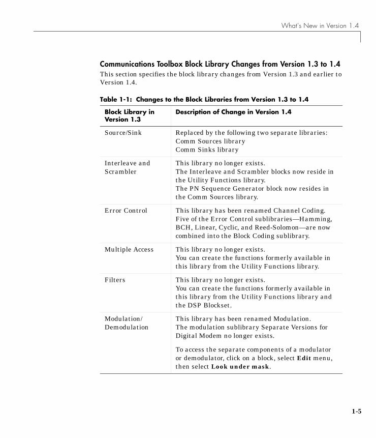
Communications Toolbox Block Library Changes from Version 1.3 to 1.4This section specifies the block library changes from Version 1.3 and earlier toVersion 1.4.
Table 1-1: Changes to the Block Libraries from Version 1.3 to 1.4
Block Library in Version 1.3
Description of Change in Version 1.4
Source/Sink Replaced by the following two separate libraries:Comm Sources libraryComm Sinks library
Interleave andScrambler
This library no longer exists.The Interleave and Scrambler blocks now reside inthe Utility Functions library.The PN Sequence Generator block now resides inthe Comm Sources library.
Error Control This library has been renamed Channel Coding.Five of the Error Control sublibraries—Hamming,BCH, Linear, Cyclic, and Reed-Solomon—are nowcombined into the Block Coding sublibrary.
Multiple Access This library no longer exists.You can create the functions formerly available inthis library from the Utility Functions library.
Filters This library no longer exists.You can create the functions formerly available inthis library from the Utility Functions library andthe DSP Blockset.
Modulation/Demodulation
This library has been renamed Modulation.The modulation sublibrary Separate Versions forDigital Modem no longer exists.
To access the separate components of a modulatoror demodulator, click on a block, select Edit menu,then select Look under mask.
1-5
1 New in the Communications Toolbox
1-6
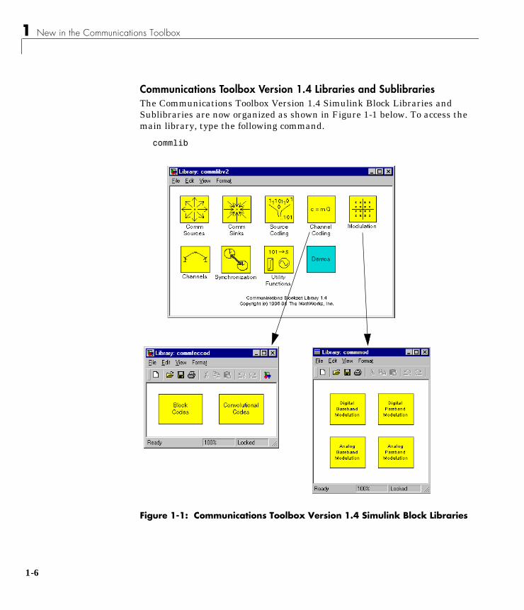
Communications Toolbox Version 1.4 Libraries and SublibrariesThe Communications Toolbox Version 1.4 Simulink Block Libraries andSublibraries are now organized as shown in Figure 1-1 below. To access themain library, type the following command.
commlib
Figure 1-1: Communications Toolbox Version 1.4 Simulink Block Libraries
What’s New in Version 1.4
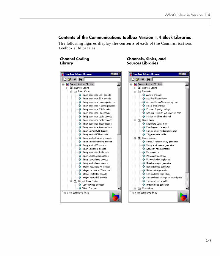
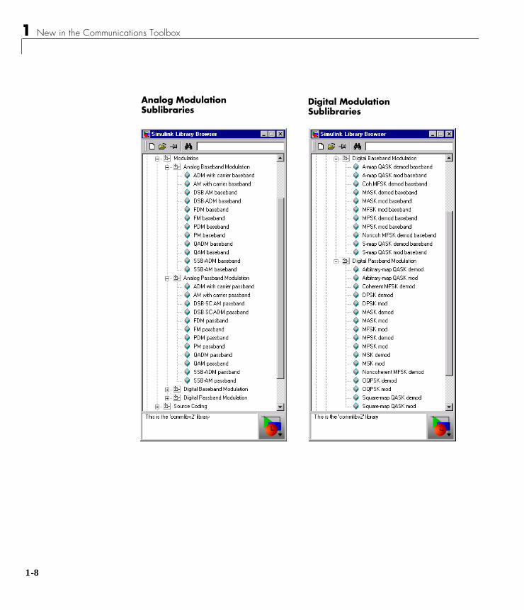
Contents of the Communications Toolbox Version 1.4 Block LibrariesThe following figures display the contents of each of the CommunicationsToolbox sublibraries.
Channel Coding Library
Channels, Sinks, and Sources Libraries
1-7
1 New in the Communications Toolbox
1-8
Digital Modulation Sublibraries
Analog Modulation Sublibraries
What’s New in Version 1.4
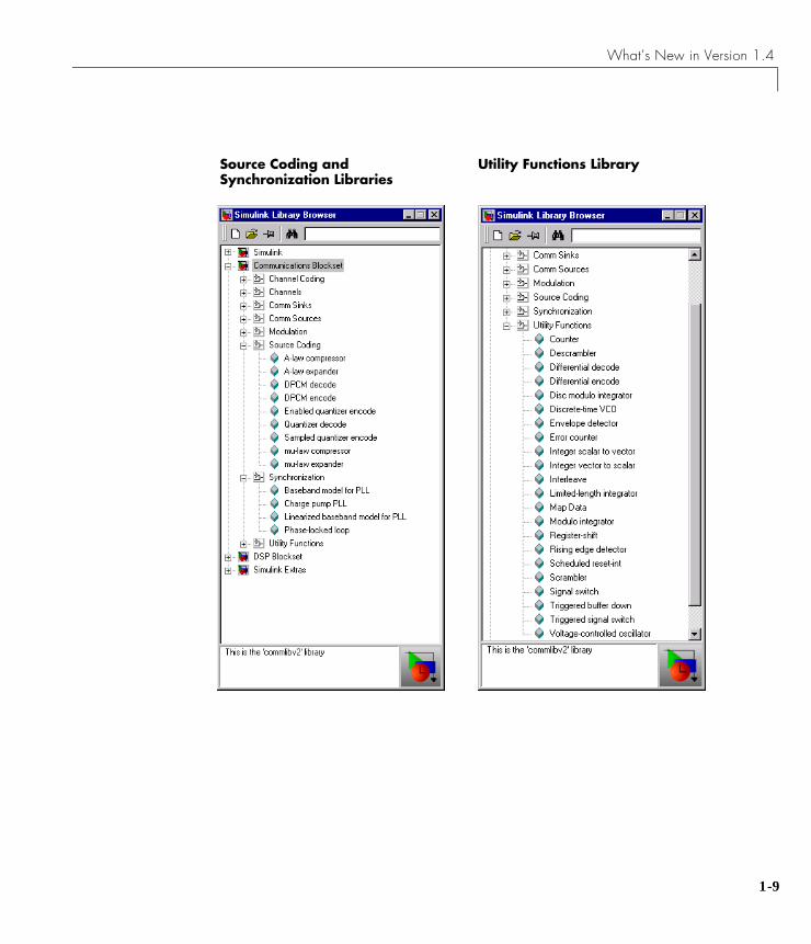
Source Coding and Synchronization Libraries
Utility Functions Library
1-9
1 New in the Communications Toolbox
1-1
New BlocksThe Communications Toolbox Version 1.4 contains the following new Simulinkblocks:
• Convolutional Encoder
• Viterbi Decoder
• Data Mapper
• Error Rate Calculation
Chapter 2 contains examples of how to use the new blocks. Chapter 3 containsreference pages, in alphabetical order, for each of the blocks added to theCommunications Toolbox since Version 1.2. See these reference pages fordetailed descriptions of how to use the new Simulink blocks.
New Simulink Complex Data TypeSimulink Version 3.0 now supports complex signals as an intrinsic data type.All of the Communications Toolbox Version 1.4 Simulink blocks that acceptcomplex signals as inputs or produce complex signals as outputs use this newdata type. See “Compatibility with Version 1.3” on page 1-3 for informationabout compatibility between Communications Toolbox Version 1.4 blocks andearlier versions.
Enhancements to Existing BlocksSome existing Simulink blocks in the Communications Toolbox have beenenhanced or modified in Version 1.4 as follows:
• You can now use the AWGN Channel block with either real or complexinputs. You can also supply the value of the noise variance either as a blockparameter or as an input to the block. With these two enhancements, thefunctionality of the AWGN Channel block now encompasses that of thefollowing four Version 1.3 blocks:
- The AWGN Channel block
- The AWGN w/ Varying Parameters block
- The Rayleigh Noise CE Channel block
- The Rayleigh Noise CE Channel w/ Varying Variance block
0
What’s New in Version 1.4
• You also now have the option to specify the noise variance in the parametermask for the AWGN Channel block in terms of the signal to noise ratio.
• You can choose to reverse the order of the vector elements in the IntegerScalar to Vector and Integer Vector to Scalar blocks.
• You can now set the modulation constant in the parameter mask for thefollowing eight phase and frequency modulation blocks:
- FDM Baseband
- FDM Passband
- FM Baseband
- FM Passband
- PDM Baseband
- PDM Passband
- PM Baseband
- PM Passband
In the FM (Frequency Modulator) and FDM (Frequency Demodulator)blocks, the modulation constant is specified in units of Hertz per volt. In thePM (Phase Modulator) and PDM (Phase Demodulator) blocks, themodulation constant is specified in units of radians per volt.
Both of the PDM blocks, Baseband and Passband, are implemented with aphase locked loop containing a voltage controlled oscillator (VCO). For thesetwo blocks you can also specify a value for the VCO gain in the parametermask, in units of Hertz per volt.
1-11

1 New in the Communications Toolbox
1-1
2
Gray Coded 8-PSK Modulation . . . . . . . . . . . 2-3Random Source Generation . . . . . . . . . . . . . . 2-5Gray Coded MPSK Modulation . . . . . . . . . . . . . 2-5Signal Transmission . . . . . . . . . . . . . . . . . 2-8Gray Coded MPSK Demodulation . . . . . . . . . . . . 2-9Symbol to Bit Conversion . . . . . . . . . . . . . . . 2-10Error Rate Calculation . . . . . . . . . . . . . . . . 2-11Theoretical Performance . . . . . . . . . . . . . . . . 2-11Simulation Results . . . . . . . . . . . . . . . . . . 2-12
Punctured Convolutional Coding . . . . . . . . . . 2-14Random Source Generation . . . . . . . . . . . . . . 2-15Convolutional Encoding . . . . . . . . . . . . . . . . 2-16Puncturing . . . . . . . . . . . . . . . . . . . . . 2-17Modulation . . . . . . . . . . . . . . . . . . . . . 2-18Signal Transmission . . . . . . . . . . . . . . . . . 2-18Demodulation . . . . . . . . . . . . . . . . . . . . 2-19Erasure Insertion . . . . . . . . . . . . . . . . . . 2-19Viterbi Decoding . . . . . . . . . . . . . . . . . . . 2-20Error Rate Calculation . . . . . . . . . . . . . . . . 2-20Stopping the Simulation . . . . . . . . . . . . . . . . 2-21Evaluating Results . . . . . . . . . . . . . . . . . . 2-22Bibliography . . . . . . . . . . . . . . . . . . . . 2-24
2
Using New SimulinkBlocksIntroduction . . . . . . . . . . . . . . . . . . . . 2-2

2 Using New Simulink Blocks
2-2
IntroductionThis chapter presents selected examples of the use of new Simulink blocksadded to the Communications Toolbox Version 1.4. Two examples illustrate theuse of the four new blocks as well as the modified AWGN Channel block.
The first example is a simulation of a communications link using 8-PSKmodulation with Gray coding. It includes the modified AWGN Channel blockand the new Data Mapper and Error Rate Calculation blocks.
The second example is a simulation of a coded communications link using apunctured convolutional code with Viterbi decoding. It includes the modifiedAWGN Channel block and the new Convolutional Encoder, Viterbi Decoder,and Error Rate Calculation blocks.

Gray Coded 8-PSK Modulation
Gray Coded 8-PSK ModulationGray coding is a technique often used in multilevel modulation schemesto minimize the bit error rate by ordering modulation symbols so that thebinary representations of adjacent symbols differ by only one bit. Thisexample shows how to use the new Data Mapper block to achieve thisordering.
The model shown below simulates the operation of a Gray coded 8-PSKmodulation system. To load this model from MATLAB, type
tstgraycod
Figure 2-1: Simulink Model of a Gray Coded 8-PSK Modulation System
2-3
2 Using New Simulink Blocks
2-4
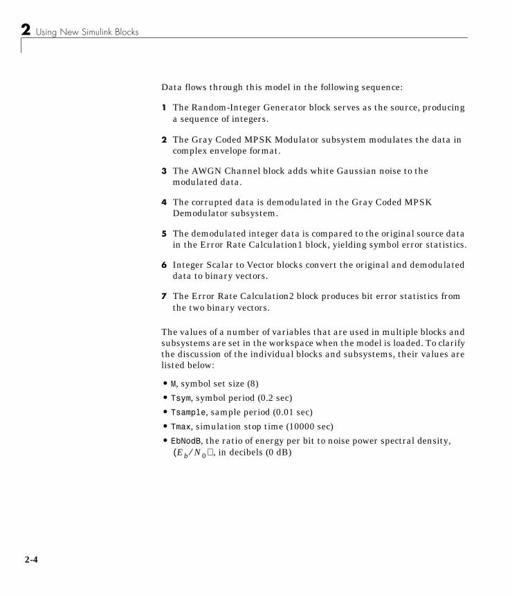
Data flows through this model in the following sequence:
1 The Random-Integer Generator block serves as the source, producinga sequence of integers.
2 The Gray Coded MPSK Modulator subsystem modulates the data incomplex envelope format.
3 The AWGN Channel block adds white Gaussian noise to themodulated data.
4 The corrupted data is demodulated in the Gray Coded MPSKDemodulator subsystem.
5 The demodulated integer data is compared to the original source datain the Error Rate Calculation1 block, yielding symbol error statistics.
6 Integer Scalar to Vector blocks convert the original and demodulateddata to binary vectors.
7 The Error Rate Calculation2 block produces bit error statistics fromthe two binary vectors.
The values of a number of variables that are used in multiple blocks andsubsystems are set in the workspace when the model is loaded. To clarifythe discussion of the individual blocks and subsystems, their values arelisted below:
• M, symbol set size (8)
• Tsym, symbol period (0.2 sec)
• Tsample, sample period (0.01 sec)
• Tmax, simulation stop time (10000 sec)
• EbNodB, the ratio of energy per bit to noise power spectral density,, in decibels (0 dB)Eb N0⁄( )

Gray Coded 8-PSK Modulation
Random Source GenerationThe Random Integer Generator block produces random data that is usedas the information in this simulation. Double-click on this block to openthe parameter mask window shown below.
This block generates one integer symbol in the range 0 to M-1 every Tsymseconds.
Gray Coded MPSK ModulationThe Gray Coded MPSK Modulation block, shown below, is a maskedsubsystem consisting of two Communications Toolbox library blocks inseries:
• The Data Mapper block
• The MPSK Mod Baseband block
2-5
2 Using New Simulink Blocks
2-6
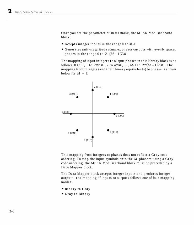
Once you set the parameter M in its mask, the MPSK Mod Basebandblock:
• Accepts integer inputs in the range 0 to M-1
• Generates unit-magnitude complex phasor outputs with evenly spacedphases in the range 0 to
The mapping of input integers to output phases in this library block is asfollows: 0 to , 1 to , 2 to , ... , M-1 to . Themapping from integers (and their binary equivalents) to phases is shownbelow for .
This mapping from integers to phases does not reflect a Gray codeordering. To map the input symbols onto the phasors using a Graycode ordering, the MPSK Mod Baseband block must be preceded by aData Mapper block.
The Data Mapper block accepts integer inputs and produces integeroutputs. The mapping of inputs to outputs follows one of four mappingmodes:
• Binary to Gray• Gray to Binary
2π M 1–( ) M⁄
0 2π M⁄ 4πM 2π M 1–( ) M⁄
M 8=
3 (011)
4 (100)0 (000)
7 (111)5 (101)
6 (110)
2 (010)
1 (001)
M
Gray Coded 8-PSK Modulation
• User Defined• Straight Through
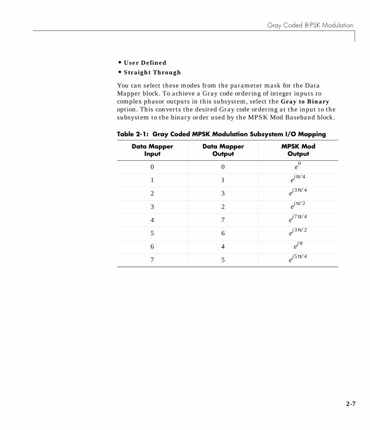
You can select these modes from the parameter mask for the DataMapper block. To achieve a Gray code ordering of integer inputs tocomplex phasor outputs in this subsystem, select the Gray to Binaryoption. This converts the desired Gray code ordering at the input to thesubsystem to the binary order used by the MPSK Mod Baseband block.
Table 2-1: Gray Coded MPSK Modulation Subsystem I/O Mapping
Data Mapper Input
Data Mapper Output
MPSK Mod Output
0 0
1 1
2 3
3 2
4 7
5 6
6 4
7 5
e0
ejπ 4⁄
ej3π 4⁄
ejπ 2⁄
ej7π 4⁄
ej3π 2⁄
ejπ
ej5π 4⁄
2-7
2 Using New Simulink Blocks
2-8
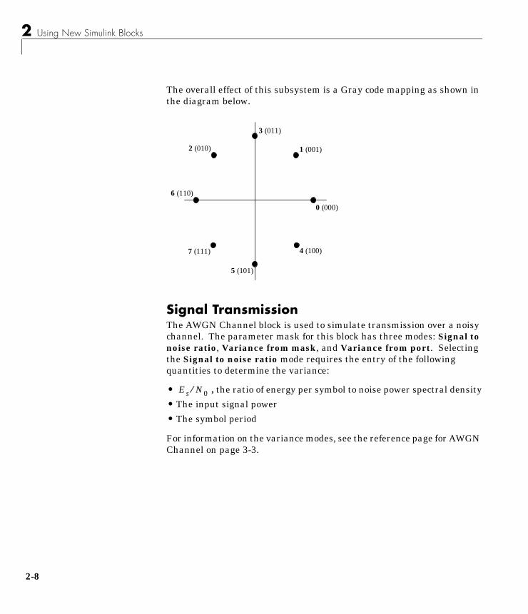
The overall effect of this subsystem is a Gray code mapping as shown inthe diagram below.
Signal TransmissionThe AWGN Channel block is used to simulate transmission over a noisychannel. The parameter mask for this block has three modes: Signal tonoise ratio, Variance from mask, and Variance from port. Selectingthe Signal to noise ratio mode requires the entry of the followingquantities to determine the variance:
• , the ratio of energy per symbol to noise power spectral density
• The input signal power
• The symbol period
For information on the variance modes, see the reference page for AWGNChannel on page 3-3.
2 (010)
6 (110)
0 (000)
4 (100)7 (111)
5 (101)
3 (011)
1 (001)
Es N0⁄

Gray Coded 8-PSK Modulation
The values for these parameters are chosen as follows:
• The parameter is computed from the workspace variablesEbNodB and M. The conversion from bit energy to symbol energy reflectsthe fact that each symbol carries log2(M) bits of information.
• The signal power is set to 1 watt because the M-PSK basebandmodulation block produces unit power signals.
• The symbol period of the channel is set to Tsym.
Gray Coded MPSK DemodulationTo construct the demodulation subsystem to correctly mirror the Graycoded modulation process:
• Follow the MPSK Demod Baseband block by a Data Mapper block asshown below.
• Set the mapping mode for the Data Mapper block to Binary to Gray inthe parameter mask.
Es N0⁄
2-9
2 Using New Simulink Blocks
2-1
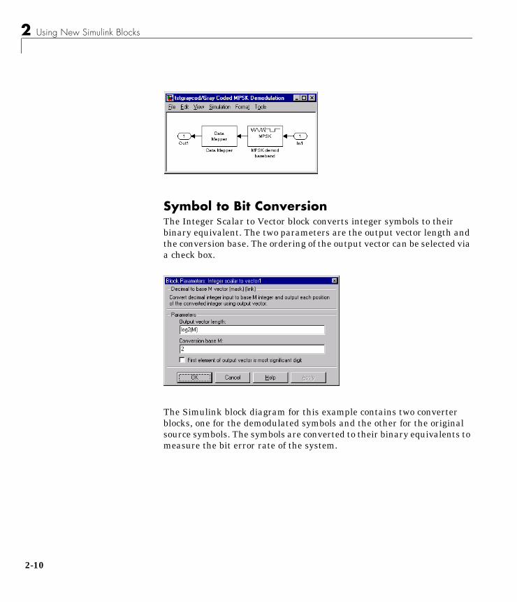
Symbol to Bit ConversionThe Integer Scalar to Vector block converts integer symbols to theirbinary equivalent. The two parameters are the output vector length andthe conversion base. The ordering of the output vector can be selected viaa check box.
The Simulink block diagram for this example contains two converterblocks, one for the demodulated symbols and the other for the originalsource symbols. The symbols are converted to their binary equivalents tomeasure the bit error rate of the system.
0
Gray Coded 8-PSK Modulation
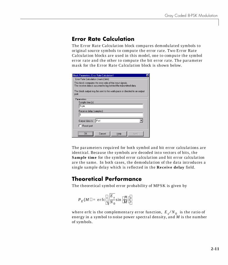
Error Rate CalculationThe Error Rate Calculation block compares demodulated symbols tooriginal source symbols to compute the error rate. Two Error RateCalculation blocks are used in this model, one to compute the symbolerror rate and the other to compute the bit error rate. The parametermask for the Error Rate Calculation block is shown below.
The parameters required for both symbol and bit error calculations areidentical. Because the symbols are decoded into vectors of bits, theSample time for the symbol error calculation and bit error calculationare the same. In both cases, the demodulation of the data introduces asingle sample delay which is reflected in the Receive delay field.
Theoretical PerformanceThe theoretical symbol error probability of MPSK is given by
where erfc is the complementary error function, is the ratio ofenergy in a symbol to noise power spectral density, and M is the numberof symbols.
PE M( ) erfcEsN0-------
πM-----
sin
=
Es N0⁄
2-11
2 Using New Simulink Blocks
2-1
To determine the bit error probability, the symbol error probability, ,needs to be converted to its bit error equivalent. There is no generalformula for the symbol to bit error conversion. Upper and lower limits arenevertheless easy to establish. The actual bit error probability, , canbe shown to be bounded by
The lower limit corresponds to the case where the symbols haveundergone Gray coding. The upper limit corresponds to the case wherepure binary coding is used.
Simulation ResultsTo test the Gray code modulation scheme in this model, simulate thetestmodmap model for a range of values. Because increasing thevalue of lowers the number of errors produced, the length ofeach simulation must be increased to ensure that the statistics of theerrors remain stable.
Using the sim command to run a Simulink simulation from MATLAB,the following code generates the data for symbol error rate and bit errorrate curves for values in the range 0 dB to 12 dB in steps of 2 dB.
M = 8;Tsym = 0.2;Tsample = 0.01;BERVec = [];SERVec = [];EbNoVec = [0:2:12];TVec = [1000 1000 1000 15000 20000 100000 100000]*Tsym;for n=1:length(EbNoVec); Tmax = TVec(n); EbNodB = EbNoVec(n); sim('testmodmap'); SERVec(n,:) = SER; BERVec(n,:) = BER;end;
PE
Pb
PE M( )M2log------------------ Pb
M 2⁄M 1–---------------PE M( )≤ ≤
Eb N0⁄Eb N0⁄
Eb N0⁄
2

Gray Coded 8-PSK Modulation
After simulating for the full set of values, you can plot thetheoretical and simulated results. These plots are shown in Figure 2-2.
Figure 2-2 also shows results for an 8-PSK modulation system withoutGray coding. To modify the model to generate this data, you must either:
• Replace the modulation and demodulation subsystems with the MPSKmodulator and demodulator blocks.
• Change the mode for each of the Data Mapper blocks in the modulationand demodulation subsystems to Straight Through.
Figure 2-2: Symbol and Bit Error Rates for 8-PSK
The simulation results agree well with the theoretical bounds for thesymbol and bit error probabilities. Since the Gray coding only affects themapping of symbol errors to bit errors, the symbol error probability is thesame in both cases.
Eb N0⁄
2-13
2 Using New Simulink Blocks
2-1
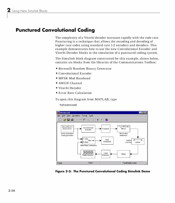
Punctured Convolutional CodingThe complexity of a Viterbi decoder increases rapidly with the code rate.Puncturing is a technique that allows the encoding and decoding ofhigher rate codes using standard rate 1/2 encoders and decoders. Thisexample demonstrates how to use the new Convolutional Encoder andViterbi Decoder blocks in the simulation of a punctured coding system.
The Simulink block diagram constructed for this example, shown below,contains six blocks from the libraries of the Communications Toolbox:
• Bernoulli Random Binary Generator
• Convolutional Encoder
• MPSK Mod Baseband
• AWGN Channel
• Viterbi Decoder
• Error Rate Calculation
To open this diagram from MATLAB, type
tstconvcod
Figure 2-3: The Punctured Convolutional Coding Simulink Demo
4
Punctured Convolutional Coding
Three additional subsystems have been constructed for the purpose ofthis example:
• The Puncture block periodically removes bits from the encoded bitstream, thereby increasing the code rate.
• The Insert Erasures block restores the encoded bit stream to theoriginal lower rate, allowing the use of a simpler decoder.
• The Stop Simulation block ends the simulation once a designatednumber of errors are observed or when a preset number of bits areprocessed.
Note: These three subsystems are presented as examples and are notpart of any library in the Communications Toolbox.
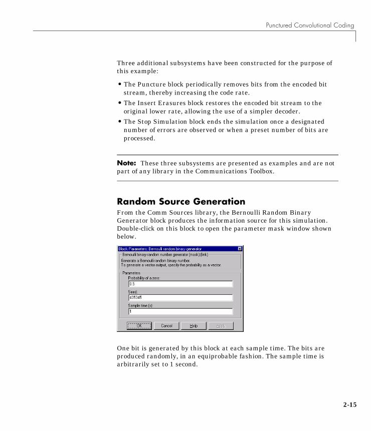
Random Source GenerationFrom the Comm Sources library, the Bernoulli Random BinaryGenerator block produces the information source for this simulation.Double-click on this block to open the parameter mask window shownbelow.
One bit is generated by this block at each sample time. The bits areproduced randomly, in an equiprobable fashion. The sample time isarbitrarily set to 1 second.
2-15
2 Using New Simulink Blocks
2-1
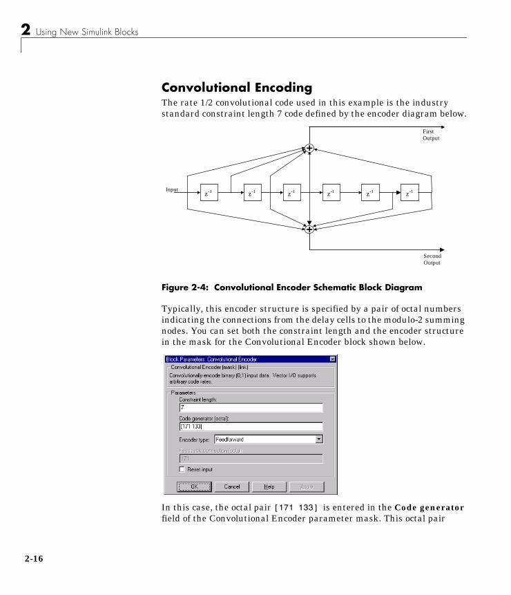
Convolutional EncodingThe rate 1/2 convolutional code used in this example is the industrystandard constraint length 7 code defined by the encoder diagram below.
Figure 2-4: Convolutional Encoder Schematic Block Diagram
Typically, this encoder structure is specified by a pair of octal numbersindicating the connections from the delay cells to the modulo-2 summingnodes. You can set both the constraint length and the encoder structurein the mask for the Convolutional Encoder block shown below.
In this case, the octal pair [171 133] is entered in the Code generatorfield of the Convolutional Encoder parameter mask. This octal pair
Input
FirstOutput
SecondOutput
z-1 z-1 z-1 z-1 z-1 z-1
6
Punctured Convolutional Coding
represents the shift register connections for the constraint length 7 codeshown in Figure 2-4.
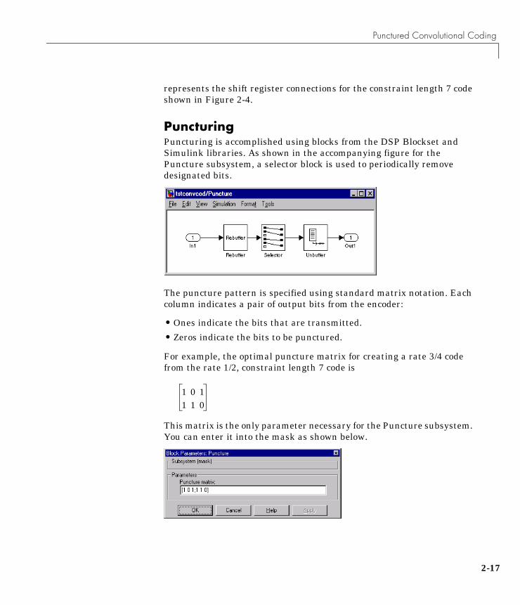
PuncturingPuncturing is accomplished using blocks from the DSP Blockset andSimulink libraries. As shown in the accompanying figure for thePuncture subsystem, a selector block is used to periodically removedesignated bits.
The puncture pattern is specified using standard matrix notation. Eachcolumn indicates a pair of output bits from the encoder:
• Ones indicate the bits that are transmitted.
• Zeros indicate the bits to be punctured.
For example, the optimal puncture matrix for creating a rate 3/4 codefrom the rate 1/2, constraint length 7 code is
This matrix is the only parameter necessary for the Puncture subsystem.You can enter it into the mask as shown below.
1 0 11 1 0
2-17
2 Using New Simulink Blocks
2-1
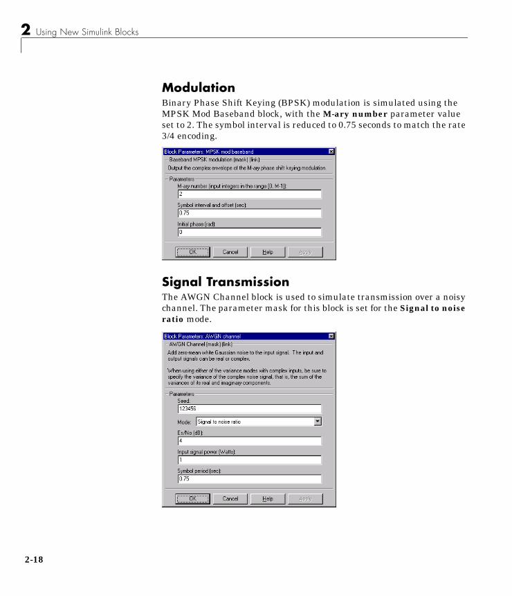
ModulationBinary Phase Shift Keying (BPSK) modulation is simulated using theMPSK Mod Baseband block, with the M-ary number parameter valueset to 2. The symbol interval is reduced to 0.75 seconds to match the rate3/4 encoding.
Signal TransmissionThe AWGN Channel block is used to simulate transmission over a noisychannel. The parameter mask for this block is set for the Signal to noiseratio mode.
8
Punctured Convolutional Coding
In this mask:
• The Es/No parameter is set to 4 dB in the mask parameters window.This value typically is changed from one simulation run to the next.
• The preceding modulation block generates unit power signals, so theInput signal power is set to 1 watt.
• The Symbol period is set to 0.75 seconds to match the symbol periodof the modulator.
DemodulationIn this simulation, the Viterbi Decoder block is set to accept unquantizedinputs. The MPSK Demodulator block produces hard decisions, so itcannot be used for demodulation in this model. Instead, the simulationpasses the channel output through a Simulink Complex to Real-Imagblock that extracts the real part of the complex samples.
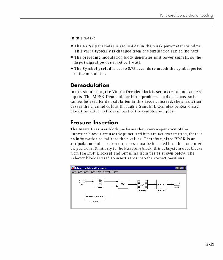
Erasure InsertionThe Insert Erasures block performs the inverse operation of thePuncture block. Because the punctured bits are not transmitted, there isno information to indicate their values. Therefore, since BPSK is anantipodal modulation format, zeros must be inserted into the puncturedbit positions. Similarly to the Puncture block, this subsystem uses blocksfrom the DSP Blockset and Simulink libraries as shown below. TheSelector block is used to insert zeros into the correct positions.
2-19

2 Using New Simulink Blocks
2-2
Viterbi DecodingThe Viterbi Decoder block is configured to decode the same rate 1/2 codespecified in the Convolutional Encoder block.
For this example, the decision type is set to Unquantized. You wouldnormally set the Traceback depth for this code to something close to 40.However, for decoding punctured codes, a higher value is required to givethe decoder time to resolve the ambiguities introduced by the insertederasures.
Error Rate CalculationThe decoded bits are compared to the original source bits in the ErrorRate Calculation block. In the mask for this block, shown below, thedecoder sample time is set to 1 second. The puncturing and erasureinsertion operations both introduce delay due to the use of buffers. Eachof these two blocks incurs 6 seconds of delay: 3 seconds each from the
0

Punctured Convolutional Coding
input and output buffers. Adding these delays to the decoder delay of 96seconds, produces a total Receive delay of 108 seconds.
Stopping the SimulationThe output of the Error Rate Calculation block is a three-element vectorcontaining the calculated bit error rate (BER), the number of errorsobserved, and the number of bits processed. BER simulations aretypically set to run until a minimum number of errors have beenobserved, or until a maximum number of bits have been processed.
You can use the Stop Simulation block to set these limits and to write thefinal BER data to the MATLAB workspace. To see how the StopSimulation block works:
• Select the Stop Simulation block.
• Select Look Under Mask in the Edit menu.
2-21
2 Using New Simulink Blocks
2-2
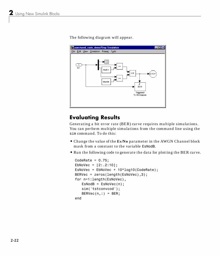
The following diagram will appear.
Evaluating ResultsGenerating a bit error rate (BER) curve requires multiple simulations.You can perform multiple simulations from the command line using thesim command. To do this:
• Change the value of the Es/No parameter in the AWGN Channel blockmask from a constant to the variable EsNodB.
• Run the following code to generate the data for plotting the BER curve.
CodeRate = 0.75;EbNoVec = [2:.2:10];EsNoVec = EbNoVec + 10*log10(CodeRate);BERVec = zeros(length(EsNoVec),3);for n=1:length(EsNoVec),
EsNodB = EsNoVec(n);sim('tstconvcod');BERVec(n,:) = BER;
end
2

Punctured Convolutional Coding
To confirm the validity of the results, we compare them to an establishedperformance bound. The bit error rate performance of a rate
punctured code is upper bounded by the expression
In this expression, erfc denotes the complementary error function, r isthe code rate, and both dfree and wd are dependent on the particular code.For the rate 3/4 code of this example, dfree = 5, w5 = 42, w6 = 201,w7 = 1492, and so on. See reference [1] for more details.
The following commands compute an approximation to this bound inMATLAB using the first seven terms of the summation:
dist = [5:11];nerr = [42 201 1492 10469 62935 379644 2253373];CodeRate = 3/4;EbNo_dB = [2:.02:10];EbNo = 10.0.^(EbNo_dB/10);arg = sqrt(CodeRate*ebno'*dist);bound = nerr*(1/6)*erfc(arg)';
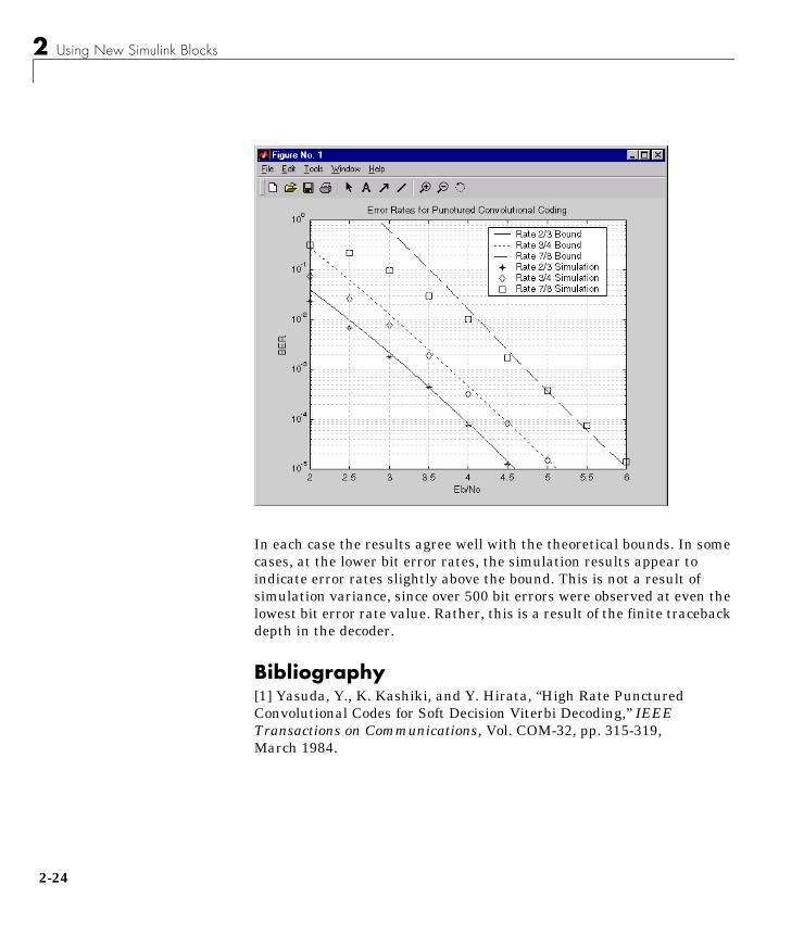
The figure below shows simulation results and bounds for the rate 3/4punctured code in this example, as well as other punctured codes of rates2/3 and 7/8 derived from the same original constraint length 7 rate 1/2code. The puncture patterns for these other rates are listed in reference[1]. The simulations used to generate the data for this plot were set tostop after 1000 errors or 40 million bits, whichever came first.
r n 1–( ) n⁄=
Pb1
2 n 1–( )--------------------- wderfc rd Eb N0⁄( )( )d dfree=
∞∑≤
2-23
2 Using New Simulink Blocks
2-2
In each case the results agree well with the theoretical bounds. In somecases, at the lower bit error rates, the simulation results appear toindicate error rates slightly above the bound. This is not a result ofsimulation variance, since over 500 bit errors were observed at even thelowest bit error rate value. Rather, this is a result of the finite tracebackdepth in the decoder.
Bibliography[1] Yasuda, Y., K. Kashiki, and Y. Hirata, “High Rate PuncturedConvolutional Codes for Soft Decision Viterbi Decoding,” IEEETransactions on Communications, Vol. COM-32, pp. 315-319,March 1984.
4
New Function Blocks in Version 1.4 . . . . . . . . . . . 3-2AWGN Channel . . . . . . . . . . . . . . . . . . . 3-3Block Interleave . . . . . . . . . . . . . . . . . . . 3-6BPSK Demod . . . . . . . . . . . . . . . . . . . . 3-8BPSK Map . . . . . . . . . . . . . . . . . . . . . 3-10BPSK Mod . . . . . . . . . . . . . . . . . . . . . 3-11Convolutional Encoder . . . . . . . . . . . . . . . . 3-13Corr BPSK Demod . . . . . . . . . . . . . . . . . . 3-17Data Mapper . . . . . . . . . . . . . . . . . . . . 3-19Descrambler . . . . . . . . . . . . . . . . . . . . 3-22Differential Decoder . . . . . . . . . . . . . . . . . 3-24Differential Encoder . . . . . . . . . . . . . . . . . 3-25DPSK Demod . . . . . . . . . . . . . . . . . . . . 3-26DPSK Mod . . . . . . . . . . . . . . . . . . . . . 3-28Error Rate Calculation . . . . . . . . . . . . . . . . 3-30MSK Demod . . . . . . . . . . . . . . . . . . . . 3-32MSK Mod . . . . . . . . . . . . . . . . . . . . . . 3-34OQPSK Demap . . . . . . . . . . . . . . . . . . . 3-36OQPSK Demod . . . . . . . . . . . . . . . . . . . 3-37OQPSK Map . . . . . . . . . . . . . . . . . . . . 3-39OQPSK Mod . . . . . . . . . . . . . . . . . . . . 3-41PN Sequence . . . . . . . . . . . . . . . . . . . . 3-43QPSK Demap . . . . . . . . . . . . . . . . . . . . 3-45QPSK Demod . . . . . . . . . . . . . . . . . . . . 3-46QPSK Map . . . . . . . . . . . . . . . . . . . . . 3-48QPSK Mod . . . . . . . . . . . . . . . . . . . . . 3-50Scrambler . . . . . . . . . . . . . . . . . . . . . 3-52Viterbi Decoder . . . . . . . . . . . . . . . . . . . 3-54
3
Simulink BlockLibrary ReferenceOverview . . . . . . . . . . . . . . . . . . . . . 3-2
3 Simulink Block Library Reference
3-2
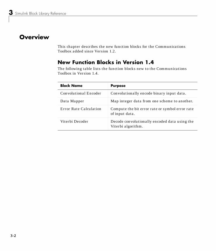
OverviewThis chapter describes the new function blocks for the CommunicationsToolbox added since Version 1.2.
New Function Blocks in Version 1.4The following table lists the function blocks new to the CommunicationsToolbox in Version 1.4.
Block Name Purpose
Convolutional Encoder Convolutionally encode binary input data.
Data Mapper Map integer data from one scheme to another.
Error Rate Calculation Compute the bit error rate or symbol error rateof input data.
Viterbi Decoder Decode convolutionally encoded data using theViterbi algorithm.

AWGN Channel
3AWGN ChannelPurpose Add zero-mean white Gaussian noise to the input signal.
Library Channels
Description You can use the AWGN Channel block with either real or complex inputsignals. When the input signal is real, this block generates real Gaussian noiseand produces a real output signal. When the input signal is complex, this blockgenerates complex Gaussian noise and produces a complex output signal.
You can specify the variance of the noise generated by the AWGN Channelblock using one of three modes:
• Signal to noise ratio
• Variance from mask
• Variance from port
In the Signal to noise ratio mode, the variance is calculated from the followingquantities you specify in the parameter mask:
• , the ratio of energy per symbol to noise power spectral density
• The input signal power
• The symbol period
In the Variance from mask mode, you directly specify a value for the variancein the parameter mask.
In the Variance from port mode, you provide the variance as an input to theblock.
Note: When you apply complex input signals to the AWGN Channel block, itadds complex zero-mean Gaussian noise with the calculated or specifiedvariance. The variance assigned to each of the quadrature components of thecomplex noise is one-half of the calculated or specified value.
Es N0⁄
3-3
AWGN Channel
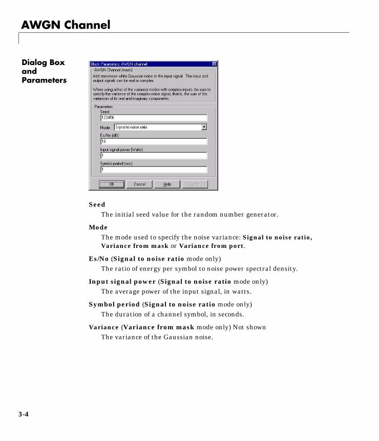
Dialog Box and Parameters
SeedThe initial seed value for the random number generator.
ModeThe mode used to specify the noise variance: Signal to noise ratio,Variance from mask or Variance from port.
Es/No (Signal to noise ratio mode only)The ratio of energy per symbol to noise power spectral density.
Input signal power (Signal to noise ratio mode only)The average power of the input signal, in watts.
Symbol period (Signal to noise ratio mode only)The duration of a channel symbol, in seconds.
Variance (Variance from mask mode only) Not shownThe variance of the Gaussian noise.
3-4

AWGN Channel
Characteristics Direct Feedthrough Yes
Sample Time Discrete, Inherited
Scalar Expansion N/A
Vectorized No
Complex Yes
3-5

Block Interleave
3Block InterleavePurpose Compute block interleaving or block deinterleaving.
Library Utility Functions
Description Block interleaving is accomplished in two steps.
• The input sequence is written row by row into an M-row by N-column(M-by-N) array.
• The output sequence is read column by column from this M-by-N array.
Deinterleaving switches the directions of the operations: the sequence iswritten into the array column by column and read out row by row.
Block interleaving is implemented using the Register Shift, Triggered BufferDown, and Triggered Signal Switch (vector re-arrangement) utility blocks.
Interleaving is often used with error-control coding. Typically, you select theinterleave parameters so that the number of columns, N, is greater than theexpected burst lengths. The choice of the number of rows depends on the typeof error-control coding scheme used. For block coding, the number of rowsshould be greater than the codeword length; thus, a burst of length N can causeat most a single error in any block codeword.
The timing for starting to fill the frame is very important. A block deinterleaveshould be synchronized with the block interleave in order to be able to recoverthe interleaved symbols. The delay is M*N symbols for each block (interleaverand deinterleaver).
Dialog Box and Parameters
3-6
Block Interleave
Input code row length (N)The number of columns in the array.
Interleave row number (M)The number of rows in the array.
Note: To use Block Interleave for deinterleaving, reverse the N and Mparameter settings.
Characteristics Direct Feedthrough Yes
Sample Time Triggered action. Inherits the sample time from theblocks that input to this block.
Scalar Expansion N/A
Vectorized N/A
Complex No
3-7

BPSK Demod
3BPSK DemodPurpose Demodulate BPSK modulated signal.
Library Version 1.3 Passband Digital Modulation/Demodulation
Description The BPSK (binary phase shift keying) Demodulation block demodulates theBPSK Mod signal. This block uses the Corr BPSK Demod block.
BPSK Demod is a passband simulation block. There are three time relatedvariables in this block: symbol interval (Td), carrier frequency (fc), andsimulation sample time (Ts). You must select values for these variables so thatthey satisfy the mathematical relations below.
This block receives a modulated analog signal as input. It outputs ademodulated binary signal.
Dialog Box and Parameters
Symbol interval, Carrier frequency, Initial phaseMatch these parameters to the ones used in the corresponding BPSK Modblock. The offset value in Symbol interval can be different.
Sample timeThe block’s sample time.
Td 1 fc⁄ 2Ts> >
3-8

BPSK Demod
Characteristics
Pair Block BPSK Mod
Direct Feedthrough Yes
Sample Time Discrete
Scalar Expansion N/A
Vectorized No
Complex No
3-9

BPSK Map
3BPSK MapPurpose Map a binary signal to phase shift for phase modulation.
Library Version 1.3 Passband Digital Modulation/Demodulation
Description The BPSK (binary phase shift keying) Map block maps the digital input signalto an analog signal for Phase Modulation (PM). If the input signal is 0, thephase shift is 0. If the input signal is 1, the phase shift is π. This block is aspecial case of the m-ary phase shift keying (MPSK) block in which M equals 2.
Dialog Box and Parameters
Input symbol interval and offsetThe sample time of the input symbol. When this parameter is atwo-element vector, the second element is the offset value.
Characteristics Direct Feedthrough Yes
Sample Time Discrete
Scalar Expansion N/A
Vectorized No
Complex No
3-10

BPSK Mod
3BPSK ModPurpose Modulate the input signal using binary phase shift keying method.
Library Version 1.3 Passband Digital Modulation/Demodulation
Description The BPSK (binary phase shift keying) Modulation block modulates the inputsignal. This block uses the BPSK Map block before feeding the signal to theDigital Phase Modulation (PM) block. Refer to their individual reference pagesfor descriptions of the techniques involved.
BPSK Mod is a passband simulation block. There are three time relatedvariables in this block: symbol interval (Td), carrier frequency (fc), andsimulation sample time (Ts). You must select values for these variables so thatthey satisfy the mathematical relations below.
The input signal to this block is a binary signal. The output is a modulatedanalog signal with a maximum amplitude equal to 1.
Dialog Box and Parameters
Symbol intervalThe sample time of the input symbol. When this parameter is atwo-element vector, the second element is the offset value.
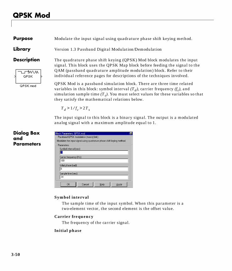
Carrier frequencyThe frequency of the carrier signal.
Td 1 fc⁄ 2Ts> >
3-11

BPSK Mod
Initial PhaseThe initial phase of the carrier signal.
Sample timeThe block’s sample time.
Characteristics
Pair Block BPSK Demod
Direct Feedthrough Yes
Sample Time Discrete
Scalar Expansion N/A
Vectorized No
Complex No
3-12

Convolutional Encoder
3Convolutional EncoderPurpose Convolutionally encode binary (0,1) input data.
Library Convolutional Codes, in Channel Coding
Description The Convolutional Encoder block encodes a sequence of binary input vectors toproduce a sequence of binary output vectors. The size of the input and outputvectors depends on the code rate. When you specify a rate k/n code, the input isa length k vector, and the output is a length n vector.
You can configure the Convolutional Encoder block to implement either afeedforward encoder or a feedback encoder. To specify a particular encoder, youmust also supply values for the parameters shown in the block mask below.
Dialog Box and Parameters
Constraint length1-by-k vector specifying the delay for each of the k input bit streams.
Code generatork-by-n matrix of octal numbers specifying the n output connections for eachof the k inputs.
Encoder typeFeedforward or Feedback.
3-13

Convolutional Encoder
Feedback connection (Feedback configuration only)1-by-k vector of octal numbers specifying the feedback connection for eachof the k inputs.
Reset inputWhen you check this box, the encoder has a second input port labeled Rst.A nonzero input value at this port causes the internal memory to be set toits initial state prior to processing the input data.
Note: Although the constraint length could be derived from the codegenerator and feedback connection parameters, you must enter thisparameter as a cross check for the code generator and feedback parameters.
Examples Example 1: Rate 2/3 Feedforward EncoderThe diagram below shows an example of a typical rate 2/3 feedforward encoder.
z-1 z-1 z-1 z-1
z-1 z-1 z-1
3-14
Convolutional Encoder
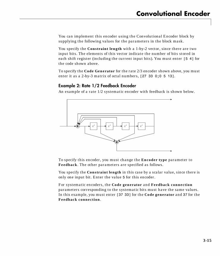
You can implement this encoder using the Convolutional Encoder block bysupplying the following values for the parameters in the block mask.
You specify the Constraint length with a 1-by-2 vector, since there are twoinput bits. The elements of this vector indicate the number of bits stored ineach shift register (including the current input bits). You must enter [5 4] forthe code shown above.
To specify the Code Generator for the rate 2/3 encoder shown above, you mustenter it as a 2-by-3 matrix of octal numbers, [27 33 0;0 5 13].
Example 2: Rate 1/2 Feedback EncoderAn example of a rate 1/2 systematic encoder with feedback is shown below.
To specify this encoder, you must change the Encoder type parameter toFeedback. The other parameters are specified as follows.
You specify the Constraint length in this case by a scalar value, since there isonly one input bit. Enter the value 5 for this encoder.
For systematic encoders, the Code generator and Feedback connectionparameters corresponding to the systematic bits must have the same values.In this example, you must enter [37 33] for the Code generator and 37 for theFeedback connection.
z-1 z-1 z-1 z-1
3-15

Convolutional Encoder
Characteristics
See Also Viterbi Decoder
Direct Feedthrough Yes
Sample Time Discrete, Inherited
Scalar Expansion N/A
Vectorized Yes
Complex No
3-16
Corr BPSK Demod
3Corr BPSK DemodPurpose Calculate binary phase shift keying demodulation correlation.
Library Version 1.3 Passband Digital Modulation/Demodulation
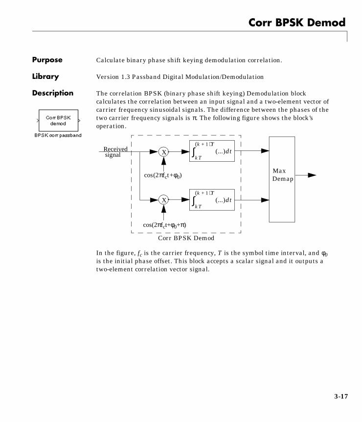
Description The correlation BPSK (binary phase shift keying) Demodulation blockcalculates the correlation between an input signal and a two-element vector ofcarrier frequency sinusoidal signals. The difference between the phases of thetwo carrier frequency signals is π. The following figure shows the block’soperation.
In the figure, fc is the carrier frequency, T is the symbol time interval, and φ0is the initial phase offset. This block accepts a scalar signal and it outputs atwo-element correlation vector signal.
X
X
cos(2πfct+φ0)
cos(2πfct+φ0+π)
MaxDemap
Corr BPSK Demod
Receivedsignal (...) td
kT
k 1+( )T
∫
(...) tdkT
k 1+( )T
∫
3-17
Corr BPSK Demod
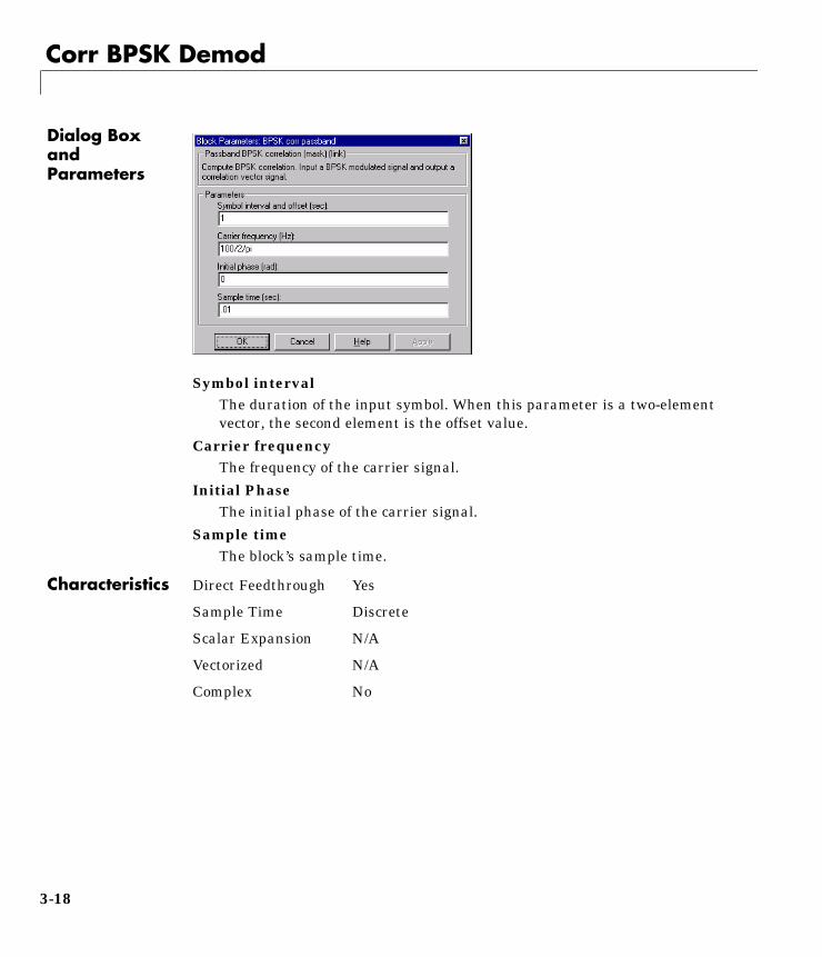
Dialog Box and Parameters
Symbol intervalThe duration of the input symbol. When this parameter is a two-elementvector, the second element is the offset value.
Carrier frequencyThe frequency of the carrier signal.
Initial PhaseThe initial phase of the carrier signal.
Sample timeThe block’s sample time.
Characteristics Direct Feedthrough Yes
Sample Time Discrete
Scalar Expansion N/A
Vectorized N/A
Complex No
3-18
Data Mapper
3Data MapperPurpose Map integer symbols from one coding scheme to another.
Library Utility Functions
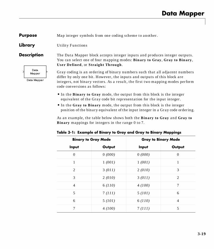
Description The Data Mapper block accepts integer inputs and produces integer outputs.You can select one of four mapping modes: Binary to Gray, Gray to Binary,User Defined, or Straight Through.
Gray coding is an ordering of binary numbers such that all adjacent numbersdiffer by only one bit. However, the inputs and outputs of this block areintegers, not binary vectors. As a result, the first two mapping modes performcode conversions as follows:
• In the Binary to Gray mode, the output from this block is the integerequivalent of the Gray code bit representation for the input integer.
• In the Gray to Binary mode, the output from this block is the integerposition of the binary equivalent of the input integer in a Gray code ordering.
As an example, the table below shows both the Binary to Gray and Gray toBinary mappings for integers in the range 0 to 7.
Table 3-1: Example of Binary to Gray and Gray to Binary Mappings
Binary to Gray Mode Gray to Binary Mode
Input Output Input Output
0 0 (000) 0 (000) 0
1 1 (001) 1 (001) 1
2 3 (011) 2 (010) 3
3 2 (010) 3 (011) 2
4 6 (110) 4 (100) 7
5 7 (111) 5 (101) 6
6 5 (101) 6 (110) 4
7 4 (100) 7 (111) 5
3-19
Data Mapper
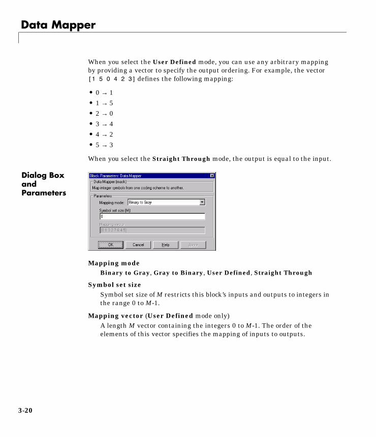
When you select the User Defined mode, you can use any arbitrary mappingby providing a vector to specify the output ordering. For example, the vector[1 5 0 4 2 3] defines the following mapping:
••••••
When you select the Straight Through mode, the output is equal to the input.
Dialog Box and Parameters
Mapping modeBinary to Gray, Gray to Binary, User Defined, Straight Through
Symbol set sizeSymbol set size of M restricts this block’s inputs and outputs to integers inthe range 0 to M-1.
Mapping vector (User Defined mode only)A length M vector containing the integers 0 to M-1. The order of theelements of this vector specifies the mapping of inputs to outputs.
0 1→1 5→2 0→3 4→4 2→5 3→
3-20

Data Mapper
Characteristics Direct Feedthrough Yes
Sample Time Discrete
Scalar Expansion N/A
Vectorized N/A
Complex No
3-21
Descrambler
3DescramblerPurpose Descramble the input signal.
Library Utility Functions
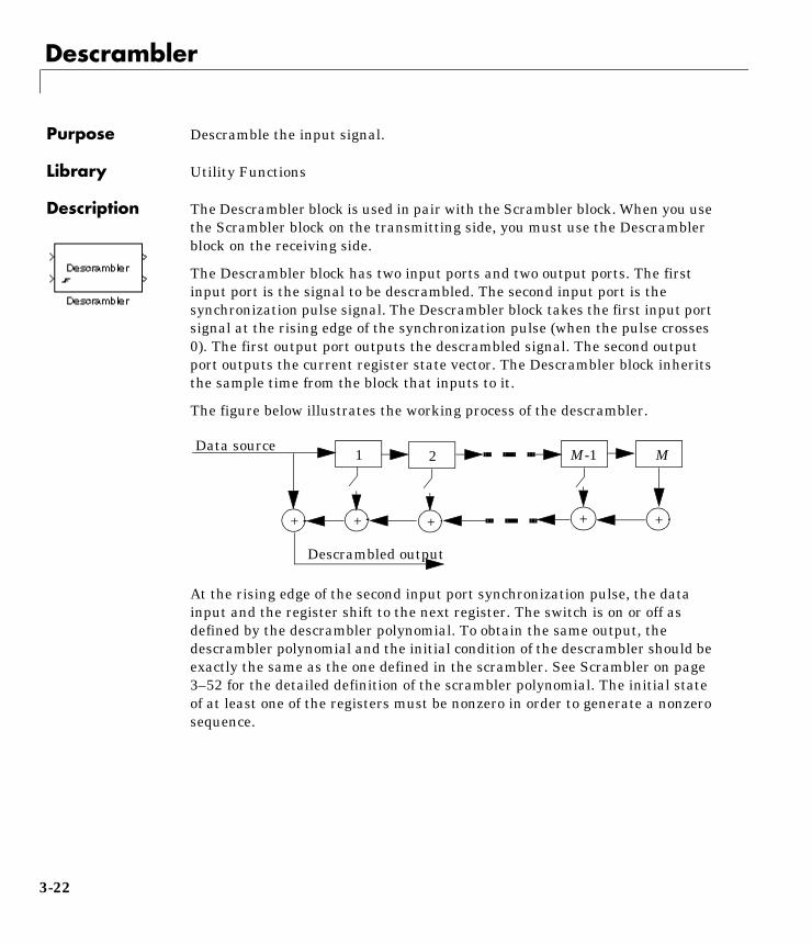
Description The Descrambler block is used in pair with the Scrambler block. When you usethe Scrambler block on the transmitting side, you must use the Descramblerblock on the receiving side.
The Descrambler block has two input ports and two output ports. The firstinput port is the signal to be descrambled. The second input port is thesynchronization pulse signal. The Descrambler block takes the first input portsignal at the rising edge of the synchronization pulse (when the pulse crosses0). The first output port outputs the descrambled signal. The second outputport outputs the current register state vector. The Descrambler block inheritsthe sample time from the block that inputs to it.
The figure below illustrates the working process of the descrambler.
At the rising edge of the second input port synchronization pulse, the datainput and the register shift to the next register. The switch is on or off asdefined by the descrambler polynomial. To obtain the same output, thedescrambler polynomial and the initial condition of the descrambler should beexactly the same as the one defined in the scrambler. See Scrambler on page3–52 for the detailed definition of the scrambler polynomial. The initial stateof at least one of the registers must be nonzero in order to generate a nonzerosequence.
+
1 2 M-1 M
++++
Data source
Descrambled output
3-22
Descrambler
Dialog Box and Parameters
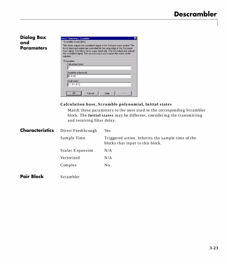
Calculation base, Scramble polynomial, Initial statesMatch these parameters to the ones used in the corresponding Scramblerblock. The Initial states may be different, considering the transmittingand receiving filter delay.
Characteristics
Pair Block Scrambler
Direct Feedthrough Yes
Sample Time Triggered action. Inherits the sample time of theblocks that input to this block.
Scalar Expansion N/A
Vectorized N/A
Complex No
3-23
Differential Decoder
3Differential DecoderPurpose Decode a binary signal using differential coding technique.
Library Utility Functions
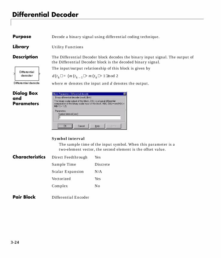
Description The Differential Decoder block decodes the binary input signal. The output ofthe Differential Decoder block is the decoded binary signal.
The input/output relationship of this block is given by
where m denotes the input and d denotes the output.
Dialog Box and Parameters
Symbol intervalThe sample time of the input symbol. When this parameter is atwo-element vector, the second element is the offset value.
Characteristics
Pair Block Differential Encoder
d tk( ) m tk 1–( ) m tk( ) 1+ +( )mod 2=
Direct Feedthrough Yes
Sample Time Discrete
Scalar Expansion N/A
Vectorized Yes
Complex No
3-24

Differential Encoder
3Differential EncoderPurpose Encode a binary signal using differential coding technique.
Library Utility Functions
Description The Differential Encoder block encodes the binary input signal. The output ofthis block is the encoded binary signal.
The input/output relationship of this block is given by
where m denotes the input and d denotes the output.
Dialog Box and Parameters
Symbol intervalThe sample time of the input symbol. When this parameter is atwo-element vector, the second element is the offset value.
Characteristics
Pair Block Differential Decoder
d tk( ) d tk 1–( ) m tk( ) 1+ +( )mod 2=
Direct Feedthrough Yes
Sample Time Discrete
Scalar Expansion N/A
Vectorized Yes
Complex No
3-25

DPSK Demod
3DPSK DemodPurpose Demodulate DPSK modulated signal.
Library Digital Passband Modulation, in Modulation
Description The DPSK (differential phase shift keying) Demodulation block demodulatesthe DPSK Mod signal. The block uses the digital MPSK Demod block and theDifferential Decoder block. Refer to their individual reference pages fordescriptions of the techniques involved.
DPSK Demod is a passband simulation block. There are three time relatedvariables in this block: symbol interval (Td), carrier frequency (fc), andsimulation sample time (Ts). You must select values for these variables so thatthey satisfy the mathematical relations below.
The input signal to this block is a modulated analog signal. The output is ademodulated binary signal.
Dialog Box and Parameters
Symbol interval, Carrier frequency, Initial phaseMatch these parameters to the ones used in the corresponding DPSK Modblock. The offset value in Symbol interval can be different.
Sample time (sec)The block’s sample time in seconds.
Td 1 fc⁄ 2Ts> >
3-26
DPSK Demod
Characteristics
Pair Block DPSK Mod
Direct Feedthrough Yes
Sample Time Discrete
Scalar Expansion N/A
Vectorized N/A
Complex No
3-27

DPSK Mod
3DPSK ModPurpose Modulate the input signal using differential phase shift keying method.
Library Digital Passband Modulation, in Modulation
Description The DPSK (differential phase shift keying) Modulation block modulates theinput signal. The block uses the Differential Encoder block before feeding thesignal to the digital MPSK Mod block. Refer to their individual reference pagesfor descriptions of the techniques involved.
DPSK Mod is a passband simulation block. There are three time relatedvariables in this block: symbol interval (Td), carrier frequency (fc), andsimulation sample time (Ts). You must select values for these variables so thatthey satisfy the mathematical relations below.
The input signal to the DPSK Mod block is a binary signal. The output is amodulated analog signal with a maximum amplitude equal to 1.
Dialog Box and Parameters
Symbol intervalThe duration of the input symbol. When this parameter is a two-elementvector, the second element is the offset value.
Carrier frequencyThe frequency of the carrier signal.
Td 1 fc⁄ 2Ts> >
3-28

DPSK Mod
Initial phaseThe initial phase of the carrier signal.
Sample timeThe block’s sample time.
Characteristics
Pair Block DPSK Demod
Direct Feedthrough Yes
Sample Time Discrete
Scalar Expansion N/A
Vectorized N/A
Complex No
3-29

Error Rate Calculation
3Error Rate CalculationPurpose Compute the bit error rate or symbol error rate of input data.
Library Comm Sinks
Description The Error Rate Calculation block takes input data from a transmitter andcompares it with input data from a receiver. It calculates the error rate as arunning statistic, by dividing the total number of data elements that are notequal by the total number of input data elements from one source.
This block adapts to either scalar or vector input. For vector inputs, the countof the number of elements compared at each sample time increases by thelength of the vector.
You can easily compute symbol or bit error rates because the Error RateCalculation block does not consider the magnitude of the difference betweeninput data elements. If the inputs are bits, this block computes the bit errorrate. If the inputs are symbols, the result is the symbol error rate.
The data produced at the output of the Error Rate Calculation block is a vectorwhose entries correspond to:
• The error rate
• The number of error events
• The total number of input events
You can configure this block to provide this output data to the workspace or toa port. When you write the data to the workspace, the values that are storedare the values that are current at the time you stop the simulation. To observethe running error statistics, you must provide the data to a port.
You can optionally configure this block with a reset port. When the reset portinput is nonzero, the Error Rate Calculation block clears the error statistics.
Combining these two options, you can configure the Error Rate Calculationblock in one of the following four modes:
• No reset, output to workspace (first block shown)
• External reset, output to workspace (second block shown)
• No reset, output to port (third block shown)
• External reset, output to port (fourth block shown)
3-30

Error Rate Calculation
Dialog Box and Parameters
Sample timeSample time of the transmit and receive input data.
Receive delayNumber of samples by which the received data lags behind the transmitteddata.
Output data toWorkspace or Port, depending on where you want to send the output data.
Workspace name (only if the Output data option Workspace is selected)Name of workspace variable for output data vector.
Reset portWhen you check this box, this block has a second input port labeled Rst.
Characteristics Direct Feedthrough No
Sample Time Discrete
Scalar Expansion N/A
Vectorized Yes
Complex No
3-31
MSK Demod
3MSK DemodPurpose Demodulate MSK modulated signal.
Library Digital Passband Modulation, in Modulation
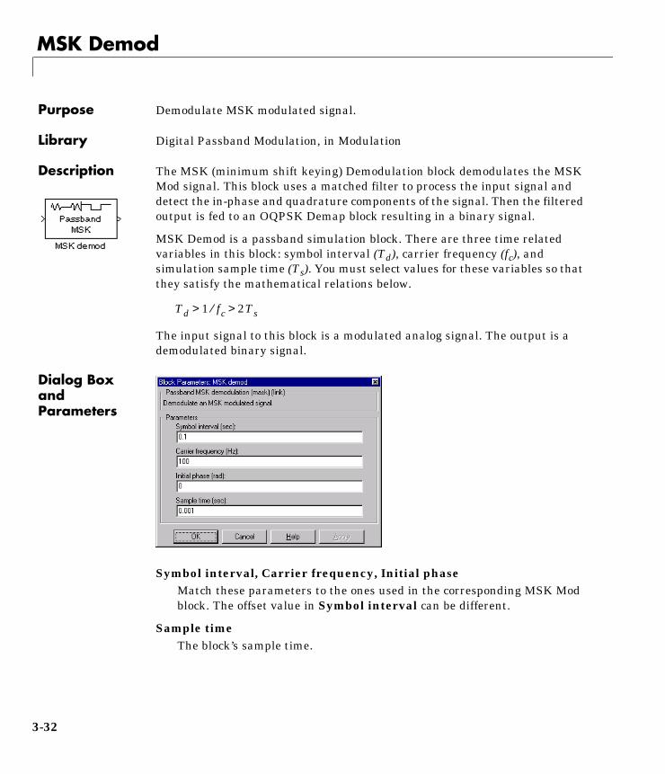
Description The MSK (minimum shift keying) Demodulation block demodulates the MSKMod signal. This block uses a matched filter to process the input signal anddetect the in-phase and quadrature components of the signal. Then the filteredoutput is fed to an OQPSK Demap block resulting in a binary signal.
MSK Demod is a passband simulation block. There are three time relatedvariables in this block: symbol interval (Td), carrier frequency (fc), andsimulation sample time (Ts). You must select values for these variables so thatthey satisfy the mathematical relations below.
The input signal to this block is a modulated analog signal. The output is ademodulated binary signal.
Dialog Box and Parameters
Symbol interval, Carrier frequency, Initial phaseMatch these parameters to the ones used in the corresponding MSK Modblock. The offset value in Symbol interval can be different.
Sample timeThe block’s sample time.
Td 1 fc⁄ 2Ts> >
3-32

MSK Demod
Characteristics
Pair Block MSK Mod
Direct Feedthrough Yes
Sample Time Discrete
Scalar Expansion N/A
Vectorized N/A
Complex No
3-33

MSK Mod
3MSK ModPurpose Modulate the input signal using minimum shift keying method.
Library Digital Passband Modulation, in Modulation
Description The MSK (minimum shift keying) Modulation block modulates the binaryinput signal. The block uses the OQPSK Map block to map the binary inputsignal to the in-phase component cI(t) and quadrature component cQ(t). Theoutput of the MSK Mod is s(t) where
MSK Mod is implemented based on the block diagram structure in thefollowing figure.
MSK Mod is a passband simulation block. There are three time relatedvariables in this block: symbol interval (Td), carrier frequency (fc), andsimulation sample time (Ts). You must select values for these variables so thatthey satisfy the mathematical relations below.
The input signal to this block is a binary signal. The output is a modulatedanalog signal with a maximum amplitude equal to 1.
s t( ) cI t( )πt2T-------
2πfctcoscos cQ t( )πt2T-------
sin 2sin πfct+=
+OQPSKmap
m(t)cI(t)
cQ(t)
+
+
+
-
X
X
s(t)
12--- 2πfct
πt2T-------+
cos
12--- 2πfct
πt2T-------–
cos
Td 1 fc⁄ 2Ts> >
3-34
MSK Mod
Dialog Box and Parameters
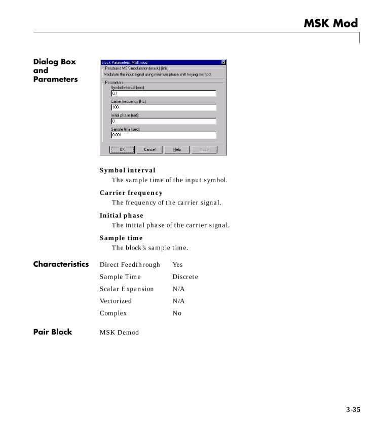
Symbol intervalThe sample time of the input symbol.
Carrier frequencyThe frequency of the carrier signal.
Initial phaseThe initial phase of the carrier signal.
Sample timeThe block’s sample time.
Characteristics
Pair Block MSK Demod
Direct Feedthrough Yes
Sample Time Discrete
Scalar Expansion N/A
Vectorized N/A
Complex No
3-35

OQPSK Demap
3OQPSK DemapPurpose Reverse OQPSK map converted signal.
Library Digital Passband Modulation, in Modulation
Description The OQPSK (offset quadrature phase shift keying) Demap block reverses anOQPSK Map converted signal. The inputs to this block are in-phase andquadrature components of the QADM (passband analog quadrature amplitudedemodulation) signal. The output of this block is a scalar binary signal, withsample time T. Refer to the OQPSK Map block description for the conversiontechnique.
Dialog Box and Parameters
Symbol interval and offsetThe sample time of the input symbol. When this parameter is atwo-element vector, the second element is the offset value.
Characteristics
Pair Block OQPSK Map
Direct Feedthrough Yes
Sample Time Discrete
Scalar Expansion N/A
Vectorized N/A
Complex No
3-36
OQPSK Demod
3OQPSK DemodPurpose Demodulate OQPSK modulated signal.
Library Digital Passband Modulation, in Modulation
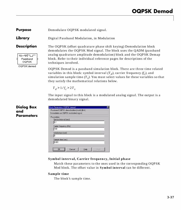
Description The OQPSK (offset quadrature phase shift keying) Demodulation blockdemodulates the OQPSK Mod signal. The block uses the QADM (passbandanalog quadrature amplitude demodulation) block and the OQPSK Demapblock. Refer to their individual reference pages for descriptions of thetechniques involved.
OQPSK Demod is a passband simulation block. There are three time relatedvariables in this block: symbol interval (Td), carrier frequency (fc), andsimulation sample time (Ts). You must select values for these variables so thatthey satisfy the mathematical relations below.
The input signal to this block is a modulated analog signal. The output is ademodulated binary signal.
Dialog Box and Parameters
Symbol interval, Carrier frequency, Initial phaseMatch these parameters to the ones used in the corresponding OQPSKMod block. The offset value in Symbol interval can be different.
Sample timeThe block’s sample time.
Td 1 fc⁄ 2Ts> >
3-37

OQPSK Demod
Characteristics
Pair Block OQPSK Mod
Direct Feedthrough Yes
Sample Time Discrete
Scalar Expansion N/A
Vectorized N/A
Complex No
3-38
OQPSK Map
3OQPSK MapPurpose Convert a binary scalar input signal to a binary vector output signal, whichincludes in-phase and quadrature components.
Library Digital Passband Modulation, in Modulation
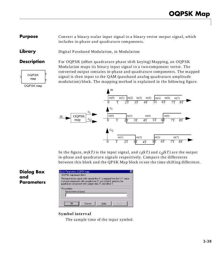
Description For OQPSK (offset quadrature phase shift keying) Mapping, an OQPSKModulation maps its binary input signal to a two-component vector. Theconverted output contains in-phase and quadrature components. The mappedsignal is then input to the QAM (passband analog quadrature amplitudemodulation) block. The mapping method is explained in the following figure.
In the figure, m(kT) is the input signal, and cI(kT) and cQ(kT) are the outputin-phase and quadrature signals respectively. Compare the differencesbetween this block and the QPSK Map block to see the time shifting difference.
Dialog Box and Parameters
Symbol intervalThe sample time of the input symbol.
0 T 2T 3T 4T 5T 6T 7T 8Tm(0) m(1) m(2) m(3) m(4) m(5) m(6) m(7)
0 T 2T 3T 4T 5T 6T 7T 8Tm(0) m(2) m(4) m(6)
m
cI
mcI
cQOQPSKmap
0 T 2T 3T 4T 5T 6T 7T 8Tm(1) m(3) m(5) m(7)
cQ
3-39
OQPSK Map
Characteristics
Pair Block OQPSK Demap
Direct Feedthrough Yes
Sample Time Discrete
Scalar Expansion N/A
Vectorized No
Complex No
3-40
OQPSK Mod
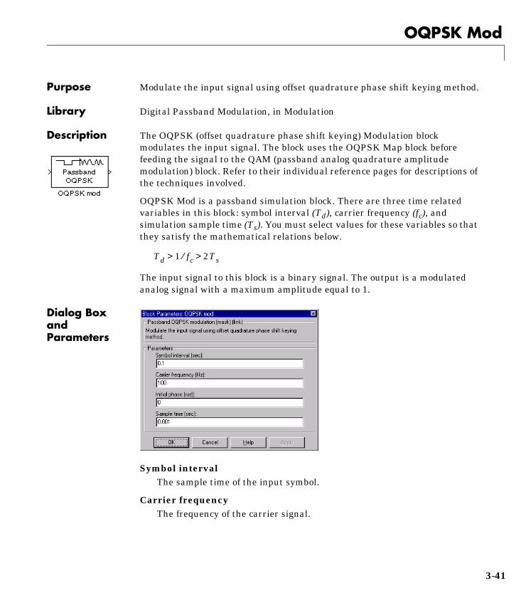
3OQPSK ModPurpose Modulate the input signal using offset quadrature phase shift keying method.
Library Digital Passband Modulation, in Modulation
Description The OQPSK (offset quadrature phase shift keying) Modulation blockmodulates the input signal. The block uses the OQPSK Map block beforefeeding the signal to the QAM (passband analog quadrature amplitudemodulation) block. Refer to their individual reference pages for descriptions ofthe techniques involved.
OQPSK Mod is a passband simulation block. There are three time relatedvariables in this block: symbol interval (Td), carrier frequency (fc), andsimulation sample time (Ts). You must select values for these variables so thatthey satisfy the mathematical relations below.
The input signal to this block is a binary signal. The output is a modulatedanalog signal with a maximum amplitude equal to 1.
Dialog Box and Parameters
Symbol intervalThe sample time of the input symbol.
Carrier frequencyThe frequency of the carrier signal.
Td 1 fc⁄ 2Ts> >
3-41

OQPSK Mod
Initial phaseThe initial phase of the carrier signal.
Sample timeThe block’s sample time.
Characteristics
Pair Block OQPSK Demod
Direct Feedthrough Yes
Sample Time Discrete
Scalar Expansion N/A
Vectorized No
Complex No
3-42
PN Sequence
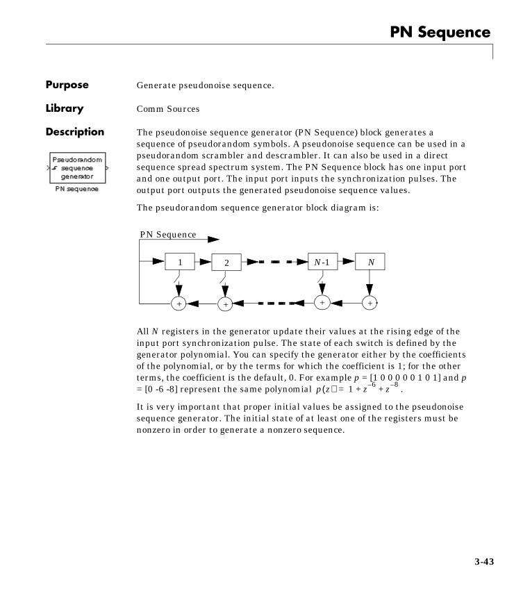
3PN SequencePurpose Generate pseudonoise sequence.
Library Comm Sources
Description The pseudonoise sequence generator (PN Sequence) block generates asequence of pseudorandom symbols. A pseudonoise sequence can be used in apseudorandom scrambler and descrambler. It can also be used in a directsequence spread spectrum system. The PN Sequence block has one input portand one output port. The input port inputs the synchronization pulses. Theoutput port outputs the generated pseudonoise sequence values.
The pseudorandom sequence generator block diagram is:
All N registers in the generator update their values at the rising edge of theinput port synchronization pulse. The state of each switch is defined by thegenerator polynomial. You can specify the generator either by the coefficientsof the polynomial, or by the terms for which the coefficient is 1; for the otherterms, the coefficient is the default, 0. For example p = [1 0 0 0 0 0 1 0 1] and p= [0 -6 -8] represent the same polynomial .
It is very important that proper initial values be assigned to the pseudonoisesequence generator. The initial state of at least one of the registers must benonzero in order to generate a nonzero sequence.
1 2 N-1 N
++++
PN Sequence
p z( ) 1 z 6– z 8–+ +=
3-43

PN Sequence
Dialog Box and Parameters
Calculation baseThe base used by the block for calculation.
Generator polynomialGenerator polynomial. Determines the shift register feedback connections.
Initial statesInitial states of the registers. The vector length of this entry must equal theorder of the generator polynomial. The elements of the vector are restrictedby the Calculation base.
Characteristics Direct Feedthrough Yes
Sample Time Triggered action. Inherits the sample time of theblocks that input to this block.
Scalar Expansion N/A
Vectorized No
Complex No
3-44
QPSK Demap
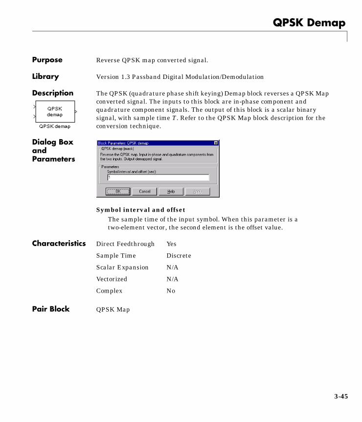
3QPSK DemapPurpose Reverse QPSK map converted signal.
Library Version 1.3 Passband Digital Modulation/Demodulation
Description The QPSK (quadrature phase shift keying) Demap block reverses a QPSK Mapconverted signal. The inputs to this block are in-phase component andquadrature component signals. The output of this block is a scalar binarysignal, with sample time T. Refer to the QPSK Map block description for theconversion technique.
Dialog Box and Parameters
Symbol interval and offsetThe sample time of the input symbol. When this parameter is atwo-element vector, the second element is the offset value.
Characteristics
Pair Block QPSK Map
Direct Feedthrough Yes
Sample Time Discrete
Scalar Expansion N/A
Vectorized N/A
Complex No
3-45
QPSK Demod
3QPSK DemodPurpose Demodulate QPSK modulated signal.
Library Version 1.3 Passband Digital Modulation/Demodulation
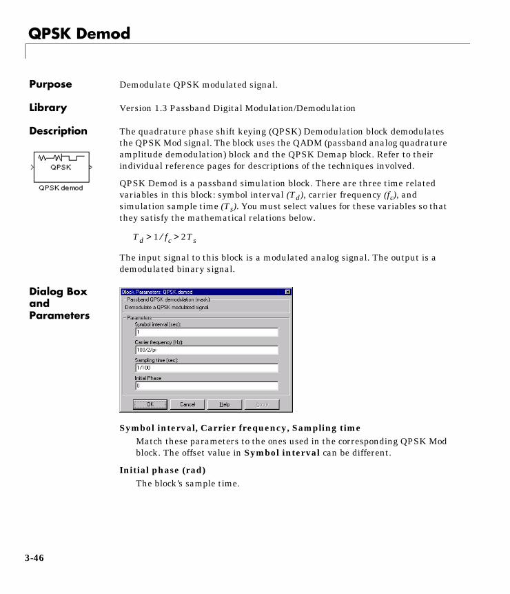
Description The quadrature phase shift keying (QPSK) Demodulation block demodulatesthe QPSK Mod signal. The block uses the QADM (passband analog quadratureamplitude demodulation) block and the QPSK Demap block. Refer to theirindividual reference pages for descriptions of the techniques involved.
QPSK Demod is a passband simulation block. There are three time relatedvariables in this block: symbol interval (Td), carrier frequency (fc), andsimulation sample time (Ts). You must select values for these variables so thatthey satisfy the mathematical relations below.
The input signal to this block is a modulated analog signal. The output is ademodulated binary signal.
Dialog Box and Parameters
Symbol interval, Carrier frequency, Sampling timeMatch these parameters to the ones used in the corresponding QPSK Modblock. The offset value in Symbol interval can be different.
Initial phase (rad)The block’s sample time.
Td 1 fc⁄ 2Ts> >
3-46
QPSK Demod
Characteristics
Pair Block QPSK Mod
Direct Feedthrough Yes
Sample Time Discrete
Scalar Expansion N/A
Vectorized N/A
Complex No
3-47

QPSK Map
3QPSK MapPurpose Convert a binary scalar input signal to a binary vector output signal, whichincludes in-phase and quadrature components.
Library Version 1.3 Passband Digital Modulation/Demodulation
Description For quadrature phase shift keying (QPSK) mapping, a QPSK modulation mapsits binary input signal to a two-component vector. The converted outputcontains in-phase and quadrature components. The mapped signal is theninput to the QAM (passband analog quadrature amplitude modulation) block.The mapping method is explained in the following figure.
In the figure, m(kT) is the input signal, and cI(kT) and cQ(kT) are the outputin-phase and quadrature signals respectively. As illustrated in this figure,c((k+1)T) outputs the input signal of c((k+1)T). This makes the systemnoncausal. To implement the block, the time interval delay, T, is introduced.
Dialog Box and Parameters
0 T 2T 3T 4T 5T 6T 7T 8Tm(0) m(1) m(2) m(3) m(4) m(5) m(6) m(7)
0 T 2T 3T 4T 5T 6T 7T 8Tm(0) m(2) m(4) m(6)
m
cI
0 T 2T 3T 4T 5T 6T 7T 8Tm(1) m(3) m(5) m(7)
cQ
mcI
cQQPSKmap
3-48

QPSK Map
Symbol intervalThe sample time of the input symbol. When this parameter is atwo-element vector, the second element is the offset value.
Characteristics
Pair Block QPSK Demap
Direct Feedthrough Yes
Sample Time Discrete
Scalar Expansion N/A
Vectorized N/A
Complex No
3-49
QPSK Mod
3QPSK ModPurpose Modulate the input signal using quadrature phase shift keying method.
Library Version 1.3 Passband Digital Modulation/Demodulation
Description The quadrature phase shift keying (QPSK) Mod block modulates the inputsignal. This block uses the QPSK Map block before feeding the signal to theQAM (passband quadrature amplitude modulation) block. Refer to theirindividual reference pages for descriptions of the techniques involved.
QPSK Mod is a passband simulation block. There are three time relatedvariables in this block: symbol interval (Td), carrier frequency (fc), andsimulation sample time (Ts). You must select values for these variables so thatthey satisfy the mathematical relations below.
The input signal to this block is a binary signal. The output is a modulatedanalog signal with a maximum amplitude equal to 1.
Dialog Box and Parameters
Symbol intervalThe sample time of the input symbol. When this parameter is atwo-element vector, the second element is the offset value.
Carrier frequencyThe frequency of the carrier signal.
Initial phase
Td 1 fc⁄ 2Ts> >
3-50

QPSK Mod
The initial phase of the carrier signal.
Sample timeThe block’s sample time.
Characteristics
Pair Block QPSK Demod
Direct Feedthrough Yes
Sample Time Discrete
Scalar Expansion N/A
Vectorized N/A
Complex No
3-51
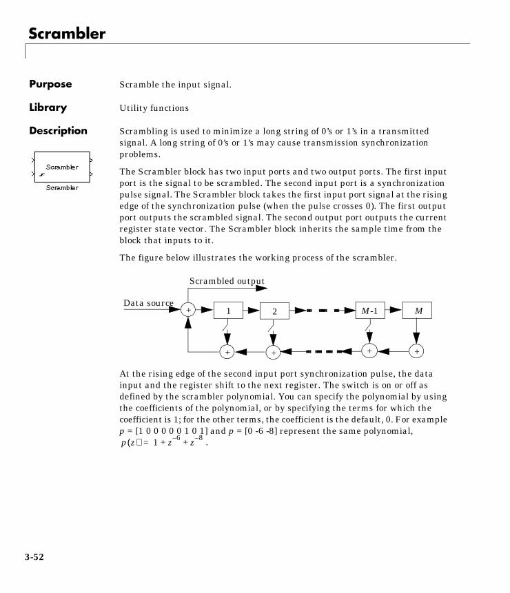
Scrambler
3ScramblerPurpose Scramble the input signal.
Library Utility functions
Description Scrambling is used to minimize a long string of 0’s or 1’s in a transmittedsignal. A long string of 0’s or 1’s may cause transmission synchronizationproblems.
The Scrambler block has two input ports and two output ports. The first inputport is the signal to be scrambled. The second input port is a synchronizationpulse signal. The Scrambler block takes the first input port signal at the risingedge of the synchronization pulse (when the pulse crosses 0). The first outputport outputs the scrambled signal. The second output port outputs the currentregister state vector. The Scrambler block inherits the sample time from theblock that inputs to it.
The figure below illustrates the working process of the scrambler.
At the rising edge of the second input port synchronization pulse, the datainput and the register shift to the next register. The switch is on or off asdefined by the scrambler polynomial. You can specify the polynomial by usingthe coefficients of the polynomial, or by specifying the terms for which thecoefficient is 1; for the other terms, the coefficient is the default, 0. For examplep = [1 0 0 0 0 0 1 0 1] and p = [0 -6 -8] represent the same polynomial,
.
+ 1 2 M-1 M
++++
Data source
Scrambled output
p z( ) 1 z 6– z 8–+ +=
3-52
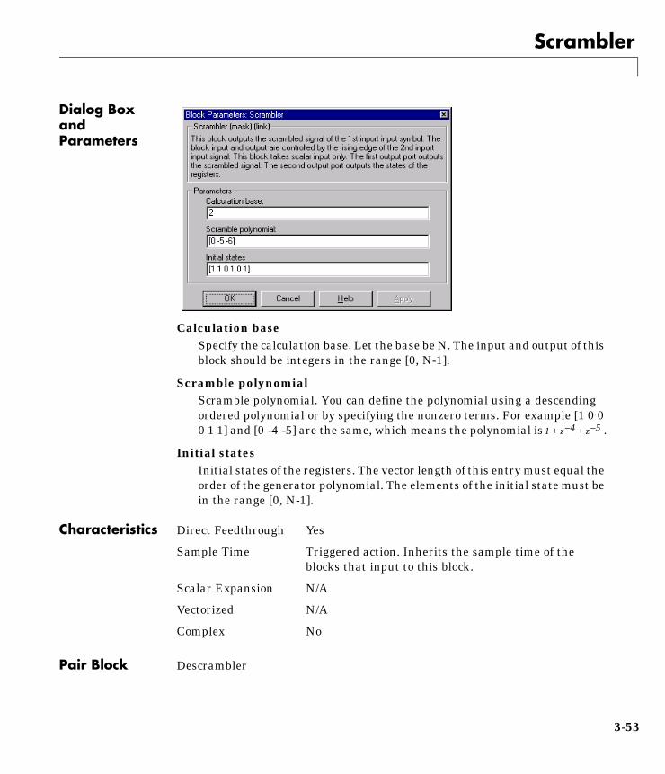
Scrambler
Dialog Box and Parameters
Calculation baseSpecify the calculation base. Let the base be N. The input and output of thisblock should be integers in the range [0, N-1].
Scramble polynomialScramble polynomial. You can define the polynomial using a descendingordered polynomial or by specifying the nonzero terms. For example [1 0 00 1 1] and [0 -4 -5] are the same, which means the polynomial is .
Initial statesInitial states of the registers. The vector length of this entry must equal theorder of the generator polynomial. The elements of the initial state must bein the range [0, N-1].
Characteristics
Pair Block Descrambler
1 z 4– z 5–+ +
Direct Feedthrough Yes
Sample Time Triggered action. Inherits the sample time of theblocks that input to this block.
Scalar Expansion N/A
Vectorized N/A
Complex No
3-53

Viterbi Decoder
3Viterbi DecoderPurpose Decode convolutionally encoded data using the Viterbi algorithm.
Library Convolutional Codes, in Channel Coding
Description The Viterbi Decoder block decodes a sequence of input symbols to produce asequence of binary output symbols.
This block has two sets of parameters:
• Parameters that specify the corresponding rate k/n convolutional encoder(constraint length, code generator, encoder type, and feedback connection)
• Parameters that specify the operation of the decoder (soft decision type,number of soft decision bits, traceback depth, and reset input)
For explanations of the parameters corresponding to the convolutionalencoder, see Convolutional Encoder on page 3–13.
Decision TypesWhen you set the decision type to unquantized, the decoder expects signed realinput values. It uses +1 to represent a logical zero and -1 to represent a logicalone.
When you set the decision type to hard decision, the decoder expects binaryinput values. It uses 0 to represent a logical zero and 1 to represent a logicalone.
When you set the decision type to soft decision, the decoder requires inputvalues in the range 0 to 2b-1, where b is the value of the number of soft decisionbits. For soft decisions, 0 represents the most confident decision for a logicalzero and 2b-1 represents the most confident decision for a logical one. Thevalues in between these extremes represent less confident decisions. As anexample, see the following table for information on how to interpret 3-bit softdecisions.
3-54
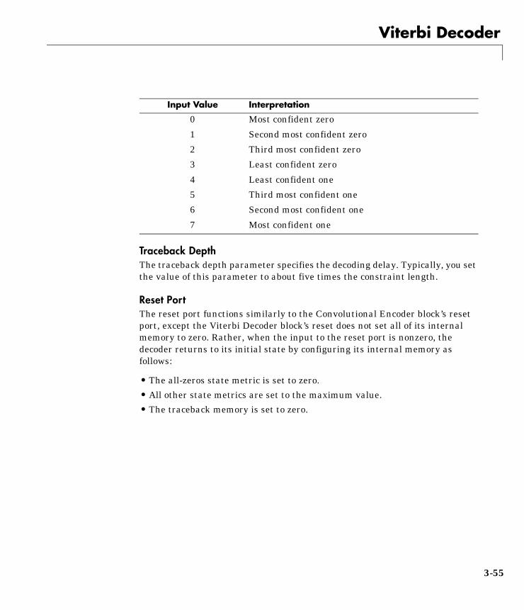
Viterbi Decoder
Traceback DepthThe traceback depth parameter specifies the decoding delay. Typically, you setthe value of this parameter to about five times the constraint length.
Reset PortThe reset port functions similarly to the Convolutional Encoder block’s resetport, except the Viterbi Decoder block’s reset does not set all of its internalmemory to zero. Rather, when the input to the reset port is nonzero, thedecoder returns to its initial state by configuring its internal memory asfollows:
• The all-zeros state metric is set to zero.
• All other state metrics are set to the maximum value.
• The traceback memory is set to zero.
Input Value Interpretation
0 Most confident zero
1 Second most confident zero
2 Third most confident zero
3 Least confident zero
4 Least confident one
5 Third most confident one
6 Second most confident one
7 Most confident one
3-55

Viterbi Decoder
Dialog Box and Parameters
Constraint length1-by-k vector specifying the delay for each of the k input bit streams.
Code generatork-by-n matrix of octal numbers specifying the n output connections for eachof the k inputs.
Encoder configurationFeedforward or Feedback.
Feedback connection (Feedback configuration only)1-by-k vector of octal numbers specifying the feedback connection for eachof the k inputs.
Decision typeUnquantized, Hard decision, or Soft decision.
Number of soft decision bits (Soft decision type only)The number of soft decision bits used to represent each input.
3-56
Viterbi Decoder
Traceback depthThe amount of delay before the decoder releases an output decoded bitdecision.
Reset portWhen you check this box, the decoder has a second input port labeled Rst.Providing a nonzero input value to this port causes the internal memory tobe set to its initial state prior to processing the input data.
Characteristics
See Also Convolutional Encoder
Direct Feedthrough Yes
Sample Time Discrete, Inherited
Scalar Expansion N/A
Vectorized Yes
Complex No
3-57

Viterbi Decoder
3-58
A
Corrections to User’s Guide
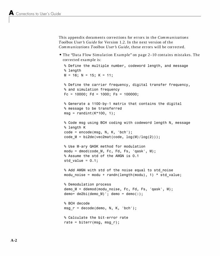
A Corrections to User’s Guide
A-2
This appendix documents corrections for errors in the CommunicationsToolbox User’s Guide for Version 1.2. In the next version of theCommunications Toolbox User’s Guide, these errors will be corrected.
• The “Data Flow Simulation Example” on page 2–10 contains mistakes. Thecorrected example is:% Define the multiple number, codeword length, and message % lengthM = 16; N = 15; K = 11;
% Define the carrier frequency, digital transfer frequency, % and simulation frequencyFc = 10000; Fd = 1000; Fs = 100000;
% Generate a 1100-by-1 matrix that contains the digital % message to be transferredmsg = randint(K*100, 1);
% Code msg using BCH coding with codeword length N, message % length Kcode = encode(msg, N, K, 'bch');code_M = bi2de(vec2mat(code, log(M)/log(2)));
% Use M-ary QASK method for modulationmodu = dmod(code_M, Fc, Fd, Fs, 'qask', M);% Assume the std of the AWGN is 0.1std_value = 0.1;
% Add AWGN with std of the noise equal to std_noisemodu_noise = modu + randn(length(modu), 1) * std_value;
% Demodulation processdemo_M = ddemod(modu_noise, Fc, Fd, Fs, 'qask', M);demo= de2bi(demo_M)'; demo = demo(:);
% BCH decodemsg_r = decode(demo, N, K, 'bch');
% Calculate the bit-error raterate = biterr(msg, msg_r);
• In the “Source Coding” tutorial on page 3-21, the following line appears inthe example:
[p_trans, partition, codebook] = dpcmopt(sig, 1, N)
The line should be:[p_trans, codebook, partition] = dpcmopt(sig, 1, N)
• In the “Example of a Linear Block Code” on page 3-32, the following lineappears in the example:
rcv = decode(code_noise,N,K ’block’, gen2par(G));
The line should be:
rcv= decode(code_noise,N,K,'linear', gen2par(G));
• In the example on page 6-74 (the reference page for the Reed-SolomonEncode Integer Vector In/Out block), the message vector [6 7 4 0 1] should be[6 7 4 0 4]. The codeword [3 2 6 7 4 0 1] should be [3 2 6 7 4 0 4].
• In the example on page 6-76 (the reference page for the Reed-SolomonDecode Integer Vector In/Out block), the codeword [3 2 6 7 4 0 1] should be[3 2 6 7 4 0 4]. The message vector [6 7 4 0 1] should be [6 7 4 0 4].
A-3

A Corrections to User’s Guide
A-4

Index
AAWGN Channel block 3-3
Bbinary phase shift keying 3-8, 3-11Block Interleave block 3-6BPSK Demod block 3-8BPSK Map block 3-10BPSK Mod block 3-11
Ccompatibility
Communications Toolbox Version 1.3 1-3MATLAB 1-2Simulink 1-2
Convolutional Encoder block 3-13convolutional encoding 2-16Corr BPSK Demod block 3-17
DData Mapper block 2-3, 3-19deinterleaving 3-6Descrambler block 3-22Differential Decoder block 3-24Differential Encoder block 3-25differential phase shift keying 3-26, 3-28DPSK Demod block 3-26DSPK Mod block 3-28
Eerasure insertion 2-19Error Rate Calculation block 2-11, 3-30
GGray coding 2-5, 2-9
Iinterleaving 3-6
Mminimum shift keying 3-32, 3-34MSK Demod block 3-32MSK Mod block 3-34
Ooffset quadrature phase shift keying 3-37, 3-41OQPSK Demap block 3-36OQPSK Demod block 3-37OQPSK Map block 3-39OQPSK Mod block 3-41
Pphase shift keying
binary 3-8, 3-11differential 3-26, 3-28minimum 3-32, 3-34offset quadrature 3-37, 3-41quadrature 3-46, 3-50
PN Sequence block 3-43pseudorandom sequence 3-43punctured coding 2-14, 2-17
QQPSK Demap block 3-45QPSK Demod block 3-46
I-1

Index
I-2
QPSK Map block 3-48QPSK Mod block 3-50quadrature phase shift keying 3-46, 3-50
SScrambler block 3-52
VViterbi Decoder block 3-54Viterbi decoding 2-20