foods and fads: the welfare impacts of rising quinoa...

Towson UniversityDepartment of Economics

Working Paper Series

Working Paper No. 2016-06

Foods and Fads: The Welfare Impacts ofRising Quinoa Prices in Peru

by Marc F. Bellemare, Johanna Fajardo-Gonzalez and Seth R. Gitter

March 2016

© 2016 by Author. All rights reserved. Short sections of text, not to exceed twoparagraphs, may be quoted without explicit permission provided that full credit, including© notice, is given to the source.

Foods and Fads: The Welfare Impacts of Rising Quinoa Prices in Peru*

March 16, 2016

Marc F. Bellemare† Johanna Fajardo-Gonzalez‡ Seth R. Gitter§

Abstract

Riding on a wave of interest in “superfoods” in rich countries, quinoa went in less than a decade from being largely unknown outside of South America to being an upper-class staple in the United States. As a consequence of that rapid rise in the popularity of quinoa, the price of quinoa tripled between 2006 and 2013. We study the impacts of rising quinoa prices on the welfare of Peruvian households. Using 10 years of a large-scale, nationally representative household survey, we combine pseudo-panel and difference-in-differences methods to look at the relationship between (i) the purchase price of quinoa and the value of household consumption, which we use here as a proxy for household welfare, and (ii) household quinoa production and household welfare. We find that increases in the purchase price of quinoa are associated with a significant increase in the welfare of the average household in areas where quinoa is consumed, which suggests that the quinoa price increase has had general equilibrium effects extending to non-producers. We also find that quinoa production is associated with a faster rate of growth of household welfare, but only at the height of the quinoa price boom. Our findings are robust to a number of different specifications.

Keywords: Quinoa, Commodity Price Shocks, Household Welfare, Peru

JEL Classification Codes: O12, Q12

* We thank Mercedez Callenes for help with the data. Bellemare is grateful to the University of Minnesota’s Institute for Advanced Studies for a fellowship during which this version of the article was written; Gitter is grateful to Towson University’s College of Business for funding part of the research in this article. We thank seminar audiences at GRADE, the Inter-American Development Bank, CIAT, IFPRI, and the University of Maryland, Baltimore County as well as conference participants at the 2015 Agricultural and Applied Economics Association annual meetings, the 2015 Midwest Economic Association conference, and the 2015 Midwest International Economic Development Conference for useful comments and suggestions. All remaining errors are ours. † Corresponding Author. Associate Professor, Department of Applied Economics and Director, Center for International Food and Agricultural Policy, University of Minnesota, Saint Paul, MN 55108, [email protected]. ‡ Ph.D. Candidate, Department of Applied Economics, University of Minnesota, Saint Paul, MN 55108, [email protected]. § Associate Professor, Department of Economics, Towson University, Towson, MD 21252, [email protected].

1

mailto:[email protected]



1. Introduction

Riding on a wave of interest in so-called superfoods1 in the United States and other rich countries,2

quinoa—a relatively high-protein grain that has been grown for millennia in the Andean regions of

Bolivia, Colombia, Ecuador, and Peru—went in less than a decade from being a largely unknown

commodity outside of South America to being an upper-class staple in those same rich countries. As

quinoa imports to the US increased more than tenfold, from about 5 million pounds per year in 2004 to

almost 65 million pounds per year in 2013 (DePillis, 2013), the price of quinoa tripled (Blythman, 2013).

Some have questioned the consequences of this increase in the popularity of quinoa, citing concerns

about the effects of rising quinoa prices on the welfare of individuals and households in places where

quinoa had traditionally been produced and consumed. A January 2013 article in the Guardian

(Manchester) made the following claim (Blythman, 2013):

[T]here is an unpalatable truth to face for those of us with a bag of quinoa in the larder. The appetite of countries such as ours for this grain has pushed up prices to such an extent that poorer people in Peru and Bolivia, for whom it was once a nourishing staple food, can no longer afford to eat it.

Three days later, an article in the Globe and Mail (Toronto) made the opposite claim (Saunders, 2013):

The people of the [Andean plateau] are indeed among the poorest in the Americas. But their economy is almost entirely agrarian. They are sellers—farmers or farm workers seeking the highest price and wage. The quinoa price rise is the greatest thing that has happened to them.

As one might expect from media accounts, neither claim was based in any serious empirical work. But

that net buyers of a commodity are made worse off and net sellers better off, at least in the short run,

by an increase in the price of that commodity is well-understood by economists (Deaton, 1989). That

1 The Oxford English Dictionary defines superfoods as foods “considered especially nutritious or otherwise beneficial to health and well-being” (OED, 2015). 2 With 50 percent of Peruvian quinoa going to the United States, the United States is the commodity’s largest export market (Andina, 2016). It is followed by Canada (8 percent), Australia (7 percent), Germany (6 percent), the United Kingdom (6 percent), the Netherlands (4 percent), France (3 percent) and Israel (3 percent).

2

being said, what are the longer-term,3 general equilibrium effects of that price increase for consumers?

And what is the effect of an international, positive price shock on the welfare of producers-cum-

consumers of that commodity?

We study the welfare impacts of rising quinoa prices on those households that have traditionally

produced and consumed it. To do so, we use 10 years of the Peruvian Encuesta Nacional de Hogares

(ENAHO), a large-scale, nationally representative household survey, to look at whether (i) there is a

systematic relationship between the value of household consumption, which we use here as a proxy for

household welfare (Deaton, 1997), and the local purchase price of quinoa for those households that

report consuming quinoa, and (ii) there is a systematic relationship between household welfare and the

price of quinoa for those households that report producing quinoa.

Our study period (i.e., 2004-2013) covers years both before and after the price of quinoa rose

sharply. Because the ENAHO is a repeated cross-section and is thus not longitudinal, we use pseudo-

panel techniques (Deaton, 1985; McKenzie, 2004; Christiaensen and Subbarao, 2005; Antman and

McKenzie, 2007a and 2007b; Cuesta et al., 2011), wherein we average over household-level measures

within each geographical unit and then treat those geographical units as our primary units of

observation.4 To study the relationship between the local purchase price of quinoa and household

consumption, we rely in turn on geographical unit fixed effects with a linear trend, with year fixed

effects, with geographical unit-specific trends, and with higher geographical unit-year fixed effects.5 To

study the relationship between quinoa production and household welfare, we combine pseudo-panel

3 By “longer-term,” we are referring to a time horizon that is longer (i.e., up to one year, given the frequency of our data) than Deaton’s (1989) short-term measure of welfare, and not to the long-term as it is typically understood in economics, i.e., the length of time required for all factors of production to be variable. 4 Peru is divided in 1,838 districts in 195 provinces in 25 departments. As a first check on the robustness of our results, we estimate each set of results three times, respectively treating districts, provinces, and departments as our units of observation. We discuss our estimation strategy in more details in section 3. 5 At the district level, this means province-year fixed effects. At the provincial level, this means department-year fixed effects.

3

techniques with a difference-in-differences design (Bertrand et al., 2004; Angrist and Pischke, 2009)

wherein the proportion of quinoa producers in a given geographical unit is the treatment variable.6

Our work is most closely related to the literature on the effects of commodity price shocks. This is a

sizeable literature, wherein scholars look at the effects of commodity price shocks on a host of

outcomes, from child outcomes (Cogneau and Jedwab, 2012) to conflict (Dube and Vargas, 2013) and

almost everything in between. Specifically, our work relates to the literature on the effects of

commodity price shocks—usually, food price shocks—on welfare. Ivanic and Martin (2008) study the

effects of higher global food prices on poverty in low-income countries. Using household surveys from

nine low-income countries, they find that the effects of higher food prices on poverty vary by country,

but also by commodity. Wodon and Zaman (2010) review the evidence looking specifically at sub-

Saharan Africa, and they find that higher food prices tend to increase the extent of poverty given that

net consumers tend to outnumber net producers of food. The study that is perhaps closest in spirit to

this one is an unpublished study by Zezza et al. (2008), who rely on household surveys in 11 countries to

look at how different groups of households are affected differently when food prices increase in an

effort to look at the distributional impacts of food price changes. One notable difference between our

work and the majority of studies in the commodity price shocks literature, however, is that while that

literature typically focuses on major food staples (e.g., maize, rice, wheat, etc.), we focus on a non-

staple. Additionally, the production of quinoa is concentrated in a specific region of the world, and little

quinoa is produced in the United States or Europe. This makes quinoa similar to other regionally

produced commodities, such as teff in Ethiopia and millet in Central Africa and India. The only other

6 Though it would a priori make sense to interact the proportion of quinoa producers in a given geographical unit with the international price of quinoa in an effort to exogenize the treatment variable (as in Dube and Vargas, 2013), the international price of quinoa here would be perfectly collinear with the year fixed effects we incorporate as part of our difference-in-differences estimates. We discuss this in more details in section 3, when we discuss our identification strategies.

4

economic study of the effect of rising quinoa prices has been by Stevens (2015), who finds that cultural

preference for quinoa in certain areas of Peru has not led to a worsening of nutritional outcomes.

Our results suggest that the increased international demand for quinoa and the resulting quinoa

price boom have had beneficial effects for consumers as well as for producers of quinoa in Peru. First,

we find a positive relationship between the price of quinoa and household welfare within the average

geographical unit-year wherein quinoa was consumed, which suggests that the sharp increase in the

price of quinoa has had positive general equilibrium effects on the welfare of the average household in

those geographical unit-year observations.7 Specifically, we find that for a 25-percent increase in the

price of quinoa—a change that is commensurate to the change in the purchase price of quinoa between

2012 and 2013, when international demand spiked—total household consumption increases on average

by about 1.75 percent.

Second, and in line with theoretical expectations (Deaton, 1989), we find a robust positive

relationship between household welfare and household quinoa production, but only in 2013. This

suggests that the welfare of quinoa producers grew significantly faster than that of other households,

but only at the height of the quinoa price boom.

Similarly, we find a robust negative relationship between the variability of household welfare within

a geographical unit and quinoa production, but only in 2012. This suggests that the variability of the

welfare of quinoa producers grew significantly less than that of other households once the price of

quinoa began rising sharply.

These pseudo-panel, difference-in-differences results are robust to whether (i) we exclude or

include the value of quinoa purchases from the value of a household’s total consumption, (ii) we

7 We focus on quinoa-consuming districts, households, and departments because those are the geographical units for which quinoa prices are available.

5

measure intensity of quinoa production in a region based on the proportion of quinoa-producing

households in 2004 (i.e., the first year of the period our study cover) in order to control for initial

conditions and partly obviate reverse causality concerns stemming from households deciding to grow

quinoa in response to increased quinoa prices) or in the year of observation, or (iii) we treat households

as our units of observation instead of geographical units. This positive relationship between household

welfare and quinoa production not only holds for the full sample of all geographical units, it also holds

for subsamples when we look at quinoa-producing areas only, at quinoa-consuming areas only, and at

areas whose consumption of quinoa is above the national average only.

The remainder of this article is organized as follows. In section 2, we present the data as well as

some descriptive statistics. Section 3 presents the empirical framework we develop to study the impacts

of rising quinoa prices on welfare, with particular emphasis on our identification strategy. In section 4,

we present and discuss our estimation results. Section 5 concludes with some policy recommendations

and directions for future research.

2. Data and Descriptive Statistics

We use data from the Peruvian Encuesta Nacional de Hogares (ENAHO), an annual household survey

conducted by the Peruvian government’s Instituto Nacional de Estadística e Informática (National

Institute of Statistics and Information). Because of its high quality and nationally representative

character, ENAHO data have been used frequently in economics. Among others, Dell (2010) has used the

ENAHO to study the long-term consequences of an extractive institution operating during colonial times

in Peru, Aragon and Rud (2013) have used the ENAHO to study the effects of a gold mine on local

incomes, and Galdo (2013) has used the ENAHO to study the long-run labor-market impacts of civil war.

The ENAHO sample is selected every year so as to be nationally representative. The data include

household-level sampling weights, which we use throughout. We use repeated cross sections from 2004

6

to 2013 inclusively, which encompass 227,400 household-year observations. We discuss in section 3

how the repeated cross-sectional nature of the data allows constructing a pseudo-panel.

Our outcome of interest is the total value of household consumption,8, 9 which we use here as a

proxy for household welfare. In developing countries such as Peru, where many households produce

food for their own subsistence, it is important to include the value of all consumption, and not just

purchases, in order to paint a more accurate portrait of welfare. For all households,10 purchased goods

represented roughly 75 percent of the value of total consumption (which includes household food

production). For quinoa-producing households, that number was closer to 60 percent. In other words,

40 percent of the total household consumption of quinoa-producing households is from non-purchased

goods, including household food production. Quinoa-producing households thus appear less integrated

in markets than non-producing households.

A comparison of mean household consumption among households that produce quinoa and those

that consumed quinoa but did not produce it is shown in Table 1. The most notable difference in Table 1

is that quinoa-producing households (third column of Table 1) consumed roughly 40 percent of what

8 We remove the value of quinoa that is produced and consumed by the household from our measure of household welfare so as to avoid biasing the relationship between quinoa prices and consumption by way of reverse causality. We explain our identification strategy further in section 3. 9 Annual total consumption is computed by INEI as the sum of (i) purchases of food, clothing, housing, fuel, electricity, furniture, housewares, health, transportation, communications, and entertainment. Individuals reported information in past month or past three months depending on expenditure group; (ii) expenditures on appliances, transport and others, (iii) expenditures on food consumed outside the household; (iv) expenditures on food to be consumed inside and outside the household, and (v) the reported value of own consumption, gifts, social programs, and payments in kind in the same expenditure groups. 10 We break our sample up into three non-mutually exclusive categories. “Quinoa producers” refers to households that report producing quinoa over the previous year, whether those households consumes quinoa or not; “quinoa consumers” and “quinoa non-consumers and non-producers” refer respectively to (i) households that report consuming quinoa over the last two weeks but not producing it over the last year, and (ii) households that neither produced quinoa over the last year nor consumed it over the previous two weeks if the household does not produce quinoa. Although it is common in the agricultural economics literature to split households between net buyers and net sellers of a commodity (see, for example, Bellemare et al., 2013), the different recall periods for production (i.e., past year) and consumption data (i.e., past two weeks) make this impossible in this article. However, fewer than 2 percent of producers reported purchasing quinoa in the last two weeks

7

quinoa-consuming households did at the beginning of the sample period.11 Households that consumed

but did not produce quinoa (fourth column of Table 1), however, had total household consumption

about 30 percent higher than that of households that neither consumed quinoa nor produce it. In other

words, consumers of quinoa look like they were substantially better off than the rest of the population.

This parallels how, at the international level, the demand from quinoa overwhelmingly comes from rich

countries.

Figure 1 shows time series of the consumption levels of quinoa producers, quinoa consumers, and

those that neither produced nor consumed quinoa wherein, for ease of comparison, baseline

consumption is set equal to 1 for each groups.12 Up until 2009, the welfare of quinoa consumers

increased at a faster rate than that of quinoa producers. Starting in 2010, however, quinoa producers

saw their welfare increase faster than quinoa consumers. In fact, and as the econometric analysis below

will confirm, at the peak of the quinoa price boom in 2013, the welfare of quinoa producers increased

much faster than that of quinoa consumers. Comparing quinoa-producing households one the one hand

with quinoa-consuming and quinoa neither consuming nor producing households on the other hand, the

welfare of quinoa producers increased by almost 50 percent over the period 2004-2013, whereas it

increased by about 30 percent for the other two groups of households.

In Table 2, we take a closer look at quinoa consumers. Over the sample period, one fourth to one

third of the households in our sample reported consuming quinoa in the two weeks before they were

surveyed, as shown in the second column of Table 2. Over these same two weeks, the average

household in the data purchased less than one kilogram of quinoa. Back-of-the-envelope calculations

based on Table 2 suggest that the total effect of price rises on consumer was small: At the beginning of

11 All monetary values are expressed in real terms in 2004 PEN. The 2004 PPP adjusted exchange rate was 1.3 Soles = $1 USD 12 Yearly departmental-level deflators are used to control for price changes

8

the sample period, households purchased roughly 22.6 kg per year (or 0.87 kg every two weeks), but the

real cost of this amount of quinoa rose roughly 100 PEN over the sample period, which is small in

comparison to overall consumption (about 20,000 PEN) for those households that do not produce

quinoa in 2013.

Over the sample period, quinoa purchases have fallen in response to the rising price of quinoa.

Indeed, the third and fifth columns of Table 2 show that the amount of quinoa purchased over the two

weeks before the survey fell by about 20 percent. Using the two-week purchase data, we estimated

annual purchases by multiplying by 26 to create a budget share. The budget share of quinoa rose as the

real price of quinoa paid by buyer more than doubled from 2004 to 2013. As noted above, quinoa

represents a very small share (i.e., less than 1 percent) of the budget of the average household in the

data, and the change in budget share between 2004 and 2013 is roughly 0.5 percent. Compared to the

budget share of staples in other developing countries, which often average over 50 percent (see, for

example, Barrett and Dorosh, 1996), quinoa does not seem to be a staple for households in Peru.

Indeed, even for the 99th percentile of quinoa buyers in the sample, the budget share of quinoa budget

share is only 10 percent.13

Table 3 shows some descriptive statistics for quinoa producers and sellers. Over the period 2004-

2013, roughly 3.6 percent of all households in the data grew any quinoa. Counter to what one might

expect given the quinoa price boom of 2012-2013, the percentage of producers in the data fell rather

than increased over the study period, dropping from 3.1 percent in 2011 to 2.81 percent in 2012, and

then to 2.63 percent in 2013.

13 Of those who purchased quinoa, those at the 99th percentile purchased 6kg over the last two weeks, or about 156kg per year. At a price of 7.83 PEN in 2013, this represents about 1,200 PEN, versus a total household consumption of about 12,000 PEN for this group, which amounts to a budget share of about 10 percent.

9

The second column of Table 3 shows that in any given year, less than 0.5 percent of the households

in our sample sold any quinoa. More interestingly for our purposes, the percentage of households that

sold some of their quinoa production (column 2 of Table 3) almost doubled between 2010 and 2011.

When looking only at the sub-sample of quinoa producers, the average household produced less than 90

kg of quinoa in the last 12 months, and over time, the volume of quinoa production has been U-shaped,

with the highest output levels per household at the beginning and at the end of our sample.

In our sample, over 98 percent of households that produced quinoa used at least some of it for their

own consumption. As shown in the fifth column of Table 3, however, the percentage of production used

for a household’s own consumption fell dramatically over the study period, from around three quarters

in 2004 to about one third in 2013.

We mentioned earlier that the international price of quinoa had tripled over the period 2004-2013.

Even more impressively, quinoa sellers have seen the real price of quinoa experience a more than

fourfold increase during that period. The rate at which the purchases price of quinoa rose (column 4 of

table 2) was less than the growth in the sales price (column 6 of table 3), and the farm gate-to-consumer

price ratio has increased from 43 percent to 60 percent between 2004 and 2013. This suggests that

quinoa producers have captured some of the gains from rising quinoa prices, though this is obviously far

from a formal test of that hypothesis, which is beyond the scope of this paper.

Lastly, the revenue of quinoa sellers grew almost sevenfold over the period 2004-2013 (seventh

column of table 3), although that increase has not been steady. There are also two jumps in revenue:

the first occurring between 2008 and 2009, when revenue almost doubled, and the second one

occurring between 2011 and 2012, when revenue increased by over 80 percent. This rise in revenue was

even more pronounced when looking at all quinoa farmers (eighth column of table 3), and not just to

quinoa sellers.

10

3. Empirical Framework

The ENAHO is a repeated cross-sectional household survey, so the usual panel methods favored by

applied microeconomists (i.e., household fixed effects) are not available in this context. A standard

strategy proposed by Deaton (1985) to overcome the type of data limitations one faces with repeated

cross-sections, is to rely on pseudo-panel methods. Intuitively, pseudo-panel methods treat groups of

observations (rather than the observations themselves) as units of analysis. In our application, instead of

treating the household as our unit of analysis, we treat geographical units as our units of analysis, and

we use geographical unit-level averages as our primary data. Recall from footnote 4 that Peru is divided

in 1,838 districts in 195 provinces in 25 departments. As a first check on the robustness of our results,

we estimate each set of results three times, respectively treating districts, provinces, and departments

as our units of observation.

The ENAHO has data on all 25 departments, on all but one of the 195 provinces, and on 1,401 of

1,838 districts. Given the random selection of communities and the nationally representative nature of

the ENAHO, those missing districts should not reduce the external validity of our results.

Pseudo-panel methods like the ones we use in this article have been effectively deployed to

estimate economic mobility (McKenzie, 2004; Cuesta et al. 2013) and to study poverty in developing

countries (Antman and McKenzie 2007a, 2007b; Christiaensen and Subbarao, 2005; Cruces et al., 2014).

Again, recall that in a pseudo-panel, the outcome variable (here, household welfare) and the treatment

variable (here, the price paid on average by a household for its quinoa when studying the welfare of

consumers, and whether a household grows quinoa when studying the welfare of producers) are

averaged across geographical unit. Because households are chosen at random within each geographic

region, the average among sampled households should track the average among population

households.

11

Our variable of interest is the total value of household consumption, which we use here as a proxy

for household welfare. For each geographical unit g, we compute the regional sample mean of the total

value of household consumption 𝑐𝑐�̅�𝑔𝑔𝑔 as the average of the total value of household consumption 𝑐𝑐𝑔𝑔ℎ𝑔𝑔

over all observed households h in the set 𝐻𝐻𝑔𝑔𝑔𝑔 of all households sampled in geographical unit g in year t,

such that

𝑐𝑐�̅�𝑔𝑔𝑔 = 1𝐻𝐻𝑔𝑔𝑔𝑔

∑ 𝑐𝑐ℎ𝑔𝑔𝑔𝑔𝐻𝐻𝑔𝑔𝑔𝑔𝑖𝑖=1 (1)

Here, pseudo-panel methods have two clear benefits. First, because the ENAHO covers over 20,000

households annually, the data is rich at both the national and sub-national levels, and statistical power is

not a concern. Second, as the number of households averaged over increases when computing the

geographical unit-level mean, the effect of potential error in the measurement of a particular

household’s consumption is reduced given that that error becomes spread out over more households. If

they were available to us, individual household fixed effects would allow correcting for time-invariant

measurement error; however, time-variant measurement error would still be present, and fixed effects

are thought to compound measurement error problems (Wooldridge, 2002).14 This would be an issue

especially regarding food consumption, where annual data is extrapolated from two weeks’ worth of

food consumption.15 Our use of pseudo-panel methods reduces this problem. Finally, we conduct a

robustness check on pseudo-panel results by estimating everything at the household level and

incorporating geographical unit fixed effects and year fixed effects. The household results, which

14 More specifically, Woolridge (2002, p.311) writes: “It is widely believed in econometrics that … FE transformations exacerbate measurement error bias (even though they eliminate heterogeneity bias). However, it is important to know that this conclusion rests on the classical errors-in-variables model under strict exogeneity, as well as on other assumptions.” 15 Because ENAHO households are interviewed year round, we conducted robustness checks using the household data in which we controlled for the survey date, to ensure that our results are not driven by seasonality. It turns out that our results are not driven by seasonality as can be seen in tables 6a-6c which present models with and without seasonality controls.

12

admittedly fail to control for time-invariant household characteristics, are consistent with the pseudo-

panel estimations.

As with many of the decisions one has to make when doing applied work, moving from the largest

(i.e., department) to the smallest (i.e., district) geographical unit involves a tradeoff. As the geographical

unit gets smaller, fewer observations go into making the geographical level-unit average, which

maximizes measurement error but also presents the most amount of statistical power in this context.

Conversely, as the geographical unit gets larger, there are fewer units of observations available for

analysis, which decreases statistical power, but which also minimizes measurement error problems. In

order to examine this tradeoff and to ensure that our results do not depend on the choice of

geographical unit, we estimate all of our specifications for each of the three levels of geographic

analysis.

We use two variables as our treatment variable, depending on whether we want to study the

welfare effects of rising quinoa prices on consumers or on producers of quinoa. For consumers, the

treatment variable is the average of the purchase price of quinoa within a geographical unit; because

purchase prices are observed only in those geographical units where people consume quinoa, this limits

our analysis of the welfare effects of rising quinoa prices on consumers to those geographical units

where quinoa was actually consumed. For producers, the treatment variable is the proportion of quinoa

producers within a geographical unit. Both treatment variables vary over time and across space, and it is

this spatio-temporal variation which we exploit here to identify the effects on welfare of rising quinoa

prices.

For our analysis of quinoa consumers, we regress the logarithm of the total value of household

consumption on the logarithm of the purchase price of quinoa, which yields the quinoa price elasticity of

household welfare.

13

For our analysis of quinoa producers, we regress the logarithm of the total value of household

consumption on the proportion of quinoa producers within a geographical unit. The proportion of

quinoa producers within a geographical unit allows the extent of quinoa production to vary over time as

households choose which crops to grow each year. Because households might decide to begin growing

quinoa because they expect to be better off from doing so, this exposes our estimates to an obvious

reverse causality issue. So as a robustness check intended to avoid that reverse causality problem, we

estimate specifications that control for baseline quinoa production in 2004 within each geographical

unit, using that 2004 measure across all years as our treatment variable, much like one would define

whether an observation has been treated in a difference-in-differences context. This serves as a time-

invariant measure of initial (production) conditions, and the results thereof constitute a first robustness

check on our producer results. The results using the time-invariant measure of production are consistent

with the time variant measure.

3.1. Estimation Strategy

3.1.1. Consumers

In the case of quinoa consumers, our equation of interest is such that

ln 𝑐𝑐𝑔𝑔𝑔𝑔 = 𝛼𝛼0 + 𝛼𝛼1 ln𝑝𝑝𝑔𝑔𝑔𝑔 + 𝛿𝛿𝑔𝑔 + 𝜏𝜏𝜏𝜏 + 𝜖𝜖𝑔𝑔𝑔𝑔, (2)

where, in a slight abuse of notation, ln 𝑐𝑐𝑔𝑔𝑔𝑔 is the mean of ln 𝑐𝑐ℎ𝑔𝑔𝑔𝑔 in geographical unit g in year t, ln𝑝𝑝𝑔𝑔𝑔𝑔 is

the mean of the purchase price of quinoa in geographical unit g in year t, 𝛿𝛿𝑔𝑔 is a vector of geographical-

unit fixed effects, t is a linear time trend, and 𝜖𝜖𝑔𝑔𝑔𝑔 is an error term with mean zero. In order to ensure

that our results are robust, we also estimate specifications where we replace the linear time trend with

(i) year fixed effects, (ii) own geographical unit-specific linear trends, (iii) higher-level geographical unit-

specific linear trends, when feasible, and (iv) higher-level geographical unit-year fixed effects, whenever

feasible.

14

Because equation (2) is estimated only for those geographical units where quinoa is consumed, 𝛼𝛼1 is

an estimate of the quinoa price elasticity of household welfare for those geographical units.

3.1.2. Producers

In the case of quinoa producers, our equation of interest is such that

ln 𝑐𝑐𝑔𝑔𝑔𝑔 = 𝜃𝜃0 + 𝛽𝛽0𝐷𝐷𝑔𝑔𝑔𝑔 + ∑ 𝜃𝜃𝑔𝑔𝑇𝑇𝑔𝑔 +2013𝑔𝑔=2005 ∑ 𝛽𝛽𝑔𝑔𝐷𝐷𝑔𝑔𝑔𝑔 × 𝑇𝑇𝑔𝑔 + 𝛾𝛾𝑔𝑔 + 𝜐𝜐𝑔𝑔𝑔𝑔2013

𝑔𝑔=2005 , (3)

where ln 𝑐𝑐𝑔𝑔𝑔𝑔 is the mean of ln 𝑐𝑐ℎ𝑔𝑔𝑔𝑔 in geographical unit g, 𝐷𝐷𝑔𝑔𝑔𝑔 is the proportion of households that

produce quinoa in geographical unit g, 𝑇𝑇𝑔𝑔 is a dummy variable equal to 1 in year t and equal to zero

otherwise, 𝛾𝛾𝑔𝑔 is a vector of geographical unit fixed effects, and 𝜐𝜐𝑔𝑔𝑔𝑔 is an error term with mean zero.

Recall that our data set covers the period 2004-2013, so the dummy for the year 2004 is omitted in

order to allow identifying the intercept. In order to obtain difference-in-differences estimates, 𝐷𝐷𝑔𝑔𝑔𝑔 and

𝑇𝑇𝑔𝑔 are interacted so as to estimate the difference in household welfare trends over time between

quinoa producers and quinoa non-producers. We cluster the standard errors at the level of the

geographical unit (i.e., district, province, or department) we use as our unit of analysis.

We perform four robustness checks in addition to the specification shown in equation (3). As a first

robustness check on our results for quinoa producers, we limit the sample only to quinoa-producing

regions, quinoa consuming areas and areas with above average consumption (Table 5). As a second

robustness check we use individual measure of quinoa production and change the unit of analysis to

household (Table 6). In Appendix (A.1) we include quinoa purchases in total household consumption.

Finally, in (A.2) we create a time invariant measure for quinoa producers, we replace 𝐷𝐷𝑔𝑔𝑔𝑔 with baseline

(i.e., 2004) quinoa production, 𝐷𝐷𝑔𝑔04. This means that we drop 𝛽𝛽0𝐷𝐷𝑔𝑔𝑔𝑔 and replace the time variant quinoa

measure with a time invariant measure for the interaction of quinoa with year fixed effects (i.e.,

∑ 𝛽𝛽𝑔𝑔𝐷𝐷042013𝑔𝑔=2005 ).

15

In addition to looking at whether quinoa production is associated with increases in household

consumption, we also look at whether quinoa production is associated with decreases in the variance of

household consumption within each geographical unit. Taking consumption expenditures as a proxy for

income (Deaton, 1997), any reduction in the variance of household consumption would mean that

quinoa production is associated with reductions in the risk and uncertainty faced by the households in

our sample, which suggests that those households might be producing quinoa as a means of coping with

risk. In other words, this would suggest that the production of quinoa has second-order effects on

welfare.

3.2. Identification Strategy

3.2.1. Consumers

The error term in equation (2) contains everything that goes unobserved in the same equation. Because

the households surveyed in the ENAHO are randomly selected, when controlling for the passage of time,

the households in a given geographical unit in a given year are similar to the households in the same

geographical unit the following year, and this both in terms of their observable and unobservable

characteristics. Thus, provided we account for the passage of time in our estimations, our use of

geographical unit-level fixed effects should take care of the time-invariant heterogeneity between

households.

To account for time-variant unobserved heterogeneity, we estimate several different specifications,

the idea being that if we find similar effects throughout, our results are more likely to be identified. First,

for our district-level analysis, on top of including district fixed effects, we estimate specifications with (i)

a linear time trend, (ii) year fixed effects, (iii) district-specific trends, (iv) province-specific trends, (v)

province-year fixed effects, (vi) department-specific trends, and (vii) department-year fixed effects.

Second, for our provincial-level analysis, on top of including province fixed effects, we estimate

specifications with (i) a linear time trend, (ii) year fixed effects, (iii) province-specific trends, (iv)

16

department-specific trends, and (v) department-year fixed effects. Finally, for our departmental-level

analysis, on top of including departmental fixed effects, we estimate specifications with (i) a linear time

trend, (ii) year fixed effects, and (iii) department-specific trends.

How do those specifications help identify the welfare effects of rising quinoa prices for consumers?

To help think through this, it helps to consider the three sources of statistical endogeneity, viz. (i)

reverse causality, (ii) unobserved heterogeneity, and (iii) measurement error. As regards reverse

causality, quinoa appears to be a normal or a luxury good, and as consumers get better off, they are

likely to start consuming more quinoa, which might cause quinoa prices to increase. Over the period

2004-2013, however, quinoa price increases were largely due to an increased international demand for

quinoa rather than to an increased domestic demand for it. Moreover, even if an increased domestic

demand for quinoa had driven prices up, our use of geographical unit fixed effects would control for the

average demand for quinoa in a given geographical unit, and the various means of controlling for the

effect of time enumerated above would largely absorb the evolution of that demand.

As regards unobserved heterogeneity, as we discussed above, our use of pseudo-panel methods

allows matching the households in a given geographical unit from year to year along both their

observable and their unobservable characteristics. Our use of fixed effects at the geographical unit level,

along with the various methods we deploy to control for the effect of time, allow purging the error term

of most of its prospective endogeneity due to unobserved heterogeneity.

One potential source of unobserved heterogeneity comes from an increase in total consumption

and quinoa prices from income effects. For example, if there is unobserved variation in income that

differs between geographic regions and is not consistent with geographic time-trends this may bias the

estimate through rising prices of all goods. To control for this issue we use an annual departmental level

deflator for the welfare measure and quinoa price that controls for prices within the department.

17

Unfortunately, deflators at smaller geographic regions are not available, however our results are largely

consistent across the three geographical levels we study.

As regards measurement error, we noted earlier that this is a concern, especially at the district level,

where few observations go into making geographical unit-level averages. For this reason alone, we

estimate everything at higher administrative levels (i.e., province and department). But our various

layers of fixed effects and time controls control for the measurement error that is systematic at those

levels. What remains is likely to be classical measurement error, which causes attenuation bias, in which

case 𝛼𝛼1 is an estimate of the lower bound on the true quinoa price elasticity of household welfare.

3.2.2. Producers

The error term in equation (3) contains everything that goes unobserved in the same equation. If those

unobservable factors are correlated with the variables on the RHS of equation (3), our estimate of the

impact of quinoa production on household welfare is biased.

Again, we discuss in turn the three potential sources of statistical endogeneity, viz. (i) reverse

causality or simultaneity, (ii) unobserved heterogeneity or omitted variables, and (iii) measurement

error. Reverse causality or simultaneity issues might arise if the prospect of a higher welfare (as proxied

by household consumption) induces some households who did not previously grow quinoa to do so, or if

it induces quinoa producers to grow more quinoa within a given year. As we discussed in the previous

sub-section, to make sure that our results are not driven by reverse causality, we perform a robustness

check which uses a baseline (i.e., 2004) time-invariant measure of quinoa production to reduce the

potential for time-variant reverse causality.

Unobserved heterogeneity issues might arise in this context if some unobservable factor is

correlated with the variables on the RHS of equation (3). For example, it could be that households

whose primary decision maker is more risk averse are more likely to grow quinoa, or that they grow

18

more of it. In applied microeconomic studies such as this one, unobserved heterogeneity is generally the

most important problem plaguing the identification of causal relationships. This problem is considerably

lessened here by our use of pseudo-panel techniques. Indeed, recall that each round of our data

consists of randomly selected households. Because the households selected at random in each

geographical unit in each year are representative of that geographical unit, our use of geographical unit

fixed effects should control for all things time-invariant within a geographical-unit, both observable and

unobservable. Of course, this does not control for those factors that are time-variant within a

geographical unit, which are unobserved and correlated with the variables on the right-hand side of

equation (3). Our use of year dummies and year dummies interacted with the treatment should largely

obviate that issue.

Finally, measurement error issues can bias our estimate of the impact of quinoa production on

household welfare in two ways. With classical measurement error, our estimate of the impact of quinoa

production on household welfare would be biased toward zero. With systematic measurement error,

our estimate would be biased in a systematic direction, which would depend on the direction of

measurement error. Time-invariant measurement error that is systematic at the geographical unit level

would be controlled for by the geographical unit fixed effects. Here, the measurement error we should

be most preoccupied with are (i) classical measurement error, and (ii) time-variant measurement error

in our variable of interest, i.e., the proportion of households that produce quinoa in a geographical unit.

On the former, we have discussed above how the extent of measurement error is dependent upon the

geographical unit we use as an observation. On the latter, there is no reason to believe that there is any

systematic measurement error in this context, as there is really no incentive for respondents to

systematically over- or under-report whether they produce quinoa or not. Here, too, using baseline (i.e.,

2004) quinoa production as a robustness check can help eliminate time-variant measurement error in

the proportion of quinoa producers.

19

That said, in order for difference-in-differences methods to yield a causal estimate, the parallel

trends assumption needs to be satisfied. In this context, the parallel trends assumption requires that the

change in welfare over time before the rapid increase in the price of quinoa be similar for quinoa

producers and non-producers. Figure 1, which plots the evolution of household welfare for quinoa

producers, consumers, and non-consumers show that average household welfare followed a similar

course from 2004 to 2010, after which the welfare of net sellers of quinoa has clearly evolved faster

than the welfare of the other groups.

Another threat to identification when using difference-in-differences methods is the possibility that

the composition of the relevant groups—here, households that produce quinoa versus households that

do not produce quinoa—changes over time. In our application, it is possible that some households that

did not grow quinoa decide to grow quinoa in response to higher expected levels of welfare. That said,

Table 3 shows that the proportion of quinoa producers is relatively stable over the sample period. If

anything, that proportion declines slightly toward the end of the sample period. Similarly, given that the

dramatic increase in the price of quinoa in 2012-2013 was largely unpredictable and driven by an

increased international demand for quinoa, we are not worried about a potential Ashenfelter dip.

Looking at Figure 1, it does not look as though the welfare of quinoa-producing households was

significantly lower than that of other households before the quinoa price increase of 2012-2013. Finally,

as mentioned above, a robustness check uses baseline quinoa production which fixes the proportion of

the two groups in each region.

4. Estimation Results and Discussion

4.1. The Welfare Effects of Rising Quinoa Prices on Consumers

Tables 4a to 4c present estimation results for the welfare effects of rising quinoa prices on consumers.

In each table, the coefficient on the logarithm of the purchase price of quinoa is an estimate of the

20

quinoa price elasticity of household welfare on average for those households in geographical units

where quinoa was consumed for the period 2004-2013. In other words, this coefficient tells us how, for

a 1-percent increase in the price of quinoa in those districts, provinces, and departments where quinoa

was consumed for the study period, household welfare changed.

Tables 4a to 4c present estimation results at the district, provincial, and departmental levels,

respectively. In almost all cases (i.e., 13 out of 15), the quinoa price elasticity of household welfare is

statistically significant. In terms of economic significance, for those specifications where it is statistically

significant, the quinoa price elasticity of household welfare ranges from 0.05 (at the district level

controlling for year fixed effects, in column 2 of Table 4a) to 0.12 (at the provincial level controlling for

department-year fixed effects, in column 5 of Table 4b).

For the sake of brevity, we will discuss this elasticity as being equal to about 0.07 on average, which

means that a 1-percent increase in the price of quinoa is associated with a 0.07 percent increase in

household welfare on average in those geographical units where quinoa is consumed in Peru for the

period 2004-2013. From a macroeconomic perspective, this suggests that the increase in the price of

quinoa over the period 2004-2013 has had positive general equilibrium effects extending to consumers

of quinoa in addition to producers of quinoa. More specifically, between 2012 and 2013, the purchases

price of quinoa rose by 24 percent, which would be associated with a 1.7 percent increase in household

welfare. Though it is impossible to determine the precise mechanism through which this might have

happened, this likely took place via a multiplier effect.

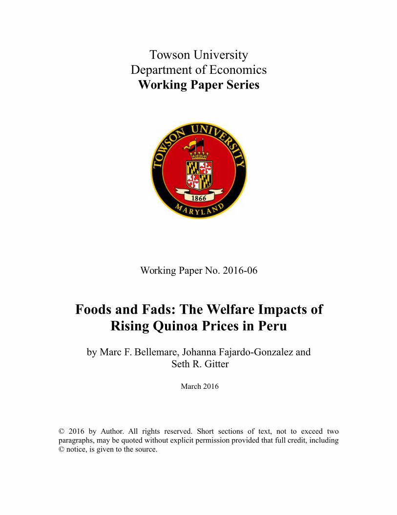
4.2. The Welfare Effects of Rising Quinoa Prices on Producers

Tables 5 to 7 present estimation results for our analysis the welfare impacts of rising quinoa prices for

quinoa producers. The main takeaway from that part of our empirical analysis is that higher levels of

quinoa production were associated with faster growth in household welfare, but only in 2013, i.e., at the

21

height of the quinoa price boom. This result is based on the interaction terms between year fixed effects

and the proportion of quinoa producers in a geographical unit, and it is robust to a number of different

specifications. Similarly, we find that higher levels of quinoa production are associated with less variable

levels of household welfare, but only in 2012-2013. This result is less robust than the result for welfare

levels.

The results from our core specification, shown in Table 5, are robust across at all three geographical

units of analysis, i.e., district (Table 5a), province (Table 5b), and department (Table 5c) for the 2013

results. Taking the first column of Table 5a as an example, the interpretation of the coefficient in the

first line is as follows: Relative to baseline household welfare, a district where 10 percent of households

were quinoa producers would have seen 2.94 percent more growth in welfare than a district without

any quinoa producers over the period 2004-2013. For reference, the average percentage of producers

was roughly 10 percent in districts that consumed quinoa. The magnitude of this coefficient is similar to

the one found in the previous regressions. Another way to interpret this is that a district where every

household produces quinoa would see its welfare grow 29.4 percent faster than a district where no

household produces quinoa. This is consistent with the evolution of welfare plotted in Figure 1, as well

as with the descriptive statistics in Table 1.

With that said, as the size of the geographical unit of observation increases, from district to province

(Tables 5a to 5b), and then from province to department (Tables 5b to 5c), we find that the size of the

point estimate on the 2013 interaction with quinoa production increases as the size of the geographical

unit of observation also increases. A comparison of the average number of quinoa producers given that

the region produces quinoa may help explain some of these differences in the point estimates. For

departments that produce quinoa the average percentage of households that were producers was 6

percent, while it is 16 percent and 29 percent for province and districts that have any quinoa

production. This increase in the point estimate as the geographical units get smaller is not surprising as

22

quinoa producing departments contain provinces or districts that do not produce quinoa. To compare

the coefficient on the main interaction (2013 x Proportion of Quinoa Producer) across geographic units

we could compare effects size given these average percentage of producers. The average quinoa

producing department, using column (1) of table 5c, would see an increase of consumption through the

interaction term of roughly 5.1 percent, which is the product of 6 percent and the point estimate 0.858.

Similarly, using columns (1) of 5b and 5c, the estimates suggest that the average quinoa producing

provinces and districts would see increases in consumption equivalent to 6.5 percent and 8.4 percent,

respectively.16 Additionally, the decreasing statistical power is consistent with there being less classical

measurement error the more observations go into making the relevant averages, and so with there

being less attenuation bias. The downside of considering larger geographical units, as we mentioned

earlier, is that the precision of our estimates declines as the size of the geographical unit of observation,

given the reduction in statistical power as the number of observations falls.

In some sense it may be surprising that the welfare of quinoa producers grew faster than that of the

average Peruvian households only in 2013 despite rising quinoa prices over the entire study period. A

closer look at the quinoa revenue data in table 3, however, shows stagnant revenue around 200 PEN

from quinoa sales for the period 2005-2008. The period 2009-2011 saw average revenues of around 400

PEN. In 2012, revenue jumped to 833 PEN, and it jumped further still to 912 PEN in 2013 due to

increased production per household. The 739-PEN change in quinoa revenue from 2004 to 2013

represents roughly 11 percent of baseline household consumption for those households. In other words,

the direct effect of quinoa revenue represents roughly one quarter of the total change of household

consumption during the time period. These results are robust to whether we exclude quinoa purchases

16 At the district level, the point estimate for 2013 is equal to 0.294, and there were on average 29% quinoa growers in districts that grew quinoa, so 0.085 = 0.294 x 0.29. Similarly, for provinces, the point estimate is equal to 0.407, and the average proportion of quinoa growers is 0.16, so 0.065 = 0.407 x 0.16.,

23

from the value of total household consumption, as in Tables 5a to 5c, or to whether we include them, as

in Appendix Table A1.

Tables 6a to 6c estimates specifications that are similar to those in Tables 5a to 5c, with a few

important exceptions. First, rather than treating the geographical unit as a unit of observation, the

results in Tables 6a to 6c treat the household as our unit of observation. Tables 6a to 6c respectively

control for district, province, and department fixed effects. Finally, columns 2 and 4 of Tables 6a to 6c

control for the date at which the household was surveyed, in order to control for seasonality, whereas

columns 1 and 3 do not. The very small difference between the results in columns 1 and 2 and between

those in columns 3 and 4 suggest that our results are not driven by seasonality. That being said, the

results in Tables 6a to 6c echo those in Tables 5a to 5c, that is: higher levels of quinoa production are

associated with faster growth in household welfare, but only in 2013, at the height of the quinoa price

boom.

Appendix Table A2 shows results that are similar to those in Tables 5a to 5c, with one important

exception: Rather than relying on the proportion of quinoa producers in a geographical unit in a given

year as treatment variable, those rely instead on the proportion of quinoa producers in a geographical

unit in 2004 as treatment variable. The results in Appendix Table A2 indicate that our core results are

robust to controlling for initial (i.e., 2004) conditions, in an effort to mitigate the potential reverse

causality issue due to households getting into quinoa production as a result of rising quinoa prices.

These results are robust to whether we exclude quinoa purchases from the value of total household

consumption, as in Appendix Table A2, or to whether we include them, as in Appendix Table A3.

Finally, in Tables 7a to 7c, we test for effects of quinoa production on the within-geographical unit

variability of welfare. Specifically, we examine the mean sum of squared differences between household

and (geographical unit-level) mean household consumption. In general, quinoa production is associated

24

with decreased variance over time. At the district level, in 2007 and 2012, the variance of household

welfare was 16 percent and 18 percent less for a community where everyone produced quinoa

compared to baseline non-quinoa growing communities. The 2012 result is robust across region size,

when going from Table 7a to 7b and from Table 7b to 7c, but the 2007 result is not.

5. Summary and Concluding Remarks

We have looked at whether the sharp rise in the price of quinoa over the period 2004-2013 has had any

impact on the welfare of quinoa consumers and producers in Peru. On the demand side, we find that an

increase in the purchase price of quinoa translates into positive general equilibrium effects on the

welfare of consumers. Specifically, a 1-percent increase in the purchase price of quinoa is associated

with a 0.07 percent increase in the welfare of quinoa-consuming households. On the supply side, we

find evidence that the rising price of quinoa has had a positive effect, both direct and indirect, on the

welfare of producer households. The direct effects operate through a faster increase in the rate of

welfare growth for households that produced quinoa relative to households that did not, but only in

2013, when quinoa prices were at their highest. The indirect effects operate through a reduction in the

variability of welfare for households that produced quinoa. Thus, it looks as though rising quinoa prices

have had first- as well as second-order welfare effects on quinoa producers.

The findings in this article are important for several reasons. First, Peruvian quinoa producers are

particularly poor, with an average consumption that is still only about half of that of households that do

not produce any quinoa. Recall that in 2013, some people advocated that consumers in rich countries

feel guilty about and reduced their consumption of quinoa because the rising international demand for

quinoa was hurting those who had traditionally produced and consumed it. It is useful to know that the

claim that rising quinoa prices were hurting those who had traditionally produced and consumed it—

those households in our sample that produce quinoa—was patently false. Second, the positive general

25

equilibrium effects of rising quinoa prices we identify for those households that consume quinoa are

interesting in and of themselves. Indeed, though Deaton’s (1989) short-term, partial-equilibrium

measure of the welfare impacts of an increase in the price of a commodity would suggest that quinoa

consumers would be hurt by rising quinoa prices, our longer-term, general-equilibrium estimates show

that for a 1-percent increase in the price of quinoa, household welfare increases by a modest 0.07

percent. These findings should assuage rich-country consumers’ concerns about whether their growing

demand for quinoa is having a negative influence on Andean households.

Early 2014 represented a peak for quinoa prices as international price data show that quinoa prices

began a precipitous decline in February of 2014. In fact, one might say that international prices have

declined as sharply between early 2014 and late 2015 as they have risen only a few years prior. By the

fourth quarter of 2015, the international price of quinoa had returned to its 2012 level. What is unclear

is how international price drops have influenced prices within Peru, and future research should address

whether falling prices have reduced consumption to pre-boom levels for quinoa-producing households.

With that said, our analysis raises important questions for future research that are well beyond the

scope of this article. For example, what about the indirect effects of rising quinoa prices? These could

include nutritional and health outcomes,17 agricultural wages, technology adoption, or educational

outcomes. Second, though quinoa producers tend to be poorer, our analysis does get into the

distributional effects of rising quinoa prices, nor do they look at changes in poverty rates. For now, we

leave these questions to future research.

17 Stevens (2015) looks at whether the quinoa price boom has affected nutritional outcomes in the Peruvian regions where quinoa has traditionally been consumed and finds no negative effects of rising quinoa prices on nutrition.

26

References

Andina (2016), “Peru: Agro-exports exceeded US$5.20 billion in 2015,” last accessed 3/3/2016 http://

www.andina.com.pe/Ingles/noticia-peru-agroexports-exceeded-520-billion-in-2015-597855.aspx

Angrist, Joshua, and Jörn-Steffen Pischke (2009), Mostly Harmless Econometrics, Princeton, NJ:

Princeton University Press.

Antman, Francisca, and David McKenzie (2007a), “Poverty Traps and Nonlinear Income Dynamics with

Measurement Error and Individual Heterogeneity,” Journal of Development Studies 43(6): 1057-

1083.

Antman, Francisca, and David McKenzie (2007b), “Earnings Mobility and Measurement Error: A Pseudo-

Panel Approach,” Economic Development and Cultural Change 56(1): 125-161.

Aragon, Fernando M., and Juan Pablo Rud (2013), “Natural Resources and Local Communities: Evidence

from a Peruvian Gold Mine,” American Economic Journal: Economic Policy 5(2): 1-25.

Barrett, Christopher B., and Paul Dorosh (1996), “Farmers' Welfare and Changing Food Prices:

Nonparametric Evidence from Rice in Madagascar,” American Journal of Agricultural Economics

78(3): 656-669.

Bellemare, Marc F., Christopher B. Barrett, and David R. Just (2013), “The Welfare Impacts of

Commodity Price Volatility: Evidence from Rural Ethiopia,” American Journal of Agricultural

Economics 95(4): 877-899.

Bertrand, Marianne, Esther Duflo, and Sendhil Mullainathan (2004), “How Much Should We Trust

Differences-in-Differences Estimates?,” Quarterly Journal of Economics 119(1): 249-275.

27

http://www.andina.com.pe/Ingles/noticia-peru-agroexports-exceeded-520-billion-in-2015-597855.aspx

Blythman, Johanna (2013), “Can Vegans Stomach the Unpalatable Truth about Quinoa?,” The Guardian,

http://www.theguardian.com/commentisfree/2013/jan/16/vegans-stomach-unpalatable-truth-

quinoa last accessed October 19, 2014.

Christiaensen, Luc J., and Kalanidhi Subbarao (2005), “Towards an Understanding of Household

Vulnerability in Rural Kenya,” Journal of African Economies 14(4): 520-558.

Cogneau, Denis, and Rémi Jedwab (2012), “Commodity Price Shocks and Child Outcomes: The 1990

Cocoa Crisis in Côte d’Ivoire,” Economic Development and Cultural Change 60(3): 507-534.

Cruces, Guillermo, Peter Lanjouw, Leonardo Lucchetti, Elizaveta Perova, Renos Vakis, and Mariana

Viollaz (2015), “Estimating Poverty Transitions Using Repeated Cross-Sections: A Three-Country

Validation Exercise,” Journal of Economic Inequality 13(2): 161-179.

Cuesta, Jose, Hugo Ñopo, and Georgina Pizzolitto (2011). “Using Pseudo-Panels to Measure Income

Mobility In Latin America,” Review of Income and Wealth 57(2): 224-246.

Deaton, Angus (1985), “Panel Data from Times Series of Cross-Sections,” Journal of Econometrics (30):

109-126.

Deaton, Angus (1989), “Household Survey Data and Pricing Policies in Developing Countries,” World

Bank Economic Review 3(2): 183-210.

Deaton, Angus (1997), The Analysis of Household Surveys, Baltimore, MD: Johns Hopkins University

Press.

Dell, Melissa (2010), “The Persistent Effects of Peru’s Mining Mita,” Econometrica 78(6): 1863-1903.

DePillis, Lydia (2013), “Quinoa Should Be Taking Over the World. This Is Why It Isn’t,” Washington Post,

July 11.

28

http://www.theguardian.com/commentisfree/2013/jan/16/vegans-stomach-unpalatable-truth-quinoa

http://www.theguardian.com/commentisfree/2013/jan/16/vegans-stomach-unpalatable-truth-quinoa

Dube, Oeindrila, and Juan F. Vargas (2013), “Commodity Price Shocks and Civil Conflict: Evidence from

Colombia,” Review of Economic Studies 80(4): 1384-1421.

Galdo, Jose (2013), “The Long-Run Labor-Market Consequences of Civil War: Evidence from the Shining

Path in Peru,” Economic Development and Cultural Change 61(4): 789-923.

Ivanic, Maros, and Will Martin (2008), “Implications of Higher Global Food Prices for Poverty in Low-

Income Countries,” Agricultural Economics 39(s1): 405-416.

McKenzie, David (2004), “Asymptotic Theory for Heterogeneous Dynamic Pseudo-Panels,” Journal of

Econometrics 120(2): 235-262.

Oxford English Dictionary (2014), “Superfood,”

http://www.oed.com/view/Entry/194186?redirectedFrom=superfood#eid69476470 last accessed

October 8, 2015.

Saunders, Doug (2013), “Killer Quinoa? Time to Debunk These Urban Food Myths,” The Globe and Mail,

http://www.theglobeandmail.com/globe-debate/chow-down-on-quinoa-and-three-modern-food-

fallacies/article7536845/ last accessed October 19, 2014.

Stevens, Andrew (2015), “Quinoa Quandary: Cultural Tastes and Nutrition in Peru,” Working Paper,

University of California—Berkeley.

Wodon, Quentin, and Hassan Zaman (2010), “Higher Food Prices in Sub-Saharan Africa: Poverty Impact

and Policy Responses,” World Bank Research Observer 25(1): 157-176.

Wooldridge, Jeffrey M. (2002), Econometric Analysis of Cross Section and Panel Data, Cambridge, MA:

MIT Press.

29

http://www.oed.com/view/Entry/194186?redirectedFrom=superfood%23eid69476470

http://www.theglobeandmail.com/globe-debate/chow-down-on-quinoa-and-three-modern-food-fallacies/article7536845/

http://www.theglobeandmail.com/globe-debate/chow-down-on-quinoa-and-three-modern-food-fallacies/article7536845/

Zezza, Alberto, Benjamin Davis, Carlo Azzarri, Katia Covarrubias, Luca Tasciotti, and Gustavo Anriquez

(2008), “The Impact of Rising Food Prices on the Poor”, Working Paper, Food and Agricultural

Organization of the United Nations, Rome: Italy.

30

Figure 1. Ratio of Total Current Consumption to Baseline Consumption, Excluding Quinoa Consumption.

31

Table 1. Household Welfare Trends in Constant Terms, 2004-2013.

Year

Household Consumption in 2004 PEN

Non-Consumers and Non-

Producers of Quinoa

Producer of Quinoa

Non-Producer Consumers of Quinoa

2004 11,930 6,264 16,471 2005 11,372 6,097 16,314 2006 12,365 6,294 17,736 2007 13,163 6,536 18,643 2008 13,550 6,907 18,598 2009 14,137 7,367 19,965 2010 14,640 7,818 19,977 2011 14,761 8,270 19,733 2012 15,224 8,121 20,345 2013 15,316 9,134 21,611

Note: Figures measured in 2004 PEN and exclude consumption of cultivated and purchased quinoa. All descriptive statistics are weighted using the sampling weights provided in the ENAHO. In addition to being expressed in constant (i.e., 2004) terms, all prices are deflated using departmental-level deflators.

32

Table 2. Descriptive Statistics for Quinoa Consumers, 2004-2013.

Year Proportion of

Quinoa-Consuming Households (%)

Kg of Whole Quinoa Purchased,

Past 2 Weeks

Purchase Price of Whole Quinoa Per

Kg, 2004 PEN

Budget Share of Annual Total

Consumption of Quinoa, All

Households (%) 2004 26.8% 0.87 3.15 0.10% 2005 30.7% 0.79 3.28 0.12% 2006 30. 6% 0.83 3.14 0.11% 2007 29.6% 0.82 3.25 0.11% 2008 25.7% 0.74 4.36 0.53% 2009 24.6% 0.67 6.25 0.56% 2010 25.8% 0.72 6.44 0.54% 2011 27.9% 0.74 6.36 0.56% 2012 29.4% 0.7 6.31 0.57% 2013 30.8% 0.68 7.83 0.63%

Note: Average purchase amount for households who purchased quinoa. In addition to being expressed in constant (i.e., 2004) terms, all prices are deflated using annual departmental-level deflators. Budget shares are imputed by multiplying the value of purchases in the previous two weeks by 26 and dividing by total household consumption.

33

Table 3. Descriptive Statistics for Quinoa Producers, 2004-2013.

Year

Sample Proportion of

Quinoa Producers (%)

Sample Proportion of Quinoa Sellers (%)

Quinoa Production,

Past 12 Months (Kg), Quinoa

Producers Only

Own Consumption (%), Quinoa Producers

Only

Average Sales

Price (Per Kg, 2004

PEN)

Quinoa Revenue (Quinoa

Sellers Only, 2004 PEN)

Quinoa Revenue

(All Quinoa Farmers,

2004 PEN) 2004 3.69% 0.30% 69 73% 1.34 154 12 2005 3.92% 0.42% 63 63% 1.61 232 24 2006 3.90% 0.37% 71 66% 1.68 199 19 2007 3.69% 0.31% 56 54% 1.55 117 9 2008 3.06% 0.20% 40 56% 2.23 244 14 2009 3.38% 0.30% 49 49% 3.95 462 38 2010 3.56% 0.29% 52 52% 3.64 375 28 2011 3.38% 0.50% 71 40% 3.83 448 58 2012 2.81% 0.46% 87 33% 4.44 813 125 2013 2.63% 0.46% 76 34% 6.17 1035 171

Note: All descriptive statistics are weighted using the sampling weights provided in the ENAHO. In addition to being expressed in constant (i.e., 2004) terms, all prices are deflated using departmental-level deflators.

34

Table 4a. Pseudo-Panel Regression of Total Household Consumption on the Price of Quinoa Treating Districts as Units of Observation for the Period 2004-2013.

Variables (1) (2) (3) (4) (5) (6) (7) Dependent Variable: Log of Total Value of Household Consumption.

Log of Price of Quinoa 0.082*** 0.047** 0.066*** 0.066*** 0.024 0.077*** 0.049** (0.017) (0.021) (0.018) (0.017) (0.024) (0.016) (0.022)

Constant -46.380*** 8.983*** 8.905*** -51.807*** 9.012*** -46.530*** 8.983*** (4.710) (0.026) (0.016) (4.335) (0.027) (4.569) (0.027)

Observations 5,232 5,232 5,232 5,232 5,232 5,232 5,232 District Fixed Effects Yes Yes Yes Yes Yes Yes Yes Linear Trend Yes No No No No No No Year Fixed Effects No Yes No No No No No District-Specific Trends No No Yes No No No No Province-Specific Trends No No No Yes No No No Province-Year Fixed Effects No No No No Yes No No Department-Specific Trends No No No No No Yes No Department-Year Fixed Effects No No No No No No Yes R-squared 0.190 0.195 0.510 0.295 0.550 0.233 0.296

Note: *, **, and *** denote statistical significance at the 10, 5, and 1 percent levels, respectively. The sample only includes district-year observations where quinoa was consumed. Standard errors clustered at the district level are shown in parentheses. Each household is weighted according to the sampling weight it was given in the ENAHO. In addition to being expressed in constant (i.e., 2004) terms, all prices are deflated using departmental-level deflators.

35

Table 4b. Pseudo-Panel Regression of Total Household Consumption on the Price of Quinoa Treating Provinces as the Units of Observation. Variables (1) (2) (3) (4) (5)

Dependent Variable: Log of Total Value of Household Consumption Log of Price of Quinoa 0.110*** 0.090*** 0.092*** 0.115*** 0.120***

(0.023) (0.033) (0.025) (0.023) (0.036) Constant -52.621*** 8.768*** 8.705*** -49.746*** 8.742***

(6.234) (0.040) (0.021) (5.949) (0.040)

Observations 1,590 1,590 1,590 1,590 1,590 Province Fixed Effects Yes Yes Yes Yes Yes Linear Trend Yes No No No No Year Fixed Effects No Yes No No No Province-Specific Linear Trends No No Yes No No Department-Specific Linear Trends No No No Yes No Department-Year Fixed Effects No No No No Yes R-squared 0.386 0.396 0.620 0.461 0.553

Note: *, **, and *** denote statistical significance at the 10, 5, and 1 percent levels, respectively. The sample only includes province-year observations where quinoa was consumed. Standard errors clustered at the province level are shown in parentheses. Each household is weighted according to the sampling weight it was given in the ENAHO. In addition to being expressed in constant (i.e., 2004) terms, all prices are deflated using departmental-level deflators.

36

Table 4c. Pseudo-Panel Regression of Total Household Consumption on the Price of Quinoa Treating Departments as the Units of Observation.

Variables (1) (2) (3) Dependent Variable: Log of Total Value of Household Consumption

Log of Price of Quinoa 0.079** 0.072 0.066** (0.037) (0.094) (0.030)

Constant -55.711*** 9.018*** -61.265*** (9.780) (0.110) (4.219)

Observations 1,590 1,590 1,590 Department Fixed Effects Yes Yes Yes Linear Trend Yes No No Year Fixed Effects No Yes No Department-Specific Linear Trends No No Yes R-squared 0.674 0.692 0.854

Note: *, **, and *** denote statistical significance at the 10, 5, and 1 percent levels, respectively. The sample only includes department-year observations where quinoa was consumed. Standard errors clustered at the department level are shown in parentheses. Each household is weighted according to the sampling weight it was given in the ENAHO. In addition to being expressed in constant (i.e., 2004) terms, all prices are deflated using departmental-level deflators.

37

Table 5a. Pseudo-Panel Regression of the Average Log of Total Household Consumption (Excluding Quinoa Consumption) on the Proportion of Households Who Produce Quinoa Treating Districts as Units of Observations, 2004-2013.

Variable

All Districts Quinoa-Producing Districts

Quinoa-Consuming

Districts

Districts with Quinoa

Consumption above the Mean

Dependent Variable: Log of Total Household Consumption (in 2004 PEN). 2013*Proportion of Quinoa Producers 0.294*** 0.244* 0.358*** 0.344***

(0.090) (0.126) (0.091) (0.094) 2012*Proportion of Quinoa Producers 0.079 -0.021 0.104 0.164*

(0.085) (0.118) (0.087) (0.091) 2011*Proportion of Quinoa Producers -0.034 0.014 0.034 0.073

(0.090) (0.126) (0.092) (0.098) 2010*Proportion of Quinoa Producers 0.009 0.005 0.043 0.089





(0.084) (0.123) (0.088) (0.095) 2005*Proportion of Quinoa Producers -0.163* -0.361*** -0.160* -0.141

(0.084) (0.128) (0.089) (0.095) 2013 Dummy 0.302*** 0.318*** 0.273*** 0.273***

(0.015) (0.050) (0.017) (0.024) 2012 Dummy 0.268*** 0.319*** 0.254*** 0.223***

(0.016) (0.049) (0.018) (0.024) 2011 Dummy 0.248*** 0.230*** 0.218*** 0.206***

(0.016) (0.052) (0.018) (0.025)

38

2010 Dummy 0.214*** 0.219*** 0.201*** 0.175*** (0.016) (0.053) (0.018) (0.024)

2009 Dummy 0.145*** 0.130** 0.150*** 0.165*** (0.017) (0.053) (0.019) (0.025)

2008 Dummy 0.094*** 0.022 0.086*** 0.071*** (0.016) (0.054) (0.018) (0.025)

2007 Dummy 0.055*** 0.021 0.041** 0.039 (0.016) (0.051) (0.018) (0.025)

2006 Dummy 0.033*** 0.020 0.038** 0.029 (0.012) (0.047) (0.015) (0.021)

2005 Dummy -0.023** 0.074 -0.021 -0.024 (0.012) (0.048) (0.016) (0.021)

Proportion of Quinoa Producers 0.097 0.062 0.020 -0.046 (0.079) (0.105) (0.082) (0.088)

Constant 8.782*** 8.439*** 8.870*** 8.883*** (0.012) (0.041) (0.014) (0.019)

Observations 9,613 2,360 6,922 4,180 District Fixed Effects Yes Yes Yes Yes R-squared 0.171 0.187 0.175 0.176 Number of Districts 1,401 554 1,233 937

Note: *, **, and *** denote statistical significance at the 10, 5, and 1 percent levels, respectively. Clustered standard errors in parentheses; clustering is at the district level. Each household is weighted according to the sampling weights given in the ENAHO. In addition to being expressed in constant (i.e., 2004) terms, all prices are deflated using departmental-level deflators.

39

Table 5b. Pseudo-Panel Regression of the Average Log of Total Household Consumption (Excluding Quinoa Consumption) on the Proportion of Households Who Produce Quinoa Treating Provinces as Units of Observation, 2004-2013.

Variable

All Provinces Quinoa-Producing Provinces

Quinoa-Consuming Provinces

Provinces with Quinoa


Dependent Variable: Log of Total Household Consumption (in 2004 PEN). 2013*Proportion of Quinoa Producers 0.407** 0.169 0.461*** 0.495***

(0.161) (0.192) (0.156) (0.175) 2012*Proportion of Quinoa Producers 0.133 -0.094 0.163 0.297*

(0.147) (0.176) (0.142) (0.164) 2011*Proportion of Quinoa Producers -0.050 -0.131 -0.012 0.109

(0.144) (0.180) (0.139) (0.158) 2010*Proportion of Quinoa Producers 0.004 -0.167 -0.037 0.104

(0.162) (0.194) (0.155) (0.181) 2009*Proportion of Quinoa Producers 0.048 -0.225 -0.010 -0.028

(0.164) (0.193) (0.156) (0.182) 2008*Proportion of Quinoa Producers -0.012 -0.047 -0.015 0.092



(0.105) (0.140) (0.106) (0.119) 2005*Proportion of Quinoa Producers -0.113 -0.210 -0.116 -0.172

(0.128) (0.159) (0.130) (0.147) 2013 Dummy 0.300*** 0.361*** 0.286*** 0.265***

(0.025) (0.040) (0.024) (0.035) 2012 Dummy 0.279*** 0.339*** 0.271*** 0.223***

(0.025) (0.042) (0.024) (0.037) 2011 Dummy 0.275*** 0.298*** 0.263*** 0.234***

(0.025) (0.044) (0.023) (0.035)

40

2010 Dummy 0.220*** 0.280*** 0.233*** 0.198*** (0.026) (0.041) (0.023) (0.037)

2009 Dummy 0.156*** 0.237*** 0.175*** 0.182*** (0.028) (0.041) (0.024) (0.040)

2008 Dummy 0.128*** 0.137*** 0.131*** 0.100*** (0.025) (0.043) (0.023) (0.038)

2007 Dummy 0.058** 0.062 0.055** 0.029 (0.026) (0.039) (0.023) (0.035)

2006 Dummy 0.026 0.023 0.022 0.036 (0.017) (0.038) (0.019) (0.029)

2005 Dummy -0.025 0.003 -0.023 0.008 (0.016) (0.035) (0.018) (0.033)

Proportion of Quinoa Producers -0.134 -0.119 -0.150 -0.344** (0.160) (0.175) (0.158) (0.171)

Constant 8.824*** 8.606*** 8.837*** 8.869*** (0.019) (0.033) (0.018) (0.028)

Observations 1,919 851 1,750 852 Province Fixed Effects Yes Yes Yes Yes R-squared 0.345 0.412 0.374 0.381 Number of Provinces 194 115 193 130

Note: *, **, and *** denote statistical significance at the 10, 5, and 1 percent levels, respectively. Clustered standard errors in parentheses; clustering is at the provincial level. Each household is weighted according to the sampling weights given in the ENAHO. In addition to being expressed in constant (i.e., 2004) terms, all prices are deflated using departmental-level deflators.

41

Table 5c. Pseudo-Panel Regression of the Average Log of Total Household Consumption (Excluding Quinoa Consumption) on the Proportion of Households Who Produce Quinoa Treating Departments as Units of Observation, 2004-2013.

Variable

All Departments Quinoa-Producing Departments

Departments with Quinoa


Dependent Variable: Log of Total Household Consumption (in 2004 PEN). 2013*Proportion of Quinoa Producers 0.858* 0.772* 0.706**

(0.461) (0.433) (0.299) 2012*Proportion of Quinoa Producers 0.330 0.206 0.329



(0.231) (0.311) (0.246) 2009*Proportion of Quinoa Producers 0.160 0.015 -0.010




(0.207) (0.250) (0.334) 2005*Proportion of Quinoa Producers -0.116 -0.221 -0.238

(0.130) (0.176) (0.220) 2013 Dummy 0.270*** 0.286*** 0.253***

(0.033) (0.044) (0.036) 2012 Dummy 0.283*** 0.305*** 0.250***

(0.034) (0.055) (0.034) 2011 Dummy 0.252*** 0.278*** 0.217***

(0.029) (0.047) (0.028)

42

2010 Dummy 0.232*** 0.265*** 0.222*** (0.024) (0.042) (0.032)

2009 Dummy 0.174*** 0.200*** 0.191*** (0.023) (0.035) (0.033)

2008 Dummy 0.120*** 0.133*** 0.124*** (0.025) (0.027) (0.032)

2007 Dummy 0.077*** 0.094*** 0.095** (0.020) (0.027) (0.037)

2006 Dummy 0.033* 0.039 0.078** (0.018) (0.028) (0.032)

2005 Dummy -0.018 0.001 0.021 (0.018) (0.029) (0.033)

Proportion of Quinoa Producers -0.584 -0.497 -1.027 (0.889) (0.946) (0.634)

Constant 9.123*** 8.938*** 9.168*** (0.044) (0.077) (0.045)

Observations 250 145 131 Department Fixed Effects Yes Yes Yes R-squared 0.708 0.712 0.787 Number of Departments 25 18 17

Note: *, **, and *** denote statistical significance at the 10, 5, and 1 percent levels, respectively. Clustered standard errors in parentheses; clustering is at the departmental level. Each household is weighted according to the sampling weights given in the ENAHO. Because all departments consume quinoa, there are no specifications for quinoa-consuming departments only. In addition to being expressed in constant (i.e., 2004) terms, all prices are deflated using departmental-level deflators.

43

Table 6a. Household-Level Regression of Total Household Consumption (Excluding Quinoa Consumption) on whether the Household Produced Quinoa, 2004-2013.

Variables All

Districts All

Districts

Quinoa-Producing Districts

Only

Quinoa-Producing Districts

Only Dependent Variable: Log of Total Household Consumption (in 2004 PEN).

2013*HH Quinoa Producer Dummy 0.172*** 0.174*** 0.117** 0.121** (0.048) (0.049) (0.047) (0.048)

2012*HH Quinoa Producer Dummy 0.079* 0.079* 0.055 0.061 (0.043) (0.043) (0.044) (0.045)

2011*HH Quinoa Producer Dummy 0.080* 0.080* 0.090* 0.094* (0.043) (0.043) (0.048) (0.048)

2010*HH Quinoa Producer Dummy 0.071 0.071 0.053 0.057 (0.046) (0.046) (0.048) (0.048)


2008*HH Quinoa Producer Dummy 0.056 0.056 0.083 0.087* (0.049) (0.049) (0.051) (0.051)


2006*HH Quinoa Producer Dummy -0.024 -0.023 -0.038 -0.037 (0.045) (0.045) (0.047) (0.047)


2013 Dummy 0.282*** 0.282*** 0.333*** 0.333*** (0.013) (0.013) (0.034) (0.033)

2012 Dummy 0.258*** 0.257*** 0.280*** 0.280*** (0.013) (0.013) (0.031) (0.031)

2011 Dummy 0.227*** 0.227*** 0.216*** 0.216*** (0.013) (0.013) (0.034) (0.033)

44

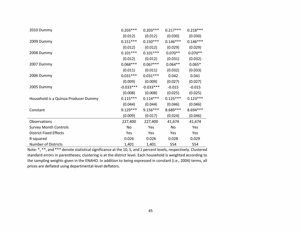
2010 Dummy 0.203*** 0.203*** 0.217*** 0.218*** (0.012) (0.012) (0.030) (0.030)

2009 Dummy 0.151*** 0.150*** 0.146*** 0.146*** (0.012) (0.012) (0.029) (0.029)

2008 Dummy 0.101*** 0.101*** 0.070** 0.070** (0.012) (0.012) (0.031) (0.032)

2007 Dummy 0.068*** 0.067*** 0.064** 0.065* (0.011) (0.011) (0.032) (0.033)

2006 Dummy 0.031*** 0.031*** 0.042 0.041 (0.009) (0.009) (0.027) (0.027)

2005 Dummy -0.033*** -0.033*** -0.015 -0.015 (0.008) (0.008) (0.025) (0.025)

Household is a Quinoa Producer Dummy 0.115*** 0.114*** 0.125*** 0.123*** (0.044) (0.044) (0.046) (0.046)

Constant 9.129*** 9.156*** 8.689*** 8.694*** (0.009) (0.017) (0.024) (0.046)

Observations 227,400 227,400 41,674 41,674 Survey Month Controls No Yes No Yes District Fixed Effects Yes Yes Yes Yes R-squared 0.026 0.026 0.028 0.029 Number of Districts 1,401 1,401 554 554


45

Table 6b. Household-Level Regression of Total Household Consumption (Excluding Quinoa Consumption) on whether the Household Produced Quinoa, 2004-2013.

Variable All

Provinces All

Provinces

Quinoa-Producing Provinces

Only

Quinoa-Producing Provinces

Only Dependent Variable: Log of Total Household Consumption (in 2004 PEN).

2013*HH Quinoa Producer Dummy 0.142*** 0.141*** 0.109** 0.108** (0.054) (0.054) (0.052) (0.053)









2013 Dummy 0.287*** 0.287*** 0.319*** 0.318*** (0.016) (0.016) (0.025) (0.025)

2012 Dummy 0.264*** 0.265*** 0.283*** 0.282*** (0.017) (0.017) (0.029) (0.029)

2011 Dummy 0.233*** 0.233*** 0.223*** 0.222*** (0.016) (0.016) (0.029) (0.029)

46

2010 Dummy 0.217*** 0.217*** 0.221*** 0.220*** (0.015) (0.015) (0.025) (0.025)

2009 Dummy 0.165*** 0.165*** 0.169*** 0.168*** (0.015) (0.015) (0.026) (0.026)

2008 Dummy 0.117*** 0.117*** 0.086*** 0.086*** (0.015) (0.015) (0.023) (0.023)

2007 Dummy 0.085*** 0.085*** 0.055** 0.054** (0.013) (0.013) (0.022) (0.023)

2006 Dummy 0.030** 0.030** 0.041 0.041 (0.013) (0.013) (0.026) (0.026)

2005 Dummy -0.036*** -0.036*** -0.008 -0.008 (0.011) (0.011) (0.023) (0.023)

Household is a Quinoa Producer Dummy -0.036 -0.034 -0.033 -0.032 (0.071) (0.070) (0.070) (0.070)

Constant 9.128*** 9.152*** 8.816*** 8.837*** (0.010) (0.017) (0.019) (0.028)

Observations 227,400 227,400 76,839 76,839 Survey Month Controls No Yes No Yes Province Fixed Effects Yes Yes Yes Yes R-squared 0.024 0.024 0.021 0.022 Number of Provinces 194 194 115 115

Note: *, **, and *** denote statistical significance at the 10, 5, and 1 percent levels, respectively. Clustered standard errors in parentheses; clustering is at the provincial level. Each household is weighted according to the sampling weights given in the ENAHO. In addition to being expressed in constant (i.e., 2004) terms, all prices are deflated using departmental-level deflators.

47

Table 6c. Household-Level Regression of Total Household Consumption (Excluding Quinoa Consumption) on whether the Household Produced Quinoa, 2004-2013.

Variable All

Departments All

Departments

Quinoa-Producing

Departments Only

Quinoa-Producing

Departments Only

Dependent Variable: Log of Total Household Consumption (in 2004 PEN). 2013*HH Quinoa Producer Dummy 0.135** 0.135** 0.134** 0.131**

(0.057) (0.057) (0.051) (0.052) 2012*HH Quinoa Producer Dummy 0.042 0.040 0.049 0.046

(0.040) (0.039) (0.041) (0.040) 2011*HH Quinoa Producer Dummy 0.056 0.055 0.067** 0.066**




(0.052) (0.051) (0.044) (0.044) 2007*HH Quinoa Producer Dummy -0.021 -0.023 -0.005 -0.008

(0.060) (0.060) (0.053) (0.052) 2006*HH Quinoa Producer Dummy -0.042 -0.042 -0.052* -0.052*

(0.033) (0.033) (0.030) (0.029) 2005*HH Quinoa Producer Dummy -0.065 -0.063 -0.088 -0.087

(0.066) (0.066) (0.068) (0.069) 2013 Dummy 0.271*** 0.271*** 0.272*** 0.272***

(0.027) (0.027) (0.035) (0.035) 2012 Dummy 0.253*** 0.253*** 0.245*** 0.245***

(0.027) (0.027) (0.039) (0.039) 2011 Dummy 0.219*** 0.219*** 0.209*** 0.209***

(0.024) (0.024) (0.035) (0.035)

48

2010 Dummy 0.208*** 0.208*** 0.204*** 0.204*** (0.020) (0.020) (0.033) (0.033)

2009 Dummy 0.155*** 0.155*** 0.148*** 0.148*** (0.020) (0.020) (0.032) (0.032)

2008 Dummy 0.109*** 0.109*** 0.093*** 0.093*** (0.022) (0.022) (0.029) (0.029)

2007 Dummy 0.079*** 0.079*** 0.063** 0.063** (0.018) (0.018) (0.024) (0.024)

2006 Dummy 0.032* 0.032* 0.041* 0.041* (0.018) (0.018) (0.023) (0.023)

2005 Dummy -0.036** -0.036** -0.013 -0.013 (0.015) (0.015) (0.020) (0.020)

Household is a Quinoa Producer Dummy -0.239*** -0.237*** -0.242*** -0.240*** (0.073) (0.072) (0.069) (0.069)

Constant 9.144*** 9.157*** 8.965*** 8.966*** (0.015) (0.019) (0.021) (0.020)

Observations 227,400 227,400 128,666 128,666 Survey Month Controls No Yes No Yes Department Fixed Effects Yes Yes Yes Yes R-squared 0.022 0.022 0.020 0.021 Number of Departments 25 25 18 18

Note: *, **, and *** denote statistical significance at the 10, 5, and 1 percent levels, respectively. Clustered standard errors in parentheses; clustering is at the departmental level. Each household is weighted according to the sampling weights given in the ENAHO. In addition to being expressed in constant (i.e., 2004) terms, all prices are deflated using departmental-level deflators.

49

Table 7a. Pseudo-Panel Regression of the Variance of Total Household Consumption on the Percentage of Households Who Produce Quinoa Treating Districts as Units of Observation, 2004-2013.

Variables

All Districts

Quinoa-Growing Districts

Only

Quinoa-Consuming

Districts Only

Districts with Quinoa

Consumption above the

Mean Dependent Variable: Variance of Total Household Consumption.

2013*Proportion of Quinoa Producers -0.075 -0.058 -0.032 -0.047 (0.083) (0.127) (0.085) (0.090)

2012*Proportion of Quinoa Producers -0.175** -0.055 -0.114 -0.122 (0.081) (0.119) (0.083) (0.087)



2009*Proportion of Quinoa Producers -0.040 0.034 0.004 0.005 (0.086) (0.124) (0.089) (0.095)


2007*Proportion of Quinoa Producers -0.157** -0.122 -0.136* -0.165** (0.073) (0.108) (0.075) (0.079)

2006*Proportion of Quinoa Producers 0.017 0.150 0.063 0.055 (0.065) (0.113) (0.068) (0.074)

2005*Proportion of Quinoa Producers 0.024 0.094 0.079 0.078 (0.076) (0.120) (0.079) (0.085)

2013 Dummy 0.030*** 0.010 0.005 0.001 (0.010) (0.047) (0.012) (0.018)

2012 Dummy 0.038*** -0.023 0.007 -0.000 (0.010) (0.046) (0.013) (0.018)

2011 Dummy 0.045*** 0.065 0.023* 0.010 (0.011) (0.048) (0.013) (0.019)

2010 Dummy 0.031*** 0.006 0.008 0.014 (0.011) (0.045) (0.013) (0.020)

50

2009 Dummy 0.039*** 0.001 0.016 0.010 (0.011) (0.045) (0.014) (0.021)

2008 Dummy 0.044*** 0.043 0.025* 0.026 (0.011) (0.048) (0.013) (0.020)

2007 Dummy 0.026** 0.012 0.016 0.019 (0.011) (0.045) (0.014) (0.019)

2006 Dummy 0.016* -0.046 -0.004 -0.001 (0.010) (0.049) (0.013) (0.019)

2005 Dummy 0.009 -0.022 -0.017 -0.016 (0.009) (0.044) (0.012) (0.018)

Proportion of Quinoa Producers -0.017 -0.101 -0.052 -0.028 (0.069) (0.103) (0.071) (0.076)

Constant 0.369*** 0.495*** 0.404*** 0.413*** (0.008) (0.038) (0.010) (0.015)

Observations 9,613 2,360 6,922 4,180 District Fixed Effects Yes Yes Yes Yes R-squared 0.007 0.020 0.008 0.011 Number of Districts 1,401 554 1,233 937

Note: *, **, and *** denote statistical significance at the 10, 5, and 1 percent levels, respectively. Clustered standard errors in parentheses. Each household is weighted according to the sampling weights given in the ENAHO. In addition to being expressed in constant (i.e., 2004) terms, all prices are deflated using departmental-level deflators.

51

Table 7b. Pseudo-Panel Regression of the Variance of Total Household Consumption on the Percentage of Households Who Produce Quinoa Treating Provinces as Units of Observation, 2004-2013.

Variables

All Provinces

Quinoa-Growing

Provinces Only

Quinoa-Consuming Provinces

Only

Provinces with Quinoa Consumption

above the Mean

Dependent Variable: Variance of Total Household Consumption. 2013*Proportion of Quinoa Producers -0.196 -0.183 -0.128 -0.167

(0.122) (0.147) (0.123) (0.127) 2012*Proportion of Quinoa Producers -0.257** -0.270* -0.179 -0.223*

(0.120) (0.146) (0.119) (0.127) 2011*Proportion of Quinoa Producers -0.019 -0.057 0.038 -0.001





(0.115) (0.149) (0.115) (0.124) 2006*Proportion of Quinoa Producers 0.013 -0.040 0.049 0.035


(0.122) (0.159) (0.125) (0.145) 2013 Dummy 0.019 0.017 0.001 -0.007

(0.016) (0.036) (0.016) (0.027) 2012 Dummy 0.041** 0.046 0.019 0.016

(0.016) (0.034) (0.015) (0.025) 2011 Dummy 0.045*** 0.058 0.029* 0.018

(0.016) (0.036) (0.016) (0.027) 2010 Dummy 0.031* 0.017 0.013 -0.014

(0.016) (0.036) (0.016) (0.027)

52

2009 Dummy 0.050*** 0.036 0.033** 0.011 (0.016) (0.037) (0.016) (0.034)

2008 Dummy 0.054*** 0.087** 0.039** 0.027 (0.016) (0.037) (0.016) (0.029)

2007 Dummy 0.056*** 0.077* 0.047*** 0.057** (0.018) (0.039) (0.018) (0.028)

2006 Dummy 0.013 0.029 0.004 -0.007 (0.015) (0.037) (0.015) (0.028)

2005 Dummy 0.003 -0.014 -0.010 -0.001 (0.014) (0.033) (0.015) (0.028)

Proportion of Quinoa Producers 0.023 0.057 -0.015 0.057 (0.121) (0.141) (0.121) (0.127)

Constant 0.461*** 0.537*** 0.486*** 0.518*** (0.013) (0.030) (0.013) (0.023)

Observations 1,919 851 1,750 852 Province Fixed Effects Yes Yes Yes Yes R-squared 0.033 0.046 0.030 0.044 Number of Provinces 194 115 193 130

Note: *, **, and *** denote statistical significance at the 10, 5, and 1 percent levels, respectively. Clustered standard errors in parentheses. Each household is weighted according to the sampling weights given in the ENAHO. In addition to being expressed in constant (i.e., 2004) terms, all prices are deflated using departmental-level deflators.

53

Table 7c. Pseudo-Panel Regression of the Variance of Total Household Consumption on the Percentage of Households Who Produce Quinoa Treating Departments as Units of Observation, 2004-2013.

Variables

All Departments

Quinoa-Growing

Departments Only

Departments with Quinoa Consumption

above the Mean

Dependent Variable: Variance of Total Household Consumption. 2013*Proportion of Quinoa Producers -0.349** -0.534*** -0.383**

(0.149) (0.156) (0.154) 2012*Proportion of Quinoa Producers -0.331** -0.424*** -0.272**

(0.150) (0.120) (0.120) 2011*Proportion of Quinoa Producers 0.073 -0.054 0.044




(0.244) (0.233) (0.183) 2007*Proportion of Quinoa Producers -0.184 -0.350** -0.308**


(0.215) (0.189) (0.166) 2005*Proportion of Quinoa Producers 0.324* 0.297 0.281

(0.189) (0.183) (0.193) 2013 Dummy -0.043* -0.013 -0.048*

(0.021) (0.027) (0.024) 2012 Dummy -0.030 -0.013 -0.052**

(0.024) (0.026) (0.023) 2011 Dummy -0.034 -0.011 -0.046*

(0.020) (0.028) (0.026)

54

2010 Dummy -0.010 0.005 -0.028 (0.021) (0.032) (0.023)

2009 Dummy 0.011 0.018 -0.005 (0.023) (0.034) (0.030)

2008 Dummy 0.016 0.043 0.003 (0.019) (0.029) (0.022)

2007 Dummy 0.028 0.060** 0.029 (0.020) (0.022) (0.028)

2006 Dummy 0.009 0.026 -0.011 (0.019) (0.030) (0.026)

2005 Dummy -0.005 -0.002 -0.016 (0.013) (0.019) (0.020)

Proportion of Quinoa Producers -0.227 -0.129 0.048 (0.411) (0.382) (0.363)

Constant 0.565*** 0.632*** 0.604*** (0.017) (0.021) (0.024) Observations 250 145 131 Departmental Fixed Effects Yes Yes Yes R-squared 0.237 0.288 0.385 Number of Departments 25 18 17

Note: *, **, and *** denote statistical significance at the 10, 5, and 1 percent levels, respectively. Clustered standard errors in parentheses. Each household is weighted according to the sampling weights given in the ENAHO. Because all departments consume quinoa, there are no specifications for quinoa-consuming departments only. In addition to being expressed in constant (i.e., 2004) terms, all prices are deflated using departmental-level deflators.

55

Appendix Table A1. Robustness Check of the Pseudo-Panel Regression of the Average Log of Total Household Consumption (Including Quinoa Purchases) on the Proportion of Households Who Produce Quinoa Treating Districts, Provinces, and Departments as Units Observation, 2004-2013.

Variables All Districts All Provinces All Departments

Dependent Variable: Log of Total Household Consumption (in 2004 PEN). 2013*Proportion of Quinoa Producers 0.370*** 0.317** 0.876

(0.069) (0.130) (0.542) 2012*Proportion of Quinoa Producers 0.157** 0.044 0.271



(0.065) (0.131) (0.385) 2009*Proportion of Quinoa Producers 0.105* -0.046 0.049



(0.066) (0.111) (0.432) 2006*Proportion of Quinoa Producers 0.060 -0.019 -0.011


(0.073) (0.127) (0.293) 2013 Dummy 0.297*** 0.306*** 0.275***

(0.015) (0.024) (0.032) 2012 Dummy 0.263*** 0.285*** 0.289***

(0.016) (0.024) (0.031)

56

2011 Dummy 0.243*** 0.281*** 0.258*** (0.016) (0.023) (0.026)

2010 Dummy 0.209*** 0.226*** 0.236*** (0.016) (0.025) (0.022)

2009 Dummy 0.140*** 0.162*** 0.178*** (0.016) (0.026) (0.022)

2008 Dummy 0.089*** 0.134*** 0.125*** (0.016) (0.024) (0.025)

2007 Dummy 0.051*** 0.064** 0.083*** (0.016) (0.025) (0.021)

2006 Dummy 0.029** 0.032* 0.039* (0.012) (0.017) (0.020)

2005 Dummy -0.028** -0.019 -0.012 (0.011) (0.017) (0.021)

Constant 8.789*** 8.817*** 9.101*** (0.011) (0.016) (0.017)

Observations 9,613 1,919 250 R-squared 0.171 0.345 0.706 District Fixed Effects Yes No No Provincial Fixed Effects Yes Yes No Departmental Fixed Effects Yes Yes Yes


57

Table A2. Robustness Check of the Pseudo-Panel Regression of the Average Log of Total Household Consumption (Excluding Quinoa Consumption) on the Proportion of Households Who Produced Quinoa in 2004 Treating Districts, Provinces, and Departments as Units of Observation, 2004-2013.

Variables All Districts All Provinces All Departments

Dependent Variable: Log of Total Household Consumption (in 2004 PEN). 2013*Proportion of Quinoa Producers in 2004 0.336*** 0.334** 0.754**

(0.094) (0.155) (0.285) 2012*Proportion of Quinoa Producers in 2004 0.017 0.141 0.352

(0.091) (0.144) (0.269) 2011*Proportion of Quinoa Producers in 2004 -0.105 -0.097 0.206

(0.091) (0.135) (0.290) 2010*Proportion of Quinoa Producers in 2004 -0.074 0.096 0.261


(0.091) (0.161) (0.347) 2008*Proportion of Quinoa Producers in 2004 0.041 0.094 0.297



(0.094) (0.116) (0.223) 2005*Proportion of Quinoa Producers in 2004 -0.151* -0.234* -0.180

(0.085) (0.122) (0.127) 2013 Dummy 0.286*** 0.302*** 0.272***

(0.016) (0.025) (0.034) 2012 Dummy 0.266*** 0.277*** 0.284***

(0.017) (0.025) (0.034) 2011 Dummy 0.247*** 0.276*** 0.253***

(0.017) (0.025) (0.029) 2010 Dummy 0.230*** 0.214*** 0.232***

58

(0.017) (0.027) (0.025) 2009 Dummy 0.155*** 0.146*** 0.173***

(0.017) (0.027) (0.023) 2008 Dummy 0.101*** 0.122*** 0.114***

(0.017) (0.024) (0.025) 2007 Dummy 0.065*** 0.057** 0.076***

(0.017) (0.026) (0.020) 2006 Dummy 0.037*** 0.030* 0.037**

(0.012) (0.017) (0.018) 2005 Dummy -0.024** -0.019 -0.016

(0.011) (0.017) (0.018) Constant 8.851*** 8.815*** 9.100***

(0.010) (0.015) (0.017) Observations 7,061 1,890 250 R-squared 0.180 0.351 0.706 District Fixed Effects Yes No No Provincial Fixed Effects Yes Yes No Departmental Fixed Effects Yes Yes Yes


59

Table A3. Robustness Check of the Pseudo-Panel Regression of the Average Log of Total Household Consumption (Including Quinoa Purchases) on the Proportion of Households Who Produced Quinoa in 2004 Treating Districts, Provinces, and Departments as Units of Observation, 2004-2013.

Variables All Districts All Provinces All Departments Dependent Variable: Log of Total Household Consumption (in 2004 PEN).

2013*Proportion of Quinoa Producers in 2004 0.337*** 0.384** 0.753** (0.095) (0.154) (0.284)

2012*Proportion of Quinoa Producers in 2004 0.017 0.180 0.353 (0.091) (0.141) (0.268)

2011*Proportion of Quinoa Producers in 2004 -0.105 -0.034 0.207 (0.091) (0.132) (0.289)

2010*Proportion of Quinoa Producers in 2004 -0.073 0.124 0.262 (0.116) (0.167) (0.252)


2008*Proportion of Quinoa Producers in 2004 0.041 0.126 0.297 (0.099) (0.167) (0.385)



2005*Proportion of Quinoa Producers in 2004 -0.150* -0.248** -0.180 (0.085) (0.123) (0.127)

2013 Dummy 0.287*** 0.288*** 0.272*** (0.016) (0.025) (0.034)

2012 Dummy 0.266*** 0.267*** 0.284*** (0.017) (0.024) (0.034)

2011 Dummy 0.247*** 0.258*** 0.253*** (0.017) (0.024) (0.029)

2010 Dummy 0.230*** 0.206*** 0.232*** (0.017) (0.025) (0.025)

60

2009 Dummy 0.155*** 0.147*** 0.173*** (0.017) (0.026) (0.023)

2008 Dummy 0.101*** 0.113*** 0.114*** (0.017) (0.023) (0.025)

2007 Dummy 0.065*** 0.043* 0.076*** (0.017) (0.024) (0.020)

2006 Dummy 0.037*** 0.027 0.037** (0.012) (0.017) (0.018)

2005 Dummy -0.024** -0.015 -0.016 (0.011) (0.017) (0.018)

Constant 8.852*** 8.828*** 9.101*** (0.010) (0.015) (0.017)

Observations 7,061 1,690 250 R-squared 0.181 0.370 0.706 District Fixed Effects Yes No No Provincial Fixed Effects Yes Yes No Departmental Fixed Effects Yes Yes Yes


61

foods and fads: the welfare impacts of rising quinoa...

Documents