Flying Between Obstacles with an Autonomous Knife-Edge Maneuver

Andrew J. Barry, Tim Jenks, Anirudha Majumdar, and Russ Tedrake

Abstract— Motivated by the extraordinary control capabil-ities of birds flying through clutter, we seek to address theopen question of whether autonomous fixed-wing aircraft canexhibit similar performance in obstacle-rich environments. Weaddress this question by developing a small autonomous aircraftthat is capable of a high speed (10 body-lengths per second)“knife-edge” maneuver through a gap that is smaller thanits wingspan. The maneuver consists of flying towards a gapbetween two obstacles, rolling to a significant angle, accuratelynavigating between the obstacles, and rolling back to horizontal.We address the necessary hardware, estimation, planning andfeedback control for this challenging maneuver. Results fromhardware experiments validate the reliability and repeatabilityof the control and flight systems.

I. INTRODUCTION

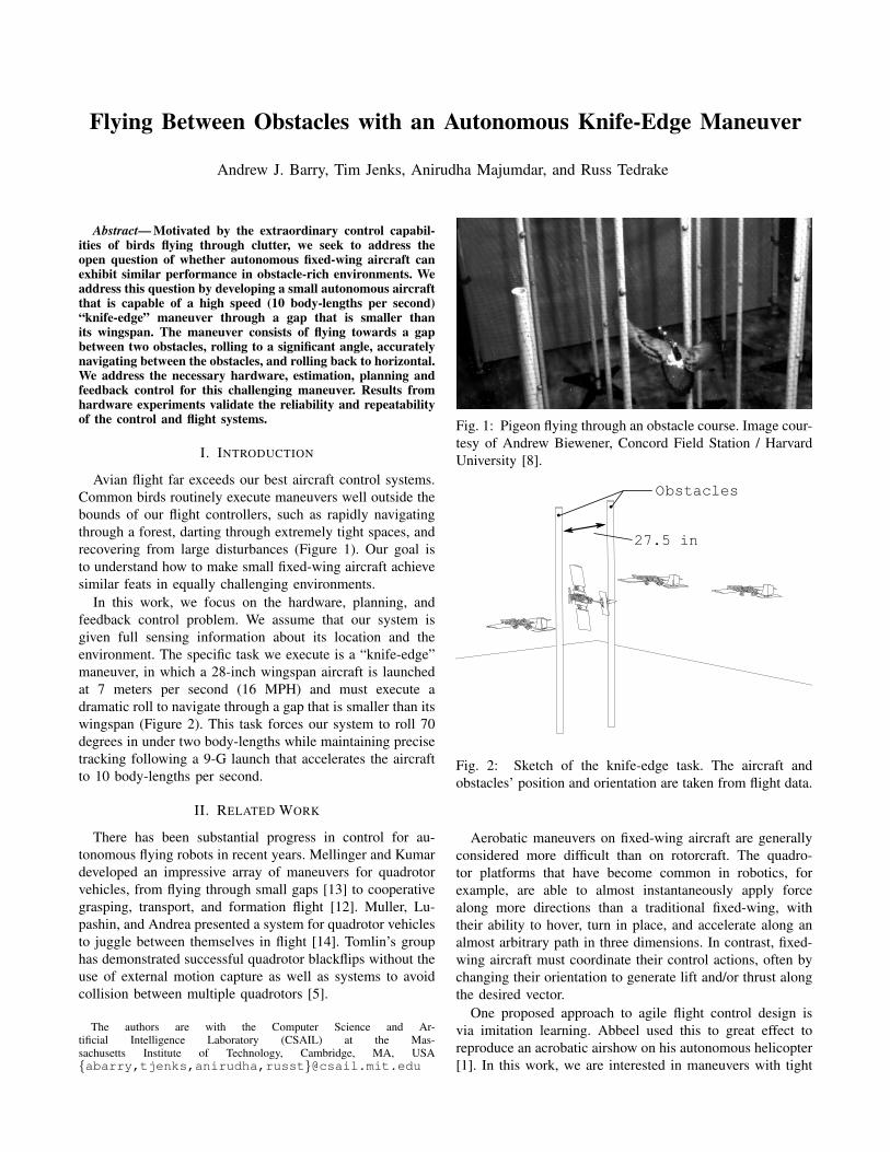
Avian flight far exceeds our best aircraft control systems.Common birds routinely execute maneuvers well outside thebounds of our flight controllers, such as rapidly navigatingthrough a forest, darting through extremely tight spaces, andrecovering from large disturbances (Figure 1). Our goal isto understand how to make small fixed-wing aircraft achievesimilar feats in equally challenging environments.

In this work, we focus on the hardware, planning, andfeedback control problem. We assume that our system isgiven full sensing information about its location and theenvironment. The specific task we execute is a “knife-edge”maneuver, in which a 28-inch wingspan aircraft is launchedat 7 meters per second (16 MPH) and must execute adramatic roll to navigate through a gap that is smaller than itswingspan (Figure 2). This task forces our system to roll 70degrees in under two body-lengths while maintaining precisetracking following a 9-G launch that accelerates the aircraftto 10 body-lengths per second.

II. RELATED WORK

There has been substantial progress in control for au-tonomous flying robots in recent years. Mellinger and Kumardeveloped an impressive array of maneuvers for quadrotorvehicles, from flying through small gaps [13] to cooperativegrasping, transport, and formation flight [12]. Muller, Lu-pashin, and Andrea presented a system for quadrotor vehiclesto juggle between themselves in flight [14]. Tomlin’s grouphas demonstrated successful quadrotor blackflips without theuse of external motion capture as well as systems to avoidcollision between multiple quadrotors [5].

The authors are with the Computer Science and Ar-tificial Intelligence Laboratory (CSAIL) at the Mas-sachusetts Institute of Technology, Cambridge, MA, USA{abarry,tjenks,anirudha,russt}@csail.mit.edu

Fig. 1: Pigeon flying through an obstacle course. Image cour-tesy of Andrew Biewener, Concord Field Station / HarvardUniversity [8].

Obstacles

27.5 in

Fig. 2: Sketch of the knife-edge task. The aircraft andobstacles’ position and orientation are taken from flight data.

Aerobatic maneuvers on fixed-wing aircraft are generallyconsidered more difficult than on rotorcraft. The quadro-tor platforms that have become common in robotics, forexample, are able to almost instantaneously apply forcealong more directions than a traditional fixed-wing, withtheir ability to hover, turn in place, and accelerate along analmost arbitrary path in three dimensions. In contrast, fixed-wing aircraft must coordinate their control actions, often bychanging their orientation to generate lift and/or thrust alongthe desired vector.

One proposed approach to agile flight control design isvia imitation learning. Abbeel used this to great effect toreproduce an acrobatic airshow on his autonomous helicopter[1]. In this work, we are interested in maneuvers with tight

Fig. 3: Experimental platform.

kinematic constraints: our aircraft must perform a perform a70-degree roll in 0.22 seconds immediately followed by a 60degree roll in the reverse direction in 0.16 seconds. Further-more, we are interested in algorithms that will allow planningthrough previously unknown obstacle fields. Although onecannot be sure, we felt that this class of maneuvers wouldbe difficult for even an extremely skilled pilot.

The work we present here builds more closely on theprevious work in fixed wing acrobatics. Cory used a similarapproach on a fixed-wing glider to perch on a wire [2].Sobolic’s system uses a similar aircraft model to transitionfrom the hover regime to forward flight [16].

One other key difference in the work we present hereis the use of a “wingeron” design that has not previouslybeen explored on agile autonomous aircraft. The design callsfor the use of entire wings as control surfaces and offersextremely high roll-rates at the cost of slightly more complexdynamics.

III. AIRCRAFT HARDWARE

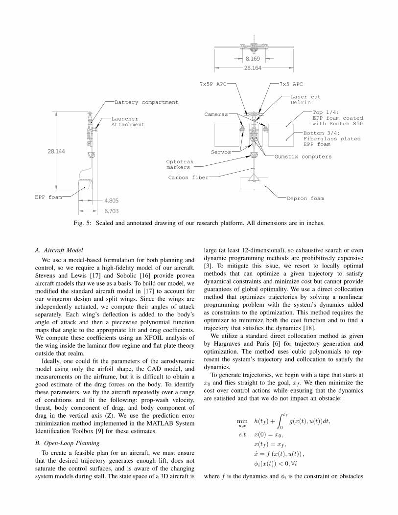
We have built an unmanned aerial vehicle (UAV) researchplatform to serve as the testbed for algorithms and as thefinal metric of performance (Figure 3). We use a “wingeron”design that does away with the traditional wing and aileronseen on most aircraft in favor of a wing that is completelyactuated; in other words, the entire wing rotates to act as acontrol surface. This greatly expands the aircraft’s roll ability,only saturating the roll rate when the wingeron approaches90o to the oncoming flow. The wingerons, however, compli-cate the flight dynamics due to the additional possibility of asingle wing stall during a turn. For example, if the aircraft isexecuting a right roll, the left wingeron will be deflected upto generate additional lift. Should that wingeron deflect toomuch, it will stall, causing a loss of lift and the possibilityof the aircraft rolling in the opposite direction.

We use an asymmetric wing optimized using XFOIL[4] for flight at 5-15 meters per second (Figure 4). Wecut the wing out of expanded polypropylene (EPP) foam,chosen for its ability to absorb kinetic impacts without

Fig. 4: Airfoil profile, designed to optimize lift at speeds of5-15 m/s.

permanent deformation. The wings are cut with a computer-controlled hot wire to produce the appropriate airfoil andthen strengthened with light-weave fiberglass on the trailingthree quarters to ensure that the wing does not significantlydeform when subjected to torsional stress.

For propulsion, we use small outrunner brushless DCmotors and APC propellers commonly found on aircraft ofthis scale. We use a two-motor, counter-rotating propellerdesign that reduces the torque on the airframe produced bychanging the throttle. For only a minor efficiency cost, weare able to effectively eliminate this effect, rendering the rolldynamics invariant to the time derivative of the throttle.

Our on-board electronics package is based around a ARMCortex-A8 running Linux connected to an Atmel micro-controller that is in turn connected to the motor speedcontrollers, actuator servo motors, 3 axis gyroscope, 3-axisaccelerometer, and 3-axis magnetometer.

Due to the limited space in our motion-capture environ-ment, we require a system to accelerate the plane to fullspeed very rapidly. We use stretched elastic to acceleratea carriage down an approximately meter-long (3.2 ft) rail,with a 9-G peak force. A bar in front of the aircraft holdsthe plane in place, even at full throttle, allowing us to releasethe aircraft while the motors are running. The carriage is tallenough to give clearance for the propellers.

IV. CONTROL

We denote the aircraft’s body-centric position in 3-dimensional space and characterize the aircraft dynamics,x = f(x, u), using a 12-dimensional state as follows:

x =[xp yp zp ψ θ φ U V W R Q P

]Txp, yp, and zp denote the aircraft position in the worldcoordinate frame. ψ, θ, and φ denote yaw, pitch, and rollrespectively. U , V , and W are the derivatives of the positionsexpressed in body-frame coordinates and R, Q, and Pare the aircraft angle derivatives expressed in body-framecoordinates.

We control five inputs on the aircraft: throttle and thedeflections of the elevator, rudder, left wingeron, and rightwingeron. We approximate these inputs as instantaneous toavoid adding additional states to our system.

u =

throttleelevatorrudder

wingeron leftwingeron right

Cameras

Gumstix computers

7x5 APC

Top 1/4:EPP foam coatedwith Scotch 850

Depron foam

7x5P APC

Optotrakmarkers

Carbon fiber

Laser cutDelrin

Bottom 3/4:Fiberglass platedEPP foam

Servos28.144

4.805

6.703

LauncherAttachment

EPP foam

Battery compartment

8.169

28.164

Fig. 5: Scaled and annotated drawing of our research platform. All dimensions are in inches.

A. Aircraft Model

We use a model-based formulation for both planning andcontrol, so we require a high-fidelity model of our aircraft.Stevens and Lewis [17] and Sobolic [16] provide provenaircraft models that we use as a basis. To build our model, wemodified the standard aircraft model in [17] to account forour wingeron design and split wings. Since the wings areindependently actuated, we compute their angles of attackseparately. Each wing’s deflection is added to the body’sangle of attack and then a piecewise polynomial functionmaps that angle to the appropriate lift and drag coefficients.We compute these coefficients using an XFOIL analysis ofthe wing inside the laminar flow regime and flat plate theoryoutside that realm.

Ideally, one could fit the parameters of the aerodynamicmodel using only the airfoil shape, the CAD model, andmeasurements on the airframe, but it is difficult to obtain agood estimate of the drag forces on the body. To identifythese parameters, we fly the aircraft repeatedly over a rangeof conditions and fit the following: prop-wash velocity,thrust, body component of drag, and body component ofdrag in the vertical axis (Z). We use the prediction errorminimization method implemented in the MATLAB SystemIdentification Toolbox [9] for these estimates.

B. Open-Loop Planning

To create a feasible plan for an aircraft, we must ensurethat the desired trajectory generates enough lift, does notsaturate the control surfaces, and is aware of the changingsystem models during stall. The state space of a 3D aircraft is

large (at least 12-dimensional), so exhaustive search or evendynamic programming methods are prohibitively expensive[3]. To mitigate this issue, we resort to locally optimalmethods that can optimize a given trajectory to satisfydynamical constraints and minimize cost but cannot provideguarantees of global optimality. We use a direct collocationmethod that optimizes trajectories by solving a nonlinearprogramming problem with the system’s dynamics addedas constraints to the optimization. This method requires theoptimizer to minimize both the cost function and to find atrajectory that satisfies the dynamics [18].

We utilize a standard direct collocation method as givenby Hargraves and Paris [6] for trajectory generation andoptimization. The method uses cubic polynomials to rep-resent the system’s trajectory and collocation to satisfy thedynamics.

To generate trajectories, we begin with a tape that starts atx0 and flies straight to the goal, xf . We then minimize thecost over control actions while ensuring that the dynamicsare satisfied and that we do not impact an obstacle:

minu,x

h(tf ) +

∫ tf

0

g(x(t), u(t))dt,

s.t. x(0) = x0,

x(tf ) = xf ,

x = f (x(t), u(t)) ,

φi(x(t)) < 0,∀i

where f is the dynamics and φi is the constraint on obstacles

as defined below.Our cost function focuses on the control actions of the

aircraft. The one-step cost is g = uTRu, where u is thecontrol vector introduced earlier. We let the system’s finalcost simply equal to the final time, promoting solutionsrequiring less time in the air: h = tf .

To ensure that our trajectory does not collide with ob-stacles, we add constraints based on the distance to eachobstacle. With the cost function and constraints, we simul-taneously balance avoiding obstacles and limiting controlactions. For the purposes of this trajectory, we use cylindricalobstacles that are infinitely tall and defined to be along theZ-axis.

We compute the distance from the vehicle to the obstacleby projecting both the aircraft and obstacle’s image onto theXY-plane. In this projection, we approximate the aircraft’sshape as a rectangle, taking the yaw, pitch, and roll anglesinto account. This projection results in our aircraft becoming“thinner” on the XY-plane as it rolls, promoting a high rollangle when maneuvering through the obstacles.

If we let d be the minimum distance from the projectedrectangle to the center of the obstacle’s projected circle, wecan use the following function for the constraint:

φi = tanh(r − d)

where r is the radius of the obstacle. Figure 6 visualizes theconstraint function at different roll angles.

C. Feedback Control with a Time-Varying Linear QuadraticRegulator

Inspired by the recent success with time-varying linearquadratic regulators (TVLQR) such as [1] and [2], we usethis method to perform feedback around our desired trajec-tory. In this formulation, we use a standard linear quadraticregulator (LQR) controller, but move the goal point at eachinstant in time, linearizing around the reference trajectory[15]. The algorithm is closely related to differential dynamicprogramming [11] with similar formulations for costs andresults for linear systems.

Given a nominal trajectory, x0(t), and a nominal controlinput, u0(t), we can define new coordinates centered aroundx0(t) as follows:

x(t) = x(t)− x0(t), u(t) = u(t)− u0(t)

Linearizing the time-varying dynamics of x(t), we obtain:

˙x(t) ≈ A(t)x(t) +B(t)u(t).

The control law is obtained by solving a Riccati differentialequation:

−S(t) = Q−S(t)B(t)R−1BTS(t)+S(t)A(t)+A(t)TS(t)

with final value conditions S(t) = Sf . Here, Q and R arepositive-definite cost-matrices. The feedback control law isthen given by:

u(x, t) = −R−1BT (t)S(t)x(t) = −K(t)x(t).

0

5

−505

−1

−0.5

0

0.5

Y (m)X (m)

(a) Roll set to 0o.

0

5

−505

−1

−0.5

0

0.5

Y (m)X (m)

(b) Roll set to 70o.

Fig. 6: Constraint functions for two obstacles and differentroll configurations as a 2D slice of space (all states otherthan x, y, and φ are set to zero). Obstacles are shown asblue cylinders. The optimization is constrained to allow theaircraft only to pass through locations where the values areless than zero. A tanh() function is used to give the optimizera gradient that is easy to follow.

The TVLQR controller requires some hand-tuningof the cost matrix before it will track the open-loop trajectory adequately. We performed this hand-tuning based on repeated flights and comparisonsbetween the system’s actual and desired paths. Thecosts used in the knife-edge task are as follows: Q =diag([100, 100, 100, 1000, 100, 100, 10, 10, 10, 42, 10, 10]),R = diag([0.2, 2, 2, 0.6, 0.6]).

D. State Estimator

Our motion capture system reports the pose of the planeat 70 Hz. We use finite differences combined with a Lu-enberger observer [10] to obtain estimates of the derivativesof the positions and angles expressed in the body frame.Denoting our dynamics model by x = f(x, u), we can writethe dynamics of the estimated state, x, as:

˙x = f(x, u) + L(y − x)

where, y denotes the observation and L is the hand-tunedLuenberger gain. y consists of pose estimates reported by the

27.5

108.3

Vertical obstacles

Fig. 7: Diagram of the experimental setup (to scale). Alldimensions are in inches.

motion capture system and derivatives estimated from finitedifferencing. At each time-step, an Euler update is used toobtain the current estimated state:

x[t] = x[t− dt] + ˙x[t]dt.

Since the pose estimates reported by the motion capturesystem are reliable, we ignore the pose variables in theestimated state and keep only the derivative variables. Duringthe short periods of time when the motion capture markersare occluded by obstacles, we estimate the state by forwardsimulating the aircraft model.

V. RESULTS

Our experiment consists of two poles 0.7 meters (27.5inches) apart and 2.75 meters (9 feet) in front of ourlaunching system. Figure 7 gives an scaled drawing of thesetup.

The hardware system has proven to have impressive per-formance and to be robust to multiple failures. We haveflown hundreds of test flights, each ending with an impactinto a net, with only minor, repairable hardware failures.The airframe is robust to conditions created from sensing,control, and computational failure, as well as loss of powerand unintended impact with the launching system. None ofthese minor repairs required changing model parameters.

We note that the launching mechanism produced consis-tent initial conditions, simplifying the modeling and tuningproblems. This allowed us to rely on the launcher to place theaircraft in flight in states near where the open-loop trajectorystarted.

We find that the system’s tracking is sufficient for repeatedflights through the obstacle field without collision. We haveflown 9 flights through the vertical obstacles using twodifferent locally optimal trajectories. On every flight theaircraft successfully navigated the gap without collision.

Figure 8 shows the results of six repeated flights with thissystem, the desired trajectory, and the result of running thesystem without feedback. Figure 10 gives snapshots of theaircraft performing this trajectory in our test environment.

It is interesting to note that the feedback system primarilycorrects for errors in the models. Figure 9 shows action-tapesfor six closed-loop executions and the open-loop referencefor the control surfaces. The closed-loop tapes are consistent,but they differ from the open-loop tape, indicating that thefeedback system is working to correct errors in modeling.

0 1 2 3 4 5

−20

0

20

40

60

80

100

120

X (m)

Roll

(deg)

Reference

Open Loop

Closed Loop

(a) Aircraft flight data for roll vs. forward flight. Red shows flightswith the closed-loop controller running and black shows flightsrunning only the open-loop tape.

−1 0 1 2 3 4 5

−1.5

−1

−0.5

0

0.5

1

1.5

X (m)

Z (

m)

Reference

Open Loop

Closed Loop

(b) Comparison of forward flight (X-axis) vs. height (Z-axis). Notethat the Z axis is plotted in reverse to give a more intuitive view ofthe aircraft’s height (in our coordinate system increasing Z movestowards the ground).

Fig. 8: Motion capture data from the aircraft in flightcompared with the planned knife-edge maneuver. We showboth open-loop (black) and closed-loop (red) flights. Thegaps in the data occur when the plane’s markers pass by theobstacles, causing the motion capture system to lose sight ofthe plane for a small period of time.

A. Extension to Horizontal Obstacles

The knife-edge maneuver demonstrates good tracking andsystem performance but does not require the system toperform more than one maneuver during a flight. The samesystem should be able to perform multiple maneuvers. Totest this, we added two horizontal obstacles after the twovertical obstacles. This configuration requires the aircraft toquickly roll back to level flight and maintain altitude trackingto succeed in avoiding both obstacles.

We used our existing model to plan a new trajectory withhorizontal obstacles, adding constraints similar to those usedfor the vertical barriers. We then tuned the LQR costs for thattrajectory to improve tracking. Figure 12 shows snapshotsof the flight and Figure 13 show images from the on-board

−0.2 0 0.2 0.4 0.6

−50

0

50

Time (s)

Co

mm

an

de

d D

efle

ctio

n (

de

g)

(a) Left wingeron

−0.2 0 0.2 0.4 0.6

−50

0

50

Time (s)

Co

mm

an

de

d D

efle

ctio

n (

de

g)

(b) Right wingeron

−0.2 0 0.2 0.4 0.6

−50

0

50

Time (s)

Co

mm

an

de

d D

efle

ctio

n (

de

g)

(c) Elevator

−0.2 0 0.2 0.4 0.6

−50

0

50

Time (s)

Co

mm

an

de

d D

efle

ctio

n (

de

g)

(d) Rudder

Fig. 9: Comparison between open-loop control tapes (blue)and closed-loop tapes (red) for the knife-edge trajectory.Note the similarity between six successful runs of the knife-edge trajectory and the dissimilarity between those and theopen-loop tape. This indicates that our feedback system isprimarily correcting for model inaccuracies.

camera during flight.

VI. FUTURE WORK AND CONCLUSION

A. FPGA Vision and Outdoor Navigation

Recent work on FPGA vision systems has provided en-couraging results that our platform may be able to collect andprocess information about its surroundings at 120 frames persecond [7]. We are considering moving our platform out ofa motion capture environment, adding an FPGA processor,and determining where obstacles are in real time.

Moving out of a motion capture environment will requirea substantial sensing and estimation effort, which will extendour sensors to airspeed, barometric altitude, GPS, and others.Our aircraft is capable of carrying these sensors and we lookforward to UAVs that can fly at high speed, identifying andavoiding obstacles faster than any human pilot.

B. Conclusion

We have demonstrated a system that is capable of per-forming a knife-edge maneuver, rolling 70 degrees in undertwo body-lengths, while moving at over 10 body-lengths persecond. Our system, using an aerodynamic model, directcollocation based trajectory optimization, and TVLQR iscapable of performing the maneuver robustly. Finally, weextend the work to a more challenging obstacle field andshow that the techniques are sufficient for that task as well.

Fig. 10: Sequence of stills from a knife-edge maneuver. Eachimage is 0.0417 seconds (41.7ms) after the previous. Theentire set captures a total of 0.292 seconds. The full flight,including onboard video, is shown in the video attachment.

Fig. 11: Sequence of stills from an onboard camera duringthe knife-edge maneuver. Each image is 0.083 seconds(83ms) after the previous. The entire set captures a total of0.583 seconds.

Fig. 12: Sequence of stills from a four-obstacle maneuver.As before, each image is 0.0417 seconds (41.7ms) after theprevious. The entire set captures a total of 0.292 seconds.

Fig. 13: Sequence of stills from an onboard camera duringthe four-obstacle knife-edge maneuver. Each image is 0.083seconds (83ms) after the previous. The entire set captures atotal of 0.583 seconds.

VII. ACKNOWLEDGEMENTS

This work was supported by ONR MURI grant N00014-09-1-1051. Andrew Barry is partially supported by a Na-tional Science Foundation Graduate Research Fellowship.Anirudha Majumdar is partially supported by the SiebelScholars Foundation.

REFERENCES

[1] P. Abbeel, A. Coates, M. Quigley, and A. Y. Ng. An application ofreinforcement learning to aerobatic helicopter flight. In Proceedingsof the Neural Information Processing Systems (NIPS ’07), volume 19,December 2006.

[2] R. Cory. Supermaneuverable Perching. PhD thesis, MassachusettsInstitute of Technology, June 2010.

[3] M. Diehl, H. Bock, H. Diedam, and P. Wieber. Fast direct multipleshooting algorithms for optimal robot control. Fast Motions inBiomechanics and Robotics, pages 65–93, 2006.

[4] M. Drela and H. Youngren. Xfoil 6.94 user guide. 2001.[5] J. H. Gillula, G. M. Hoffmann, H. Huang, M. P. Vitus, and C. Tomlin.

Applications of hybrid reachability analysis to robotic aerial vehicles.The International Journal of Robotics Research, 2011.

[6] C. R. Hargraves and S. W. Paris. Direct trajectory optimization usingnonlinear programming and collocation. J Guidance, 10(4):338–342,July-August 1987.

[7] D. Honegger, P. Greisen, L. Meier, P. Tanskanen, and M. Pollefeys.Real-time velocity estimation based on optical flow and disparitymatching. To appear, Intelligent Robots and Systems (IROS) 2012,Oct. 2012.

[8] H. Lin, I. Ros, and A. Biewener. Through the eyes of a bird: A vision-based model for pigeon obstacle avoidance flights. In preparation.

[9] L. Ljung. System identification toolbox for use with matlab. 2007.[10] D. Luenberger. An introduction to observers. Automatic Control, IEEE

Transactions on, 16(6):596–602, 1971.[11] B. Mayne. A second-order gradient method for determining optimal

trajectories of non-linear discrete-time systems. International Journalof Control, 3(1):85–95, 1966.

[12] Mellinger, D., Shomin, M., Michael, N., Kumar, and V. Cooperativegrasping and transport using multiple quadrotors. In Proceedings of theinternational symposium on distributed autonomous robotic systems,2010.

[13] D. Mellinger, N. Michael, and V. Kumar. Trajectory generationand control for precise aggressive maneuvers with quadrotors. InProceedings of the 12th International Symposium on ExperimentalRobotics (ISER 2010), 2010.

[14] M. Muller, S. Lupashin, and R. D’Andrea. Quadrocopter ball juggling.In Intelligent Robots and Systems (IROS), 2011 IEEE/RSJ Interna-tional Conference on, pages 5113–5120. IEEE, 2011.

[15] P. Reist and R. Tedrake. Simulation-based LQR-trees with input andstate constraints. In Proceedings of the International Conference onRobotics and Automation (ICRA), 2010.

[16] F. M. Sobolic. Agile flight control techniques for a fixed-wing aircraft.Master’s thesis, Massachusetts Institute of Technology, June 2009.

[17] B. Stevens and F. Lewis. Aircraft Control and Simulation. John Wiley& Sons, Inc., 1992.

[18] O. von Stryk. Numerical solution of optimal control problems by directcollocation. In Optimal Control, (International Series in NumericalMathematics 111), pages 129–143, 1993.