1

Exploring the use of LIDAR data from Autonomous Cars for Estimating Traffic Flow Parameters and Vehicle Trajectories

Date:October2017

MecitCetin,PhD,AssociateProfessor,OldDominionUniversityCemSazara,PhDstudent,OldDominionUniversityRezaVataniNezafat,PhDstudent,OldDominionUniversity

Preparedby:TransportationResearchInstitute(TRI)OldDominionUniversity135KaufmanHallNorfolk,VA23529Preparedfor:Mid-AtlanticTransportationSustainabilityUniversityTransportationCenter

FINAL REPORT

2

UniversityofVirginiaCharlottesville,VA22904

1. Report No.

2. Government Accession No. 3. Recipient’s Catalog No.

4. Title and Subtitle Exploring the use of LIDAR data from Autonomous Cars for Estimating Traffic Flow Parameters and Vehicle Trajectories

5. Report Date 10/09/2017

6. Performing Organization Code

7. Author(s) Mecit Cetin, Cem Sazara, Reza Vatani Nezafat

8. Performing Organization Report No.

9. Performing Organization Name and Address Old Dominion University, Norfolk, VA 23529

10. Work Unit No. (TRAIS

11. Contract or Grant No. DTRT13-G-UTC33

12. Sponsoring Agency Name and Address US Department of Transportation Office of the Secretary-Research UTC Program, RDT-30 1200 New Jersey Ave., SE Washington, DC 20590

13. Type of Report and Period Covered Final 11/5/15 – 9/30/17

14. Sponsoring Agency Code

15. Supplementary Notes

16. Abstract

LIDAR has become one of the major enabling technologies for autonomous vehicles. LIDAR sensors generate 3D point cloud data around the instrumented vehicle. These data enable detailed localization of both fixed and moving objects in the surrounding environment. In this project, various aspects of LIDAR data processing are studied with an emphasis on exploiting such data for estimating traffic flow parameters. To achieve that, LIDAR data are collected in the field by an instrumented vehicle under different traffic conditions. Data processing and machine learning algorithms are developed to detect and classify vehicles based on the point cloud data. These algorithms help track ambient vehicles and extract their trajectories. From the extracted trajectories, both microscopic and macroscopic traffic flow parameters can then be estimated. In the case when some vehicle trajectories are partially observed or missing for a short duration, e.g., due to occlusion, this report shows how such trajectories could be completed by employing car following models. To demonstrate the use of trajectory data for estimating traffic flow parameters, a richer dataset with all vehicle trajectories, i.e., the NGSIM data, are utilized. Models are developed to predict traffic density, or the number of unobserved vehicles between two known trajectories, under congested conditions from a sample of trajectories. Under the dense traffic conditions analyzed, the results show that the number of unobserved vehicles between two probes can be predicted with an accuracy of ±1 vehicle almost always.

17. Key Words LIDAR, 3D point cloud, Kalman Filter, microscopic traffic flow, macroscopic traffic flow

18. Distribution Statement No restrictions. This document is available from the National Technical Information Service, Springfield, VA 22161

3

19. Security Classif. (of this report) Unclassified

20. Security Classif. (of this page) Unclassified

21. No. of Pages 28

22. Price

4

Acknowledgements

TheauthorswouldliketothankMid-AtlanticTransportationSustainabilityCenter–Region3UniversityTransportationCenter(MATSUTC)forfundingthisproject.

Disclaimer

The contentsof this report reflect the viewsof theauthors,whoare responsible for the factsand theaccuracyoftheinformationpresentedherein.ThisdocumentisdisseminatedunderthesponsorshipoftheU.S. Department of Transportation’s University Transportation Centers Program, in the interest ofinformationexchange.TheU.S.Governmentassumesnoliabilityforthecontentsorusethereof.

5

TableofContents1. Problem:...............................................................................................................................................6

2. ApproachandResearchObjectives:.....................................................................................................6

3. Introduction:........................................................................................................................................6

4. Methodology:.......................................................................................................................................8

DataCollectionandProcessing:...............................................................................................................8

DataAnalysis:...........................................................................................................................................9

5. ResearchFindings:................................................................................................................................9

DataCollection:........................................................................................................................................9

VehicleClassification:.............................................................................................................................10

GroundDetection:..................................................................................................................................10

TargetDetectionandClassification:.......................................................................................................12

TargetTracking:......................................................................................................................................13

MicroscopicandMacroscopicTrafficParameters.................................................................................17

ConstructingVehicleTrajectories:.........................................................................................................17

Estimatingtrafficdensityfromtrajectories:..........................................................................................22

6. Conclusions:.......................................................................................................................................28

7. References:.........................................................................................................................................28

6

1. Problem:Traditionally, fixed-point detectors such as loop detectors have been the dominant technology forcollectingtrafficflowdata.Fixedpointsensors,bydefinition,onlycollectdataatthespecific locationstheyareinstalled.Ontheotherhand,vehicletrackingandlocalizationtechnologies,suchasGPS,enablemeasuringtrafficflowcharacteristicsalongthepathsofsocalledprobevehicles.Obviously,trackingaGPS-equippedmobileconsumerdevice(s)withinthevehiclealsoenablesgeneratingsimilardata.Datafromthesesourceshavebeenusedinstudyingtrafficflowphenomena[1-3].Mobilesensorsprovidemorediverseinformationcomparedtofixedlocationdetectorsastheyarenotlimitedtocertaindatacollectionlocations.Withtheemergenceofautonomousvehicles,itisnowpossibletoexpectanothersourcedatathatwouldbecomecommonlyavailableastheseentertheconsumermarket.AutonomousvehiclesaretypicallyequippedwithLIDARorothersimilarsensorstodetectandtrackobstaclesinthesurroundingenvironment.LIDARalsoprovidesameanstodetectandtrackothervehiclesaroundtheautonomouscar.Thereisverylimitedresearchonhowdatafromsuchvehiclescouldbeutilizedtoestimatetrafficflowparameters.Inthisproject,3DpointcloudsdatafromaLIDARinstalledonavehicleareusedforextractinginformationrelevantformodelingtrafficflow.Suchdataareveryrichandhavetheadvantageofdefiningtheenvironmentinmoredetailbutalsorequirefastprocessingmethodsduetolargesizeofthedata.Thisreport discusses LDIAR data collection and processing to estimate micro and macro traffic flowparameters.

2. ApproachandResearchObjectives:ThemaingoalofthisstudyistoestimatetrafficflowparameterswiththehelpofLIDAR.Thespecificgoalsandtheapproachoftheproposedresearchare:

1. CollectsampleLIDARdataunderdifferenttrafficconditionsonfreewaysandurbanarterials inHamptonRoads

2. DevelopalgorithmstodetectvehiclesaroundaLIDAR-equippedcarandclassifythembasedonvehiclesize.

3. DevelopalgorithmstotrackothervehicleswhilewithintheLIDARrange4. Estimatemacroscopictrafficflowparametersbasedonthedetectedvehiclesalongthepathof

theLIDAR-equippedvehicle

3. Introduction:Environmentdetectionisoneofthekeyaspectofautonomousdrivingtechnologies.Detectingobstaclesaroundtheautonomousvehicle,suchasmovingorparkedcars,pedestrians,trees,curbsetc.,accuratelyand reliably is a challenge. To accomplish that, autonomous driving systems use sensor and camerasystemstosuccessfullynavigatewhileavoidingobstacles.LIDARshavebecomeanimportantpartofthesedrivingsystems.LIDARisaremotesensingtechnologythatmeasuresdistancetoatargetbysendinglaserbeamsandmeasuringreturnedbeams.LIDARsproviderichspatial informationabouttheenvironmentsurroundingthesensor.Inthisproject,3DVelodyneVLP-16LIDARsensorisused[4].Thissensorhas16laserbeamswithdifferentpitchangles,in2degreesincrement,ona360-degreerotatingunit.Figure1.belowillustratesaVLP-16sensorandtheorientationofthe16laserbeams(seealsoTable1).

7

Figure1.LIDARandlaserstructure

The unit allows observing 360-degree horizontal and 30-degree vertical field of view producingapproximately30,000pointsinasinglescan.Itcandetecttargetsupto100mawaywithinacirclefieldofdetection.Itsrotationfrequencycanbeadjustedbetween5to20Hz.Inthisproject,itisusedat10Hzwhichmeans a snapshot of the environment is taken in every 0.1 seconds. In this project, data arecollectedonurbanroadswithaVelodyneVLP-16sensor.

Table1.LIDARlaserverticalanglesLaserID Verticalangle0 -15

1 12 -133 -34 -11

5 56 -97 78 -7

9 910 -511 1112 -3

13 1314 -115 15

Anillustrationofthe3DLIDARdataisinFigure2.Itprovidesdetailedinformationaboutsurroundingofthevehicle.Differentcolorsdesignatedifferent intensity levelswhich increasewithreflectivesurfacessuchasmetals.

8

Figure2.LIDARdatapointsnearanintersection

4. Methodology:Themethodologyinthisprojectcanbedividedintotwomajorparts:(i)DataCollectionandProcessingand(ii)DataAnalysis.Thesearediscussednext.

Data Collection and Processing: Datacollectionpartisaccomplishedbymountingthe3DLIDARonasedanvehicleandmakingmultipletripsunderdifferenttrafficconditions.

Figure3.Dataprocessingsteps

ThedataprocessingstepstartswitheachnewLIDARscanandrepeatsforeverynewLIDARscan.EveryLIDARscan,whichisalsocalledaframe,isrecordedwith10Hzfrequency.Thisgives10LIDARframesforeverysecond.LIDARpointsgothroughthe“Classification”sectionwherevehiclesaredetected.Then,thisdetectedvehicleinformationissenttothe“Tracking&Dataassociation”sectionwheremeasurementsarerelatedtothepreviousmeasurementsandtracking(relatingtothepreviousmeasurements)isdone.In this part, Kalman Filtering is used to track targets and data association is done with HungarianAlgorithm.Output of the “Tracking&Data association” step produces vehicle trajectory information.

9

Trajectorydatacollectioniscrucialasitpreparesthebasisdataforthemicro&macrotrafficanalysispartoftheproject.

Data Analysis: Inthispart,weusethedatacollectedinthepreviousstepandinvestigatemicro-macrotrafficparameters.Makingtripsondifferenttypesofroadsunderdifferentconditionshelpedusgettingadiversedatasetthatprovideswiderangeoftrafficsituationssuchasstop-go,heavyandfree-flowtraffic.Dataanalysispart is divided into two sections: “Microscopic” Traffic Study and “Macroscopic” Traffic Study. In“Microscopic” part, we studied microscopic traffic phenomena which mostly includes car-followingmodels.Collecteddataisusedtocalibratedifferentcarfollowingmodels:Gipps,IDM,NewellandPipe’s.Thesemodelsprovideinformationaboutdrivingbehavior.In“Macroscopic”studypart,NGSIMdatasetisused to createamodel forestimatingnumberof vehiclesbetweenprobevehiclesunder stop-and-goconditions. Unsupervised and supervisedmethods are developed and used to estimate the unknownnumberofvehiclesbetweenprobesandthenit isusedtocalculatethemacroscopictrafficparametertrafficdensity.Asafuturework,thisworkwillbeextendedtoincludeLIDARdatainadditiontotheNGSIMdataintheestimationmethods.

5. ResearchFindings:Inthissection,weexplaindevelopedalgorithmsandmethodstoaddressourresearchobjectives.

Data Collection: Our3DVelodyneLIDARismountedontheroofofourvehicleand3DLIDARdataiscollected.WedroveLIDARequippedvehiclesindifferenttrafficconditionsonurbanroadsandhighwaysinHamptonRoadsRegioninVirginia.BelowinFigure4,ourdatacollectionvehiclecanbeseen.

Figure4.OurvehiclewithLIDARismarkedwithredcircle

10

HamptonRoadsareaprovidesrichtrafficinformationasitincludesvarioustypesofinfrastructuressuchasbridgesandtunnels.LIDARdataiscollectedwithmultipletripsondifferentroutestocapturediversedrivingconditions.TheseroutesaremarkedwithblueinFigure5.

Figure5.Datacollectionroutes

Vehicle Classification: Vehicleclassificationconsistsoftwoparts:Grounddetectionandtargetclassification.Grounddetectionand target detection are closely related. Data coming from 3D LIDAR is first processed for grounddetectionandthenfortargetorobstacledetectionandclassification.Ingrounddetection,groundpointsaredetectedandremovedfromthecompletesetofpoints.Thentargetdetection-classificationisappliedontheremainingpoints.

Ground Detection: Oneof thechallengesdealingwithLIDARdata isdistinguishinggroundpoints fromotherpoints.Datacomingfrom3DLIDARisfirstprocessedforgrounddetection.Manymethodsintheliteratureassumesaflatgroundsurfaceandsimplyappliesaheightthreshold[5-7].Thiscausesproblemsinsomedifferentsituationswheretheroadisnotflat.WeshowanexampleofthatsituationfromourLIDARdatainFigure6.AsshowninFigure6(right),roadsandtheircrosssectionsarenotcompletelyflat,andtheymaybecurved.In[8,9],groundpointsarecalculatedbyfittingaplaneusingRANSACalgorithm.Thismethodhastheassumptionthatgroundneedstobeplanarandhaslimitationsiftheroadhascurvesorslopeononeside.In[10],authorsproposedagrid(cell)basedmethodwheregroundisdetectedusingaverageandvariance of heights falling into each cell.We applied an approach similar to themethod in [10] anddevelopedasimplerule-basedmethodtoidentifygroundpointsaccurately.Advantageofourmethodis

11

thatweinvestigateeachpointinagridcellseparatelybecauseeachcellmaycontainbothgroundandnon-groundpoints.

Figure6.Lidarscanprojectedinto2Dspace.Ontheleftprojectiontox,yaxisandrighttox,zaxis.

Wedefinedaregionofinterestof40meterslongand13meterswideandvehicledetection-classificationisdoneinthisfield.3DLIDARscanisprojectedontox-yspaceanddiscretizedinto0.25x0.25metersgridcellswhichcreatesagridwith52x160cells.Minimumheightineachcellwasfound,andanypointwithaheightlessthantheminimumheightinthecellplusaconstant(α)isconsideredtobelongtotheground.This condition is only appliedwhere theminimum height in the cell is less than a constant (β). Thisprocedureisappliedoneachcell.TheresultofthismethodonthesameLIDARscaninFigure6isgivenbelowinFigure7.Theredcolorsshowthedetectedground.

Figure7.Asampleresultofgrounddetection

Thisgrounddetectionalgorithmcanbeexpressedas:

𝑝" = 𝑔𝑟𝑜𝑢𝑛𝑑,ℎ𝑒𝑖𝑔ℎ𝑡 𝑝" < min ℎ𝑒𝑖𝑔ℎ𝑡 𝑐𝑒𝑙𝑙 𝑖, 𝑗 + 𝛼 𝑎𝑛𝑑min ℎ𝑒𝑖𝑔ℎ𝑡 𝑐𝑒𝑙𝑙 𝑖, 𝑗 < 𝛽𝑛𝑜𝑛 − 𝑔𝑟𝑜𝑢𝑛𝑑, 𝑒𝑙𝑠𝑒

(1)

12

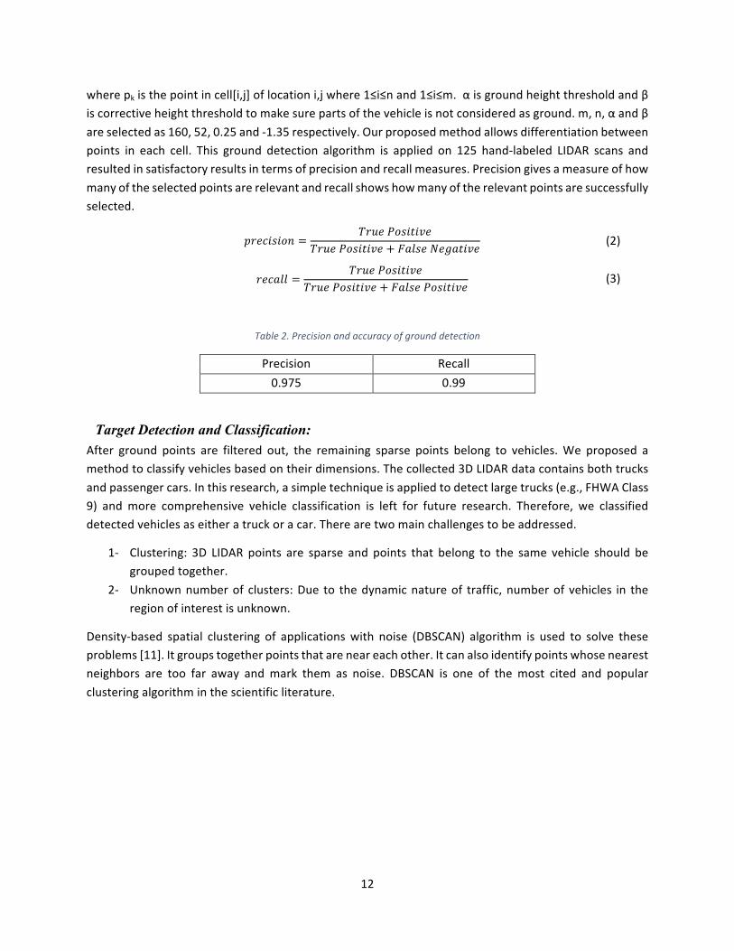
wherepkisthepointincell[i,j]oflocationi,jwhere1≤i≤nand1≤i≤m.αisgroundheightthresholdandβiscorrectiveheightthresholdtomakesurepartsofthevehicleisnotconsideredasground.m,n,αandβareselectedas160,52,0.25and-1.35respectively.Ourproposedmethodallowsdifferentiationbetweenpoints in each cell. This ground detection algorithm is applied on 125 hand-labeled LIDAR scans andresultedinsatisfactoryresultsintermsofprecisionandrecallmeasures.Precisiongivesameasureofhowmanyoftheselectedpointsarerelevantandrecallshowshowmanyoftherelevantpointsaresuccessfullyselected.

𝑝𝑟𝑒𝑐𝑖𝑠𝑖𝑜𝑛 =𝑇𝑟𝑢𝑒𝑃𝑜𝑠𝑖𝑡𝑖𝑣𝑒

𝑇𝑟𝑢𝑒𝑃𝑜𝑠𝑖𝑡𝑖𝑣𝑒 + 𝐹𝑎𝑙𝑠𝑒𝑁𝑒𝑔𝑎𝑡𝑖𝑣𝑒 (2)

𝑟𝑒𝑐𝑎𝑙𝑙 =𝑇𝑟𝑢𝑒𝑃𝑜𝑠𝑖𝑡𝑖𝑣𝑒

𝑇𝑟𝑢𝑒𝑃𝑜𝑠𝑖𝑡𝑖𝑣𝑒 + 𝐹𝑎𝑙𝑠𝑒𝑃𝑜𝑠𝑖𝑡𝑖𝑣𝑒 (3)

Table2.Precisionandaccuracyofgrounddetection

Precision Recall0.975 0.99

Target Detection and Classification: After ground points are filtered out, the remaining sparse points belong to vehicles.We proposed amethodtoclassifyvehiclesbasedontheirdimensions.Thecollected3DLIDARdatacontainsbothtrucksandpassengercars.Inthisresearch,asimpletechniqueisappliedtodetectlargetrucks(e.g.,FHWAClass9) andmore comprehensive vehicle classification is left for future research. Therefore, we classifieddetectedvehiclesaseitheratruckoracar.Therearetwomainchallengestobeaddressed.

1- Clustering: 3D LIDAR points are sparse and points that belong to the same vehicle should begroupedtogether.

2- Unknownnumberof clusters:Due to thedynamicnatureof traffic, numberofvehicles in theregionofinterestisunknown.

Density-based spatial clustering of applicationswith noise (DBSCAN) algorithm is used to solve theseproblems[11].Itgroupstogetherpointsthatareneareachother.Itcanalsoidentifypointswhosenearestneighbors are too far away andmark them as noise. DBSCAN is one of themost cited and popularclusteringalgorithminthescientificliterature.

13

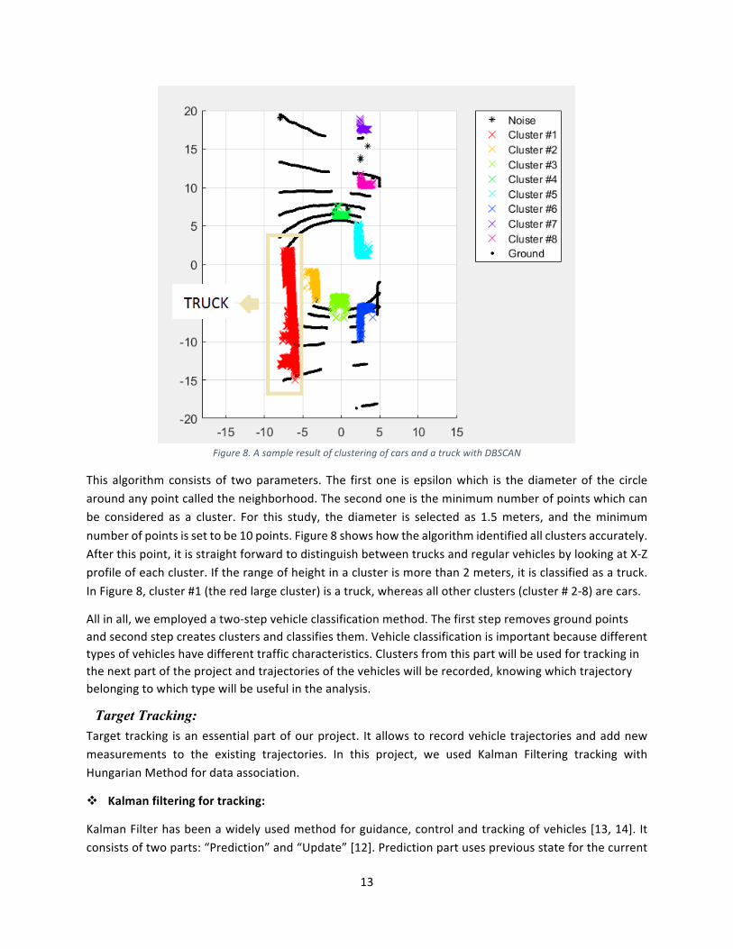
Figure8.AsampleresultofclusteringofcarsandatruckwithDBSCAN

This algorithmconsistsof twoparameters. The firstone is epsilonwhich is thediameterof the circlearoundanypointcalledtheneighborhood.Thesecondoneistheminimumnumberofpointswhichcanbe considered as a cluster. For this study, the diameter is selected as 1.5meters, and theminimumnumberofpointsissettobe10points.Figure8showshowthealgorithmidentifiedallclustersaccurately.Afterthispoint,itisstraightforwardtodistinguishbetweentrucksandregularvehiclesbylookingatX-Zprofileofeachcluster.Iftherangeofheightinaclusterismorethan2meters,itisclassifiedasatruck.InFigure8,cluster#1(theredlargecluster)isatruck,whereasallotherclusters(cluster#2-8)arecars.

Allinall,weemployedatwo-stepvehicleclassificationmethod.Thefirststepremovesgroundpointsandsecondstepcreatesclustersandclassifiesthem.Vehicleclassificationisimportantbecausedifferenttypesofvehicleshavedifferenttrafficcharacteristics.Clustersfromthispartwillbeusedfortrackinginthenextpartoftheprojectandtrajectoriesofthevehicleswillberecorded,knowingwhichtrajectorybelongingtowhichtypewillbeusefulintheanalysis.

Target Tracking: Targettracking isanessentialpartofourproject. Itallowstorecordvehicletrajectoriesandaddnewmeasurements to the existing trajectories. In this project, we used Kalman Filtering tracking withHungarianMethodfordataassociation.

v Kalmanfilteringfortracking:

KalmanFilterhasbeenawidelyusedmethodforguidance,controlandtrackingofvehicles[13,14].Itconsistsoftwoparts:“Prediction”and“Update”[12].Predictionpartusespreviousstateforthecurrent

14

stateprediction.Itdoesn’tincludeanyobservationinformation,soitiscalled“apriory”estimate.Intheupdatepart,currentestimateisupdatedusingthecurrentobservation,therefore,itiscalled“aposteriori”estimate.

State“s”attime“k”calculatedbymultiplyingstatetransitionmodel“F”attime“k”bystate“s”attime“k-1”andaddingprocessnoise“w”attime“k”.

1k k k ks F s w-= + (4)

whereprocessnoisewkisdrawnfromN(0,Qk)withzeromeanandcovarianceQk

Observation“z”attime“k”iscalculatedbymultiplyingstate“s”attime“k”byobservationmodel“H”attime“k”andaddingobservationnoise“v”attime“k”.

k k k kz H s v= + (5)

whereobservationnoisevkisdrawnfromN(0,Rk)withzeromeanandcovarianceRk

“Prediction”step:

Systemstateispredictedby

/ 1 1/ 1ˆ ˆk k k k ks F s- - -= (6)

Errorcovariancematrixispredictedby

/ 1 1/ 1T

k k k k k k kP F P F Q- - -= + (7)

where“P”denotescovariancematrixwhichyieldshowaccuratethestateestimationis.

“Update”step:

Measurementinnovationresidual:

/ 1ˆk k k k ky z H s -= -! (8)

Innovationcovariance:

/ 1T

k k k k k kC R H P H-= + (9)

OptimalKalmangain:

1/ 1

Tk k k k kK P H C -

-= (10)

Updatedstateestimate:

/ / 1ˆ ˆk k k k k kx x K y-= + ! (11)

Updatedestimatecovariance:

15

/ / 1( )k k k k k kP I K H P -= - (12)

In applying this filter toourproblemofobject tracking,weusedataprojectedontoa2D-space (x,y).Therefore,statesisgivenby[x,y]Twherexisxcoordinate,yisycoordinate.Observationzisthetrackedobject’smeasuredlocationgivenby[x,y]T

v Multi-targettrackingwithHungarianmethod:

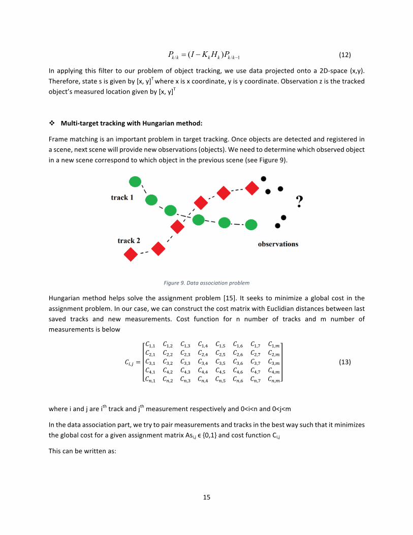
Framematchingisanimportantproblemintargettracking.Onceobjectsaredetectedandregisteredinascene,nextscenewillprovidenewobservations(objects).Weneedtodeterminewhichobservedobjectinanewscenecorrespondtowhichobjectinthepreviousscene(seeFigure9).

Figure9.Dataassociationproblem

Hungarianmethodhelps solve theassignmentproblem [15]. It seeks tominimizea global cost in theassignmentproblem.Inourcase,wecanconstructthecostmatrixwithEuclidiandistancesbetweenlastsaved tracks and new measurements. Cost function for n number of tracks and m number ofmeasurementsisbelow

𝐶C,D =

𝐶E,E 𝐶E,F 𝐶E,G 𝐶E,H 𝐶E,I 𝐶E,J 𝐶E,K 𝐶E,L𝐶F,E 𝐶F,F 𝐶F,G 𝐶F,H 𝐶F,I 𝐶F,J 𝐶F,K 𝐶F,L𝐶G,E 𝐶G,F 𝐶G,G 𝐶G,H 𝐶G,I 𝐶G,J 𝐶G,K 𝐶G,L𝐶H,E 𝐶H,F 𝐶H,G 𝐶H,H 𝐶H,I 𝐶H,J 𝐶H,K 𝐶H,L𝐶M,E 𝐶M,F 𝐶M,G 𝐶M,H 𝐶M,I 𝐶M,J 𝐶M,K 𝐶M,L

(13)

whereiandjareithtrackandjthmeasurementrespectivelyand0<i<nand0<j<m

Inthedataassociationpart,wetrytopairmeasurementsandtracksinthebestwaysuchthatitminimizestheglobalcostforagivenassignmentmatrixAsi,jϵ{0,1}andcostfunctionCi,j

Thiscanbewrittenas:

16

,

, ,1

mini j

n

i j i jAs iAs C

=å (14)

subjectto ,1

1m

i jjAs

=

=å , ,1

1n

i jiAs

=

=å andAsi,j=0ifandonlyifCi,j>rwhererisdistancethreshold

Trackingresultsfor512LIDARscansorframesaregivenFigure10and11below.VehiclestravellingonlyinthesamedirectionasourLIDAR-equippedvehiclesareconsidered(forwarddirection).Datacollectionisfromatwo-laneurbanroadnearOldDominionUniversitycampusand11vehiclesaretrackedalongourdatacollectionpath.InFigures10and11,verticalaxisshowsthedistancebetweendatacollectionvehicleand target vehicles in thedirectionofmovement.Horizontal axis shows the framenumberatwhichtheLIDARrecordedthevehicles.OurLIDARwasusedin10Hzfrequencywhichmeansitrecorded10framespersecond.

Figure10.Vehicletrajectoriesforlane1

Figure10showsvehicletrajectoriesforlane1whichisthesamelaneasourdatacollectingvehicleanditisleftlane.Figure11belowshowsthesecondlanewhichistherightlane.

Figure11.Vehicletrajectoriesforlane2

17

Wecanseeourproposedmethodsareabletoconstructvehicletrajectoriesaroundourdatacollectionvehiclebyusingtheirdetectionlocationandourspeedinformation.Vehicletrajectoriesprovidevaluableinformationabouttrafficandourmethodsprovedtobesuccessfulincreatingvehicletrajectoriesfrom3DLIDARpointclouddata.

Microscopic and Macroscopic Traffic Parameters Oneoftheimportantgoalsoftheprojectistocapturemicroandmacrostatesofthetraffic.Asthevehiclewith LIDAR ismovingwithin the traffic, it can capture and save the current traffic state by detectingvehicles around it. Below,we first present how LIDARdata could be used to construct and completevehicletrajectorieswhenthereismissingobservations.Afterthat,wediscusshowtrajectorydatafromasampleofvehiclescouldbeusedestimatetrafficdensity.

Constructing Vehicle Trajectories: Inthissection,carfollowingtheoriesareusedtogeneratecompletetrajectoriesandaddresspotentialmissingdataproblems.Additionaldetailsaboutthismethodcanbefoundin[16].Trajectoriescollectedwith3DLidarsmayhavegapsormissingpointsduetorangelimitationsofthesensorwheretargetsmaygo out of range and enter again. Microscopic traffic models are utilized to solve this problem. Wecalibrated fourdifferentcar followingmodelsand fillmissing trajectorydatausing thebestcalibratedmodelsforeachgapinthedata.

v Data:

Weusedourcollected3DLIDARdataaswellasNGSIMdatatodevelopandtestourmethods.Thisway,weshowthatourmodelworksfordatafromvarioussourcesandcollectedwithdifferenttechnologies.

LIDARdataacquisitionandprocessing:

LIDARdataiscollectedatvarioustrafficconditionswithaplatformconsistsofLIDAR(VLP-16),GPSanddashcamera.Detectedvehicleisconsideredastheleadervehicleandourvehicleisthefollowervehicleforeachtrajectorypair.Somemanualworkisappliedbylookingatdashcamrecordstoverifythatlanechangedidnotoccurandthesamecarwasfollowedforeachtrajectory.

NGSIM:

We also included NGSIM I-80 dataset [17] to test our missing data recovery model. NGSIM datasetincludesanareaabout500meterslongand6lanesoneastboundInterstate80inEmeryville,CA.in2005.Thisdatasethasservedasanimportantbenchmarkdatasetintraffictheoryresearch.Itconsistsofthreepartseach15-minutelong.Weusedthefirst15minpartandusedvehicletrajectoriesthatareatleast50secondslongwithoutlanechangeandnotonleftmost(HOV)andrightmost(ramp)lanes.

v Approach:

Complete LIDAR trajectories collectedwith thedata collectionmethodsmentioned in this report andNGSIMtrajectorydataareused to testourmethod.Randomgapsarecreateddeliberatelywithin thetrajectorieswhicharethenrecoveredbythealgorithms.Weassumedthatdrivingbehaviorstaysthesamefor5seconds,andgapsthatoccurforlessthan5secondscanberecoveredwithlinearinterpolation.Gapslongerthan5secondsneedmorecomplicatedsolutions.Weusedourmethodtorecoverthosegapsthat

18

aremorethan5secondslong.Ourmethodmakesuseofmicroscopiccarfollowingmodelsforcalibrationofvehicletrajectories.Thesecar followingmodelshelpcapturingdrivingbehaviorand leader-followervehicle interactions.We calibrated different car followingmodels using vehicle trajectories from ourLIDARdataandNGSIM.Calibrated trajectoriesare comparedwith theactual trajectoryvalues for therandomcreatedgaps.Later,weintroducedanapproachwhichwecall“smoothtransitionalgorithm”tofixun-matchedtrajectoryendpointswithsmoothtransitionalongthegap.

v Carfollowingmodels:

Car followingmodelsreside inmicroscopictrafficmodelsandtheyusemicroscopicpropertiessuchasvelocity, acceleration, deceleration and position. In this project,we studiedGipps’, IntelligentDrivingModel,Pipe’sandNewell’scarfollowingmodels[18].Briefbackgroundaboutthesemodelsareprovidedbelow.

Gipps’ model uses reaction time and safety parameters such as “safe speed” and “safe distance”parameterstomakesurecollisionisavoided.Itsformulaisgivenby

0 safe( ) min( , , ( , ))lv t t v a t v v s v+D = + D (15)

0 safev = min(v , v ) (16)

2 2 20 0v = min(v , -b t + b 2 ( ))t v b s sD D + + - (17)

wherev:speed,v0:desiredspeed,vsafe:safespeed,b:deceleration,Δt:reactiontime,s:distanceands0:minimumdistance.

The IntelligentDriverModel (IDM) uses a smooth acceleration anddeceleration policy and a smoothtransitionbetweenthem[19].Itisgivenby

( ) 2*.

0

,v 1

s v vvav s

dé ùæ öDæ öê ú= - -ç ÷ç ÷ ç ÷ê úè ø è øë û (18)

withtheparametersspeedv,speedchangeΔv,desiredspeedv0,accelerationexponentδ,accelerationaanddesireddistances*andcurrentdistances.Desireddistanceisgivenby

( )*0, max(0, )

2v vs v v s vTabD

D = + + (19)

wheres0:minimumdistance,T:timegap,a:accelerationandb:deceleration.Thistermallowsintelligentfollowingdistance.

Pipe’sModelusesa“safedistance”ofatleastthelengthofacarforeverytenmilesperhourbetweenvehiclepairs[20].Itisgivenby

min( ) ( 1) ( ) ( 1)x n x n b L n s n= + + + + + (20)

19

where x(n) and x(n+1) are the positions of the leader and follower vehicles respectively, b: standstilldistancebetween thevehiclesandL(n): lengthof the leadervehicle. smin(n+1): theminimumdistancebetweenthevehiclesgivenby

min ( 1) . ( 1)s n T V n+ = + (21)

wherev(n+1):speedofthefollowervehicleandT:traveltimeoftheminimumdistance.

Newellmodelassumesleaderandfollowertrajectoriesarelineartranslationsofoneanotherintimeandspace [21]. Newell’s model assumes follower will keep a minimum distance with the leader undercongestedconditions.

1( ) ( )n n n nx t x t dt -+ = - (22)

whereτnanddnaretimeanddistancetranslations,respectively.

v Calibrationmethodology:

Optimumparametersforthecarfollowingmodelsarefoundbysolvinganoptimizationproblem.Geneticalgorithm isusedas thesolvingmethod.Geneticalgorithmsarewidelyused in solvingconstraintandunconstrainedoptimizationproblemsfordefinedcostfunctions.Weusedaweightedcostfunctionwherepointscloser to theendpoints in thegapshavemoreeffecton theoverall cost.Tri-cube (bell shape)weightfunction(Eq.24)isselectedandsumofthedifferencebetweencalibrateddistanceheadway(frommodels)andknowntrajectorypointsheadwayvaluesismultipliedwiththecorrespondingweightbasedonthelocationaroundthegap.Costfunctionisgivenby

,mod ,1

( )N

i i el i trajectoryi

C w abs s s=

= -å

(23)

whereN:totalnumberofpointsaroundthegap,si,model:carfollowingmodelheadwayatpointI,si,trajectory:headwayofknowndatapointiandwiisweightforpointi.Theweightforeachpointiiscalculatedby

3 3 ( / ) 1(1 ( / ) )

( , )( / ) 10i

d Ld L forw d L

d Lfor<ì -

= í ³î (24)

wheredisthedistancefromtheedgeofthegapandListhelengthofbeforeandaftergapareas.Figure.12showstheseareasindetail.

20

Figure12.Trajectorygapandbefore-afterareas

Maxweightpointscontributethemostandpointsbeyondtheminweightpointsaredisregardedinthemethod.Pointsbetweenminandmaxweightpointsareweightedbythetri-cubeweightfunctioninEq.24.Figure13belowshowstheresultofthislocallyweightedcalibration.Thediscontinuityattheendofthecalibratedgapcanbeseen.

Figure13.Resultofcalibration

ThediscontinuityinFigure13isexpectedasthecarfollowingmodelsusethebeginningofthegapasstartpoint. We proposed a smooth transition algorithm to achieve continuous end points. Details of thealgorithmarebelow.

v Smoothtransitionalgorithm:

• Step1:Straightlinesfromtheendingedgeofthegaparedrawntoeachestimatedpointstartingfromthe closer points. We used a threshold value of slope (speed) and the first line to meet therequirement is selected. Several linesaredrawnuntil a linemeets the requirement.Thisallowsasmoothtransitionatthatpartofthetrajectory.

21

• Step2:Reshapingoperationisappliedontheselectedstraightlinefromstep1.Thisoperationusesavaryingratiobetweenthecarfollowingmodelvalueandthestraight-linevaluegiveninEq25.

[ ] . [ ] (1 ). [ ]stm n cfm n liney n w y n w y n= + - (25)

whereystm[n]isthesmoothtransitionmodelvalue,ycfm[n]iscarfollowingmodelvalue,yline[n]islinevalueandwnistheweightatpointn.

Figure14.Straightlinesdrawninthegapareainstep1(left)andresultofthealgorithm(right)

ResultofthealgorithmforrecoveringasamplegapisgiveninFigure14.Thismethodisappliedonthegapscreatedonourdataset.Gapsarecreatedwithrandomlengthbetween5and15seconds.Wecreated112gapsinNGSIMand24gapsintheLIDARdata.Weselectedbeforeandaftergapareas(L)of5secondson both sides of the gap. This allows to capture intra-driver behavior before and after the gap. OuroptimizationmethodisGeneticalgorithmwithroulettewheelselection,crossoverrate0.7,mutationrate0.1, population 20 and 50 number of iterations. Rootmean square error (RMSE) andmean absolutepercenterror(MAPE)ofthejointdatasetsaregiveninFigure15below.

Figure15.MAPEandRMSE(meters)forcompletedgapsinbothLIDARandNGSIMdata

22

Table3.ErrorStatisticsforLIDARandNGSIMData

Carfollowingmodels

Pipes Gipps IDM Newell

%MAPE

RMSE %MAPE

RMSE %MAPE

RMSE %MAPE

RMSE

Min 2.87 0.48 1.35 0.22 1.78 0.34 1.63 0.29Max 46.1 8.71 24.13 5.41 41.78 13.67 45.29 14.36

Average 20.27 3.63 8.95 1.75 11.21 2.26 17.79 3.65Median 17.4 3.29 7.82 1.42 9.66 1.68 15.57 2.66Standarddiviation 13.37 2.12 5.36 1.15 7.58 2.04 10.51 2.99

AdditionalerrorstatisticsaresummarizedinTable3.GippsandIDMyieldbetterresultsthanothermodelsforMAPEandRMSEmeasures.FromTable3,GippsmodelhaslowerstandarddeviationthanIDM,soitcan provide more stable estimations. In this part, we investigated microscopic traffic models andestimated their parameters using a locally weighted calibrationmethod.We applied thismethod onrecoveringmissingtrajectorydata.Fulltrajectoriesareimportantastheyprovidevaluableinformationabouttrafficstate.Asa futurework,weplantoextendourmethodtoworkonmultiplevehiclepairsaroundourdatacollectionvehicle.

Estimating traffic density from trajectories: Using the algorithms presented above, one can extract vehicle trajectories from LIDAR data. If areasonably large number of vehicle are equipped, data from these vehicles could be integrated toestimatetrafficdensityorotherparametersforagiventime-spaceregionofinterest.SincetheLIDARdatacollectedinstudycomefromasinglevehicle,estimatingdensityfromsuchalimiteddatawouldnotbepossible.Instead,NGSIMdataareemployedtodemonstratehowtrajectoriesofsome“probe”vehiclescouldbeutilizedto inferthenumberofunobservedvehiclesordensity. Inparticular, trafficdensity isestimated under congested traffic since vehicles interactions are more prevalent which makes theinference more feasible. As explained in [22], probe vehicle data under stop-go conditions can beextractedtopredictthenumberofunobservedvehiclesbetweenthem.Forthispurpose,NGSIMdatatrajectory data collected on I-80 and US-101 [17] are used. This dataset includes periods of heavycongestionwithstop-and-goshockwaves.Thischaracteristicisusedtoestimatenumberofunobservedvehiclesbetweenprobevehicles.Asubsetofthedataisusedtodevelopandtrainthemodelandtherestisusedfortesting.Traininginvolvesestimatingmeanandstandarddeviationfortheprobabilitydensityfunctions(pdfs)ofgapsbetweenprobevehicles.Queuelengthestimationatsignalizedintersectionshavebeenstudiedintheliteraturewithstatistical[23,24]orshockwavetheory[25-28].Thisworkprovidesasimpleapproachandprovesthetheorythattrafficflowparameterscanbeestimatedusingprobevehicledatawithagoodaccuracyforstop-and-gotrafficsituations.ThisworkwillbeextendedusingLIDARdataasafutureprojectwhereprobevehiclesandLIDARequippedvehiclewillbeusedtogether.

23

v DataProcessing:

AnexampleoftrajectoriesisgiveninFigure16.Redcirclesindicatethepointsatwhichvehiclesstopandgreencirclesindicatethepointswherevehiclesstartmoving.

Figure16.Sampletrajectoriesandfivestop-and-goshockwavesfromlane4ofI-80

Stop-and-gopointsareobtainedusingthefollowingsteps:

• Step1:Foreachtrajectory,findpointswherevehiclespeedisbelowathreshold(e.g.,0.1fps)andlabelwithauniquestopID.AddthesestopIDstoaset𝒮.

• Step2:FindthestopIDwiththelongestdurationin𝒮anddefine 𝑡O, 𝑥O and 𝑡Q, 𝑥Q asthestartandendt-scoordinatesofthisstopID,respectively.Searchbetween 𝑡O − 𝜏, 𝑥O and 𝑡Q + 𝜏, 𝑥Q ,where𝜏isbuffersize(e.g.,5sec).

• Step3:FortheselectedtrajectoriesinStep2,findthestoppoints(‘go’points)wherethevehicledecelerates(accelerates)themost.

• Step4:RemoveextracteddatainStep2from𝒮andgobacktoStep2until𝒮isempty.

Distanceheadwaybetweenanytwovehiclesisdefinedas,

𝑥C,D" = 𝑥C

" − 𝑥D"∀𝑖, 𝑗 ∈ 𝐼", 𝑖 < 𝑗 (26)

Inthisproject,themainproblemispredictingthenumberofunobservedvehiclesnbetweenprobevehiclesiandjbasedonthedistanceheadway𝑥C,D

" ,wherenisdefinedsimplyas,

𝑛 = 𝑗 − 𝑖 (27)

Fromtheavailabledataset,2004distancedifferentheadways𝑥C,D" areextracted.Asampledatasetisgiven

inTable4.

24

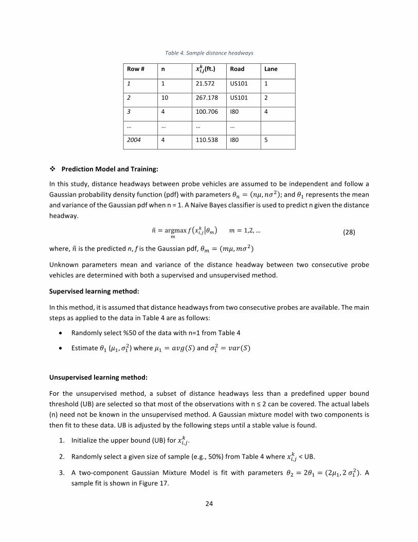
Table4.Sampledistanceheadways

Row# n 𝒙𝒊,𝒋𝒌 (ft.) Road Lane

1 1 21.572 US101 1

2 10 267.178 US101 2

3 4 100.706 I80 4

… … … …

2004 4 110.538 I80 5

v PredictionModelandTraining:

Inthisstudy,distanceheadwaysbetweenprobevehiclesareassumedtobeindependentandfollowaGaussianprobabilitydensityfunction(pdf)withparameters𝜃M = 𝑛𝜇, 𝑛𝜎F ;and𝜃ErepresentsthemeanandvarianceoftheGaussianpdfwhenn=1.ANaïveBayesclassifierisusedtopredictngiventhedistanceheadway.

𝑛 = argmaxL

𝑓 𝑥C,D" 𝜃L 𝑚 = 1,2, … (28)

where,𝑛isthepredictedn,fistheGaussianpdf,𝜃L = (𝑚𝜇,𝑚𝜎F)

Unknown parameters mean and variance of the distance headway between two consecutive probevehiclesaredeterminedwithbothasupervisedandunsupervisedmethod.

Supervisedlearningmethod:

Inthismethod,itisassumedthatdistanceheadwaysfromtwoconsecutiveprobesareavailable.ThemainstepsasappliedtothedatainTable4areasfollows:

• Randomlyselect%50ofthedatawithn=1fromTable4

• Estimate𝜃E(𝜇E, 𝜎EF)where𝜇E = 𝑎𝑣𝑔(𝑆)and𝜎EF = 𝑣𝑎𝑟(𝑆)

Unsupervisedlearningmethod:

For the unsupervised method, a subset of distance headways less than a predefined upper boundthreshold(UB)areselectedsothatmostoftheobservationswithn≤2canbecovered.Theactuallabels(n)neednotbeknownintheunsupervisedmethod.AGaussianmixturemodelwithtwocomponentsisthenfittothesedata.UBisadjustedbythefollowingstepsuntilastablevalueisfound.

1. Initializetheupperbound(UB)for𝑥C,D" .

2. Randomlyselectagivensizeofsample(e.g.,50%)fromTable4where𝑥C,D" <UB.

3. A two-component Gaussian Mixture Model is fit with parameters 𝜃F = 2𝜃E = (2𝜇E, 2𝜎EF). AsamplefitisshowninFigure17.

25

4. Theupperboundisupdatedtobethreestandarddeviationslargerthanthesecondmean:𝑈𝐵 =2𝜇E + 3 2𝜎EF

5. Steps2-4arerepeateduntilUBconverges.UBconvergesbetween10-20steps.

Figure17.AtwocomponentGaussianmixturemodeltofitthedata

v Results:

Supervisedandunsupervisedmethodsare appliedon the testdata topredictunobservednumberofvehiclesbetweenprobevehiclesbyestimatingthetwomodelparameters(𝜇E, 𝜎EF).ResultsareinFigure18below.Pleasenotethatdatausedfortrainingisexcludedinthegraphs.

Forthesupervisedmethod,50%ofalldistanceheadwaysforwhichn=1areusedfortrainingandrestisusedfortesting.Forn=1,thereareatotalof230samplesinthedata.Since115ofthemareusedformodeltraining,theyarenotincludedinthetopchartofFigure18.Hence,the115samplesonthefirstbar.Fortheunsupervisedmethod,samplesareselectedbasedontheUBcriterionasdiscussedbefore.Mostoftherandomsamplefortraininginthiscasecomesfromeithern=1orn=2conditionswhile11datapoints(198-187=11)arefromn=3.TheGMMmodelisthenfittothismixedsampleofpointstoestimatethemodelparameters.TheresultsshowninFigure18arefortheremainingdatapoints(i.e.,training data not included). From Figure 18, we can see that supervised and unsupervised methodsperformed similar. Horizontal axes show the unobserved number of vehicles between probes. Thenumberaboveeachbarshowsnumberofavailabledatafortestingcorrespondington.Thenumbersinwhiteareasrepresentcorrectprediction,whereasnumbersingrayareasrepresentunderpredictions(i.e.,𝑛 = 𝑛 − 1)oroverpredictions(i.e.,𝑛 = 𝑛 + 1).Inveryfewinstances,theover/under-predictionsareby±2,whichareindicatedbyredshading.TheBluelinesshowpredictionaccuracywhichiscalculatedbynumbersinwhiteareadividedbythecorrespondingsamplesize(numbersabovebars).

26

Figure18.Accuracyofthesupervisedandunsupervisedlearningmethodsappliedtothedistanceheadwaydata.

v Estimatingmacroscopictrafficdensity:

Trafficdensityiscalculatedbydividingtheprediction𝑛byheadwaydistance𝑥C,D" whichis𝑛/𝑥C,D

" .Accuracyofthisapproachiscomputedbythefollowingerrormeasure:

𝜀 =𝑛𝑥 −

𝑛𝑥

𝑛𝑥

∗ 100 (29)

Wheresubscriptsareomittedforsimplicity.Thisequationcanbewritteninasimplerwayby

𝜀 =𝑛 − 𝑛𝑛

∗ 100 (30)

Thiserrormeasure isusedtocalculatetheaccuracyof thetrafficdensitycalculation.Sinceweusedarandoma selection for trainingand testing.Eachmodel is trainedand tested30 times toaccount forvariations.Figure19showtheresultofthese30runs:theaverageestimated,actualdensitiesandthestandarddeviatione.Thebluelineshowsthestandarddeviationofe,thegreenandredonesshowtheactualandestimatedaveragedensities,respectively.Themacroscopicdensityisexpectedtobehighdueto thedatacoming fromstop-and-goordense trafficconditionsandFigure19showsthesameresultexceptthefirstbinwhereheadwayislessthan20ft.Standarddeviationoferrorforthefirstbiniszerosinceunrealisticsmallheadwayswhenx<20ftresultsinbothnand𝑛tobe1.Forheadwayslargerthan

27

20ft,standarddeviationoferrorstartshighanddecreasesasheadwayornincreases.WhileaccuracyofpredictingndecreaseswithincreasingninFigure18.

Figure19.Accuracyforsupervisedandunsupervisedmethods.Theresultsof30trialsareaggregatedbydistanceheadwaysbins

inincrementsof20ft.

Inthisstudy,numberofvehiclesbetweenprobevehiclesareestimatedusingdistanceinformationbetweenprobevehicles.NaïveBayesmodelwithGaussianpdfsareusedandtheirparametersareestimatedwithasupervisedandunsupervisedmethod.ThesemethodsaretestedwithNGSIMtrajectorydataandresultedingoodpredictionresultswithaccuracyof±1vehiclealmostalways.Later,predictednumberisusedtocalculatetrafficdensitybytheequation30.FromFigure19,wecanseethatmodelscanbeusedtocalculatemacroscopictrafficdensity.Accuracyincreasesasnumberofvehiclesordistanceheadwayincreases.Thisworkproposestwodifferentmethodsfortrafficflowparameterestimationfromprobevehicletrajectory.ThisworkwillbeextendedusingLIDARdata.

28

6. Conclusions:Inthisproject,authorsdevelopedmodelsandalgorithmsfortrafficflowparametersestimationfrom3DLIDARdataproblem.Authorsaddressedtheresearchobjectivesoftheproject:LIDARdataiscollectedunderdifferentconditionsonurbanandfreewayroads,vehiclesareclassifiedbasedontheirsizes,vehiclesaretrackedandtheirtrajectoriesareextractedandmicroscopicandmacroscopictrafficflowparametersarecalculatedfromvehicletrajectories.Wesuccessfullyappliedourmethodsonthedatawecollectedwithourvehicleonurbanandfreewayroads.DetectedvehiclesareclassifiedbasedontheirgeometryandthentheyareprocessedbyatrackingsystemconsistingofKalmanFilterwithHungarianAlgorithmfordataassociation.Usingthetrackinginformation,weconstructedvehicletrajectorieswhichhavevaluableinformationaboutthetrafficstatealongthedatacollectionpath.Then,collectedvehicletrajectoriesareusedinacar-followingmodelstopredictmissingdatapointsintrajectories.ThismethodgaveverysatisfactoryresultswhenappliedonknowntrajectoriesfromLIDARandNGSIMdatasets.Itisalsodemonstratedthattrafficdensitycanbeestimatedaccuratelyundercongestedconditionsusingasmallsampleofprobevehiclesinthetrafficstream.

7. References:

[1] J.C.Herrera,D.Work,R.Herring,J.Ban,Q.Jacobson,andA.Bayen.“EvaluationoftrafficdataobtainedviaGPS-enabledmobilephones:theMobileCenturyexperiment,”TransportationResearchPartC,2009

[2] M.BrackstoneandM.McDonald,"DynamicBehaviouralDataCollectionUsinganInstrumentedVehicle,"Transp.Res.Rec.,vol.1689,pp.9-17,1999.

[3] Goodall,N.,B.Smith,andB.Park.“MicroscopicEstimationofFreewayVehiclePositionsUsingMobileSensors”,InTRB91stAnnualMeeting.2011.

[4] http://velodynelidar.com/[5] D.Pfeiffer,U.Franke,Efficientrepresentationoftrafficscenesbymeansofdynamicstixels,in:

IntelligentVehiclesSymposium(IV),2010IEEE,pp.217–224,2010[6] A.Broggi,S.Cattani,M.Patander,M.Sabbatelli,P.Zani,Afull-3dvoxel-baseddynamicobstacle

detectionforurbanscenariousingstereovision,in:IntelligentTransportationSystems-(ITSC),201316thInternationalIEEEConferenceon,pp.71–76,2013

[7] A.Azim,O.Aycard,Layer-basedsupervisedclassificationofmovingobjectsinoutdoordynamicenvironmentusing3dlaserscanner,in:IntelligentVehiclesSymposiumProceedings,2014IEEE,pp.1408–1414,2014

[8] M.Oliveira,V.Santos,A.Sappa,P.Dias,Scenerepresentationsforautonomousdriving:anapproachbasedonpolygonalprimitives,in:2ndIberianRoboticsConference,2015

[9] F.Oniga,S.Nedevschi,Processingdensestereodatausingelevationmaps:Roadsurface,trafficisle,andobstacledetection,VehicularTechnology,IEEETransactionson59(3)(2010)1172–1182.

[10] A.Asvadi,P.Peixoto,U.Nunes,Detectionandtrackingofmovingobjectsusing2.5dmotiongrids,in:IntelligentTransportationSystems(ITSC),2015IEEE18thInternationalConferenceon,2015,pp.788–793.

[11] M.Ester,H.Kriegel,J.Sander,andX.Xu,“Adensity-basedalgorithmfordiscoveringclustersinlargespatialdatabaseswithnoise,”inProc.2ndInt.Conf.KnowledgeDiscoveryandDataMining(KDD’96),pp.226–231,1996

29

[12] R.E.Kalman.“Anewapproachtolinearfilteringandpredictionproblems”InTrans.ASMEVJ.BasicEng,pagesser.D,vol.82,pp.35-45,1960

[13] Z.Luo,S.HabibiandM.V.Mohrenschildt,“LiDARBasedRealTimeMultipleVehicleDetectionandTracking”,InternationalJournalofComputer,Electrical,Automation,ControlandInformationEngineering,vol.10,pp.1125-1132,2016

[14] A.Macaveiu,A.Campeanu,andI.Nafornita,“Kalman-basedtrackerformultipleradartargets”inCOMM2014InternationalConferenceonCommunications,Bucharest,Romania,2014.

[15] H.W.Kuhn,“TheHungarianmethodfortheassignmentproblem”,NavalResearchLogistics,Vol.52,pp.7-21,2005.

[16] C.Sazara,R.V.Nezafat,M.Cetin,“Offlinereconstructionofmissingvehicletrajectorydatafrom3DLIDAR”,IntelligentVehiclesSymposium(IV),2017IEEE,pp.792-797,2017

[17] FHWA.(2017,9/20/2017).NextGenerationSimulation(NGSIM).Available:https://ops.fhwa.dot.gov/trafficanalysistools/ngsim.htm

[18] M.TreiberandA.Kesting,Trafficflowdynamics:data,modelsandsimulation.Heidelberg;NewYork:Springer,2013.

[19] D.H.M.Treiber,“Congestedtrafficstatesinempiricalobservationsandmicroscopicsimulations,”PhysRev.E62,1805,2000.

[20] PipesLA,“Anoperationalanalysisoftrafficdynamics”JApplPhys24(3):pp.274–281,1953[21] Newell,G.,Asimplifiedcar-followingtheory:alowerordermodel.TransportationResearchPartB,

36,195–205,2002[22] M.CetinandK.A.Anuar,“UsingProbeVehicleTrajectoriesinStop-and-GoWavesforInferring

UnobservedVehicles”5thIEEEInternationalConferenceonModelsandTechnologiesforITS,Naples,Italy,June26-282017.

[23] G.ComertandM.Cetin,"Queuelengthestimationfromprobevehiclelocationandtheimpactsofsamplesize,"EuropeanJournalofOperationalResearch,vol.197,pp.196-202,2009.

[24] G.ComertandM.Cetin,"AnalyticalevaluationoftheerrorinqueuelengthestimationattrafficsignalsfromprobevehicledData,"IEEETransactionsonIntelligentTransportationSystems,vol.12,pp.563-573,2011.

[25] J.Anderson,B.Ran,J.Jin,X.Qin,andY.Cheng,"Cycle-by-CycleQueueLengthEstimationforSignalizedIntersectionsUsingSampledTrajectoryData,"TransportationResearchRecord:JournaloftheTransportationResearchBoard,vol.2257,pp.87-94,2011.

[26] Q.Cai,Z.Wang,L.Zheng,B.Wu,andY.Wang,"ShockWaveApproachforEstimatingQueueLengthatSignalizedIntersectionsbyFusingDatafromPointandMobileSensors,"TransportationResearchRecord:JournaloftheTransportationResearchBoard,vol.2422,pp.79-87,2014.

[27] M.Cetin,"Estimatingqueuedynamicsatsignalizedintersectionsfromprobevehicledata,"TransportationResearchRecord:JournaloftheTransportationResearchBoard,vol.2315,pp.164-172,2012.

[28] S.Y.R.Rompis,M.Cetin,andF.Habtemichael,"ProbeVehicleLaneIdentificationforQueueLengthEstimationatIntersections,"JournalofIntelligentTransportationSystems,pp.0-0,2017.