Fluorescence Dosimetry for Photodynamic Therapy via an Interstitial Rotary Fiber Probe

A Thesis Submitted to the Faculty

in partial fulfillment of the requirements for the degree of

Master of Science

by

TIMOTHY D. MONAHAN

Thayer School of Engineering Dartmouth College

Hanover, New Hampshire

March 2008

Examining Committee: _____________________________

Brian Pogue Chairman

_____________________________ Jack Hoopes

_____________________________ Shudong Jiang

________________________ Charles K. Barlowe Dean of Graduate Studies © 2008 Trustees of Dartmouth College _____________________________

Timothy Monahan

ii

Thayer School of Engineering Dartmouth College

“Fluorescence Dosimetry for Photodynamic Therapy

via an Interstitial Rotary Fiber Probe”

Timothy D. Monahan

Master of Science

Committee

Brian Pogue Jack Hoopes

Shudong Jiang

Abstract

In photodynamic therapy (PDT) a photosensitive drug is administered to a patient

and then activated with a specified light dose. As in most therapies, the drug delivery is

known to be heterogeneous and in previous studies PDT has been shown to benefit from

pre-treatment measurement of this drug uptake[1]. Despite these published results most

research in PDT focuses on the drug development and validation, and full photosensitizer

dosimetry remains underdeveloped in PDT. Sampling of drug distribution in tissue has

always been a problematic issue, and in PDT the distribution is known to be

heterogeneous[2]. In this work, the limitations of pre-treatment dosimetry were studied

using both simulations and experiments, and a new dosimeter utilizing a novel rotating

probe design was designed, built, and evaluated.

The new dosimeter was based on an existing design which was used as a

reference point while testing the redesigned dosimeter. The redesigned dosimeter for

interstitial use was more than 4 times more sensitive than the existing dosimeter for

iii

surface measurements due to a combination of design improvements and the use of better

components.

The rotating probe configuration allows multiple measurements to be taken during

insertion or pull back in tissue, and circumferentially around the tracks. The effective

measurement depth is limited to a few hundred microns. The design of the optical fiber

used in the interstitial probe limited sensitivity; the probe cannot determine the direction

of the fluorescence in a medium with the optical properties found in vivo but it is possible

that a different design could improve sensitivity. Due to geometric and fiber optical

constraints, the new probe's sensitivity could be an order of magnitude less than that of a

more traditional surface probe.

In addition to limits in measurement depth and sensitivity, the rotating probe is

more fragile and requires greater care of use. Building on the work in this thesis could

produce an interstitial probe that could aid researchers by giving additional information

about drug distributions in vivo along a vessel track or at large numbers of points in

tumor tissue.

iv

Preface

Throughout the course of this project many people have offered help, guidance

and advice. None have been as supportive, helpful, or knowledgeable as my advisor,

Brian Pogue. Without him, this project would not have been possible.

The members of the NIRfast group and the Thayer community in general were

always willing to help whenever I needed assistance. They offered a wealth of

experience, knowledge, and companionship throughout this project. Venkataramanan

Krishnaswamy offered insight into the optical portion of the system, and was a constant

sounding board for new ideas. His enthusiasm for research was contagious and was one

of the factors that helped keep my research moving. Most of the mouse experiments were

a part of a study being done by Kim Samkoe. Her willingness to incorporate my research

into her study made the pharmacokinetics study possible. Julia O’Hara and the

researchers and staff at the Animal Resource Center at the Dartmouth Hitchcock Medical

Center enabled the animal experiments in this project. Their experience with and

compassion for the animals in the facility was inspiring. It was a pleasure to know and

work with Colin Carpenter, Scott Davis, Summer Gibbs-Strauss, Shudong Jiang, Dax

Kepshire, Ashley Laughney, Zhiqui Li, Subhadra Srinivasan, Jia Wang, and Phaneendra

Yalavarthy.

The love and support of my fiancé and family has been a constant source of

motivation throughout this project. Without them and without their encouragement, this

work would not have been possible.

Funding for this work is from the National Cancer Institute PO1CA84203 and

NIH award #R01 CA109558.

v

Table of Contents Abstract ............................................................................................................................... ii Preface................................................................................................................................ iv Table of Contents................................................................................................................ v List of Figures .................................................................................................................... vi Introduction......................................................................................................................... 1

Overview......................................................................................................................... 1 Background..................................................................................................................... 1

Probe Design....................................................................................................................... 3 Fiber Design.................................................................................................................... 4 Mechanical Design.......................................................................................................... 8 Control Code Changes .................................................................................................. 11 Calibration..................................................................................................................... 12

New Dosimeter Design ..................................................................................................... 14 Code Updates ................................................................................................................ 15 Component Changes ..................................................................................................... 17 Design Changes ............................................................................................................ 18 Validation...................................................................................................................... 20

Fluorescence Quantum Yield and Oxygen ....................................................................... 23 Methodology................................................................................................................. 24 Results........................................................................................................................... 25 Discussion..................................................................................................................... 32

Phantom & Simulation Experiments ................................................................................ 33 Optical property simulation study................................................................................. 33 Phantom Studies............................................................................................................ 40

Mouse Experiments .......................................................................................................... 48 AsPC1 Pharmacokinetics Measured with the Surface Probe ....................................... 48 AsPC1 Pharmacokinetics Measured with the Interstitial Probe ................................... 54 Panc1 Pharmacokinetics Measured with the Surface Probe ......................................... 57

Conclusions....................................................................................................................... 60 Future Directions .............................................................................................................. 62 Appendix........................................................................................................................... 65

Dosimeter LabView Code............................................................................................. 65 Bibliography ..................................................................................................................... 68

vi

List of Figures Figure 1: The chemical structure of the benzoporphyrin monoacid ring a derivate, also known as verteporfin. Verteporfin is a product of QLT Inc (Canada). This image was taken from the QLT website. .............................................................................................. 2 Figure 2: Diagram of a total internal reflection off of the polished face of a side firing fiber. As can be seen in this diagram, the light exits the fiber through the curved surface of the fiber which causes a wide acceptance angle............................................................. 4 Figure 3: Fiber polishing pucks for polishing the fiber at various angles. From right to left the pucks are for polishing fibers at 45, 50, 55, and 60 degrees. ........................................ 5 Figure 4: Polishing a fiber using 1 μm grit polishing paper. The SMA connection is being polished in this image. At this stage the other end of the fiber has already been polished to 50 degrees. ...................................................................................................................... 5 Figure 5: Diagram of the experimental setup for the acceptance angle measurements. The red arrow indicates where the 635nm laser illuminated the fiber. The laser spot was much larger than the fiber tip, so vibrations caused by the stepper motor did not move the fiber tip outside of the laser spot. The curved yellow arrow indicates the rotation of the fiber while the measurements were taken. In this image the hollow fiber is in place................. 6 Figure 6: Measured intensity at the output end of the fiber with 630 nm diode laser light aimed at the tip of the fiber. For these measurements the fiber was rotated through all angles. The measurement was done for the bare fiber (a) and fiber inside the glass fiber (b), and acceptance angles were estimated from this data. ................................................. 7 Figure 7: Diagram of the hollow fiber, side firing fiber, and the needle at the tip of the interstitial probe. ................................................................................................................. 8 Figure 8: A Pro-Engineer rendering of the rotating probe. The needle, outer fiber support, gearbox, fiber optic rotary joint, stepper motor, and gears are shown in this image. Not shown are the inner fiber support, and the gear adaptor for the rotary joint. The rotating fiber was held by the inner fiber support, and inserted through a syringe needle at the end. This geometry allowed for multiple measurements around the fiber tip instead of the single point measurement of the surface probe................................................................... 9 Figure 9: Exploded view of rotating probe. The needle, outer fiber support, inner fiber support, gearbox, fiber optic rotary joint, gear adaptor for the fiber optic rotary joint, stepper motor, and gears are shown in this image. ........................................................... 10 Figure 10: Diagrams of the needle extended to cover the fiber (a) and retracted to expose the fiber (b). This design allows the needle to be extended while the probe is inserted into the tissue, and then the needle can be retracted to expose the fiber. This process prevents loads on the fiber during the insertion process, and protects the fiber when not in use. .. 11 Figure 11: Diagram showing how the probe is inserted into tissue. First, the needle is extended so the fiber is covered (b), and then inserted into the tissue (b). Once the probe is in the correct position, the needle is retracted to expose the fiber (c). In this picture the fiber is shown with the hollow fiber in place.................................................................... 11 Figure 12: Block diagrams of Aurora_one_sample_nogainchange_USBversion.vi (a) and Aurora_continuous_sample_nogainchange_USBversion.vi (b). As is mentioned in a later code changes section in the dosimeter design, the averaging routine for (b) is different

vii

than used in (a). In addition, (b) returns an averaged data set with 100 values in addition to the mean of the data set................................................................................................. 12 Figure 13: Photobleaching of fluorescence in side firing fiber used in the interstitial probe. These measurements were taken with the interstitial probe in free space in a dark room. With that experimental setup the results without bleaching would be a constant measurement, but in this case a large degree of variability can be seen. The photobleaching effect appeared to be temporary which made calibrating the probe to eliminate the effect of this phenomenon difficult. ............................................................ 14 Figure 14: Picture of the surface dosimeter (Aurora Optics, Inc.). The filter eliminates any excitation light that may have entered the detector fibers and ensures that the measured signal is from fluorescence. The filter and collimator are connected to the secondary collimator, and signals are measured with the photomultiplier tube and recorded by the data acquisition board. The laser control board is used to provide a 200 Hz square wave to the laser, and is activated by the data acquisition board. ................... 15 Figure 15: Screenshot of the data acquisition portion of the LabView control software. This software allows users to pick different averaging methods for the rotating measurements, as well as an option to take measurements without rotation. The small graph in the center shows the results of measurements without rotation, while the much larger graph on the right shows the results with rotation.................................................. 16 Figure 16: Measurements on the both the black calibration standard (a) and the fluorescent calibration standard (b). These 10 samples give a comparison of various schemes for averaging raw data from the dosimeter. The ideal averaging method will produce a straight line, as all 10 measurements in each plot were taken from the same sample. Each of the 4 plotted lines is a different averaging scheme. The “Peak to Peak” method (blue line) are the difference between the maximum and minimum values in the data set. The “Peak to Peak” method is greatly affected by noise, especially when the measured intensity is low (a). These results show that the “Average Amplitude” (red line) method is clearly preferable.............................................................................................. 17 Figure 17: Exploded Pro-Engineer rendering of the shutter box with photomultiplier tube and shutter. The shutter box is made up of the gray components. Several important features have been labeled including the shutter, an example of the rebated joints used to prevent stray light from entering the system, the location of the threaded hole for the optical tube, adaptor, and collimator assembly, the photomultiplier tube window, and the photomultiplier tube.......................................................................................................... 19 Figure 18: Dosimeter sensitivity study done with a mixture of 0.0002% ink, .2% Intralipid and various concentrations of BPD-MA molecule in phosphate buffered saline solution. The surface probe had 6 detectors around each source, and seven source and detector clusters. Measurements were taken with the surface probe attached to both the surface dosimeter and the interstitial dosimeter, and with the interstitial probe attached to the interstitial dosimeter. The response to changing concentration of BPD-MA is linear for both dosimeters. The interstitial probe has limited sensitivity compared to the surface probe, which is likely due to the fluorescence of the fibers in the interstitial probe. ....... 22 Figure 19: Results from the DPBS experiment. Yeast was added to the solution at time zero. De-oxygenation occurred and was measured using the chemical microsensor. The fluorescence was measured using the surface dosimeter. These results show no correlation between measured oxygen levels and fluorescence. ...................................... 27

viii

Figure 20: Results from the blood, Intralipid and PBS experiment. Yeast was added to the solution at time zero. De-oxygenation occurred and was measured using the chemical microsensor and the ischemia detector. The fluorescence was measured using the surface dosimeter. These results show a slope near zero for the fluorescence, indicating no correlation with oxygenation. ........................................................................................... 28 Figure 21: Comparison of the oxygen saturation detector measurement with the oxygenation measurement from the chemical microsensor.............................................. 30 Figure 22: Results from the blood, Intralipid and DPBS experiment. Yeast was added to the solution at time zero. De-oxygenation occurred and was measured using the chemical microsensor and the ischemia detector. The fluorescence was measured using the Aurora Dosimeter. A negative slope can be seen in the fluorescence measurements as time increases. This slope can be attributed to the photo bleaching effect. These results explain why a 4% increase in fluorescence was not seen in the previous experiments. ............... 31 Figure 23: Screenshot of the difference between pre and post contrast CT scans. The pancreas has been segmented in this image, and can be seen as the tan sections, and as the tan object in the 3D rendering of areas with high perfusion. The patient moved between the pre and post contrast scans due to breathing, and as a result the ribs show up as having large amounts of blood flow. The difference image was used to estimate blood flow, which was then used to estimate the heterogeneities in the optical properties of the tissue. ................................................................................................................................ 35 Figure 24: Screenshot of mesh superimposed over the difference of pre and post contrast CT scans. The difference of the scans was used to estimate blood volume, and that estimate was used to calculate the heterogeneities in optical properties. These properties were assigned to the nodes of the mesh, and were used in the forward finite element simulations shown below.................................................................................................. 36 Figure 25: Plot of difference between fluence calculated from heterogeneous optical properties and a prediction using a homogeneous assumption. The simulations were done with a finite element method forward simulation using optical properties calculated from estimated blood concentrations. Three source locations were chosen, one near the center of the pancreas and two close to an artery. The samples near the artery are in different locations, so the results should be different. The difference in the homogeneous results and the heterogeneous results at each node were calculated. This results in multiple differences at each distance so error bars were used to show the standard deviation of this difference. These results are part of a simulation study to determine which assumptions can be made about optical properties in vivo.................................................................... 37 Figure 26: Plot of difference between a heterogeneous prediction where the exact optical properties are not registered correctly spatially. In this case the offset was 1 cm. The simulations were done with a finite element method forward simulation using optical properties calculated from estimated blood concentrations. Three source locations were chosen, one near the center of the pancreas and two close to an artery. The samples near the artery are in different locations, so the results should be different. The difference in the homogeneous results and the heterogeneous results at each node were calculated. This results in multiple differences at each distance so error bars were used to show the standard deviation of this difference. These results are part of a simulation study to determine which assumptions can be made about optical properties in vivo. .................. 38

ix

Figure 27: This plot shows the difference between a homogeneous prediction where the optical properties are not registered correctly and a heterogeneous model. In this case the offset was 1 cm. The simulations were done with a finite element method forward simulation using optical properties calculated from estimated blood concentrations. Three source locations were chosen, one near the center of the pancreas and two close to an artery. The samples near the artery are in different locations, so the results should be different. The difference in the homogeneous results and the heterogeneous results at each node were calculated. This results in multiple differences at each distance so error bars were used to show the standard deviation of this difference. These results are part of a simulation study to determine which assumptions can be made about optical properties in vivo. The results of this graph show that there is a large difference between the prediction and the actual fluence, but that it is similar to that of the heterogeneous prediction with the same coregistration error. These results indicated that there is no advantage to using heterogeneous optical properties if there were coregistration errors. 39 Figure 28: Setup of experiment to measure the effect of distance on fluorescence intensity. The interstitial probe is attached to a post (not shown) screwed into the optical table. The foam acted as the fluorescent sample, and was moved using the micron stage (upper right corner of picture). Measurements were taken at various separations between the fiber and the fluorescent sample. ................................................................................ 41 Figure 29: Plot of measured fluorescence intensity at various distances from the source. As can be seen in this plot, the intensity decays exponentially and the probe has the greatest sensitivity to measurements taken less than 1 mm from the fluorescent object. The fluorescence in the fiber of the interstitial probe adds a significant amount of noise to the measurement, but the general trend in the data is still clear. ...................................... 42 Figure 30: Setup of experiment to measure the effect of distance on detection of the origin of fluorescence. The interstitial probe is attached to a post (not shown) screwed into the optical table. The foam acts as the fluorescent sample, and is moved using the micron stage (upper right corner of picture). Measurements were taken while the fiber rotated at various separations between the fiber and the fluorescent sample. This picture was taken with the 0.2% Intralipid and 1% blood phantom being added to the cup. ....... 43 Figure 31: Plot of the intensity at different rotation angles over distance for the interstitial probe. The fluorescent object was located at 180 degrees. These results with 1% Intralipid and 1% blood show that the probe cannot detect the direction of fluorescence when optical properties are similar to those found in vivo. Also clear from this plot is that most of the sensitivity to in the measurement is at distances less than 1 mm. ................. 44 Figure 32: Plot of the intensity at all rotation angles over distance for the interstitial probe. The fluorescent object was located at 180 degrees. These results with 1% Intralipid and 1% blood show that the probe cannot detect the direction of fluorescence when optical properties are similar to those found in vivo. Also clear from this plot is that most of the sensitivity to in the measurement is at distances less than 1 mm. ................. 45 Figure 33: Plot of the intensity at different rotation angles over distance for the interstitial probe. The fluorescent object was located at 180 degrees. These results with 0.2% Intralipid and 1% blood show that the probe can detect the direction of fluorescence after approximately 1 mm when there is less scattering than found in the in vivo case. Also clear from this plot is that most of the sensitivity to in the measurement is at distances less than 1 mm. ................................................................................................................. 46

x

Figure 34: Plot of the intensity at all rotation angles over distance for the interstitial probe. The fluorescent object was located at 180 degrees. These results with 0.2% Intralipid and 1% blood show that the probe can detect the direction of fluorescence after approximately 1 mm when there is less scattering than found in the in vivo case. Also clear from this plot is that most of the sensitivity to in the measurement is at distances less than 1 mm. ................................................................................................................. 47 Figure 35: Subcutaneous AsPC1 tumor (a) and orthotopic AsPC1 tumor (b). These images were taken by Venkataramanan Krishnaswamy (a) and Kim Samkoe (b). The tumors were allowed to grow until they measured approximately 6mm, as assessed with calipers for the subcutaneous model and measured with 3T MR system for the orthotopic model................................................................................................................................. 49 Figure 36: Subcutaneous AsPC1 tumor pharmacokinetics were measured with the surface dosimeter using the surface probe. In both cases, injection was at time 0. Only two mice were measured this way, so both plots represent individual animals instead of averages. Both mice were injected with at a 1mg/kg dose of BPD-MA molecule. The tail of mouse (a) was damaged so only half a dose could be given in the tail vein; the other half dose was injected intra-peritoneal. Pre-injection measurements are available for the second data set (b), and indicate pre-injection levels of fluorescence were near 0.7 (same units as the measurements). ........................................................................................................... 51 Figure 37: An example of a bad injection of verteporfin. Verteporfin injection occurred at time 0. Notice the lack of accumulation in the tumor and the slow increase of fluorescence in the liver. ................................................................................................... 52 Figure 38: Mean of the normalized results from the orthotopic AsPC1 tumor study (n=4 animals). Verteporfin injection occurred at time 0, and only good injection animals were used in this analysis. Each data set was normalized so the maximum measurement before averaging was set to one. The error bars shown are the standard deviation between animals, which is why the measurements are below 1. This was done to prevent variations in the concentration of the drug from altering the results in an averaged study. See Figure 37 for an example of a bad injection. Measurements were taken when the tumors were approximately 6 mm in size. ........................................................................ 53 Figure 39: Pharmacokinetics of verteporfin injected into a subcutaneous AsPC1 tumor grown on the right hind leg of a SCID mouse measured with the interstitial probe with the surface dosimeter. Verteporfin injection occurred at time 0, and measurements were taken every minute after injection. Measurements were taken at all angles. A relatively homogeneous fluorescence measurement was observed, with two fluorescence peaks at 35 and 85 minutes. ............................................................................................................ 56 Figure 40: Mean of the normalized results from the orthotopic Panc1 tumor study (n=4 animals). Verteporfin injection occurred at time 0. Each data set was normalized so the maximum measurement before averaging was set to one. The error bars shown are the standard deviation between animals, which is why the measurements are below 1. This was done to prevent variations in the concentration of the drug from altering the results in an averaged study. It appears that the fluorescence increase begins before time 0, part of this effect is that measurements are not taken while the drug is injected so the last pre-injection measurement can be some time before the first post injection measurement. The injection times were recorded to the minute, so there may be nearly a full minute of error

xi

from the lack of precision in that measurement. Measurements were taken when the tumors were approximately 6 mm in size. ........................................................................ 59 Figure 41: Screenshot of the LabView calibration routine as seen by the user. The background and fluorescence reference buttons are the two buttons in the lower left hand corner of the image. The red oval in the bottom center of the image indicates that the calibration is not complete, once the calibration has been completed the oval will turn green and allow the user to enter the measurement screen. In the upper center is a button to load previous calibrations. ............................................................................................ 65

1

Introduction

Overview

Interest in photodynamic therapy (PDT) as a tumor treatment has been strong

since initial studies with hematoporphyrin in the late 1970’s. Since then experimental

PDT treatments have included skin lesions, esophageal lesions, head and neck lesions,

intra-ocular lesions, gastric cancers, gynecological cancers and rectal cancers[3]. Many of

these studies have had promising results. Some studies, including one done with

pancreatic cancer in 2002 have had a large degree of variation in the results of the

therapy[4]. In that study the authors identified dosimetry as a potential method of

reducing the variability in the treatment.

Despite these published results most research in PDT focuses on drug

development and validation, and photosensitizer dosimetry remains underdeveloped in

PDT. Sampling of drug distribution in tissue has always been a problematic issue, and in

PDT the distribution is known to be heterogeneous. In this work, the limitations of pre-

treatment dosimetry were studied using both simulations and experiments, and a new

dosimeter utilizing a novel rotating probe design was designed, built, and evaluated.

Background

Photodynamic therapy (PDT) is a cancer treatment that uses light and a

photosensitive drug to excite singlet oxygen and free radicals in tumor tissue. The excited

singlet oxygen influences multiple cell death pathways to cause tissue necrosis [5]. The

beneficial effects of photodynamic therapy include widespread apoptosis in tumor

2

regions with high specificity to tumor cells, neovasculature shutdown, and

immunological responses which can result in tissue wide effects beyond that estimated by

the singlet oxygen dose [6].

Figure 1: The chemical structure of the benzoporphyrin monoacid ring a derivate, also known as verteporfin. Verteporfin is a product of QLT Inc (Canada) [7].

Photosensitive drugs, also know as photosensitizers, are molecules that are

excited to a singlet state through the absorption of light. Once in a singlet state, these

molecules will relax to the ground state by releasing a fluorescent photon or excitation of

oxygen through intersystem crossing after relaxing to the triplet state[3]. A small number

of the photosensitizers currently used for PDT include photofrin, protoporphyrin IX, m-

THPC, and BPD-MA[3].

Photosensitizers have been shown to preferentially accumulate in some tumors.

Immediately after injection the photosensitizer is uniformly distributed in the vasculature

and enters tissue through perfusion and diffusion. Preferential accumulation occurs due to

the leaky nature of the vasculature found in tumors, and the slower clearance rate of the

tumor compared to normal tissue[8-12]. Treatment plans for PDT often include a

significant waiting period between injection of photosensitizer and the administration of

light to allow for the preferential accumulation of the photosensitizer to occur.

The uptake of the photosensitizer varies from patient to patient, so the drug levels

in the treatment area cannot be accurately calculated based on the amount administered to

a patient[13]. Attempts to use these calculations instead of measurements of drug

concentration can lead to a large degree of variability in tumor response.

3

Current pretreatment planning focuses on optimizing the light delivery to achieve

a uniform fluence in the treatment area and to minimize the fluence in the surrounding

tissues. These calculations do not attempt to measure or correct for heterogeneous

distributions of photosensitizer in the treatment area. The accuracy of these calculations

depends on knowledge of the absorption and scattering properties of the tissue, which are

difficult to measure accurately in vivo.

In the studies that have attempted to quantify drug concentrations before

treatment, one solution has been to calculate the drug concentrations based on

fluorescence measurements taken in the area[3]. These measurements are typically made

using surface probes that consist of some number of source and detector fibers. The drug

concentrations are then typically calculated with the assumptions that fluorescence

quantum yield is constant and that the optical properties are uniform.

Probe Design

The existing surface probe is made from a cluster of individual fiber optics with

separate source and detector channels; this design for surface measurements of

fluorescence in tissue was used for validation of the interstitial dosimeter electronics. It

consists of seven source/detector clusters, with each cluster containing one 100 micron

source fiber surrounded by six 100 micron detector fibers. The source and detector fibers

are 100 microns apart center to center, and the individual clusters are spaced apart by 700

microns to allow minimal crosstalk between clusters probing the tissue. The dosimeter

design has been discussed in several previous papers, and this geometry allows a

microsampling approach to record the signal from 100-200 micron sized regions of tissue

4

that minimizes the effect of varying optical properties on fluorescence measurements[2,

14-16].

The project examines a novel interstitial probe design for PDT dosimetry. The

probe designed for this project uses a single 100 micron rotating side firing fiber for both

delivery of excitation light and detecting the fluorescent signal. This new approach

allows for orthogonal measurements at all angles around the fiber instead of a single

measurement directly in front of the fiber tip.

Fiber Design

There are many options for creating side firing fibers. These options include

attaching optical components such as prisms or mirrors to the end of a fiber and polishing

the fiber at an angle. Attaching optical components to the end of a small fiber is difficult

and requires specialized equipment which makes these components expensive. Fiber

polishing can be done at Thayer, and if an appropriate angle is chosen a total internal

reflection can be achieved. Polishing the fiber was chosen as the best option for the initial

prototype. A 100 micron fiber was used for the side firing fiber (AFS 105/125y, Thorlabs

Inc., Newton, NJ).

Figure 2: Diagram of a total internal reflection off of the polished face of a side firing fiber. As can be seen in this diagram, the light exits the fiber through the curved surface of the fiber which causes a wide acceptance angle.

5

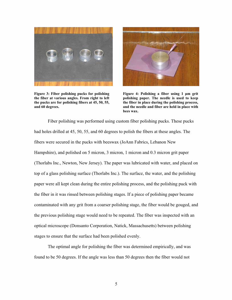
Figure 3: Fiber polishing pucks for polishing the fiber at various angles. From right to left the pucks are for polishing fibers at 45, 50, 55, and 60 degrees.

Figure 4: Polishing a fiber using 1 μm grit polishing paper. The needle is used to keep the fiber in place during the polishing process, and the needle and fiber are held in place with bees wax.

Fiber polishing was performed using custom fiber polishing pucks. These pucks

had holes drilled at 45, 50, 55, and 60 degrees to polish the fibers at these angles. The

fibers were secured in the pucks with beeswax (JoAnn Fabrics, Lebanon New

Hampshire), and polished on 5 micron, 3 micron, 1 micron and 0.3 micron grit paper

(Thorlabs Inc., Newton, New Jersey). The paper was lubricated with water, and placed on

top of a glass polishing surface (Thorlabs Inc.). The surface, the water, and the polishing

paper were all kept clean during the entire polishing process, and the polishing puck with

the fiber in it was rinsed between polishing stages. If a piece of polishing paper became

contaminated with any grit from a coarser polishing stage, the fiber would be gouged, and

the previous polishing stage would need to be repeated. The fiber was inspected with an

optical microscope (Donsanto Corporation, Natick, Massachusetts) between polishing

stages to ensure that the surface had been polished evenly.

The optimal angle for polishing the fiber was determined empirically, and was

found to be 50 degrees. If the angle was less than 50 degrees then the fiber would not

6

achieve a total internal reflection, and if the angle was greater than 50 degrees the

intensity of the light transmitted through the fiber decreased.

In addition, it was found that the fiber buffer layer absorbed some of the light

from the fiber. When the buffer layer was removed, the more light was transmitted

through the fiber. Unfortunately, the fiber is far more delicate without the buffer layer

and is prone to breaking. The polymer buffer on the fiber could be removed mechanically

with a fiber stripper, but this did not work for the polymide buffer of the hollow fiber.

The polymide buffer layer was burned off, which can not be done after the fiber is

polished. It may be preferable to remove the buffer layer chemically, but this was not

attempted.

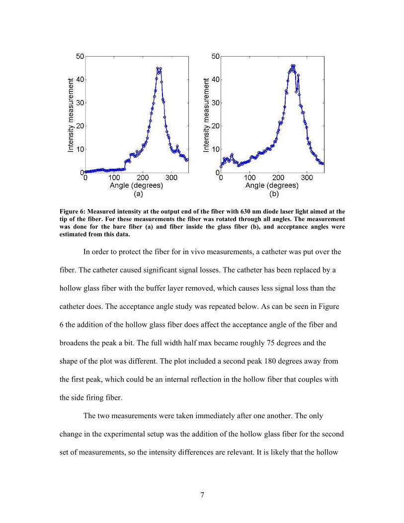
Figure 5: Diagram of the experimental setup for the acceptance angle measurements. The red arrow indicates where the 635nm laser illuminated the fiber. The laser spot was much larger than the fiber tip, so vibrations caused by the stepper motor did not move the fiber tip outside of the laser spot. The curved yellow arrow indicates the rotation of the fiber while the measurements were taken. In this image the hollow fiber is in place. Once the side firing fiber was made the new acceptance angle of the fiber was

tested. As can be seen in the plot below, the full width half max value of the side firing

fiber was roughly 50 degrees.

7

Figure 6: Measured intensity at the output end of the fiber with 630 nm diode laser light aimed at the tip of the fiber. For these measurements the fiber was rotated through all angles. The measurement was done for the bare fiber (a) and fiber inside the glass fiber (b), and acceptance angles were estimated from this data.

In order to protect the fiber for in vivo measurements, a catheter was put over the

fiber. The catheter caused significant signal losses. The catheter has been replaced by a

hollow glass fiber with the buffer layer removed, which causes less signal loss than the

catheter does. The acceptance angle study was repeated below. As can be seen in Figure

6 the addition of the hollow glass fiber does affect the acceptance angle of the fiber and

broadens the peak a bit. The full width half max became roughly 75 degrees and the

shape of the plot was different. The plot included a second peak 180 degrees away from

the first peak, which could be an internal reflection in the hollow fiber that couples with

the side firing fiber.

The two measurements were taken immediately after one another. The only

change in the experimental setup was the addition of the hollow glass fiber for the second

set of measurements, so the intensity differences are relevant. It is likely that the hollow

8

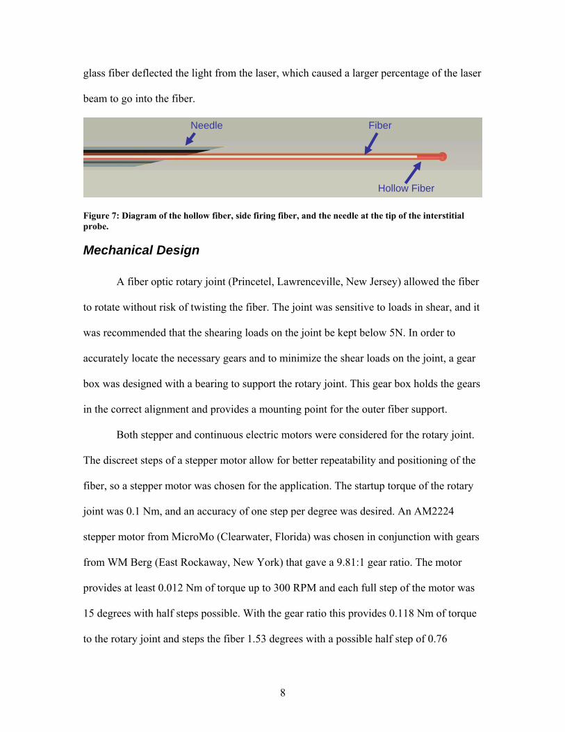
glass fiber deflected the light from the laser, which caused a larger percentage of the laser

beam to go into the fiber.

Figure 7: Diagram of the hollow fiber, side firing fiber, and the needle at the tip of the interstitial probe.

Mechanical Design

A fiber optic rotary joint (Princetel, Lawrenceville, New Jersey) allowed the fiber

to rotate without risk of twisting the fiber. The joint was sensitive to loads in shear, and it

was recommended that the shearing loads on the joint be kept below 5N. In order to

accurately locate the necessary gears and to minimize the shear loads on the joint, a gear

box was designed with a bearing to support the rotary joint. This gear box holds the gears

in the correct alignment and provides a mounting point for the outer fiber support.

Both stepper and continuous electric motors were considered for the rotary joint.

The discreet steps of a stepper motor allow for better repeatability and positioning of the

fiber, so a stepper motor was chosen for the application. The startup torque of the rotary

joint was 0.1 Nm, and an accuracy of one step per degree was desired. An AM2224

stepper motor from MicroMo (Clearwater, Florida) was chosen in conjunction with gears

from WM Berg (East Rockaway, New York) that gave a 9.81:1 gear ratio. The motor

provides at least 0.012 Nm of torque up to 300 RPM and each full step of the motor was

15 degrees with half steps possible. With the gear ratio this provides 0.118 Nm of torque

to the rotary joint and steps the fiber 1.53 degrees with a possible half step of 0.76

Needle Fiber

Hollow Fiber

9

degrees. The gears were connected to the rotary joint with a custom made adaptor, and

were aligned by the gearbox. The stepper motor was controlled with a AD VM M1S

controller provided by MicroMo and signals from a National Instruments (Austin, Texas)

USB 6009 data acquisition and control board.

Figure 8: A Pro-Engineer rendering of the rotating probe. The needle, outer fiber support, gearbox, fiber optic rotary joint, stepper motor, and gears are shown in this image. Not shown are the inner fiber support, and the gear adaptor for the rotary joint. The rotating fiber was held by the inner fiber support, and inserted through a syringe needle at the end. This geometry allowed for multiple measurements around the fiber tip instead of the single point measurement of the surface probe.

Outer fiber

Stepper

Fiber optic rotary joint

Gear box Needle

10

Figure 9: Exploded view of rotating probe. The needle, outer fiber support, inner fiber support, gearbox, fiber optic rotary joint, gear adaptor for the fiber optic rotary joint, stepper motor, and gears are shown in this image.

The probe was designed with outer and inner fiber supports. The inner support

rotates with the fiber and was not attached to the outer support. The outer support did not

rotate and took all of the loads placed on the probe. This configuration further protected

the rotary joint from shear loads, as the rotary joint only supported a portion of the weight

of the inner support and none of the external loads placed on the probe. Sliding the outer

support retracted the fiber inside the needle, which allowed the needle to be inserted to

the measurement location with the fiber retracted. Once the needle was at the

measurement location, the outer support could be moved back to expose the fiber tip. The

support system kept the fiber protected while taking measurements.

Outer fiber support

Rails for outerfiber support

Inner fiber support

Gears

11

Figure 10: Diagrams of the needle extended to cover the fiber (a) and retracted to expose the fiber (b). This design allows the needle to be extended while the probe is inserted into the tissue, and then the needle can be retracted to expose the fiber. This process prevents loads on the fiber during the insertion process, and protects the fiber when not in use.

Figure 11: Diagram showing how the probe is inserted into tissue. First, the needle is extended so the fiber is covered (b), and then inserted into the tissue (b). Once the probe is in the correct position, the needle is retracted to expose the fiber (c). In this picture the fiber is shown with the hollow fiber in place.

Control Code Changes

Adding the stepper motor control to the existing LabView program required some

minor modifications to the code. The acquisition time was increased from 0.25 seconds to

1 second to allow the motor enough time to rotate the fiber through 360 degrees. When a

shorter acquisition time was used, the stepper motor began to miss steps. The

“Aurora_one_sample_nogainchange_USBversion.vi” function in the acquisition code

was replaced with the “Aurora_continuous_sample_nogainchange_USBversion.vi”

12

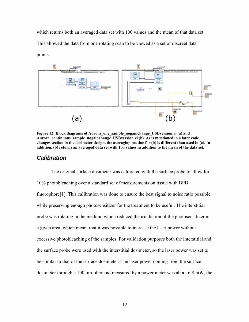
which returns both an averaged data set with 100 values and the mean of that data set.

This allowed the data from one rotating scan to be viewed as a set of discreet data

points.

Figure 12: Block diagrams of Aurora_one_sample_nogainchange_USBversion.vi (a) and Aurora_continuous_sample_nogainchange_USBversion.vi (b). As is mentioned in a later code changes section in the dosimeter design, the averaging routine for (b) is different than used in (a). In addition, (b) returns an averaged data set with 100 values in addition to the mean of the data set.

Calibration

The original surface dosimeter was calibrated with the surface probe to allow for

10% photobleaching over a standard set of measurements on tissue with BPD

fluorophore[1]. This calibration was done to ensure the best signal to noise ratio possible

while preserving enough photosensitizer for the treatment to be useful. The interstitial

probe was rotating in the medium which reduced the irradiation of the photosensitizer in

a given area, which meant that it was possible to increase the laser power without

excessive photobleaching of the samples. For validation purposes both the interstitial and

the surface probe were used with the interstitial dosimeter, so the laser power was set to

be similar to that of the surface dosimeter. The laser power coming from the surface

dosimeter through a 100 μm fiber and measured by a power meter was about 6.8 mW, the

13

laser power from the interstitial dosimeter with the same measurement setup was 7.8

mW.

The calibration procedure for the surface probe was to place the probe on black

foam, take 5 measurements at 4 different gain levels, move the probe to green foam that

happens to fluoresce, and take 5 more measurements at the same 4 gains. The

measurements on the black foam were used to determine the dark noise in the system,

and the measurements on the green foam were used to scale measurements so that each

gain level should produce equivalent fluorescence intensities. During the course of the

experiments, it became clear that the fiber in the interstitial probe fluoresces. As a result,

the calibration procedure was changed to taking a measurement in a dark room, and then

moving the probe to a fluorescent liquid phantom. The dark room measured the dark

noise with the fiber fluorescence, and liquid phantom calibration allowed the scaling

factors to be calculated with the fluorescence accounted for.

The fiber appeared to photobleach as more measurements were taken, but

unfortunately the bleaching was not permanent. After a short period of time the fiber

regained the full fluorescence. This only happened with the interstitial probe and not with

the surface probe; so it was very unlikely that the problem was with the interstitial

dosimeter. This property of the fiber affects some of the measurements taken while

characterizing the probe. The photobleaching is shown in Figure 13.

14

Figure 13: Photobleaching of fluorescence in side firing fiber used in the interstitial probe. These measurements were taken with the interstitial probe in free space in a dark room. With that experimental setup the results without bleaching would be a constant measurement, but in this case a large degree of variability can be seen. The photobleaching effect appeared to be temporary which made calibrating the probe to eliminate the effect of this phenomenon difficult.

New Dosimeter Design

The interstitial dosimeter is based generally on the surface dosimeter (Aurora

Optics Inc., Hanover NH). The interstitial dosimeter retains the same basic layout, has a

similar design, and similar components. The dosimeter uses a laser modulated on and off

at 200 Hz to excite fluorescence in the tissue, and a filter to minimize the excitation light

from the measured signal, a shutter to keep stray light away from the photomultiplier tube

when measurements are not being acquired, and a photomultiplier tube to measure the

fluorescence. The system generally keeps the photomultiplier tube on and charged when

operational, and the input light is simply allowed in by opening the shutter. The laser is

15

modulated with a square wave so that the dark noise signal can be subtracted from the

emission signal during each measurement. This measurement scheme leads to a

differential measurement instead of an absolute measurement, and improves the overall

accuracy of the system. In addition, various methods of reducing noise from the acquired

signal that were implanted in the surface dosimeter were updated for the interstitial

dosimeter. The components in the interstitial dosimeter are updated versions of those

used in the surface dosimeter.

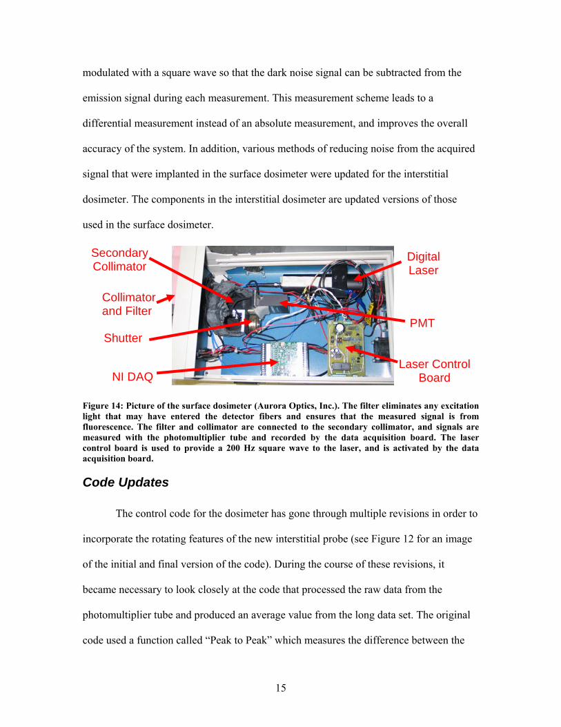
Figure 14: Picture of the surface dosimeter (Aurora Optics, Inc.). The filter eliminates any excitation light that may have entered the detector fibers and ensures that the measured signal is from fluorescence. The filter and collimator are connected to the secondary collimator, and signals are measured with the photomultiplier tube and recorded by the data acquisition board. The laser control board is used to provide a 200 Hz square wave to the laser, and is activated by the data acquisition board.

Code Updates

The control code for the dosimeter has gone through multiple revisions in order to

incorporate the rotating features of the new interstitial probe (see Figure 12 for an image

of the initial and final version of the code). During the course of these revisions, it

became necessary to look closely at the code that processed the raw data from the

photomultiplier tube and produced an average value from the long data set. The original

code used a function called “Peak to Peak” which measures the difference between the

NI DAQ

Digital Laser

Laser Control Board

PMT Shutter

Secondary Collimator

Collimator and Filter

16

maximal peak and the minimal peak. Unfortunately, the signal typically started low and

there was often noise in the measurement.

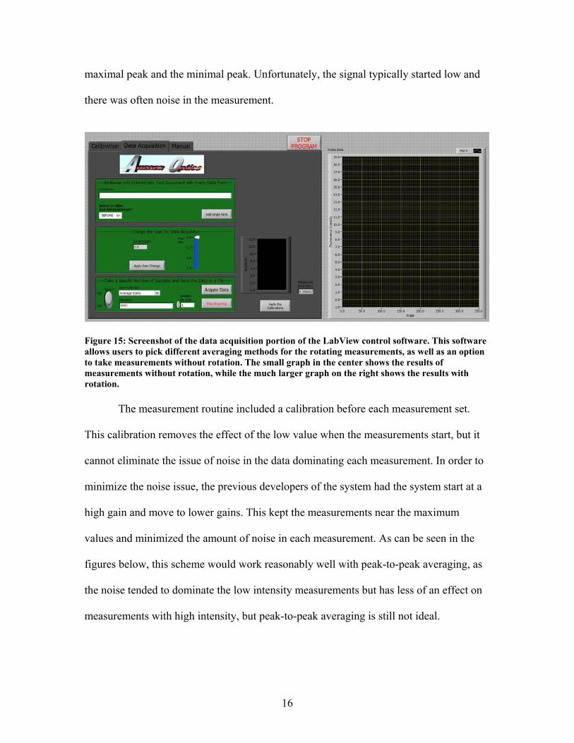
Figure 15: Screenshot of the data acquisition portion of the LabView control software. This software allows users to pick different averaging methods for the rotating measurements, as well as an option to take measurements without rotation. The small graph in the center shows the results of measurements without rotation, while the much larger graph on the right shows the results with rotation. The measurement routine included a calibration before each measurement set.

This calibration removes the effect of the low value when the measurements start, but it

cannot eliminate the issue of noise in the data dominating each measurement. In order to

minimize the noise issue, the previous developers of the system had the system start at a

high gain and move to lower gains. This kept the measurements near the maximum

values and minimized the amount of noise in each measurement. As can be seen in the

figures below, this scheme would work reasonably well with peak-to-peak averaging, as

the noise tended to dominate the low intensity measurements but has less of an effect on

measurements with high intensity, but peak-to-peak averaging is still not ideal.

17

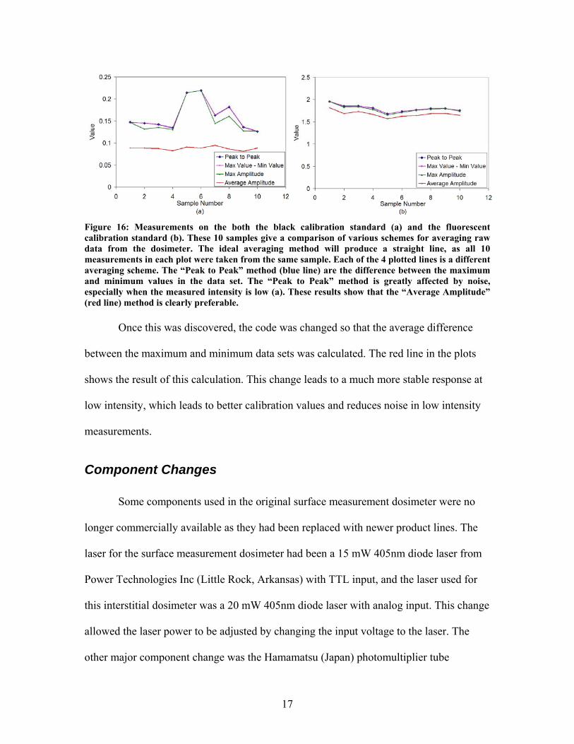
Figure 16: Measurements on the both the black calibration standard (a) and the fluorescent calibration standard (b). These 10 samples give a comparison of various schemes for averaging raw data from the dosimeter. The ideal averaging method will produce a straight line, as all 10 measurements in each plot were taken from the same sample. Each of the 4 plotted lines is a different averaging scheme. The “Peak to Peak” method (blue line) are the difference between the maximum and minimum values in the data set. The “Peak to Peak” method is greatly affected by noise, especially when the measured intensity is low (a). These results show that the “Average Amplitude” (red line) method is clearly preferable. Once this was discovered, the code was changed so that the average difference

between the maximum and minimum data sets was calculated. The red line in the plots

shows the result of this calculation. This change leads to a much more stable response at

low intensity, which leads to better calibration values and reduces noise in low intensity

measurements.

Component Changes

Some components used in the original surface measurement dosimeter were no

longer commercially available as they had been replaced with newer product lines. The

laser for the surface measurement dosimeter had been a 15 mW 405nm diode laser from

Power Technologies Inc (Little Rock, Arkansas) with TTL input, and the laser used for

this interstitial dosimeter was a 20 mW 405nm diode laser with analog input. This change

allowed the laser power to be adjusted by changing the input voltage to the laser. The

other major component change was the Hamamatsu (Japan) photomultiplier tube

18

assembly. The photomultiplier tube in the surface measurement dosimeter had peak

sensitivity near 400 nm, and could provide a gain of approximately 0.6 V/nW at 690 nm.

The photomultiplier tube for the interstitial dosimeter had peak sensitivity closer to 500

nm and could provide a gain of approximately 6.0 V/nW at 690 nm. This adds an order of

magnitude to the detection sensitivity at the wavelength of verteporfin’s fluorescence. In

addition, the wavelength dependence of the sensitivity of the photomultiplier tube in the

newer dosimeter at 690 nm was less than that of the photomultiplier tube in the surface

dosimeter, so dispersion of light in the fibers should not affect the measurements of the

interstitial dosimeter as much as it would affect the measurements of the surface

dosimeter.

Design Changes

The limiting factors of the surface measurement dosimeter were the repeatability

of measurements and the signal to noise ratio at low photosensitizer concentrations.

Changing to the interstitial probe improved the measurement repeatability as coupling

errors were eliminated, but the design of the interstitial probe reduced the signal strength

and the fiber added noise in the form of fluorescence. With the interstitial probe the major

limiting factor of the dosimeter was the signal to noise ratio. The need to improve signal

to noise ratio was the reason for and the focus of the redesign effort.

In the surface measurement dosimeter, a fiber coupled collimator was aligned

with an optical filter with a custom made filter holder. The filter holder was bolted to a

secondary collimation tube that ends with a solenoid driven shutter. The photomultiplier

tube was located directly after the shutter. The secondary collimator, shutter, and

photomultiplier tube are inside of a black cloth bag in order to minimize the amount of

19

stray light that can enter the photomultiplier tube. In this design the secondary collimator

did not serve much function. The secondary collimator is a black tube approximately 10

cm long with a 0.8cm inner diameter. The spot size of the collimated light is 2.2mm and

the full angle divergence is 0.018 degrees (Thorlabs Inc.), which means that the

collimated light will not come anywhere near the tube. The effective area of the

photomultiplier tube is 3.7mm by 13.0mm (Hamamatsu), so the tube would only affect

about 40% of the effective area if it was absorbing non-collimated light. In addition, the

construction of the custom fiber holder does not guarantee the alignment of the collimator

with the filter or with the photomultiplier tube.

Figure 17: Exploded Pro-Engineer rendering of the shutter box with photomultiplier tube and shutter. The shutter box is made up of the gray components. Several important features have been labeled including the shutter, an example of the rebated joints used to prevent stray light from entering the system, the location of the threaded hole for the optical tube, adaptor, and collimator assembly, the photomultiplier tube window, and the photomultiplier tube.

Photomultiplier tube

Shutter

Example of a rebated

joint

Threaded hole for optical tube

Photomultiplier tube window

20

For the interstitial dosimeter a fiber coupled collimator is attached to an optical

tube containing a 600 nm long pass filter with an adaptor. The collimator, adaptor, and

optical tube ensure that the filter is orthogonal to the collimated light for optimal filter

performance. The optical tube is connected to a box that contains the shutter and mounts

for the photomultiplier tube. In order to check the accuracy of the assembly, all of the

components except the photomultiplier tube were assembled and a piece of masking tape

was placed across the opening for the photomultiplier tube’s window. The 690 nm laser

light was sent through a fiber into the assembly, and created a spot on the masking tape in

the center of the window for the photomultiplier tube. This location corresponds to the

center of the effective area of the photomultiplier tube when it is attached to the shutter

box.

All the joints on the box containing the shutter and photomultiplier tube mounts,

including the photomultiplier tube mounts, were rebated and taped with three layers of

black optical tape to prevent stray light from entering the system. Two holes were drilled

and tapped in the box to allow it to be secured to the dosimeter with screws. The optical

tube, adaptor, and collimator were screwed into another hole that was drilled and tapped.

Drilling and tapping was chosen for these joints because the threads prevent stray light

from entering the system.

Validation

Before validation, the laser power output of the two dosimeters was checked with

a power meter. The surface dosimeter transmitted about 6.8 mW and the interstitial

dosimeter transmitted about 7.8 mW, both through a 100 μm fiber.

21

A serial dilution phantom study was used to validate the interstitial dosimeter. A

stock solution of 0.0002% ink and .2% Intralipid was mixed in phosphate buffered saline.

A verteporfin solution was made by adding 0.3105 mL of phosphate buffered saline to

12.42 mg of verteporfin, which is itself 97.5% lipid and 2.5% BPD-MA active molecule

(QLT Inc., Vancouver, BC, Canada). For the first dilution 0.2 mL of the verteporfin

solution was added to 20 mL of the Intralipid and ink stock solution for a concentration

of 10μg/mL of BPD-MA molecule in the saline. For each of the 14 successive

concentrations, 10 mL of the previous dilution was added to 10 mL of stock solution to

provide a dilution by half each time. All solutions containing verteporfin were protected

from light at all times.

The dilutions were measured using the surface dosimeter with the surface probe,

the interstitial dosimeter with the surface probe, and the interstitial dosimeter with the

interstitial probe. Each measurement shown is a single data point averaged over a 1

second acquisition time. Measurements were done in 50 mL clear plastic tubes, with at

least 1 cm of the solution on all sides of the probe. The tubes were kept inside a black box

for the duration of the measurements to minimize the effect of stay light on the

measurements and to protect the samples.

The stock solution was found to be fluorescent, most likely due to the ink used to

add absorption to the solution. The stock solution had an intensity value of 0.097 for the

surface probe with the surface dosimeter, and 0.478 for the surface probe with the

interstitial dosimeter. The interstitial probe also showed the same result. In all cases the

fluorescence of the stock solution was subtracted from the measurements of fluorescence

intensity.

22

Measurements with the surface probe show a linear increase in fluorescence

intensity with increasing concentrations of verteporfin. The noise level of surface

dosimeter was equal to the signal intensity of the lower concentrations of verteporfin in

solution, but that limit was not reached with the interstitial dosimeter. The results show

that the surface dosimeter using the surface probe can detect concentrations of BPD-MA

molecule on the order of 10-5 mg/mL, while the interstitial probe could detect

concentrations at least on the order of 10-6 mg/mL.

Figure 18: Dosimeter sensitivity study done with a mixture of 0.0002% ink, .2% Intralipid and

various concentrations of BPD-MA molecule in phosphate buffered saline solution. The surface

probe had 6 detectors around each source, and seven source and detector clusters. Measurements

were taken with the surface probe attached to both the surface dosimeter and the interstitial

dosimeter, and with the interstitial probe attached to the interstitial dosimeter. The response to

changing concentration of BPD-MA is linear for both dosimeters. The interstitial probe has limited

sensitivity compared to the surface probe, which is likely due to the fluorescence of the fibers in the

interstitial probe.

23

The results for the interstitial dosimeter with the interstitial probe are linear as

well until the concentration of BPD-MA molecule is on the order of 10-4 mg/mL. This

poor sensitivity is likely due to the large degree of observed fluorescence in the side

firing fiber, and could likely be improved by eliminating that source of error.

The changes in design and component choice resulted in the improved sensitivity

of the interstitial dosimeter. The fluorescence intensity measured by the interstitial

dosimeter changes linearly with changing concentrations of BPD-MA molecule. The

interstitial dosimeter with a surface probe is capable of measuring concentrations of

BPD-MA at least on the order of 10-6 mg/mL. Overall, the changes made to the dosimeter

were a success.

Fluorescence Quantum Yield and Oxygen

In some experiments the fluorescence quantum yield of the BPD-MA was found

to be oxygen-sensitive[17]. It is well known that oxygen levels in tumors are not

homogenous[18]. If the oxygen sensitivity is significant at the levels of oxygenation

found in vivo, then it is important to quantify the relationship between oxygen

concentration and fluorescence quantum yield when attempting to calculate drug

concentrations using fluorescence measurements.

The following experiments were completed in an attempt to quantify the

relationship between fluorescence quantum yield and oxygen concentration. The goal of

this set of experiments was to determine whether or not measurements of tissue

oxygenation are necessary for the accurate determination of drug concentrations based on

fluorescence measurements.

24

Methodology

The experiments were all done using verteporfin, which is BPD-MA in liposomal

format with 97.5% lipid and 2.5% BPD-MA by mass. This formulation was obtained

from QLT Inc (Vancouver BC, Canada). The verteporfin mixture was dissolved in di-

methol sulfoxide (DMSO) to make a stock solution at a concentration of 8 mg/mL

verteporfin for an overall concentration of 0.2 mg/mL of BPD-MA molecules in the

DMSO stock solution. These solutions were shielded from direct light at all times, and

kept covered. The powder form was kept at room temperature when not used, and the

liquid solution was used when freshly mixed. Laboratory grade methanol and DMSO

were used in the solutions. Phosphate buffered saline (PBS) solutions were created at

lower concentration by dilution of the stock solution of BPD-MA into PBS. Tissue

phantoms were created in PBS solution with blood, Intralipid and the PBS at 1%

Intralipid and 1% blood.

A chemical microsensor (Diamond General Inc., Ann Arbor MI) was used for

oxygen concentration measurements using a Clarke style electrode in the solution. It was

calibrated using the stock solution at an assumed partial oxygenation of 23% at ambient

conditions. A fully de-oxygenated measurement was obtained by adding yeast to the

stock solution and waiting for the measurement to stabilize near zero. This method was

used to calibrate the measurements to maximum and minimum values of pO2.

An ischemia detector (Spectros Inc., Palo Alto CA) that measures blood oxygen

concentration was used as a secondary oxygenation measurement, using their

commercially available rectal probe. This system measures the reflectance of white light

25

from a small fiber to estimate blood oxygen saturation and blood hemoglobin

concentration measurements.

Fluorescence from verteporfin was measured with the surface dosimeter using the

surface probe. Each measurement from the surface dosimeter was an average of 3

samples, each taken over a period of 250 milliseconds.

Solution samples were shielded from light at all times. After mixing, all solutions

containing verteporfin were wrapped in aluminum foil until they were used. After the

addition of yeast, all solutions were placed in a black box that had the seams taped with

black tape to minimize stray light. The sensors were inserted into the solution through a

hole in this box. The remaining gap between the sensors and the hole was then taped to

minimize stray light.

Results

Published results of the fluorescence quantum yield of BPD-MA are 0.105 in

nitrogen saturated methanol and 0.038 in oxygen saturated methanol. Results published

for BPD-MA in other solutions show similar trends[17]. The methanol experiment was

repeated under the conditions of these previously published results, with the goal of

determining whether liposomal BPD-MA reacts to oxygen in a similar manner.

In a methanol based experiment, 0.1mL of the BPD-MA solution was added to

30mL of methanol. A portion of the mixture was placed into 2 cuvettes. One was bubbled

with ultra high purity nitrogen for 20 minutes, and the other was left in the dark during

that time period. During the bubbling process, a small amount of the mixture was lost so

the level of the liquid in the nitrogen bubble cuvette was slightly lower than that of the

one left open to air. Both samples were then measured with a Flouro-Max 3 (Jobin Yvan

26

Horiba, Edison, New Jersey). The measurements were made with 405 nm light. Both

samples returned similar emission spectra, both with a peak around 690. The nitrogen

bubbled sample had an intensity of about 12.5x106 which was a 4% increase over the

solution that was left open to air which had an intensity of about 12x106.

The results from this experiment did not agree with the published results. One

possible explanation for the lack of increased fluorescence quantum yield in a

deoxygenated environment is that oxygen is still present in the lipids present in the

liposomal formulation of the BPD-MA. If this were the case, it would be possible for the

BPD-MA to excite the oxygen within the lipids instead of releasing a photon in the form

of fluorescence.

To test a situation closer to the in-vivo case, 0.1mL of BPD-MA solution was

added to 30mL of DPBS. About 0.1mL of yeast was added to this mixture at time 0. The

chemical microsensor was used to measure oxygen, and the surface dosimeter was used

to measure fluorescence. The ischemia detector was not used, as it measures the

concentration of oxygenated and deoxygenated blood, and there was no blood in this

solution. Measurements were taken every 30 seconds. The results showed a decrease in

the oxygenation of the solution, likely due to the consumption of oxygen by the yeast in

the solution.

27

Figure 19: Results from the DPBS experiment. Yeast was added to the solution at time zero. De-oxygenation occurred and was measured using the chemical microsensor. The fluorescence was measured using the surface dosimeter. These results show no correlation between measured oxygen levels and fluorescence.

There was no correlation between the oxygen measurement and the fluorescence

measurement. The data did not show the expected increase in fluorescence in the de-

oxygenated solution. The lack of increase in fluorescence can be attributed to a

photobleaching effect as the result of taking the fluorescence measurements. In addition,

there was some noise in the data that would make a 4% increase difficult to see. The

noise in the data can be attributed to heterogeneities in the solution, uneven photo

bleaching, or stray light entering the box that the measurements were taken in.

For the blood, Intralipid, and DPBS experiment, 0.1mL of the BPD-MA solution

was added to 30mL of the stock solution containing blood, DPBS, and Intralipid. At time

0, about 0.25 mL of yeast was added to begin deoxygenating the solution. Measurements

28

were taken every 30 seconds with the chemical microsensor, the ischemia detector, and

the surface dosimeter. In addition, there is some variation in the fluorescence

measurements, but these variations are close to the noise level of the dosimeter, and could

also be caused by heterogeneities in the solution, uneven photo bleaching, or stray light

entering the box that the measurements were taken in.

Figure 20: Results from the blood, Intralipid and PBS experiment. Yeast was added to the solution at time zero. De-oxygenation occurred and was measured using the chemical microsensor and the ischemia detector. The fluorescence was measured using the surface dosimeter. These results show a slope near zero for the fluorescence, indicating no correlation with oxygenation.

29

The fluorescence measurements do not show a huge increase in fluorescence in

the de-oxygenated solution. The fluorimeter results predict a 4% increase in fluorescence,

but this increase is less than the noise seen in this particular measurement. The total

variation in the measurement was around 10%, and most of this is likely due to noise in

the system. This noise could be caused by heterogeneities in the solution, uneven photo

bleaching, or stray light entering the box that the measurements were taken in.

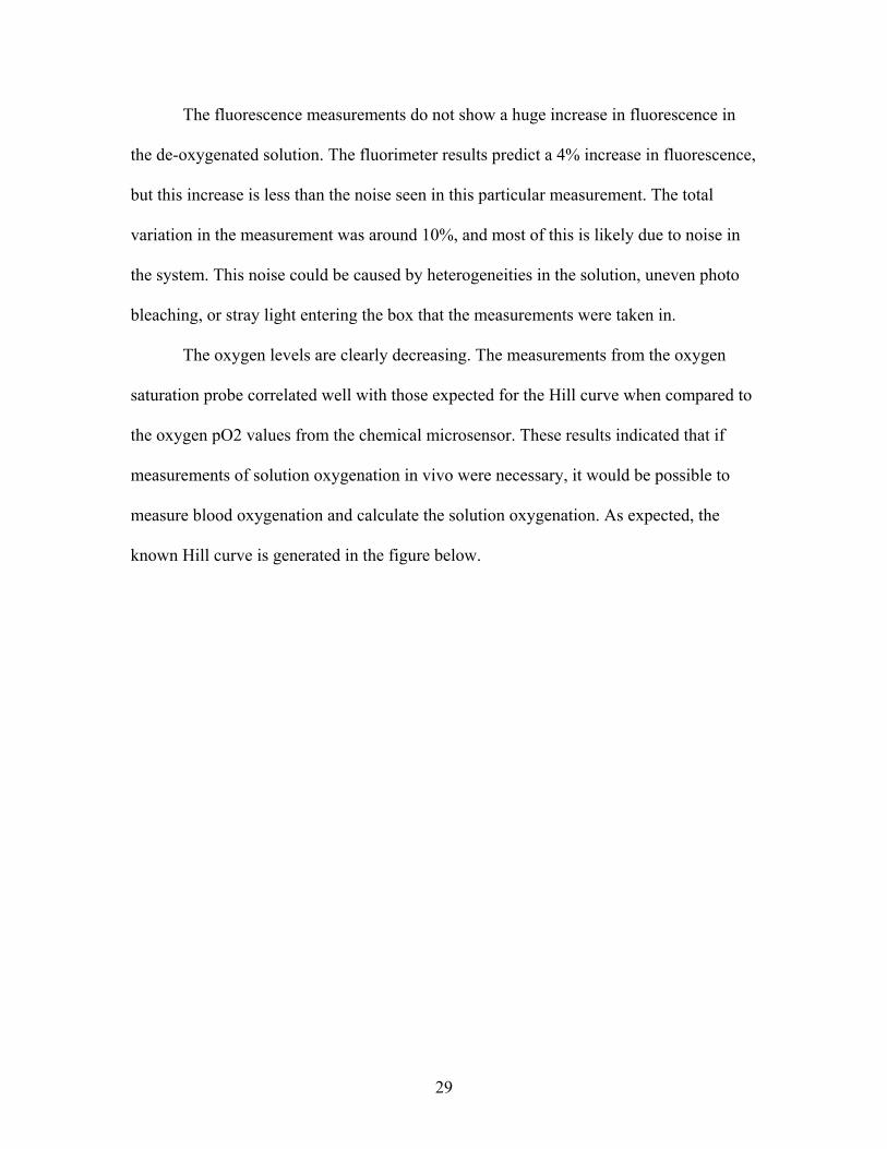
The oxygen levels are clearly decreasing. The measurements from the oxygen

saturation probe correlated well with those expected for the Hill curve when compared to

the oxygen pO2 values from the chemical microsensor. These results indicated that if

measurements of solution oxygenation in vivo were necessary, it would be possible to

measure blood oxygenation and calculate the solution oxygenation. As expected, the

known Hill curve is generated in the figure below.

30

Figure 21: Comparison of the oxygen saturation detector measurement with the oxygenation measurement from the chemical microsensor.

Photobleaching is one possible explanation of why an expected increase in

fluorescence was not seen as the oxygen levels decreased. The amount of yeast added to

the solution was reduced to allow for more measurements and therefore more

photobleaching, but the other variables remained the same.

For the experiment with reduced yeast, 0.1mL of the BPD-MA solution was

added to 30mL of the stock solution containing blood, DPBS, and Intralipid. At time 0,

about .05 mL of yeast was added to begin deoxygenating the solution. Measurements

were taken every 30 seconds with the oxygen sensor, the oxygen saturation detector, and

the fluorescence dosimeter. The results show a decrease in the oxygenation of the

solution, likely due to the consumption of oxygen by the yeast in the solution. Again,

there is variation in the fluorescence measurements. The variation is likely caused by the

31

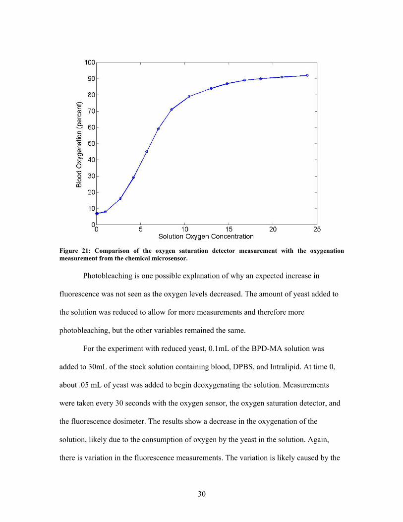
same sources listed above. In this case a monotonic decrease in fluorescence is shown.

Given the results of the case where the oxygen is absorbed more quickly, this phenomena

was likely a result of photobleaching and was not indicative of the correlation between

fluorescence and oxygenation.

Figure 22: Results from the blood, Intralipid and DPBS experiment. Yeast was added to the solution at time zero. De-oxygenation occurred and was measured using the chemical microsensor and the ischemia detector. The fluorescence was measured using the Aurora Dosimeter. A negative slope can be seen in the fluorescence measurements as time increases. This slope can be attributed to the photo bleaching effect. These results explain why a 4% increase in fluorescence was not seen in the previous experiments.

32

Discussion

The results from the methanol experiment did not follow the trend mentioned in

previously published results[17]. The de-oxygenated sample had a 4% increase in

fluorescence compared to the oxygenated sample, while the published results showed a

176% increase in fluorescence. The samples in these experiments did not have oxygen

bubbled as they did in the published case, and it is not clear whether or not the BPD-MA

was in a liposomal format or not in the published results. It is possible that the lipids in

the liposomal BPD-MA retain oxygen, in which case the BPD-MA would not see a de-

oxygenated state in these experiments, but would require more deoxygenation to truly see

the increase. Thus it is possible that the decrease in fluorescence only happens at

extremely high concentrations of oxygen in the solution. However it seems more likely

that the liposomal formulation used here, and used in clinical studies, may be different

from the monomeric formulations used in the Aveline studies.

This trend continues in the experiments done in PBS and in the blood, Intralipid,

and PBS solution. In these cases the increase in fluorescence is not clearly seen. Noise

from heterogeneities in the solution, uneven photo bleaching, or stray light entering the

box that the measurements were taken in may have obscured the increase in fluorescence.

Photobleaching was demonstrated to be significant enough to mask any increase of

fluorescence due to de-oxygenation.

The experiments cover all oxygenation levels typically found in vivo. At these

oxygenation levels, the variation in fluorescence quantum yield of verteporfin is

negligible. The results from all of the experiments show that it is not necessary to

measure the oxygenation of tissues when calculating the concentration of BPD-MA from

33

fluorescence measurements. In all cases the change in fluorescence due to the presence of

oxygen is lower than the noise in the system and photobleaching.

Phantom & Simulation Experiments

Optical property simulation study

To estimate the concentration of photosensitizer based on measured fluorescence

it is necessary to know how much light was available to excite the photosensitizer, and

how much of the fluorescence that was emitted from the photosensitizer made it back to a

detector. Assuming that the distance to the photosensitizer is known, it is necessary to

know the optical properties of the tissue to calculate the attenuation of the light.

The optical properties in tissue are known to be spatially heterogeneous, and they

are difficult to measure in vivo. The optical properties can be expressed in terms of two

main parameters, the absorption coefficient and the scattering coefficient. The absorption

coefficient is represents the amount of light that gets absorbed over a certain distance in a

medium. The scattering coefficient is the amount of light deflected in a medium. The

deflection occurs from objects that are roughly the same size as or smaller than the

wavelength of the light, and as a result the scattering coefficient is wavelength dependent.

The scattering coefficient can be expressed in terms of scattering amplitude and

scattering power as shown below, where a is the scattering amplitude and b is the

scattering power:

'( ) bs aμ λ λ−=

Measurement of optical properties requires multiple measurement points. To

recover both scattering and absorption, two measurements over different distances are

34

required. If both scattering amplitude and scattering power are desired then at least three

separate spectra are required for the measurements. Recovering only the effective

attenuation requires one measurement over some distance[19].

There are two options for measuring attenuation over a given distance in tissue.

The obvious solution is to separate the source and detector by a given distance.

Unfortunately, due to the scattering nature of the light, the distance that any given photon

travels to get from the source to the detector will not be uniform. In this case, the mean

distance that a photon travels will be used for the calculations. The other solution is to

use time gating to measure the photons that take a certain amount of time to reach the

detector. The velocity of the photons is nearly constant, so photons that arrive at the

detector at the same time will have traveled the same distance.

Neither option is practical in the proposed fluorescence dosimeter. The dosimeter

has a single source and detector, and does not have any time gating capability. The

dosimeter is not able to make any measurements of the distance that a photon traveled.

As a result, the optical properties will have to be measured or estimated separately.

If optical properties from a different imaging modality are used then the dosimeter

and that modality will need to be co-registered with each other. There are potential errors

in this co-registration process. The optical properties are time variant, there is the

potential for the organs to have shifted, and the probe location may not be known exactly.

A series of simulations was done to evaluate the potential impact of these inaccuracies in

the knowledge of the optical properties.

These simulations were done using the NIRfast program developed for diffuse

optical tomography. NIRfast uses the diffusion equation, which assumes isotropic

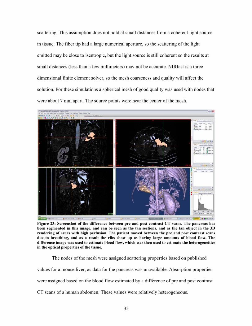
35

scattering. This assumption does not hold at small distances from a coherent light source

in tissue. The fiber tip had a large numerical aperture, so the scattering of the light

emitted may be close to isentropic, but the light source is still coherent so the results at

small distances (less than a few millimeters) may not be accurate. NIRfast is a three

dimensional finite element solver, so the mesh coarseness and quality will affect the

solution. For these simulations a spherical mesh of good quality was used with nodes that

were about 7 mm apart. The source points were near the center of the mesh.

Figure 23: Screenshot of the difference between pre and post contrast CT scans. The pancreas has been segmented in this image, and can be seen as the tan sections, and as the tan object in the 3D rendering of areas with high perfusion. The patient moved between the pre and post contrast scans due to breathing, and as a result the ribs show up as having large amounts of blood flow. The difference image was used to estimate blood flow, which was then used to estimate the heterogeneities in the optical properties of the tissue. The nodes of the mesh were assigned scattering properties based on published

values for a mouse liver, as data for the pancreas was unavailable. Absorption properties

were assigned based on the blood flow estimated by a difference of pre and post contrast

CT scans of a human abdomen. These values were relatively heterogeneous.

36

Figure 24: Screenshot of mesh superimposed over the difference of pre and post contrast CT scans. The difference of the scans was used to estimate blood volume, and that estimate was used to calculate the heterogeneities in optical properties. These properties were assigned to the nodes of the mesh, and were used in the forward finite element simulations shown below. Three different locations were chosen for the light sources. One was the center of

the pancreas. The other two were located next to the artery that wraps around the

pancreas. These locations were chosen because pancreatic cancer often involves this

artery, and the amount of blood in the artery leads to a higher absorption coefficient in

this region.

The first simulation examined the error introduced when the tissue is assumed to

be homogeneous. As can be seen in Figure 25, the error at small distances can be quite

significant, as high as 2 orders of magnitude at one centimeter away if the entire region is

considered homogenous and if the source is near the edge of the pancreas. If the light

source is within the pancreas, the errors are more reasonable.

37

Figure 25: Plot of difference between fluence calculated from heterogeneous optical properties and a prediction using a homogeneous assumption. The simulations were done with a finite element method forward simulation using optical properties calculated from estimated blood concentrations. Three source locations were chosen, one near the center of the pancreas and two close to an artery. The samples near the artery are in different locations, so the results should be different. The difference in the homogeneous results and the heterogeneous results at each node were calculated. This results in multiple differences at each distance so error bars were used to show the standard deviation of this difference. These results are part of a simulation study to determine which assumptions can be made about optical properties in vivo. The first simulation assumes that the source location can be known exactly, and

that the optical properties will remain unchanged between when they are measured and

when the dosimetery measurements are taken. The second and third simulations look at

the effect of errors in locating the light source in the tissue.

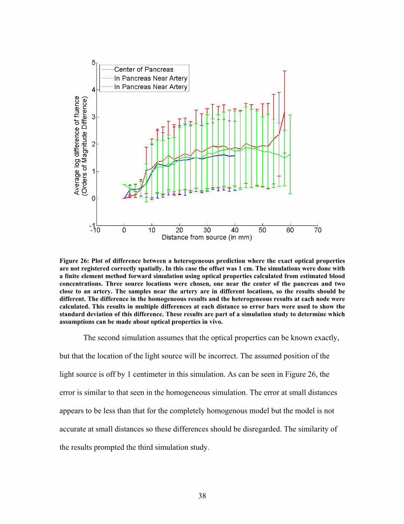
38

Figure 26: Plot of difference between a heterogeneous prediction where the exact optical properties are not registered correctly spatially. In this case the offset was 1 cm. The simulations were done with a finite element method forward simulation using optical properties calculated from estimated blood concentrations. Three source locations were chosen, one near the center of the pancreas and two close to an artery. The samples near the artery are in different locations, so the results should be different. The difference in the homogeneous results and the heterogeneous results at each node were calculated. This results in multiple differences at each distance so error bars were used to show the standard deviation of this difference. These results are part of a simulation study to determine which assumptions can be made about optical properties in vivo. The second simulation assumes that the optical properties can be known exactly,

but that the location of the light source will be incorrect. The assumed position of the

light source is off by 1 centimeter in this simulation. As can be seen in Figure 26, the

error is similar to that seen in the homogeneous simulation. The error at small distances

appears to be less than that for the completely homogenous model but the model is not

accurate at small distances so these differences should be disregarded. The similarity of

the results prompted the third simulation study.

39

Figure 27: This plot shows the difference between a homogeneous prediction where the optical properties are not registered correctly and a heterogeneous model. In this case the offset was 1 cm. The simulations were done with a finite element method forward simulation using optical properties calculated from estimated blood concentrations. Three source locations were chosen, one near the center of the pancreas and two close to an artery. The samples near the artery are in different locations, so the results should be different. The difference in the homogeneous results and the heterogeneous results at each node were calculated. This results in multiple differences at each distance so error bars were used to show the standard deviation of this difference. These results are part of a simulation study to determine which assumptions can be made about optical properties in vivo. The results of this graph show that there is a large difference between the prediction and the actual fluence, but that it is similar to that of the heterogeneous prediction with the same coregistration error. These results indicated that there is no advantage to using heterogeneous optical properties if there were coregistration errors. The third simulation study assumed that the homogeneous model was used with

inaccuracies in the placement of the light source. This simulation shows similar results to

the second simulation, with slightly better results at 1 centimeter. The error of the second

simulation appears to grow slowly and level out, while there is a steady increase in error

as the distance increases with the third simulation.

40

These simulations indicate that inaccurate optical properties will cause significant

error in the estimation of light fluence in tissue. If accurate knowledge of the light fluence

is desired then accurate maps of the optical properties will be required. In addition, any

error in coregistering the maps of the optical properties with the location of the source

will result in significant errors.

From these simulations it is clear that without an accurate method of measuring

the optical properties at the time of the dosimetery the results will be inaccurate. When

measurements are taken before the dosimetery peristaltic motion will generate

inaccuracies in the spatial relationship between the optical properties, the blood volume

in the tissue may change, and the organ may shift. Figure 27 and Figure 26 show that

when the spatial information is not correct assuming homogeneous optical properties

does not induce additional error. Assuming homogeneous optical properties may even be

more accurate than assuming heterogeneous optical properties in some cases.

Phantom Studies

The performance of the surface probe has been well characterized in previous

experiments, and it has been shown that the geometry of the probe improves its

performance. The following experiments characterize the interstitial probe in a similar

manner, giving quantitative measurements of the sensitivity of the probe at various

distances and qualitative measurements of the probe’s ability to determine the origin of

fluorescence at various distances. Liquid phantom studies were used for this

characterization.

The liquid phantom contained 2 mL of 20% Intralipid and 2 mL of porcine blood

with heparin added to prevent coagulation in 200 mL of phosphate buffered saline. A

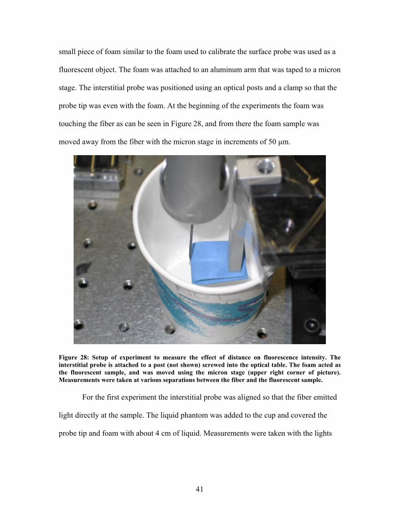
41

small piece of foam similar to the foam used to calibrate the surface probe was used as a

fluorescent object. The foam was attached to an aluminum arm that was taped to a micron

stage. The interstitial probe was positioned using an optical posts and a clamp so that the

probe tip was even with the foam. At the beginning of the experiments the foam was

touching the fiber as can be seen in Figure 28, and from there the foam sample was

moved away from the fiber with the micron stage in increments of 50 μm.

Figure 28: Setup of experiment to measure the effect of distance on fluorescence intensity. The interstitial probe is attached to a post (not shown) screwed into the optical table. The foam acted as the fluorescent sample, and was moved using the micron stage (upper right corner of picture). Measurements were taken at various separations between the fiber and the fluorescent sample.

For the first experiment the interstitial probe was aligned so that the fiber emitted

light directly at the sample. The liquid phantom was added to the cup and covered the

probe tip and foam with about 4 cm of liquid. Measurements were taken with the lights

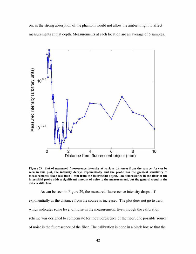
42

on, as the strong absorption of the phantom would not allow the ambient light to affect

measurements at that depth. Measurements at each location are an average of 6 samples.

Figure 29: Plot of measured fluorescence intensity at various distances from the source. As can be seen in this plot, the intensity decays exponentially and the probe has the greatest sensitivity to measurements taken less than 1 mm from the fluorescent object. The fluorescence in the fiber of the interstitial probe adds a significant amount of noise to the measurement, but the general trend in the data is still clear. As can be seen in Figure 29, the measured fluorescence intensity drops off

exponentially as the distance from the source is increased. The plot does not go to zero,

which indicates some level of noise in the measurement. Even though the calibration

scheme was designed to compensate for the fluorescence of the fiber, one possible source

of noise is the fluorescence of the fiber. The calibration is done in a black box so that the

43

fluorescence exiting the side of the fiber cannot enter the fiber again. Fluorescence from

the fiber could be entering the liquid phantom, scattering, and then entering the fiber

again. Fluorescence entering the fiber in this manner would not be accounted for by the

calibration. The intensity of the fluorescence in the fiber was significant compared to the

fluorescence of the foam in the phantom, which added to the problems with noise.

Figure 30: Setup of experiment to measure the effect of distance on detection of the origin of fluorescence. The interstitial probe is attached to a post (not shown) screwed into the optical table. The foam acts as the fluorescent sample, and is moved using the micron stage (upper right corner of picture). Measurements were taken while the fiber rotated at various separations between the fiber and the fluorescent sample. This picture was taken with the 0.2% Intralipid and 1% blood phantom being added to the cup.

For the second experiment the interstitial probe was aligned so that the fiber

emitted light directly opposite the sample. The sample was modified to present a smaller

cross section so that it determining the direction of the fluorescence would be easier. The

44

liquid phantom was added to the cup and covered the probe tip and foam with about 4 cm

of liquid. Measurements were taken with the lights on, as the strong absorption of the

phantom would not allow the ambient light to affect measurements at that depth. Each

measurement was taken as the probe rotated through 360 degrees, and the data displayed

is an average of many measurements.

Figure 31: Plot of the intensity at different rotation angles over distance for the interstitial probe. The fluorescent object was located at 180 degrees. These results with 1% Intralipid and 1% blood show that the probe cannot detect the direction of fluorescence when optical properties are similar to those found in vivo. Also clear from this plot is that most of the sensitivity to in the measurement is at distances less than 1 mm.

The results in Figure 31 and Figure 32 show that the fluorescence is relatively

uniform in all directions. This result is not surprising, as the liquid phantom is a highly

scattering model and the acceptance angle study showed that the side firing fiber has a

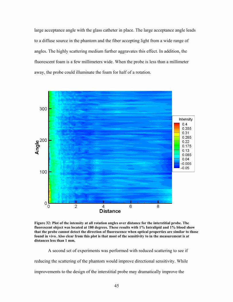
45

large acceptance angle with the glass catheter in place. The large acceptance angle leads

to a diffuse source in the phantom and the fiber accepting light from a wide range of

angles. The highly scattering medium further aggravates this effect. In addition, the

fluorescent foam is a few millimeters wide. When the probe is less than a millimeter

away, the probe could illuminate the foam for half of a rotation.

Figure 32: Plot of the intensity at all rotation angles over distance for the interstitial probe. The fluorescent object was located at 180 degrees. These results with 1% Intralipid and 1% blood show that the probe cannot detect the direction of fluorescence when optical properties are similar to those found in vivo. Also clear from this plot is that most of the sensitivity to in the measurement is at distances less than 1 mm. A second set of experiments was performed with reduced scattering to see if

reducing the scattering of the phantom would improve directional sensitivity. While

improvements to the design of the interstitial probe may dramatically improve the

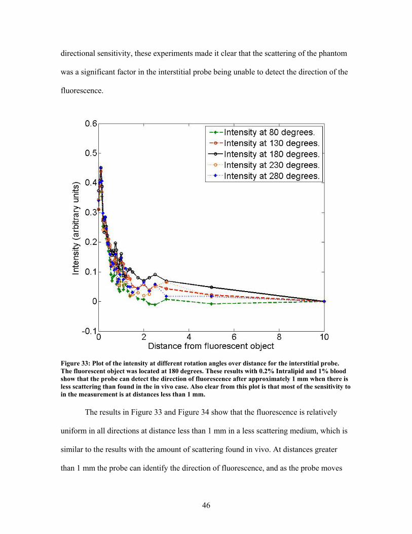
46

directional sensitivity, these experiments made it clear that the scattering of the phantom

was a significant factor in the interstitial probe being unable to detect the direction of the

fluorescence.

Figure 33: Plot of the intensity at different rotation angles over distance for the interstitial probe. The fluorescent object was located at 180 degrees. These results with 0.2% Intralipid and 1% blood show that the probe can detect the direction of fluorescence after approximately 1 mm when there is less scattering than found in the in vivo case. Also clear from this plot is that most of the sensitivity to in the measurement is at distances less than 1 mm. The results in Figure 33 and Figure 34 show that the fluorescence is relatively

uniform in all directions at distance less than 1 mm in a less scattering medium, which is

similar to the results with the amount of scattering found in vivo. At distances greater

than 1 mm the probe can identify the direction of fluorescence, and as the probe moves

47

further away this results get better. Unfortunately, the sensitivity of the probe is far

greater at distances less than 1 mm, and there is more scattering in vivo than there was in

this set of experiments.

Figure 34: Plot of the intensity at all rotation angles over distance for the interstitial probe. The fluorescent object was located at 180 degrees. These results with 0.2% Intralipid and 1% blood show that the probe can detect the direction of fluorescence after approximately 1 mm when there is less scattering than found in the in vivo case. Also clear from this plot is that most of the sensitivity to in the measurement is at distances less than 1 mm. During the course of the directional sensitivity measurements the liquid phantom

stratified. This led to erroneous measurements. The last measurement was taken at 10

mm, and this measurement was subtracted from the other measurements as a way to

eliminate this systemic noise from the measurements. The stratification occurred

gradually, so the earlier measurements had not been affected as much as the later

48

measurements. In addition the fluorescence of the fiber had a gradual bleaching as can be

seen in Figure 13. These time dependences lead to the discrepancies seen at 0 degrees and

360 degrees in Figure 34.

Mouse Experiments

A series of mouse experiments were performed as a part of a study in pancreatic

cancer models. The experiments used the surface dosimeter with the surface probe and

the interstitial probe to measure the pharmacokinetics of verteporfin in tumors and in

normal tissues in mice.

AsPC1 Pharmacokinetics Measured with the Surface Probe

A sample of the AsPC1 tumor line was obtained from Massachusetts General

Hospital collaborators and the cells grown up in tissue culture by Kim Samkoe at

Dartmouth. Up to 1 million cells were used for injection, with the cells suspended in

Matrigel. These were injected into 4 SCID mice subcutaneously in the right hind leg and

into 10 SCID mice orthotopically. These incubated for approximately 21-28 days until

the tumors were at least 6mm in all directions, at which point the measurements were

taken, the mice were sacrificed, and sections were removed for histological staining.

49

Figure 35: Subcutaneous AsPC1 tumor (a) and orthotopic AsPC1 tumor (b). These images were taken by Venkataramanan Krishnaswamy (a) and Kim Samkoe (b). The tumors were allowed to grow until they measured approximately 6mm, as assessed with calipers for the subcutaneous model and measured with 3T MR system for the orthotopic model. The mice with the subcutaneous tumors were free fed and provided with a

continuous supply of water. The mice with orthotopic tumors were fasted before the

measurements to minimize the effect of the fluorescence from the food on the

measurements. For all mice the experimental procedure was to anesthetize with a

Ketamine/Xylazine mixture, open the skin around the tumor, take pre-injection

measurements, inject verteporfin at a concentration of 1mg/kg of the BPD-MA active

molecule, take post-injection measurements, sacrifice the mouse, and take histological

samples. The verteporfin was mixed in phosphate buffered solution with magnesium and

calcium. Two of the mice with subcutaneous tumors and two of the mice with orthotopic

tumors died before the measurements could be completed. In two of the cases a bad

reaction to anesthesia led to death, one mouse died during the injection procedure, and

one mouse was killed by one of the other mice in its cage.

50

All measurements were taken with the surface dosimeter. Measurements were

taken with the surface probe for 2 mice with subcutaneous tumors and for 8 mice with

orthotopic tumors. Measurements were taken on tumor tissue and on normal tissue both

before and after injection. The measurements before injection and on normal tissue

served as a reference point for the tumor measurements. The surface probe was placed on

the tumor site, then on the normal site manually. The same measurement sites were

targeted, but repeatability was low and coupling errors were present. Each data point is an

average of 3 separate measurements. At least 3 measurements were taken before the

injection. After injection measurements were taken every minute for both the tumor and

normal tissues. The normal tissue for the subcutaneous tumor was the muscle tissue near

the tumor site. The normal tissue for the orthotopic tumor was the liver, which was

chosen for the rapid uptake of and relatively high accumulation of photosensitizer.

Injections were given in the tail vein for all animals. In the first animal, the tail

had been damaged by other mice in the cage, so half of the injection was given intra-

peritoneal. This affected results as can be seen in plot (a) of Figure 36.

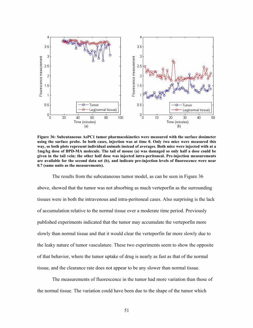
51

Figure 36: Subcutaneous AsPC1 tumor pharmacokinetics were measured with the surface dosimeter using the surface probe. In both cases, injection was at time 0. Only two mice were measured this way, so both plots represent individual animals instead of averages. Both mice were injected with at a 1mg/kg dose of BPD-MA molecule. The tail of mouse (a) was damaged so only half a dose could be given in the tail vein; the other half dose was injected intra-peritoneal. Pre-injection measurements are available for the second data set (b), and indicate pre-injection levels of fluorescence were near 0.7 (same units as the measurements). The results from the subcutaneous tumor model, as can be seen in Figure 36

above, showed that the tumor was not absorbing as much verteporfin as the surrounding

tissues were in both the intravenous and intra-peritoneal cases. Also surprising is the lack

of accumulation relative to the normal tissue over a moderate time period. Previously

published experiments indicated that the tumor may accumulate the verteporfin more

slowly than normal tissue and that it would clear the verteporfin far more slowly due to

the leaky nature of tumor vasculature. These two experiments seem to show the opposite

of that behavior, where the tumor uptake of drug is nearly as fast as that of the normal

tissue, and the clearance rate does not appear to be any slower than normal tissue.

The measurements of fluorescence in the tumor had more variation than those of

the normal tissue. The variation could have been due to the shape of the tumor which

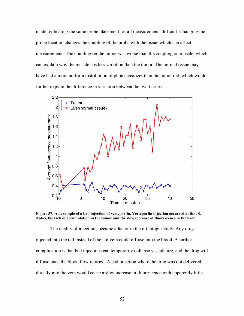
52

made replicating the same probe placement for all measurements difficult. Changing the

probe location changes the coupling of the probe with the tissue which can affect

measurements. The coupling on the tumor was worse than the coupling on muscle, which

can explain why the muscle has less variation than the tumor. The normal tissue may

have had a more uniform distribution of photosensitizer than the tumor did, which would

further explain the difference in variation between the two tissues.

Figure 37: An example of a bad injection of verteporfin. Verteporfin injection occurred at time 0. Notice the lack of accumulation in the tumor and the slow increase of fluorescence in the liver. The quality of injections became a factor in the orthotopic study. Any drug

injected into the tail instead of the tail vein could diffuse into the blood. A further

complication is that bad injections can temporarily collapse vasculature, and the drug will

diffuse once the blood flow returns. A bad injection where the drug was not delivered

directly into the vein would cause a slow increase in fluorescence with apparently little

53

accumulation in the tumor, for some unknown reason. An example of this is shown in

Figure 37. So these bad injections were excluded from the orthotopic study.

Figure 38: Mean of the normalized results from the orthotopic AsPC1 tumor study (n=4 animals). Verteporfin injection occurred at time 0, and only good injection animals were used in this analysis. Each data set was normalized so the maximum measurement before averaging was set to one. The error bars shown are the standard deviation between animals, which is why the measurements are below 1. This was done to prevent variations in the concentration of the drug from altering the results in an averaged study. See Figure 37 for an example of a bad injection. Measurements were taken when the tumors were approximately 6 mm in size. The results from the orthotopic study show a rapid uptake of photosensitizer in

both the tumor and normal tissues. The liver shows far more fluorescence than the tumor,

and the fluorescence increases with time. The liver is an organ with high blood flow that

filters the blood, so the accumulation of drugs in the liver was expected. The fluorescence

of the orthotopic tumors indicates a moderately heterogeneous distribution, but the

average fluorescence of each animal relative to the fluorescence of the liver was stable.

The error bars in the plots show that the fluorescence in the liver varied far more from

54

animal to animal than the fluorescence of the tumor. The level of variability in the liver

compared to the tumor was a surprise, as photosensitizer concentrations were expected to

be highly heterogeneous, with increasing heterogeneity as time increased.

The fluorescence orthotopic tumor appears to be less heterogeneous than the

subcutaneous model. This difference could be due to different vasculature in the

subcutaneous and orthotopic models. Published research has shown that growing tumors

in different parts of the body changes the tumor structure. This would explain a variation

in photosensitizer heterogeneity that would lead to differences in fluorescence

heterogeneity. Another factor in this phenomenon is the thickness of the mouse liver. The

liver is thicker in the center of the organ, and gets thinner towards the edges. If the probe

was placed closer to the edge, it is possible that the organs below the liver would be

included in the measurement. In this case, slight variations in probe placement could

cause large variations in measured fluorescence.

AsPC1 Pharmacokinetics Measured with the Interstitial Probe

The AsPC1 tumors were grown as described above for this experiment, and

grown to similar size at which point the measurements were taken, the mouse were

sacrificed, and sections were removed for histological staining. As before mice were free

fed and provided with a continuous supply of water. The experimental procedure was to

anesthetize with a Ketamine/Xylazine mixture, take pre-injection measurements, inject

verteporfin at a concentration of 1mg/kg of the BPD-MA active molecule, take post-

injection measurements, sacrifice, and take histological samples. The verteporfin was

mixed in phosphate buffered solution with magnesium and calcium.

55

Measurements were taken with the interstitial probe using the surface dosimeter.

The probe was inserted with the fiber retracted inside the needle. The exact location of

the needle tip was unknown, but it was placed near the center of the tumor. Once the

needle tip was near the center, the needle was pulled back to expose the fiber tip to the

tissue. The fiber had been a short distance behind the needle tip, so the exact location of

the fiber in the tissue was unknown. Once the measurements had been completed, the

fiber was retracted into the needle and the needle was then removed from the tissue. After

the measurements the fiber tip was examined and found to be intact.

Measurements were taken at all angles every minute after injection. The probe

remained in one location for the entire set of measurements which eliminated error due to

coupling differences between measurements. Unfortunately, reference measurements of

normal tissue were unavailable because the probe was always in the tumor tissue.

56

Figure 39: Pharmacokinetics of verteporfin injected into a subcutaneous AsPC1 tumor grown on the right hind leg of a SCID mouse measured with the interstitial probe with the surface dosimeter. Verteporfin injection occurred at time 0, and measurements were taken every minute after injection. Measurements were taken at all angles. A relatively homogeneous fluorescence measurement was observed, with two fluorescence peaks at 35 and 85 minutes.

The interstitial measurements of the subcutaneous tumor with the interstitial probe

shows relatively homogeneous levels of fluorescence compared to the corresponding

measurements with the surface probe. This can be explained by the lack of coupling

errors in the interstitial probe, and by the sensitivity close to the probe tip and the

directional accuracy quite far from the probe tip as seen in Figure 29 and Figure 34.

These profiles make it difficult for the probe to detect the direction of fluorescence in

vivo, which would made measurements taken in vivo look far more homogeneous than

they may actually be.

57

The interstitial measurements of the subcutaneous tumor show a slowed increase

in fluorescence with a peak at 35 minutes, and a much larger secondary peak at 85

minutes. This pattern was not expected, as it is unusual for the concentration of

photosensitizer to accumulate, clear, and then begin to accumulate again. The only way

that those pharmacokinetics could be created is if a large amount of photosensitizer had

been injected into the tail instead of the tail vein and it began to perfuse into the blood

stream after an hour had passed. The other possibility is that the probe tip was located in

a region with a very slow perfusion rate near a vessel. In this case, the first fluorescence

peak could be the vessel, which would appear to be a uniform fluorescence if it were less

than a millimeter away, and the second peak would be the photosensitizer perfusing

towards the probe tip. In any case, this individual data point should not be over

interpreted.

Panc1 Pharmacokinetics Measured with the Surface Probe

A sample of the Panc-1 tumor line was obtained from the Massachusetts General

Hospital collaborators and the cells grown up in tissue culture by Kim Samkoe. The

Panc1 tumors were injected into 10 SCID mice orthotopically in Matrigel. The tumors

were allowed to grow until they measured at least 6mm in all directions, at which point

the measurements were taken, the mice were sacrificed, and sections were removed for

histological staining.

The mice with the subcutaneous tumors were free fed and provided with a

continuous supply of water. The mice were fasted before the measurements to minimize

the effect of the fluorescence from the food on the measurements. For all mice the

experimental procedure was to anesthetize with a Ketamine/Xylazine mixture, resect the

58

skin around the tumor, take pre-injection measurements, inject verteporfin at a

concentration of 1mg/kg of the BPD-MA active molecule, take post-injection

measurements, sacrifice the mouse, and take histological samples. The verteporfin was

mixed in phosphate buffered solution with magnesium and calcium.

All measurements were taken with the surface dosimeter. Measurements were

taken with the surface probe for all mice on tumor tissue and on normal tissue both before

and after injection. The measurements before injection and on normal tissue served as a

reference point for the tumor measurements. The surface probe was placed on the tumor

site, then on the normal site manually. The same measurement sites were targeted, but

repeatability was low and coupling errors were present. Each data point is an average of 3

separate measurements. At least 3 measurements were taken before the injection. After

injection measurements were taken every minute for both the tumor and normal tissues.

The normal tissue for this study was the liver, which was chosen for the rapid uptake of

and relatively high accumulation of photosensitizer.

Injections were given in the tail vein for all animals. Injections where the vein

was missed and the injection was into the tail were discounted from the study for reasons

discussed in the AsPC1 studies. The results shown below are the normalized averages of

the remaining mice.

59

Figure 40: Mean of the normalized results from the orthotopic Panc1 tumor study (n=4 animals). Verteporfin injection occurred at time 0. Each data set was normalized so the maximum measurement before averaging was set to one. The error bars shown are the standard deviation between animals, which is why the measurements are below 1. This was done to prevent variations in the concentration of the drug from altering the results in an averaged study. It appears that the fluorescence increase begins before time 0, part of this effect is that measurements are not taken while the drug is injected so the last pre-injection measurement can be some time before the first post injection measurement. The injection times were recorded to the minute, so there may be nearly a full minute of error from the lack of precision in that measurement. Measurements were taken when the tumors were approximately 6 mm in size. The results from the study show a rapid uptake of photosensitizer in both the

tumor and normal tissues. The liver shows far more fluorescence than the tumor, and the

fluorescence increases with time. As discussed in the AsPC1 study, the accumulation of

drugs in the liver is expected. The fluorescence of the orthotopic tumors indicates a

moderately heterogeneous distribution, and the average fluorescence relative to the

fluorescence of the liver reflects this. The error bars in the plots show that the

fluorescence in the liver varied far more than that of the tumor. The level of variability in

60

the liver compared to the tumor was similar to the level of variability found in the AsPC1

studies, which is likely due to the thickness of the liver and the potential for sampling

tissues beneath the liver, coupling errors, and heterogeneity in photosensitizer

concentrations in the liver.

The level of fluorescence in the tumor relative to the fluorescence in the liver in

the Panc1 study was similar to that of the AsPC1 study. The Panc1 tumors appeared to

have more heterogeneous fluorescence distributions than the AsPC1 tumors did. Overall,

the verteporfin had similar pharmacokinetics in both pancreatic tumor models.

Conclusions

In this work an interstitial dosimeter, based generally on an existing surface

dosimeter was designed and built, and novel rotating probe design built and evaluated.

The redesigned dosimeter for interstitial use was more than 4 times more sensitive than

the existing dosimeter for surface measurements due to design improvements. The

effective measurement depth of the interstitial probe is limited to a few hundred microns,

and the probe cannot determine the direction of the fluorescence in a medium with optical

properties similar to those found in vivo.

The fiber optic portion of the interstitial probe was the limiting factor of the

device. The fiber fluoresced significantly, and the fluorescence changed with respect to

time. The current hypothesis is that the sheathing of the fiber is fluorescent, and that laser

light is entering the sheathing due to a combination of transmission modes in the cladding

and mismatched cladding sizes between fibers in the system. In addition, the geometry of

the side firing fiber led to a source and detector with a large numeric aperture, which

61

made detection of fluorescence direction difficult. A different fiber design could greatly

improve the performance of the probe.

The code updates done during the course of this research improved the

performance of both the interstitial dosimeter and the surface dosimeter. The change to

the averaging code improved the calibration of the systems as well as reducing

measurement noise for low fluorescence measurements. These improvements reduced the

effect of changing gains during measurements and reduce variation between

measurements.

Experiments that characterized the effect of oxygen fluorescence quantum yield

covered all oxygenation levels typically found in vivo showed that at these oxygenation

levels the variation in fluorescence quantum yield of verteporfin is negligible. Therefore,

it is not necessary to measure the oxygenation of tissues when calculating the

concentration of BPD-MA from in vivo fluorescence measurements. In all cases the

change in fluorescence due to the presence of oxygen at the levels found in vivo was

lower than the noise in the system and photobleaching. This factor is important to know

as if oxygenation changes did affect the fluorescence, as was originally believed, then

this would make the data from the dosimeter less reliable in its current form. However

now we have greater confidence in that we can interpret the data quantitatively in terms

of being linear with concentration.

Simulation studies showed that assuming homogeneous optical properties for

when the optical properties were heterogeneous would introduce significant errors in

fluence calculations. Further simulations showed that homogeneous optical properties

were just as accurate as heterogeneous optical properties when there were moderate co-

62

registration errors. Co-registration errors could be induced from organ motion and

discrepancies between the assumed probe position and the actual probe position. Co-

registration errors were assumed to be likely, so the homogeneous assumption was used.

Positioning errors and coupling errors are the primary source of error in the

measurements taken with the surface probe. If there were a way to make the coupling

more uniform and more repeatable, the precision of the surface measurements would

increase dramatically. The measurements taken with the surface probe are still useful and

can reveal trends in data in vivo. The interstitial probe did not add much information to in

vivo data due to the sensitivity limits. As was mentioned above, a redesign of the

interstitial probe could solve some of these issues.

Overall, this project has had intermediate successes in a few different aspects of

dosimetry. The dosimeter design has been improved and a novel probe has been

designed, evaluated, and characterized. The assumptions necessary for pretreatment

dosimetry have been evaluated, and were found to be reasonable. Establishment and

study of the AsPC-1 and Panc-1 tumor lines were completed and the uptake of the drug

relative to the liver has been quantified.

Future Directions

There are a few design changes that would improve the interstitial dosimeter. The

laser control board for the dosimeter should be redesigned or eliminated if development

of the system continues. The control board design has features which could be improved,

such as providing more convenient connection locations for external contacts. The

current design uses a zener diode and resistor scheme instead of the more stable and

efficient DC/DC converters. If an analog laser is used for future devices, the analog input

63

of the laser could be wired through an illuminated switch to the DAQ board. This

configuration would maintain the safety cutoff for the laser, and would eliminate the need

for a laser control board.

If experiments with a rotating interstitial probe continue, the side firing fiber

should be replaced with a prism or mirror at the end of a traditional fiber. This

arrangement will have a smaller numerical aperture than the side firing fiber, and should

improve the directional sensitivity of the probe. The mechanical design of the probe

could be revised so that it is more compact and much lighter. The large gears currently

used could be replaced with a small gearhead mounted to the motor. Much smaller gears

or a belt system could be used to couple the stepper motor and gearhead to the rotary

joint.

Point measurements of fluorescence values in vivo are possible, and the accuracy

of those measurements has improved over the course of this research. If measurements in

a tissue volume are necessary then multimodal methods for determining the

photosensitizer concentrations in tissue volumes should be considered. It may be possible

to take measurements of photosensitizer concentrations at a few carefully chosen points

and reconstruct for the distribution over the volume using information about blood

perfusion or other biological information from another modality. Given sufficient

computing power, another option would be to use diffuse optical tomography with spatial

information from another modality to reconstruct an optical property map and

photosensitizer concentrations in a tissue volume simultaneously.

Real time treatment dosimetry for photodynamic therapy should be researched

further. A normalized fluorescence signal could be obtained from the treatment fiber by

64

using a dichroic mirror to separate the fluorescence signal from the excitation

wavelength. Another possibility would be to insert a separate detection fiber near the

treatment fiber. In either case, fluorescence measurements could be made continuously

and this dynamic information could be used to characterize the photosensitizer

distribution during treatment in real time. This would allow the treatment to be controlled

dynamically and specific singlet oxygen doses for the tissue could be targeted. In any

case, most of the published data, and the data in this thesis indicates that individual

animals have variability which is not always predictable, and to make photodynamic

therapy more uniform between individuals, pre-treatment or online measurement of

photosensitizer should become more routinely used. The developments in this thesis

have hopefully helped to add some information to this particular area of research.

65

Appendix

Dosimeter LabView Code

The control code for the dosimeters is a relatively large LabView program. The

program has two main components, the calibration routine, and the measurement routine.

The only change to the calibration routine was the switch from the original

“Aurora_one_sample_nogainchange_USBverion.vi” function to the modified version for

the interstitial dosimeter “Aurora_continuous_sample_nogainchange_USBversion.vi” for

reasons explained in the code updates section.

Figure 41: Screenshot of the LabView calibration routine as seen by the user. The background and fluorescence reference buttons are the two buttons in the lower left hand corner of the image. The red oval in the bottom center of the image indicates that the calibration is not complete, once the calibration has been completed the oval will turn green and allow the user to enter the measurement screen. In the upper center is a button to load previous calibrations. The calibration code works as follows: User Clicks on Black Reference

1) User prompted to place probe on black foam 2) Measurements are taken at a gain of 0.8

3) Measurements are averaged and stored in a “Background” vector 4) Gain is lowered

5) System waits for 1 second to allow gains to stabilize

66

6) Steps 2-5 are repeated for gains 0.7, 0.6, and 0.5 7) “Background” is saved to a reference file

User Clicks on Calibration Reference 1) System checks to make sure “Background” has been populated

2) User prompted to place probe on blue foam 3) Measurements are taken at a gain of 0.8, and background is subtracted

4) Measurements are averaged and stored in a “Fluorescence” vector 5) Gain is lowered

6) System waits for 1 second to allow gains to stabilize 7) Steps 3-6 are repeated for gains 0.7, 0.6, and 0.5 8) “Fluorescence” is saved to a reference file

User Clicks on Load Previous data

1) Prompt appears to let user choose previous calibration file 2) Prompt loads calibration files, first “Fluorescence”, then “Background”

User Clicks on Proceed to Data Acquisition or user clicks on Acquisition Tab

1) System checks to make sure that calibration is complete 2) Acquisition screen is loaded.

The changes to the acquisition code were more substantial (see Figure 15 for an

image of the data acquisition screen). Three new acquisition modes were added,

“Average Scans”, “Average Point by Point”, and “Acquire Without Rotation”. “Acquire

Without Rotation” is the original acquisition code, and the only change to that function is

that the “Aurora_one_sample_nogainchange_USBverion.vi” was changed to the

“Aurora_continuous_sample_nogainchange_USBversion.vi” for reasons explained in the

code updates section. All three acquisition modes follow the same basic format

User clicks on “Acquire Data”

1) System calculates scaling values for the different gains 2) System checks to make sure a filename has been entered 3) System loads the correct scaling value for the current gain 4) Data is collected using

“Aurora_continuous_sample_nogainchange_USBversion.vi” 5) Collected data intensity range is checked

-If intensity is too weak, gains are increased -If intensity indicates saturation, gains are decreased

67

6) “Background” is subtracted from data, and then data is scaled 7) Data is saved 8) Number of measurements to take is decremented 9) Data is displayed 10) Steps 1-9 are repeated until number of measurements is equal to 0

Average Scans – Measures data continuously while rotating, 10,000 samples are taken.

The samples are averaged, and 100 data points are produced. These data points are evenly

spaced. This process is repeated for each of the measurements taken

Average Point by Point – Measures data from one location at a time. Data points for each

location are averaged, and the value is returned. Once the data collection is complete, the

probe rotates to a new location and takes another sample. The number of measurements

determines the distance rotated, one set of measurements finishes after the probe has

rotated 360 degrees.

Average Without Rotation – Measures data from a single location without rotation.

68

Bibliography 1. Zhou, X., et al., Pre-treatment Photosensitizer Dosimetry Reduces Variation in

Treatment Response. Int. J. Rad. Oncol. Biol. Phys., 2006: p. (in press). 2. Lee, C.C., et al., Spatial heterogeneity and temporal kinetics of photosensitizer

(AlPcS2) concentration in murine tumors RIF-1 and MTG-B. Photochem. Photobiol. Sci., 2003. 2: p. 145-150.

3. Hasan, T., A.C.E. Moor, and B. Ortel, Photodynamic Therapy of Cancer, in Cancer Med. 1999, Williams & Wilkins: Baltimore. p. 489-501.

4. S G Bown, A.Z.R., D E Whitelaw, W R Lees, L B Lovat, P Ripley, L Jones, P Wyld, A Gillams, A W R Hatfield, Photodynamic therapy for cancer of the pancreas. Gut, 2002. 50: p. 549-557.

5. Moor, A.C.E., Signaling pathways in cell death and survival after photodynamic therapy. Journal of Photochemistry and Photobiology, 2000. 57(1): p. 1-13.

6. Ethan D Sternberg, D.D., Christian Bruckner, Porphyrin-based Photosensitizers for Use in Photodynamic Therapy. Tetrahedron, 1998. 54: p. 4151-4202.

7. [cited 2008 03/18/2008]; Available from: http://www.qltinc.com/Qltinc/main/mainpages.cfm?InternetPageID=71.

8. Brault, D., C. Vever-Bizet, and M. Dellinger, Fundamental aspects in tumor photochemotherapy: interactions of porphyrins with membrane model systems and cells. [Review]. Biochimie, 1986. 68(6): p. 913-21.

9. Jori, G. and E. Reddi, The role of lipoproteins in the delivery of tumour-targeting photosensitizers. [Review]. International Journal of Biochemistry, 1993. 25(10): p. 1369-75.

10. Roberts, W.G. and T. Hasan, Role of neovasculature and vascular permeability on the tumor retention of photodynamic agents. Cancer Research, 1992. 52(4): p. 924-30.

11. Schmidt-Erfurth, U., et al., In vivo uptake of liposomal benzoporphyrin derivative and photothrombosis in experimental corneal neovascularization. Lasers in Surgery & Medicine, 1995. 17(2): p. 178-88.

12. Reddi, E., Role of delivery vehicles for photosensitizers in the photodynamic therapy of tumours. Journal of Photochemistry & Photobiology, 1997. B - Biology. 37(3): p. 189-95.

13. Zhou, X., et al., Analysis of effective molecular diffusion rates for verteporfin in subcutaneous versus orthotopic Dunning prostate tumors. Photochemistry & Photobiology, 2004. 79(4): p. 323-31.

14. Lee, C.C., et al., Comparison of photosensitizer (AlS2Pc) quantitation techniques : In situ fluorescence microsampling versus tissue chemical extraction. Photochem. Photobiol., 2001. 74(3): p. 453-460.

15. Pogue, B.W., Burke, G., Lee, C. C., Hoopes, P. J. Photosensitizer Quantitation in Vivo by Fluorescence Micro-sampling. in Proceedings of SPIE: Optical Methods for Tumor Treatment and Detection: Mechanisms and Techniques in Photodynamic Therapy IX. 2000. San Jose CA.

16. Pogue, B.W., et al., Photosensitizer uptake quantitation by microsampling of tissue fluorescence: in vivo testing. Proc. SPIE, 2000. 3914A: p. 33-39.

69

17. Aveline, B.M., T. Hasan, and R.W. Redmond, The effects of aggregation, protein binding and cellular incorporation on the photophysical properties of benzoporphyrin derivative monoacid ring A (BPDMA). Journal of Photochemistry & Photobiology. B Biology, 1995. 30(2-3): p. 161-9.

18. Bradly G Wouters, J.M.B., Cells at Intermediate Oxygen Levels Can Be More Important Than the "Hypoxic Fraction" in Determining Tumor Response to Fractionated Radiotherapy. Radiation Research, 1997. 147: p. 541-550.

19. S.-P. Lin, L.-H.W., S.L. Jaques, F.K. Tittle, Measurement of tissue optical properties using oblique incidence optical fiber reflectometry. Applied Optics, 1997(36): p. 136-143.