fluid structure interaction analysis: vortex shedding ... · introduction •fluid structure...

Fluid structure interaction analysis: vortex shedding induced vibrationsN. Di Domenico, M. E. Biancolini* University of Rome «Tor Vergata», Department of Enterprise Engineering «Mario Lucertini»

A. Wade, T. Berg,ANSYS UK, ANSYS Sweden

*[email protected]

AIAS2017 - 6-9 September PISApaper 911 – Di Domenico, Wade, Berg, Biancolini

1

Outline

• Introduction

• Research path

• RBF Background

• Structural modes embedding

• Challenges

• Application Description

• Results

• Conclusions


2

Introduction

• Fluid Structure Interaction (FSI) analysis can be faced by high fidelity simulation coupling CFD and FEM solvers.• Steady state problems usually requires iterations between the fluid solver (that

computes loads on the structure) and the structural one (that computes displacements).

• Transient simulations needs continuum update (usually on time step basis using weak coupling)

• Two-way FSI foresees pressure mapping and mesh deformation at each iteration (data exchange is a bottleneck).

• Modal superposition approach requires data exchange just at initialization

• In the present work the mesh morphing tool RBF Morph™ which is based on Radial Basis Functions (RBFs) is adopted for the deformation of the CFD mesh and for structural modes embedding.


3

Introduction


4

https://youtu.be/A0WPDyhlr8Q

https://youtu.be/A0WPDyhlr8Q

Research path

• The first UDF in 2005 (2D and 3D) for time marching solutions.

• RBF for mesh morphing and pressure mapping was introduced in 2009 with RBF Morph Fluent Add On.

• RBF Morph Stand alone for FSI with OpenFoam released in 2012.

• RBF4AERO (www.rbf4aero.eu) implementation (cross solvers, steady, 2-way and modal) 2013-2016

• RIBES (www.ribes-project.eu) implementation

• RBF Morph Fluent Add On advanced FSI module (steady and transient, HPC)

• 3 Awards! (2005, 2011, 2013)


5

http://www.rbf4aero.eu/

http://www.ribes-project.eu/

RBF Background

• RBFs are a mathematical tool capable to interpolate in a generic point in the space a function known in a discrete set of points (source points).

• The interpolating function is composed by a radial basis and by a polynomial:

AIAS2017 - 6-9 September PISA

1

( )) (N

i

i

s h

ikx x x x

radial basis polynomial

distance from the i-th source point

paper 911 – Di Domenico, Wade, Berg, Biancolini

6

0 0.5 1

0

0.5

1

𝒙𝒌𝟏

𝒙𝒌𝟐

𝒙𝒌𝟑𝒙𝒌𝟏𝟒

𝒙

RBF Background

• If evaluated on the source points, the interpolating function gives exactly the input values:

• The RBF problem (evaluation of coefficients and ) is associated to the solution of the linear system, in which M is the interpolation matrix, P is a constraint matrix, g is the vector of known values on the source points:


( )

( ) 0

is g

h

i

i

k

k

x

x 1 i N

T 0 0

M P

P

γ g

β ijM

i jk kx x 1 ,i j N

1 1 1

2 2 2

1

1

1N N N

k k k

k k k

k k k

x y z

x y z

x y z

P


7

RBF Background

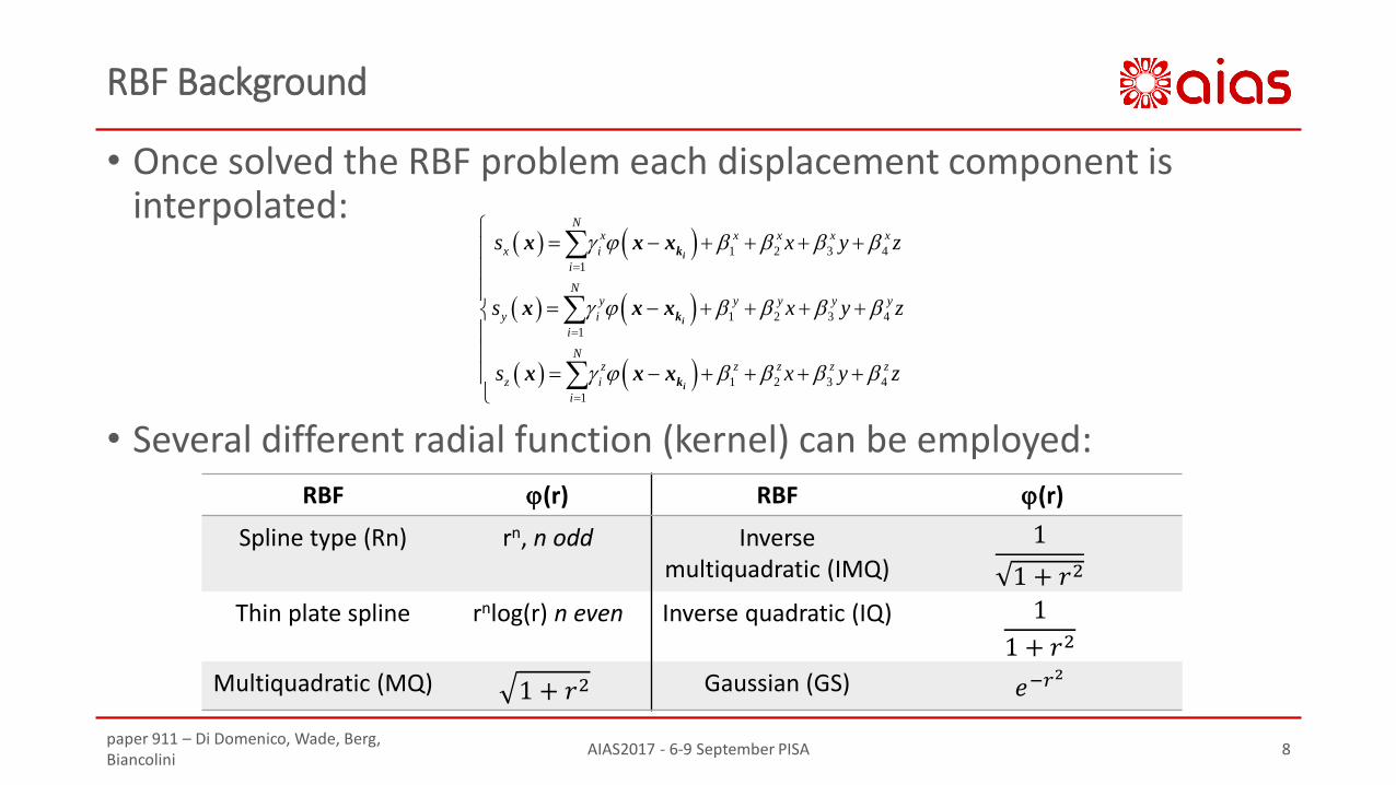
• Once solved the RBF problem each displacement component is interpolated:

• Several different radial function (kernel) can be employed:


1 2 3 4

1

1 2 3 4

1

1 2 3 4

1

Nx x x x x

x i

i

Ny y y y y

y i

i

Nz z z z z

z i

i

s x y z

s x y z

s x y z

i

i

i

k

k

k

x x x

x x x

x x x

RBF (r) RBF (r)

Spline type (Rn) rn, n odd Inversemultiquadratic (IMQ)

1

1 + 𝑟2

Thin plate spline rnlog(r) n even Inverse quadratic (IQ) 1

1 + 𝑟2

Multiquadratic (MQ) 1 + 𝑟2 Gaussian (GS) 𝑒−𝑟2


8

Structural modes embedding

• A certain number of modes is computed using FEA.

• An RBF solution is computed for each mode (constraining far field conditions and rigid surfaces, mapping FEA field on deformable surfaces). Modes on CFD mesh are stored.

• At initialization the CFD solver loads the modes and then:• the mesh deformation can be amplified

prescribing the value of modal coordinates• modal forces are computed on prescribed

surfaces by projecting the nodal forces (fluid pressure and shear) onto the modal shape


9

Structural modes embedding

• Transient analysis is performed considering the loads frozen in the time step. Each modal coordinate is updated considering the analytic equation (as usual for transient modal analyses):

• Steady analysis is performed by updating the modal coordinates at a certain number of CFD iterations (usually 20-100):

• Modes are normalized with respect to the mass (so that only the frequencies are needed).


10

𝑞 + 2𝜁𝑖𝜔𝑖 𝑞𝑖 +𝜔𝑖2𝑞𝑖 =

𝐹𝑖 𝑡

𝑀𝑖𝑖

𝜉 𝑡 = 𝑒−𝜁𝜔𝑛𝑡 𝜉0 𝑐𝑜𝑠 𝜔𝑑𝑡 + 𝜉0 + 𝜁𝜔𝑛𝜉0

𝜔𝑑𝑠𝑖𝑛 𝜔𝑑𝑡 +

1

𝑚𝜔𝑑 0

𝑡

𝑒−𝑏 𝑡−𝜏2𝑚 𝑓 𝜏 𝑠𝑖𝑛 𝜔𝑑 𝑡 − 𝜏 𝑑𝑥

𝜔𝑖2𝑞𝑖 =

𝐹𝑖𝑀𝑖𝑖

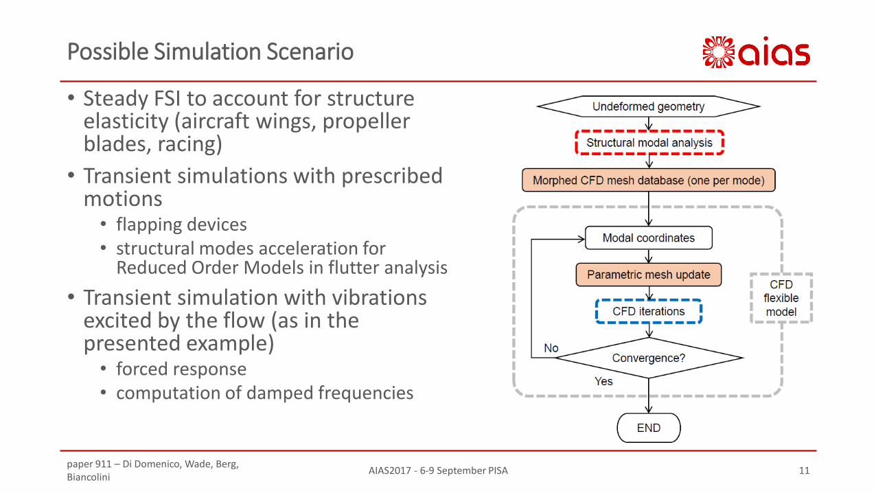
Possible Simulation Scenario

• Steady FSI to account for structure elasticity (aircraft wings, propeller blades, racing)

• Transient simulations with prescribed motions• flapping devices• structural modes acceleration for

Reduced Order Models in flutter analysis

• Transient simulation with vibrations excited by the flow (as in the presented example)• forced response• computation of damped frequencies


11

Challenges

• For very Large models (millions cells) pressure mapping and mesh update could be time consuming (Dallara GP2 example is a 250 millions mesh)

• Structural modes embedding truncation error has to be considered (especially for steady cases)

• Transient simulations can take hours (days). A robust and reliableprocess is a paramount!

• Modal superposition allows to go 10-12 times faster than two-way in transient analysis

• Modal theory is limited to linear structures.


12

Application

• NACA 0009 hydrofoil

• Angle of attack: 𝛼=0°

• Material: steel (𝜌=7850 𝑘𝑔/𝑚3)

• Constraints: embedded pivot, clamp

• Fluid: water

• References• Ausoni, P., Farhat, M., & Avellan, F. (2012). The effects of a tripped turbulent boundary layer on vortex

shedding from a blunt trailing edge hydrofoil. Journal of Fluids Engineering.

• Ausoni, P., Zobeiri, A., Avellan, F., & Farhat, M. (2009). Vortex Shedding From Blunt and Oblique Trailing Edge Hydrofoils. IAHR International Meeting of the Workgroup on Cavitation and Dynamic Problems in Hydraulic Machinery and Systems. Brno.


AIAS2017 - 6-9 September PISA 13

Application

• modes in air (ANSYS Mechanical)



Mode 1 - First bending mode

1133.8 Hz

Mode 2 - First torsional mode

1587.1 Hz

Mode 3 - Second torsional mode

3630.9 Hz

Mode 4 - Second bending mode

3917.7 Hz

Mode 5 - Third bending mode

5936.6 Hz

Mode 6 - Third torsional mode

6789.6 Hz

Application

• RBF set-up (applied to the CFD model with RBF Morph)



Lock in (predicted with ANSYS Fluent after 37h on 32 cores)

• Probe at (0.08000 m, 0.03788 m, 0.1125 m)

• Observed frequency 909.91 Hz

• Imposed speed 16 m/s

16paper 911 – Di Domenico, Wade, Berg, Biancolini


Probe vertical speed Probe vertical speed FFT

time (s)

A (

mm

/s)

Lock off (predicted with ANSYS Fluent after 37h on 32 cores)

• Probe at (0.08000 m, 0.03788 m, 0.1125 m)

• Observed frequency 1209.9Hz

• Imposed speed 22 m/s

17paper 911 – Di Domenico, Wade, Berg, Biancolini


Probe vertical speed Probe vertical speed FFT

time (s)

A (

mm

/s)

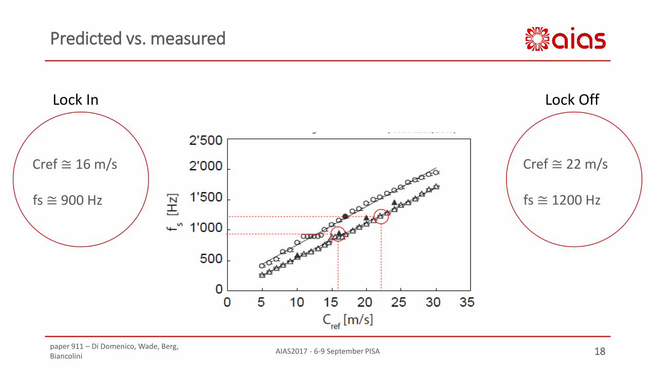
Predicted vs. measured

18

Lock In

Cref ≅ 16 m/s

fs ≅ 900 Hz

Lock Off

Cref ≅ 22 m/s

fs ≅ 1200 Hz



Modes in air vs. modes in water

• Transient response in water with initial conditions an all the modes• Modes in water computed with FFT

19

Mode 1 Mode 2 Mode 3 Mode 4 Mode 5 Mode 6

1133.8 Hz 1587.1 Hz 3660.9 Hz 3917.7 Hz 5936.6 Hz 6789.6 Hz

Mode 1 Mode 2 Mode 3 Mode 4

891.9 Hz 1118.8 Hz 1619.6 Hz 2902.7 Hz



air water

Conclusions

• In this work an FSI approach based on modal superposition based on mesh morphing techniques is presented

• Transient analysis is conducted computing modes by ANSYS Mechanical and then embedding modes within ANSYS® Fluent with RBF Morph™

• Excellent HPC performances are observed 12x vs. full two-way FSI

• A very good agreement is noticed in the ability of capturing resonances in the lock-in lock-off speed range

• The transient solver can be used for the computation of natural modes in water

• More FSI applications on RBF Morph (www.rbf-morph.com), RBF4AERO (www.rbf4aero.eu) and RIBES (www.ribes-project.eu)


20

http://www.rbf-morph.com/

http://www.rbf4aero.eu/

http://www.ribes-project.eu/

THANK YOU!


21

Fluid structure interaction analysis: vortex shedding induced vibrationsN. Di Domenico, M. E. Biancolini* University of Rome «Tor Vergata», Department of Enterprise Engineering «Mario Lucertini»

A. Wade, T. Berg,ANSYS UK, ANSYS Sweden

*[email protected]


22

fluid structure interaction analysis: vortex shedding ... · introduction •fluid structure...

Documents