investigation of multiscale fluid structure interaction
TRANSCRIPT

University of Central Florida University of Central Florida
STARS STARS
Electronic Theses and Dissertations, 2004-2019
2013
Investigation Of Multiscale Fluid Structure Interaction Modeling Of Investigation Of Multiscale Fluid Structure Interaction Modeling Of
Flow In Arterial Systems Flow In Arterial Systems
Sebastian Sotelo University of Central Florida
Part of the Mechanical Engineering Commons
Find similar works at: https://stars.library.ucf.edu/etd
University of Central Florida Libraries http://library.ucf.edu
This Masters Thesis (Open Access) is brought to you for free and open access by STARS. It has been accepted for
inclusion in Electronic Theses and Dissertations, 2004-2019 by an authorized administrator of STARS. For more
information, please contact [email protected].
STARS Citation STARS Citation Sotelo, Sebastian, "Investigation Of Multiscale Fluid Structure Interaction Modeling Of Flow In Arterial Systems" (2013). Electronic Theses and Dissertations, 2004-2019. 2580. https://stars.library.ucf.edu/etd/2580

INVESTIGATION OF MULTISCALE FLUID STRUCTURE INTERACTION MODELING
OF FLOW IN ARTERIAL SYSTEMS
by
SEBASTIAN RODRIGO SOTELO
B.S. University of Central Florida, 2012
A thesis submitted in partial fulfillment of the requirements
for the degree of Master of Science
in the Department of Mechanical and Aerospace Engineering
in the College of Engineering and Computer Science
at the University of Central Florida
Orlando, Florida
Spring Term
2013
Major Professor: Alain Kassab

ii
© 2013 Sebastian Rodrigo Sotelo

iii
ABSTRACT
The study of hemodynamic patterns in large blood vessels, such as the ascending aortic
artery, brachiocephalic trunk, right carotid artery and right subclavian artery presents the
challenging complexity of vessel wall compliance induced by the high levels of shear stress
gradients and blood flow pulsatility. Accurate prediction of hemodynamics in such conditions
requires a complete Fluid Structure Interaction (FSI) analysis that couples the fluid flow
behavior throughout the cardiac cycle with the structural response of the vessel walls. This
research focuses on the computational study of a Multiscale Fluid-Structure Interaction on the
arterial wall by coupling Finite Volumes Method (FVM) predictions of the Fluid Dynamics
within the artery with Finite Elements Method (FEM) predictions of the Elasto-Dynamics
response of the arterial walls and 1-D closed loop electrical circuit system to generate the
dynamic pressure pulse. To this end, a commercial FVM Computational Fluid Dynamics (CFD)
code (STAR-CCM+ 7.09.012) will be coupled through an external interface with a commercial
FEM Elasto-Dynamics code (ABAQUS V6.12). The coupling interface is written in such a way
that the wall shear stresses and pressures predicted by the CFD analysis will be passed as
boundary conditions to the FEM structural solver. The deformations predicted by the FEM
structural solver will be passed to the CFD solver to update the geometry in an implicit manner
before the following iteration step. The coupling between the FSI and the 1-D closed loop lump
parameter circuit updated the pressure pulse and mass flow rates generated by the circuit in an
explicit manner after the periodic solution in the FSI analysis had settled. The methodology
resulting from this study will be incorporated in a larger collaborative research program between
UCF and ORHS that entails optimization of surgical implantation of Left Ventricular Assist

iv
Devices (LVAD) cannulae and bypass grafts with the aim to minimize thrombo-embolic events.
Moreover, the work proposed will also be applied to another such collaborative project focused
on the computational fluid dynamics modeling of the circulation of congenitally affected
cardiovascular systems of neonates, specifically the Norwood and Hybrid Norwood circulation
of children affected by the hypoplastic left heart syndrome.

v
I dedicate this thesis to my loving wife that supported and encouraged me throughout my
education and believed in me each step of the way.

vi
TABLE OF CONTENTS
LIST OF FIGURES ...................................................................................................................... vii
LIST OF TABLES ......................................................................................................................... ix
CHPATER 1: INTRODUCTION ................................................................................................... 1
CHAPTER 2: LITERATURE REVIEW ........................................................................................ 4
CHAPTER 3: METHODS .............................................................................................................. 7
3.1 Computational Solid Mechanics ...................................................................................... 7
3.1.1 Hyperelastic model in ABAQUS .............................................................................. 9
3.2 Computational Fluid Dynamics ..................................................................................... 15
3.3 Fluid structure interaction coupling ............................................................................... 18
3.3.1 Co-simulation between ABAQUS and STAR-CCM+ ........................................... 18
3.4 Lumped Parameter Model .............................................................................................. 22
CHAPTER 4: RESULTS .............................................................................................................. 30
4.1 Comparison between Compliant vs. Compliant with Gore-Tex patch model .................... 34
4.2 Comparison between Compliant vs. non-Compliant model ............................................... 48
CHAPTER 5: CONCLUSION AND FUTURE WORK .............................................................. 56
APPENDIX: DERIVATIONS ...................................................................................................... 57
REFERENCES ............................................................................................................................. 60

vii
LIST OF FIGURES
Figure 1: Contrast-enhanced MR Angiography of brachiocephalic bifurcation ............................ 1
Figure 2: Histomechanical idealization of a healthy elastic artery ................................................. 7
Figure 3: Aorta 3-layer composite solid mesh .............................................................................. 12
Figure 4: Bifurcation 3-layer composite solid mesh ..................................................................... 13
Figure 5: Bifurcation 3-layer composite solid mesh with Gore-Tex patch .................................. 14
Figure 6: Aorta fluid mesh ............................................................................................................ 17
Figure 7: Bifurcation fluid mesh ................................................................................................... 17
Figure 8: Coupling of FSI and Lump parameter model ................................................................ 22
Figure 9: Generic block of vascular bed compartments ............................................................... 24
Figure 10: Bifurcation 1-D cardiovascular circuit model ............................................................. 25
Figure 11: FSI couple with lump parameter model ...................................................................... 25
Figure 12: Elastance Function and over one cardiac cycle ...................................... 27
Figure 13: Pressure and Cardiac output ........................................................................................ 29
Figure 14: Innominate, Right Carotid, and Right Subclavian Artery Pressure waveform ........... 31
Figure 15: Innominate, Right Carotid, and Right Subclavian Artery Flow rate waveform.......... 31
Figure 16: Carotid Artery Doppler images and calculated flow rate (ml/s) waveform ................ 31
Figure 17: Visualization of flow relative to Innominate artery flow rate ..................................... 34

viii
Figure 18: Wall Shear Stress of Compliant and Compliant-Gore-Tex ......................................... 37
Figure 19: RSA (right subclavian artery) and RCA (right carotid artery) cross-sections ............ 38
Figure 20: RCA cross-section velocity of Compliant and Compliant-Gore-Tex model .............. 39
Figure 21: RSA cross-section velocity of Compliant and Compliant-Gore-Tex model ............... 40
Figure 22: Velocity Field of Compliant and Compliant-Gore-Tex model ................................... 41
Figure 23: Streamlines velocity magnitude of Compliant and Compliant-Gore-Tex model ........ 42
Figure 24: Pressure of Compliant and Compliant-Gore-Tex model ............................................. 43
Figure 25: Strain of Compliant and Compliant-Gore-Tex model ................................................. 44
Figure 26: Wall Shear Stress of Compliant and non-Compliant .................................................. 50
Figure 27: RCA cross section velocity of Compliant and non-Compliant model ........................ 51
Figure 28: RSA cross section velocity of Compliant and non-Compliant model......................... 52
Figure 29: Velocity Field of Compliant and non-Compliant model ............................................. 53
Figure 30: Streamlines velocity magnitude of Compliant and non-Compliant model ................. 54
Figure 31: Pressure of Compliant and non-Compliant model ...................................................... 55

ix
LIST OF TABLES
Table 1: Parameters for the Holzapfel-Gasser-Ogden model in ABAQUS ................................. 11
Table 2: Problem size for solid domain models ............................................................................ 12
Table 3: Problem size for fluid domain models ............................................................................ 16
Table 4: Left ventricle heart, aorta, and systemic model parameters ........................................... 28
Table 5: Calculated resistance, capacitance, and inductance of arteries ....................................... 32
Table 6: Comparison of total flow rate per cycle between models ............................................... 32
Table 7: Calculated resistance, capacitance, and inductance of arterial and venous beds ............ 33
Table 8: Von Misses Stress for Compliant model ........................................................................ 45
Table 9: Von Misses Stress for Compliant with Gore-Tex model................................................ 45
Table 10: Displacement magnitude for Compliant model ............................................................ 46
Table 11: Displacement magnitude for Compliant with Gore-Tex model ................................... 46
Table 12: Wall velocity magnitude for Compliant model ............................................................ 47
Table 13: Wall velocity magnitude for Compliant with Gore-Tex model .................................... 47

1
CHPATER 1: INTRODUCTION
The study of a multiscale fluid structure interaction between three dimensional
incompressible fluid, and anisotropic hyperelastic compliant vessels has several computational
challenges. The numerical complexities that this study faces involves non-linear-anisotropic
behavior of the arterial wall, non-Newtonian fluid such as blood and strong multi-physics
coupling between the solid and fluid domain interfaces. The coupling will also need to handle a
ratio near unity of the fluid and solid density. For this particular case the subject of study is the
brachiocephalic (innominate) artery bifurcation. This thoracic artery arises from the arch of the
aorta and splits into the right subclavian (RSA) and right carotid (RCA) arteries. The right
subclavian artery supplies oxygenated blood to the right arm. The right carotid artery supplies
oxygenated blood to the head and neck areas.
(Nael, Villablanca, Pope, Laub, & Finn, 2007)
Figure 1: Contrast-enhanced MR Angiography of brachiocephalic bifurcation
Right carotid artery Right Subclavian artery
Brachiocephalic trunk

2
In this particular case study the behavior of the flow field of the blood and shear stress,
and compliance of the arterial wall will be studied using a multiscale-fluid-structure-interaction
model. The findings and methodology from this work will be used as a baseline for future
projects such as optimization of surgical implantation of Left Ventricular Assist Devices
(LVAD) cannulae and bypass grafts. This is with the aim to minimize thrombo-embolic events
by creating the computational fluid dynamics modeling of the circulation of congenitally affected
cardiovascular systems of neonates, specifically the Norwood and Hybrid Norwood circulation
of children affected by the hypoplastic left heart syndrome.
In order to achieve this goal first a CAD drawing of the bifurcation for the fluid and solid
domain was performed. The CAD file of the bifurcation geometry of the fluid and solid domains
interfaces needed to coincide in measurements. One out of the two solid domain models was
modified in order to implement a Gore-Tex patch in the right carotid artery wall. Once that was
completed the geometry was imported to the respective fluid and solid domains solver. In this
case STAR-CCM+ 7.09.012 would solve the fluid domain calculations and ABAQUS V.12 will
solve the solid domain calculations. The multi-physics co-simulation is then performed implicitly
between the fluid and solid domains by the SIMULIA Co-Simulation Engine which is ran by
ABAQUS in the background. A co-simulation script needed to be added to the ABAQUS input
file in order to perform the co-simulation between ABAQUS and STAR-CCM+. After that was
put into place the following step was used to determine the field functions that need to be
exchanged and the coupled boundaries. For this particular case the STAR-CCM+ exports static
pressures and wall shear stresses to the solid domain in ABAQUS and imports the nodal
displacement that ABAQUS calculates. The units of exchange also had to be determined. For

3
this case study the exported units from STAR-CCM+ to ABAQUS are mm and MPa. At last the
compliant bifurcation model was compare with the compliant with Gore-Tex model and the non-
compliant model to determine the changes in the flow field, pressure, and wall shear stress.
4
CHAPTER 2: LITERATURE REVIEW
The study of a multiscale fluid structure interaction of a flexible wall with large strain
deformations such as the arterial wall faces a multitude of challenges. One of the tasks involved
in performing this kind of study is its numerical complexities in solving the fluid and solid
interfaces continuity equations for a non-linear wall behavior and a non-Newtonian fluid. The
coupling algorithm must be capable of handling the multi-physics exchange of field functions
between the interfaces. The FSI also has to be coupled with a lump parameter model that updates
the boundary conditions at the inlets and outlets until the periodic waveforms settles
Regarding the study of a multiscale fluid structure interaction model of an arterial wall
Alistair G. Brown (Brown, et al., 2012) performed a computational study of the aortic
hemodynamics of the vascular system for a patient–specific aorta. In this work three different
models were studied. Each of the models was coupled with a Windkessel model (0D model) in
order to prescribe boundary conditions at the boundaries. All of the models calculated the 3D-
flow field using the computational fluid dynamic (CFD) commercial code ANSYS-CFX. One of
the models calculated the flow field by treating the fluid as an incompressible fluid. Another
model treated the fluid as a compressible fluid. The third model comprised of a fully couple fluid
structure interaction (FSI). The aortic wall was treated as a linear elastic incompressible model in
the FSI solid domain. The Windkessel model was solved using a first order backward Euler
approach. It was applied to the CFD models in an explicit manner after every time-step (5 ms) in
order to prescribe the boundary conditions. The findings of this research show that the
incompressible and compressible 3D CFD calculation of the flow field take much less time (7.8
5
hrs and 6.8 hrs) to get an adequate answer compare to the FSI model (145.5 hrs). It also shows a
higher wall shear stress at the aortic walls for the incompressible and compressible 3D CFD
calculation compare to the FSI model at early, peak, late systole and mid, end diastole. The
maximum WSS (Pa) for the FSI model were as follows: 6.01, 18.19, 17.72, 0.94, and 0.73 for
early, peak, late systole and mid, end diastole respectably.
While Brown (Brown, et al., 2012) used a liner relation for the arterial wall Xenow
(Xenow, et al., 2010) used a non-linear representation of the arterial wall. Xenow performed a
fluid structure interaction for a study in the abdominal aortic aneurysm (Xenow, et al., 2010). In
this study the parameters used to create the model were obtained from CT scans measurements
from a selected group of patients. The purpose of this work was to examine the flow field and
wall shear stress in the iliac arteries bifurcation. Different geometry parameters were used for the
purpose of developing an additional diagnostic tool to assist clinicians. In this work the
commercial computational code ADINA was used to perform the fluid and solid domain
calculations. The fluid was treated as a Newtonian fluid and the flow as laminar. The boundary
conditions prescribed in the fluid domain were a fixed velocity waveform at the inlet and
pressure wave at the outlet. For the solid domain the arterial wall was modeled using two
models. In one of the models the arterial wall was treated as an isotropic material using the
Mooney–Rivlin model. The other model used the Holzapfel orthotropic material formulation
treating the wall as an anisotropic material. The Arbitrary Lagrangian–Eulerian (ALE) approach
was used for the deformation of the fluid mesh at every time step. The fluid and solid interfaces
was coupled directly, and large strains deformations were used in the model. The arterial wall
deformations were calculated using a linear dynamics response. Both the fluid and solid domains

6
were calculated using a first order finite-element scheme. It was determined that a peak wall
shear stress (WSS) of 2.66 PA was present during peak systole at a 0 degree inlet angle. It was
also found that maximum velocity magnitude for the 120 degree bifurcation angle was 3% lower
than the maximum velocity magnitude of the 60 degree bifurcation angle geometry.

7
CHAPTER 3: METHODS
3.1 Computational Solid Mechanics
A multi-layer model for an arterial wall is centered on the mechanics of fiber-reinforced
composites theory. It represents the symmetries of a cylindrical orthotropic material. The arterial
wall is made of three major thick-walled layers (Intimia (I), media (M), and adventitia (A)).
(Holzapfel, Gasser, & Ogden, 2000)
Figure 2: Histomechanical idealization of a healthy elastic artery
Each of the layers of the arterial wall is treated as a composite reinforced by two collagen
fibers. These fibers are ordered in symmetrical spirals. It is safe to assume that each layer has
similar mechanical features. However they may have different set parameters that define the
material. Thus the same strain-energy function can be used for each layer (Holzapfel, Gasser, &
Ogden, 2000).

8
In order to represent the hyperelastic behavior of the arterial wall in the solid domain the
Holzapfel-Gasser-Ogden built-in model in ABAQUS was used. The Holzapfel model (Holzapfel,
Gasser, & Ogden, 2000) separates the strain-energy function ψ into two main parts: Ψiso and
Ψaniso which associates the isotropic (non-collagenous material matrix mechanical response) and
anisotropic (resistance to stretch at high pressures due to collagenous fibers). Thus the potential
strain-energy function is represented as follows:
ψ Ψ Ψ (1)
Where represents the distortional part of the right Cauchy-Green strain (APPENDIX:
DERIVATIONS), and the structure tensor product of which are the
two reference direction vectors of the collagenous fibers with (Holzapfel,
Gasser, & Ogden, 2000). In order to represent the response of the fibers the parameters
are describe in the following invariant-based formulation (Gasser, Ogden, &
Holzapfel, 2006).
(2)
(3)
(4)
(5)

9
Since the are constants, and represent the stretches in the direction of
which is sufficient to capture the general anisotropic mechanical behavior of the
arterial wall the strain-energy (1) can be reduced to
ψ Ψ Ψ (6)
can be represented using the neo-Hookean model for the isotropic response in
each layer as follows
Ψ
(7)
Where represents shear modulus of the material and is the first deviatoric strain
invariant of the distortional part of the right Cauchy–Green tensor .
is represented by an exponential function to describe the strain energy
stored in the collage fibers
Ψ
(8)
Where is a stress-like material parameter and is a dimensionless
parameter. These parameters do not affect the mechanical response of the arterial wall in the low
pressure domain. The invariants correspond to the square of the stretches of the fibers in
the fiber directions (Holzapfel, Gasser, & Ogden, 2000).
3.1.1 Hyperelastic model in ABAQUS
The solid models were created using the commercial code ABAQUS v6.12 Simulia.
These models were created to represent the hyperelastic properties of the arterial wall. ABAQUS
10
uses several models to represent the behavior of an anisotropic hyperelastic material. In this
particular case the Holzapfel-Gasser-Ogden built-in model was used. This hyperelastic model
combines the strain energy potential function proposed by Holzapfel, Gasser and Ogden
(Holzapfel, Gasser, & Ogden, 2000) (Gasser, Ogden, & Holzapfel, 2006) to model the arterial
layers with distributed collagen fiber orientations such that:
(9)
(10)
(11)
Where is the strain-energy potential. This functions represents the strain energy stored
per unit of reference volume;
;
( ); is the elastic volume
ratio; N refers to the number of families of fibers represents the first deviatoric strain
invariant as in equation (2). in (10) are the pseudo-invariants of (modified
Green strain tensor and unit vectors of the direction of the fibers). are the same
parameters as descript in (8). The parameter k in (11) describes the level of scattering in the fiber
directions (if fibers are perfectly aligned and fibers are randomly distributed and
the material becomes isotropic). The density is a function of the orientation of the number
of fibers in the range of (ABAQUS) (Gasser, Ogden, & Holzapfel, 2006).
The collagen fibers are only activated during tension loads since buckling could occur
under compression loads. ABAQUS uses equation (9) where and

11
in order to prevent buckling in the model (ABAQUS). The D parameter in (9) is
thus taken to be approximately zero (1E-6) in order to treat this model as an incompressible solid
since arteries can be treated as such under physiological loads (Carew, Vaishnav, & Patel, 1968).
Below table 1 shows the parameters used to model the anisotropic hyperelastic model of the
thoracic aorta in ABAQUS.
Table 1: Parameters for the Holzapfel-Gasser-Ogden model in ABAQUS
(Weisbecker, Pierce, & Holzapfel, 2012) (Lantz, Renner, & Karlsson, 2011)
Human Artery (MPa) (MPa)
Thoracic
Artery
Three-layer Composite
0.017 0.56 16.21 0.18 51.0 1080
Three different models were created, an aorta and two bifurcations (Innominate, Right
Carotid Artery, and Right Subclavian Artery). The wall thickness used in the aorta model was
2.59 mm for the three-layer composite aorta (Weisbecker, Pierce, & Holzapfel, 2012). The
dimensions for the aorta inner diameter and length are 18mm and 50 mm respectably. The
bifurcations models dimensions were as follows: constant wall thickness of 1.3mm, inner
diameters of 12.4mm for the Innominate artery, 8mm for the right subclavian artery, and 7.4mm
for the right carotid artery. To one of the bifurcation models a Gore-Tex patch near the
midsection of the right carotid artery was placed. The length of the Gore-Tex patch along the
axis is approximately 22.8mm and 10 mm radially. The patch entails of 615 quadratic tetrahedral

12
elements of type C3D10 of the bifurcation model. The Gore-Tex patch was modeled with the
following material properties Young’s’ modulus of 40 MPa and density of 3.30e-09 tonne/mm^3
(Long, Hsu, Bazilevs, Feinstein, & Marsden, 2012). A 20-node quadratic brick was used to mesh
the aorta model and a 10-node quadratic tetrahedron mesh was used to discretize the bifurcation
model.
Below table 2 contains the elements, nodes and number of variable that were solved for
the solid model in ABAQUS using the Holzapfel hyperelastic anisotropic built-in model and
figures 2 and 3 show the mesh used for the aortas and bifurcation model.
Table 2: Problem size for solid domain models
Model Elements Nodes Total Number of variables
Aorta: 3-layer-composite 2904 15718 47154
Bifurcation: 3-layer composite 11452 22567 67701
Figure 3: Aorta 3-layer composite solid mesh

13
The boundary conditions applied to the bifurcation solid domain (with and without Gore-
Tex) were as follow: 2 mm of allowable displacement on the radial direction and fixed on the
axial direction at the brachiocephalic root end face, 1.5 mm of allowable displacement on the
radial direction at the right carotid artery end face, and 1.75 mm of allowable displacement on
the radial direction at the right subclavian artery end face (APPENDIX: DERIVATIONS). The
boundary conditions were referenced to a local coordinate system created at the center of each of
the faces. The solid domain was solved using ABAQUS dynamic-quasi-static solver with a
velocity parabolic extrapolation.
Figure 4: Bifurcation 3-layer composite solid mesh
Brachiocephalic
root
Right Subclavian
Artery
Right Carotid Artery

14
Figure 5: Bifurcation 3-layer composite solid mesh with Gore-Tex patch
22.8 mm -10 mm

15
3.2 Computational Fluid Dynamics
The segregated flow formulation was used in STAR-CCM+ to solve the continuity and
momentum governing equations. For this particular model the fluid (blood) was treated as
Laminar, Newtonian and incompressible fluid with a constant density of 1060 kg/m3 and a
dynamic viscosity of 0.004 Pa-s. Gravitational forces were neglected.
(12)
(13)
The governing equations were discretized using a Finite Volume Discretization method.
For the momentum equation applying a cell-centered control volume for cell-0:
(14)
Where the left hand side of (14) represents the transient terms and convective flux. The
right hand side represents the pressure gradient, viscous flux and the body force terms. T in (14)
is the viscous stress tensor. T is equal to the laminar stress tensor for this case since a turbulent
model was not used.
(15)
(16)

16
The velocity gradient tensor ( ) is written in terms of the cell velocities in order to
evaluate the stress tensor (T). The velocity gradient tensor at the interior face is then written as
follows:
(17)
(18)
(19)
Where and are computed (explicitly) velocity gradient tensor in the cells. For the
boundary face the no-slip condition is used. An unsteady, implicit, second order solver was used
to solve the Navier-Stokes equation with a time-step of 0.005 sec. The following boundary
conditions were imposed on the boundaries: inlet unsteady stagnation pressure on the Innominate
Artery face and outlet unsteady mass flow rate on the Right Carotid Artery and Right Subclavian
Artery. These boundary conditions were calculated using a 1-D lumped parameter model
described in the section 3.4 . The floating morpher boundary type method was used for the
Innominate, Right Carotid, and Right Subclavian faces. This method allows for the boundaries to
be only a function of solid domain boundary conditions.
Table 3: Problem size for fluid domain models
Model Cells
Aorta: 3-layer-composite 27764
Bifurcation: 3-layer composite 91160

17
Figure 6: Aorta fluid mesh
Figure 7: Bifurcation fluid mesh

18
3.3 Fluid structure interaction coupling
This FSI contains two domains and for the solid and fluid respectably. These two
domains do not overlap and are share by a common interface . The information exchanged
between these two domains are the pressure p (traction vector: wall shear stress and static
pressure) from the fluid domain and the displacement d (nodal displacement) from the solid
domain for this particular case. The exchanged of these unknowns (p and d) occurs at the shared
interface and thus becoming the coupling of the solid and fluid domains (Kuttler & Wall, 2008).
Kinematic and dynamic continuity are both fulfilled at all times during the coupling process. In
the case of non-slip conditions at the interface
(20)
The stresses equal at the deformed interface based on the kinematic continuity where n is
the time dependent interface normal. represents the interface displacement. The interface
displacement changes the interface position as such . (Kuttler & Wall, 2008).
3.3.1 Co-simulation between ABAQUS and STAR-CCM+
In order to perform the fluid structure interaction (FSI) for this model the commercial
software STAR-CCM+ 7.06 CD-adapco and ABAQUS v6.12 SIMULIA were used. STAR-
CCM+ was used to solve the fluid domain and ABAQUS the solid domain in this particular FSI
model. Each model was first solved individually (no co-simulation) in order to determine if there
were any numerical problems. The co-simulation was carried by the SIMULIA Co-simulation
engine. The SIMULIA Co-Simulation Engine is responsible for communication between Abaqus
and STAR-CCM+. This Engine allows ABAQUS to perform a run-time coupling with a third

19
party program (CFD) to solve a multiphysisc simulation and multidomain coupling and it runs in
the background of the simulation (ABAQUS).
STAR-CCM+ uses a mesh motion called morphing in order to deform the interface (Γ) at
the fluid domain in accordance to the imported nodal displacements calculated in ABAQUS. The
fluid grid deforms accordantly in order to match the solid structure as well as maintaining a
reasonable mesh quality. STAR-CCM+ refers this to as a “topologically constant” operation. The
mesh motion in STAR-CCM+ uses a multi-quadric morphing model based on radial basis
functions. The morphing defines the motion of interior vertices, which originates from the
motion of the vertices on the structural surface and the fluid transport equations are solved using
the space conservation law in order to account for the motion of the mesh (STAR-CCM+).
In order to utilize the SIMULIA Co-Simulation Engine the ABAQUS input file has to be
modified with the following script: *CO-SIMULATION, NAME=<>, PROGRAM=
MULTIPHYSICS, CONTROLS=<>. Under CONTROLS it defines the coupling and
rendezvousing schemes that controls the co-simulation. The MULTIPHISICS program allows
exchange data with third-party analysis programs that support the SIMULIA Co-Simulation
Engine.
It is important to identify the interface (Γ) in both the fluid and solid domain. For the
solid domain the following script needs to be added:
*CO-SIMULATION REGION, TYPE=SURFACE, EXPORT
ASSEMBLY_FSI_INTERFACE, U

20
*CO-SIMULATION REGION, TYPE=SURFACE, IMPORT
ASSEMBLY_FSI_INTERFACE, CF
Where the identified interface is called FSI_INTERFACE and it is exporting U (nodal
displacement) and is importing CF (Traction vector: wall shear stress and static pressure) in this
particular FSI model.
The next step is to determine the coupling scheme for the exchange of data between
ABAQUS and STAR-CCM+. There are currently three choices: JACOBI (explicit parallel
coupling), GAUSS-SEIDEL (explicit serial coupling), and ITERATIVE (implicit serial
coupling). The script should also be added to the ABAQUS input file as follows: *CO-
SIMULATION CONTROLS, NAME=<>, COUPLING SCHEME=ITERATIVE, SCHEME
MODIFIER=LEAD. For this FSI model the ITERATIVE coupling scheme was chosen. The
SCHEME MODIFIER is used in the serial coupling and in this case ABAQUS was chosen to
lead the co-simulation.
It is also necessarily to determine a coupling time step. Thus the next section is added to
the *CO-SIMULATION CONTROLS script: STEP SIZE=IMPORT. There are five choices for
the coupling time step: constant, minimum, maximum, import and export. IMPORT was chosen
for this particular. This means that ABAQUS can import the suggested coupling time step from
STAR-CCM+.
Another parameter that is needed in the SIMULIA Co-Simulation Engine is the
controlling of the ABAQUS time incrementation. This parameter is selected as follows: TIME

21
INCREMENTATION=SUBCYCLE. The SUBCYCLE parameter allows ABAQUS to use its
own time incrementation in order to arrive to the target coupling time. This selection is not
recommended for implicit coupling since the iterative coupling between the two domains (fluid
and solid) will be performed in the last subcycled time step, but it is necessary to use since there
is a non-linear deformation in the solid domain. The other option is the LOCKSTEP command
which keeps a constant time-step for the solid domain solution. The problem with this choice is
that for a non-linear deformation ABAQUS may require smaller time-steps than the prescribed
one and thus there is a very high chance that solution will converge.
Another parameter that is added to the co-simulation script is the target time. This
parameter is enforced as follows: TIME MARKS=YES. There are two options YES/NO
meaning that ABAQUS will exchange data in an exact manner or not (see APPENDIX:
DERIVATIONS for final script)

22
3.4 Lumped Parameter Model
An electrical analog was developed, using the Greenfield-Fry's electrical analogy, to
simulate pulsatile flow behavior of the human circulatory system. This closed loop circuit was
coupled with the fluid structure interaction simulation in order to update the boundary conditions
at the inlet and outlets of the fluid domain. This set up allowed for the system (Fluid-solid-
lumped parameter model) to behave as complete closed system which closely replicates the
behavior of the cardiovascular system (Ceballos, 2011).
Figure 8: Coupling of FSI and Lump parameter model
This solutions begins from the Navier-Stokes equation using cylindrical coordinates
where r is radial direction variable, u is the velocity in the x-direction, t is time, μ is the dynamic
viscosity, P is the pressure, and ν is the kinematic viscosity.
(21)
FSI 1-D Circuit

23
Multiplying and integrating both sides of equation (21) by 2πrdr and from zero to R
where R is the inner radius of the tube respectably leads to equation (22) after some algebraic
manipulation.
(22)
And for a Newtonian fluid the wall shear stress can be represented as follows:
(23)
Taking equations (22) and (23) leads to equation (24) after some manipulation
(24)
Equation (24) can be further simplified by assuming a Poiseuille flow which allows the
wall shear to be expressed as follows:
(25)
Where Q is the flow rate and R the inner radius of the vessel. Equation (24) then becomes
(26)
Equation (26) can then be expressed as follows
(27)

24
Where Lu and Rv are the vascular inductance and resistance. cu and cv are constants
typically found by experiment. They arise from the assumption that in a Poiseuille flow the wall
shear stress is depended on
(28)
(29)
In order to express the compliance that occurs on the vessel a capacitor is used as an
analogous. Thus the flow rate that passes through the capacitor can be represented as follows.
(30)
(31)
Figure 9: Generic block of vascular bed compartments
For this particular of lump parameter model only the left ventricle of the heart was model.
The heart was modeled with a time dependent capacitor which is the driving function of the
circuit. The volume modulus of elasticity is equal to the reciprocal of the time dependent
capacitor which provides the pulsatile flow needed in the circuit.

25
Figure 10: Bifurcation 1-D cardiovascular circuit model
Figure 11: FSI couple with lump parameter model

26
The time dependant capacitor shown in Figure 10 represents the left ventricle compliance
(C(t)) which equals the reciprocal of the elastance (E(t)). For this research the “double hill”
elastance function was used (Simaan, Ferreira, Chen, Antaki, & Galati, 2009).
(32)
(33)
(34)
represents the normalized elastance as a function of which is defined in
equation (33). in equation (33) represents the cardiac cycle interval (60/HR and HR is the heart
rate). For the values of Emax and Emin 2 and 0.06 mmHg/ml were used respectably with a
heartbeat of 70 beats per minute. The parameters used to model the left ventricle of the heart are
shown in below in Table 4. The and plots in Figure 12 match the plots used in
Simaan’s work (Simaan, Ferreira, Chen, Antaki, & Galati, 2009).
For this particular case nineteen first order differential equations were solved using the
Runge-Kutta 4th
order adaptive solver function in MathCAD. The periodic solution was ran for
thirteen cycles before it converge The pressure waveform for the ventricular, atrial, and aorta
root pressure are shown in Figure 13 as well as the flow rate waveform of the cardiac output.
These pressure and flow rate waveform are of similar shape and magnitude as the ones found in
Simaan’s study (Simaan, Ferreira, Chen, Antaki, & Galati, 2009).

27
Figure 12: Elastance Function and over one cardiac cycle

28
Table 4: Left ventricle heart, aorta, and systemic model parameters
(Simaan, Ferreira, Chen, Antaki, & Galati, 2009) (Ottese, Olufsen, & Larsen, 2004)
(Lagana, et al., 2005)
Physiological meaning Value Units Parameter
Left Atrial Elastance 0.075 C_LA
Mitrial Valve Resistance 0.005 R_MV
Mitrial Valve D_M
Left Ventricular Compliance Time dependant C(t)
Aortic Valve Resistance 0.001 R_AV
Aortic Valve D_A
Aorta Capacitance 0.08 C_AO
Aorta Resistance 0.0398 R_AO
Aorta Inductance 0.0005 L_AO
Systemic resistance 1 R_systemic
RCA venous bed Inductance 0.001069 L_RCAv
RSA venous bed Inductance 0.001069 L_RSAv

29
Figure 13: Pressure and Cardiac output

30
CHAPTER 4: RESULTS
As mentioned above, the bifurcation compliant model was studied. This model comprises
of the brachiocephalic trunk, right carotid and right subclavian arteries. It was then compared to
the compliant with Gore-Tex model and the non-compliant model in order to study the changes
in the flow field, pressure and wall shear stress. The compliant model ran for twenty FSI-1D
circuit iterations before it reached convergence. The final calculated values for the innominate,
right carotid and right subclavian arteries are shown in Table 5. Table 6 contains the total flow
rate calculated for each of the three models. The arterial and venous beds values are found in
Table 7 as well as the systemic resistance and capacitance. The standard deviation and mean of
the characteristic impedance of the brachiocephalic trunk, right carotid artery and right
subclavian artery were as follows 0.006, 0.026, 0.012 and 0.214 , 1.134
, 0.270 respectably. The percent changed of cardiac output was << 2%.
Figure 14 and Figure 15 show the results of the pressure and flow rate waveforms in the
brachiocephalic, right carotid, and right subclavian artery. Figure 16 compares the calculated
right carotid artery waveform with a Doppler sample waveform. It can be noticed from Figure 16
the similarities in the calculated waveform and the Doppler sample. The black/white dots
represent the peaks and dips of the wave in one cycle. It was also noticed that the total output
increased as the models became more rigid. The aorta model was used to test the boundary
conditions and material properties applied to the fluid and solid domains. It was also used to
validate the FSI simulation. The pressure wave velocity (PWS) in the aorta was calculated for
one cycle. It equals 7.2 m/s using the parameters given in the methods section which is within
range according to Caro (Caro, Pedley, Schroter, & Seed, 2012).

31
Figure 14: Innominate, Right Carotid, and Right Subclavian Artery Pressure waveform
Figure 15: Innominate, Right Carotid, and Right Subclavian Artery Flow rate waveform
(Simens-Healthcare)
Figure 16: Carotid Artery Doppler images and calculated flow rate (ml/s) waveform

32
Table 5: Calculated resistance, capacitance, and inductance of arteries
Physiological meaning Value Units Parameter
Innominate Artery Resistance 0.015 R_IA
Innominate Artery Capacitance 0.0596 C_IA
Innominate Artery Inductance 0.002 L_IA
Right Carotid Artery Resistance 0.058 R_RCA
Right Carotid Artery Capacitance 0.007 C_RCA
Right Carotid Artery Inductance 0.006 L_RCA
Right Subclavian Resistance 0.018 R_RSA
Right Subclavian Capacitance 0.059 C_RSA
Right Subclavian Inductance 0.003 L_RSA
Aorta Inductance 0.0006 L_AO
Table 6: Comparison of total flow rate per cycle between models
Model
Compliant Compliant with
Gore-Tex Patch Non-Compliant
Outp
ut
(cc
/min
) Right Carotid Artery 457.51 458.23 466.47
Right Subclavian Artery 417.62 418.27 425.78
Systemic 4582 4588 4685
Total 5457.13 5464.5 5577.25

33
Table 7: Calculated resistance, capacitance, and inductance of arterial and venous beds
Physiological meaning Value Units Parameter
RCA arterial bed Resistance 10.61 R_RCAb
RCA arterial bed Capacitance 0.02 C_RCAb
RCA arterial bed Inductance 0.02 L_RCAb
RSA arterial bed Resistance 11.66 R_RSAb
RSA arterial bed Capacitance 0.02 C_RSAb
RSA arterial bed Inductance 0.02 L_RSAb
Systemic Capacitance 1.05 C_systemic
Systemic Resistance 1.22 R_systemic
RCA venous bed Resistance 1.51 R_RCAv
RCA venous bed Capacitance 0.007 C_RCAv
RSA venous bed Resistance 1.66 R_RSAv
RSA venous bed Capacitance 0.007 C_RSAv

34
4.1 Comparison between Compliant vs. Compliant with Gore-Tex patch model
The compliant and compliant with Gore-Tex patch models were ran for four cycles (1
cycle = 0.857 secs) each for total time of 3.43 seconds for each simulation. The last iteration of
boundary conditions from the 1-D lump parameter was used for these FSI simulations. In order
to visualize the difference in the wall shear stress, flow field and pressure gradients four different
times were selected within a cycle.
Figure 17 shows the different times selected to represent the comparison between these
models.
Figure 17: Visualization of flow relative to Innominate artery flow rate
There was an increased in the wall shear stress mainly in the right carotid artery where
the patch was placed at t=0.18 sec as it is shown in Figure 18. The max. average wall shear stress
value calculated in the Gore-Tex patch area is approx. 16.5 dyne/cm^2 . It is found in almost the
entire right carotid artery. As the flow rate started to decrease at t=0.36 sec a high shear stress
t1=0.05 s
t2=0.18 s
t3=0.36
t4=0.60 s 0
5
10
15
20
25
30
35
40
45
0 0.2 0.4 0.6 0.8
Flo
w R
ate
(m
l/s)
Time (s)

35
(~13 dyne/cm^2) is noticeable in the transition area between the arterial wall and the patch
coming from the bifurcation.
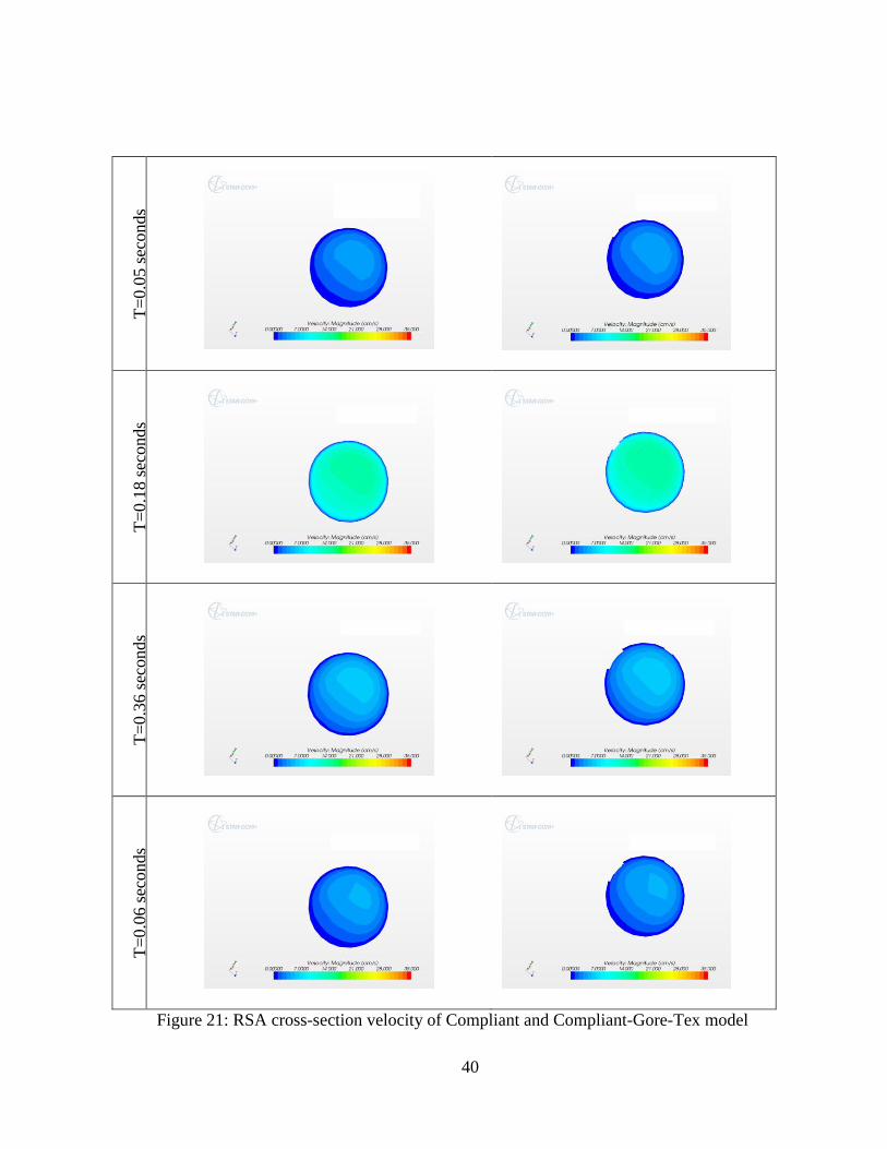
It was noticed that in the cross-section of the right carotid artery in Figure 20 the max.
average velocity was ~42 cm/s in the patch area compared to ~30 cm/s in the compliant model at
t=0.18 sec. The flow fields are of similar shape and magnitude for the compliant and compliant
with Gore-Tex model in the cross-section view of the right subclavian artery shown in Figure 21.
The velocity average calculated at peak time (t=0.18 sec) shown in Figure 22 was ~24 cm/s and
~32 cm/s at the innominate root for the compliant Gore-Tex and compliant model respectably. It
was also noticed that the velocity increased in the arterial wall-patch transition section. The
velocity maintained a maximum value of ~42 cm/s thought-out the patch section. It then
decreased to~34 cm/s after exiting the Gore-Tex patch area. This is shown in Figure 22 at
t=0.18sec. Recirculation was also noticed for both models in Figure 22 at t=0.05sec. This
recirculation was observed at the midsection of the right subclavian artery away from the
bifurcation.
The pressure contours in Figure 24 show that there was an increased of pressure at the
root of the innominate trunk for the entire cycle in the compliant Gore-Tex model. At t=0.05 sec
about half of the innominate trunk was about 71.13 mmHg in compliant Gore-Tex model while
the compliant model had 71.1 mmHg. At t=0.18 sec the pressure in the right carotid artery was
approximately 89.8 mmHg for most of the artery in patch section. There was a very small
pressure gradient variation from the bifurcation to the artery wall-patch transition section. While

36
the compliant model at t=0.18 sec shows at smoother pressure gradient transition from the
bifurcation to the right carotid artery outlet.
.

37
T=
0.0
5 s
econds
T=
0.1
8 s
econds
T=
0.3
6 s
econds
T=
0.0
6 s
econds
Figure 18: Wall Shear Stress of Compliant and Compliant-Gore-Tex

38
Figure 19: RSA (right subclavian artery) and RCA (right carotid artery) cross-sections

39
T=
0.0
5 s
econds
T=
0.1
8 s
econds
T=
0.3
6 s
econds
T=
0.0
6 s
econ
ds
Figure 20: RCA cross-section velocity of Compliant and Compliant-Gore-Tex model
40
T=
0.0
5 s
econds
T=
0.1
8 s
econds
T=
0.3
6 s
econds
T=
0.0
6 s
econds
Figure 21: RSA cross-section velocity of Compliant and Compliant-Gore-Tex model

41
T=
0.0
5 s
econds
T=
0.1
8 s
econds
T=
0.3
6 s
econds
T=
0.0
6 s
econds
Figure 22: Velocity Field of Compliant and Compliant-Gore-Tex model

42
T=
0.0
5 s
econds
T=
0.1
8 s
econds
T=
0.3
6 s
econds
T=
0.0
6 s
econds
Figure 23: Streamlines velocity magnitude of Compliant and Compliant-Gore-Tex model

43
T=
0.0
5 s
econds
T=
0.1
8 s
econds
T=
0.3
6 s
econds
T=
0.0
6 s
econds
Figure 24: Pressure of Compliant and Compliant-Gore-Tex model

44
T=
0.0
5 s
econds
T=
0.1
8 s
econds
T=
0.3
6 s
econds
T=
0.0
6 s
econds
Figure 25: Strain of Compliant and Compliant-Gore-Tex model

45
Table 8: Von Misses Stress for Compliant model
Von Misses Stress (MPA)
Time (sec) IA RCA RSA
0.05 0.080 0.042 0.089
0.18 0.100 0.053 0.114
0.36 0.121 0.066 0.140
0.60 0.101 0.054 0.115
Table 9: Von Misses Stress for Compliant with Gore-Tex model
Von Misses Stress (MPA)
Time (sec) IA RCA RSA
0.05 0.076 0.036 0.090
0.18 0.096 0.048 0.116
0.36 0.116 0.060 0.141
0.60 0.097 0.049 0.116

46
Table 10: Displacement magnitude for Compliant model
Displacement magnitude (mm)
Time (sec) IA RCA RSA
0.05 0.034 0.046 0.023
0.18 0.218 0.272 0.150
0.36 0.375 0.515 0.284
0.60 0.234 0.322 0.177
Table 11: Displacement magnitude for Compliant with Gore-Tex model
Displacement magnitude (mm)
Time (sec) IA RCA RSA
0.05 0.017 0.016 0.010
0.18 0.220 0.070 0.185
0.36 0.402 0.162 0.414
0.60 0.329 0.268 0.440

47
Table 12: Wall velocity magnitude for Compliant model
Wall velocity magnitude (mm/s)
Time (sec) IA RCA RSA
0.05 0.727 0.853 0.547
0.18 6.191 9.157 6.378
0.36 1.027 0.683 0.481
0.60 0.943 1.279 0.845
Table 13: Wall velocity magnitude for Compliant with Gore-Tex model
Wall velocity magnitude (mm/s)
Time (sec) IA RCA RSA
0.05 0.739 0.486 0.467
0.18 4.843 3.862 6.287
0.36 0.899 0.940 0.425
0.60 0.888 0.324 0.591

48
4.2 Comparison between Compliant vs. non-Compliant model
The compliant and non-compliant models were ran for four cycles (1 cycle = 0.857 secs)
each for total time of 3.43 seconds for each simulation. The last iteration of boundary conditions
from the 1-D lump parameter was used for these FSI simulations. In order to visualize the
difference in the wall shear stress, flow field and pressure gradients four different times were
selected within a cycle.
Figure 17 shows the different times selected to represent the comparison between these
models.
There was an increased in the wall shear stress almost throughout the whole bifurcation
system at t=0.18 sec as it is shown in Figure 26. The max. average wall shear stress value
calculated in the non-compliant model at this time was approx. 36.5 dyne/cm^2. As the flow rate
started to decrease at t=0.36 sec a high shear stress (~16-13 dyne/cm^2) is noticeable throughout
the right carotid artery wall.
It was noticed that in the cross-section of the right carotid artery in Figure 27 the max.
average velocity was ~63 cm/s in the non-compliant model compared to ~30 cm/s in the
compliant model at t=0.18 sec. The flow fields shown in Figure 28 indicate that there was an
increased of velocity in the right subclavian. The non-compliant model shows at t=0.18 sec a
maximum velocity of ~31.5 cm/s while the compliant model was showing ~17.5 cm/s for
maximum velocity. The velocity average calculated at peak time (t=0.18 sec) shown in Figure 29
was ~40 cm/s and ~32 cm/s at the innominate root for the non-compliant and compliant model
respectably. It was also noticed that the velocity increased throughout the entire cardiac cycle in
49
the non-compliant model. A velocity of ~45 cm/s was impinging at the bifurcation junction in
the non-compliant model compare to ~20 cm/s in the compliant model. The velocity maintained
a maximum value of ~40 cm/s throughout innominate artery and increased as it shifted to the
right carotid artery to ~69 cm/s. This is shown in Figure 29 at t=0.18sec. A recirculation was also
noticed for both models in Figure 29 at t=0.05sec. This recirculation was observed at the
midsection of the right subclavian artery away from the bifurcation.
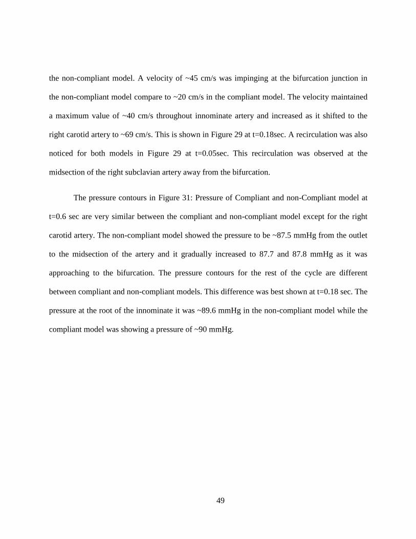
The pressure contours in Figure 31: Pressure of Compliant and non-Compliant model at
t=0.6 sec are very similar between the compliant and non-compliant model except for the right
carotid artery. The non-compliant model showed the pressure to be ~87.5 mmHg from the outlet
to the midsection of the artery and it gradually increased to 87.7 and 87.8 mmHg as it was
approaching to the bifurcation. The pressure contours for the rest of the cycle are different
between compliant and non-compliant models. This difference was best shown at t=0.18 sec. The
pressure at the root of the innominate it was ~89.6 mmHg in the non-compliant model while the
compliant model was showing a pressure of ~90 mmHg.

50
T=
0.0
5 s
econds
T=
0.1
8 s
econds
2.
T=
0.3
6 s
econds
T=
0.0
6 s
econds
Figure 26: Wall Shear Stress of Compliant and non-Compliant

51
T=
0.0
5 s
econds
T=
0.1
8 s
econds
T=
0.3
6 s
econds
T=
0.0
6 s
econds
Figure 27: RCA cross section velocity of Compliant and non-Compliant model

52
T=
0.0
5 s
econds
T=
0.1
8 s
econds
T=
0.3
6 s
econds
T=
0.0
6 s
econds
Figure 28: RSA cross section velocity of Compliant and non-Compliant model

53
T=
0.0
5 s
econds
T=
0.1
8 s
econds
T=
0.3
6 s
econds
T=
0.0
6 s
econds
Figure 29: Velocity Field of Compliant and non-Compliant model

54
T=
0.0
5 s
econds
T=
0.1
8 s
econds
T=
0.3
6 s
econds
T=
0.0
6 s
econds
Figure 30: Streamlines velocity magnitude of Compliant and non-Compliant model

55
T=
0.0
5 s
econds
T=
0.1
8 s
econds
T=
0.3
6 s
econds
T=
0.0
6 s
econds
Figure 31: Pressure of Compliant and non-Compliant model

56
CHAPTER 5: CONCLUSION AND FUTURE WORK
This study shows that multiscale fluid structure interactions with a closed loop lump
parameter have an effect on important clinical parameters such as wall shear stress, flow fields
and pressures. Furthermore this research shows the behavior of the anisotropic hyperelastic
arterial wall has when a material such as Gore-Tex, with much larger elastic properties, is
introduced to the solid domain and the impact it has on the flow field. The methodology used in
this work brings us a step closer in accurately modeling hemodynamic patterns in large blood
vessels when arterial wall motion is taken into consideration. This work will be applied to the
computational fluid dynamics modeling of the circulation of congenitally affected cardiovascular
systems of neonates, specifically the Norwood and Hybrid Norwood circulation of children
affected by the hypoplastic left heart syndrome. Moreover, this study will be used for the
optimization of surgical implantation of Left Ventricular Assist Devices (LVAD) cannulae and
bypass grafts with the aim to minimize thrombo-embolic events.
Future work should implement a patient specific anatomy instead of a synthetic model in
order to provide an investigation to a particular case of study. Also, material properties that can
be used to describe an anisotropy hyperelastic model of neonatal blood vessels.

57
APPENDIX: DERIVATIONS

58
Kinematics
, where F is defined into a spherical part and a unimodular part ,
and the .Then the Cauchy-Green tensors can be written as:
Where C and b are the right and left Cauchy-Green tensors, and and the modified
counterparts (Gasser, Ogden, & Holzapfel, 2006).
Bifurcation Boundary Conditions
**
** BOUNDARY CONDITIONS
**
** Name: BC-IA Type: Displacement/Rotation
*Boundary
IA, 1, 1, 2
IA, 2, 2, 2
IA, 3, 3
** Name: BC-RCA Type: Displacement/Rotation
*Boundary
RCA, 1, 1, 1.5
RCA, 2, 2, 1.5
** Name: BC-RSA Type: Displacement/Rotation
*Boundary
RSA, 1, 1, 1.75
RSA, 2, 2, 1.75

59
Co-simulation final script
*CO-SIMULATION, NAME=AORTA, PROGRAM=MULTIPHYSICS,CONTROLS=Control
*CO-SIMULATION REGION, TYPE=SURFACE, EXPORT
ASSEMBLY_FSI_INTERFACE, U
*CO-SIMULATION REGION, TYPE=SURFACE, IMPORT
ASSEMBLY_FSI_INTERFACE, CF
*CO-SIMULATION CONTROLS, NAME=Control, COUPLING SCHEME=ITERATIVE, SCHEME
MODIFIER=LEAD, STEP SIZE=IMPORT, TIME INCREMENTATION=SUBCYCLE, TIME MARKS=YES

60
REFERENCES
ABAQUS, V6.12 .. (n.d.). Abaqus Analysis User's Manual: 22.5.3 Anisotropic hyperelastic
behavior.
Brown, A. G., Shi, Y., Marzo, A., Staicu, C., Valverde, I., Beerbaum, P., et al. (2012). Accuracy
vs.computationaltime:Translatingaorticsimulationstotheclinic. Journal of Biomechanics
45, 516-523.
Carew, T. E., Vaishnav, R. N., & Patel, D. J. (1968). Compressibility of the Arterial Wall. Circ
Res. , 23:61-68.
Caro, C. G., Pedley, T. J., Schroter, R. C., & Seed, W. A. (2012). The Mechanics of the
Circulation. United Kingdom: Cambridge University Press.
Ceballos, A. (2011). A MULTISCALE MODEL OF THE NEONATAL CIRCULATORY SYSTEM
FOLLOWING HYBRID NORWOOD PALLIATION. Orlando: University of Central
Florida.
Gasser, T. C., Ogden, R. W., & Holzapfel, G. A. (2006). Hyperelastic modelling of arterial
layers with distributed collagen fibre orientations. J.R. Soc. Interface , 3:15-35.
Holzapfel, G. A., Gasser, T. C., & Ogden, R. W. (2000). A new constitutive framework for
arterial wall mechanics and a comparative study of material models. J. Elasticity , 61:1-
48.
Kuttler, U., & Wall, W. A. (2008). Fixed-point fluid-structure interaction solver with dynamic
relaxation. Comput Mech , 43:61-72.
Lagana, K., Balossino, R., Migliavacca, F., Pennati, G., Bove, E. L., de Leval, M. R., et al.
(2005). Multiscale modeling of the cardiovascular system: application to the study of
pulmonary and coronary perfusion in the unventricular circulation. Journal of
Biomechanics 38, 1129-1141.

61
Lantz, J., Renner, J., & Karlsson, M. (2011). WALL SHEAR STRESS IN A SUBJECT
SPECIFIC HUMAN AORTA — INFLUENCE OF FLUID-STRUCTURE
INTERACTION. International Journal of Applied Mechanics Vol. 3 No. 4 , 759-778.
Long, C. C., Hsu, M. -C., Bazilevs, Y., Feinstein, J. A., & Marsden, A. L. (2012). Fluid–
structure interaction simulations of the Fontan procedure using variable wall properties.
INTERNATIONAL JOURNAL FOR NUMERICAL METHODS IN BIOMEDICAL
ENGINEERING, 28:513-527.
Nael, K. M., Villablanca, J. P., Pope, W. B., Laub, G. P., & Finn, J. P. (2007). Supraaortic
Arteries: Contrast-enhanced MR Angiography at 3.0 T-Highly Accelerated Parallel
Acquisition for Improved Spatial Resolution over an Extended Field of View. Radiology,
242,600-609.
Ottese, J. T., Olufsen, M. S., & Larsen, J. K. (2004). Applied Mathematical Models in Human
Physiology. Philadelphia: Siam.
Simaan, M. A., Ferreira, A., Chen, S., Antaki, J. F., & Galati, D. G. (2009). A Dynamical State
Space Respresentation and Performance Analysis of a Feedback-Controlled Rotary Left
Ventricualr Assist Device. IEEE TRANSACTIONS ON CONTROL SYSTEMS
TECHNOLOGY, Vol. 117, NO.1.
Simens-Healthcare. (n.d.). Retrieved 3 23, 2013, from http://www.medical.siemens.com:
http://www.medical.siemens.com/siemens/en_US/rg_marcom_FBAs/images/presskits/A
CC_2008/USD/X300_CCA_Doppler.jpg
STAR-CCM+. (n.d.). STAR-CCM+ User Guide version 7.06.
Weisbecker, H., Pierce, D. M., & Holzapfel, G. A. (2012). Layer-specific damage experiments
and modeling of human thoraci and abdominal aortas with non-atherosclerotic intimal
thickening. Journal of the Mechanical Behavior of Biomedical Materials , 12:93-106.

62
Xenow, M., Alemu, Y., Zamfir, D., Einav, S., Ricotta, J. J., Labropoulos, N., et al. (2010). The
effect of angulation in abdominal aortic aneurysms: fluid–structure interaction
simulations of idealized geometries. Med Biol Eng Comput.