flow-3d ymuz2 linux, version 1.0 (installation and ... · flow-3d version 9.2 (flow science, inc.,...
TRANSCRIPT

INSTALLATION AND VALIDATION TEST REPORT FOR FLOW-3D YMUZ2 LINUX, VERSION 1.0
Prepared by
Kaushik Das Debashis Basu
Center for Nuclear Waste Regulatory Analyses® San Antonio, Texas
July 2008

ii
CONTENTS Section Page
CONTENTS .................................................................................................................................. ii FIGURES..................................................................................................................................... iv TABLES ....................................................................................................................................... vi
1 INTRODUCTION ......................................................................................................................1 1.1 Background ...........................................................................................................2 1.2 Scope of Regression Tests ...................................................................................3
2 ENVIRONMENT .......................................................................................................................4 2.1 Hardware Requirements .......................................................................................4 2.2 Software for the Baseline Flow Solver ..................................................................4 2.3 Installation of FLOW-3D YMUZ2 Linux .................................................................4 2.4 Running FLOW-3D YMUZ2 Linux Version 1.0 in Parallel Environment ...............5
3 PREREQUISITES.....................................................................................................................7
4 ASSUMPTIONS AND CONSTRAINTS ....................................................................................7
5 NATURAL AND FORCED CONVECTION ...............................................................................7 5.1 Laminar Natural Convection on a Vertical Surface ...............................................7
5.1.1 Test Input....................................................................................................7 5.1.2 Expected Test Results................................................................................7 5.1.3 Test Results................................................................................................7
5.2 Turbulent Natural Convection in an Air-Filled Square Cavity ..............................11 5.2.1 Test Input..................................................................................................11 5.2.2 Expected Test Results..............................................................................12 5.2.3 Test Results..............................................................................................12
5.3 Natural Convection in an Annulus Between Horizontal Concentric Cylinders....17 5.3.1 Test Input..................................................................................................17 5.3.2 Expected Test Results..............................................................................17 5.3.3 Test Results..............................................................................................17
5.4 Natural Convection Inside a Ventilated Heated Enclosure..................................20
6 MOISTURE TRANSPORT TEST CASES ..............................................................................21 6.1 Conduction Heat Transfer and Vapor Diffusion...................................................21
6.1.1 Expected Test Results..............................................................................21 6.1.2 Test Results..............................................................................................21
6.1.2.1 Supersaturated Condition (No Condensate Formation) ............. 22 6.1.2.2 Saturated Condition (Condensate Formation) ............................ 22 6.2 Moisture Transport in a Closed Container...........................................................26
6.2.1 Test Input..................................................................................................26 6.2.2 Expected Test Results..............................................................................26

iii
CONTENTS (continued) Section Page
6.2.3 Test Results..............................................................................................26
7 THERMAL RADIATION TEST CASES...................................................................................33 7.1 Thermal Conduction and Radiation Between Two Surfaces...............................33
7.1.1 Test Input..................................................................................................33 7.1.2 Expected Test Results..............................................................................33 7.1.3 Test Results..............................................................................................34
7.2 Thermal Radiation Configuration Factors............................................................36 7.2.1 Test Input..................................................................................................36 7.2.2 Expected Test Results..............................................................................36 7.2.3 Test Results..............................................................................................36
8 COMBINED HEAT TRANSFER TEST CASE.........................................................................40 8.1 Convection, Radiation, and Moisture Transport in an Enclosure ........................40
8.1.1 Test Input..................................................................................................40 8.1.2 Expected Test Results..............................................................................41 8.1.3 Test Results..............................................................................................41
9 INDUSTRY EXPERIENCE .....................................................................................................44
10 CONCLUSION......................................................................................................................44
11 NOTES..................................................................................................................................44
12 REFERENCES .....................................................................................................................44

iv
FIGURES Figure Page 5-1 Computational Domain for Vertical Flat Plate Test Case.................................................. 8 5-2 Velocity Vectors and Temperature Contours for (a) FLOW-3D YMUZ2 Linux Version 1.0 and (b) FLOW-3D YMUZ2.................................................................... 9 5-3 Comparison of Nusselt Numbers .................................................................................... 10 5-4 Comparison of Vertical Velocity at Z =.0125 m............................................................... 10 5-5 Comparison of Temperature at Z =.0125 m.................................................................... 11 5-6 Domain of Solution for Natural Convection in a Square Cavity....................................... 13 5-7 Predicted Fluid Temperature Velocity Vectors (a) Using FLOW-3D YMUZ2 and (b) FLOW-3D YMUZ2 Linux ..................................................................................... 14 5-8 Comparison of Local Nusselt Number Along the Hot Vertical Wall................................. 14 5-9 Comparison of Local Nusselt Number Along the Top Wall ............................................. 15 5-10 Comparison of Dimensionless Temperature at the Mid-Width (x/L= 0.5) ....................... 15 5-11 Comparison of Dimensionless Temperature Distribution at Mid-Height (y/L= 0.5) ......... 16 5-12 Comparison of Velocity Distribution at Mid-Height (y/L= 0.5).......................................... 16 5-13 Schematic of the Problem of Natural Convection Between Two Concentric Cylinders... 18 5-14 Fluid Temperatures and Velocity Vectors for the Solution with (a) FLOW-3D YMUZ2 Linux and (b) FLOW-3D YMUZ2 ..................................................................................... 19 6-1 Schematic of the Problem for 1-D Vapor Diffusion ......................................................... 22 6-2 Spatial Variation of Vapor Concentration Using FLOW-3D YMUZ2 Linux Version 1.0 for Supersaturated Air .................................................................................................... 23 6-3 Spatial Variation of Temperature Using FLOW-3D YMUZ2 Linux Version 1.0 for Supersaturated Air ..................................................................................................... 23 6-4 Deviation in Temperature and Concentration Using FLOW-3D YMUZ2 Linux Version 1.0 for Supersaturated Air .................................................................................. 24 6-5 Spatial Variation of Vapor Concentration Using FLOW-3D YMUZ2 Linux Version 1.0 for Saturated Air .............................................................................................................. 24 6-6 Spatial Variation of Temperature Using FLOW-3D YMUZ2 Linux Version 1.0 for
Saturated Air ................................................................................................................... 25 6-7 Deviation in Temperature and Concentration Using FLOW-3D YMUZ2 Linux Version 1.0 for Saturated Air ........................................................................................... 25 6-8 Test Setup for the Condensation Test Case ................................................................... 29 6-9 (a) Predicted Total Water Content and Velocity Vectors Obtained from FLOW-3D
YMUZ2 Linux; (b) Predicted Temperatures and Velocity Vectors in the Fluid Using FLOW-3D YMUZ2 ........................................................................................................... 29 6-10 Predicted Temperatures and Velocity Vectors in the Fluid Using FLOW-3D .................. 30 6-11 Predicted Temperatures in the Wall Using FLOW-3D YMUZ2 ....................................... 31 6-12 Predicted Temperatures in the Wall and Fluid Using FLOW-3D YMUZ2........................ 31 6-13 Mid-line Temperature of the Ion Condensation Cell Using FLOW-3D YMUZ2 ............... 32 6-14 Cold Plate Condensation Rate Using FLOW-3D YMUZ2 ............................................... 32 7-1 Domain of the Idealized Radiation Problem.................................................................... 34 7-2 Temperature Distribution Across the Gap for FLOW-3D YMUZ2 Linux Version 1.0 and the Analytical Solution.............................................................................................. 35 7-3 Deviation Between the Analytical Solution and the Computed Results for the Coarse
and Fine Mesh ................................................................................................................ 35

v
FIGURES (continued) Figure Page 8-1 Computational Domain for the Square Enclosure Problem............................................. 43 8-2 Velocity Vectors and Temperature Contours Using FLOW-3D YMUZ2 Linux Version 1.0 for Test Case 4 (Moisture Transport and Radiation).................................... 43
vi
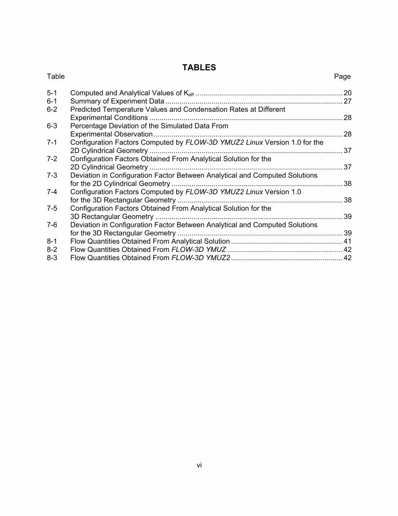
TABLES Table Page 5-1 Computed and Analytical Values of Keff .......................................................................... 20 6-1 Summary of Experiment Data ......................................................................................... 27 6-2 Predicted Temperature Values and Condensation Rates at Different Experimental Conditions ................................................................................................. 28 6-3 Percentage Deviation of the Simulated Data From Experimental Observation............................................................................................... 28 7-1 Configuration Factors Computed by FLOW-3D YMUZ2 Linux Version 1.0 for the 2D Cylindrical Geometry ................................................................................................. 37 7-2 Configuration Factors Obtained From Analytical Solution for the 2D Cylindrical Geometry ................................................................................................. 37 7-3 Deviation in Configuration Factor Between Analytical and Computed Solutions for the 2D Cylindrical Geometry ...................................................................................... 38 7-4 Configuration Factors Computed by FLOW-3D YMUZ2 Linux Version 1.0 for the 3D Rectangular Geometry ................................................................................... 38 7-5 Configuration Factors Obtained From Analytical Solution for the 3D Rectangular Geometry .............................................................................................. 39 7-6 Deviation in Configuration Factor Between Analytical and Computed Solutions for the 3D Rectangular Geometry ................................................................................... 39 8-1 Flow Quantities Obtained From Analytical Solution ........................................................ 41 8-2 Flow Quantities Obtained From FLOW-3D YMUZ .......................................................... 42 8-3 Flow Quantities Obtained From FLOW-3D YMUZ2 ........................................................ 42
1
1 INTRODUCTION This report documents the validation and installation test of the software FLOW-3D YMUZ2 Linux Version 1.0. The validation exercise of the code is performed through regression analysis. In the regression method a new validation test plan is not generated. Instead, the test plan and the test results that were used to validate the previous version of the software are adopted as a benchmark to assess the capability of the new version. A regression test is usually performed when software is updated to a newer version or is installed on a different platform. In essence it is a repetition of a previous validation study (i) to ensure that the software is performing in accordance with the required guidelines established in the original software validation test plan or (ii) to determine whether the software is producing results equivalent to those obtained from the previous version. A number of customized subroutines were written as an addendum to the standard commercial Navier-Stokes solver FLOW-3D® Version 9.0 to model the moisture transport inside the computational domain along with radiation heat transfer. The modified flow solver with enhanced capability was called FLOW-3D YMUZ2. The validation test plan and the validation report for FLOW-3D YMUZ2 are available in the reports of Green and Manepally (2006a, 2006b). The users manual for the solver FLOW-3D YMUZ2 (Das, et al. 2007) describes the procedure to use the code with the description of relevant input parameters that are illustrated with example inputs. Later the customized subroutines created for FLOW-3D YMUZ2 was adapted to the standard flow solver FLOW-3D Version 9.2 in the Linux operating system. No new capabilities or new customized subroutines were created. In this process the customized subroutines developed for FLOW-3D YMUZ2 were compiled using the Intel FORTRAN compiler in the Linux operating system and plugged onto the parent flow solver FLOW-3D Version 9.2. This flow solver is called FLOW-3D YMUZ2 Linux Version 1.0 and is identical to FLOW-3D YMUZ2 in terms of modeling capability of radiation heat transfer and moisture transport. No additional input parameters or logical switches are necessary in FLOW-3D YMUZ2 Linux. The basic difference between FLOW-3D YMUZ2 Linux Version 1.0 and FLOW-3D YMUZ2 are listed below.
1. FLOW-3D YMUZ2 Linux Version 1.0 is compiled on a multiprocessor machine in a Linux operating system, whereas FLOW-3D YMUZ2 was compiled in the Windows operating system. As a result, it is possible to run FLOW-3D YMUZ2 Linux Version 1.0 in parallel mode.
2. FLOW-3D YMUZ2 Linux Version 1.0 uses the flow solver FLOW-3D Version 9.2
as the baseline for compiling the additional modules, whereas FLOW-3D YMUZ2 used FLOW-3D Version 9.0 as the baseline solver. The baseline solvers FLOW-3D Versions 9.0 and 9.2 have some minor difference in modeling capabilities. These differences are documented in the users manual (Flow Science, Inc., 2007a) and the software release notice (Flow Science, Inc., 2007b) of Version 9.2. These differences, however, have no bearing on the moisture transport and radiation modules.
Because no new capabilities were added to the existing moisture transport and radiation modules, a new validation study for the solver FLOW-3D YMUZ2 Linux Version 1.0 is not necessary. A validation study through regression based on the previous validation

2
test plan is sufficient to assess the capability of the solver. A thorough regression analysis is carried out to study the effect of
1. Changing from Windows to the Linux operating system 2. Using the new baseline solver (Version 9.2)
In the regression analysis, the test cases used to validate the solver FLOW-3D YMUZ2 are simulated again using the new solver FLOW-3D YMUZ2 Linux, and the results are either compared with the experimental data or with previously validated simulation results. The results obtained from the solver FLOW-3D YMUZ2 Linux Version 1.0 are within the acceptable range. There are some minor differences in terms of modeling capabilities between FLOW-3D Version 9.0 and Version 9.2. These differences are assessed in the regression test. The input parameters are keywords for these two versions and are almost identical as the moisture transport module and radiation modules use their user-defined independent keywords; they are not affected by the change in nomenclature. This study is done to satisfy the quality assurance requirement of acquired and modified software as delineated in the procedure TOP-18. This chapter of the document describes the background of the flow solver and the necessity to perform this regression test. 1.1 Background FLOW-3D Version 9.2 (Flow Science, Inc., 2005) is a general purpose computational fluid dynamics (CFD) simulation software package founded on the algorithms for simulating fluid flow that were developed at Los Alamos National Laboratory in the 1960s and 1970s. It has been widely used to solve technical problems ranging from basic hydraulics to micro-electro-mechanical devices. FLOW-3D uses an ordered grid scheme that is oriented along a Cartesian or a polar-cylindrical coordinate system. Fluid flow and heat transfer boundary conditions are applied at the six orthogonal mesh limit surfaces. The code uses the so-called “Volume of Fluid” formulation Flow Science, Inc., pioneered to incorporate solid surfaces into the mesh structure and the computing equations. Three-dimensional solid objects are modeled as collections of blocked volumes and surfaces. This method retains the advantages of solving the difference equations on an orthogonal, structured grid The code implements a Boussinesq approach to modeling buoyant fluids in an otherwise incompressible flow regime. The Boussinesq approximation neglects the effect of fluid (air) density dependence on the pressure of the air phase, but includes the density dependence on temperature. Fluid turbulence is included in the simulation equations via a choice of turbulence models incorporated into the software. The user must choose whether fluid turbulence is significant and, if so, which turbulence model is appropriate for a particular simulation. The standard version of FLOW-3D, however, is not capable of modeling radiative heat transfer or moisture redistribution processes required to model the in-drift flow physics of the potential repository at Yucca Mountain. To effectively use the standard FLOW-3D
3
package for the numerical simulation of in-drift thermal and transport processes, new modules were developed to incorporate radiative heat transfer and moisture transport processes to specifically simulate the Yucca Mountain in-drift convection and heat transfer problem. The modified version of the FLOW-3D simulation package with these modules is called FLOW-3D YMUZ2 Version 1.0. The modified flow solver could be used as a tool to independently assess the approaches DOE is currently considering for calculating in-drift heat transfer and moisture redistribution in its performance assessment model. It could also be used to support, verify, and assess the near- field environment computations in the Total-system Performance Assessment (TPA) code. The FLOW-3D YMUZ2 flow solver could also be used to carry out parametric studies to develop insights for the uncertainties in the near-field environment and in-drift physical processes. The radiation and moisture transport modules were developed based on the flow solver FLOW-3D Version 9.0 in Microsoft ® Windows® operating system. The developed modules were later ported in the Linux operating system on the solver FLOW-3D Version 9.2 The users manual for the solver FLOW-3D YMUZ2 (Das, et al. 2007) details the Moisture Transport and Radiation Modules and the relevant input files, parameters necessary to use these modules, example problems, and installation procedures. The manual also delineates the theory used to model the radiation and moisture transport processes, followed by brief guidelines to program the modules using standard FORTRAN 77 language. The input parameters necessary for FLOW-3D YMUZ2 Linux Version 1.0 are the same as those in FLOW-3D YMUZ2 for the moisture transport and radiation modules. The example problems described in the users manual could also be used for FLOW-3D YMUZ2 Linux. The installation procedure for FLOW-3D YMUZ2 Linux Version 1.0 is different from FLOW-3D YMUZ2 due to a change in the operating system, and the new procedure is described in this document. 1.2 Scope of Regression Tests The regression study is restricted to the following four sets of test cases.
• Natural convection • Moisture transport • Radiation heat transfer • Combined moisture transport and radiation heat transfer
The original validation study was performed on these test cases, and the regression study repeats those tests and compares the results with either existing simulation data available from the validation study or with the experimental data. These four categories cover the broad technical area where the code is expected to be used at the Center for Nuclear Waste Regulatory Analyses (CNWRA®). Details of each of the test cases and expected results are discussed in the original software validation test plan (Green and Manepally 2006a) and validation report (Green, 2006). In this report, the details of the test procedure are not discussed; only the relevant results are shown with comments on the acceptability of the results.

4
2 ENVIRONMENT
2.1 Hardware Requirements The baseline program can be run on computers with Windows or Linux/UNIX operating systems as described in the FLOW-3D Version 9.2 manual. The FLOW-3D YMUZ2 Linux Version 1.0 was, however, built on the Redhat Linux operating system. All of the tests described here were conducted on the cluster Katana at CNWRA. The Intel FORTRAN compiler was used to build the executables. The present build of FLOW-3D YMUZ2 Linux Version 1.0 used Open-MP-based parallelization that uses multiple processor shared memory machines. The current configuration of the cluster katana allows parallelization using four processes. 2.2 Software for the Baseline Flow Solver The FLOW-3D software package has been in use since the early 1980s. It was originally based on algorithms the founders of Flow Science, Inc., developed when they were employed at Los Alamos National Laboratory. While the original code was a general purpose CFD package that could simulate the effects of irregular solid objects, it was especially noted for its ability to simulate free surfaces and reduced gravity. The current version of the code is a much-enhanced descendent of that early software package and is widely used in industry and government agencies. A description of the software may be found at the Flow Science, Inc. website (Flow Science, Inc. 2008) The baseline solver FLOW-3D Version 9.2 for the present tests is used in a Linux operating system. The baseline solver is precompiled by Flow Science, Inc. using the Intel FORTRAN compiler, and the required modules needed to link the customized routines are provided with the standard build. The solver is capable of performing parallel computing using a multiple processor shared memory system. 2.3 Installation of FLOW-3D YMUZ2 Linux The installation process follows. However, this process is only needed for a new build when there is a code change. The standard process could be to copy the executable available in the CD and set the environment variables. The process of setting the path and environment variables are described in subsequent sections.
1. Copy the contents of the directory with all the flow3d executables in a secure location in your home area ($cp –r /opt/flow3d/* /export/home/kaushik/flow3dtest/)
2. Change directory to the secure location where you want to test the installation ($cd /export/home/kaushik/flow3dtest)
3. Backup the flow3d existing source file by copying it in backup area $mkdir source-backup
a. $cd source b. $mv * ../source-backup/ c. $cd .. d. $rm -rf source
4. Copy the contents of the flow3dymuz2 source code in the test directory (using some of the effect $cp –r source/ /export/home/kaushik/flow3dtest)

5
5. Run make clean from the test directory ($ cd /export/home/kaushik/flow3dtest; $ make clean)
6. Copy the pcg_rad_module.mod in different required directories. From the source/comdek directory, select
a. cp pcg_rad_module.mod ../../prehyd/prep3d/ b. cp pcg_rad_module.mod ../../prehyd/hydr3d/ c. cp pcg_rad_module.mod ../../prehyd/utility/ d. cp pcg_rad_module.o ../../prehyd/prep3d/ e. cp pcg_rad_module.o ../../prehyd/hydr3d/ f. cp pcg_rad_module.o ../../prehyd/utility/ Note that the pcg_rad_module.mod module is compiled using the Intel Fortran 90 64-bit version compiler in the Linux operating system. If the compiler changes, it needs to be recompiled to create the module and object files using the following commands:
a. ifort (or whatever fortran 90 compiler is there) pcg_rad_module.f b. ifort –c pcg_rad_module.f (to create the object file that will be needed
later)
7. Perhaps the most important part of the installation is altering the libraries. This should be done with utmost care as any change will seriously affect the code and mistakes will cause erroneous results. The steps follow
i. In the test directory, go to prehyd/hydr3d and execute the following:
1. ar -vd binlib.a qsadd.o 2. ar -vd binlib.a rusrd.o 3. ar -vq binlib.a pcg_rad_module.o
ii. In the test directory, go to prehyd/utility and execute the following 1. cp ~/”test-directrory”/source/hydra3d/teval_stg.o ~/”test-
directrory”/prehyd/utility/ 2. ar -vd utilib.a e1cal.o 3. ar -vd utilib.a rhocal.o 4. ar -vd utilib.a teval.o 5. ar -vq utilib.a teval_stg.o
iii. In the test directory, go to prehyd/prep3d and execute the following
1. ar -vd binlib.a prusrd.o 8. Return to the main directory and type make
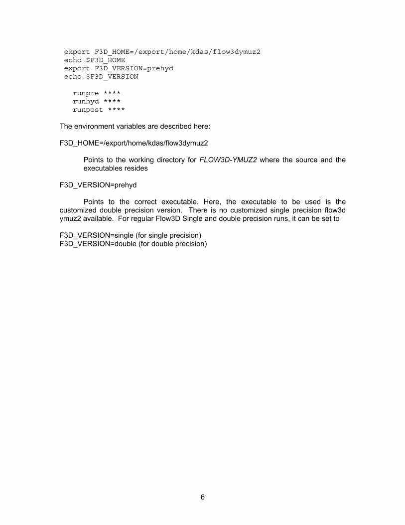
2.4 Running FLOW-3D YMUZ2 Linux Version 1.0 in Parallel Environment The run script will be similar to the following example. #! /bin/bash echo Date and time is `date` export omp_num_threads=4 echo $omp_num_threads
6
export F3D_HOME=/export/home/kdas/flow3dymuz2 echo $F3D_HOME export F3D_VERSION=prehyd echo $F3D_VERSION runpre **** runhyd **** runpost **** The environment variables are described here: F3D_HOME=/export/home/kdas/flow3dymuz2
Points to the working directory for FLOW3D-YMUZ2 where the source and the executables resides
F3D_VERSION=prehyd Points to the correct executable. Here, the executable to be used is the customized double precision version. There is no customized single precision flow3d ymuz2 available. For regular Flow3D Single and double precision runs, it can be set to F3D_VERSION=single (for single precision) F3D_VERSION=double (for double precision)

7
3 PREREQUISITES Users should be trained to use FLOW-3D and have experience in fluid mechanics and heat transfer.
4 ASSUMPTIONS AND CONSTRAINTS None.
5 NATURAL AND FORCED CONVECTION The regression test cases described in this section validate the FLOW-3D YMUZ2 Linux Version 1.0 code for application in natural and forced convection. All the test cases are detailed in the validation report (Green, 2006) of FLOW3D-YMUZ2. 5.1 Laminar Natural Convection on a Vertical Surface The analytical solution Incropera and Dewitt (1996) documented is used for validation purposes. The empirical correlation in Churchill and Chu (1975) provides an improvement to the analytical solution for average Nusselt number at lower Rayleigh numbers. The physics of the flow and related test matrix is described in Green (2006). 5.1.1 Test Input The test input used for the regression test is identical to that used in the validation study of FLOW-3D YMUZ2. The model was developed with an isothermal vertical wall with a temperature of 340 K [152EF] (Green 2006). The computational domain is shown in Figure 5-1. In the original validation study, a number of grids were used to perform the mesh refinement study. In the present test, only the fine mesh simulations were performed. The input, output, and the postprocessed data are provided in the attached media in the directory \no-moisture-no-radiation\Laminar-vertical-plate. 5.1.2 Expected Test Results The test result obtained from FLOW-3D YMUZ2 Linux Version 1.0 is expected to be almost identical to that obtained by FLOW-3D YMUZ2 and be within 10percent bound of the analytical solution. 5.1.3 Test Results The overall flowfield obtained from FLOW-3D YMUZ2 and FLOW-3D YMUZ2 Linux Version 1.0 is shown in Figure 5-2. The results qualitatively match each other and appear to be identical.

8
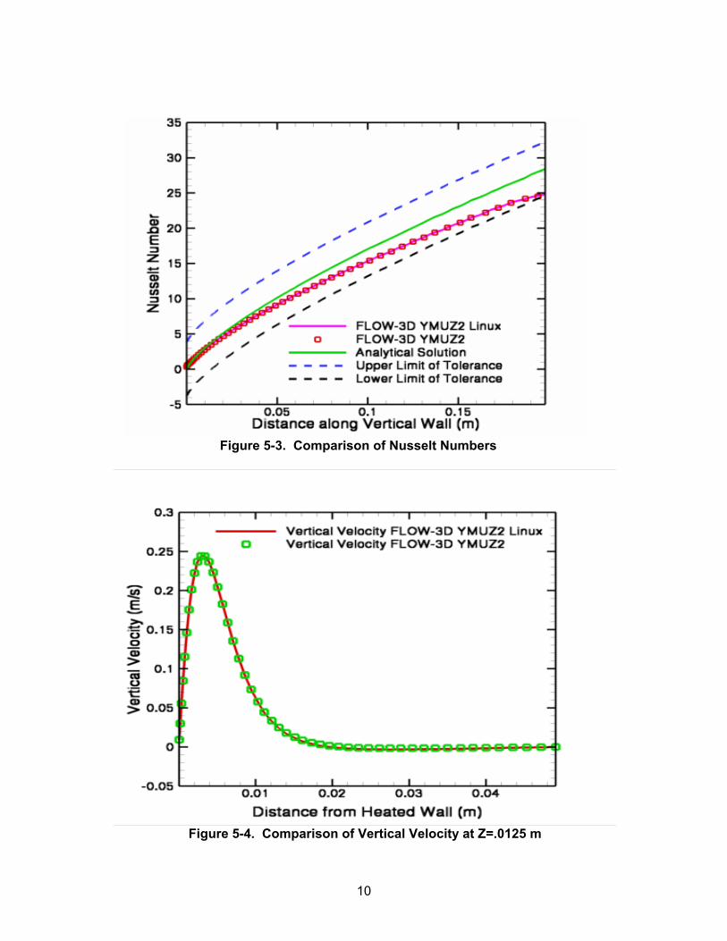
The FLOW-3D YMUZ2 Linux Version 1.0 predictions are compared to those obtained from the analytical expression and FLOW-3D YMUZ2 in Figure 5-3. The local Nusselt number results for the nominal mesh were within "10 percent of the analytical solution. These variances are within the acceptance criteria described above; it can also be observed that the solvers FLOW-3D YMUZ2 Linux Version 1.0 and FLOW-3D YMUZ2 provide almost identical trend. The variation between the results is less than 0.001 percent.
Figure 5-1. Computational Domain for Vertical Flat Plate Test Case

9
(a) (b) Figure 5-2. Velocity Vectors and Temperature Contours for (a) FLOW-3D YMUZ2 Linux
Version 1.0 and (b) FLOW-3D YMUZ2
10
Figure 5-3. Comparison of Nusselt Numbers
Figure 5-4. Comparison of Vertical Velocity at Z=.0125 m

11
Figure 5-5. Comparison of Temperature at Z=.0125 m
The vertical velocity profiles obtained from FLOW-3D YMUZ2 Linux Version 1.0 and FLOW-3D YMUZ2 at a height of vertical velocity at Z =.0125 m are compared in Figure 6-4 which shows that the results have identical trend. In Figure 6-5, the horizontal temperature distribution at the same location obtained from both the solvers is compared; they match exactly, confirming the previous observation that they produce an identical result. 5.2 Turbulent Natural Convection in an Air-Filled Square Cavity An experimental study Ampofo and Karayiannis (2003) conducted is used to test the accuracy of FLOW-3D YMUZ2 Linux Version 1.0 for natural convection in low-level turbulence. The physics of the flow and related test matrix is described in Green (2006). 5.2.1 Test Input The test input used for the regression test is identical to that used in the validation study of FLOW-3D YMUZ2. The experiment was modeled as two-dimensional with an incompressible fluid and the Boussinesq approximation to capture the thermal buoyancy effects. The large eddy simulation model in FLOW-3D was used to model the fluid turbulence and capture the corner vortices. The computational domain is shown in Figure 5.1.
12
The input, output, and the postprocessed data are provided in the attached media in the directory\no-moisture-no-radiation\Laminar-vertical-plate. 5.2.2 Expected Test Results The test result obtained from FLOW-3D YMUZ2 Linux Version 1.0 is expected to be almost identical to that obtained by FLOW-3D YMUZ2 and to be within 10 percent bound of the analytical solution. The criteria for test acceptance were established in the software validation test plan (Green and Manepally, 2006a), and the results are presented in the validation report (Green 2006). In the original validation study, a number of grids were used to perform the mesh refinement study. In the present test, only the fine mesh simulations were performed. 5.2.3 Test Results The overall flowfield obtained from FLOW-3D YMUZ2 and FLOW-3D YMUZ2 Linux Version 1.0 is shown in Figure 5-2. The results qualitatively match each other and appear to be identical. It is not possible, however, to produce an exact match, as Large Eddy Simulators are being used to compute the turbulent quantities that produce time-dependent quantities rather than averaged steady values. The local Nusselt number distribution along the hot vertical wall and the upper wall is shown in Figures 5-3 and 5-4. The computed values obtained from FLOW-3D YMUZ2 Linux Version 1.0 and FLOW-3D YMUZ2 match well with each other. There is some minor variation in the Nusselt number values along the vertical wall, which is an artifact of the unsteadiness in the flowfield. These results are presented for an instantaneous snapshot instead of time-averaged quantities, which cause localized minor deviation. Dimensionless temperature variation along the mid-width and mid-height of the domain are presented in Figures 5-5 and 5-6. Both the flow solvers produce identical results, with variation less than 1 percent at certain locations. Figure 5-7 shows a comparison of velocity distribution at mid-height of the domain for the solvers FLOW-3D YMUZ2 Linux Version 1.0 and FLOW-3D YMUZ2. They produce almost an identical pattern, confirming that the newly built solver can correctly model natural convection flows.

13
Figure 5-6. Domain of Solution for Natural Convection in a Square Cavity

14
Figure 5-7. Predicted Fluid Temperature and Velocity Vectors (a) Using FLOW-3D YMUZ2 and (b) FLOW-3D YMUZ2 Linux
(a) (b)
0
20
40
60
80
100
120
0.00E+00 2.00E-01 4.00E-01 6.00E-01 8.00E-01 1.00E+00
Dimensionless Distance from Bottom Wall
Loca
l Nus
selt
Num
ber
FLOW-3D YMUZ2 LinuxFLOW-3D YMUZ2
Figure 5-8. Comparison of Local Nusselt Number Along the Hot Vertical Wall

15
-30
-20
-10
0
10
20
30
40
50
60
0.00E+00 2.00E-01 4.00E-01 6.00E-01 8.00E-01 1.00E+00 1.20E+00
Dimensionless Distance along Hot Wall
Loca
l Nus
selt
Num
ber
FLOW-3D YMUZ2 LinuxFLOW-3D YMUZ2
Figure 5-9. Comparison of Local Nusselt Number Along the Top Wall
-0.1
0.1
0.3
0.5
0.7
0.9
0.00E+00 2.00E-01 4.00E-01 6.00E-01 8.00E-01 1.00E+00 1.20E+00
Dimensionless Distance from Bottom Wall (x/L=0.5)
Dim
ensi
onle
ss T
empe
ratu
re
FLOW-3D YMUZ2 LinuxFLOW-3D YMUZ2
Figure 5-10. Comparison of Dimensionless Temperature at the Mid-Width (x/L=0.5)

16
0
0.1
0.2
0.3
0.4
0.5
0.6
0.7
0.8
0.9
0.00E+00 2.00E-01 4.00E-01 6.00E-01 8.00E-01 1.00E+00 1.20E+00
Dimensionless Distance from Hot Wall (y/L=0.5)
Dim
ensi
onle
ss T
empe
ratu
re
FLOW-3D YMUZ2 LinuxFLOW-3D YMUZ2
Figure 5-11. Comparison of Dimensionless Temperature Distribution at Mid-Height (y/L=0.5)
-0.4000
-0.3000
-0.2000
-0.1000
0.0000
0.1000
0.2000
0.3000
0.00E+00 2.00E-01 4.00E-01 6.00E-01 8.00E-01 1.00E+00 1.20E+00
Dimensionless Distance from Hot Wall (y/L)=0.5
Vert
ical
VEl
ocity
(m/s
)
FLOW-3D YMUZ2 LinuxFLOW-3D YMUZ2
Figure 5-12. Comparison of Velocity Distribution at Mid-Height (y/L=0.5)

17
5.3 Natural Convection in an Annulus Between Horizontal Concentric Cylinders Kuehn and Goldstein (1978) conducted detailed experiments on the thermal behavior of a gas in an annulus between concentric and eccentric circular cylinders. They presented results in terms of temperature distribution and effective thermal conductivity, which is widely used as a benchmark to validate the computational fluid dynamic solvers. The physics of the flow and the equations to determine the effective thermal conductivity for this test are detailed in the original paper of Kuehn and Goldstein (1978), and the relevant equations are documented in the software validation report of Green (2006). 5.3.1 Test Input The test input used for the regression test is identical to that used in the validation study of FLOW-3D YMUZ2. However, in the original test case, different flow conditions covering the laminar, transitional, and turbulent flow regimes and that are represented by different Rayleigh numbers were simulated to test the effectiveness of the solver. FLOW-3D input files were developed for the cases for RaL = 1.31 × 10³, RaL = 6.19 × 10⁴, RaL = 6.81 × 10⁵, RaL = 2.51 × 10⁶, RaL = 1.90 × 10⁷, and RaL = 6.60 × 10⁷. In the present investigation, only one Rayleigh number (6.8 × 10⁵) is considered. This Rayleigh number represents turbulent flow, and an effective simulation could be considered sufficient for the purposes of the regression test. The computational domain is shown in Figure 5-6. In the original validation study, a number of grids were used to perform the mesh refinement study. In the present test, only the fine mesh simulations were performed. The input, output, and the postprocessed data are provided in the attached media in the directory\no-moisture-no-radiation\Kuehn and Goldstein. 5.3.2 Expected Test Results The criteria for test acceptance were established in the software validation test plan (Green and Manepally, 2006a). The acceptance criterion was stated to be the overall equivalent thermal conductivity with a deviation of no more than 25 percent of the measured value. The test result obtained from FLOW-3D YMUZ2 Linux Version 1.0 is expected to be almost identical to that obtained by FLOW-3D YMUZ2, and the overall flowfield should have a qualitative resemblance. In addition, the effective thermal conductivity values obtained from FLOW-3D YMUZ2 Linux Version 1.0 should be within accepted limits as prescribed in the validation test plan (Green, 2006) as well as within one percent within the value prescribed by FLOW-3D YMUZ2. 5.3.3 Test Results The overall flowfield obtained from FLOW-3D YMUZ2 and FLOW-3D YMUZ2 Linux Version 1.0 is shown in Figure 5-7. The results qualitatively match each other and appear to be identical.

18
Figure 5-13. Schematic of the Problem of Natural Convection Between Two
Concentric Cylinders Table 5-1 compares the value of effective thermal conductivity obtained from FLOW-3D YMUZ2 and FLOW-3D YMUZ2 Linux Version 1.0 with the analytical solution. The deviation of the Keff value calculated by FLOW-3D YMUZ2 Linux Version 1.0 is less than 10 percent from the analytical solution, and the difference between the computed value of Keff using FLOW-3D YMUZ2 and FLOW-3D YMUZ2 Linux Version 1.0 is less than 1 percent.
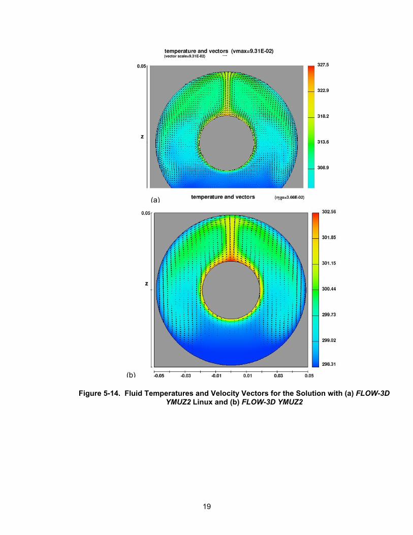
19
Figure 5-14. Fluid Temperatures and Velocity Vectors for the Solution with (a) FLOW-3D YMUZ2 Linux and (b) FLOW-3D YMUZ2
(a)
(b)

20
Table 5-1 Computed and Analytical Values of Keff Variable Value
Raleigh Number 6.8×10⁵ Keq FLOW-3D YMUZ2 Linux Version 1.0
(W/m-K) 5.28
Keq FLOW-3D YMUZ2 (W/m-K) 5.27 Keq Analytical Solution (W/m-K) 5.60
Percent deviation from analytical solution -5.66 Percent deviation from FLOW-3D YMUZ2 -0.2
5.4 Natural Convection Inside a Ventilated Heated Enclosure Test Case 4 will compare FLOW-3D results against measured data from a natural ventilation experiment (Dubovsky, et al., 2001). This test case also compares the data with a different numerical model created in FLUENT 4.52 (Fluent Inc., 1994). However, the original input and output files from the previous simulations could not be tracked and this test case was not repeated for regression analysis. This test, however, is not critical to establish that the solvers FLOW3D-YMUZ2 Linux and FLOW-3D YMUZ2 have the same functionality and provide analogous results because
a. The previous three tests already prove that FLOW3D-YMUZ2 Linux is capable of simulating natural convection and the predicted flowfield is identical to that produced by FLOW3D-YMUZ2. Additional tests will just reestablish it.
b. None of the test cases described in this chapter deal with moisture
transport and radiation heat transfer or use the standard solver. The test cases described in this chapter fundamentally validate the baseline flow solver. Flow Science, Inc. has an established test case database for the standard solver FLOW-3D Versions 9.0 and 9, which extensively document the validation exercise. Additional tests are not required to validate the standard solver.
21
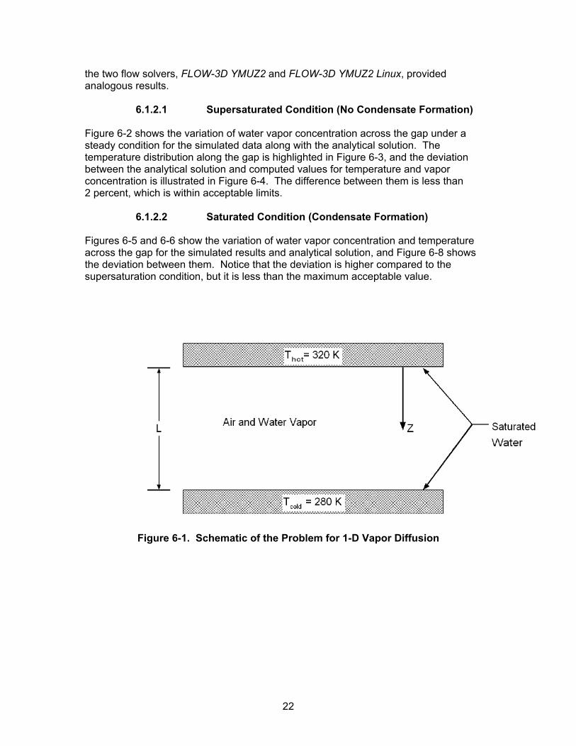
6 MOISTURE TRANSPORT TEST CASES The regression test cases described in this section are meant to revalidate the moisture transport module of the flow solver FLOW-3D YMUZ2 Linux Version 1.0 in predicting the diffusion of water in an air/water mixture, the advection transport of water in a natural convection flow, and the phase change processes that are inherent under these conditions. 6.1 Conduction Heat Transfer and Vapor Diffusion This hypothetical test case is formulated to simulate moisture transport through a gap that is limited by two flat plates at two different temperatures. This test case is depicted schematically in Figure 6-1. The following parameters define the necessary geometric and physical properties of the system (Green, 2006): • Gap thickness, L = 0.1 m [0.33 ft] • Fluid thermal conductivity = kmix = 0.026 W/(m 2-K) [0.005 BTU/h-ft 2-°F] • Top (hot) surface temperature = Th = 320 K [116°F] • Bottom (cold) surface temperature = Tc = 280 K [44.3°F] • Pressure = 1 atm The input, output, and the postprocessed data are provided in the attached media in the directory \moist and rad\1-D_Diffusion_Ver_Test. 6.1.1 Expected Test Results Bird, et al. (1960) describes the equation for diffusive moisture flow. The Green (2006) software validation report provides the analytical solution for the equations under two different operating conditions: (a) The relative humidity in the domain is not restricted to 100 percent; as a result, no
condensate is formed. (b) The relative humidity is restricted to 100 percent and condensate forms in the
domain. The regression test is performed for both the test cases. A FLOW-3D input file was developed to model the idealized case of one-dimensional conduction heat transfer and chemical species diffusion through the air gaps. The original input files from the validation studies are used for the regression test. The test result obtained from FLOW-3D YMUZ2 Linux Version 1.0 is expected to be almost identical to that obtained by FLOW-3D YMUZ2 and be within 10 percent bound of the analytical solution. 6.1.2 Test Results The temperature and vapor concentration along the gap for two test cases are plotted along with the analytical solution for comparison. Also, the deviation in the predicted and analytical results is shown to obtain a quantitative estimate of error. In this test case, the FLOW-3D YMUZ2 and FLOW-3D YMUZ2 Linux Version 1.0 results are not plotted simultaneously. A comparison of the results obtained from FLOW-3D YMUZ2 Linux Version 1.0 with analytical solution is sufficient to gain confidence in the solver, and the result for the same test case in the validation exercise (Green 2006) shows that
22
the two flow solvers, FLOW-3D YMUZ2 and FLOW-3D YMUZ2 Linux, provided analogous results.
6.1.2.1 Supersaturated Condition (No Condensate Formation) Figure 6-2 shows the variation of water vapor concentration across the gap under a steady condition for the simulated data along with the analytical solution. The temperature distribution along the gap is highlighted in Figure 6-3, and the deviation between the analytical solution and computed values for temperature and vapor concentration is illustrated in Figure 6-4. The difference between them is less than 2 percent, which is within acceptable limits.
6.1.2.2 Saturated Condition (Condensate Formation) Figures 6-5 and 6-6 show the variation of water vapor concentration and temperature across the gap for the simulated results and analytical solution, and Figure 6-8 shows the deviation between them. Notice that the deviation is higher compared to the supersaturation condition, but it is less than the maximum acceptable value.
Figure 6-1. Schematic of the Problem for 1-D Vapor Diffusion

23
0
0.02
0.04
0.06
0.08
0.1
0.12
0 0.05 0.1 0.15 0.2
Distance from Hot End m
Vapo
r con
cent
ratio
n (m
ol %
) 1-D TheoryFLOW-3D Results
No Fog Allow ed
Figure 6-2. Spatial Variation of Vapor Concentration Using FLOW-3D YMUZ2 Linux
Version 1.0 for Supersaturated Air
Figure 6-3. Spatial Variation of Temperature Using FLOW-3D YMUZ2 Linux Version 1.0 for Supersaturated Air
275280
285290
295300305
310315
320325
0 0.05 0.1 0.15 0.2
Distance from Hot End m
Tem
pera
ture
K
1-D TheoryFLOW-3D Results
No Fog Allowed

24
Figure 6-4. Deviation in Temperature and Concentration Using FLOW-3D YMUZ2 Linux
Version 1.0 for Supersaturated Air
Figure 6-5. Spatial Variation of Vapor Concentration Using FLOW-3D YMUZ2 Linux Version 1.0 for Saturated Air
-2.5%
-2.0%
-1.5%
-1.0%
-0.5%
0.0%
0.5%
1.0%
1.5%
2.0%
0 0.05 0.1 0.15 0.2
Distance from Hot End
Dev
iatio
n %
TemperatureVapor Concentration
No Fog Allow ed
0
0.02
0.04
0.06
0.08
0.1
0.12
0 0.05 0.1 0.15 0.2
Distance from Hot End m
Vapo
r con
cent
ratio
n (m
ol %
) 1-D TheoryFLOW-3D Results
Fog Allowed

25
-5%
-4%
-3%
-2%
-1%
0%
1%
2%
3%
4%
0 0.05 0.1 0.15 0.2
Distance from Hot End
Dev
iatio
n %
TemperatureVapor Concentration
Fog Allow ed
Figure 6-7. Deviation in Temperature and Concentration Using FLOW-3D YMUZ2 Linux for Saturated Air
275280
285290
295300305
310315
320325
0 0.05 0.1 0.15 0.2
Distance from Hot End m
Tem
pera
ture
K1-D TheoryFLOW -3D Results
Fog A llow ed
Figure 6-6. Spatial Variation of Temperature Using FLOW-3D YMUZ2 Linux for Saturated Air
26
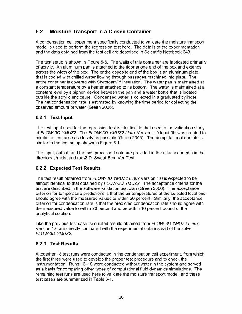
6.2 Moisture Transport in a Closed Container A condensation cell experiment specifically conducted to validate the moisture transport model is used to perform the regression test here. The details of the experimentation and the data obtained from the test cell are described in Scientific Notebook 643. The test setup is shown in Figure 5-6. The walls of this container are fabricated primarily of acrylic. An aluminum pan is attached to the floor at one end of the box and extends across the width of the box. The entire opposite end of the box is an aluminum plate that is cooled with chilled water flowing through passages machined into plate. The entire container is covered with Styrofoam™ insulation. The water pan is maintained at a constant temperature by a heater attached to its bottom. The water is maintained at a constant level by a siphon device between the pan and a water bottle that is located outside the acrylic enclosure. Condensed water is collected in a graduated cylinder. The net condensation rate is estimated by knowing the time period for collecting the observed amount of water (Green 2006). 6.2.1 Test Input The test input used for the regression test is identical to that used in the validation study of FLOW-3D YMUZ2. The FLOW-3D YMUZ2 Linux Version 1.0 input file was created to mimic the test case as closely as possible (Green 2006). The computational domain is similar to the test setup shown in Figure 6.1. The input, output, and the postprocessed data are provided in the attached media in the directory \ \moist and rad\2-D_Sweat-Box_Ver-Test. 6.2.2 Expected Test Results The test result obtained from FLOW-3D YMUZ2 Linux Version 1.0 is expected to be almost identical to that obtained by FLOW-3D YMUZ2. The acceptance criteria for the test are described in the software validation test plan (Green 2006). The acceptance criterion for temperature predictions is that the air temperatures at the selected locations should agree with the measured values to within 20 percent. Similarly, the acceptance criterion for condensation rate is that the predicted condensation rate should agree with the measured value to within 20 percent and be within 10 percent bound of the analytical solution. Like the previous test case, simulated results obtained from FLOW-3D YMUZ2 Linux Version 1.0 are directly compared with the experimental data instead of the solver FLOW-3D YMUZ2. 6.2.3 Test Results Altogether 18 test runs were conducted in the condensation cell experiment, from which the first three were used to develop the proper test procedure and to check the instrumentation. Runs 16–18 were conducted without water in the system and served as a basis for comparing other types of computational fluid dynamics simulations. The remaining test runs are used here to validate the moisture transport model, and these test cases are summarized in Table 6-1.

27
Table 6-1. Summary of Experiment Data
Condensation Rate (ml/hr)
Water Temp.
(C )
Cold Plate
Temp. (C )
Air Temp. Lower
(C )
Air Temp. Middle
(C)
Air Temp. Upper
(C )
Temp. Top
Chamber (C )
Temp. Top
Insulation (C )
Ambient Temp (C )
Water Cold Plate T (C )
1 8.8 38.6 10.7 22.9 26.0 27.2 25.4 23.7 23.6 28.0 2 16.8 46.1 10.8 26.6 30.2 31.5 29.0 24.1 23.4 35.3 3 25.6 54.3 10.9 30.9 35.2 36.3 33.1 24.5 23.2 43.4 8 2.5 19.5 5.2 14.3 16.3 17.4 18.2 24.2 24.9 14.3 7 4.7 25.3 5.2 15.6 17.9 19.2 18.7 23.3 23.7 20.1 4 7.2 32.3 5.3 18.8 21.6 23.2 22.4 24.5 24.7 27.0 5 12.1 39.4 5.4 21.5 24.9 26.6 24.7 23.1 23.1 34.1 6 20.9 47.7 5.5 25.1 29.1 30.9 29.0 23.7 23.1 42.2 9 1.7 26.2 19.1 22.6 23.5 24.1 24.0 25.4 25.6 7.1 10 6.6 38.2 19.1 26.3 28.3 29.5 27.9 25.1 24.8 19.1 12 12.8 45.0 19.2 29.2 32.1 33.4 31.5 26.2 25.6 25.8 11 20.8 50.9 19.3 32.1 35.3 36.8 34.4 25.1 23.9 31.6 15 0.5 34.0 29.4 29.7 30.1 30.5 29.6 25.2 24.3 4.6 14 4.2 39.7 29.4 31.3 32.2 33.1 31.5 23.9 23.0 10.3 13 8.1 46.1 29.5 33.7 35.5 36.6 34.8 25.1 23.9 16.6 16 0.0 57.5 19.3 32.3 35.8 37.4 33.6 25.8 24.8 38.2 17 0.0 44.2 19.3 27.9 30.3 31.6 29.3 25.3 24.9 24.9 18 0.0 32.3 19.2 23.8 25.2 26.1 25.0 23.8 23.4 13.1
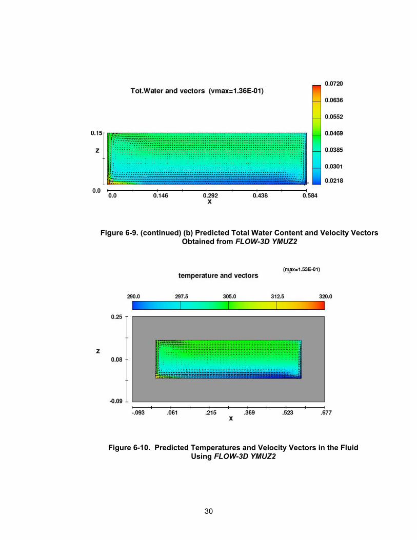
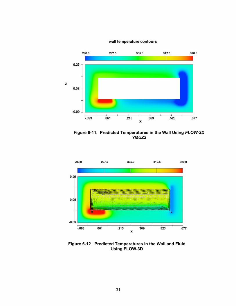
Velocity vectors and total water content contours obtained from the simulated results using FLOW-3D YMUZ2 Linux Version 1.0 and FLOW-3D YMUZ2 are shown in Figure 6-9 (a) which shows that the flowfield predicted by these two solvers is similar. Figures 6-10 through 6-11 show the predicted temperature contours in the flowfield and the wall for FLOW-3D YMUZ2 Linux Version 1.0 and FLOW-3D YMUZ2. These plots reaffirm that the results generated by these two solvers are analogous. The temperatures at three different points (shown in Figure 6-8) are plotted for different test conditions in Figure 6-13. The solid lines in the plot represent the computed data, whereas the symbols represent measured values. The difference between the measured values and the computed data is within the acceptable range as discussed next. Figure 6-14 shows the rate of condensation for the computed and experimental values at different experimental conditions, and the deviation between them is within the acceptable limit. Tables 6-2 and 6-3 present these results in a tabular form. Table 6-2 shows the predicted temperature values and the condensation rates at different experimental conditions. Table 6-3 shows the percentage deviation of the simulated data from experimental observation. The maximum deviation of computed data is less than 20 percent, which shows that the results from FLOW-3D YMUZ2 Linux Version 1.0 are acceptable.

28
Table 6-2. Predicted Temperature Values and Condensation Rates at Different Experimental Conditions
Condensation Rate (ml/hr)
Air Temp. Lower (C )
Air Temp. Middle (C )
Air Temp. Upper (C ) Max ΔT
-273.15 -273.15 -273.15 -273.15 -273.15 -273.15 -273.15 -273.15 -273.15
2.4 12.7 15.5 17.7 14.3 5.3 12.6 16.5 18.2 20.1 8.5 14.6 20.1 21.8 27.0
13.1 17.4 24.3 26.2 34.1 21.1 21.4 29.9 31.9 42.2 1.7 22.4 23.7 24.6 7.1 8.2 24.9 28.6 29.6 19.1
14.3 27.3 32.5 33.8 25.8 21.6 29.9 36.3 37.8 31.6 0.9 30.2 31.0 31.1 4.6 4.2 31.9 33.8 34.3 10.3 9.8 33.9 37.1 38.0 16.6
-273.15 -273.15 -273.15 -273.15 -273.15 -273.15 -273.15 -273.15 -273.15
Table 6-3. Percentage Deviation of the Simulated Data From Experimental Observation Condensation Rate Air Temp. Lower Air Temp. Middle Air Temp. Upper
-1.5% -11.3% -5.5% 2.0% 6.6% -14.9% -7.1% -4.6%
15.2% -15.4% -5.7% -5.2% 12.2% -12.2% -1.8% -1.2% 2.4% -8.9% 1.8% 2.2% 0.5% -2.4% 3.1% 6.4%
18.5% -7.4% 1.4% 0.5% 18.0% -7.5% 1.6% 1.7% 10.0% -7.1% 3.1% 3.2% 5.1% 10.9% 19.9% 13.9% 0.1% 6.0% 15.6% 11.8%
19.8% 0.8% 9.8% 8.3%

29
Figure 6-8. Test Setup for the Condensation Test Case
Figure 6-9. (a) Predicted Total Water Content and Velocity Vectors Obtained From
FLOW-3D YMUZ2 Linux
30
Figure 6-9. (continued) (b) Predicted Total Water Content and Velocity Vectors Obtained from FLOW-3D YMUZ2
Figure 6-10. Predicted Temperatures and Velocity Vectors in the Fluid Using FLOW-3D YMUZ2
31
Figure 6-11. Predicted Temperatures in the Wall Using FLOW-3D YMUZ2
Figure 6-12. Predicted Temperatures in the Wall and Fluid Using FLOW-3D

32
0
5
10
15
20
25
0 10 20 30 40 50
ΔT (Hot Water - Cold Plate) °C
Cond
ensa
tion
Rat
e m
L/hr
5.3°C Cold Plate19.2°C Cold Plate29.4°C Cold Plate
Symbols - MeasuredLines - Predictions
Figure 6-14. Cold Plate Condensation Rate Using FLOW-3D YMUZ2
0
5
10
15
20
25
30
35
40
0 10 20 30 40
ΔT (Hot Water - Cold Plate) °C
Tem
pera
ture
°C
Lower Air Mid-PlaneMiddle Air Mid-PlaneUpper Air Mid-Plane
Figure 6-13. Mid-line Temperature of the Ion Condensation Cell Using FLOW-3D YMUZ2

33
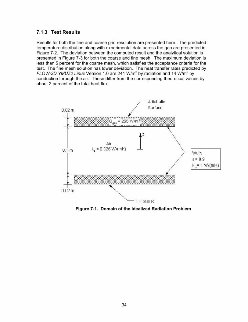
7 THERMAL RADIATION TEST CASES Two test cases related to radiation heat transfer are discussed in this section. The first test case tests the capability of FLOW-3D YMUZ2 Linux Version 1.0 to compute radiation heat transfer, and the second test case validates the capabilities of the radiation module in computing radiation configuration factors. These test cases are repeat tests of the validation study performed in connection to FLOW-3D YMUZ2. 7.1 Thermal Conduction and Radiation Between Two Surfaces Incropera and Dewitt (1996) documented the analytical solution used for the validation purpose. The physics of the problem and related test matrix are described in Green (2006). The test case described here is similar to that discussed in connection with one-dimensional diffusion. 7.1.1 Test Input The test input used for the regression test is identical to that used in the validation study of FLOW-3D YMUZ2. The computational domain is shown in Figure 7-1. The following parameters define the necessary geometric and physical properties of the system: • Gap thickness, tgap = 0.1 m [0.3 ft] • Plate thickness, tupper = tlower = 0.02 m [0.06 ft] • Emissivity, gupper = glower = 0.9 • Gap thermal conductivity = kair = 0.1 W/(m2-K) [0.0176 BTU/h-ft2-EF] • Plate thermal conductivity, kupper = klower = 1 W/(m2-K) [0.0176 BTU/h-ft2-EF] • Upper surface heat flux = Qupper = 255 W/m2 [80.8 BTU/h-ft2] • Temperature of outside surface of lower plate = Tc = 300 K [80.3 EF] The input, output, and the postprocessed data are provided in the attached media in the directory \moist and rad\1-D Radiation. Two sets of grids were used in the solution to study the effect of grid refinement. Both these grids produced identical results. An input file was developed to model the idealized case of one-dimensional conduction heat transfer through the three objects and closely mimic the idealized model. Air movement was disallowed in the simulation. Because this is an idealized one-dimensional case, the radiation configuration factors are (Incropera and Dewitt, 1996)
F1!1 = F2!2 = 0 F1!2 = F2!1 = 1
7.1.2 Expected Test Results The test result obtained from FLOW-3D YMUZ2 Linux Version 1.0 is expected to be almost identical to that obtained by FLOW-3D YMUZ2. The acceptance criteria for the solution described in the software validation test plan states that the local temperatures predicted by FLOW-3D shall be within 5 percent (relative to the overall temperature difference between the two plates surfaces) of the analytical predictions.
34
7.1.3 Test Results Results for both the fine and coarse grid resolution are presented here. The predicted temperature distribution along with experimental data across the gap are presented in Figure 7-2. The deviation between the computed result and the analytical solution is presented in Figure 7-3 for both the coarse and fine mesh. The maximum deviation is less than 5 percent for the coarse mesh, which satisfies the acceptance criteria for the test. The fine mesh solution has lower deviation. The heat transfer rates predicted by FLOW-3D YMUZ2 Linux Version 1.0 are 241 W/m2 by radiation and 14 W/m2 by conduction through the air. These differ from the corresponding theoretical values by about 2 percent of the total heat flux.
Figure 7-1. Domain of the Idealized Radiation Problem

35
290
300
310
320
330
340
350
-0.07 -0.05 -0.03 -0.01 0.01 0.03 0.05 0.07
Position from Gap Center (m)
Tem
pera
ture
(K)
TheoryFLOW-3D, 28 cells totalFLOW-3D, 56 cells total
Figure 7-2. Temperature Distribution Across the Gap for FLOW-3D YMUZ2 Linux and the Analytical Solution
-5%
-4%
-3%
-2%
-1%
0%
1%
-0.07 -0.05 -0.03 -0.01 0.01 0.03 0.05 0.07
Position from Gap Center (m)
ΔT
Bet
wee
n Th
eory
and
FLO
W-3
D (K
)
FLOW-3D, 28 cells totalFLOW-3D, 56 cells total
Figure 7-3. Deviation Between the Analytical Solution and the Computed Results for the Coarse and Fine Mesh

36
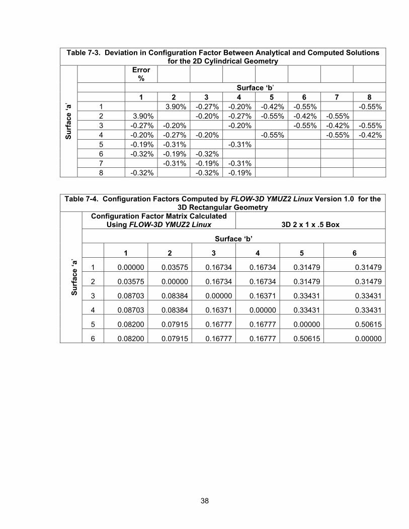
7.2 Thermal Radiation Configuration Factors Two geometrical configurations are chosen to test the capability of FLOW-3D YMUZ2 in computing the configuration factors. The first geometry consists of a planer configuration of two concentric cylinders. The outer cylinder has an inner diameter of 1.0 m [3.3 ft], and the inner cylinder has an outer diameter of 0.3 m [0.98 ft]. The Hottel method (Siegel and Howell, 1992) will be used to compute the configuration factors between each pair of surfaces for this case. The second geometry consists of a three- dimensional rectangular enclosure with dimensions of 2 m H 1 m H 0.5 m. The physics of the flow and related test matrix is described in Green (2006). 7.2.1 Test Input The test input used for the regression test is identical to that used in the validation study of FLOW-3D YMUZ2. FLOW-3D input files were developed to model the idealized cases (Green 2006). The computational domain for the cylindrical geometry is shown in Table 7-2 and for the rectangular geometry is shown in Figure 7-2. No flow solutions are performed, because the objective of this study is to evaluate the configuration factors. The input, output, and the postprocessed data are provided in the attached media in the directory \moist and rad\CF-calc. 7.2.2 Expected Test Results The acceptance criterion for this test case is that the configuration factors predicted by FLOW-3D shall be within 5 percent of the analytical predictions as described in the validation test plan (Green 2006). For the rectangular geometry, the analytical solution for the configuration factors is obtained using the Hottel cross section method. The configuration factors obtained analytically by Hottel’s cross string method are provided in the validation report (Green, 2006). For the rectangular enclosure, standard equations are available for each surface for configuration factors (Howell, 1982). 7.2.3 Test Results The configuration factors obtained from the analytical solution, FLOW-3D YMUZ2 Linux, and the deviation between them are listed in Tables 7-1, 7-2, and 7-3 respectively. The maximum deviation is 3.9 percent, which is within the acceptable limit as described in the validation test plan and report. Similarly, the configuration factors obtained from the analytical solution, FLOW-3D YMUZ2 Linux, and the deviation between them for the rectangular enclosure are listed in Tables 7-4, 7-5, and 7-6 respectively. The maximum deviation is 4.3 percent, which is within the acceptable limit as described in the validation test plan and report.

37
Table 7-1. Configuration Factors Computed by FLOW-3D YMUZ2 Linux Version 1.0 for the 2D Cylindrical Geometry
Configuration Factor
Matrix 2D Cylinders,
4 segments each
FLOW-3D,
71x71 Surface ‘b’ 1 2 3 4 5 6 7 8
1 0.0000 0.2342 0.1355 0.2342 0.2186 0.0402 0.0000 0.04022 0.2342 0.0000 0.2342 0.1355 0.0402 0.2186 0.0402 0.00003 0.1355 0.2342 0.0000 0.2342 0.0402 0.2186 0.04024 0.2342 0.1355 0.2342 0.0000 0.0402 0.0402 0.21865 0.7260 0.1334 0.0000 0.1334 0.0000 0.0000 0.0000 0.00006 0.1334 0.7260 0.1334 0.0000 0.0000 0.0000 0.0000 0.00007 0.0000 0.1334 0.7260 0.1334 0.0000 0.0000 0.0000 0.00008 0.1334 0.0000 0.1334 0.7260 0.0000 0.0000 0.0000 0.0000
Surf
ace
‘a’
Table 7-2. Configuration Factors Obtained From Analytical Solution for the 2D Cylindrical Geometry
Configuration Factor
Matrix 2D Cylinders,
4 segments each Exact Surface ‘b’ 1 2 3 4 5 6 7 8
1 0.2254 0.1358 0.2347 0.2196 0.0404 0.04042 0.2254 0.0000 0.2347 0.1358 0.0404 0.2195 0.0404 0.00003 0.1358 0.2347 0.0000 0.2347 0.0000 0.0404 0.2195 0.04044 0.2347 0.1358 0.2347 0.0000 0.0404 0.0000 0.0404 0.21955 0.7274 0.1339 0.0000 0.1339 0.0000 0.0000 0.0000 0.00006 0.1339 0.7274 0.1339 0.0000 0.0000 0.0000 0.0000 0.00007 0.0000 0.1339 0.7274 0.1339 0.0000 0.0000 0.0000 0.0000
Surf
ace
‘a’
8 0.1339 0.0000 0.1339 0.7274 0.0000 0.0000 0.0000 0.0000
38
Table 7-3. Deviation in Configuration Factor Between Analytical and Computed Solutions for the 2D Cylindrical Geometry
Error
% Surface ‘b’ 1 2 3 4 5 6 7 8
1 3.90% -0.27% -0.20% -0.42% -0.55% -0.55%2 3.90% -0.20% -0.27% -0.55% -0.42% -0.55% 3 -0.27% -0.20% -0.20% -0.55% -0.42% -0.55%4 -0.20% -0.27% -0.20% -0.55% -0.55% -0.42%5 -0.19% -0.31% -0.31% 6 -0.32% -0.19% -0.32% 7 -0.31% -0.19% -0.31%
Surf
ace
‘a’
8 -0.32% -0.32% -0.19%
Table 7-4. Configuration Factors Computed by FLOW-3D YMUZ2 Linux Version 1.0 for the 3D Rectangular Geometry
Configuration Factor Matrix Calculated Using FLOW-3D YMUZ2 Linux 3D 2 x 1 x .5 Box
Surface ‘b’
1 2 3 4 5 6
1 0.00000 0.03575 0.16734 0.16734 0.31479 0.31479
2 0.03575 0.00000 0.16734 0.16734 0.31479 0.31479
3 0.08703 0.08384 0.00000 0.16371 0.33431 0.33431
4 0.08703 0.08384 0.16371 0.00000 0.33431 0.33431
5 0.08200 0.07915 0.16777 0.16777 0.00000 0.50615
Surf
ace
‘a’
6 0.08200 0.07915 0.16777 0.16777 0.50615 0.00000

39
Table 7-5. Configuration Factors Obtained From Analytical Solution for the 3D Rectangular Geometry
Analytically Obtained Values of
Configuration Factor Matrix 3D 2 x 1 x .5 Box Surface ‘b’ 1 2 3 4 5 6
1 0.0362 0.1673 0.1673 0.3146 0.3146
2 0.0362 0.1673 0.1673 0.3146 0.3146
3 0.0837 0.0837 0.1653 0.3337 0.3337
4 0.0837 0.0837 0.1653 0.3337 0.3337
5 0.0787 0.0787 0.1669 0.1669 0.5090
Surf
ace
‘a’
6 0.0787 0.0787 0.1669 0.1669 0.5090
Table 7-6. Deviation in Configuration Factor Between Analytical and Computed Solutions for the 3D Rectangular Geometry
% Error Between the Computed Solution and Analytical Solution Surface ‘b’ 1 2 3 4 5 6
1 -1.18% 0.02% 0.02% 0.06% 0.06% 2 -1.18% 0.02% 0.02% 0.06% 0.06% 3 4.04% 0.22% -0.94% 0.18% 0.18% 4 4.04% 0.22% -0.94% 0.18% 0.18% 5 4.26% 0.64% 0.55% 0.55% -0.56%
Surf
ace
‘a’
6 4.26% 0.64% 0.55% 0.55% -0.56%

40
8 COMBINED HEAT TRANSFER TEST CASE
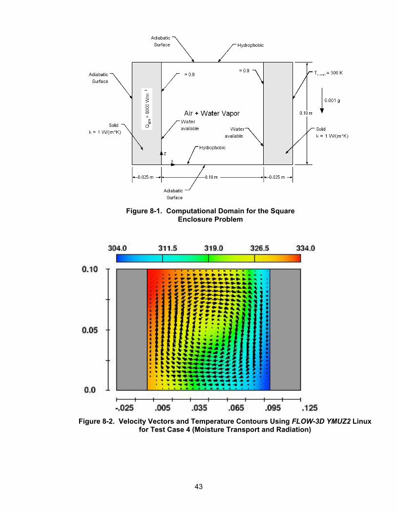
A number of simulations are performed in this section to test different modes of heat transfer and phase change by using the moisture transport and radiation modules. 8.1 Convection, Radiation, and Moisture Transport in an Enclosure A two-dimensional enclosure measuring 0.1 m H 0.1 m as shown in Figure 8.1 is used as the test bench for the present regression study. Both the left and right vertical walls are 0.025 m thick, and the right wall has an internal heat generation rate such that the heat flux at the inner surface is 200 W/m2. The outer surface of the left wall is adiabatic, but the right wall is treated as an isothermal obstruction with a temperature of 300 K. The emissivity of both the left and right walls is 0.9. The vertical walls are hydrophilic, which means that they are the source of water and under the existing temperature and concentration conditions in the flow. The upper and lower walls are adiabatic and do not participate in heat exchange. These walls are assumed to be transparent to radiation and therefore do not interact with the other walls via this mode. These walls are furthermore assumed to be hydrophobic; they do not participate in evaporation or condensation. The only interaction of these walls in the test case is to bound the flow and provide for viscous drag. The acceleration due to gravity is assumed to be only 0.001 g so that the flowfield for these geometric and thermal conditions will be laminar. Berkovsky and Polevikov (1977) provided the Nusselt number correlation for natural convection in a two-dimensional square enclosure that is used in the present study. The net mass transfer rate of water vapor through the enclosure will be estimated using the analogy of heat and mass transfer (Incropera and Dewitt, 1996). The radiation heat transfer will be analyzed using the methods of Siegel and Howell (1992) for gray diffuse surfaces in an enclosure. 8.1.1 Test Input The test input used for the regression test is identical to that used in the validation study of FLOW-3D YMUZ2. There are four different test cases that are simulated for the regression test. 1. Convection only 2. Convection with radiation 3. Convection with moisture transport 4. Convection, radiation, and moisture transport
In the original validation study, a number of grids were used to perform the mesh refinement study. In the present test, only the fine mesh simulations were performed. The input, output, and the postprocessed data are provided in the attached media in the directory \moist and rad\2-D-Box-Radiation-Moisture-conv.
41
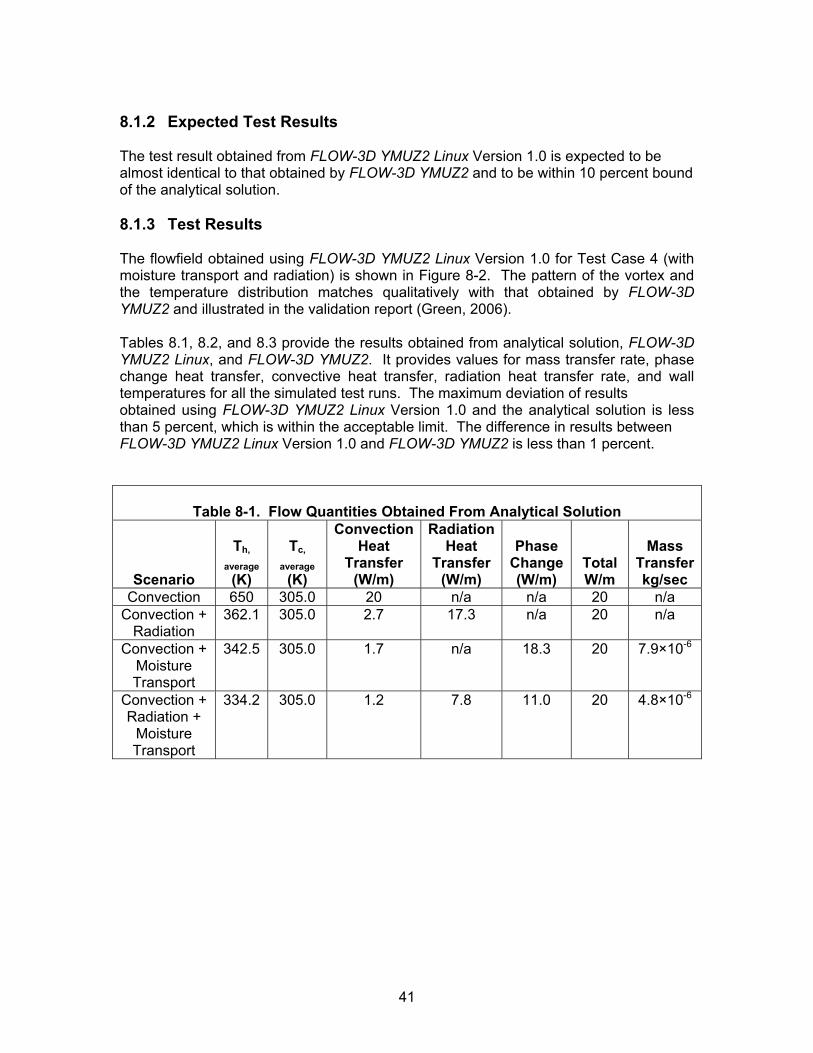
8.1.2 Expected Test Results The test result obtained from FLOW-3D YMUZ2 Linux Version 1.0 is expected to be almost identical to that obtained by FLOW-3D YMUZ2 and to be within 10 percent bound of the analytical solution. 8.1.3 Test Results The flowfield obtained using FLOW-3D YMUZ2 Linux Version 1.0 for Test Case 4 (with moisture transport and radiation) is shown in Figure 8-2. The pattern of the vortex and the temperature distribution matches qualitatively with that obtained by FLOW-3D YMUZ2 and illustrated in the validation report (Green, 2006). Tables 8.1, 8.2, and 8.3 provide the results obtained from analytical solution, FLOW-3D YMUZ2 Linux, and FLOW-3D YMUZ2. It provides values for mass transfer rate, phase change heat transfer, convective heat transfer, radiation heat transfer rate, and wall temperatures for all the simulated test runs. The maximum deviation of results obtained using FLOW-3D YMUZ2 Linux Version 1.0 and the analytical solution is less than 5 percent, which is within the acceptable limit. The difference in results between FLOW-3D YMUZ2 Linux Version 1.0 and FLOW-3D YMUZ2 is less than 1 percent.
Table 8-1. Flow Quantities Obtained From Analytical Solution
Scenario
Th,
average (K)
Tc,
average (K)
Convection Heat
Transfer (W/m)
Radiation Heat
Transfer (W/m)
Phase Change (W/m)
Total W/m
Mass Transfer kg/sec
Convection 650 305.0 20 n/a n/a 20 n/a Convection +
Radiation 362.1 305.0 2.7 17.3 n/a 20 n/a
Convection + Moisture Transport
342.5 305.0 1.7 n/a 18.3 20 7.9×10⁻⁶
Convection + Radiation +
Moisture Transport
334.2 305.0 1.2 7.8 11.0 20 4.8×10⁻⁶

42
Table 8-2. Flow Quantities Obtained From FLOW-3D YMUZ2
Scenario
Th,
average (K)
Tc,
average (K)
Convection Heat
Transfer (W/m)
Radiation Heat
Transfer (W/m)
Phase Change (W/m)
Total W/m
Mass Transfer kg/sec
Convection 646.2 304.5 20 n/a n/a 20 n/a Convection + Radiation
362.7 304.5 2.3 17.7 n/a 20 n/a
Convection + Moisture Transport
340.9 304.5 1.8 n/a 18.2 20 7.9×10⁻⁶
Convection + Radiation + Moisture Transport
333.8 304.5 1.3 7.9 11 20.2 4.8×10⁻⁶
Table 8-3. Flow Quantities Obtained From FLOW-3D YMUZ2 Linux
Scenario Th, average
(K) Tc, average
(K)
Convection Heat
Transfer (W/m)
Radiation Heat
Transfer (W/m)
Phase Change (W/m)
Total W/m
Mass Transfer kg/sec
Convection 643.18 (-.0%)
304.5 (0.1%)
20 n/a n/a 20.0 n/a
Convection + Radiation
362.67 (1.1%)
304.5 (-1.0)
2.3 (-2.0%)
17.7 (2.0%)
n/a 20.0 n/a
Convection + Moisture Transport
340.86 (-4.4%)
304.5((-1.4%)
2.2 n/a 17.8 20.0 7.8×10⁻⁶
Convection+ Radiation + Moisture Transport
333.8 (-1.5%)
304.5 (-1.7%)
1.6 (1%)
7.8 (0%)
11.0 (0%)
20.4 (2%)
4.8×10⁻⁶
43
Figure 8-2. Velocity Vectors and Temperature Contours Using FLOW-3D YMUZ2 Linux for Test Case 4 (Moisture Transport and Radiation)
Figure 8-1. Computational Domain for the Square Enclosure Problem
44
9 INDUSTRY EXPERIENCE FLOW-3D is used widely in industry for a number of applications like casting, aerospace, and free surface flows in civil engineering. However, no specific usage is cited in this report and the regression tests in this report are sufficient for validation of FLOW-3D YMUZ2 Linux Version 1.0.
10 CONCLUSION The regression test showed that FLOW-3D YMUZ2 Linux is successful in simulating the natural and forced convection flow and heat transfer along with radiation and moisture transport. Hence, the software can be considered validated by the method of regression analysis.
11 NOTES None.
12 REFERENCES Ampofo, F. and T.G. Karayiannis. “Experimental Benchmark Data for Turbulent Natural Convection in an Air-Filled Square Cavity.” International Journal of Heat and Mass Transfer. Vol. 46. pp. 3,551–3,572. 2003. Berkovsky, B.M. and V.K. Polevikov. “Numerical Study of Problems on High-Intensive Free Convection.” Heat Transfer and Turbulent Buoyant Convection. Vol. II. D.B. Spalding and H. Afgan, eds. Washington, DC: Hemisphere Publishing. pp. 443–455. 1977. Bird, R.B., W.E. Stewart, and E.N. Lightfoot. Transport Phenomena. New York City, New York: John Wiley & Sons. 1960. Churchill, S.W. and H.S. Chu. “Correlating Equations for Laminar and Turbulent-Free Convection from a Vertical Plate.” International Journal of Heat and Mass Transfer. Vol. 18. pp. 1,323–1,329. 1975. Das, K., S. Green, and C. Manepally. “FLOW-3D YMUZ2 Version 1. Users Manual.” San Antonio, Texas: CNWRA. 2007. Dubovsky, V., G. Ziskand, S. Druckman, E. Moshka, Y. Weiss, and R. Letan. “Natural Convection Inside Ventilated Enclosure Heated by Downward-Facing Plate: Experiments and Numerical Simulations.” International Journal of Heat and Mass Transfer. Vol. 44. pp. 3,155–3,168. 2001. Flow Science, Inc. <http://www.flow3d.com>. 2008.

45
______. “FLOW-3D® User’s Manual.” Version 9.2. Santa Fe, New Mexico: Flow Science, Inc. 2007a. ______. “FLOW-3D® Version 9.2 Release Notice.” Version 9.2. Santa Fe, New Mexico: Flow Science, Inc. 2007b. ______. “FLOW-3D® User’s Manual.” Version 9.0. Santa Fe, New Mexico: Flow Science, Inc. 2005. Fluent Inc. “FLUENT User’s Guide.” Version 4.52. Lebanon, New Hampshire: Fluent Inc. 1994. Green, S. “Software Requirements Description for the Modification of FLOW-3D To Include High-Humidity Moisture Transport Model and Thermal Radiation Effects Specific to Repository Drifts.” San Antonio, Texas: CNWRA. 2006. Green, S. and C. Manepally. “Software Validation Test Plan for FLOW-3D Version 9.” Rev. 1. San Antonio, Texas: CNWRA. 2006a. ______. “Software Validation Report for FLOW-3D YMUZ2.” Rev. 1. San Antonio, Texas: CNWRA. 2006b. Howell, J.R. A Catalog of Radiation Configuration Factors. New York City, New York: McGraw-Hill Book Company. 1982. Incropera, F.P. and D.P. Dewitt. Fundamentals of Heat and Mass Transfer 4th Edition. pp. 487–490. New York City, New York: John Wiley & Sons, Inc. 1996. Kuehn, T.H. and R.J. Goldstein. “An Experimental Study of Natural Convection Heat Transfer in Concentric and Eccentric Horizontal Cylindrical Annuli.” ASME Journal of Heat Transfer. Vol. 100. pp. 635–640. 1978. Siegel, R. and J.R. Howell. Thermal Radiation Heat Transfer. 3rd Edition. Washington, DC: Hemisphere Publishing Corporation. 1992.