Flood simulation and visualization Milan Kollinger1, Karel Vondráček2, Václava Šeblová3,

Jaroslav Zdražil4, Jakub Jirka5, Lucie Vokounová6 University of West Bohemia

Pilsen, Czech Republic

Abstract Natural phenomena simulation and visualization are becoming very useful in today's information community. A typical example is the last year's floods in the Czech Republic. Flood task forces which had the flood limits of different flood conditions were able to determine on persons and movable property evacuation. This article describes the utilization of geographic information systems (GIS) at flood simulation and visualization. Simple simulation flood model implementation into GIS, in particular ArcView 8.x release, is described. In this paper can be also found: the method of data preparing, the formulas used in calculations and flood simulation on the Mže and Radbuza Rivers results evaluation.

Keywords: flood, simulation, visualization, GIS, DTM.

1 Introduction A human property is to forget things which do not repeat themselves very often. A typical example is the last year’s floods in the Czech Republic and their catastrophic impacts which were from a great part caused by a human carelessness. During the 20th century no larger flood occurred in the Central Europe, and people very quickly forgot about the danger of floods in the areas around water courses. A goal of this project was to create a tool which shows the peril of floods and helps people in making their decisions [3]. We have chosen segments of the Mže River and the Radbuza River including their immediate surroundings as areas of interest. These rivers flow through the city of Pilsen and have great influence on its structure.

Unfortunately, the project has been solved after the last year’s floods, which proved the fact that many local authorities and even municipalities situated in flood districts do not have any flooding limits at their disposal.

Flood limits serve the flood task force to analyze flooded areas that should be evacuated. Flood limits also serve the municipal and building offices to survey danger areas for building new houses, industrial estates etc. So it is evident that in order to minimize the flood damages the knowledge of flood limits is necessary.

The aim of this project was the implementation of a simple simulation model for flood model calculation into a geographic information system (GIS). The term ‘flood model’ means a digital model in raster form where cell values correspond to river levels during the flood. Afterwards there is a possibility to visualize and analyze these models in GIS. At the beginning of the project we analyzed existing software solving this given problem. During the analysis we discovered existence of a commercial software MIKE for the flood limits computations. Further on, Department of Hydraulics and Hydrology on the Czech Technical University in Prague also works on flood limit computations. Due to the fact that our specialization is Geodesy and GIS, the goal was not creation of an accurate simulation tool but implementation of a simple simulation model, as already mentioned above, into existing GIS software – specifically into ESRI ArcView in 8.x release. As for flood limits computation, applying GIS is quite convenient because most of the required entry data is obtained from geodetic or aerial photographic surveying and easy to work with in GIS. Using the resultant flood model we are able to, e.g., locate flood limits, survey flooded objects or create bathimetric map. Therefore, the flood is calculated in ArcView environment, in which loading Digital Terrain Model (DTM), cross-profiles database and joining dynamic library before flood model computation itself is necessary. DTM is a mathematical formulation of altitudinal proportions in given geo-graphic area (see Figure 1).

The method of simple simulation model implementation into ArcView is described in the following. Next, you can read about the input data for calculations preparing, the used formulas and algorithms. Finally, you can find the records evaluation at calculations on the Mže and Radbuza Rivers in Pilsen.

1 milan.kollinger@seznam.cz 2 vondr551@centrum.cz 3 vsebl@email.cz 4 zeryk@students.zcu.cz 5 jirkaja@centrum.cz 6 vokynko@seznam.cz

Figure 1: Digital Terrain Model of the Mže River surrounding with cross-profiles.

2 Problem solving, input data As mentioned above, we solved the flood model computation in ArcView. This software is a scalable system for geographic data creation and management. Extension with the assistance of built-in Visual Basic for Applications development environment or Component Object Model (COM) modular technology is supported, therefore its functionality can be extended. In this instance we utilized the possibility of programming a stand-alone module in MS Visual Basic 6 development environment, dynamic library is concerned [2].

It was necessary to devise a flood model calculation algorithm before programming itself. Our aim, as mentioned above, was to create and apply a simple simulation model for flood computation. It is why we implemented simple hydrological formulas from textbook [1]. These formulas are implemented in a program module of the dynamic library and they are replaceable with others using more accurate method of flood model calculation in the future. Reason for this implementation, as already mentioned, was the fact that our specialization is Geodesy and GIS. Creating of more accurate formulas or simulation model is the hydrologist affair. On the other hand, work of the geodesists and experts on GIS, among whom we can rank, is primarily preparation of data for calculations and implementation of simulation models into GIS, through which most of geodata is processed these days. ‘Geodata’ means data

which contains some spatial piece of information, such as a map, DTM, an aerial photograph, etc.

General information about GIS domain can be found in [4] or [5].

2.1 Input data Data preparation is necessary to make before the very beginning of flood model calculation. In the case of flood simulation it concerns geodata preparing, primarily the DTM, which was provided for our student use by the firm in ESRI GRID format. This format saves all terrain points in a raster form, in which the cell value accords with elevation of a given point. In this instance, one cell of raster corresponds to area of 2 x 2 meters. All the geodata we use is located in the coordinate system of the Uniform Trigonometric Cadastral Network (S-JTSK) and the elevation coordinate of each individual point was determined in the elevation system “Balt – after Adjustment” (Bpv). These coordinate systems are binding geodetic reference systems in the Czech Republic and thus also used for the resulting flood model. It is very advantageous, because it allows us to enter other layers of geodata (e.g., Digital Cadastral Map, planimetry of the Fundamental Base of Geographic Data – ZABAGED – and other map series) into GIS (ArcView). Subsequently we can make another analysis of floods with all layers of geodata in GIS.

Further, it was necessary to prepare cross-profiles of

water flow for calculations. For making cross-profiles suggestion and results visualization we used orthophotomaps. The orthophotomap is a transformed aerial photography. It is created by tracing of aerial photography corresponding to central projection so that the resulting picture (orthophotomap) would be in parallel projection demanded from cartographical projections. We applied cross-profiles generated from DTM because we did not have their real surveying at our disposal. Cross-profiles were designed in 2D form, approximately perpendicular to water course. Afterwards we projected the 2D lines on DTM and so they were converted into three-dimensional space and gained the third Z-coordinate. In this instance, Z-coordinate matched elevation in the Bpv elevation system.

Finally, it was needful to create a database of individual cross-profiles characteristics. There exist several characteristics and moreover they can change in the course of the profile. We split each cross-profile into three parts: the river bed, left bank and right bank. Different characteristics may be then set in each part of the cross-profile. It concerns coefficient of surface roughness (roughness coefficient) and river bed gradient. To determine roughness coefficient, we used the textbook [1]. However, the adjustment of gradient rate parameters was very problematic because we did not dispose accurately measured gradients in individual cross-profiles. River gradients may be counted from the elevations but measuring out the elevations from our DTM was not quite correct because it does not have high fidelity and even little changes in gradients proved too much influence. Therefore we chose the following method of gradient rate setting.

After the last year’s floods we gained boundary lines of flooded areas plotted from an aerial photograph taken in 14th August 2002 (one day after critical flood flow in Pilsen) corresponding to the flow rate Q. We always determined two points of intersection with the lines for each single cross-profile and then rolled out to them the elevation from DTM. Average of observed elevation values matched the water level in the given cross-profile at the flow rate Q. Thereafter we set the gradient rates so that calculated flood level elevation for given cross-profile would fit the mentioned average elevation on condition of entering the flow rate Q in calculations beforehand. Thereby we achieved the calibration at the same time.

The last parameter is the percentage increment of the flow rate related to the entered flow rate. The tributaries may be taken into consideration this way. All these characteristics were saved in MS Access database and successively read during the calculations.

2.2 Calculation process, algorithm The whole calculation can be divided into two parts – into level of water calculation for individual cross-profiles and into interpolation between cross-profiles.

Algorithm for level of water calculation in the given profile is relatively complicated. Input is the flow rate but it is not possible to find out level only by putting into formula. On the other side, it is possible to count the flow rate Q with putting the level of water h and several other known values. That is why we change the level of water value h and count the flow rate Q in consecutive iteration in the algorithm. Iteration stops when value Q approximately matches the desired flow rate in the cross-profile. Then the actual level h represents flood level in the given profile.

For flow rate calculation we used the following formulas from hydromechanics [1] depending on the area, wetted perimeter, roughness of river bed and gradient of river bed:

vSQ ⋅= Ricv ⋅=

611 R

nc ⋅=

OSR =

after conversion: 121

32

35

−−

⋅⋅⋅= niOSQ where:

Q – flow rate S – flow area O – wetted perimeter v – flow velocity c – velocity coefficient R – hydraulic radius i – gradient n – roughness coefficient (range from 0.016 to 0.16) The wetted perimeter O, the flow area S and (from

that) the flow rate QPOC is counted at each change of the water level. The values of roughness and gradient are known constants. If the water level exceeds any bank of the river bed, the flow calculation is divided into three parts (see Figure 2), for: the river bed, right bank and left bank. Each part has not only different values of area and perimeter but also roughness and gradient. Therefore we count the flow rate for each part separately and get the resultant flow for the given cross-profile by counting up the flow rates from separate parts. Algorithm counts the flow rates for water levels corresponding to heights of the left and right bank and maximum flow rate which we are able to count. The entered flow rate is tested for being less than maximum one before calculation. If it is valid, the calculation continues.

Figure 2: The method of cross-profile dividing into three parts according to the left and right bank line.

Figure 3: The flow rates according to the left or right bank line.

Condition Schematic drawing Description of situation Initial level of water

Q<QL and Q<Q

P

Level of water is not higher than river bank lines. Calculation proceeds only in the river bed.

lowest point in the river bed

QP<Q<Q

L

The water level overflows the right bank line. Calculation proceeds in the river bed and on the right bank.

height of the right bank line

QL<Q<Q

P

The water level overflows the left bank line. Calculation proceeds in the river bed and on the left bank.

height of the left bank line

Q>QL and Q>Q

P

The water level overflows the right and also the left bank line. Calculation proceeds in the river bed and on both banks.

height of higher of bank lines, max(Q

L, Q

P)

Table 1: There can arise four cases of water spilling during the flood.

Comparing the entered flow rate with flows QL and

QP (the flows when the water level corresponds to the left or to the right river bank line – Figure 3) we find out whether the spill-over from the river bed happens and we get the initial level of water. There can arise four cases, see Table 1.

The water level rises in specific steps in iteration (initial step is set on 0.5 m). If we exceed a desired flow rate for the given level of water, we return one step back and reduce the step. Step after the first reduction has the value 0.05 m and during the next reduction is divided into halves. In the main it corresponds with interval bisection. The mentioned iteration is ended in the moment when the calculated flow rate roughly equals the demanded flow in the cross-profile.

The algorithm of water level interpolation between

individual cross-profiles firstly creates a new GRID. This GRID represents the flood model and has the same cell size and spatial location as DTM. Further we interpolate the value for each cell of a new GRID. Interpolation is linear and by perpendiculars: At first we find the cross-profiles between which the interpolated point is placed. We create the perpendiculars from point to both cross-profiles and count the distance between the point and each of the profiles (d1, d2). Ratio of distances is used as an interpolation ratio. With this value we multiply the difference of flood level in neighbouring profiles. Afterwards we add this result to that one of the neighbouring cross-profiles which has lower elevation above sea level. This final value represents the flood elevation in the given place which will be put into the GRID cell.

Flow area: S

1 - the river bed

S2

- the left bank S

3 - the right bank

Wetted perimeter: O

1 - the river bed

O2

- the left bank O

3 - the right bank

Height of: H

L - the left bank line

HR - the right bank line

Maximal flow rate: Q

L - according to H

L Q

R - according to H

R

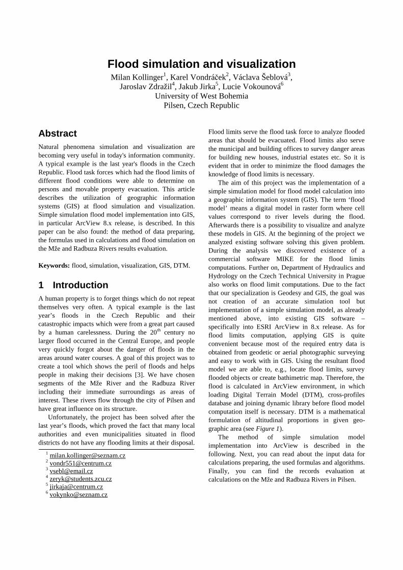
The interpolation formula:

( )1221

11 hh

dddhh −⋅+

+=

To get a real flood model, we further have to crop the

resulting GRID with DTM. It will be accomplished making a simple requirement in which the elevations of the same cells of GRID and DTM will compare. If the elevation of DTM cell is higher than GRID one then the elevation in GRID cell changes to NoDataValue (non-valued cell). If the elevation of DTM is less than elevation of GRID then nothing changes.

3 Calculation results and evaluation

Accuracy of calculated flood limits is primarily influenced by DTM. In this instance, the accuracy of

input data for DTM was ±35 cm. In GIS, however, it is possible to supplement input data with more exact data, such as 3D coordinates from geodetic surveyings. Thereafter we might create new DTM of higher-quality and give precision to subsequently calculated flood model in this way.

Furthermore, the accuracy depends on the access selected for flood model computation. In this instance we applied rather elementary formulas, which do not take into consideration all the effects, such as geological subsoil, water dynamics, sediment shifting, etc. It certainly has a substantial influence on calculation results. The fact of the matter is that calculation in the initiated method, with the assistance of the library programmed by us, can be used without any problems for the segments of water flows which do not take in any significant tributaries. If we intend to apply this computation even for water flow with strong tributary, it is necessary to modify parameters of calculation according to it.

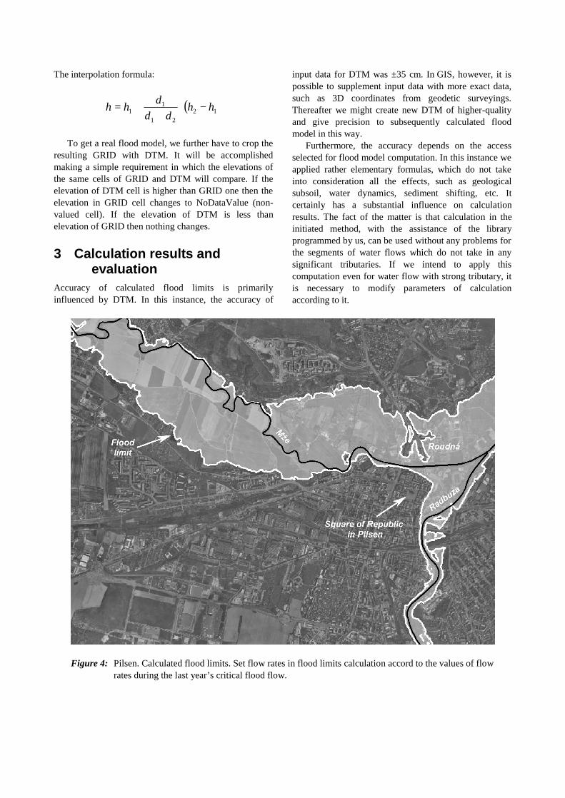
Figure 4: Pilsen. Calculated flood limits. Set flow rates in flood limits calculation accord to the values of flow rates during the last year’s critical flood flow.

Figure 5: The centre of Pilsen. Calculated flood limits. Set flow rates in flood limits calculation accord to the values of flow rates during the last year’s critical flood flow.

This situation emerged also in the case of tributary

of the Úhlava into the Radbuza and in the confluence of the Mže and the Radbuza Rivers (see Figure 4 and 5). We solved this problem increasing flow rate at several cross-profiles in front of the confluence itself. Thereby we also achieved the increase of calculated flood level at these cross-profiles. The resulting flood model proves that the amount of water flowing into a stream affects the flood not only behind the confluence of rivers but also in front of it. This phenomenon set in during the last year's flood in Pilsen – the city situated on the Mže, which was strongly affected by floodwater from the Radbuza. Many experts agreed on the fact that the suburb of Pilsen – Roudná, located on the bank of the Mže, cca 300 m in front of the Radbuza tributary, was in the event flooded by the water from the Radbuza.

Last but not least, the resulting flood model is very much determined by the parameters of constituent cross-profiles. Among such parameters the roughness coefficient and gradient of river bed belong. The roughness coefficient can continuously change in the whole length of the cross-profile. This given fact we did not take into account in this instance and in cross-

profile there is an option to set roughness coefficient of the left bank, river bed and right bank. In accordance with this fact, individual cross-profiles were designed in order not to make the roughness coefficient vary in the course of cross-profile too much. Gradients can be also modified for the right bank, river bed and left bank.

Therefore the evaluation of calculated resulting limits is very problematic. However, we disposed of a map copy containing flood limits of the really flooded areas in Pilsen from the last year's floodings. Using these limits we were able to verify the accuracy of our calculations and then to set flow rates in river valleys corresponding to the last year's floods and accomplish computation of flood model. Subsequently we evaluated flood limits. In computations we considered the fact that during the last year's floods flow rate on the Mže was approximately corresponding with ten-year flood and flow rate of fifty-year flood on the Radbuza. Thereafter the flood on the Radbuza was highly affecting flood level on the Mže in confluence of these rivers. Going through visual control comparison of calculated limits with the limits corresponding to the real flood, we could observe that

both limits matched sufficiently in 80%. According to these results we can certify that calculated floods will be credible for flow rates in the range of 90 – 300 m3/s. Counting the flood level complying with lower flow rates, DTM indicates too much inexactness and therefore the resulting flood model would be very affected by these inaccuracies. On the other hand in the flow rates above 300 m3/s, there is no way to verify the accuracy of calculated model, respectively evaluated flood limits. The primary reason is that we did not dispose any check points, which would correspond to the initiated flood at flow rate of 300 m3/s.

4 Conclusion The project itself can be divided into several stages. In the first stage, as introduced, we confirmed our capability of applying GIS for flood simulations. We succeed and the results of this task were quite satisfying. Now we are at the beginning of the second stage, attempting to particularize the simulation model so that it would comprise more influences during floods and give to the resulting flood models more precision. For this purpose we are in the need of close cooperation with hydrologists, who deal with projection of simulation flood models. As for the computation, we contemplate to apply data from state map works which would noticeably reduce expenses on obtaining input data. As the most expensive data includes DTM, we intend to utilize contour lines from the state map series ZABAGED for its creation and subsequently give DTM precision by applying another geodetic surveying available. If we manage to elaborate the calculations and prove the possible application of ZABAGED for preparation of input data (primarily for creation of DTM), small and midsized municipalities would be able to acquire accomplished calculation of not so exact, but also less expensive flood model of their regions. Thereafter it can serve for territorial planning of municipalities or for critical and rescue staff in a case of floods.

Acknowledgements This work is supervised by Václav Skala and was supported by the project MŠMT 235200005. The authors would like to thank to Karel Jedlička for professional consultations at work with GIS. Next, to Petr Plný for professional consultations from hydrology and Ivana Kolingerová for editing this report. Our thanks also belong to data providers – the Czech Office for Surveying, Mapping and Cadastre (Prague) and firm Georeal s.r.o. (Pilsen).

References [1] V.Havlík, I.Marešová: HYDRAULIKA I.,

Textbook (in Czech), ČVUT, Prague, 1994

[2] ESRI ArcObjects [online] . c2003, last revision 3.10.2002 [cit.6-1-2003]. http://arconline.esri.com/arcobjectsonline/

[3] R.W.Greene: Confronting Catastrophe: A GIS Handbook, ESRI, Redlands – California, 2002

[4] P.A.Burrough, R.A.McDonnell: Principles of Geographical Information Systems, Oxford University Press, New York, 1998

[5] J.Tuček: Geographic Information Systems – Principles and Practice, Computer Press, Prague, 1998