flight tests of a remaining flying time prediction system

1

Flight Tests of a Remaining Flying Time Prediction System for Small

Electric Aircraft in the Presence of Faults

Edward F. Hogge1, Chetan S. Kulkarni2, Sixto L. Vazquez3, Kyle M. Smalling4, Thomas H. Strom5, Boyd L. Hill6, and

Cuong C. Quach7

1,4,5Northrop Grumman Technology Services, NASA Langley Research Center, Hampton, Virginia 23681 [email protected]

[email protected]

[email protected]

2Stinger Ghaffarian Technologies, Inc., NASA Ames Research Center, Moffett Field, California 94035 [email protected]

3,7NASA Langley Research Center, Hampton, Virginia 23681

[email protected]

[email protected]

6Analytical Mechanics Associates, Inc., NASA Langley Research Center, Hampton, Virginia 23681 [email protected]

ABSTRACT

This paper addresses the problem of building trust in the

online prediction of a battery powered aircraft’s remaining

flying time. A series of flight tests is described that make use

of a small electric powered unmanned aerial vehicle (eUAV)

to verify the performance of the remaining flying time

prediction algorithm. The estimate of remaining flying time

is used to activate an alarm when the predicted remaining

time is two minutes. This notifies the pilot to transition to the

landing phase of the flight. A second alarm is activated when

the battery charge falls below a specified limit threshold. This

threshold is the point at which the battery energy reserve

would no longer safely support two repeated aborted landing

attempts. During the test series, the motor system is operated

with the same predefined timed airspeed profile for each test.

To test the robustness of the prediction, half of the tests were

performed with, and half were performed without, a

simulated powertrain fault. The pilot remotely engages a

resistor bank at a specified time during the test flight to

simulate a partial powertrain fault. The flying time prediction

system is agnostic of the pilot’s activation of the fault and

must adapt to the vehicle’s state. The time at which the limit

threshold on battery charge is reached is then used to measure

the accuracy of the remaining flying time predictions.

Accuracy requirements for the alarms are considered and the

results discussed.

1. INTRODUCTION

Improvements in battery storage capacity have made it

possible for general aviation vehicle manufacturers to

consider electrically-powered solutions. The development of

trust in battery remaining operating time estimates, however,

is currently a significant obstacle when considering adoption

of electrical propulsion systems in aircraft (Patterson,

German & Moore, 2012). There are several ways in which

predicting remaining operating time is more complicated for

battery-powered vehicles than it is for vehicles with a

conventionally-powered liquid-fueled combustion system.

Unlike a liquid-fueled system, where the fuel tank’s volume

remains unchanged over successive refueling procedures, a

battery’s charge storage capacity will diminish over time.

Another complicating feature of a battery system is the time-

varying relationship between battery output power and

battery current draw. Whereas a conventional liquid

combustion system uses an approximately constant amount

of liquid fuel to produce a given motive power, the power

from a battery system is equal to the product of battery

voltage and current. Thus, as batteries are discharged, their

voltages drop, and they will lose charge at a faster rate.

Previous papers introduced several new tools for battery

discharge prediction onboard a small electric aircraft. A

series of ground tests similar to the flight tests used in this

Edward Hogge et al. This is an open-access article distributed under the terms of the Creative Commons Attribution 3.0 United States License,

which permits unrestricted use, distribution, and reproduction in any

medium, provided the original author and source are credited.

mailto:[email protected]




ANNUAL CONFERENCE OF THE PROGNOSTICS AND HEALTH MANAGEMENT SOCIETY 2017

2

work are described in Hogge, Bole, Vazquez, Celaya, Strom,

Hill, Smalling & Quach (2015), and a battery equivalent

circuit model used to simulate the battery state is described in

Bole, Teubert, Quach, Hogge, Vazquez and Goebel (2013).

The model’s battery capacity, internal resistance and other

parameters were identified through two laboratory

experiments that used a programmed load. In one experiment

the batteries were slowly discharged. In the other experiment

a repeated pulsed loading discharge was done. Current and

voltage profiles logged during flights of a small electric

airplane further tuned the battery model (Quach, Bole,

Hogge, Vazquez, Daigle, Celaya, Weber & Goebel, 2013).

The use of a flight plan with upper and lower uncertainty

bounds on the required energy to complete the mission

successfully was presented along with an approach to identify

additional parasitic battery loads (Bole, Daigle & Gorospe,

2014). This paper describes results of initial flight tests to

assess the performance of an alarm that warns system

operators when the estimated remaining flying time falls

below a certain threshold.

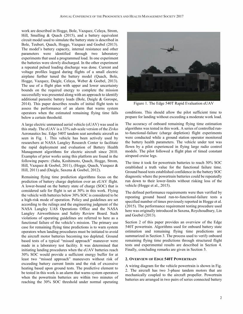
A large electric unmanned aerial vehicle (eUAV) was used in

this study. The eUAV is a 33% sub-scale version of the Zivko

Aeronautics Inc. Edge 540T tandem seat aerobatic aircraft as

seen in Fig. 1. This vehicle has been actively used by

researchers at NASA Langley Research Center to facilitate

the rapid deployment and evaluation of Battery Health

Management algorithms for electric aircraft since 2010.

Examples of prior works using this platform are found in the

following papers: (Saha, Koshimoto, Quach, Hogge, Strom,

Hill, Vazquez & Goebel, 2011), (Hogge, Quach, Vazquez &

Hill, 2011) and (Daigle, Saxena & Goebel, 2012).

Remaining flying time prediction algorithms focus on the

prediction of battery charge depletion over an eUAV flight.

A lower-bound on the battery state of charge (SOC) that is

considered safe for flight is set at 30% in this work. Flying

the vehicle with batteries below 30% SOC is considered to be

a high-risk mode of operation. Policy and guidelines are set

according to the rulings and the engineering judgment of the

NASA Langley UAS Operations Office and the NASA

Langley Airworthiness and Safety Review Board. Such

violations of operating guidelines are referred to here as a

functional failure of the vehicle’s mission. The primary use

case for remaining flying time predictions is to warn system

operators when landing procedures must be initiated to avoid

the aircraft motor batteries becoming too depleted. Ground

based tests of a typical “missed approach” maneuver were

made in a laboratory test facility. It was determined that

initiating landing procedures when the eUAV batteries reach

30% SOC would provide a sufficient energy buffer for at

least two “missed approach” maneuvers without risk of

exceeding battery current limits and the risk of excessive

heating based upon ground tests. The predictive element to

be tested in this work is an alarm that warns system operators

when the powertrain batteries are within two minutes of

reaching the 30% SOC threshold under normal operating

conditions. This should allow the pilot sufficient time to

prepare for landing without exceeding a moderate work load.

The accuracy of onboard remaining flying time estimation

algorithms was tested in this work. A series of controlled run-

to-functional-failure (charge depletion) flight experiments

were conducted while a ground station operator monitored

the battery health parameters. The vehicle under test was

flown by a pilot experienced in flying large radio control

models. The pilot followed a flight plan of timed constant

airspeed cruise legs.

The time it took for powertrain batteries to reach 30% SOC

established a truth value for the functional failure time.

Ground based tests established confidence in the battery SOC

diagnostic where the powertrain batteries could be repeatedly

run down to their lower-limits without risking loss of the

vehicle (Hogge et al., 2015).

The defined performance requirements were then verified by

repeating ground based run-to-functional-failure tests a

specified number of times previously reported in Hogge et al.

(2015). The performance requirement testing procedure used

here was originally introduced in Saxena, Roychoudhury, Lin

and Goebel (2013).

Section 2 of this paper provides an overview of the Edge

540T powertrain. Algorithms used for onboard battery state

estimation and remaining flying time predictions are

summarized in Section 3. The process used to verify onboard

remaining flying time predictions through structured flight

tests and experimental results are described in Section 4.

Finally, concluding remarks are given in Section 5.

2. OVERVIEW OF EDGE 540T POWERTRAIN

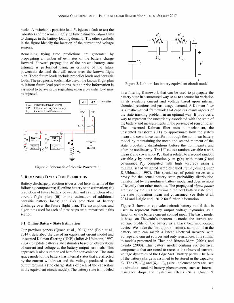
A wiring diagram for the vehicle powertrain is shown in Fig.

2. The aircraft has two 3-phase tandem motors that are

mechanically coupled to the aircraft propeller. Powertrain

batteries are arranged in two pairs of series connected battery

Figure 1. The Edge 540T Rapid Evaluation eUAV


3

packs. A switchable parasitic load Rp injects a fault to test the

robustness of the remaining flying time estimation algorithms

to changes in the battery loading demand. The other symbols

in the figure identify the location of the current and voltage

sensors.

Remaining flying time predictions are generated by

propagating a number of estimates of the battery charge

forward. Forward propagation of the present battery state

estimate is performed using an estimate of the future

powertrain demand that will occur over the known flight

plan. These future loads include propeller loads and parasitic

loads. The prognostic tools make use of the known flight plan

to inform future load predictions, but no prior information is

assumed to be available regarding when a parasitic load may

be injected.

3. REMAINING FLYING TIME PREDICTION

Battery discharge prediction is described here in terms of the

following components; (i) online battery state estimation; (ii)

prediction of future battery power demand as a function of an

aircraft flight plan; (iii) online estimation of additional

parasitic battery loads; and (iv) prediction of battery

discharge over the future flight plan. The assumptions and

algorithms used for each of these steps are summarized in this

section.

3.1. Online Battery State Estimation

Our previous papers (Quach et al., 2013) and (Bole et al.,

2014), described the use of an equivalent circuit model and

unscented Kalman filtering (UKF) (Julier & Uhlmann, 1997,

2004) to update battery state estimates based on observations

of current and voltage at the battery output terminals. This

approach is also summarized here for convenience. The state

space model of the battery has internal states that are affected

by the current withdrawn and the voltage produced at the

output terminals (the charge states of each of the capacitors

in the equivalent circuit model). The battery state is modeled

in a filtering framework that can be used to propagate the

battery state in a structured way so as to account for variation

in its available current and voltage based upon internal

chemical reactions and past usage demand. A Kalman filter

is a mathematical framework that captures many aspects of

the state tracking problem in an optimal way. It provides a

way to represent the uncertianty associated with the state of

the battery and measurements in the presence of sensor noise.

The unscented Kalman filter uses a mechanism, the

unscented transform (UT) to approximate how the state’s

mean and covariance transform through the nonlinear battery

model by maintaining the mean and second moment of the

state probability distributions before the nonlinearity and

after the nonlinearity. The UT takes a random variable 𝐱 with

mean and covariance 𝐏𝑥𝑥 that is related to a second random

variable 𝐲 by some function 𝐲 = 𝐠(𝐱) with mean and

covariance 𝐏𝑦𝑦 computed with high accuracy using a

minimal set of weighted samples called sigma points (Julier

& Uhlmann, 1997). This special set of points serves as a

proxy for the actual battery state probability distribution

transformed by the nonlinear battery model and does so more

efficiently than other methods. The propagated sigma points

are used by the UKF to estimate the next battery state from

the state population mean and covariance. See Bole et al,

2014 and Daigle et al, 2012 for further information.

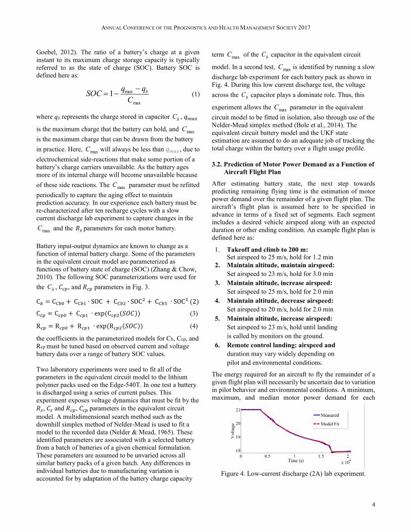
Figure 3 shows an equivalent circuit battery model that is

used to represent battery output voltage dynamics as a

function of the battery current control input. The basic model

is based on Thevenin’s theorem to model the current and

voltage profile of the battery as a black box input-output

device. We make the first-approximation assumption that the

battery state can match a linear electrical network with

voltage and current sources and only resistances. It is similar

to models presented in Chen and Rincon-Mora (2006), and

Ceralo (2000). This battery model contains six electrical

components that are tuned to recreate the observed current-

voltage dynamics of the Edge 540T battery packs. The bulk

of the battery charge is assumed to be stored in the capacitor

𝐶𝑏. The (𝑅𝑠, 𝐶𝑠) and (𝑅𝑐𝑝, 𝐶𝑐𝑝) circuit element pairs are used

to simulate standard battery phenomenon, such as internal

resistance drops and hysteresis effects (Saha, Quach &

Figure 3. Lithium-Ion battery equivalent circuit model

Figure 2. Schematic of electric Powertrain.


4

Goebel, 2012). The ratio of a battery’s charge at a given

instant to its maximum charge storage capacity is typically

referred to as the state of charge (SOC). Battery SOC is

defined here as:

max

max1C

qqSOC b

(1)

where qb represents the charge stored in capacitor bC , 𝑞𝑚𝑎𝑥

is the maximum charge that the battery can hold, and maxC

is the maximum charge that can be drawn from the battery

in practice. Here, maxC will always be less than 𝑞𝑚𝑎𝑥 , due to

electrochemical side-reactions that make some portion of a

battery’s charge carriers unavailable. As the battery ages

more of its internal charge will become unavailable because

of these side reactions. The maxC parameter must be refitted

periodically to capture the aging effect to maintain

prediction accuracy. In our experience each battery must be

re-characterized after ten recharge cycles with a slow

current discharge lab experiment to capture changes in the

maxC and the 𝑅𝑠 parameters for each motor battery.

Battery input-output dynamics are known to change as a

function of internal battery charge. Some of the parameters

in the equivalent circuit model are parameterized as

functions of battery state of charge (SOC) (Zhang & Chow,

2010). The following SOC parameterizations were used for

the bC , 𝐶𝑐𝑝, and 𝑅𝑐𝑝 parameters in Fig. 3.

C𝑏 = C𝐶𝑏0 + C𝐶𝑏1 ∙ SOC + C𝐶𝑏2 ∙ SOC2 + C𝐶𝑏3 ∙ SOC3 (2)

C𝑐𝑝 = C𝑐𝑝0 + C𝑐𝑝1 ∙ exp (C𝑐𝑝2(𝑆𝑂𝐶)) (3)

R𝑐𝑝 = R𝑐𝑝0 + R𝑐𝑝1 ∙ exp (R𝑐𝑝2(𝑆𝑂𝐶)) (4)

the coefficients in the parameterized models for Cb, Ccp, and

Rcp must be tuned based on observed current and voltage

battery data over a range of battery SOC values.

Two laboratory experiments were used to fit all of the

parameters in the equivalent circuit model to the lithium

polymer packs used on the Edge-540T. In one test a battery

is discharged using a series of current pulses. This

experiment exposes voltage dynamics that must be fit by the

𝑅𝑠, 𝐶𝑠 and 𝑅𝑐𝑝, 𝐶𝑐𝑝 parameters in the equivalent circuit

model. A multidimensional search method such as the

downhill simplex method of Nelder-Mead is used to fit a

model to the recorded data (Nelder & Mead, 1965). These

identified parameters are associated with a selected battery

from a batch of batteries of a given chemical formulation.

These parameters are assumed to be unvaried across all

similar battery packs of a given batch. Any differences in

individual batteries due to manufacturing variation is

accounted for by adaptation of the battery charge capacity

term maxC of the bC capacitor in the equivalent circuit

model. In a second test, maxC is identified by running a slow

discharge lab experiment for each battery pack as shown in

Fig. 4. During this low current discharge test, the voltage

across the bC capacitor plays a dominate role. Thus, this

experiment allows the maxC parameter in the equivalent

circuit model to be fitted in isolation, also through use of the

Nelder-Mead simplex method (Bole et al., 2014). The

equivalent circuit battery model and the UKF state

estimation are assumed to do an adequate job of tracking the

total charge within the battery over a flight usage profile.

3.2. Prediction of Motor Power Demand as a Function of

Aircraft Flight Plan

After estimating battery state, the next step towards

predicting remaining flying time is the estimation of motor

power demand over the remainder of a given flight plan. The

aircraft’s flight plan is assumed here to be specified in

advance in terms of a fixed set of segments. Each segment

includes a desired vehicle airspeed along with an expected

duration or other ending condition. An example flight plan is

defined here as:

1. Takeoff and climb to 200 m: Set airspeed to 25 m/s, hold for 1.2 min

2. Maintain altitude, maintain airspeed:

Set airspeed to 23 m/s, hold for 3.0 min

3. Maintain altitude, increase airspeed:


4. Maintain altitude, decrease airspeed:


5. Maintain altitude, increase airspeed:

Set airspeed to 23 m/s, hold until landing

is called by monitors on the ground.

6. Remote control landing: airspeed and

duration may vary widely depending on

pilot and environmental conditions.

The energy required for an aircraft to fly the remainder of a

given flight plan will necessarily be uncertain due to variation

in pilot behavior and environmental conditions. A minimum,

maximum, and median motor power demand for each

Figure 4. Low-current discharge (2A) lab experiment.


5

remaining segment of the flight plan is used in this work to

represent prediction uncertainty. These three power estimates

can then be integrated to form predictions of the minimum,

maximum, and median motor energy consumption over the

remaining flight plan.

Figure 5 shows sample predictions of future motor power and

energy demand over segments 1-5 of the given flight plan.

Here, segment 5 of the flight plan is shown to extend out

indefinitely (20 minutes), representing the intent to continue

flying until the ground team calls for a landing. The median

motor power demands are estimated for each flight plan

segment using a previously developed model, discussed in

Bole et al. (2013) and in Bole et al. (2014). A plus or minus

20% empirically derived error margin around the median

motor power demand estimate was used to generate the

minimum and maximum predictions shown in Fig. 5 (Saha et

al., 2012).

A constraint on the minimum battery SOC required for safely

landing the aircraft is considered to limit the aircraft’s

maximum safe flying time. For safety reasons and for

manufacturer’s recommendation to optimize battery life, a

battery should not be depleted to a very low SOC threshold

value. This minimum SOC threshold is considered here to be

30%. Ground static testing of the integrated powertrain and

airframe verified that sufficient energy is present to perform

two complete “missed approach” landing maneuvers when

the SOC is 30%. The ground static tests used the battery

voltage and current profiles recorded during typical takeoffs,

circling cruise and landing maneuvers. Prediction of

available flying time remaining can thus be considered in this

example as the time until the battery SOC reaches 30%,

assuming that a landing will not be called until the last

possible moment. A triplet of minimum, maximum, and

median remaining flying time estimates will ultimately be

produced by estimating when the battery SOC threshold

would be reached for each of the minimum, maximum, and

median motor power profiles.

3.3. Online Estimation of Additional Parasitic Battery

Loads from an Injected Powertrain Fault

Parasitic demands on the battery system that cannot be known

in advance are simulated with a resistive load that may be

injected in parallel with the aircraft batteries at any time

during flight. Let 𝑅𝑝 be the unknown parasitic load. The

parasitic current, 𝑖𝑝 ,is the difference in the current 𝑖

measured at the battery and the current 𝑖𝑚 measured at the

motor controller. The locations of the battery current sensors

𝑖𝐵1 and 𝑖𝐵2 for battery current 𝑖 and the motor current sensors

𝑖𝑀1 and 𝑖𝑀2 for motor current 𝑖𝑚 are found in Fig. 2. A

residual, defined as the difference between an observed signal

and its model-predicted value, can be defined for the parasitic

fault detection based on the measured values of 𝑖 and 𝑖𝑚. In

the nominal case, our model for 𝑖 is 𝑖 = 𝑖𝑚 . We can then

define a residual, 𝑟𝑖, as 𝑟𝑖 = 𝑖∗ − 𝑖𝑚∗ , where the ∗superscript

indicates a measured value. Nominally, 𝑟𝑖 = 0,and we can

define a simple threshold-based fault detector that triggers

when 𝑟𝑖 > 0 for some threshold T. Once a fault is detected,

we can estimate the parasitic current at time k using

𝑖(𝑘) = 𝑖∗(𝑘) − 𝑖𝑚∗ (𝑘). (5)

The parasitic resistance can then be estimated with Ohm’s

Law

Figure 5. Uncertain predictions of motor power and energy draw over the sample flight plan


6

𝑅(𝑘) =𝑉𝑏

∗(𝑘)

𝑖. (6)

The estimate 𝑅(k) will be noisy, since it is computed based

on measured values. Assuming that Rp is constant, we take

the median of all computed values to provide a robust

estimate of Rp, i.e.,

𝑅𝑝(𝑘) = median(𝑅(𝑘𝑗) : 𝑘𝑑 ≥ 𝑘𝑗 ≥ k ), (7)

where 𝑘𝑑is the time of fault detection (and the time that

fault identification begins). This online filtering routine is

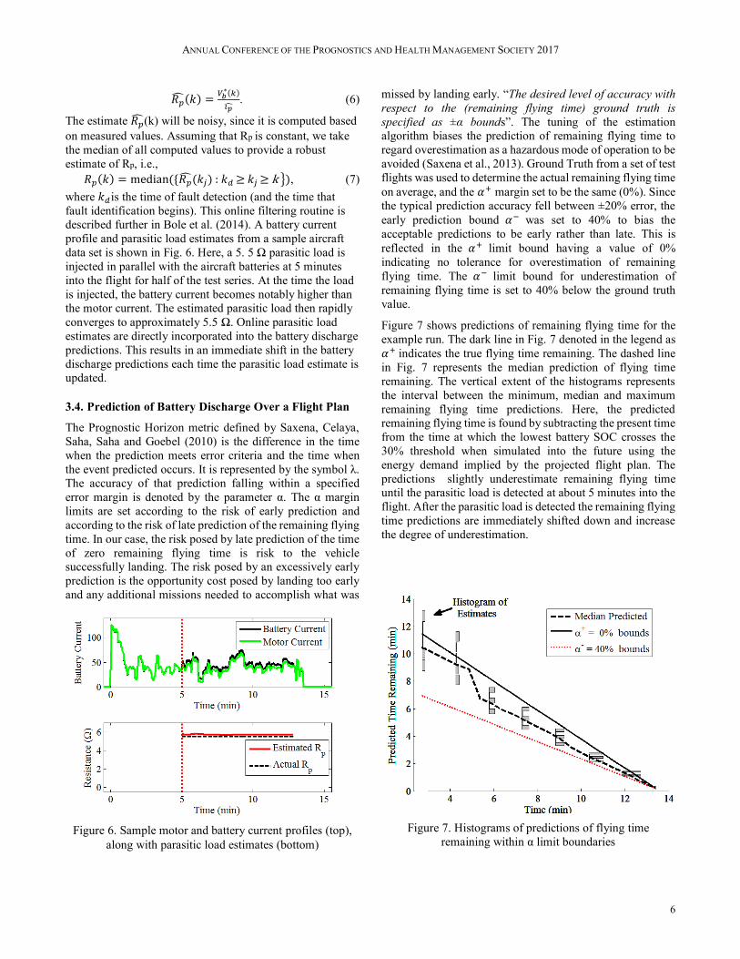
described further in Bole et al. (2014). A battery current

profile and parasitic load estimates from a sample aircraft

data set is shown in Fig. 6. Here, a 5. 5 Ω parasitic load is

injected in parallel with the aircraft batteries at 5 minutes

into the flight for half of the test series. At the time the load

is injected, the battery current becomes notably higher than

the motor current. The estimated parasitic load then rapidly

converges to approximately 5.5 Ω. Online parasitic load

estimates are directly incorporated into the battery discharge

predictions. This results in an immediate shift in the battery

discharge predictions each time the parasitic load estimate is

updated.

3.4. Prediction of Battery Discharge Over a Flight Plan

The Prognostic Horizon metric defined by Saxena, Celaya,

Saha, Saha and Goebel (2010) is the difference in the time

when the prediction meets error criteria and the time when

the event predicted occurs. It is represented by the symbol λ.

The accuracy of that prediction falling within a specified

error margin is denoted by the parameter α. The α margin

limits are set according to the risk of early prediction and

according to the risk of late prediction of the remaining flying

time. In our case, the risk posed by late prediction of the time

of zero remaining flying time is risk to the vehicle

successfully landing. The risk posed by an excessively early

prediction is the opportunity cost posed by landing too early

and any additional missions needed to accomplish what was

missed by landing early. “The desired level of accuracy with

respect to the (remaining flying time) ground truth is

specified as ±α bounds”. The tuning of the estimation

algorithm biases the prediction of remaining flying time to

regard overestimation as a hazardous mode of operation to be

avoided (Saxena et al., 2013). Ground Truth from a set of test

flights was used to determine the actual remaining flying time

on average, and the 𝛼+ margin set to be the same (0%). Since

the typical prediction accuracy fell between ±20% error, the

early prediction bound 𝛼− was set to 40% to bias the

acceptable predictions to be early rather than late. This is

reflected in the 𝛼+ limit bound having a value of 0%

indicating no tolerance for overestimation of remaining

flying time. The 𝛼− limit bound for underestimation of

remaining flying time is set to 40% below the ground truth

value.

Figure 7 shows predictions of remaining flying time for the

example run. The dark line in Fig. 7 denoted in the legend as

𝛼+ indicates the true flying time remaining. The dashed line

in Fig. 7 represents the median prediction of flying time

remaining. The vertical extent of the histograms represents

the interval between the minimum, median and maximum

remaining flying time predictions. Here, the predicted

remaining flying time is found by subtracting the present time

from the time at which the lowest battery SOC crosses the

30% threshold when simulated into the future using the

energy demand implied by the projected flight plan. The

predictions slightly underestimate remaining flying time

until the parasitic load is detected at about 5 minutes into the

flight. After the parasitic load is detected the remaining flying

time predictions are immediately shifted down and increase

the degree of underestimation.

Figure 6. Sample motor and battery current profiles (top),

along with parasitic load estimates (bottom)

Figure 7. Histograms of predictions of flying time

remaining within α limit boundaries


7

4. FLIGHT TEST VERIFICATION OF REMAINING FLYING

TIME PREDICTION

A description of the flight test experiment, followed by the

performance requirements, the β metric, the SOC ground

truth, SOC and remaining flying time results are found in this

section.

The flight test verification of the Edge 540T hardware and

software was initiated by loading the Cmax and Rs parameters

for the batteries used when the onboard battery management

software was started. The propulsion batteries were

previously characterized by a slow discharge laboratory

procedure, and then fitted to the equivalent circuit model

using the Nelder-Mead method. More details are found in

Bole et al., (2014).

4.1. Description of the Flight Experiment

A flight plan of timed airspeed segments at a fixed altitude

(described in section 3.2) was also loaded into the onboard

software. Only manual (stick-to-surface) pilot control

commands were used to perform the test flights for this

experiment. Aircraft propeller RPM, estimated battery SOC,

and predictions of remaining flying time were displayed on a

ground station display for the system operators in near real-

time. The motor throttle was controlled by the pilot to attain

each requested flight plan airspeed target. A second ground

station operator called out the actual airspeed achieved and

altitude as feedback to the pilot. The pilot adjusted the

vehicle’s airspeed to maintain the flight plan airspeed target

values for the flight plan segment time duration as described

in Section 3.2. These airspeed targets were all planned for

constant altitude flight plan segments. An “Amber Warning”

alarm was raised when the remaining flying time prediction

came within two minutes of the 30% SOC landing limit

threshold for the weakest battery. At the 2-minute “Amber

Warning”, the pilot was instructed to descend to landing

approach pattern altitude and to be ready to begin the landing

approach when the ground station displayed the “red alert”.

This indicated the lowest battery was at or below the 30%

SOC limit threshold or that a low voltage (17.0V) safety limit

threshold had been breached. The amber and red alerts are

depicted in Fig. 8. Once the “red alert” threshold alarm was

raised, an “End Research, Load Off” advisory status call was

made to the pilot. The pilot then began the landing approach

sequence and disarmed the parasitic load resistor bank. This

precaution was necessary because the resistor bank generates

sufficient heat to be a fire risk after several minutes without

the cooling from the relative air movement of flight. Once

landed, the motor was stopped and the vehicle was retrieved

by ground personnel to prevent any additional battery

consumption by ground taxiing. The battery data logging was

continued for an additional twenty minutes after landing to

document the recovery of the battery voltage that had been

depressed due to the power demand to sustain flight. This

battery voltage at near-equilibrium was used to compute an

empirical approximation of the ending battery SOC based

upon laboratory tests done at near-equilibrium (Bole et al.,

2013). The data logging during the experimental flights was

performed by the data system described in (Hogge et al.,

2011).

4.2. Performance Requirements

The specification of performance requirements for

verification of the remaining flying time predictions is

described next. The predictive element tested is an alarm that

warns system operators when the powertrain batteries are two

minutes from reaching 30% SOC under normal operations.

Accuracy requirements for the two minute warning were

specified as:

1. The prognostic algorithm shall raise an alarm no later

than two minutes before the lowest battery SOC estimate

falls below 30% for at least 90% of verification trial

runs.

2. The prognostic algorithm shall raise an alarm no earlier

than three minutes before the lowest battery SOC

estimate falls below 30% for at least 90% of verification

trial runs.

3. There should be enough charge present in the batteries

so as to complete at least 2 go-arounds in case of a

missed landing.

Here, the two minute alarm is biased to occur early rather

than late since the landing becomes unsafe if not enough

battery charge is present. The early alarm prediction bound

limits the “opportunity cost” of unnecessarily denied flying

time.

4. Required confidence to specify when prognosis is

sufficiently good – β > 50%

An additional requirement for the flying time prediction

verification specifies maximum bounds on the ending SOC

estimation error:

5. The ending SOC estimation error as identified from the

resting battery voltage must be less than 5% for at least

90% of verification trial runs.

4.3. β Metric of Prediction Performance

Prognostic algorithms inherently contain uncertainties and

often estimate the uncertainties in the predicted quantity.

These estimates can be used to infer the variability (spread)

in predictions. Figure 9 after Saxena et al. (2012) illustrates

the β metric of the fraction of the probability mass falling

between the two α bounds of acceptance. The higher the

value of β, the higher the confidence that a prediction will

remain within the two α bounds of acceptance. In Fig. 7 the


8

portion enclosed between the α limits is the β percentage of

the probability density function (PDF) contained between the

limits. In this example β is 86%, or 86% of the PDF is within

the α limits. The remaining portion outside the limits is

referred to as 𝛽+. A threshold criteria of 50% for the β metric

for the prediction to be acceptable for decision making was

proposed by Saxena, Roychoudhury, Celaya, Saha, Saha, and

Goebel (2012). We use 50% for this test series.

Referring back to Fig. 7 the β values based upon histogram

location before the parasitic load is engaged at time of 5

minutes are somewhat more than 50%. After the 5.0 minute

time index, the histograms show that all the β density is

contained within the α-bounds. The lower 50% bound on β works in conjunction with the α-bounds to specify

performance constraints. As the α-bounds get narrower (i.e.

less error tolerated) the probability density functions are

required to contain the spread in order to satisfy the same β criterion. Figure 8 shows how the α error bounds narrow and

the β histograms narrow as the 30% SOC threshold is

approached. In the example shown here, the two-minute

warning β histograms are all within the α bound limits

implying a β of 100%. Referring back to Fig. 7 the prognostic

horizon is somewhere before the beginning of the plot for the

sample flight since even when the upper limit of the first few

vertical bars is past the 𝛼+ limit, the included portion is still

greater than 50%. Figure 10 shows a cumulative plot of all

the β values from 15 flight tests with the 50% pass/fail

threshold dashed line. The flight that had a late prediction of

the two-minute warning coincided with a β of less than 50%.

In this run, the airspeed exceeded the target airspeed by as

much as 17% due to the pilot’s compensation for unsteady

winds aloft and the desire to provide a larger margin above

aircraft stall speed. The flight plan airspeed values were also

not adjusted for this change in keeping with the experiment

plan. An operator could want a β-derived status indicator that

would indicate if the flying time predictions are reliable.

However, since the β metric is calculated from the α bounds

which is in turn based upon the ground truth time of the

lowest battery crossing the 30% SOC threshold limit, and the

ground truth SOC is calculated from a measurement taken 15

minutes after the landing, it is not available online and can

only be computed offline well after the flight.

4.4. SOC Ground Truth

The definition of requirements 1, 2, and 4 stated previously

in section 4.2 use the term “SOC estimate”. The UKF state

estimation algorithm described earlier, is relied upon to

provide online estimates of battery SOC from measured

battery current and voltages. A more direct measurement of

battery SOC can be obtained after the experimental flight is

complete by allowing the batteries to rest until the terminal

voltage settles to a constant value. There is a known

relationship between the equilibrium battery voltage and the

SOC that can then be used to compute the ending SOC for all

Figure 9. β Probability Density Function area within α

acceptance limits.

Figure 8. Advisory alarms with β PDF histograms of

predictions

Figure 10. Passing β values for 15 flights


9

the powertrain batteries. The difference between the

estimated battery SOC at the end of each flight and the

measurement of SOC that is computed from the resting

battery voltage is referred to here as the ending SOC

estimation error. The allowed estimation error is specified in

requirement five.

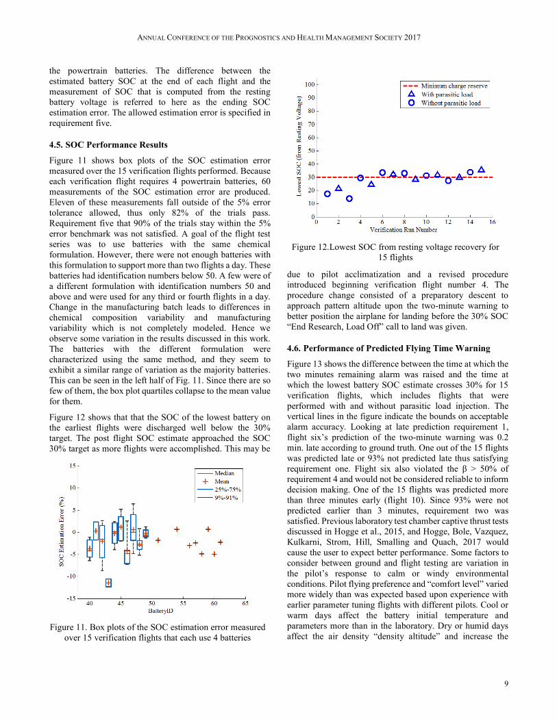
4.5. SOC Performance Results

Figure 11 shows box plots of the SOC estimation error

measured over the 15 verification flights performed. Because

each verification flight requires 4 powertrain batteries, 60

measurements of the SOC estimation error are produced.

Eleven of these measurements fall outside of the 5% error

tolerance allowed, thus only 82% of the trials pass.

Requirement five that 90% of the trials stay within the 5%

error benchmark was not satisfied. A goal of the flight test

series was to use batteries with the same chemical

formulation. However, there were not enough batteries with

this formulation to support more than two flights a day. These

batteries had identification numbers below 50. A few were of

a different formulation with identification numbers 50 and

above and were used for any third or fourth flights in a day.

Change in the manufacturing batch leads to differences in

chemical composition variability and manufacturing

variability which is not completely modeled. Hence we

observe some variation in the results discussed in this work.

The batteries with the different formulation were

characterized using the same method, and they seem to

exhibit a similar range of variation as the majority batteries.

This can be seen in the left half of Fig. 11. Since there are so

few of them, the box plot quartiles collapse to the mean value

for them.

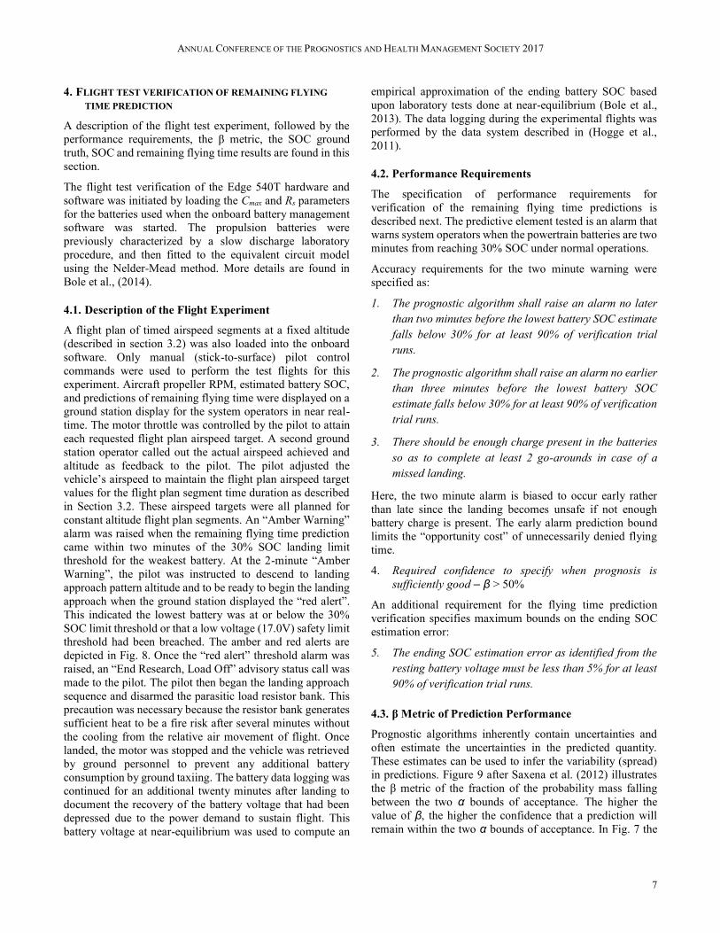
Figure 12 shows that that the SOC of the lowest battery on

the earliest flights were discharged well below the 30%

target. The post flight SOC estimate approached the SOC

30% target as more flights were accomplished. This may be

due to pilot acclimatization and a revised procedure

introduced beginning verification flight number 4. The

procedure change consisted of a preparatory descent to

approach pattern altitude upon the two-minute warning to

better position the airplane for landing before the 30% SOC

“End Research, Load Off” call to land was given.

4.6. Performance of Predicted Flying Time Warning

Figure 13 shows the difference between the time at which the

two minutes remaining alarm was raised and the time at

which the lowest battery SOC estimate crosses 30% for 15

verification flights, which includes flights that were

performed with and without parasitic load injection. The

vertical lines in the figure indicate the bounds on acceptable

alarm accuracy. Looking at late prediction requirement 1,

flight six’s prediction of the two-minute warning was 0.2

min. late according to ground truth. One out of the 15 flights

was predicted late or 93% not predicted late thus satisfying

requirement one. Flight six also violated the β > 50% of

requirement 4 and would not be considered reliable to inform

decision making. One of the 15 flights was predicted more

than three minutes early (flight 10). Since 93% were not

predicted earlier than 3 minutes, requirement two was

satisfied. Previous laboratory test chamber captive thrust tests

discussed in Hogge et al., 2015, and Hogge, Bole, Vazquez,

Kulkarni, Strom, Hill, Smalling and Quach, 2017 would

cause the user to expect better performance. Some factors to

consider between ground and flight testing are variation in

the pilot’s response to calm or windy environmental

conditions. Pilot flying preference and “comfort level” varied

more widely than was expected based upon experience with

earlier parameter tuning flights with different pilots. Cool or

warm days affect the battery initial temperature and

parameters more than in the laboratory. Dry or humid days

affect the air density “density altitude” and increase the

Figure 11. Box plots of the SOC estimation error measured

over 15 verification flights that each use 4 batteries

Figure 12.Lowest SOC from resting voltage recovery for

15 flights


10

energy demand necessary to maintain altitude. These sources

of variation are not present in the laboratory tests.

Another question to be considered is how well do the

repeated trials of the two-minute alarm indicate what we

should expect for future flights? An Anderson-Darling test

was run on the 15-flight data set of the two-minute warnings

to test if the alarm times came from a Gaussian distribution.

The test indicated that the alarm time predictions came from

a normal distribution at the 5% significance level. Since the

distribution is normal, a confidence interval test would be

valid. The standard error of estimate of the two-minute alarm

time given the sample mean is shown in Fig. 14. This figure

repeats Fig. 13 except that the statistical measures are

emphasized. The sample mean of the fifteen flights shows 2.6

minutes as the actual amber warning time as opposed to the

specified range of 2 to 3 minutes for the 2-minute flying time

remaining. The 95% confidence limits come from

adding/subtracting two “standard error of estimate” values

to/from the mean (Spiegel & Stephens, 1998). The numerical

value for the standard error of estimate was 0.39 for this data

set. The 95% confidence limits are biased to the early

prediction side of the 2 to 3 minute alarm specification shown

in the red dashed lines. This is to trade the opportunity cost

of missed possible flying time against not having enough

energy to repeat failed landing attempts. This trade-off was

made empirically at the end of the series of flight tests since

the initial tuning was based on captive-flight ground tests.

5. CONCLUSION

Flight tests to verify the performance of remaining flying

time predictions for a small electric aircraft were described.

Continued flight after aircraft battery packs have reached

30% SOC was defined as high risk operation for our

experimental vehicle, and are to be avoided if possible. The

flight tests did not pass the 5% ending SOC estimation error

requirement but were not far from meeting that requirement

(82% of 90%). The requirement that the two-minute warning

alarm be satisfied 90% of the time was satisfied 93% of the

time. Environmental and pilot variation are possible

confounding factors and need to be better accounted for with

an improved method. Repeatable testing such as that

described in this paper is necessary to effectively debug, tune,

and build trust in prognostic algorithms prior to deployment

in mission critical applications.

ACKNOWLEDGEMENT

This work was funded by the NASA Shadow Mode

Assessment using Realistic Technologies for the National

Airspace System (SMART NAS) Program of the Aeronautics

Research Mission Directorate (ARMD). Use of the Wireless

Intelligent Sensing Electromagnetic Environmental Effects

Research test chamber was appreciated. Allan White and

Kenneth Eure are thanked for helpful suggestions and

comments. Patrick Tae is thanked for his contribution to the

testing of the parasitic load apparatus as part of his intern

assignment. Samuel Bibelhauser is thanked for his

contribution of a test chamber data logger used for ground

tests as part of his intern assignment.

REFERENCES

Bole, B., Daigle, M., Gorospe, G.,. (2014). Online prediction

of battery discharge and estimation of parasitic loads for

an electric aircraft. European Conference of the

Prognostics and Health Management Society.

Bole, B., Teubert, C., Quach, C., Hogge, E., Vazquez, S.,

Goebel, K., & Vachtsevanos, G. (2013). SIL/HIL

replication of electric aircraft powertrain dynamics and

inner-loop control for V&V of system health

management routines. Annual Conference of the

Prognostics and Health Management Society.

Figure 13. Two-minute alarms for 15 flights

Figure 14. Two-minute alarms, 95% confidence limits


11

Ceraolo, M. (2000, November). New dynamical models of

lead-acid batteries. IEEE Transactions of Power

Systems, 15(4), 1184-1190.

Chen, M., & Rincon-Mora, G.A. (2006, June). Accurate

electrical battery model capable of predicting runtime

and I-V performance. IEEE Transactions on Energy

Conversion. 21(2), 504-511.

Daigle, M., Saxena A. & Goebel, K. (2012). An efficient

deterministic approach to model-based prediction

uncertainty estimation. Annual Conference of the

Prognostics and Health Management Society, 2012.

Ely, J., Koppen, S., Nguyen, T., Dudley, K., Szatkowski, G.,

Quach, C., Vazquez, S., Mielnik, J., Hogge, E., Hill, B.

& Strom, T. (2011). “Radiated Emissions From a

Remote-Controlled Airplane - Measured in a

Reverberation Chamber “. NASA/TM-2011-217146.

Hogge, E., Bole, B., Vazquez, S., Celaya, J., Strom, T., Hill,

B., Smalling, K. & Quach, C. (2015). Verification of a

remaining flying time prediction system for small

electric aircraft. Annual Conference of the Prognostics

and Health Management Society 2015.

Hogge, E., Bole, B., Vazquez, S., Kulkarni, C., Strom, T.,

Hill, B., Smalling, K., & Quach, C. (2017). Verification

of prognostic algorithms to predict remaining flying time

for electric unmanned vehicles. to appear in

International Journal of Prognostics and Health

Management, Vol. 8 doi: 2017

Hogge, E., Quach, C., Vazquez, S. & Hill, B. (2011). "A Data

System for a Rapid Evaluation Class of Subscale Aerial

Vehicle”. NASA/TM-2011-217145.

Julier, S. & Uhlmann, J. K. (1997). A new extension of the

Kalman filter to nonlinear systems. In Proceedings of the

11th international symposium on aerospace/defense

sensing, simulation, and controls (pp. 182-193)

Julier, S. & Uhlmann, J. (2004, March). Unscented filtering

and nonlinear estimation. Proceedings of the IEEE,

92(3), 401-422.

Nelder, J. & Mead, R. (1965). A simplex method for function

minimization. Computer Journal 1965; 7 (4), 308-313.

Quach, C., Bole, B., Hogge, E., Vazquez, S., Daigle, M.,

Celaya, J., Weber, A. & Goebel, K. (2013). Battery

charge depletion prediction on an electric aircraft.

Annual Conference of the Prognostics and Health

Management Society 2013.

Saha, B., Koshimoto, E., Quach, C., Hogge, E., Strom, T.,

Hill, B., Vasquez, S. & Goebel, K. (2011). Battery health

management system for electric UAV’s. IEEE

Aerospace Conference. Big Sky, MT.

Saha, B., Quach, C. & Goebel, K. (2012). Optimizing battery

life for electric UAVs using a Bayesian framework. 2012

IEEE Aerospace Conference.

Saxena, A., Celaya, J., Saha, B., Saha, S. & Goebel, K.

(2010). Metrics for offline evaluation of prognostic

performance. International Journal of Prognostics and

Health Management, Vol. 1(1) 001, pp 13-15, doi: 2010

Saxena, A., Roychoudhury, I., Celaya, J., Saha, B., Saha, S.

& Goebel, K. (2012). Requirements flowdown for

prognostics and health management.

Infotech@Aerospace Conference (pp. 8-9). Garden

Grove, CA: AIAA, Reston, VA.

Saxena, A., Roychoudhury, I., Lin, W. & Goebel, K. (2013).

Towards requirements in systems engineering for

aerospace IVHM design. AIAA Conference, 2013.

AIAA, Reston, VA.

Spiegel, M. R. & Stephens, L. J., (1998). Schaum’s outline of

theory and problems of statistics. New York, NY:

McGraw-Hill.

Zang, H., & Chow, M.-Y., (2010). Comprehensive dynamic

battery modeling for PHEV applications. In IEEE

power and energy society general meeting.

BIOGRAPHIES

Edward F. Hogge received a B.S. in

Physics from the College of William and

Mary in 1977. He has provided engineering

services to the government and currently is

employed by Northrop Grumman

Technology Services. He has recently been

supporting aviation safety research through

the implementation of electronic systems for subscale

remotely piloted aircraft and through commercial aircraft

simulation. He is a member of the American Institute of

Aeronautics and Astronautics.

Chetan S. Kulkarni received the B.E.

(Bachelor of Engineering) degree in

Electronics and Electrical Engineering from

University of Pune, India in 2002 and the

M.S. and Ph.D. degrees in Electrical

Engineering from Vanderbilt University,

Nashville, TN, in 2009 and 2013,

respectively. He was a Senior Project Engineer with

Honeywell Automation India Limited (HAIL) from 2003 till

April 2006. From May 2006 to August 2007 he was a

Research Fellow at the Indian Institute of Technology (IIT)

Bombay with the Department of Electrical Engineering.

From Aug 2007 to Dec 2012, he was a Graduate Research

Assistant with the Institute for Software Integrated Systems

and Department of Electrical Engineering and Computer

Science, Vanderbilt University, Nashville, TN. Since Jan

2013 he has been a Staff Researcher with SGT Inc. at the

Prognostics Center of Excellence, NASA Ames Research

Center. His current research interests include physics-based

modeling, model-based diagnosis and prognosis. Dr.

Kulkarni is a member of the Prognostics and Health

Management (PHM) Society, AIAA and the IEEE.


12

Sixto L. Vazquez Mr. Vazquez obtained

MSEE from Old Dominion University in

1990 and BSEE from the University of

Puerto Rico in 1983. He has developed real-

time 3D graphical simulations to aid in the

visualization and analysis of complex

sensory data. He has developed techniques

to interactively process, analyze, and integrate sensory data

from multiple complex, state-of-the-art sensing technologies,

i.e. FMCW Coherent Laser Radar range measuring system,

Bragg grating Fiber Optic Strain Sensing system, etc., into

simulation. In recent years, he has developed software for the

Ardupilot and associated ground station.

Kyle M. Smalling Kyle Smalling obtained

his B.S. in Aerospace Engineering from Cal

Poly Pomona in 2013. He is an avid remote

control vehicle enthusiast both personally

and professionally. His areas of research

include Health Prognostics and developing

Safety Critical hardware and software. He is

employed by Northrop Grumman Technology Services.

Thomas H. Strom was born in Aberdeen,

WA, 1924. He graduated from Hoquiam

High School in 1942, and attended Seattle

University and the University of

Washington 1953-1960. He served in the

U.S. Navy during World War II as a Radar

Technician. He was an employee of the Boeing Corp. Wind

Tunnel, Seattle, WA 1947-1972. He was Senior Engineer

with principal expertise in flutter and aeroelastic wind tunnel

modeling. He was the founder and president of Dynamic

Engineering, Inc., Newport News, VA, until 1987. He has

served as a consultant to the Aeroelasticity Group of NASA

Langley Research Center (LaRC) and continues to provide

engineering and technical services to LaRC through Northrop

Grumman Technology Services.

Cuong C. Quach received his M.S. from the

School of Physics and Computer Sciences at

Christopher Newport University in 1997. He

is a staff researcher in the Safety Critical

Avionics Systems Branch at NASA Langley

Research Center. His research areas include

development and testing of software for

airframe diagnosis and strategic flight path conflict detection.

flight tests of a remaining flying time prediction system

Documents