1  

Remaining Useful Life Prediction of Individual Units Subject to Hard Failure

QIANG ZHOU1*, JUNBO SON2, SHIYU ZHOU2, XIAOFENG MAO3, MUTASIM SALMAN3

1 Department of Systems Engineering and Engineering Management, City University of Hong Kong, Kowloon, Hong Kong E-mail: q.zhou@cityu.edu.hk 2 Department of Industrial and Systems Engineering, University of Wisconsin-Madison, WI 53706, USA 3 General Motors Research & Development, Warren, MI, USA

Abstract

To develop a cost-effective condition-based maintenance strategy, accurate prediction of remaining useful

life (RUL) is the key. It is known that many failure mechanisms in engineering can be traced back to

some underlying degradation processes. In this paper, we propose a two-stage prognostic framework for

individual units subject to hard failure, based on joint modeling of degradation signal and time-to-event

data. The proposed algorithm features low computational load, online prediction and dynamic updating.

Its application to automotive battery RUL prediction has been discussed in this paper as an example. The

effectiveness of the proposed method has been demonstrated through both simulation study and real data.

Keywords: Remaining useful life prediction, hard failure, joint model

1. Introduction

In engineering applications, the reliability of a critical unit is crucial to guarantee the overall functional

capabilities of the entire system. Failure of such a unit can be catastrophic. Turbine engines of airplanes,

power supplies of computers, and batteries of automobiles are typical examples where failure of the unit

would lead to breakdown of the entire system. For these reasons, such critical units must be well-

maintained for the overall system reliability and to improve end user satisfaction. In traditional

maintenance strategies, unit is either repaired after its failure (run-to-failure maintenance) or scheduled

for time-based preventive maintenance (planned maintenance). In recent years, a more cost-effective

                                                            * Corresponding author

2  

strategy called condition-based-maintenance (CBM) (Jardine, Lin, and Banjevic (2006); Ye, Shen, and

Xie (2012)) has been proposed. The rationale supporting this procedure is that many system failure

mechanisms can be traced back to some underlying degradation processes. RUL prediction can be made

based on degradation signal collected. The degradation signal should be strongly associated with the

failure of the unit and contains important information about its health status. As the prediction is

preferably to be made online for units working in the field, a prognostic algorithm featuring real-time

prediction with a low computational requirement is desirable.

With the availability of degradation signal, RUL distribution is typically estimated based on modeling

the degradation signal hitting some pre-determined failure threshold (e.g., Lu and Meeker (1993); Gorjian

et al. (2009); Gebraeel (2006); Ye and Chen (2014)). These methods are called first-hitting-time (FHT)

models and the failure they are dealing with is called soft failure. However, hard failure, where the unit

keeps working until it breaks down, is also quite common in practice. The key difference is that the

degradation signals will normally exhibit different values at failure. In some applications, it is also

possible that a fixed failure threshold is hard to specify due to the following reasons: (1) the threshold

depends on the unit’s individual specific characteristics, which varies randomly from unit to unit due to

variation in their manufacturing process; (2) there are multiple potential failure mechanisms contributing

to the same degradation signal; (3) the failure threshold for the degradation signal is a ‘gray’ area. Non-

existence of a fixed failure threshold poses significant difficulties to FHT algorithms. Very limited

literature can be found in the engineering field dealing with the prognosis under hard failure (Liao et al.

(2006); Wang and Coit (2007); Yu and Fuh (2010)). On the other hand, time-to-event data about the

failure or censoring information may also be available besides degradation signal in many applications.

Time-to-event data contain useful information about life time distribution and has been extensively used

in traditional reliability engineering. In engineering field, however, these two types of data are rarely

analyzed together in an integrated fashion to extract the full information contained within both.

The integrated analysis of the degradation data and time-to-event data makes possible the prognosis

without a fixed failure threshold. Joint modeling of time-to-event data and degradation signal has been

3  

studied in the area of clinical trials, where it is common to collect time-to-event outcome together with

some repeated measurements of patients during the study. Comprehensive reviews of the related methods

in joint modeling can be found in Yu et al. (2004), and Tsiatis and Davidian (2004). The measurement,

often called ‘surrogate marker’ or ‘biomarker’ in the related literature, is strongly associated with the

death of the patient or recurrence of some disease and hence acts as a critical health indicator. Two mostly

well-known examples in the clinical study are CD4 lymphocyte count in AIDS (Tsiatis et al. (1995);

Bycott and taylor (1998); Wang and Taylor (2001)) and PSA level for early detection and recurrence of

prostate cancer (Pauler and Finkelstein (2002); Yu, Taylor, and Sandler (2008); Yu et al. (2004)). Under

the joint modeling framework, degradation signal is often modeled by mixed effects model (Laird and

Ware (1982)) and time-to-event data are modeled by the Cox proportional hazard (PH) model (Cox

(1972)). The surrogate marker is used as a time-dependent covariate in the Cox PH model so that changes

of the surrogate marker impacts the hazard rate. In this approach, the failure of a unit does not depend on

a specific threshold but is rather described probabilistically by the hazard function in the Cox PH model.

These unique advantages make it a suitable tool for RUL prediction in engineering applications

previously described. However, joint modeling in biostatistics has been predominantly focused on

studying the impact of covariates on the hazard rate of the population. Very few attempts have been made

to study its application in prognosis, particularly RUL prediction for individuals (Pauler and Finkelstein

(2002); Yu, Taylor, and Sandler (2008); Rizopoulos (2011)). Furthermore, the joint modeling framework

is computationally intensive, posing significant difficulties to its implementation in real-time online

prediction for engineering applications.

The joint model is an extension of the Cox PH model with an additional model for the degradation

signal. The model allows unit-to-unit variations of the degradation path by using the mixed effects model.

Traditionally, degradation signal can be simply incorporated into a Cox PH model as a time-dependent

covariate, but with notable difficulties in parameter estimation if observed signals are used directly (Yu et

al. (2004)). Cox PH model treats the observation as deterministic without random error, hence parameters

estimation is biased towards null and the amount of bias is proportional to the magnitude of the random

4  

error in the degradation signal (Prentice (1982)).

In this paper, we propose a prognostic framework for individual unit RUL prediction under hard

failure, based on the idea of joint modeling of the time-to-event data and degradation signal. In this

method, we assume historical records of a group of similar units are available for model fitting and

degradation signal of the unit to be predicted can be obtained. A two-stage approach, containing an offline

modeling stage based on the database and an online prediction stage based on the individual unit’s

degradation signal, has been proposed. The proposed model allows continuous updating of the failure

distribution based on the observed signal from the in-service unit. The model updating can be done by a

closed-form Bayesian formula, thus the computational burden can be significantly reduced. The method’s

low computation at the online stage makes it possible to be implemented in the field. For example,

automotive engineers are interested in the online prediction of automotive battery RUL, which impacts

customer satisfaction and warranty cost to the company. A vital health indicator of the automotive battery

is its internal resistance which can be estimated based on engine cranking signal through an ohmic

relationship (Zhang et al. (2011)) or through more complicated algorithms such as the fractional order

model discussed by Cugnet et al. (2010). The proposed prognostic algorithm has a low requirement on

computation so that it has the potential to be implemented in vehicle onboard micro-controllers.

The rest of this paper is organized as follows. The problem formulation and a detailed description of

the proposed method are given in Section II. Section III presents a simulation study where the

effectiveness of the proposed method is demonstrated. Section IV applies the method to real data from a

battery aging test. Finally, Section V concludes the paper and discusses some possible future work.

2. Prediction on RUL

2.1. The prognostic framework

The proposed prognostic framework is composed of two stages: the offline modeling stage, and the

online prediction stage. During the offline stage, parameters of the prognostic model are estimated based

on a historical database that contains event times, time-stamped degradation signal and possibly some

other time-fixed covariates (such as manufacturer, device type, etc.) for a number of similar units. During

5  

the online stage, degradation signal of an in-service unit is obtained and used for prediction of the unit’s

RUL based on the model parameters estimated during the offline stage. The predictions made for an in-

service unit can be updated as more measurements on the degradation signal are obtained during its usage.

Regarding the computational load for the algorithm, there is no stringent requirement for the offline

stage as it only has to run once to estimate the population parameters when building the prognostic model,

or once in a while when data collected from additional units are added to the database and updated

parameter estimates are desired. However, it is desirable to keep the computational load at a low level for

the online stage.

2.2. Modeling

Assume the database contains historical data of N similar units, which can be viewed as a random

sample from the same underlying population. For the ith unit, its associated data is denoted as

{ , , , }hi i i i iD V r w , where Vi = min(Ti, Ci) is the event time (the unit either failed at time Ti or was

censored at time Ci without knowing its actual time of failure), i is an event indicator corresponds to the

type of the event (i = 1/0 indicates the unit has failed/censored),

1 2 1 2{ , ,..., } { ( ), ( ),..., ( )}i i

h T Ti i i in i i i i i inr r r r t r t r t r is the history of observed degradation signal (e.g.,

internal resistance of a battery) with iin it V , and the vector iw contains all the other time-fixed

covariates that are associated with the unit. Note that the time components in the dataset are not absolute

times measured in calendar date but relative time lengths starting from the moment when the unit came

into service. Based on the nature of data { , , , }hi i i i iD V r w , the modeling approach involves two distinct

sub-modeling approaches: longitudinal analysis for the degradation signal and survival analysis for the

time-to-event data.

2.2.1. Sub-model I: Longitudinal analysis for the degradation signal

In this section, the degradation path of the signal will be modeled through random effects model, by

assuming the degradation process follows some parametric path. Degradation signal provides important

6  

information as the health status of a unit and hence modeling of its evolution will facilitate the prognosis

of its RUL. The random coefficients in the model are particularly suitable for describing the variations

among a population of similar units.

Without loss of generality, we assume the degradation signal increases as the unit degrades (e.g., a

battery’s resistance increases as it ages). The degradation path of the ith unit is assumed to follow the

model:

( ) ( ) ( ) ( ) ( )Ti i i i ir t x t t t t z b , (1)

where ( )ix t is the true but unobservable value of the degradation signal, ( )i t is the measurement error

which is assumed to be independent and follows normal distribution N(0, σ2), ( )T tz contains the intercept

and time-dependent regression functions and bi is a vector of random coefficients. With the random

coefficients, model (1) assumes those units have distinct but similar degradation paths.

In cases where nonlinear behaviors of degradation signal are evident, we may add higher order

polynomial terms or splines in ( )T tz . We may also include certain specific nonlinear functions of time

(e.g., log(t) or t0.5) in the model, if they are believed to be the correct forms based on either physical

knowledge or empirical results. However, identifying a single best growth model that works for all

applications is impossible and hard to justify. ( )T tz is a user-defined function requiring domain

knowledge and experience of the specific system degradation process. It should be defined on a case by

case basis. Figure 1 shows an example of resistance measurements of 10 lead acid batteries during an

accelerated aging test on their engine cranking capability. From the motivating data and the dataset

illustrated in Figure 7, we have found that the quadratic form would be appropriate to describe the

degradation signal propagation for the particular application of automotive lead-acid batteries. The

quadratic structure or polynomial in general, has been commonly used in the prognosis literature for

individual components (Gebraeel (2006); Gebraeel et al. (2005); Elwany, A. et al. (2009)). The

polynomial model can also be transformed to handle the exponential or the power form (Gebraeel et al.

7  

(2005)).

For the random effects, we assume ib follows a multivariate normal distribution ( , )b bN , possibly

after some transformation of the signal. Studies conducted by Rizopoulos and Verbeke (2008), and Hsieh,

Tseng, and Wang (2006) show the model parameter estimates are rather robust to misspecification of the

random effects distribution, particularly as the number of measurements per unit increases. Note that the

time points when measurements are made may be different for various units: for the ith unit, its

degradation signal was measured at times: ti1, ti2,…, tini.

Figure 1. Resistances of 10 lead acid batteries during an accelerated aging test

2.2.2. Sub-model II: Survival analysis for time-to-event data

In this section, we model the time-to-event data (Vi , i ) based on time-fixed covariates wi and time-

dependent covariates ( )ix t from the degradation model previously described. Typically, ( )ix t would be

associated with a single coefficient to reflect its impact on the hazard rate. For greater flexibility, we split

( )ix t into two components, its initial value (0)ix and its increase ( ) (0)i ix t x , and associate them with

two different coefficients. This allows the two components to have different impacts on the hazard rate, a

phenomenon we have observed in the application of automotive batteries. By expressing

1( ) [1, ( )]T Tt tz z and 0 1[ , ]T T

i i ibb b , we have assumed the following form for hazard rate of the ith unit:

0 0 0 1 1 1( ) ( )exp[ ( ) ]T Ti i i ih t h t b t w z b , (2)

where h0(t) is the baseline hazard rate, is a vector of association parameters linking fixed covariate(s)

8  

in wi with the hazard rate, 0 and 1 are the parameters linking the degradation signal initial value and its

increase with the hazard rate, respectively. If imposing the constraint 0 = 1, (2) will reduce to the typical

formulation where the entire degradation signal ( )ix t is associated with a single parameter . Basically,

the degradation signal is included as a factor for the hazard rate function. Factors that impact the lifetime

of units manifest themselves through the degradation signal. Thus, the degradation signal value gives us a

good idea of the unobservable health status of the unit.

Note h0(t), , 0 and 1 do not depend on i; they represent population characteristics while individual

specific information is contained in wi and bi. The baseline hazard rate h0(t) can be assumed to have some

parametric forms such as Weibull, or some step function, but can also be nonparametric for better

flexibility. The two sub-models, (1) and (2), share the same random effects bi and are conditionally

independent given bi . We use 20 1{ , , , , , }b b to collectively denote all the parameters in the

two models.

It is worth pointing out the difference between the conventional Cox PH model and the joint model in

terms of prognosis. One simple extension from the Cox PH model would be having a simple regression

model for the degradation signal to predict its future value, e.g., zT(t)b. However, this would produce the

same prediction results for all future units (with the same wi). The joint model uses mixed effects model

to account for unit-to-unit variations by allowing b to be random, providing individualized prediction

results for each in-service unit.

2.3. Parameter estimation

In practice, Θ and h0(t) are unknown and need to be estimated based on the database information.

Based on the conditional independence, the observed data likelihood for the ith unit in the database is

(note ib is unobservable)

( , , , ; ) ( , , | , ; ) ( ; )

( , | , ; ) ( | ; ) ( ; )

h hi i i i i i i i i i i

hi i i i i i i i

p V p V p d

p V p p d

r w r w b b b

w b r b b b

, (3)

9  

where ( , | , ; )i i i ip V w b corresponds to the survival model and ( | ; )hi ip r b corresponds to the

degradation model. The three components in Equation (3) are:

0 0 0 1 1 1 0 0 0 1 1 10

( , | , ; ) [ ( | , ; )] ( | , ; )

( )exp[ ( ) ] exp ( )exp[ ( ) ]

i

ii

i i i i i i i i i i i i

VT T T Ti i i i i i i i

p V h V S V

h V b V h u b u du

w b w b w b

w z b w z b

, (4)

2

221 1

[ ( ) ]1 1( | ; ) [ | ; exp

22

i iTn n

ij ij ihi i ij i

j j

r tp p r

z b

r b b , (5)

and

1/2 1/2

1 1( ; ) exp

(2 ) | | 2T

i i b b i bkb

p

b b b

, (6)

where k is the number of parameters in ib . There are two ways for parameter estimation using the

likelihood functions defined in (4), (5) and (6). One is directly maximizing the joint log-likelihood

function defined as 1log ( , , , ; )

N hi i i ii

p V

r w and the other employs the EM algorithm by treating

ib as missing variable (Wulfsohn, M., and Tsiatis, A. (1997)). The joint likelihood function has a complex

form, making both methods computationally demanding. To alleviate the computational load, a “two-

stage” approximation method has been used frequently in the joint modeling literature (Tsiatis, Degruttola

and Wulfsohn (1995)). It estimates the parameters in the mixed effects model first, then estimates the

parameters in the Cox PH model by treating the mixed effects model as known. In this way, the mixed

effects model provide “true” values of the time-dependent covariate at any time point to facilitate the

estimation of the Cox PH model. Doing so will introduce some bias (Tsiatis, Degruttola and Wulfsohn

(1995); Bycott and Taylor (1998)). Fortunately, according to a comparison study between the EM

algorithm and the two-stage method, the difference is negligible (Wulfsohn and Tsiatis (1997)). For this

reason, the two-stage method is well-accepted in literature for its efficient computation with negligible

bias (Yu et al. (2004)). In the following sections, we let ̂ and 0̂( )h t denote the estimated parameters.

10  

2.4. Predicting the RUL of a new unit

Based on the model previously described and its estimated parameters, predictions can be made for the

RUL of a new in-service unit p during the online stage. This new unit is similar to those contained in the

database, and they can be considered as individuals sampled from the same population. We assume that

unit p is still in use and its degradation signal is obtained intermittently during its usage. As individual

specific information is contained within wp and bp (i.e., the time independent covariate and degradation

path coefficient of unit p), we need to estimate bp based on its degradation signal in order to make the

prediction (wp is normally known in practice). We use a Bayesian update scheme, where both the

population information contained in the database and the individual specific information contained in its

degradation signal can be blended together for estimation.

2.4.1. Bayesian estimation for unit p

At the time instant t* when the prediction is to be made, assume there are m values of degradation

signal available for unit p: Tpmppppp

Tpmppp trtrtrrrr )}(),...,(,)({},...,,{ 2121

* r , where *pmt t . The

degradation model for unit p is:

( ) ( ) ( ) ( ) ( )Tp p p p pr t x t t t t z b .

For convenience, we write the above equation in the following matrix form

***pppp EbZr ,

where *1 2[ ( ), ( ),..., ( )]T

p p p p p p pmt t t E is the m×1 error vector, and *pZ is an m×k matrix given as

below

1

2*

( )

( )

...

( )

Tp

Tp

p

Tpm

t

t

t

z

zZ

z .

The asterisk indicates the variables are dependent upon the time instant t*.

Specification of a prior in a Bayesian approach typically depends on the availability of closely related

11  

historical data and/or expert knowledge. In our case, it is natural to choose the prior based on the database

information as we consider the unit p and the database units are similar. Using the estimated distribution

of bi as the prior for bp, the posterior distribution of bp is

)()|()|( **ppppp pp bbrrb ,

where ˆˆ( ) ( , )p b bN b is the prior distribution of pb and )|( *ppp br is the likelihood function given as

2

2

12

1

*

ˆ

])([

2

1exp

ˆ2

1]ˆ;|[)|(

ppj

Tpj

m

j

m

jppjpp

trrpp

bzbbr Θ . (7)

It can be shown through straightforward derivation that the posterior distribution is also multivariate

normal. Assume )ˆ,ˆ()|( ***pppp Np Σμrb , we have

12**1*

12****

ˆ/)()ˆ(ˆ

ˆ)ˆ(ˆ/)(ˆˆ

pT

pbp

bbpT

ppp

ZZ

μrZμ

ΣΣ

ΣΣ.

Proof of the above result is given in the Appendix. This neat closed form update for the distribution of bp

allows the parameter estimation to be made with a low computation effort during online stage. Since we

use the two-stage estimation scheme, the *( | )p pp b r can be re-estimated, or updated, without considering

the ( , | , ; )i i i ip V w b . Thus, the overall computation for the online stage can be reduced significantly.

2.4.2. RUL prediction

Based on the previously estimated parameters, the RUL distribution of unit p can be made in the form

of its survival function conditional upon the fact that the unit survives no shorter than t*. Given bp, the

survival function is

*0

0

*0

0 0 0 1 1 1*

ˆˆ( | , , ; , ( ))

ˆˆ( | , ; , ( ))ˆˆ( | , ; , ( ))

ˆ ˆ ˆˆexp{ ( )exp[ ( ) ] }

p p

p p

p p

t T Tp p pt

S t t h t

S t h t

S t h t

h u b u du

w b

w b

w b

w z b

, (8)

12  

where *t t and the function equals to 1 if t = t*. Based on Equation (8) and the posterior distribution of

bp, the estimated survival function can be expressed in the form of a distribution and hence its

corresponding point-wise Bayesian credible interval.

In many cases, a point estimate of the survival function may be desirable in practice. Based on

Equation (8), the marginal survival function obtained by integrating out bp is

ppppppp dpthttSthttS brbbwrw )|())(ˆ,ˆ;,,|())(ˆ,ˆ;,,|( *0

*0

** ΘΘ . (9)

A special case for Equations (8) and (9) is when t* = 0, i.e., a newly installed unit without any

degradation signal available. In such case, we can use the prior distribution ( )p b instead of its posterior

distribution to make the prediction. As there is no individual specific information about the unit’s

degradation path, the prediction will only reflect the population average behavior extracted from the

database, adjusted for the time fixed covariate pw .

The evaluation of Equation (9) is computationally demanding due to the multiple integral which has no

closed form expression. Because )|( *ppp rb is a multivariate normal density function, this integral can be

approximated efficiently by using Gauss-Hermite quadrature.

First, we convert )|( *ppp rb to a standard multivariate normal distribution of the same dimension by

letting * *ˆp p pA b z , where *pA is a k×k square matrix from the decomposition * * *ˆ T

p p pA A and z

follows a k-dimensional multivariate standard normal distribution. The existence of *pA is guaranteed by

the fact that *ˆp is symmetric and positive definite. Define a k×1 vector 0 1 1

ˆ ˆ ˆ ( )T

Tz t z , we have

0 * *0 0 1 1 1 0 1 1

1

ˆ ˆ ˆ ˆ ˆ ˆ ˆ( ) ( ) ( )pT T T Tp p z p z p p

p

bb t t A

z b z b zb

. (10)

Based on Equations (9) and (10), the change of variable from pb to z gives us the following result:

13  

zzz

zzzAμβwγ

rw

dpG

dpduuh

thttSt

t ppTzp

T

pp

)()(

)(})]ˆ(ˆˆexp[)(ˆexp{

))(ˆ,ˆ;,,|(

*

**0

0**

Θ

. (11)

where p(z) is the probability density function of a k-dimensional standard multivariate normal distribution,

and G(z) is the remaining part of the integrand. The dependence of G(z) on other parameters is suppressed

here for simplicity. Based on Equation (11), we have the following approximation for the marginal

survival function:

s

i

s

iisisikikpp

k

kkcczzGthttS

1 1,,,,12/0

**

1

11...),...,(...

)2(

1))(ˆ,ˆ;,,|(ˆ

Θrw , (12)

where s is the number of nodes used, z’s are the zeros of sth order Hermite polynomial and c’s are their

associated weights. Since the survival function is typically smooth and well-behaved as long as N is not

too small, we can expect a good approximation with even a small s (e.g., s < 10 or even s < 5). The

evaluation of G(z) involves a simple integral over time t, which can be done very fast through either

Gauss-Legendre quadrature or any classical numerical integration method such as the Simpson’s method.

In Equation (12), G(z) needs to be evaluated sk times, which normally is not large since k, the dimension

of pb , is usually a small number.

We discuss an alternative estimating method for the marginal survival function that can be evaluated

even faster than Equation (12), particularly with large k value. It uses the expected value of the hazard

rate function and integrates it over time t. Specifically, since )|( *ppp rb is multivariate normal * *ˆˆ( , )p pN ,

11100 )(ˆˆˆ pT

ppT tb bzwγ follows a univariate normal distribution given as

)ˆˆˆ,ˆˆˆ(~)(ˆˆˆ **11100 zp

Tzp

Tzp

Tp

Tpp

T Ntb ββμβwγbzwγ Σ .

Hence, ])(ˆˆˆexp[ 11100 pT

ppT tb bzwγ follows a lognormal distribution and the expected value of

hazard rate function is

14  

]2/ˆˆˆˆˆˆexp[)(]|)(ˆ[ **0 zp

Tzp

Tzp

Tp ththE ββμβwγb Σ .

Therefore, we obtain an alternative estimator for the marginal survival function as

}]2/ˆˆˆˆˆˆexp[)(ˆexp{))(ˆ,ˆ;,,|(~

*

**00

** duuhthttSt

t zpTzp

Tzp

Tpp ββμβwγrw ΣΘ . (13)

This method is significantly faster than that based on Equation (12) as it primarily involves closed

form calculations except the simple integration over time t. Another major advantage of this method is

that the computational load does not increase much as k increases.

It should be pointed out that Equation (13) and Equation (9) are algebraically different. To compare

those two methods, let 0 0 0 1 1 1*

ˆ ˆ ˆˆ( ) ( ) exp[ ( ) ]t T T

p p p ptH h u b u du b w z b , we can then rewrite

Equation (9) as

)]}({exp[)|()](exp[

)|())(ˆ,ˆ;,,|())(ˆ,ˆ;,,|(

*

*0

*0

**

ppppp

ppppppp

HEdpH

dpthttSthttS

bbrbb

brbbwrw ΘΘ

,

and Equation (13) as

)]}([exp{))(ˆ,ˆ;,,|(~

0**

ppp HEthttS brw Θ .

As the exponential function is convex, the following relationship always holds per Jensen’s inequality

(Jensen (1906)):

))(ˆ,ˆ;,,|(~

)]}([exp{)]}({exp[))(ˆ,ˆ;,,|( 0**

0** thttSHEHEthttS pppppp ΘΘ rwbbrw . (14)

The above inequality describes the relationship between Equation (9) and Equation (13), subject to

numerical errors if approximations are used for the integrals. According to Inequality (14), the alternative

estimate of the marginal survival function can be viewed as a conservative estimator rather than an

approximated value: the predicted survival function yields smaller survival probability (e.g., shorter RUL

prediction). For critical components and/or risk adverse users, a conservative estimator may be preferred,

in addition to its computational advantage.

The proposed prognostic algorithm can update the RUL estimation as new measurements of the

15  

degradation signal of unit p become available. For example, if an updated prediction is to be made at a

time instant ** *t t when some additional measurements have become available, an updated posterior

distribution )|( **ppp rb of bp can be obtained and hence an updated estimation ))(ˆ,ˆ;,,|(ˆ

0**** thttS pp Θrw

for the survival function. This updating process is illustrated in Figure 2.

Figure 2. Updating scheme for survival function estimation

3. Simulation study

3.1. Demonstration of the joint prognostic framework

To demonstrate the effectiveness of the proposed algorithm, a simulation study is conducted. In the

study, data are generated in the form of { , , , }hi i i i iD V r w with N = 1000 artificial units as a database

for offline stage parameter estimation. A new unit p is then generated and its RUL predicted at some time

instant t* during its lifetime. Estimated results are compared with the true values for assessment of

prediction accuracy. Without loss of generality, in this study we assume the time unit is month, and the

degradation signal measurements are obtained regularly at each month. In this simulation study, we use

the Weibull baseline hazard rate function:

1 1.05 10( ) 0.001 1.05h t t t .

We assume the underlying true degradation path has the following form

1.2 1.70 1 2( ) ( ) ( ) ( )T

i i i i i i ir t t t b b t b t t z b , (15)

16  

where the distribution of bi in the simulation is set as ( , )b bN with

[2.5,0.01,0.01]

0.2 4 4 7 5

4 4 3 6 1 7

7 5 1 7 3 6

Tb

b

e e

e e e

e e e

, (16)

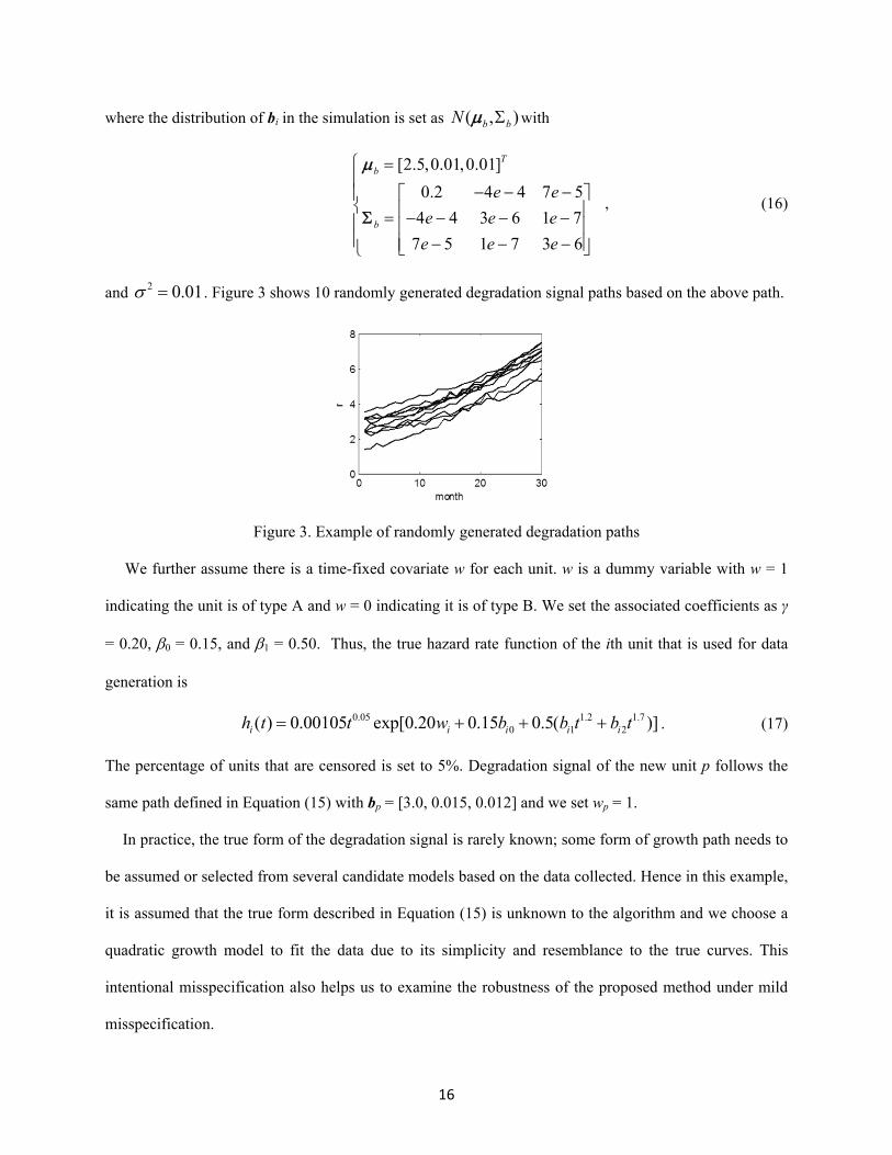
and 2 0.01 . Figure 3 shows 10 randomly generated degradation signal paths based on the above path.

Figure 3. Example of randomly generated degradation paths

We further assume there is a time-fixed covariate w for each unit. w is a dummy variable with w = 1

indicating the unit is of type A and w = 0 indicating it is of type B. We set the associated coefficients as γ

= 0.20, 0 = 0.15, and 1 = 0.50. Thus, the true hazard rate function of the ith unit that is used for data

generation is

0.05 1.2 1.70 1 2( ) 0.00105 exp[0.20 0.15 0.5( )]i i i i ih t t w b b t b t . (17)

The percentage of units that are censored is set to 5%. Degradation signal of the new unit p follows the

same path defined in Equation (15) with bp = [3.0, 0.015, 0.012] and we set wp = 1.

In practice, the true form of the degradation signal is rarely known; some form of growth path needs to

be assumed or selected from several candidate models based on the data collected. Hence in this example,

it is assumed that the true form described in Equation (15) is unknown to the algorithm and we choose a

quadratic growth model to fit the data due to its simplicity and resemblance to the true curves. This

intentional misspecification also helps us to examine the robustness of the proposed method under mild

misspecification.

17  

The simulation procedure is then conducted following the steps below:

Step 1: Generate realizations of bi for each of the N = 1000 units according to (16).

Step 2: Generate failure time Ti for each unit by drawing a random sample from its probability density

function ( ) ( ) ( )i i if t h t S t , with hi(t) defined in Equation (17). Then 5% of the units are

randomly selected and censored using a uniform distribution.

Step 4: Degradation signals of each unit are generated with measurement error for every month until its

time of failure or censoring.

Step 5: Model parameters (under the assumed quadratic growth model) are estimated based on the data

generated above through the method described in Section 2.3.

Step 6: Degradation signal of unit p is generated based on Equation (15) and coefficient bp with

measurement error for every month until the time instant of prediction t*.

Step 7: The RUL distribution of unit p is predicted through the two methods described in Section 2.4 with

a quadratic growth, and then compared with its true value.

Step 8: Finally, Steps 1~7 are repeated for Nrep = 1000 times to assess the standard errors of the estimated

results.

As we discussed before, the two-stage estimation method is used. First, the degradation signals are

modeled through random effects model and estimates of 2, , }b b are obtained. Then, based on the

estimated parameters, modeled values of degradation signals at any given time are provided to the

survival model so that , 0, 1, and h0(t) can be estimated.

In the RUL prediction of unit p, we have investigated its mean RUL defined as

* * * *

*( ) ( | ) ( | )

tmrl t E T t t S u t du

, (18)

and the probabilities of failure within the next one and two years at prediction instants t* = 0, 12, 24, 36

months. The results are given in Table 1 and Figure 4. In the table, true and estimated values of mean

RUL are obtained by plugging the true and estimated survival functions into (18), respectively.

18  

Table 1(a). Comparisons between predicted results based on Equation (12) and true values

mrl Pr(die within 1 year) Pr(die within 2 years)

True Estimated values True Estimated values True Estimated values values mean std error values mean std error values mean std error

t*= 0 37.376 28.465 1.318 0.033 0.041 0.009 0.113 0.214 0.027 t*=12 26.274 24.862 1.583 0.083 0.088 0.011 0.354 0.391 0.048 t*=24 15.138 14.822 0.417 0.296 0.315 0.027 0.914 0.935 0.023 t*=36 6.837 6.131 0.391 0.877 0.920 0.021 1.000 1.000 0.000

Table 1(b). Comparisons between predicted results based on Equation (13) and true values

mrl Pr(die within 1 year) Pr(die within 2 years)

True Estimated values True Estimated values True Estimated values values mean std error values mean std error values mean std error

t*= 0 37.376 38.601 0.451 0.033 0.031 0.006 0.113 0.098 0.011 t*=12 26.274 27.693 1.511 0.083 0.077 0.009 0.354 0.316 0.039 t*=24 15.138 14.669 0.386 0.296 0.323 0.027 0.914 0.954 0.018 t*=36 6.837 5.980 0.365 0.877 0.929 0.019 1.000 1.000 0.000

Based on the results shown in Table 1(a), 1(b) and Figure 4, the two estimating methods for the

conditional survival function both provide satisfactory prediction results that are close to their

corresponding true values in this example, even under the model misspecification. Generally, their

prediction accuracy becomes higher as t* increases because of the increasingly accurate estimation of

degradation path as more measurements become available. This characteristic is desirable in practice as

people are generally more concerned about the failure of a unit when it has been used for some time, not

for a newly installed unit. Hence a crude estimate during early life time of a unit is not critical. As a

special case, t* = 0 indicates the predictions are made for a newly installed unit whose degradation signal

is not available yet. Therefore, prediction results at t*= 0 reflect population behaviors (adjusted for wp = 1)

of the 1000 units in the database. However, these crude initial prediction results should not deviate too

much from true values of the unit p unless the new unit exhibits a drastically different behavior from

those in the database.

19  

Figure 4. Boxplots for prediction results

(solid lines are true values, M1/2 indicates method based on Equation (12)/(13) )

A close observation indicates that part of the results in Table 1(a) and (b) do not satisfy the

relationship in (14). The mean RUL estimates presented in Table 1(a) is from Equation (12), an

approximation of Equation (9) by using the Gauss-Hermite quadrature. In the Gauss-Hermite quadrature,

The evaluation of G(z) depends on *ˆ pμ and *ˆpΣ , parameters with inevitable estimation errors. When those

parameter estimates are not accurate enough at the early stages, the inequality may not hold. However, as

the parameter estimates get more accurate, the relationship defined in the inequality holds (in this case,

after t* = 24).

To get a better idea of the overall performance of the proposed method, Figure 5 shows the comparison

between the true conditional survival curves of unit p (in bold lines) and pointwise percentiles of the

estimated curves (with median in solid lines and 2.5th/97.5th percentile in dashed lines), based on 1000

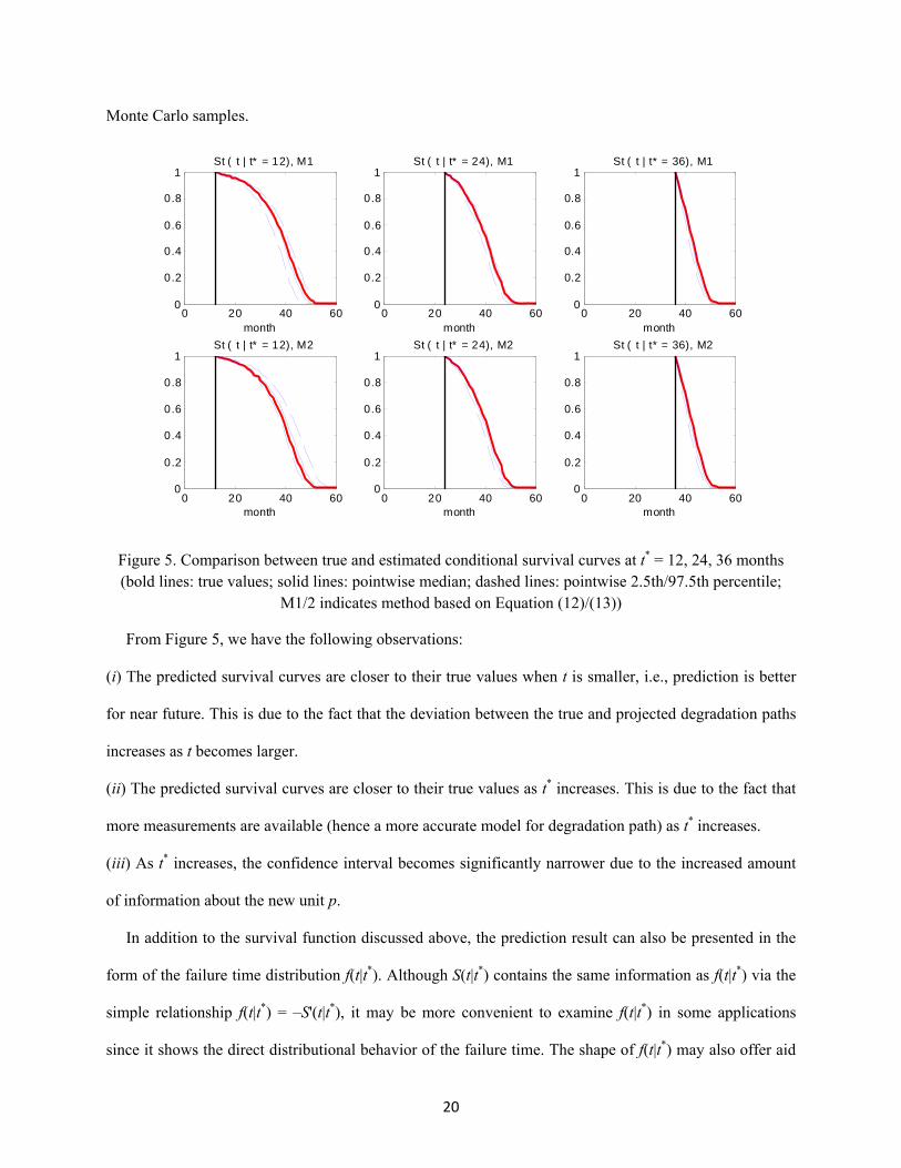
20  

Monte Carlo samples.

Figure 5. Comparison between true and estimated conditional survival curves at t* = 12, 24, 36 months (bold lines: true values; solid lines: pointwise median; dashed lines: pointwise 2.5th/97.5th percentile;

M1/2 indicates method based on Equation (12)/(13))

From Figure 5, we have the following observations:

(i) The predicted survival curves are closer to their true values when t is smaller, i.e., prediction is better

for near future. This is due to the fact that the deviation between the true and projected degradation paths

increases as t becomes larger.

(ii) The predicted survival curves are closer to their true values as t* increases. This is due to the fact that

more measurements are available (hence a more accurate model for degradation path) as t* increases.

(iii) As t* increases, the confidence interval becomes significantly narrower due to the increased amount

of information about the new unit p.

In addition to the survival function discussed above, the prediction result can also be presented in the

form of the failure time distribution f(t|t*). Although S(t|t*) contains the same information as f(t|t*) via the

simple relationship f(t|t*) = ‒S'(t|t*), it may be more convenient to examine f(t|t*) in some applications

since it shows the direct distributional behavior of the failure time. The shape of f(t|t*) may also offer aid

0 20 40 600

0.2

0.4

0.6

0.8

1

month

St ( t | t* = 12), M1

0 20 40 600

0.2

0.4

0.6

0.8

1

month

St ( t | t* = 12), M2

0 20 40 600

0.2

0.4

0.6

0.8

1

month

St ( t | t* = 24), M1

0 20 40 600

0.2

0.4

0.6

0.8

1

month

St ( t | t* = 24), M2

0 20 40 600

0.2

0.4

0.6

0.8

1

month

St ( t | t* = 36), M1

0 20 40 600

0.2

0.4

0.6

0.8

1

month

St ( t | t* = 36), M2

21  

to the decision making of maintenance strategies. The true and estimated survival functions from

Equation (12) and Equation (13) in Figure 5 are converted into f(t|t*) and shown in Figure 6. Note that the

pointwise intervals in Figure 5 are converted into mean curves.

t* = 12  t* = 24 t* = 36

Figure 6. Failure time distribution at different prediction time instants

3.2. Performance analysis

The simulation study conducted above is a demonstration based on a single unit with bp = [3.0, 0.015,

0.012]. To get a better idea of the overall performance of the proposed model, more analysis has been

conducted in this section.

First of all, we shall extend the simulation study to multiple units. Here, the same simulation setting

from the previous section with database sample size N = 1,000 is used. The prediction performance is

assessed through 3,000 in-service units with bp values randomly sampled from the population distribution

( , )b bN . For the performance metric, the mean absolute error (MAE) and the mean absolute

percentage error (MAPE) are used. The MAPE is a scale-independent percentage-based measure of

accuracy. Mathematical definitions for both metrics are given as

**

1 1

( )1 1( ) , 100 ,

J Jj j

j jj j j

mrl t TMAE mrl t T MAPE

J J T

10 20 30 40 50 60 70

0.00

0.0

10.

020.

030.

040

.05

0.06

Time

Pro

bab

ility

10 20 30 40 50 60 70

0.00

0.0

10.

020.

030.

040

.05

0.06

10 20 30 40 50 60 70

0.00

0.0

10.

020.

030.

040

.05

0.06

TrueM1M2

30 40 50 60 70

0.00

0.01

0.02

0.03

0.04

0.0

50

.06

0.0

7

Time

Pro

bab

ility

30 40 50 60 70

0.00

0.01

0.02

0.03

0.04

0.0

50

.06

0.0

7

30 40 50 60 70

0.00

0.01

0.02

0.03

0.04

0.0

50

.06

0.0

7

TrueM1M2

35 40 45 50 55 60 65 70

0.00

0.0

20

.04

0.06

0.08

Time

Pro

bab

ility

35 40 45 50 55 60 65 70

0.00

0.0

20

.04

0.06

0.08

35 40 45 50 55 60 65 70

0.00

0.0

20

.04

0.06

0.08

TrueM1M2

22  

where mrlj(t*) and Tj represent the mean RUL prediction at t* and its true value for the jth unit,

respectively. Table 2 summarizes the results, where the mean RUL predictions are based on Equation (12)

and the J has been set as 3,000.

Table 2. Prognostic performance summary for 3000 prediction trials

MAE MAPE t* = 0  12.0743 28.4864

t* = 12  1.9162 5.8417 t* = 24 1.0943 4.7657 t* = 36 0.9635 8.6903

According to the results given in Table 2, we can see that MAE consistently decreases as prediction

time increases, confirming that the prediction accuracy gets better at the later stage of the prediction. For

the scale-independent MAPE, although there is a small increment at the last stage of the prediction, the

general decreasing trend still holds. This further confirms our previous observations.

In real-world engineering applications, a historical database with N = 1,000 samples is rarely practical.

Here we demonstrate the model performance with smaller sample sizes. Table 3 presents the mean RUL

prediction results based on various historical sample sizes. Note that the results are computed by Equation

(12). The reduced sample size of the historical database does not cause notable problems for the

parameter estimation, only with increased standard error which is expected. This shows the proposed

method can be implemented with a small sample size, which may often be the case in practice.

Table 3. Mean RUL prediction from various sample sizes

True

values MRL estimates (N=1000) MRL estimates (N=50) MRL estimates (N=20)

Mean Std error Mean Std error Mean Std error t* = 0  37.376 28.465 1.318 29.949 4.983 33.921 9.447

t* = 12  26.274 24.862 1.538 25.344 3.864 26.944 6.253 t* = 24 15.138 14.822 0.417 15.147 1.909 16.377 4.507 t* = 36 6.837 6.131 0.391 6.375 1.762 7.252 3.274

4. Case study on battery data

In this section, we use real data from an automotive lead-acid battery aging test to demonstrate the

23  

proposed method. Because the aging process of automotive batteries is typically very slow and it takes

several years for a battery to fail, the data is obtained from an accelerated aging test based on the aging

cycle defined in SAE J2801 (SAE International (2013)). In this test, a battery is considered as dead when

it fails to crank the engine. The dataset contains 15 batteries with two different types: 8 batteries of type A

and 7 of type B. One battery of type A showed drastically different behavior from others and hence

removed from this study. The resistance evolution of the remaining 14 batteries is shown in Figure 7.

Note that resistance measurement is not necessarily available every week during the entire life of a battery.

Due to confidentiality, the data presented in Figure 7 has been slightly modified from the original data,

but this modification does not affect our study here. In the figure, the battery marked with stars is used for

prediction and not included in the database during model fitting.

Figure 7. Battery resistance data from an accelerated aging test

(stared line: the battery to be predicted)

To the best of the authors’ knowledge, there is no general physical form for the degradation path of

lead-acid battery resistance. Therefore, a quadratic degradation path in the random effects model is used.

Predictions are made for the battery at the t* = 5th and 10th week based on the resistance measurements up

to these time points. With 1000 random samples generated from the posterior distribution of bp, the

estimated survival curves are calculated based on Equation (8) and their point-wise quantiles shown in

Figure 8.

24  

Figure 8. Estimated survival functions at t* = 5 and 10

As expected, the point-wise interval gets narrower as more data have been collected. The estimated

mean RUL of the battery is 5.99 weeks at t* = 5 and 3.02 weeks at t* = 10 based on Equation (12); 6.63

weeks at t* = 5 and 2.90 weeks t* = 10 based on Equation (13). This again shows that the prediction

results are becoming more accurate at the later stage of prediction. Considering the fact that this battery

actually failed at the 13th week, the prediction results are quite good.

5. Conclusions

In this paper, a prognostic framework based on the joint modeling of time-to-event data and

degradation signal has been proposed for RUL prediction of individual units under hard failure. The

framework features a two-stage approach where modeling and parameter estimation are done offline

based on historical data of previously recorded units, and online real-time RUL prediction for new units

being used in the field. This two-stage approach allows the prediction to be made quickly with minimal

requirement on computation; hence it has the potential to be implemented on individual units in the field

where powerful computing platforms are not available (e.g., the prediction of a battery RUL on a vehicle

micro-controller). Two methods for estimating the conditional survival function have been proposed and

tested in a simulation study. The Equation (12) is accurate but relatively slow, while Equation (13) is a

conservative estimator but significantly faster. The choice of the two methods should be made depending

on the actual application: (13) is preferred for risk adverse users and/or when computational load is of

primary concern.

25  

In this paper, assessment of the algorithm’s prediction accuracy is rather subjective due to lack of

rigorous methods in the related literature. In engineering applications, a preferable method for assessing

predictive accuracy should be based on some commonly accepted criteria such as Type I and II error rates.

Also, this study focuses on the mean RUL point estimate. In practice, the interval estimate gives richer

information to the user than the point estimate. Since the RUL distribution is readily available from the

proposed joint prognostic framework, constructing the failure prediction interval could be an interesting

topic to investigate. These will be studied and reported in future.

Acknowledgements

This work is supported by the National Science Foundation CMMI Grant # 1335129 and the National

Natural Science Foundation of China Grant # 11301441. The authors wish to thank the Associate Editor

and three referees for their helpful comments that have led to improvements of this paper.

References

Bycott, P., and Taylor, J. (1998) A comparison of smoothing techniques for CD4 data measured with

error in a time-dependent Cox proportional hazards model. Statistics in Medicine, 17(18), 2061-2077.

Cox D.R. (1972) Regression models and life-tables. Journal of the Royal Statistical Society, Series B, 34,

187-220.

Cugnet, M., Sabatier, J., Laruelle, S., Grugeon, S., Sahut, B., Oustaloup, A., and Tarascon, J. (2010) On

lead-acid-battery resistance and cranking-capability estimation IEEE Transactions on Industrial

Electronics, 57(3), 909-917.

Elwany, A., and Gebraeel, N. (2009) Real-time estimation of mean remaining life using sensor-based

degradation models. Journal of Manufacturing Science and Engineering, 131(5), 051005-1-051005-9.

26  

Gebraeel, N. (2006) Sensory-updated remaining useful life distributions for components with exponential

degradation signals. IEEE Transactions on Automation Science and Engineering, 3(4), 382-393.

Gebraeel, N., Lawley, R., Li, R., and Ryan, J. (2005) Residual-life distributions from component

degradation signals: A Bayesian approach. IIE Transactions, 37(6), 543-557.

Gorjian, N., Ma, L, Mittinty, M., Yarlagadda, P., and Sun, Y. (2009) A review on degradation models in

reliability analysis. Proceedings of the 4th World Congress on Engineering Asset Management, Athens,

Greece, Sep. 2009.

Hsieh, F., Tseng, Y-K., and Wang, J-L. (2006) Joint modeling of survival and longitudinal data:

likelihood approach revisited. Biometrics, 62(4), 1037-1043.

Jardine, A., Lin, D., and Banjevic, D. (2006) A review on machinery diagnostics and prognostics

implementing condition-based maintenance. Mechanical Systems and Signal Processing, 20(7), 1483-

1510.

Jensen, J. L. W. V. (1906) Sur les fonctions convexes et les inégalités entre les valeurs moyennes Acta

Mathematica. 30(1), 175-193.

Laird, N. M., and Ware, J.H. (1982) Random effects model for longitudinal data. Biometrics, 38(4), 963-

973.

Liao, H., Zhao, W., and Guo, H. (2006) Predicting remaining useful life of an individual unit using

proportional hazards model and logistic regression model. Proceedings of the Annual Reliability and

Maintainability Symposium, Newport Beach, CA, 2006.

Lu, C., and Meeker, W. (1993) Using degradation measures to estimate a time-to-failure distribution.

Technometrics, 35(2), 161-174.

27  

Pauler, D. K., and Finkelstein, D.M. (2002) Predicting time to prostate cancer recurrence based on joint

models for non-linear longitudinal biomarkers and event time outcomes. Statistics in Medicine, 21(24),

3897-3911.

Prentice, R. L. (1982) Covariate measurement errors and the parameter estimation in a failure time

regression model. Biometrika, 69(2), 331-342.

Rizopoulos, D. (2011) Dynamic predictions and prospective accuracy in joint models for longitudinal and

time-to-event data. Biometrics, 67(3), 819-829.

Rizopoulos, D., and Verbeke, G. (2008) Shared parameter models under random effects misspecification.

Biometrika, 95(1), 63-74.

SAE International (2013) Comprehensive Life Test for 12 V Automotive Storage Batteries. SAE

Standards J2801.

Tsiatis, A., and Davidian, M. (2004) Joint modeling of longitudinal and time-to-event data: an overview.

Statistica Sinica, 14(3), 809-834.

Tsiatis, A., DeGruttola, V., and Wulfsohn, M.S. (1995) Modeling the Relationship of Survival to

Longitudinal Data Measured with Error. Applications to Survival and CD4 Counts in Patients with AIDS.

Journal of American Statistical Association, 90(429), 27-37.

Wang, P., and Coit, D. (2007) Reliability and degradation modeling with random or uncertain failure

threshold. Proceedings of the Annual Reliability and Maintainability Symposium, Las Vegas, NV, 2007.

Wang, Y., and Taylor, J. (2001) Jointly modeling longitudinal and event time data with application to

acquired immunodeficiency syndrome. Journal of American Statistical Association, 96(455), 895-905.

Wulfsohn, M., and Tsiatis, A. (1997) A joint model for survival and longitudinal data measured with error.

Biometrics, 53, 330-339.

28  

Ye, Z.S., and Chen, N. (2014) The inverse Gaussian process as a degradation model. Technometrics, to

appear.

Ye, Z.S., Shen, Y., and Xie, M. (2012) Degradation-based burn-in with preventive maintenance.

European Journal of Operational Research, 221 (2), 360-367.

Yu, I.T., and Fuh, C.D. (2010) Estimation of Time to Hard Failure Distributions Using a Three-Stage

Method. IEEE Transactions on Reliability, 59(2), 405-412.

Yu, M., Law, N., Taylor, J., and Sandler, H. (2004) Joint longitudinal-survival-cure models and their

application to prostate cancer. Statistica Sinica, 14(3), 835-862.

Yu, M., Taylor, J., and Sandler, H. (2008) Individual prediction in prostate cancer studies using a joint

longitudinal survival-cure model. Journal of American Statistical Association, 103(481), 178-187.

Zhang, X., Grube, R., Shin, K-K, Salman, M., and Conell, R. (2011) Parity-relation-based state-of-health

monitoring of lead acid batteries for automotive applications. Control Engineering Practice, 19(6), 555-

563.

Appendix

The likelihood function (7) can be rewritten in a matrix form as

* 2 /2 * * * * 2ˆ ˆ( | ) (2 ) exp ( ) ( ) / (2 )h m h T hp p p p p p p pp r b r Z b r Z b .

Based on prior distribution ˆˆ( ) ( , )p b bN b , the posterior distribution of bp , is

29  

* *

* * * * 12

* * * * * * * *2

1

( | ) ( | ) ( )

1 1 ˆˆ ˆexp ( ) ( ) exp ( ) ( )ˆ2 2

1exp ( ) ( ) ( ) ( )

ˆ2

1 ˆ exp2

h hp p p p p

h T h Tp p p p p p p b b p b

h T h T T h h T T Tp p p p p p p p p p p p

Tp b

p p

b r r b b

r Z b r Z b b b

r r b Z r r Z b b Z Z b

b

1 1 1

* * * * * *1 1 1

12 2 2

* *

2

ˆ ˆ ˆˆ ˆ ˆ ˆ

( ) ( ) ( )1 ˆ ˆ ˆˆ ˆexpˆ ˆ ˆ2

( )1 ˆexpˆ2

T T Tp b b p p b b b b b

T T h h Tp p p p p pT T T

p b p p b p b b p

Tp pT

C

b b b

Z Z Z r r Zb b b b

Z Zv

12b C

v

,(A1)

where C1 and C2 are constants not involving bp, and v is a k×1 vector defined as

1* * * *1 1

2 2

( ) ( )ˆ ˆ ˆˆ ˆ

T T hp p p p

p b b b

Z Z Z rv b .

Define

1* * * ** 1 1

2 2

1* ** 1

2

( ) ( )ˆ ˆˆ ˆˆ ˆ

( )ˆ ˆˆ

T T hp p p p

p b b b

Tp p

p b

Z Z Z r

Z Z

,

the result in (A1) can be rewritten as

1* * * *1 ˆˆ ˆ( | )

2

Thp p p p p p pp

b r b b

.

The above density defines a k-dimensional multivariate normal distribution * *ˆˆ( , )p pN .