Flight dynamics and simulation of a generic aircraft for

aeroservoelastic design

Pedro Tomas Marques Martins Margaridopedro.tomas.margarido@tecnico.ulisboa.pt

Instituto Superior Tecnico, Lisboa, Portugal

November 2016

Abstract

The emerging market of the aviation sector begins to request the need for tools to study the aeroser-voelastic behaviour of an aircraft. There are mathematical models for this kind of study, but itsinterpretation is not easy and many of them use the frequency domain.

In this thesis the aeroservoelastic equations of motion of a general aircraft for equilibrium conditionsin time domain were developed. A program was also developed, produced in C++R©, which integratesthese same equations, and that in the future may be included in other projects as an interconnection toolbetween different fields of aeronautics, such as aerodynamics, structural dynamics and flight control. Todevelop this tool, various integration methods were inspected and consequently the utility of each onewas found. Aeroelasticity consequences were also discussed and used to introduce the optimal control.

It was also carried out a flight simulator in MATLABR© using optimal control. The optimal controlbehaviour, more specifically the linear quadratic regulator, in the flight dynamics was also studied. Thisflight simulator allows the simulation of the motion for a general aircraft, adopting a set of aerodynamicsderivatives of general aircraft from the literature, on turbulent air flows and in engine failure cases inaircraft up to five engines. The simulation study in this thesis had more in mind to ensure that theaircraft maintains its equilibrium and course in critical situations, as referred above.Keywords: flight dynamics, optimal control, aeroservoelasticity, flight simulation, integration

1. IntroductionWith the increasing growth of high-performanceand cheap aircraft, the need for more realistic flightsimulators also grows. One of the crucial aspectson making the flight simulator more realistic is theconsideration of aircraft’s elastic properties (aeroe-lasticity).

Figure 1: Aeroelasticity (adapted from [4])

As seen in Figure 1, aeroelasticity has been de-fined as a science which studies mutual interactionsbetween aerodynamic forces and elastic forces, andthe influence of these interactions on airplane de-

sign. Some of the most rough phenomena on air-craft’s structure happen because of the aircraft’selastic properties. These physical phenomena, asthey will be described later, can be, for example,flutter, control reversal and others.[3]. That is whyaeroservoelasticity plays an important role on con-trolling and preventing these harmful effects fromhappening.

The goal of the dynamics integration tool is toguarantee future integration with aerodynamics,structures and flight control programs to simulatea generic aircraft dynamics during a time interval(∆t). The grey highlighted boxes in Figure 2 are themodules done and described throughout this thesis.

2. Theoretical Background

Several key disciplines such as flight simulators,aeroelasticity, aeroservoelasticity and mathematicalmethods used to simulate unsteady aerodynamicsand structural dynamics are briefly covered in thissection.

1

Figure 2: Interactions between modules

2.1. Flight SimulatorsFlight simulation is basically a way to recreate theconditions of a real flight. Several aeronautical ar-eas such as flight dynamics, navigation and aeroe-lasticity behavior can be studied in an artificialcomputational environment. As seen in Figure 3,

Figure 3: General structure from a flight simulator

a flight simulator is composed by several modules.The crucial module of a simulator is the dynamicsmodule and in a general way, all the other modulesare inputs or outputs of this major module. Thisdissertation has the objective of creating this signif-icant module, containing the structural dynamics ofthe aircraft. Then it may be used, when paired witha flight controller, to control the harmful aeroelasticeffects that may occur (aeroservoelasticity).

2.2. AeroelasticityStability and control; structural dynamics andstatic aeroelasticity - each one of these major dis-ciplines are a product from two of three types offorce. When all the three types of force are in-teracting, dynamic aeroelastic phenomena occur.Harmful aeroelastic phenomena grow when struc-ture deformation causes additional aerodynamicforces. Eventually, these additional forces may pro-duce more structural deformation, resulting in evengreater aerodynamic forces. These adverse phe-

nomena usually occur when there is an interactionbetween the three forces (dynamic aeroelastic phe-nomena), and an interaction between aerodynamicand elastic forces (static aeroelastic) [3]. Some ofthe most catastrophic phenomena are:

• Flutter: Flutter is an aeroelastic self-excitedunstable vibration in which the airstream en-ergy is absorbed by the lifting surface. The mo-tion involves both bending and torsional com-ponents which are basically simple harmonicoscillations with an unique flutter frequency;

• Divergence: A static instability of a liftingsurface of an aircraft in flight, at a speed calledthe divergence speed, where the elasticity ofthe lifting surface plays an essential role in theinstability.

2.3. AeroservoelasticityAeroservoelasticity (ASE) is the discipline of theaeronautical science that deals with the interactionof aircraft structural, aerodynamic, and control sys-tems. Though there were early sucesses in creatingactive flutter suppression systems and load allevia-tion systems, ASE still remains a vast experimentalarea and has still not reached operational status onany aircraft [9]. A possible block diagram for theaeroservoelasticy is seen in Figure 4.

Figure 4: General aeroservoelastic block diagram(adapted from [9])

Deformation happens or is usually increasedwhen there are gusts (disturbance input) or controlsurface deflection, as seen in the aeroelasticity plantfrom Figure 4. Deformation induces changes onthe aerodynamic forces acting on the aircraft, hencethe aerodynamic feedback loop. Therefore this cy-cle needs to be controlled, or in extreme cases, itmay lead to one of many catastrophic phenomenaas explained in the Section 2.2. Knowing these de-formation rates and the aeroelastic phenomena, itis possible to generate a control model to preventthese phenomena from happening. The flutter dy-namic pressure (pdF ) has an associated speed called

2

flutter velocity

pdF =1

2ρVFlutter . (1)

The goal of an aeroservoelastic model, is to closethe loop in order to increase the open-loop fluttervelocity [9].

3. Dynamics ModelIn this Section the equations of motion (EOM) of ageneric elastic aircraft will be defined.

3.1. Reference Frames and AnglesWhen working with a flight dynamics’ problem itis crucial to choose a proper reference frame thatspecifies the needs of the problem.

Figure 5: Fixed reference frame, FE , and aircraftreference frame, FB [8]

Before advancing to the definition of the equa-tions of motion, two reference frames, as seen inthe Figure 5, need to be chosen. The local NED(North-East-Down) coordinate system was chosenfor fixed frame (FE) and the RPY (Roll-Pitch-Yaw)was picked for the body axis system (FB). ThroughEuler angles (φ,ψ,θ) the transformation from theNED frame to the RPY frame is intuitive [8].

3.2. Rigid Body Flight DynamicsThe equations of motion are a result from the ap-plication of Newton-Euler formulation in classic me-chanics to the flight vehicle, in the fixed referenceframe (subscript E). Applying these, and con-sidering for now constant mass and constant iner-tia throughout time, two crucial equations emerge.One for linear moment

F =d

dt[mvE ] , (2)

where F represents the resultant of all externalforces applied on the aircraft, m is the aircraft’smass, vE the vehicle linear motion vector relativeto the fixed reference frame.

And finally the angular moment equation

M =d

dt[H]E =

d

dt[Iw]E =

d

dtIwE , (3)

where M represents the resultant external moment,H is the total moment relative to the aircraft’s cen-ter of mass. H is equal to the product of w, theangular velocity vector, with I being the inertia ten-sor matrix. The small disturbance theory when, ap-plied to the rigid body flight dynamics in a steadystate, as rectilinear flight, is a powerful tool that de-couples the motion into variables responsible for thelongitudinal and lateral motion. Considering singleengine contribution for forces and moments, (2) and(3) expand into two decoupled set of equations, onefor longitudinal motion

u = Xuu− w0q +Xww − gcos(θ0)θ +XδEδE+∑Nengi=1 XδT iδT i

w = Zuu+ u0q + Zww − gsin(θ0)θ + ZδEδE+∑Nengi=1 ZδT iδT i

q = Muu+ Mww + Mqq + Mθθ + MδEδE+∑Nengi=1 δT i(ziXδT i − xiZδT i)

θ = q

,

(4)and other for lateral motion

β = Yββ + p(Ypu0

+ α0) + r(Yru0− 1) + gcos(θ0)

u0φ

+YδAu0δA +

YδRu0δR

p = L′ββ + L′pp+ L′rr + L′δAδA + L′δRδR−∑Nengi=1 yiZδT iδT i

r = N ′ββ +N ′pp+N ′rr +N ′δAδA +N ′δRδR

+∑Nengi=1 yiXδT iδT i

φ = p+ tan(θ0)r

ψ = rcos(θ0)

,

(5)where Xi, Yi and Zi represent ith state variable in-duced force on the x, y and z axis respectively. TheLi, Mi and Ni represent ith state variable inducedmoment on the x, y and z axis, respectively.

3.3. Elastic Aircraft ConsiderationWhen aeroelastic effects are taken into account, newstate variables and their respective equations, repre-senting a set of generalized coordinates associatedwith the bending modes need to be added to theflight dynamics equations system, (4) and (5). Thevibration (bending, torsion, mixed, among others)modes can be represented using generalized coordi-nates

c1iqi + c2iqi + c3iqi = Fi (6)

where Fi is a generalized force, c1i, c2i and c3i arecoefficients of the ith generalized coordinate (qi)and of its rates. [5] Although it is possible to rep-resent the vibration mode by two first order, linear,differential equations

x1 = qi , x2 = qi , (7)

3

where

x1 = x2

x2 =−c2ic1i

x2 −c3ic1ix1 +

1

c1iFi . (8)

This pair of first order differential equations repre-senting the vibration mode can be used to augmentthe rigid body dynamics. Usually, the conventionfor enumerating vibration modes, is such that mode1 corresponds to the mode with lowest vibrationfrequency. So as the mode number increases, itsassociated frequency increases.

Assuming the conditions of the flight dynamicssystem (4) and (5) and the state vectors for longi-tudinal and lateral motions represented in equations(9) and (10)

xlong =[u w q θ λ1 σ1 ... λn σn

]T, (9)

xlat =[β p r φ ψ τ1 χ1 ... τn χn

]T,

(10)the flexibility effects of a general aircraft, for n vi-bration modes, can be represented as

u = Xuu− w0q +Xww − gcos(θ0)θ +XδEδE+∑Nengi=1 XδT iδT i +Xλ1

λ1 +Xσ1σ1 + ...+

Xλnλn +Xσnσnw = Zuu+ u0q + Zww − gsin(θ0)θ + ZδEδE+∑Neng

i=1 ZδT iδT i + Zλ1λ1 + Zσ1σ1 + ...+Zλnλn + Zσnσn

q = Muu+ Mww + Mqq + Mθθ + MδEδE+∑Nengi=1 δT i(ziXδT i − xiZδT i) +Mλ1λ1+

Mσ1σ1 + ...+Mλnλn +Mσnσn

θ = q

λ1 = σ1σ1 = −(2ξ1ω1 + η1σ1 )σ1 + (−ω1

2 + η1λ1 )λ1+η1uu+ η1ww + η1qq + η1δE δE+∑Nengi=1 η1δT i δT i + ...+ η1σnσn + η1λnλn

...

λn = σnσn = −(2ξnωn + ηnσn )σn + (−ωn2 + ηnλn )λn

+ηnuu+ ηnww + ηnqq + ηnδE δE+∑Nengi=1 ηnδT i δT i + ηnσ1σ1 + ηnλ1λ1 + ...+

ηnσn−1σn−1 + ηnλn−1

λn−1

,

(11)

β = Yββ + p(Ypu0

+ α0) + r(Yru0− 1) + gcos(θ0)

u0φ

+YδAu0δA +

YδRu0δR + Yτ1τ1 + Yχ1

χ1 + ...+

Yτnτn + Yχnχnp = L′ββ + L′pp+ L′rr + L′δAδA + L′δRδR−∑Neng

i=1 yiZδT iδT i + Lτ1τ1 + Lχ1χ1 + ...+

Lτnτn + Lχnχnr = N ′ββ +N ′pp+N ′rr +N ′δAδA +N ′δRδR+∑Neng

i=1 yiXδT iδT i +Nτ1τ1 +Nχ1χ1 + ...+Nτnτn +Nχnχn

φ = p+ tan(θ0)r

ψ = rcos(θ0)

τ1 = χ1

χ1 = −2ξAωAχ1 +−ωA2τ1 + µ1ββ + µ1pp+µ1rr + µ1δA

δA + µ1δRδR + ...+ µ1χn

χn+µ1τn

τn...τn = χnχn = −2ξZωZχn +−ωZ2τn + µnββ + µnpp+

µnrr + µnδA δA + µnδR δR + µnχ1χ1 + µnτ1 τ1

+...+ µnχn−1χn−1 + µnτn−1

τn−1

,

(12)where λ and τ represent the displacement of sym-metrical and asymmetrical bending mode, µnτ andηnλ correspond to the structural derivatives withrespect to the nλ and nτ bending modes. Vari-ables χ and σ are used to facilitate interpretationand maintain the system as a first order differentialequations system. The variables ξ and ω correlateto the damping ratio and natural frequency.

4. Dynamics Model ImplementationOne of the goals of this thesis, besides the flightcontroller, is the implementation of a standaloneaircraft dynamics client. The dynamics equationsfor this C++ R© program were equations (11) and(12).

The center piece of this developed program isits integration function. This integration functioncomes from the Boost c© C++ R© library, an open-source extensive used library that provides a widerange of platform agnostic functionality that STL(Standard Template Library) missed [1].

The integration function was integrate adaptive.It performs the time evolution, for each time stepdt, of the ordinary differential system from somestarting time t0 to a given end time t1, a startingstate x0 and the stepper, that is nothing more thanthe mathematical method used during the integra-tion. This function also has the benefit of callingthe observer at equidistant times separated by dt.

4.1. Inputs and OutputsThis client will receive information from severalmodules such as: aerodynamics, structural dynam-ics, flight controller and propulsion model. Then,it will be possible to simulate the dynamics dur-ing a time interval (∆t). The objective is to sup-ply the other modules with the aircraft’s trajec-tory (xE ,yE ,zE), velocities (uB ,vB ,wB), accelera-

4

tions (axB ,ayB ,azB ), euler angles (φ,ψ,θ) and angu-lar rates (p,q,r) during that time interval.

4.2. Type of SteppersThe stepper is the mathematical model used duringthe step integration. There are plenty of steppersand each one has its purpose and use. For this typeof ODE problem there are three kinds of steppers:

• Basic steppers: As the name enunciates,these are the normal steppers. Some of themare euler and runge kutta cash karp54;

• Error steppers: Steppers that provide an er-ror estimation. Besides also being a basic step-per, runge kutta cash karp54 provides also anerror estimation;

• Controlled steppers: Built on error step-pers, this kind of stepper may decide to mod-ify the integration time step if an error criteriafinds the suggested time step inadequate. Thecontrolled runge kutta will be the consideredcontrolled stepper.

4.3. Stepper ComparisonFor the stepper comparison test, the trim conditionstability derivatives data from the three enginedDassault Falcon 7X, was used. The standard inte-gration solver used in SIMULINK R©, the Dormand-Price, which is a controlled stepper, will be used asa reference.

Figure 6: Dynamic response of the Dassault Falcon7X (v,p,w,q)

In Figure 6, it is exposed the integration resultsof the Dassault Falcon 7X in a certain flight condi-tion ( Dassault Falcon 7X δA = 5◦, δR = 0◦, δE =

5◦, no engine throttle and null initial state condi-tions). The time of the integration is ten secondsand the time step (dt) for Euler and Runge-Kuttais 0.2 seconds. The plan is to spot the differencesbetween integration steppers and eventually chooseone for the dynamics integration problem.

The Euler method possesses significant accuracyproblems as it only corresponds to the two firstterms in the Taylor series, these accuracy problemsare visible in the w plot. As its error propagationgrows with the number of time steps and their size,it can become divergent in some cases as in the vplot.

The 4th order Runge-Kutta integration schemeshows suitable results for the dynamics of this flightcondition. Although if the system has certain initialcondition or states for the control variables, it canovershoot.

The controlled Kutta stepper internally varies thetime step size. However, it has a considerable set-back which is that the user has no power in thechoice of the controlled stepper time step. As thedynamics integrator goal is to interconnect to othersoftware infrastructures, it needs to have a well de-fined time step in order to synchronize correctly.

In the light of these results, the dynamics inte-grator default stepper is the Runge-Kutta stepperof 4th order. Nevertheless with the usage of theintegrate adaptive function, the option of using acontrolled stepper or another basic stepper is opento the user. The need for controlled stepper mightappear, especially, for aircraft that have overshoot-ing responses.

5. Flight ControlIn this Section the requirements for flight controland the final model state forms will be presented.

5.1. Simulation DomainThe flight controller of this project will be repre-sented in state-space form,{

x = Ax + Buy = Cx + Du

. (13)

The first equation in (13) is the state equation. Thisequation is a first order, vector differential equation,where the x represents the state vector, u the con-trol vector, A the state coefficient matrix and Bthe driving matrix. The second equation in (13) isthe output equation, which is merely an algebraicequation that solely depends upon the state vector.Where y is the output vector, and the matrices Cand D the output and direct matrix respectively [5].The stability of the system is verified by looking atthe eigenvalues of the state coefficient matrix A. Ifthese eigenvalues have negative real part, then it issafe to say that the system, x = Ax(t) is asymp-totically stable.

5

5.2. Longitudinal ControlFor the lateral mode the control will be done in theflight path angle (γ) and longitudinal speed (u).The flight path angle (γ) needs to be added as astate, and keeping in mind that the vertical velocity(w) can be approximated, for small perturbations,as a function of the angle of attack (α)

γ = θ − α→ θ = γ +w

u0. (14)

When transforming the system (4) into state-spaceand substituting , the pitch angle (θ) for flight path(γ), the longitudinal state-space emerges

xLongγ = ALongγxLongγ + BLongγuLong =Xu Xw − gcos(θ0)

u0−w0 −gcos(θ0)

Zu Zw − gsin(θ0)u0

u0 −gsin(θ0)

Mu Mw + Mθ

u0Mq Mθ

−Zuu0−Zwu0

+ gsin(θ0)u20

0 gsin(θ0)u0

uwqγ

+XδE XδT 1

... XδTNeng

ZδE ZδT 1... ZδTNeng

MδE (ziXδT 1− xiZδT 1

) ... (zNengXδTNeng− xNengZδTNeng )

−ZδEu0

−ZδT 1

u0...

−ZδT Nengu0

uLong ,

(15)

where

uLong =[δE δT 1 ... δTNeng

]T. (16)

Two additional states (xu and xγ) were added toprevent static error on the longitudinal controllablestates, consequently increasing the size of system’s(15) A, B and x.

5.3. Lateral ControlOnly one variable will be controlled in the lateralmode, the heading angle (λ). It can be defined asthe sum of slide slip angle (β), with the yaw angle(ψ)

λ = β + ψ . (17)

This will be the fifth lateral state substituting theyaw angle (ψ). The lateral equations (5) are thentransformed into the state-space

xLatλ = ALatλxLatλ + BLatλuLat =Yβ

Ypu0

+ α0Yru0− 1 gcos(θ0)

u00

L′v L′p L′r 0 0N ′v N ′p N ′r 0 00 1 tan(θ0) 0 0

YβYpu0

+ α01

cos(θ0)+ Yr

u0− 1 gcos(θ0)

u00

βprφλ

+

YδAu0

0 ... 0YδRu0

L′δA −y1ZδT 1... −yNengZδTNeng L′δR

N ′δA y1XδT 1... yNengXδTNeng

N ′δR0 0 ... 0 0YδAu0

0 ... 0YδRu0

uLat . (18)

where

uLat =[δA δT 1 ... δTNeng δR

]T. (19)

An additional state (xλ) was added to prevent staticerror on the heading angle (λ), consequently in-creasing the size of system’s (18) A, B and x.

5.4. Flying and Handling QualitiesAircraft flying qualities are defined by a number ofparameters in the complex frequency domain. Inequation (20) there are two of these important pa-rameters, damping ratio (ξ) and undamped naturalfrequency (ωn).

ωn = |κ|ξ = −cos(∠κ)

(20)

In this dissertation project it is needed to ensurethat for a certain mission, the aircraft has the bestflying qualities. The specification used is the MIL-F-8785, Military Specification - Flying Qualities ofPiloted Airplanes published in 1980. The level offlying qualities on this specification depends uponthe aircraft class and flight phase [6].

5.5. Disturbances State-space FormTo include the disturbances, a new matrix is addedinto the aircraft dynamics state-space form (13)

x = Ax + Bu + Ed , (21)

where d represents the disturbance states

dcoupled =[dLong dLat

]T(22)

=[ug wg qg vg pg rg

]T. (23)

and E the associated disturbance influence matrix.

5.6. SIMULINK R© State-Space modelThe common state-space SIMULINK R© model couldnot be used for this project because it does not in-clude the associated disturbance influence matrix,E. The model in Figure 7, satisfies the state-spaceequation (21) where the A and the B matrices are

Figure 7: State-Space model implemented inSIMULINK R©

formed by the matrices of equations (15) and (18).

6. Optimal ControlThe goal is to examine the optimal control tech-nique used for the flight controller. An example offlutter suppression on a two-dimensional aeroelasticairfoil will be used to demonstrate the utility of thelinear quadratic regulator.

6

6.1. Aeroservoelastic Optimal Control

To introduce the linear quadratic regulator (LQR),a flutter suppression controller of a two-dimensionalaeroelastic airfoil represented in Figure 8, will bedemonstrated.

Figure 8: The 2-D cross-section of an airfoil [7]

This is a typical aeroservoelastic problem, whenthe airspeed increases the elastic airfoil starts de-flecting and therefore increasing the aerodynamicforces acting on it, leading to bigger deflections and,as a result, bigger oscillations. There is an airspeedlimit, called flutter velocity, for marginally stableoscillations. The results of [7] were reproduced us-ing MATLAB R© and SIMULINK R©.

6.2. Open Loop Aeroservoelastic Problem

In this example the flutter velocity (VFlutter) forthis airfoil is 297.4 m/s. In order to begin the sim-ulation, it is considered that there is an initial con-dition for the state variables (x0).

0 0.5 1 1.5 2 2.5-0.1

0

0.1

Rad

ians

(ra

ds)

Pitch angle α V=Vflutter

Open-loop

0 0.5 1 1.5 2 2.5

Time (s)

-0.05

0

0.05

Rad

ians

(ra

ds)

Flap angle β V=Vflutter

Open-loop

Figure 9: Pitch and flap angle variation over timeconsidering flutter velocity (V = Vflutter = 297.4m/s) on open-loop

As seen in Figure 9, if the airspeed is exactlythe flutter velocity (V = VFlutter = 297.4 m/s),the system remains marginally stable throughoutall simulation. Marginally stable means that thematrix A has at least one eigenvalue with zero realpart. The objective is now to implement a controllaw to suppress flutter.

6.3. Linear Quadratic RegulatorThere are two great advantages when solving a lin-ear quadratic problem. Firstly, the control is a fullstate linear feedback law

u = −Kx , (24)

and secondly, this resulting feedback control lawwill ensure that the system in closed-loop is stableand robust, but only if the system is controllableand stabilizable [5]. This method is based in theoptimization and minimization of the system’s per-formance index J

J =1

2

∫ ∞0

(xTQx + εuTRu)dt . (25)

Equation (25) represents a trade-off between, x, uand two matrices Q and R. The state vector xbehaves as a constrain to the minimization of theperformance index, J. The ε is a parameter thatdetermines the relative weights.

6.4. Closed Loop Aeroservoelastic ProblemIn this particular aeroservoelastic case, LQR wasapplied as a control method in the pursuance offinding a control function u(t) to stabilize the sys-tem. This control function will have the form pre-sented in equation (24)

u(t) = −KLQRx(t) , (26)

and the closed loop system

x(t) = Ax(t) + Bu(t) →x(t) = (A−BKLQR)x(t) →

x(t) = A∗x(t) ,

(27)

where A∗ is the the augmented plant matrix.Matrices Q and R are square and symmetric ma-

trices and they can be time-dependent. The stateweighting matrix Q, is a positive definite matrixand the control cost matrix, R is a positive semi-definite matrix. The objective of these matrices isto regulate the importance of states and inputs vari-ables in the considered problem.

After choosing the Q and R and considering theflutter velocity (Vflutter) as 297.4 m/s, the closedloop dynamic response is given in Figure 10.

0 0.5 1 1.5 2 2.5-0.1

-0.05

0

0.05

0.1

Rad

ians

(ra

ds)

Pitch angle α V=Vflutter

Closed-loop LQR

0 0.5 1 1.5 2 2.5

Time (s)

-0.05

0

0.05

Rad

ians

(ra

ds)

Flap angle β V=Vflutter

Closed-loop LQR

Figure 10: Pitch and flap angle variation over timeconsidering flutter velocity (V = Vflutter = 297.4m/s) on closed-loop

7

Closing the loop stabilized the system. This sys-tem that once was marginally stable on the open-loop, now is completely stable having it’s oscilla-tions ending after about one and a half seconds.The full state feedback gain made the zero real parteigenvalues of open-loop translate to real negativepart eigenvalues in the closed loop.

6.5. Bryson’s MethodSince the definition of matrices Q and R can be ar-bitrary, there is a method called Bryson’s methodin which it suggests that each term of the diago-nal matrices, Q and R, is the inverse square of themaximum value expected for the variable on thesimulation time. As it follows

Q = diag(Qi)⇒ Qi =1

x2imax, R = diag(Ri)⇒ Ri =

1

u2imax.

(28)In the flight control system, u2imax and x2imax are thevalues indicating the extreme of the perturbationswanted for ui or xi for the closed loop during amaneuver. This method is a good starting point todefine these matrices and will be used in the flightcontrol problem. [2]

6.6. Schematic of the Flight Controller ModelThe desired control states are longitudinal speed,flight path angle and heading angle. The flight con-troller or the pilot inserts references for these statesand the model follows them, aided by the linearquadratic regulator feedback gains. Controllablestates feedback will then be

u = −[Ku Kγ Kλ

] u− urefγ − γrefλ− λref

−KLQRother

wqβprφ

(29)

6.7. SIMULINK R© Flight Controller ModelThe SIMULINK R© flight controller model is in Fig-ure 11. It gathers the concepts developed in previ-ous sections, to create a ready-to-use SIMULINK R©

flight controller model.

Figure 11: Flight controller model created inSIMULINK R©

The dynamics block, named as Space-State Sys-tem, is defined in Figure 7 and it includes a turbu-lence model. This turbulence model can be toggledoff by simply unchecking the ’Turbulence on’ box,and thus having a non-turbulent simulation. Thecontrol part of the model was built based in equa-tion (29). It is assumed a flight with no side slip,hence the reference for β being zero.

6.8. Linear Quadratic Regulator Script

The first step of the flight controller is to assure theaircraft dynamic modes have level 1 flying qualities.In order to reach that goal, several scripts and func-tions were created in MATLAB R© applying the con-cepts explained. The objective is to use the linearquadratic regulator as a stability augmentation sys-tem. However, as this flight controller is designedfor a general aircraft, Bryson’s method was imple-mented for an appropriate pole placement.

7. Flight Simulation

Initially, open-loop dynamics of the flight conditionsfor the Airbus A400M are analysed. Then, the goalis to use the flight controller to follow a reference inthe case of engine failure.

7.1. Open-Loop Dynamics

The aircraft used for the engine failure test is thefour engine Airbus A400M. From observing Table

Airbus A400M

Longitudinalmotion

Phugoidκphu1

= -0.066 +0.0883iκphu2

= -0.066 - 0.0883i

Short periodκsp1= -7.47 + 3.23iκsp1 = -7.47 - 3.23i

Lateralmotion

Spiral κspi = 0.0840Roll κroll = -1.26

Dutch Rollκdr1 = -0.141 + 1.82iκdr2 = -0.141 - 1.82i

Heading mode κλ = 0

Table 1: Open-loop dynamic modes eigenvalues

7.1, it is possible to conclude that the phugoid haslevel three and the short period has level two. Inthe lateral motion, the spiral mode is stable andthus level one, roll is also level one and dutch roll iscategorized as level two. Overall, the longitudinaland lateral motions of the aircraft do not have thelevel one flying qualities requirement. The LQRscript must place the poles of these dynamic modes,in such a way that the level one flying qualities ofthe aircraft are satisfied.

7.2. Engine Failure

In this section, it is assumed that the left enginesof the four engine Airbus A400M (δT1 and δT2) aremalfunctioning and therefore providing no thrust tothe aircraft

δT1 = 0 , δT2 = 0 . (30)

8

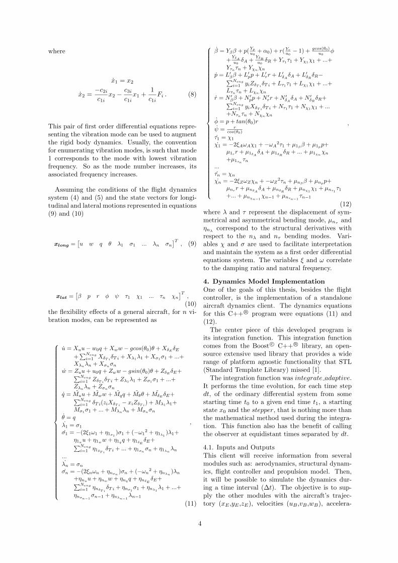
The control surfaces available for the aircraft arethen δT3

, δT4, δE , δA and δR. The goal is to perform

a climb (γref = 1◦) while maintaining heading (λref= 0◦). The reference for longitudinal velocity ismaintained at the trim velocity (uref = u0).

The script is then called and proceeds to find levelone flying qualities for a control penalty parame-ter of ε = 10. Table 7.2 contains the closed loopeigenvalues for ε = 10 and also for two additional εvalues.

Control penalty parameter (ε) 10 40 80

Longitudinalmotion

Phugoid(κphu1,2

)-0.597 ± 0.252i -0.414 ± 0.36i -0.369 ± 0.36i

Short period(κsp1,2)

-11.3 ± 4.37i -6.86 ± 5.23i -5.39 ± 4.92i

Lateralmotion

Spiral(κspi)

-0.631 -0.603 -0.569

Roll(κroll)

-3.36 -2.54 -2.28

Dutch roll(κdr1,2)

-1.98 ± 2.65i -1.33 ± 2.41i -1.08 ± 2.26i

Table 2: Closed loop poles for ε = 10, ε = 40 and ε= 80

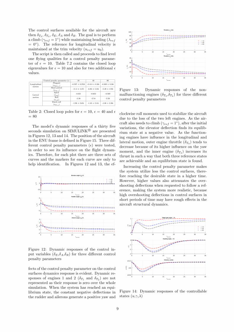
The model’s dynamic responses of a thirty fiveseconds simulation on SIMULINK R© are presentedin Figures 12, 13 and 14. The position of the aircraftin the ENU frame is defined in Figure 15. Three dif-ferent control penalty parameters (ε) were tested,in order to see its influence on the flight dynam-ics. Therefore, for each plot there are three sets ofcurves and the markers for each curve are only tohelp identification. In Figures 12 and 13, the ef-

0 5 10 15 20 25 30 35tseconds

-10

0

10

δE (

º)

Elevator angle ( δE) (º)

ǫ = 10ǫ = 40ǫ = 80

0 5 10 15 20 25 30 35tseconds

-5

0

5

δR

(º)

Rudder angle ( δR

) (º)

0 5 10 15 20 25 30 35tseconds

-4

-2

0

2

4

δA (

º)

Aileron angle ( δA

) (º)

Figure 12: Dynamic responses of the control in-put variables (δE ,δA,δR) for three different controlpenalty parameters

fects of the control penalty parameter on the controlsurfaces dynamics response is evident. Dynamic re-sponses of engines 1 and 2 (δT1

and δT2) are not

represented as their response is zero over the wholesimulation. When the system has reached an equi-librium state, the constant negative deflections inthe rudder and ailerons generate a positive yaw and

0 5 10 15 20 25 30 35tseconds

0

20

40

60

80

100

δT

3

(%

)

Throttle (δT

3

) (%)

ǫ = 10ǫ = 40ǫ = 80

0 5 10 15 20 25 30 35tseconds

0

10

20

30

40

δT

4

(%

)

Throttle (δT

4

) (%)

Figure 13: Dynamic responses of the non-malfunctioning engines (δT3 ,δT4) for three differentcontrol penalty parameters

clockwise roll moments used to stabilize the aircraftdue to the loss of the two left engines. As the air-craft also needs to climb (γref = 1◦), after the initialvariations, the elevator deflection finds its equilib-rium state at a negative value. As the function-ing engines have influence in the longitudinal andlateral motion, outer engine throttle (δT4

) tends todecrease because of its higher influence on the yawmoment, and the inner engine (δT3) increases itsthrust in such a way that both three reference statesare achievable and an equilibrium state is found.

Increasing the control penalty parameter makesthe system utilize less the control surfaces, there-fore reaching the desirable state in a higher time.However, higher values also attenuates the over-shooting deflections when requested to follow a ref-erence, making the system more realistic, becausehigh overshooting deflections in control surfaces inshort periods of time may have rough effects in theaircraft structural dynamics.

0 5 10 15 20 25 30 35tseconds

0

0.5

1

γ (

º)

Flight path angle, γ (º)

ǫ = 10ǫ = 40ǫ = 80

0 5 10 15 20 25 30 35tseconds

-3

-2

-1

0

λ (

º)

Heading angle, λ (º)

0 5 10 15 20 25 30 35tseconds

140.8

141

141.2

u (m

/s)

Velocity u (m/s)

Figure 14: Dynamic responses of the controllablestates (u,γ,λ)

9

In Figure 14, the desirable states dynamic re-sponses are represented. These dynamic responsesare the consequence of the control surfaces deflec-tions seen in Figures 12 and 13. When the systemallows for higher control deflections (ε = 10), thereference state is reached faster than when the con-trol action is more limited (ε = 80). However, forreasonable values of ε and assuming the system isstable, this final reference state is always reached asseen in Figure 14.

0 500 1000 1500 2000 2500 3000 3500 4000 4500 5000y

ENU (m)

-80

-60

-40

-20

0

x EN

U (

m)

XY Plane

ǫ = 10ǫ = 40ǫ = 80

0 500 1000 1500 2000 2500 3000 3500 4000 4500 5000y

ENU (m)

1000

1020

1040

1060

1080

1100

z EN

U

YZ Plane

Figure 15: Flight trajectory seen in XYENU andY ZENU planes (γref = 1◦, λref = 0◦ and uref =u0)

The representation of the states transformed intopositions on the XYENU and Y ZENU planes areshown in 15. The aircraft’s trajectory is repre-sented in the ENU reference frame, to facilitate vi-sual interpretation of the results. Initially the lackof thrust in the left engines make the aircraft de-viate to the left (negative YENU ) but eventuallythrough the control surfaces deflections the head-ing is stabilized.

8. ConclusionsThis dissertation not only developed a crucial piecefor a future aeroservoelastic tool but also a flightcontroller that can possibly be embedded into it.

The integrator results depend highly on the step-per used. For aircraft with low and medium ma-noeuvrability, an error stepper is recommended,although for high manoeuvrability aircraft a con-trolled stepper is the one to use as a result of over-shooting responses and high variations in short pe-riods of time.

The defined trim condition aeroservoelasticmathematical equations of motion are also left ina general state, as it is difficult to define the num-ber of bending modes required. This number ofvibration modes rely upon not only on the approxi-mation needed to define the structural influence onflight dynamics, but also on the aircraft to be stud-ied.

The flight controller and mathematical model re-

sults were as expected, obtaining realistic resultson its simulations. However, the linear quadraticregulator as the control law is not always practi-cal, serving nevertheless good use when designinga control tool for a general aircraft as in this dis-sertation. The flight simulator realizes the simula-tion based on the first control penalty parameter(ε) found that has level one flying qualities.

One interesting concept of future work is to cre-ate general structural dynamics and aerodynamicsmodels and through the integrator test new aircraftdesigns and possibilities, in such a way that theaeroservoelastic simulator would work as a researchsimulator.

References[1] K. Ahnert and M. Mulansky.

http://www.boost.org/doc/libs/. BoostC++ libraries.

[2] J. Azinheira. Apontamentos de controlo de voo.Instituto Superior Tecnico, 2013.

[3] R. Bisplinghoff and H. Ashley. Principles ofAeroelasticity. Dover Phoenix Editions, 2002.

[4] A. R. Collar. The first fifty years of aeroelastic-ity, 1978.

[5] D. McClean. Automatic Flight Control Systems.Granada Publishing Limited, 1979.

[6] MIL-F-8785. Military Specification - FlyingQualities of Piloted Airplanes. American De-partment of Defense, 1980.

[7] S. D. Olds. Modeling and lqr control of atwo-dimensional airfoil. Master’s thesis, Vir-gina Polytechnic Institute and State University,1997.

[8] J. Oliveira. Apontamentos de estabilidade devoo. Instituto Superior Tecnico, 2013.

[9] A. Tewari. Aeroservoelasticity Modeling andControl. Springer, 2015.

10