NASA Technical Memorandum 89423

Static Aeroelastic Analysis forGeneric Configuration Aircraft

In Lee, Hirokazu Miura, and Mladen K. Chargin

June1987

(NASA-Tm-89423) _TATTC AEROELA_TIC ANALYSISF_R GFNFRIC CONFIGURATION AIRCRAFT (NASA,

Ames Research Center) 53 p CSCL 21F

G3/',37

N90-10042

National Aeronautics and

Space Administrationi Date for general release

June 1989

https://ntrs.nasa.gov/search.jsp?R=19900000726 2020-03-10T00:19:14+00:00Z

NASA Technical Memorandum 89423

Static Aeroelastic Analysis forGeneric Configuration AircraftIn Lee,Hirokazu Miura,Mladen K. Chargin, Ames Research Center, Moffett Field, California

June 1987

National Aeronautics andSpace Administration

Ames Research CenterMoffett Field, California 94035

SYMBOLS

Aij

b

CL

Cp

Cr

D

Djk

faJ

F

Fo

Fg

a

Fk

Gkg

k

K

Ka

Ks

L

M

P

Pi

: aerodynamic influence coefficient

: reference length

= lift coefficient

= pressure coefficient

= rolling moment coefficient

= flexural rigidity of plate

= displacement transformation matrix from "k"-set to "j"-set

= pressure on aerodynamic element

= applied load

= applied load in undeformed condition

- additional aerodynamic load caused by the change from the originaldeformation

= force at aerodynamic control point

: interpolation matrix

= reduced frequency, b_/V

= kernel function

: system stiffness matrix

= aerodynamic stiffness matrix

= structural stiffness matrix

= lower triangle with unit elements on diagonal

: Mach number

= pressure on aerodynamic surface

= concentrated load at (xi,Y i)

PREC-_LNG PAO'E BLANK NOT FIt,WEDiii

Pg

Q,q

r

R1

R2

S

Ski

T3

u k

Ug

Up

U

V

W

X,y,Z

A

: grid point force

: dynamic pressure

: polar coordinate

: bending angle, rotation about structural x axls

= twisting angle, rotation about structural y axis

= aerodynamic element area

= force transformation matrix from "J"-set to "k"-set

= displacement in z-direction, normal displacement

= displacement at aerodynamic control point

= displacement at structural grid point

= rigid body displacement

= upper triangle

= free-stream velocity

= downwash (normal wash)

= rectangular coordinate system

= angle of attack

= change in local angle of attack

= rectangular coordinate

= velocity potential

= wing sweep angle

= frequency of oscillation

= 3.141592

iv

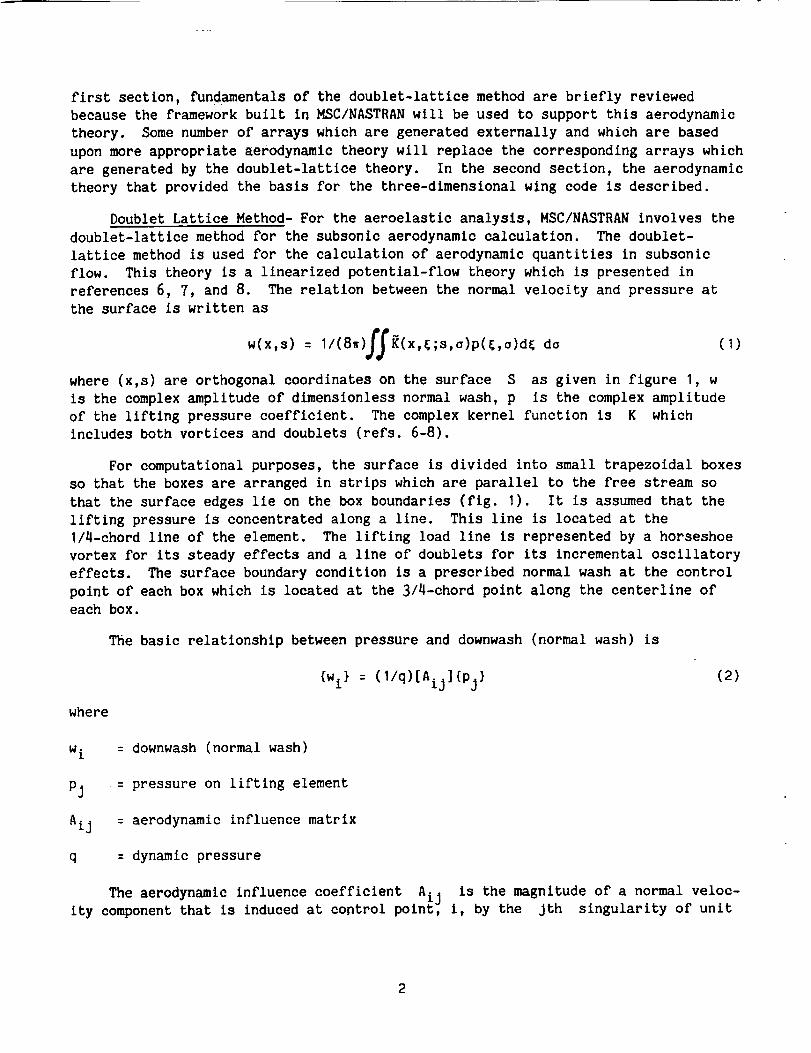
SUMMARY

A static aeroelastlc analysis capability that can calculate flexible air loads

for generic configuration aircraft was developed. It was made possible by integrat-

ing a finite element structural analysis code (MSC/NASTRAN) and a panel code of

aerodynamic analysis based on linear potential flow theory. The framework already

built in MSC/NASTRAN was used and the aerodynamic influence coefficient matrix is

computed externally and inserted In the NASTRAN by means of a DMAP program. It was

shown that deformation and flexible alrloads of an oblique wing aircraft can be

calculated reliably by this code both in subsonic and supersonic speeds. Prelimi-

nary results indicating importance of flexibility in calculating air loads for this

type of aircraft are presented.

INTRODUCTION

The objective of this research is to develop a general statlo-aeroelastic

analysis capability by integrating a panel code for aerodynamic analysis that can

cover subsonic as well as supersonic range for both symmetric and asymmetric config-

uration aircraft into a flnite-element structural analysis program. There is no

such capability available, except for those imbedded in the proprietary systems used

by aircraft manufacturers. In order to make the best use of available resources, a

decision was made to use the framework of the MSC/NASTRAN static-aeroelastic analy-

sis capability (refs. I-3) and to replace the aerodynamic analysis module with the

three-dimenslonal wing code (refs. 4, 5, and private communication of R. Carmichael

and I. Kroo), which is applicable to both the supersonic and the subsonic regime,

and includes modification to be able to predict the in-plane force caused by the

leading-edge suction. Consequently, the capabilities to perform flexible alrload

calculation and structural wing design for oblique wing aircraft are developed as

the results of this study. Various examples were solved to verify the capabilities

of the combined system, and program capabilities and limitations were identified.

STATIC AEROELASTICITY

Aerodynamic Theories

Static aeroelasticity is a problem that involves the response of a flexible

structure to aerodynamic loading. The analysis of static aeroelasticlty involves

calculation of static response, including loads and stresses in the structure. In

this section, the basic theories involved in this analysis are described. In the

first section, fundamentals of the doublet-lattice method are briefly reviewed

because the framework built in MSC/NASTRAN will be used to support this aerodynamic

theory. Some number of arrays which are generated externally and which are based

upon more appropriate aerodynamic theory will replace the corresponding arrays which

are generated by the doublet-lattice theory. In the second section, the aerodynamic

theory that provided the basis for the three-dimensional wing code is described.

Doublet Lattice Method- For the aeroelastic analysis, MSC/NASTRAN involves the

doublet-lattice method for the subsonic aerodynamic calculation. The doublet-

lattice method is used for the calculation of aerodynamic quantities in subsonic

flow. This theory is a linearized potential-flow theory which is presented in

references 6, 7, and 8. The relation between the normal velocity and pressure at

the surface is written as

w(x,s) : I/(8_)ffK(x,_;s,a)p(_,a)d_ do (I)

where (x,s) are orthogonal coordinates on the surface S as given in figure I, w

is the complex amplitude of dimensionless normal wash, p is the complex amplitude

of the lifting pressure coefficient. The complex kernel function is K which

includes both vortices and doublets (refs. 6-8).

For computational purposes, the surface is divided into small trapezoidal boxes

so that the boxes are arranged in strips which are parallel to the free stream so

that the surface edges lie on the box boundaries (fig. I). It is assumed that the

lifting pressure is concentrated along a line. This line is located at the

I/4-chord line of the element. The lifting load line is represented by a horseshoe

vortex for its steady effects and a line of doublets for its incremental oscillatory

effects. The surface boundary condition is a prescribed normal wash at the control

point of each box which is located at the 3/4-chord point along the centerline of

each box.

The basic relationship between pressure and downwash (normal wash) is

{wi} : (I/q)[Aij]{p j}(2)

where

w i : downwash (normal wash)

pj .: pressure on lifting element

Aij : aerodynamic influence matrix

q = dynamic pressure

The aerodynamic influence coefficient Aij is the magnitude of a normal veloc-

ity component that is induced at control point_ i, by the jth singularity of unit

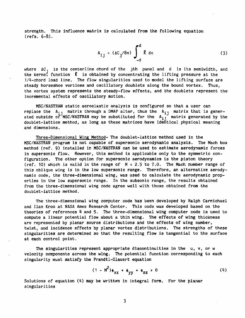
strength. This influence matrix is calculated from the following equation(refs. 6-8).

dAij = (ACjI8_) R dn

-d

(3)

where ACj is the centerline chord of the jth panel and d is its semiwidth, andthe kernel function _ is obtained by concentrating the lifting pressure at the

I/4-ohord load line. The flow singularities used to model the lifting surface are

steady horseshoe vortices and oscillatory doublets along the bound vortex. Thus,

the vortex system represents the steady-flow effects, and the doublets represent the

incremental effects of oscillatory motion.

MSC/NASTRAN static aeroelastlc analysis is configured so that a user can

replace the Aij matrix through a DMAP alter, thus the At._j matrix that is gener-

ated outside of MSC/NASTRAN may be substituted for the Aij matrix generated by the

doublet-lattice method, as long as these matrices have identical physical meaning

and dimensions.

Three-Dimenslonal Wing Method- The doublet-lattice method used in the

MSC/NASTRAN program is not capable of supersonic aerodynamic analysis. The Math box

method (ref. 9) installed in MSC/NASTRAN can be used to estimate aerodynamic forces

in supersonic flow. However, this method is applicable only to the symetric con-

figuration. The other option for supersonic aerodynamics is the piston theory

(ref. 10) which is valid in the range of M = 2.5 to 7.0. The Math number range of

this oblique wing is in the low supersonic range. Therefore, an alternative aerody-

namic code, the three-dimensional wing, was used to calculate the aerodynamic prop-

erties in the low supersonic range. In the subsonic range, the results obtained

from the three-dimenslonal wing code agree well with those obtained from the

doublet-lattice method.

The three-dimensional wine computer code has been developed by Ralph Carmlchael

and Ilan Kroo at NASA Ames Research Center. This code was developed based on the

theories of references 4 and 5. The three-dimensional wine computer code is used to

compute a linear potential flow about a thin wing. The effects of win E thickness

are represented by planar source distributions and the effects of wine camber,

twist, and incidence effects by planar vortex distributions. The strengths of these

singularities are determined so that the resulting flow is tangential to the surface

at each control point.

The singularities represent appropriate discontinuities in the u, v, or w

velocity components across the wing. The potential function corresponding to each

singularity must satisfy the Prandtl-Glauert equation

(1 - M2)¢xx + _yy + _zz = 0

Solutions of equation (4) may be written in integral form. For the planar

singularities

(4)

3

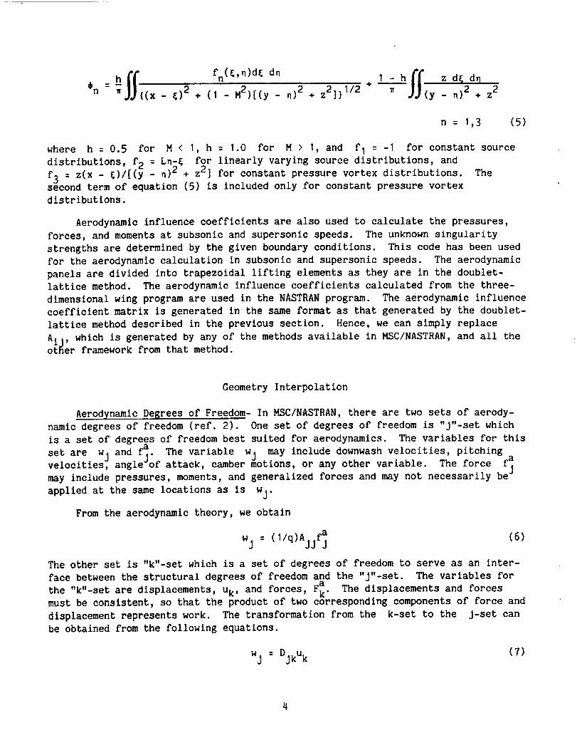
h ['_. fn({,n)d{ dn I - h _T z d{ dll

JJ " ,_J (y-n +zCn _ {(x - _,)2 + (1 - M2)[(y - n) 2 + z2]} 1/2 + )2 2

n = 1,3 (5)

where h : 0.5 for M < I, h : 1.0 for M > I, and fl : -I for constant source

distributions, f2 = Ln-{ for linearly varying source distributions, and

f3 = z(x - {)/[(y n)2 + z2] for constant pressure vortex distributions. Thesecond term of equation (5) is included only for constant pressure vortex

distributions.

Aerodynamic influence coefficients are also used to calculate the pressures,

forces, and moments at subsonic and supersonic speeds. The unknown singularity

strengths are determined by the given boundary conditions. This code has been used

for the aerodynamic calculation in subsonic and supersonic speeds. The aerodynamic

panels are divided into trapezoidal lifting elements as they are in the doublet-

lattice method. The aerodynamic influence coefficients calculated from the three-

dimensional wing program are used in the NASTRAN program. The aerodynamic influence

coefficient matrix is generated in the same format as that generated by the doublet-

lattice method described in the previous section. Hence, we can simply replace

Aij , which is generated by any of the methods available in MSC/NASTRAN, and all theotBer framework from that method.

Geometry Interpolation

Aerodynamic Degrees of Freedom- In MSC/NASTRAN, there are two sets of aerody-

namic degrees of freedom (ref. 2). One set of degrees of freedom is "j"-set which

is a set of degrees of freedom best suited for aerodynamics. The variables for this

and f_. The variable w_ may include downwash velocities, pitchingset are wj J a . avelocities, angle of attack, camber motions, or any other varzable. The force fl

may include pressures, moments, and generalized forces and may not necessarily be_

applied at the same locations as is wj.

From the aerodynamic theory, we obtain

wj : (I/q)Ajjf_(6)

The other set is "k"-set which is a set of degrees of freedom to serve as an inter-

face between the structural degrees of freedom and the "J"-set. The variables for

a The displacements and forcesthe "k"-set are displacements, Uk, and forces, Fk.

must be consistent, so that the product of two corresponding components of force and

displacement represents work. The transformation from the k-set to the j-set can

be obtained from the following equations.

wj : DjkU k (7)

4

a

Fk = Skj_j (8)

where

a : displacement and forces at aerodynamic grid pointsUk,F k

a = pressure on lifting elementfj

There are several ways of choosing the uk degrees of freedom. For each aerody-namic element, two displacements are chosen in the doublet-lattice method of

MSC/NASTRAN. Their locations are the center of pressure and the downwash center.

In the subsonic speed, the center of pressure is I/4 chord and the downwash center

is 3/4 chord. Thus, for the doublet-lattice method, the j-set is the downwash at

the 3/4 chord and the pressure, and the k-set is the normal displacement at the

center of pressure and the normal displacement at the downwash center. Two sets of

degrees of freedom are illustrated in figure 2 (ref. 2).

Here, the k-set consists of:

Uk1: normal displacement at center of pressure

Uk2: normal displacement at downwash center

and J-set consists of:

wj: downwash at downwash center

a

fj: pressure coefficient at center of pressure

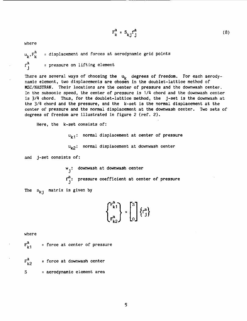
The Ski matrix is given by

t

where

Fakl

: force at center of pressure

Fak2

S

: force at downwash center

: aerodynamic element area

5

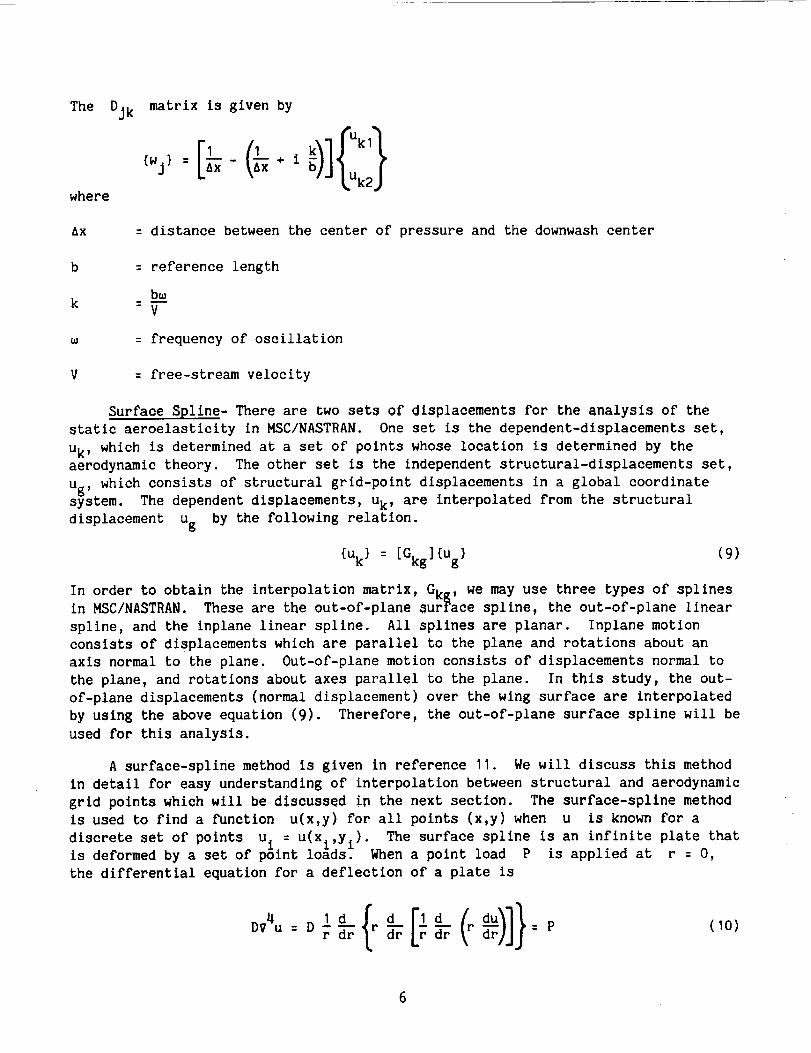
The Djk matrix is given by

where

AX : distance between the center of pressure and the downwash center

b = reference length

b_k

- V

: frequency of oscillation

V : free-stream velocity

Surface Spline- There are two sets of displacements for the analysis of the

static aeroelasticity in MSC/NASTRAN. One set is the dependent-displacements set,

Uk, which is determined at a set of points whose location is determined by the

aerodynamic theory. The other set is the independent structural-displacements set,

Ug, which consists of structural grid-polnt displacements in a global coordinatesystem. The dependent displacements, Uk, are interpolated from the structural

displacement Ug by the following relation.

{uk} : [Gkg]{Ug} (9)

In order to obtain the interpolation matrix, Gkg , we may use three types of splines

in MSC/NASTRAN. These are the out-of-plane surface spline, the out-of-plane linear

spline, and the inplane linear spline. All splines are planar. Inplane motion

consists of displacements which are parallel to the plane and rotations about an

axis normal to the plane. Out-of-plane motion consists of displacements normal to

the plane, and rotations about axes parallel to the plane. In this study, the out-

of-plane displacements (normal displacement) over the wing surface are interpolated

by using the above equation (9). Therefore, the out-of-plane surface spline will be

used for this analysis.

A surface-spline method is given in reference 11. We will discuss this method

in detail for easy understanding of interpolation between structural and aerodynamic

grid points which will be discussed in the next section. The surface-spline method

is used to find a function u(x,y) for all points (x,y) when u is known for a

discrete set of points u = u(x:,Yi). The surface spline is an infinite plate thatis deformed by a set of _int loads. When a point load P is applied at r = O,

the differential equation for a deflection of a plate is

DV4u : D r d-r _ d-r : P (I0)

6

where r represents a polar coordinate. A solution for the deflection of the plate

with many concentrated loads can be obtained by superimposing solutions of equation

(10)•

N

u(x,y) : b o + blx + b2Y + _ Ki(x,y)P i

i:I

(11)

where

Ki(x,Y)

2r.

1

P,

1

2 2= (1/16 '_D)r i _n r i

= )2(x i- x + (Yi- y)2

: concentrated load at (xi,Y i)

The N + 3

equations

unknowns (bo, bl, b2, Pi' i : I,N) can be obtained from the N + 3

Pi :0

_xiP i : 0

_yip i = 0

(12)

(13)

(14)

andN

uj : bo + blX j + b2Y j + _ Ki(xj,yj)P i

i=l

(j : 1,N) (15)

Here, K.(xlJ,YJ ) .-Kj(xi,Y i) and Ki(xl,y j) : 0 when i --T_e unknownsThe unknown variables,u are the displ_cements at the structural grid points•

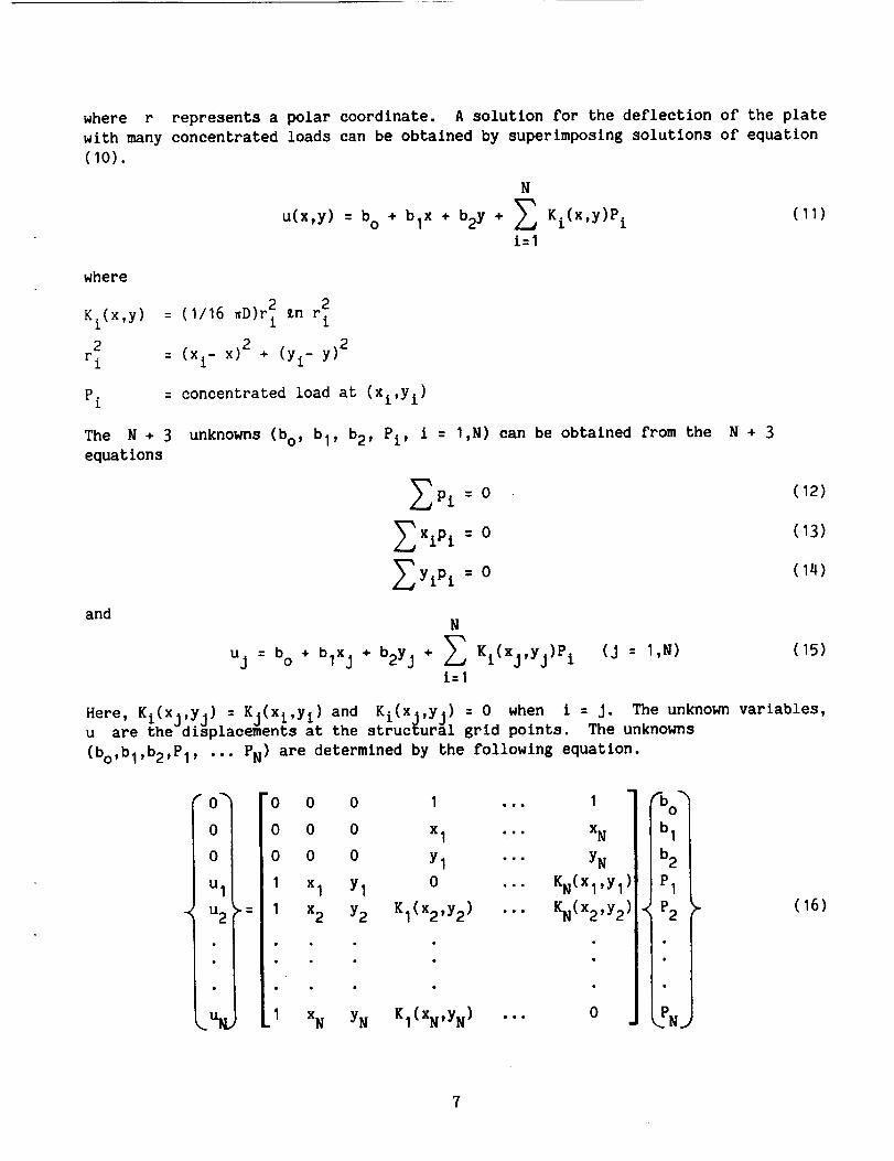
(bo,bl,b2,P1, ... PN ) are determined by the following equation•

o I

O l

ull

U2 i_'=

_,.ul¢,

"0

0

0

I

I

0 0 1 ... 1

0 0 x 1 ... xN

0 0 Yl "•• YN

Xl Yl 0 ..• KN(Xl,Y 1

x2 Y2 KI(x2'Y2) "'" KN(x2'Y2)

xN YN KI(XN'YN) "'" 0

0

b 1

b2

P1

"< P2

t"

,. (16)

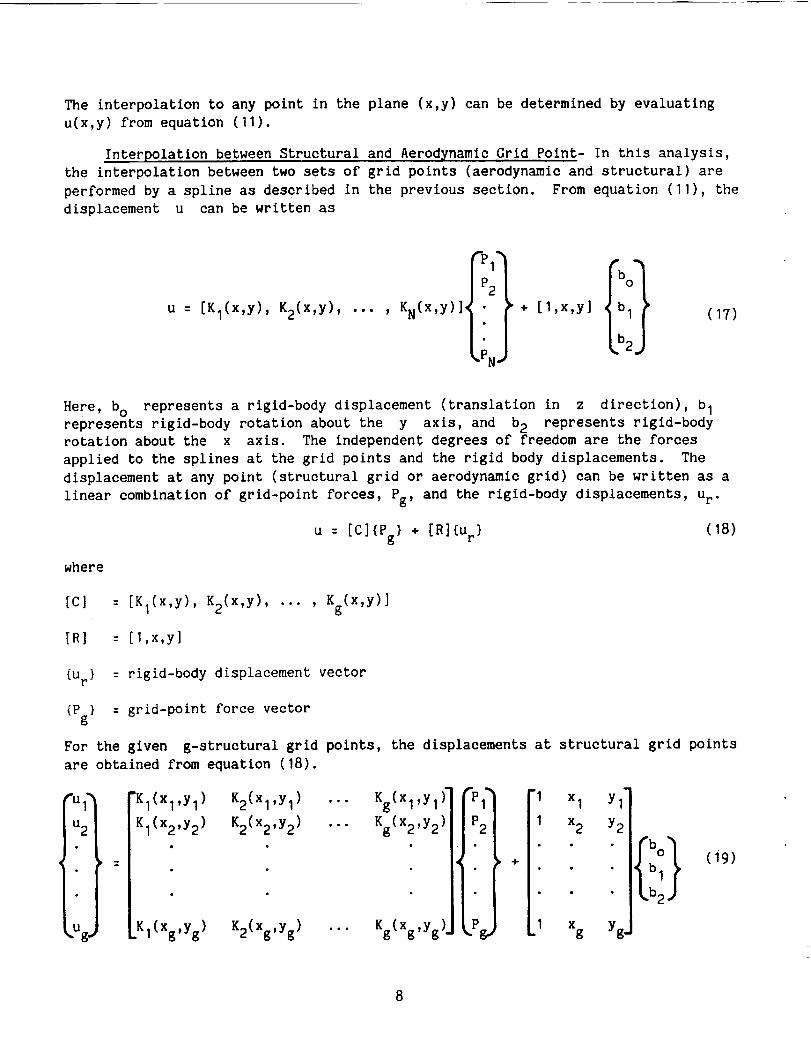
The interpolation to any point in the plane (x,y) can be determined by evaluatingu(x,y) from equation (11).

Interpolation between Structural and Aerodynamic Grid Point- In this analysis,

the interpolation between two sets of grid points (aerodynamic and structural) are

performed by a spline as described in the previous section. From equation (11), the

displacement u can be written as

u : [K1(x,y), K2(x,y), ... , KN(x,y)] I• + [1,x,y] , b 1• !

"PN" 2

(17)

Here, bo represents a rigid-body displacement (translation in z direction), b I

represents rigid-body rotation about the y axis, and b2 represents rigid-bodyrotation about the x axis. The independent degrees of freedom are the forces

applied to the splines at the grid points and the rigid body displacements. The

displacement at any point (structural grid or aerodynamic grid) can be written as a

linear combination of grid-point forces, Pg, and the rigid-body displacements, ur.

u : [C](Pg} + [R](u r}(18)

where

[c] : [K1(x,y) , K2(x,y) , ... , Kg(x,y)]

[R] : [1,x,y]

{ur} = rigid-body displacement vector

{Pg} = grid-point force vector

For the given g-structural grid points, the displacements at structural grid points

are obtained from equation (18).

.uq

• I

I

"KI(Xl,Y I)

KI(x2,Y 2)

.K1(xg,Yg)

K2(xl,Y I) ... Kg(Xl,Y1_

K2(x2,Y 2) ... Kg(X2,Y 2)

K2(xg,yg) ... Kg(Xg,yg).

1"IIIP21

• ? +

ii"

g_

"1 x 1

1 x2

1m

Xg

Yl

Y2

fbo}b 1

b2

Yg

(i9)

or

{Ug} = [Cgg]{Pg} + [Rg]{U r} (20)

If the angular displacements are included in equation (18), the C matrix should be

modified. From equations (12), (13), and (14), the equilibrium equations for the

structural grid points are

I I

xI x2

Yl Y2

• • g ]XgYg

ii

= (0}I

I

(21)

This equation can be rewritten as

[R_](Pg} = o

Thus, for the structural grid points, the following equations are obtained.

(22)

re<< (23)

For k aerodynamic grid points, the displacement can be given in terms of the

structural grid-point forces, Pg and the rigid body displacement, ur. Thus, fromequation (18),

1112

KI(Xl,Y 1) K2(xl,Y 1) ... Kg(Xl,Yl)"

KI(x2,Y 2) K2(x2,Y 2) ... Kg(x2,Y 2)

,KI(Xk,Y k) K2(Xk,Y k) ... Kg(Xk,Yk) ,

"PI"

P2

i p

"I xI YI"

I x2 Y2

.1 x k Yk

b 1

2

(24)

Or

{uk} : [Ckg](Pg} + [Rk](U r}(25)

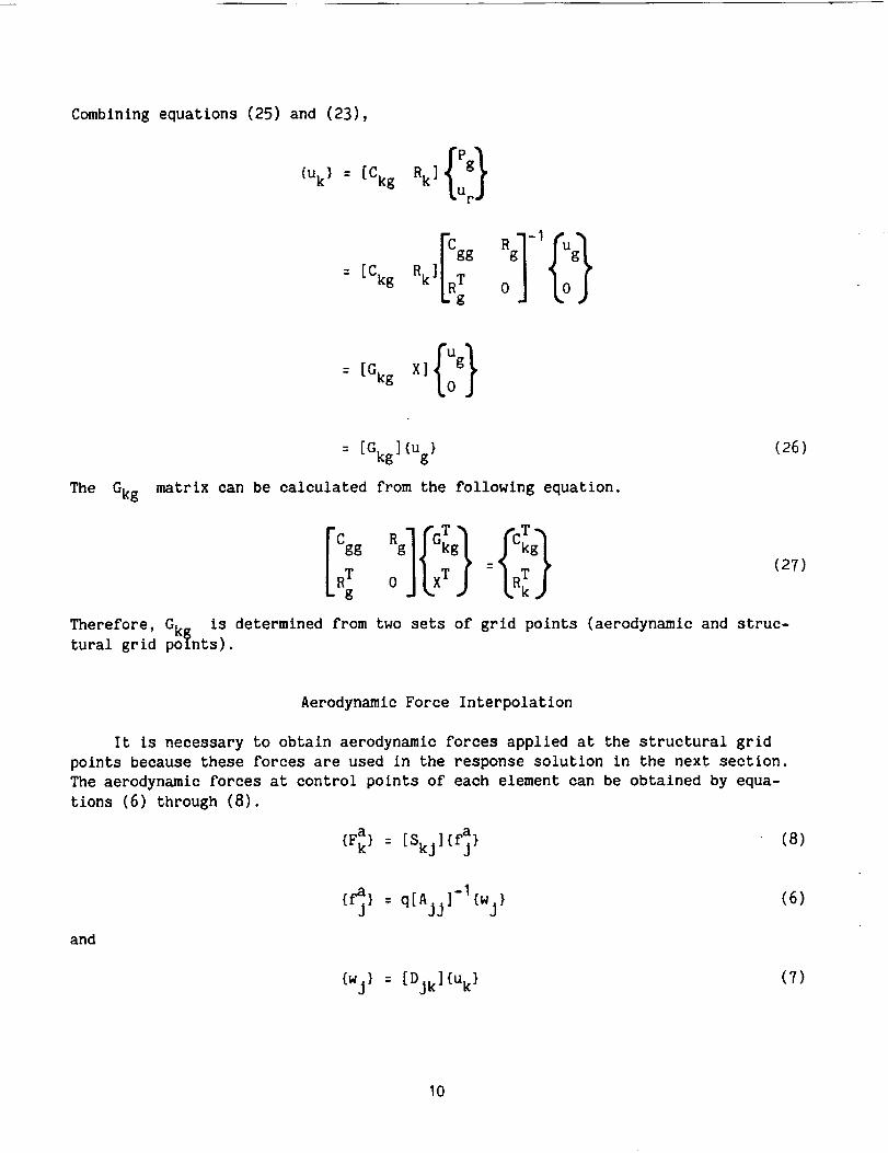
Combining equations (25) and (23),

{Uk} : [Ckg Rk]_]IPg_

tJur

rcg

The Gkg

: [Gkg](Ug}

matrix can be calculated from the following equation.

(26)

Cgg(27)

Therefore, Gk_ is determined from two sets of grid points (aerodynamic and struc-tural grid points).

Aerodynamic Force Interpolation

It is necessary to obtain aerodynamic forces applied at the structural grid

points because these forces are used in the response solution in the next section.

The aerodynamic forces at control points of each element can be obtained by equa-

tions (6) through (8).

Fa {f_}{ k} : [Skj]

{f_j} : q[Ajj]-1{wj}

and

{wj} : [Djk]{U k}

(8)

(6)

(7)

10

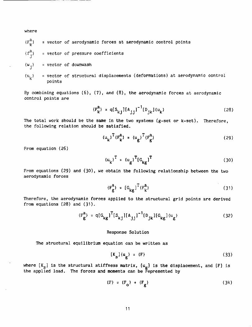
where

(F_}

{f j}

{wj}

{uk}

: vector of aerodynamic forces at aerodynamic control points

= vector of pressure coefficients

= vector of downwash

= vector of structural displacements (deformations) at aerodynamic control

points

By combining equations (6), (7), and (8), the aerodynamic forces at aerodynamic

control points are

{F_} : q[Skj][Ajj]-1[Djk]{Uk }

The total work should be the same in the two systems (g-set or k-set).

the following relation should be satisfied.

{uk}T{Fk} : {ug}T{Fg}

From equation (26)

(28)

Therefore,

(29)

(uk}T : {ug}T[Gkg]T (30)

From equations (29) and (30), we obtain the following relationship between the two

aerodynamic forces

: G -T aFa} [ } (31){ g kg j {Fk

Therefore, the aerodynamic forces applied to the structural grid points are derived

from equations (28) and (31).

{Fg}a : q[Gkg]T[Skj][Ajj]-|[Djk][Gkg]{Ug } (32)

Response Solution

The structural equilibrium equation can be written as

[Ks](Ug} = {F} (33)

where [Ks] is the structural stiffness matrix, {Ug} is the displacement, and [F] isthe applied load. The forces and moments can be represented by

{F} : {Fo} + {Fg} (34)

11

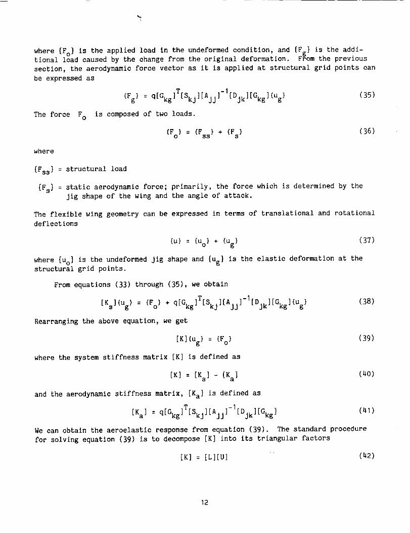
where {Fo} is the applied load in the undeformed condition, and {F_} is the addi-5tional load caused by the change from the original deformation. From the previous

section, the aerodynamic force vector as it is applied at structural grid points can

be expressed as

The force Fo

{Fg} : q[Gkg]T[Skj][Ajj]-1[Djk][Gkg]{Ug}

is composed of two loads.

{Fo} : {Fss} + {Fs}

(35)

(36)

where

{Fss } = structural load

{Fs] = static aerodynamic force; primarily, the force which is determined by the

Jig shape of the wing and the angle of attack.

The flexible wing geometry can be expressed in terms of translational and rotational

deflections

{u} = {uO} + {Ug} (37)

where {uo] is the undeformed jig shape and {Ug} is the elastic deformation at the

structural grid points.

From equations (33) through (35), we obtain

[Ks]{Ug } = {Fo} + q[Gkg]T[Skj][Ajj]-1[Djk][Gkg]{Ug} (38)

Rearranging the above equation, we get

[K]{Ug} = {Fo} (39)

where the system stiffness matrix [K] is defined as

[K] : [Ks ] - [Ka] (40)

and the aerodynamic stiffness matrix, [Ka] is defined as

q[Gkg]T[Skj I[Ka] = ][Ajj]- [Djk][Gkg] (41)

We can obtain the aeroelastic response from equation (39). The standard procedure

for solving equation (39) is to decompose [K] into its triangular factors

[K] = [L][U] (42)

12

where [L] is a lower triangle with unit elements on the diagonal and [U] is an upper

triangle. Then, equation (39) can be rewritten as

[L]{y} : {Fo} (43)

and

[U]{Ug} = {y} (44)

The solution of equation (43) for {y} is obtained by the forward substitution, and

the subsequent solution of equation (44) is obtained by the backward substitution.

The above solution may require a significant amount of computer time because

the aerodynamic stiffness matrix [Ka] is relatively full, when compared to [Ks].

such cases, an iterative procedure may be more efficient. From equation (39), we

can formulate the iteration procedure.

where {u_} is thenth

[Ks]{U _} = {Fo} + [Ka]'un-1}tg

iterate.

In

(45)

RESULTS AND DISCUSSION

Sample Problems

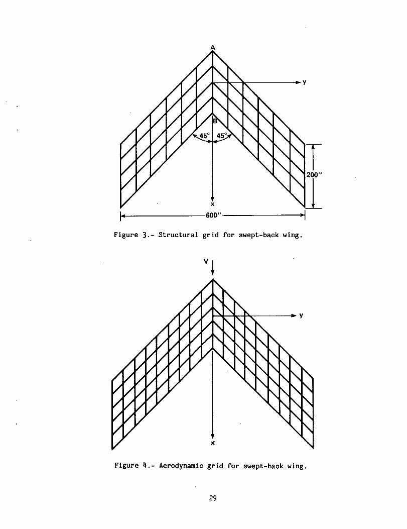
Swept-Back Wing- As a first problem, a 45 ° swept-back flat-plate wing has been

analyzed. The structural elements and aerodynamic elements are shown in figures 3

and 4, respectively. The structural and aerodynamic panels are both two-

dimensional. The wing span is 600 in. and its chord length is 200 in. The struc-

tural thickness of the aluminum wing plate is 2 in.; however, aerodynamically the

wing is assumed to be a thin panel. In this case, the dynamic pressure is 2 psi and

the angle of attack is 10° .

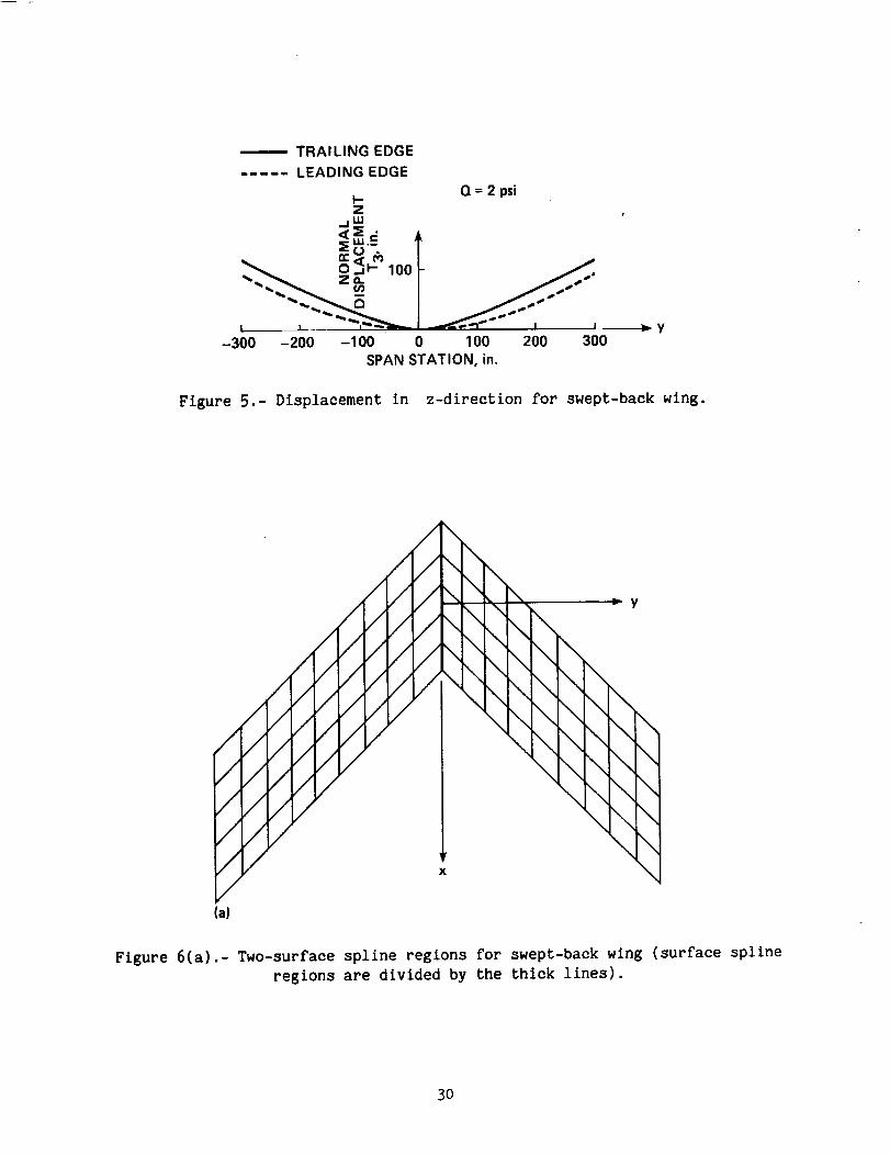
The clamped boundary condition is given along a line AB in figure 3. The

structural displacements are given in figure 5. Because of the symmetric air load-

ing, the displacements in the z-direction are symmetrical with respect to x-z

plane. The trailing edge has more deflection than the leading edge does since the

wing has a larger moment arm about the reference pitch axis near the trailing edge.

The aerodynamic forces have been calculated with the doublet-lattice method

installed in MSC/NASTRAN and also with the aerodynamic influence coefficients

obtained by using the three-dimensional wing program. Throughout this report, the

doublet-lattice method has been used to calculate the subsonic aerodynamic quanti-

ties. The three-dimensional wing code was shown to be a reliable computer code by

comparing its results and those of the doublet lattice code, and it has been used

exclusively to calculate supersonic aerodynamic quantities. The results of the two

13

analyses virtually agreed. The comparison between two results is given in the

section on the 250-ft 2 oblique wing.

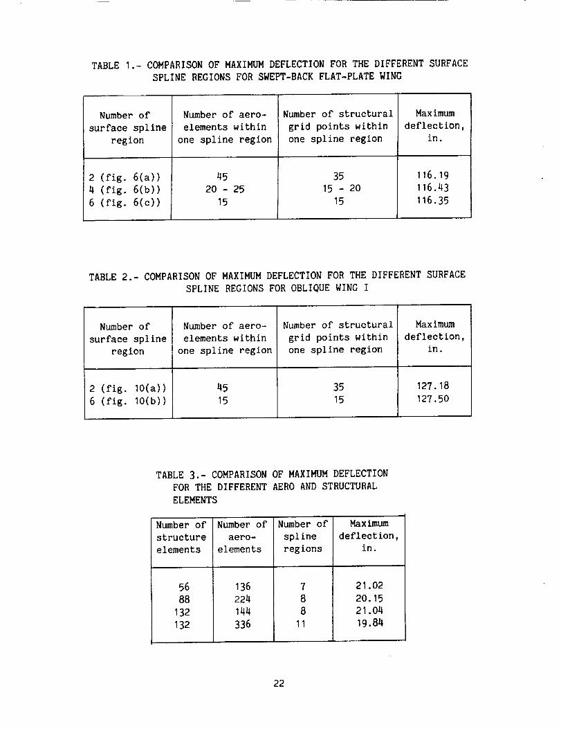
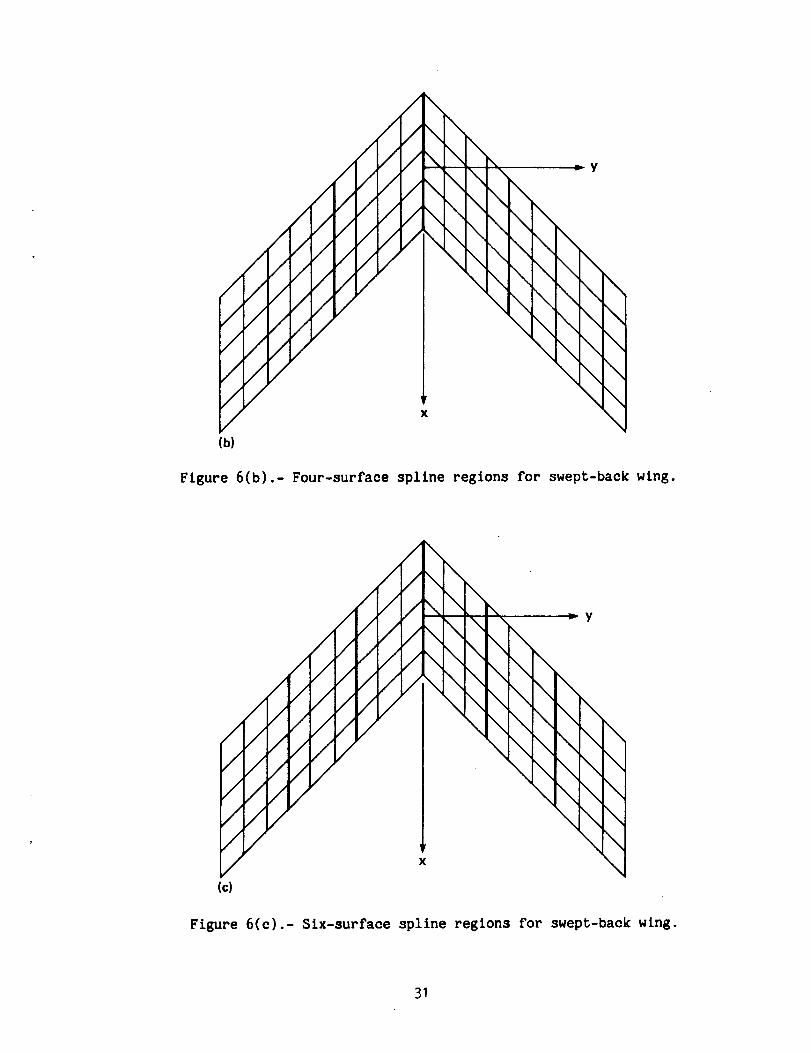
Table I gives the accuracy for several different interpolation regions. In the

appendix, the interpolation regions are explained. Figure 6 shows the surface-

spline regions used in this analysis. Figure 6(a) shows 2 spline regions, fig-

ure 6(b) shows 4 regions, and figure 6(c) shows 6 regions. The maximum difference

for the maximum deflection is only 0.2% for the above cases. Therefore, the number

of aerodynamic elements in a surface-spline region does not significantly affect the

results.

Oblique Wing-I- As a second problem, a simple, asymmetric flat-plate wing with

a sweep angle of 45 ° has been analyzed. This wing has been chosen as a preliminary

model for a more complicated oblique wing.

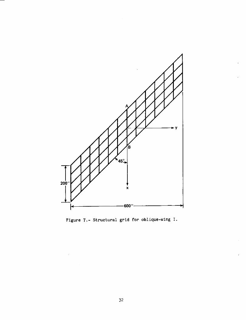
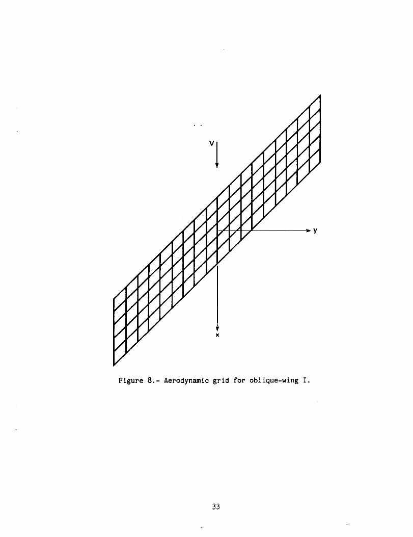
The structural and aerodynamic elements are shown in figures 7 and 8, respec-

tively. Both the structural and aerodynamic panels are two-dimensional with a wing

span of 600 in. and a chord length of 200 in. As in the previous case, the aluminum

plate thickness is 2 in. In this case, the dynamic pressure is 0.3 psi and the

angle of attack is 10°.

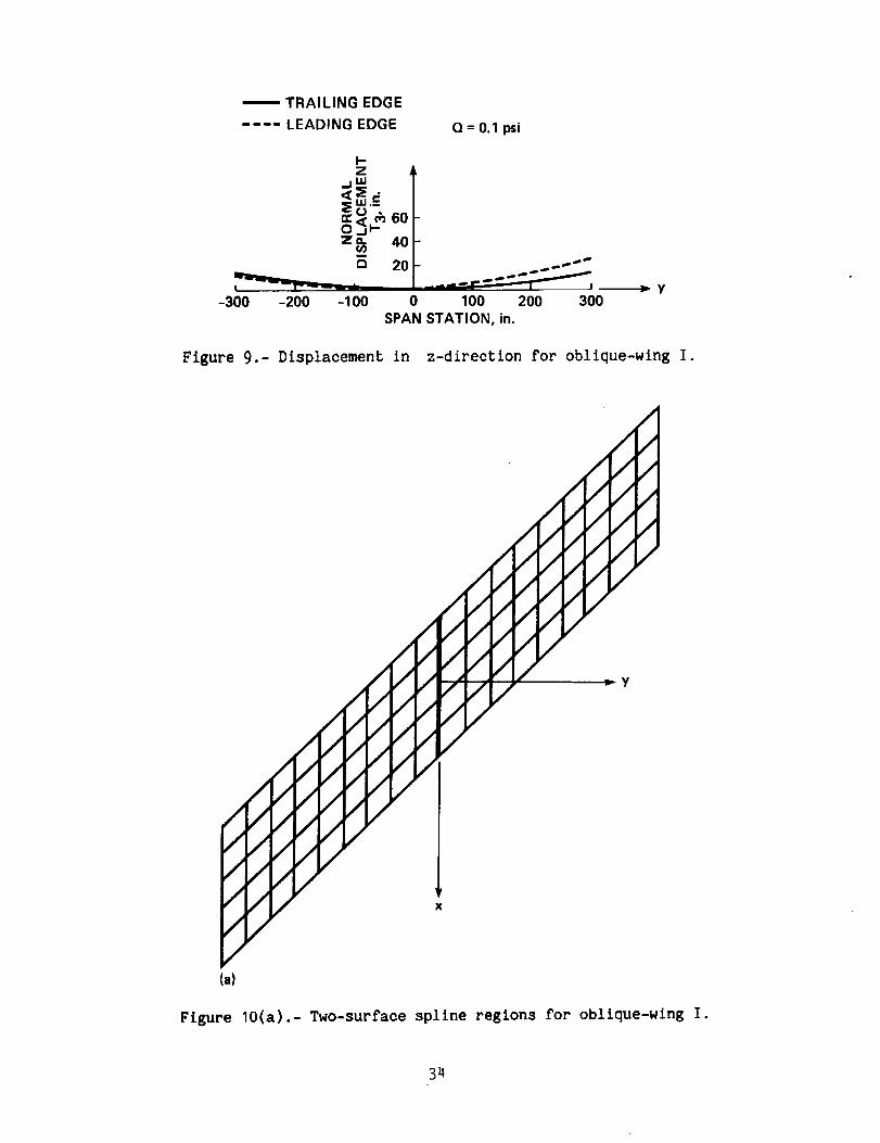
The clamped boundary condition is along line AB in figure 7. The structural

displacements are given in figure 9. The left-side wing has more loading than the

right-side wing does because the left-slde wing has more upwash than the right-side

wing. However, the right-side wing has more pitching moment about the y-axis than

the left-side wing does because the bigger loads are applied near the leading edge

of the wing. Therefore, the displacement pattern of the oblique wing is quite

different from that of the swept-back wing. The right wing is twisted to increase

the local angle of attack whereas the left wing is twisted to decrease the local

angle of attack.

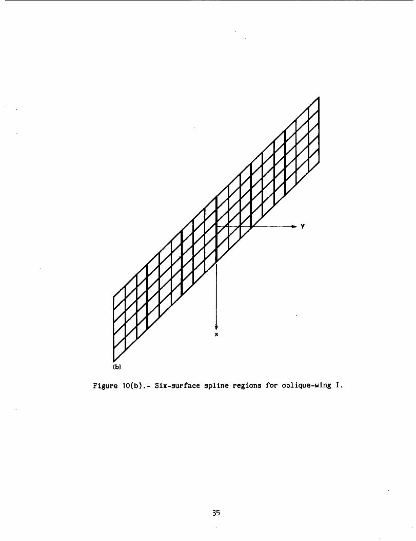
Table 2 gives the accuracy for two different interpolation regions. Figure 10

shows the spline regions used in this analysis. Figure IO{a) shows 2 spline

regions, and figure IO(b) shows 6 regions. The maximum difference for the maximum

deflection is only 0.25% for the above cases. Therefore, as seen before, the number

of aerodynamic elements in a surface-spline region does not significantly affect the

results.

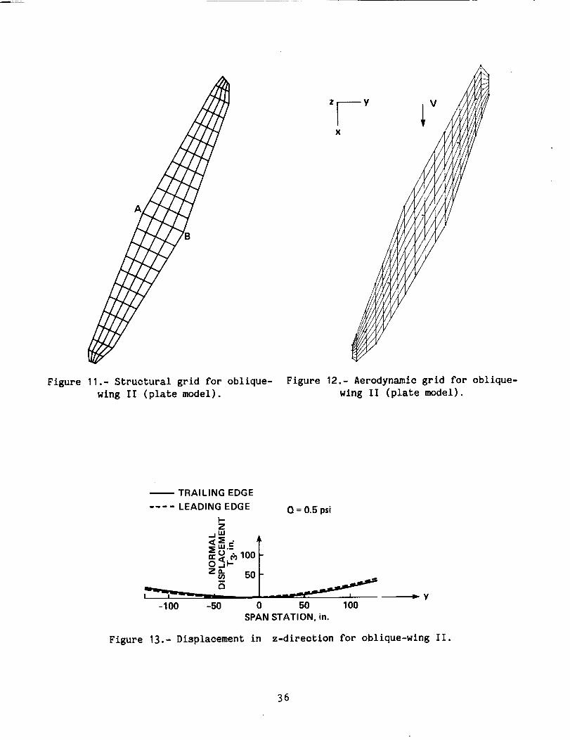
Oblique Wing-II- As a third problem, another two-dlmensional oblique wing with

total area of 250 ft2 has been analyzed. Several different numbers of aerodynamic

and structural elements (table 3) are used for the calculation. Among them, the

typical structural elements and aerodynamic elements are given in figures 11 and 12,

respectively. Both the structural and aerodynamic panels are two-dimensional. The

aluminum plate thickness is again 2 in. In this case, the dynamic pressure is

0.5 psi and the angle of attack is 10°.

The clamped boundary condition is along line AB in figure 11. The structural

displacements are given in figure 13. As in the ease for the oblique wing I, the

left-side wing has more lift than does the right-side wing. However, the wing tip

14

of the right-side wing has more deflection than the left-side wing does because of

the different moment pattern. The general deflection pattern for this wing is

similar to that for the previous case.

Table 3 shows the relation between the maximum deflection and the number of

aerodynamic and structural elements. The number of aerodynamic elements affects

structural deformation more significantly than does the number of structural ele-

ments. For almost the same number of aerodynamic elements (136 and 144), the maxi-

mum deflection is almost the same (only O.1% difference) when increasing the number

of structural elements (from 56 to 132). Maximum deflection occurs at the tip of

the right-side wing. However, the maximum deflection decreases by 4.2% when

increasing the number of aerodynamic elements from 144 to 224, also decreases by

5.7% when increasing the number of aerodynamic elements from 144 to 336. We can see

that the more aerodynamic elements there are, the more accurate the prediction is

for aerodynamic forces over the wing surface. Therefore, we should have enough

aerodynamic elements to predict the correct aerodynamic forces. Near the leading-

edge and wing-tlp regions, the pressure variations are very steep, and fine'aerody-

namic meshes are required.

Figure 14(a) shows 7 surface-spline regions where the number of aeroelements is

136 and figure 14(b) shows 11 surface-spline regions where the number of aeroele-

ments is 336.

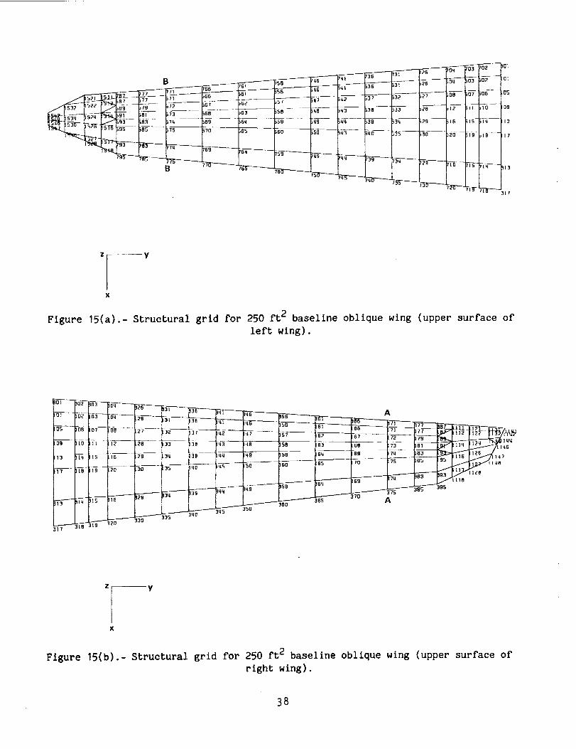
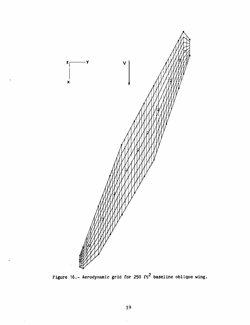
Oblique Wing (250 ft2)

In this section, we will discuss the full-scale 250-ft 2 oblique wing. Also, we

will examine a rigid oblique wing and flexible-optimlzed wing to show the wing

flexibility effect. The structural elements of the upper surface are shown in

figures 15(a) and 15(b). The aerodynamic elements are given in figure 16. The

analyzed structural shape is three-dlmenslonal. For the aerodynamic analysis, zero-

thickness panels are used. However, the total lift will not be very different from

that obtained by three-dimensional aerodynamic calculation because the wing is a

thin airfoil. The thickness ratio of the airfoil at the centerline is 14% and

linearly decreases to 12% at the 85% semispan station. The sweep angle of the wing

is 65 °

Baseline Oblique Wing (250 ft2) - As a first problem for the full-scale oblique

wing, we consider an oblique wing of which the area is 250 ft2. The pln-Jolnted

boundary conditions are given at the four structural grid points. These points are

structural grid numbers 202, 219, 602, and 619, and they are located on the lower

surface of the wing. The corresponding structural grid numbers on the upper surface

are 102, 119, 502, and 519 and are shown in figures 15(a) and 15(b).

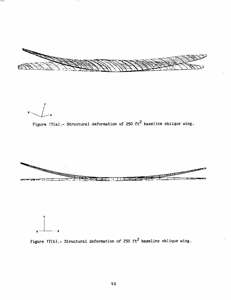
The structural deformations are shown in figures 17(a) and 17(b). Figure 17(a)

gives a three-dimenslonal view and figure 17(b) shows another view of oblique

wing. As in the previous case, the rlght-slde wing has more displacements than the

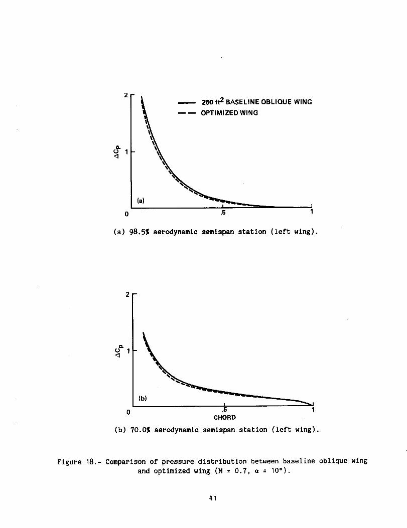
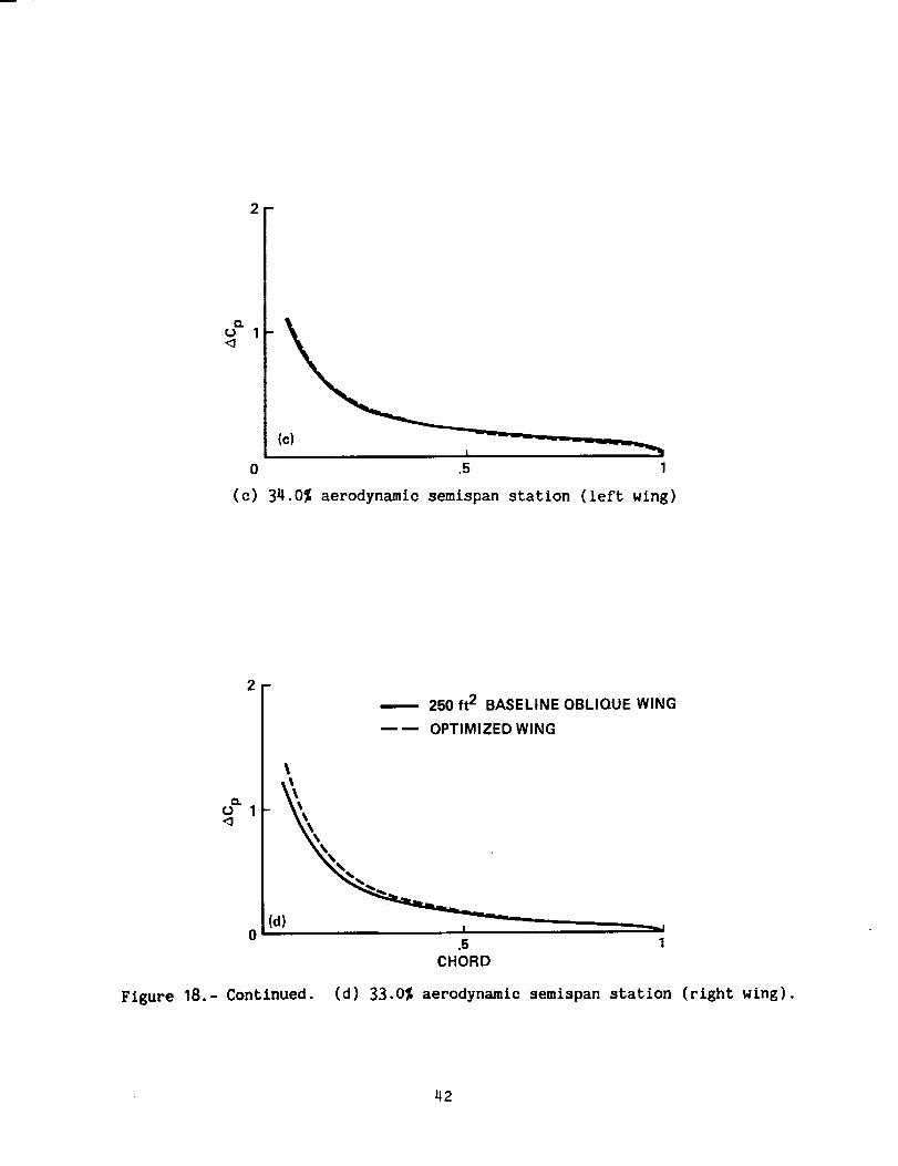
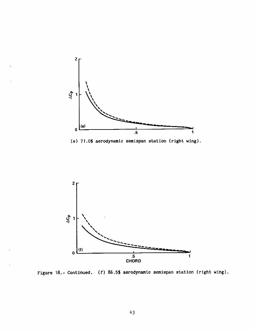
left-side wing. The aerodynamic pressure distributions are given in figure 18.

Here, the pressure is a differential pressure (lower surface pressure-upper surface

pressure). Near the leading edge, the high pressures are developed. In the case of

15

the rigid wing, the left-side wing has more lift than the right-side wing doesbecause the left-side wing is subjected to the stronger upwashwhich is developed bythe right-side wing. In this case, the Machnumber is 0.7 and the angle of attackis 10° . The solid curve represents pressure distributions of the baseline obliquewing, and the dashed curves represent pressure distributions of the optimized wingwhich is more flexible than the baseline wing. For the left-side wing, the baselinewing has more loading than the optimized (flexible) wing does. However, for theright-side wing, the optimized wing has more loading than the baseline wing does.The difference in loading pattern causes a change in the rolling moment, andreflects the wing's flexibility.

The comparison between the doublet-lattice method and the three-dimensionalwing program results is given in table 4. The total lift is almost the samebetweenthe two methods (0.4% differences). However, the maximumdeflection has moredifference (5.5%). The rolling-moment coefficient has somedifference but thesevalues are relatively small. For the interpolation of structural displacements, 11surface-spline regions are used. The surface spline regions are shown infigure 14(b).

Table 5 gives subsonic characteristics of the oblique wing according to the

various Mach numbers (0.4, 0.5, 0.6, and 0.7) at a fixed angle of attack (I0°).

Here, the load factors are calculated based on the value of aircraft gross weight as

24,000 lb. The lift coefficient changes are very small in the subsonic region.

Compared with the results of the rigid wing given in the section on the rigid wing,

the lift coefficient of this wing is slightly larger than that of the rigid wing.

The rolling-moment coefficient increases with the increase in the Mach number.

These two effects can be explained by the wing flexibility. We will discuss these

flexibility effects in the section on the rigid wing and the optimized wing. As

expected, the maximum vertical deflection increases when the lift force increases

and occurs at the tip of the right-side wing.

Table 6 shows the results for the three different angles of attack. The calcu-

lated angles of attack are 4.22, 10, and 15°. For this range of angle of attack,

the lift curve is in the linear region. The rolling-moment coefficient also

decreases linearly with the angle of attack. We can see the maximum deflection

varies almost linearly with the angle of attack.

Table 7 shows supersonic characteristics of the oblique wing. The aerodynamic

influence coefficients are calculated from the three-dimenslonal wing computer

code. In this supersonic speed, the sign of rolling moment changes from negative to

positive. That is, because of the wing-flexibility effect, the right wing has more

lift than the left wing. The angle of attack of the right wing (sweep-forward wing)

increases whereas that of the left wing (sweep-backward wing) tends to decrease.

Rigi d Wing- Table 8 gives the rigid-wing characteristics for the oblique

wing. The rigid-wing results were obtained by increasing E (Young's modulus) and

G (Shear modulus) by 100 times. For this rigid wing, both the lift coefficients and

rolling-moment coefficients are nearly constant with the increase in the Mach num-

ber. Therefore, we can say that there is no flexibility effect in this case.

16

Table 9 shows the rigid-win E results for the three different angles of

attack. The calculated angles of attack are 4.22, I0, and 15 °. For this range of

angle of attack, the lift curve is in the linear region. However, the lift-curve

slope decreases with the increase of wing rigidity as expected. The rolling-moment

coefficient also decreases linearly with the angle of attack.

Optimized Wing- In this section, we will discuss a strength-designed wing to

show the significant static aeroelastic effects on the wing displacements and the

aerodynamic quantities. The 250-ft 2 oblique wing described in the section on the

baseline oblique wing has been analyzed to show that it can withstand the composite

thickness for 4-g maneuvering condition. The criteria are applied to longitudinal

and shear strains for each of the 0, 45, and 90 ° piles. No stability criteria were

considered. The optimum composite wing-plate thickness distributions are given in

table 10. Span station I is the location number for the panel near the wing root

and span station 14 is for the panel near the wing tip. The structural elements and

aerodynamic elements are the same as those for the 250-ft 2 baseline oblique wing

given in the previous section.

Table 11 shows the static aeroelastic effects for the oblique wing. In this

case, the angle of attack is 15° and the Math number is 0.7. The 250-ft 2 oblique

win E has 2.3% more lift than the rigid wing does and the optimized wing has 7.8%

more lift than the rigid win E . There is a significant change in the deflection of

the optimized wing. The maximum deflection is 34.22 in. for the optimized wing and

it is 14.66 in. for the unoptimized wing (baseline 250-ft 2 wing). The rolling-

moment coefficient is positive for the optimized (flexible) wing and is negative for

the others. The big change in this coefficient shows the significance of wing

flexibility on aerodynamic load distribution.

Table 12 gives the subsonic characteristics for the optimized wing. The lift

coefficients are no longer constant for this flexible wing. With the increase of

the Math number (dynamic pressure), both the llft coefficient and rolling-moment

coefficient increase. This reflects the wing flexibility again. Between the Math

number, 0.5 and 0.6, the sign of rolling-moment coefficient changes from negative to

positive.

Discussions on Oblique Wing Analysis

Aerodynamic Coefficients- In this section, the previous results are

sun_,arized. Figure 19 shows the lift coefficient versus the Mach number in the

subsonic region. The sea level conditions are used for the calculations. The angle

of attack is I0° and the optimized (flexible) win E has the biggest lift. The

flexibility effects increase with the increase of Math number for both the baseline

oblique win E and the optimized wing. When the Math number is O.7, the lift

coefficient of the optimized wine is 7.8% higher than that of the rigid win E and the

coefficient of the baseline oblique wing is 5.4% higher than that of the rigid wing.

17

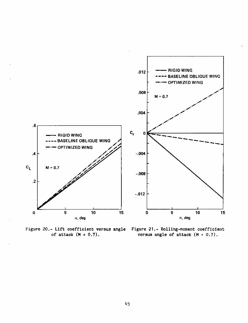
Figure 20 shows the lift-curve slopes for three wings at a Mach number of

0.7. Although the wing is flexible, the lift coefficient is still linear for this

range of angle of attack. The most flexible wing has more lift than the others as

expected.

Figure 21 shows the rolling-moment coefficient versus the angle of attack. The

calculated Mach number is 0.7. The rolling-moment coefficients are negative for

both the baseline oblique wing and the rigid wing, and they are positive for the

optimized (flexible) wing. The rolling-moment coefficients are also linear for this

range of angle of attack. For the optimized wing, wing flexibility gives a large

change in the rolling moment which is attributed to the increase of the local angle

of attack in the right-side wing, and the decrease of local angle of attack in the

left-side wing. One example for the local angle of attack calculation is given for

both the baseline oblique wing and the optimized wing in the next section.

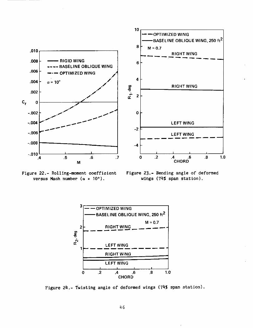
Figure 22 shows the rolling moment coefficient versus the Mach number. The

angle of attack is I0°. Substantial differences in the rolling moment caused by

wing flexibility are observed. For the rigid wing, the rolling moments are almost

constant but they tend to decrease slightly with the increase of Mach number. For

this rigid wing, the effective angle of attack is strongly affected by the upwash.

As we explained in the previous section, the upwash of the left-side wing (swept-

back wing) is larger than that of the right-side wing (swept-forward wing). This

effect results in the negative rolling moment for the rigid wing. As the angle of

attack increases, this upwash effect increases and the rolling moment decreases for

the rigid wing as illustrated in figure 21. We can see the same effect in fig-

ure 20. As the Mach number increases, the rolling moment decreases slightly for the

rigid wing.

Local angle of attack- In this section, we will discuss the local angle of

attack change caused by the change of wing bending as well as torsion to examine the

local effect of flexibility. For the flexible wing, depending on the span and chord

position of the wing, both torsion and bending angles vary. The magnitude of the

bending angle is maximum at the wing tip. We now examine the local angle-of-attack

change at the 74% semispan station in the structural coordinates for both the right-

side and the left-side wings. These span stations are shown in figure 15(a) (sec-

tion B-B) and in figure 15(b) (section A-A). The Mach number is 0.7 and RI is the

bending angle, or rotation about the x-axis and R2 is the twisting angle, or

rotation about the y-axis where the x and y axes are defined in the structural

coordinates. The positive bending angle occurs when the right-side wing is up and

the left-slde wing is down. Also, the positive twisting angle occurs when the wing

is in the positive pitch angle (nose-up).

Figure 23 shows the bending angle, RI at the given 74% semispan station. The

optimized wing has a bigger bending angle than the baseline oblique wing. For the

optimized wing, the magnitude of the bending angle of the right-side wing is more

than two times higher than that of the left-side wing. For the general wing struc-

ture, the magnitude of bending angle is bigger than that of the twisting angle at a

given wing position. For this high-sweep angle (65°), this big bending angle

results in the big change of local angle of attack.

18

Figure 24 shows the twisting angle, R2 at the 74% semispan station. As

expected, the optimized wing has more twisting angle than the baseline oblique

wing. The ,_gnitude of the twisting angle of the right-side wing is nearly two

times more than that of the left-side wing for the optimized wing and is 30 to 40%

more than that of the left-side wing according to the chord position for the base-

line oblique wing.

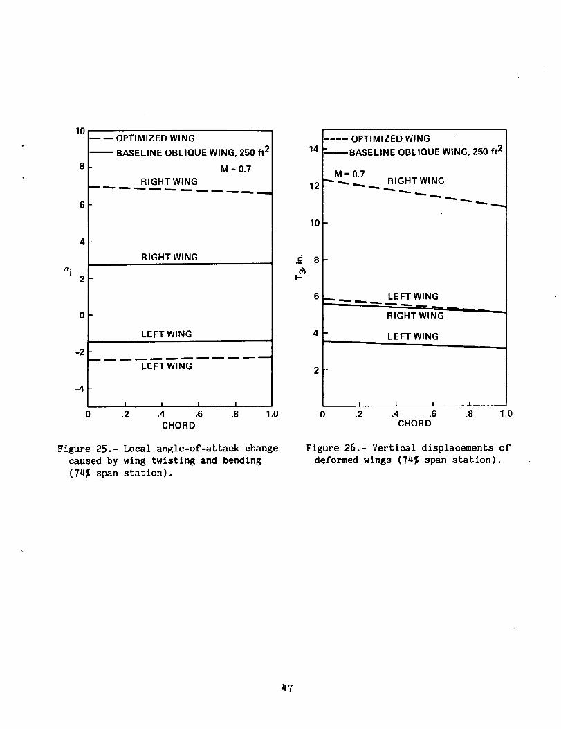
From these two angles, we can calculate the local angle-of-attack change. The

local angle of attack change, _i, is

ai = RI sin A + R2 cos A

where ^ is the wing sweep angle. Figure 25 shows the local angle-of-attack

change. The given angle of attack is 10°. At 74% semispan station, the local angle

of attack of the right-side wing is around 12.7° and that of the left-side wing is

around 8.6 ° for the baseline oblique wing. For the same span station of the opti-

mized wing, the local angle of attack of the rlght-side wing is about 16.8 ° and that

of the left-side wing is about 7.6 °. This difference in the angle of attack results

in the positive rolling moment for the optimized wing. Thus, the flexibility of

wing makes the significant difference in the local angle of attack and aerodynamic

characteristics and especially for the rolllng-moment characteristics.

Figure 26 shows the vertical displacement, T3 at the 74% semispan station.

The vertical displacement of the right-side wing is more than two times bigger than

that of the left-side wing in the optimized wing. For the same span station of the

baseline oblique wing, this displacement of the right-side wing is about 60% bigger

than that of the left-side wing.

CONCLUSIONS

A static-aeroelastie analysis capability has been developed that is applicable

to unsymmetric aircraft configuration including the oblique wing for both subsonic

and supersonic regimes.

Signlficances of wing flexibility are analyzed for the three different oblique

wings (very rigid wing, 250-ft 2 baseline wing, and optimized flexible wing). The

aerodynamic influence coefficients are calculated using both the doublet-lattice

method and the three-dimensional wing computer code to obtain the aerodynamic

forces. These two results are very close and are considered very reliable for

similar applications.

The supersonic capability for static aeroelastlcity has been developed by

combining the three-dimenslonal wing program and the MSC/NASTRAN computer program.

The increase of the number of aerodynamic elements affects the structural

deformation results more significantly than the increase of the number of structural

elements does.

19

The wing flexibility changes the local angles of attack, the load distribution

over the entire wing, and has the most significant effects on the rolling moment.

APPENDIX

INTERPOLATION PROCEDURE

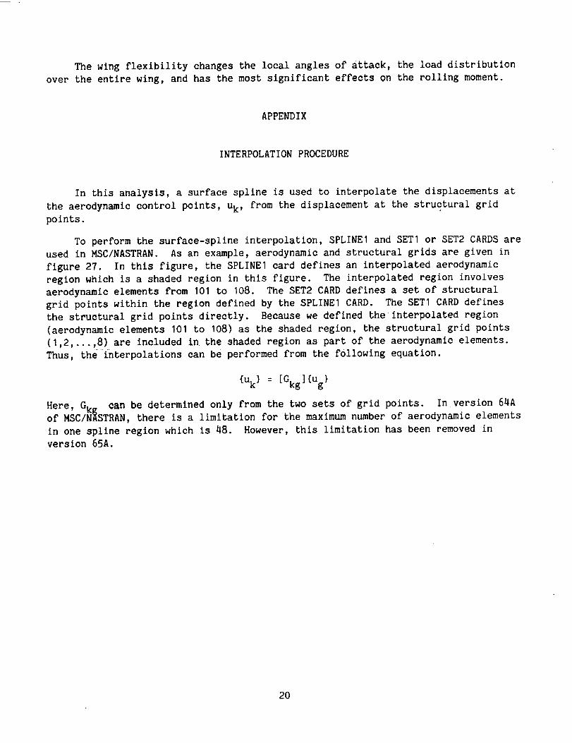
In this analysis, a surface spline is used to interpolate the displacements at

the aerodynamic control points, Uk, from the displacement at the structural grid

points.

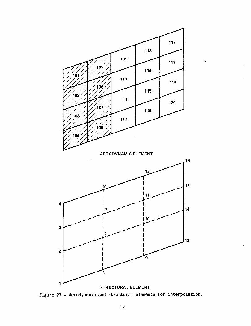
To perform the surface-spline interpolation, SPLINEI and SETI or SET2 CARDS are

used in MSC/NASTRAN. As an example, aerodynamic and structural grids are given in

figure 27. In this figure, the SPLINEI card defines an interpolated aerodynamic

region which is a shaded region in this figure. The interpolated region involves

aerodynamic elements from 101 to 108. The SET2 CARD defines a set of structural

grid points within the region defined by the SPLINEI CARD. The SETI CARD defines

the structural grid points directly. Because we defined the interpolated region

{aerodynamic elements 101 to !08) as the shaded region, the structural grid points

(1,2,...,8) are included in the shaded region as part of the aerodynamic elements.

Thus, the interpolations can be performed from the following equation.

{uk} : [Gkg]{Ug}

Here, Gk_ can be determined only from the two sets of grid points. In version 64Aof MSC/N_STRAN, there is a limitation for the maximum number of aerodynamic elements

in one spline region which is 48. However, this limitation has been removed in

version 65A.

20

REFERENCES

I. Rodden, W. P.; Harder, R. L.; and Bellinger, E. D.: Aeroelastic Addition to

NASTRAN, NASA CR-3094, Mar. 1979.

. Harder, R. L.; MacNeal, R. H.; and Rodden, W. P.: A Design Study for the

Incorporation of Aeroelastic Capability into NASTRAN. NASA CR-111918, Aug.1965.

. Rodden, W. P.; Wilson, C. T.; Herting, D. N.; Bellinger, E. D.; and MacNeal,

R.H.: Static Aeroelastic Addition to MSC/NASTRAN. Paper 15, Proceedings

of the 1984 MSC/NASTRAN User's Conference, Pasadena, CA, Mar. 1984.

. Woodward, F. A.; Tinoco, E. N.; and Larsen, J. W.: Analysis and Design of

Supersonic Wing-Body Combinations, Including Flow Properties in the Near

Field, Part I--Theory and Application. NASA CR-73106, Aug. 1967.

, Woodward, F. A.: Analysis and Design of Wing-Body Combinations at Subsonic and

Supersonic Speeds. J. of Aircraft, vol. 5, no. 6, Nov.-Dec. 1968,

pp. 528-534.

. Albano, E.; and Rodden, W. P.: A Doublet-Lattlce Method for Calculating Lift

Distributions on Oscillating Surfaces in Subsonic Flows. AIAA J., vol. 7,

no. 2, Feb. 1969, pp. 279-285, and vol. 7, no. 11, Nov. 1969, p. 2192.

. Rodden, W. P.; Giesing, J. P.; and Kalman, T. P.: New Developments and Appli-

cations of the Subsonic Doublet-Lattice Method for Nonplanar

Configurations. AGARD-CP-80-71, Paper 4, AGARD Symposium on Unsteady

Aerodynamics for Aeroelastic Analyses of Interfering Surfaces, Tonsberg,

Oslofjorden, Norway, Nov. 1970.

. Rodden, W. P.; Giesing, J. P.; and Kalman, T. P.: Refinement of the Nonplanar

Aspects of the Subsonic Doublet-Lattlce Lifting Surface Method. J.

Aircraft, vol. 9, no. I, Jan. 1972, pp. 69-73.

. Pines, S.; DugundJi, J.; and Neuringer, J.: Aerodynamic Flutter Derivatives

for a Flexible Wing with Supersonic and Subsonic Edges. J. Aero. Sci.,

vol. 22, no. 10, Oct. 1955, pp. 693-700.

10. Ashley, H.; and Zartarian, G.: Piston Theory--A New Aerodynamic Tool for the

Aeroelastician. J. Aero. Sci., vol. 23, no. 12, Dec. 1956, pp. 1109-1118.

11. Harder, R. L.; and Desmarais, R. N.: Interpolation Using Surface Splines. J.

of Aircraft, vol. 9, no. 2, Feb. 1972, pp. 189-191.

21

TABLEI.- COMPARISON OF MAXIMUM DEFLECTION FOR THE DIFFERENT SURFACE

SPLINE REGIONS FOR SWEPT-BACK FLAT-PLATE WING

Number of

surface spline

region

2 (fig. 6(a))

4 (fig. 6(b))

6 (fig. 6(c))

Number of aero-

elements within

one spline region

45

2O - 25

15

Number of structural

grid points within

one spline region

35

15 - 20

15

Maximum

deflection,

in.

116.19

116.43

116.35

TABLE 2.- COMPARISON OF MAXIMUM DEFLECTION FOR THE DIFFERENT SURFACE

SPLINE REGIONS FOR OBLIQUE WING I

Number of

surface spline

region

2 (fig. 10(a))

6 (fig. 10(b))

Number of aero-

elements within

one spline region

45

15

Number of structural

grid points within

one spline region

35

15

Maximum

deflection,

in.

127.18

127.50

TABLE 3.- COMPARISON OF MAXIMUM DEFLECTION

FOR THE DIFFERENT AERO AND STRUCTURAL

ELEMENTS

Number Of

structure

elements

56

88

132

132

Number of

aero-

elements

136

224

144

336

Number of

spl ine

regions

7

8

8

11

Maximum

deflection,

in.

21.02

20.1521.04

19.84

22

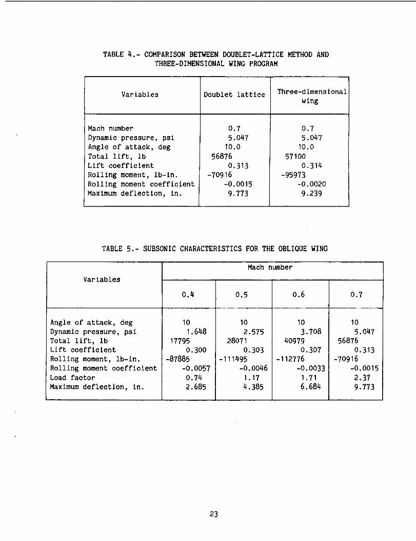
TABLE 4.- COMPARISON BETWEEN DOUBLET-LATTICE METHOD AND

THREE-DIMENSIONAL WING PROGRAM

Variables

Mach number

Dynamic pressure, psi

Angle of attack, deg

Total lift, ib

Lift coefficient

Roiling moment, Ib-in.

Rolling moment coefficient

Maximum deflection, in.

Doublet lattice

0.7

5.O47

10.O

56876

O.313

-70916

-O.OO15

9.773

Three-dimensional

wing

0.7

5.047

10.O

57100

O.314

-95973

-O.0020

9.239

TABLE 5.- SUBSONIC CHARACTERISTICS FOR THE OBLIQUE WING

Variables

Angle of attack, deg

Dynamic pressure, psi

Total lift, ib

Lift coefficient

Rolling moment, Ib-in.

Rolling moment coefficient

Load factor

Maximum deflection, in.

0.4

I0

1.648

17795

0.300-87885

-0.0057

0.74

2.685

Mach number

0.5

IO

2.575

28071

0.303

-111495

-0.0046

1.17

4.385

0.6

IO

3.708

40979

0.307

-112776

-0.0033

1.71

6.684

I

0.7

10

5.047

56876

0.313

-70916

-0.0015

2.37

9.773

23

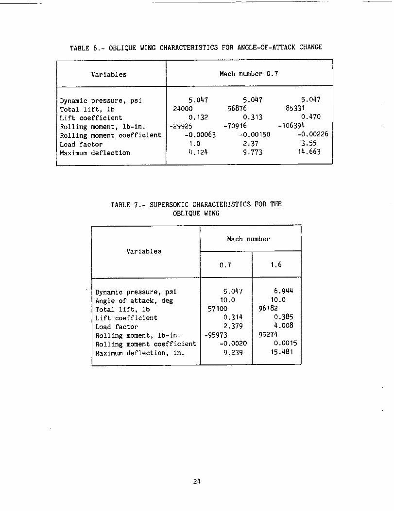
TABLE 6.- OBLIQUE WING CHARACTERISTICS FOR ANGLE-OF-ATTACK CHANGE

Variables

Dynamic pressure, psi

Total lift, Ib

Lift coefficient

Rolling moment, lb-in.

Rolling moment coefficient

Load factor _:

Maximum deflection

Mach number 0.7

5.047 5.047 5.047

24000 56876 85331

0.132 0.313 0.470

-29925 -70916 -106394

-0.00063 -0.00150 -0.00226

1.0 2.37 3.55

4.124 9.773 14.663

TABLE 7.- SUPERSONIC CHARACTERISTICS FOR THE

OBLIQUE WING

Variables

Dynamic pressure, psi

Angle of attack, deg

Total lift, ib

Lift coefficient

Load factor

Rolling moment, lb-in.

Rolling moment coefficient

Maximum deflection, in.

Mach number

5.O47

10.0

1.6

6.944

I0.0

57100

0.314

2.379

-95973

-0.0020

9.239

96182

0.385

4.008

95274

O.0015

15.481

24

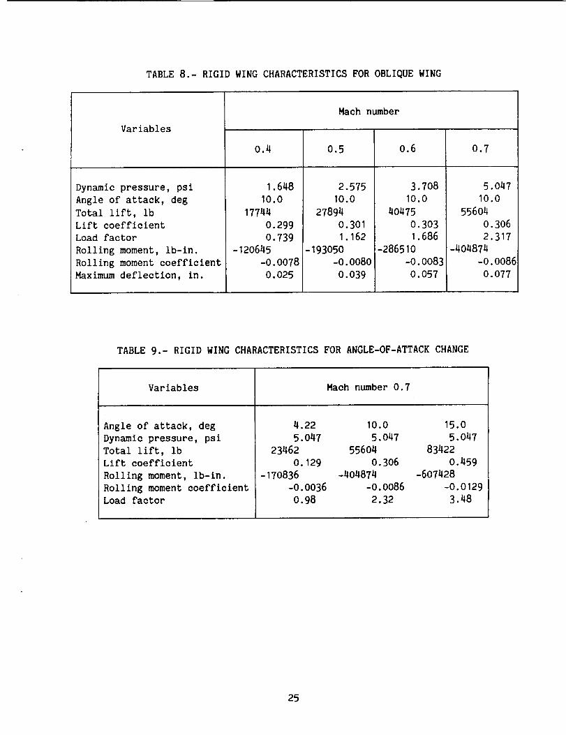
TABLE8.- RIGID WINGCHARACTERISTICSFOROBLIQUEWING

Variables

Machnumber

Dynamicpressure, psiAngle of attack, deg

0.4

1.64810.0

0.5

2.575

10.0

0.6

3.708

IO.O

0.7

5.047

10.0

Total lift, ib

Lift coefficient

Load factor

Rolling moment, ib-ln.

Rolling moment coefficient

Maximum deflection, in.

17744

0.299

0.739

-120645

-0.0078

0.025

278940.3011.162

-193050-0.0080

0.039

40475

0.3031.686

-286510

-0.00830.057

55604

0.306

2.317

-404874

-0.0086

0.077

TABLE 9.- RIGID WING CHARACTERISTICS FOR ANGLE-OF-ATTACK CHANGE

Variables

Angle of attack, deg

Dynamic pressure, psi

Total lift, IbLift coefficient

Rolling moment, ib-in.

Rolling moment coefficient

Load factor

Mach number 0.7

4.22 10.0 15.0

5.047 5.047 5.047

23462 55604 83422

0.129 0.306 0.459

-170836 -404874 -607428

-0.0036 -0.0086 -0.0129

0.98 2.32 3.48

25

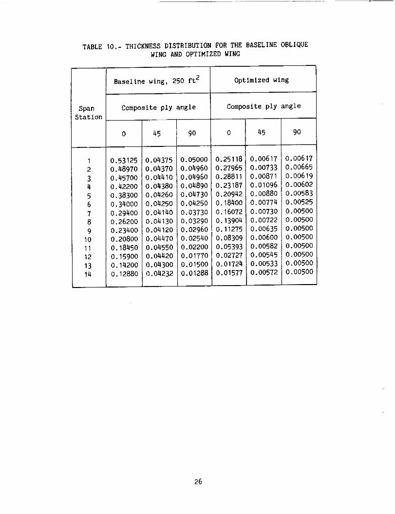
TABLE10.- THICKNESSDISTRIBUTIONFORTHEBASELINEOBLIQUEWINGANDOPTIMIZEDWING

SpanStation

I23456789

I011121314

Baseline wing, 250 ft 2

Composite ply angle

0.531250.489700.457000.422000.383000.340000.29400O.262000.234000.208000.18450

0.15900

0.14200

0.12880

45

0.04375

0.O4370

0.04410

0.04380

0.04260

0.04250

0.04140

0.04130

0.O4120

0.04470

0.04550

0.04420

0.04300

0.04232

9O

0.05000

0.04960

0.04960

0.04890

0.04730

0.0425O

o.03730

0.03290

0.02960

0.02540

0.02200

0.01770

0.01500

0.01288

Optimized wing

Composite ply angle

45

0.00617

0.00733

0.00871

0.01096

0.00880

0.00774

0.007300.00722

0.00635

O.O0600

0.005820.00545

0.005330.00572

0

0.25118

0.27965

0.28811

0.23187

0.20942

0.18400

0.16072

0.13904

0.11275

0.08309

0.053930.02727

0.01724

0.O1577

9O

0.00617

0.00665

0.00619

0.00602

O.OO583

0.00525

0.00500

0.00500

0.00500

0.00500

O.00500

0,00500

0.00500

0.00500

26

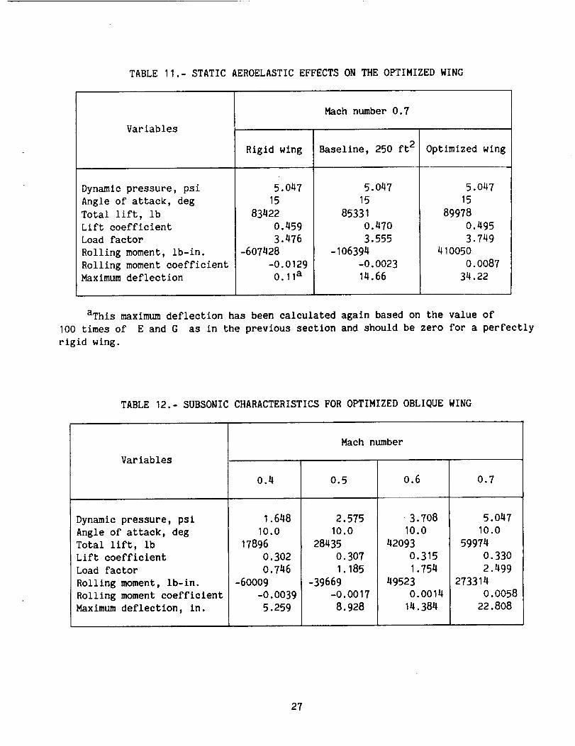
TABLE11.- STATICAEROELASTIC EFFECTS ON THE OPTIMIZED WING

Variables

Dynamic pressure, psi

Angle of attack, deg

Total lift, ib

Lift coefficient

Load factor

Rolling moment, ib-in.

Rolling moment coefficient

Maximum deflection

Rigid wlng

5.047

15

83422

0.459

3.476

-6O7428

-0.0129

0.11a

Mach number 0.7

Baseline, 250 ft2

5.047

15

85331

0.47O

3.555

-106394

-0.0023

14.66

Optimized wing

5.047

15

89978

0.495

3.749

410050

O.OO87

34.22

aThls maximum deflection has been calculated again based on the value of

1OO times of E and G as in the previous section and should be zero for a perfectly

rigid wing.

TABLE 12.- SUBSONIC CHARACTERISTICS FOR OPTIMIZED OBLIQUE WING

Variables

Dynamic pressure, psi

Angle of attack, deg

Total lift, ib

Lift coefficient

Load factor

Rolling moment, Ib-in.

Rolling moment coefficient

Maximum deflection, in.

0.4

1.648

10.0

178960.3020.746

-60009

-O.0039

5.259

Mach number

0.5

2.575

10.0

28435

O.3O7

1.185

-39669-0.0017

8.928

O.6

3.708

10.0

42093

0.315

1.754

49523

0.0014

14.384

0.7

5.04710.0

59974

0.3302.499

2733140.0058

22.808

27

LINE OF DOUBLETS

DOWNWASH

COLLOCATION

POINT

FiEure I.- Aerodynamic elements and location of doublets and collocation

points for doublet-lattice method (ref. 8).

V

a

fj

TUk 1

T/

CENTER OF

PR ESSUR E

Uk 2

11

wj DOWNWASHCENTER

Figure 2.- lll4stration of aerodynamic deErees of freedom.

28

A

//

/

,I f i,/ I i,II /,I I/

X

600"

_-:-y

"'">,7-\ ',\\ '\\

'\_ _°°'_

\

\

Figure 3.- Structural grid for swept-back wing.

# I

I ' /

i _ /

/

vi

i _ _Y

i I" ,, , \\

i \

\ \

Figure 4.- Aerodynamic grid for swept-back wing.

29

-,-,----- TRAILING EDGE

..... LEADING EDGE

Q = 2 psiI--

.z

o=,-lO01-_i , , ... _,'-_-_ /

-300 -200 -100 0 100 200 300

SPAN STATION, in.

-_y

Figure 5.- Displacement in z-direction for swept-back winE.

///

///////

// ///

/_/ ///

//i////////////(a)

\

\\

l_\,R \.\\',,,\\\R

\\\\\ \\

\\

\

_ y

Figure 6(a).- Two-surface spline regions for swept-back wine (surface spline

regions are divided by the thick lines).

3O

///

/ ///

///_/,¢/

(b)

/I/

/

/////////

i

,//

/////////

\

\\

\\ \\\\\\\\\\\\

\

x

=y

\

\\

\'\\\\\\ \,\\\\\\

\1\\',,\

\

b,\\\

\

Figure 6(b).- Four-surface spline regions for swept-back wing.

/A/A�A�i/Z /

Y/

(c)

/iZ

s

ftZ/ /'/]

/ /'/,¢

///o

/ /

/

/A�

///i dl/Zi,/Xi

7ft

f

i

iN/ '\1

11,

/' "4,/' "4,/, N

N \

N\

N_,,jN

\\ _ y

\\,,,\',,\\\",_\\\\,,,1\\\ \ \,,

\\',_

Figure 6(c).- Six-surface spline regions for swept-back wing.

31

T7_

/All

///

///////

/A�

/A// /,4//

f

X

600'"

Figure 7.- Structural grid for oblique-wing I.

32

iiIIiiI/i

IIi

ii/I/i//i

ifl

I//i/i/

li/i/iilll�ill

I

Aiiix,iiii

J"iXi

f

tlliix,,/IX/i/I

i/i/i/i/iliI

_y

FiEure 8.- Aerodynamic Erid for oblique-wln E I.

33

----- TRAILING EDGE

.... LEADING EDGE Q=0.1 psi

.j=,=<:=l •

Lu._¢!,_.*60Q_ I-"

z _ 40

,_ 20 .-_-300 -200 -100 0 100 200 300

SPAN STATION, in.

_Y

Figure 9.- Displacement in z-direction for oblique-wing I.

I

//I/,,_////

///

(a)

//

//////

/

///

X

///////////

i,/"/

,,'/,/i�/

/

///1/I//i///i�/

_- y

Figure 10(a).- Two-surface spline regions for oblique-wing I.

34

///

,,/'/,",,/1

/ /,/ /

/ 7,/ "

I/fl/(b)

Figure 10(b).- Six-surface spline regions for oblique-wlng I.

35

A

Figure 11.- Structural grid for oblique-

wine II (plate model).

X

V

!

!

Figure 12.- Aerodynamic grid for oblique-

wlng II (plate model).

TRAILING EDGE

.... LEADING EDGE Q = 0.5 psiI--

.z

r,-<_ _100O ..11-

- 100 -50 0 50 100SPAN STATION, in.

Figure 13.- Displacement in z-direction for oblique-wing II.

36

Figure 14(a).- Seven-surface spline

regions for oblique-wing II (plate

model), 136 aero elements.

Figure 14(b).- Eleven-surface spline

regions for oblique-winE II (plate

model), 336 aero elements.

37

B_______v---2]_----_ ------_s_-----

r35 i

_3B

_q9 _q _39

z_---y

IX

Figure 15(a).- Structural grid for 250 ft2 baseline oblique wing (upper surface of

left wing).

z y

Figure 15(b).- Structural grid for 250 ft 2 baseline oblique wing (upper surface of

right wing).

38

¥ V

Figure 16.- Aerodynamic grid for 250 ft2 baseline oblique wing.

39

Z

¥_jx

Figure 17(a).- Structural deformation of 250 ft2 baseline oblique wing.

Z

I_y ...... x

Figure 17(b).- Structural deformation of 250 ft2 baseline oblique wing.

4O

2

t_ --,-.--,. 250 ft2 BASELINE OBLIQUE WING

,-- OPTIMIZED WING

,_ •

la)

0 .5 1

(a) 98.5_ aerodynamic semlspan station (left wing).

m

¢z

1

(b)I

.5CHORD

(b) 70.0_ aerodynamic semlspan station (left wing).

Figure 18.- Comparison of pressure distribution between baseline oblique wing

and optimized wing (M = 0.7, a : 10°).

41

2

(I

0 .5 1

(c) 34.0% aerodynamic semlspan station (left wing)

2

1<]

250 ft2 BASELINE OBLIQUE WING

mm OPTIMIZED WING

I

.5CHORD

Figure 18.- Continued. (d) 33.0% aerodynamic semlspan station (right wing).

42

_

1

0

I

\

.5 1

(e) 71.0% aerodynamic semispan station (right wing).

w

o.

<I%

f) A

.5 1CHORD

Figure 18.- Continued. (f) 86.5% aerodynamic semlspan station (right wing).

43

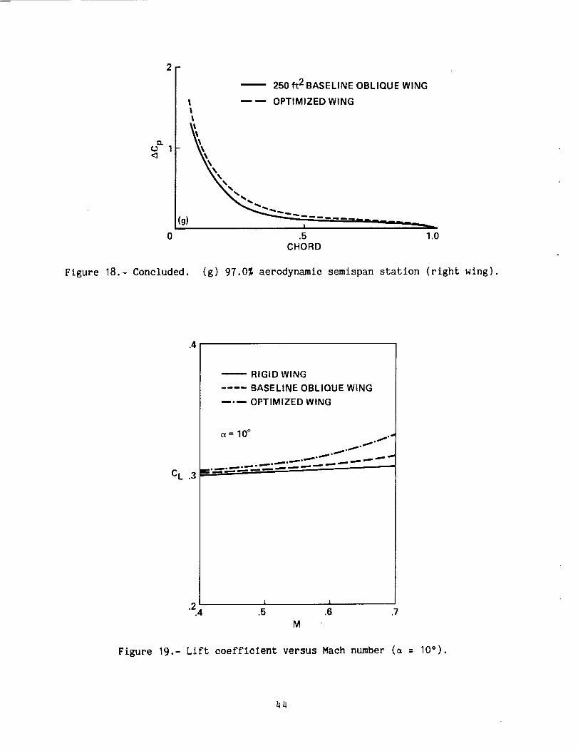
Figure 18° -

j

(J 1-<]

(g)

Concluded.

lll

-- 250 ft 2 BASELINE OBLIQUE WING

---- OPTIMIZED WING

.5

CHORD

(g) 97.0% aerodynamic semispan station

1.0

(right wing).

.4

CL .3

-- RIGID WING

.... BASELINE OBLIQUE WING

--'-- OPTIMIZED WING

= 10° _,.,

1 I

"24 .5 .6 .7

M

Figure 19.- Lift coefficient versus Math number (_ : I0°).

44

.6

.4

C L

,2

-- RIGID WING

.... BASELINE OBLIQUE WING #/'d

--'-- OPTIMIZED WING /'/j

I I

5 10 15

_, deg

Figure 20.- Lift coefficient versus angle

of attack (M = 0.7).

C r

.012

.008

.004

0

-.004

-.008

-.012

•',--'---- RIGID WING

.... BASELINE OBLIQUE WING

---'-- OPTIMIZED WING

.IJ

M = 0.7 1.1. f"

f"f"

f'f"

f"f-

,.f,J"

I i

0 5 10 15

o_,deg

Figure 21.- Rolling-moment coefficient

versus angle of attack (H = 0.7).

45

.010

.OO8

.006

.004

,002

C r 0

-.002

-.004

-.006

-.008

-.010.4

RIGID WING

.... BASELINE OBLIQUE WING

--.-- OPTIMIZED WING ./_

= 10 ° //

././

./f

.//

_._"

L I

.5 .6 .7

M

Figure 22.- Rolling-moment coefficient

versus Haoh number (_ : 10°).

10,

"o

n-

8

6

2

-2

-4

11 --'OPTIMIZED WING

BASELINE OBLIQUE WING, 250 ft 2

M = 0.7

RIGHT WING

RIGHT WING

LEFT WING

LEFTWlNG

I I I 1

0 .2 .4 .6 .8 1.0CHORD

Figure 23.- Bending angle of deformed

wings (74% span station).

Figure

o_cD"o

&er

3m _ OPTIMIZED WING

_BASELINE OBLIQUE WING, 250 ft 2

M = 0.7- RIGHT WING

LEFT WING

RIGHT WING

LEFT WING

l I Z J Tr

0 ,2 .4 .6 .8 1.0

CHORD

24.- Twisting angle of deformed wings (74% span station)•

46

10

-2m

-4

0

m OPTIMIZED WING

BASELINE OBLIQUE WING, 250 ft 2

M = 0.7

RIGHT WING

RIGHT WING

LEFT WING

m

LEFT WING

I i I I

.2 .4 .6 .8 1.0CHORD

Figure 25.-caused by

(74_ span

Local angle-of-attack change

wing twisting and bending

station).

.E

k-

14

12

10

4

.... OPTIMIZED WING" _BASELINE OBLIQUE WING, 250 ft2

M=0.7RIGHT WING

LEFT WING

RIGHT WING

LEFT WING

I 1 I I

0 .2 .4 .6 .8 1.0CHORD

Figure 26.- Vertical displacements of

deformed wings (7q% span station).

4?

117

113

109 / 118

Report Documentation Page

1. Report No.

NASA TM-89423

4. Title and Subtitle

2. Government Accession No, 3. Recipient's Catalog No.

5. Report Date

June 1987

Static Aeroelastie Analysis for GenericConfiguration Aircraft

7. Author(s)

In Lee, Hirokazu Miura, and Mladen K. Chargin

9. Pedorming Organization Name and Address

Ames Research Center

Moffett Field, CA 94035

12. Sponsoring Agency Name and Addre_

National Aeronautics and Space Administration

Washington, DC 20546

6. Performing Organization Code

8. Performing Organization Report No.

A-87091

10. Work Unit No.

533-O6-O1

11, Contract or Grant No.

13. Ty_ of Report and Period Covered

Technical Memorandum

14. Sponsoring Agency Code

15, Supplementary Notes

Point of Contact: H. Miura, Ames Research Center, HIS 237-11

Moffett Field, CA 94035 (415) 694-5888 or FTS 464-5888

16. Abstract

A static aeroelastic analysis capability that can calculate flexible air

loads for generic configuration aircraft was developed. It was made possible by

integrating a finite element structural analysis code (MSC/NASTRAN) and a panelcode of aerodynamic analysis based on linear potential flow theory. The frame-

work already built in _L_C/NASTRAN was used and the aerodynamic influence coef-

ficient matrix is computed externally and inserted in the NASTRAN by means of a

DMAP program. It was shown that deformation and flexible airloads of an obliquewing aircraft can be calculated reliably by this code both in subsonic and

supersonic speeds. Preliminary results indicating importance of flexibility in

calculating air loads for this type of aircraft are presented.

17. Key Words (Suggested by Author(s))

Aeroelastictty, Obliquewing, NASTRAN, Static

aeroelasticlty

19. Security Classif. (of this report)

Unclassified

NASA FORM 1626 OCT 86

Subject Category - 07

20, Security Cla_if. (of this page)

Unclassified

21. No. of pages

5322. Price

A04