fixed rank kriging for very large spatial data setsj. r. statist. soc. b (2008) 70, part 1, pp....

)L[HG�5DQN�.ULJLQJ�IRU�9HU\�/DUJH�6SDWLDO�'DWD�6HWV$XWKRU�V��1RHO�&UHVVLH�DQG�*DUGDU�-RKDQQHVVRQ6RXUFH��-RXUQDO�RI�WKH�5R\DO�6WDWLVWLFDO�6RFLHW\��6HULHV�%��6WDWLVWLFDO�0HWKRGRORJ\��9RO��1R��SS��3XEOLVKHG�E\��:LOH\�IRU�WKH�5R\DO�6WDWLVWLFDO�6RFLHW\6WDEOH�85/��http://www.jstor.org/stable/20203819 .$FFHVVHG��

Your use of the JSTOR archive indicates your acceptance of the Terms & Conditions of Use, available at .http://www.jstor.org/page/info/about/policies/terms.jsp

.JSTOR is a not-for-profit service that helps scholars, researchers, and students discover, use, and build upon a wide range ofcontent in a trusted digital archive. We use information technology and tools to increase productivity and facilitate new formsof scholarship. For more information about JSTOR, please contact [email protected].

.

Wiley and Royal Statistical Society are collaborating with JSTOR to digitize, preserve and extend access toJournal of the Royal Statistical Society. Series B (Statistical Methodology).

http://www.jstor.org

This content downloaded from 128.97.55.209 on Thu, 6 Mar 2014 20:53:38 PMAll use subject to JSTOR Terms and Conditions

http://www.jstor.org/action/showPublisher?publisherCode=black

http://www.jstor.org/action/showPublisher?publisherCode=rss

http://www.jstor.org/stable/20203819?origin=JSTOR-pdf

http://www.jstor.org/page/info/about/policies/terms.jsp


J. R. Statist. Soc. B (2008) 70, Part 1, pp. 209-226

Fixed rank kriging for very large spatial data sets

Noel Cressie

The Ohio State University, Columbus, USA

and Gardar Johannesson

Lawrence Livermore National Laboratory, Livermore, USA

[Received May 2006. Final revision July 2007]

Summary. Spatial statistics for very large spatial data sets is challenging. The size of the data set, n, causes problems in computing optimal spatial predictors such as kriging, since its computa tional cost is of order A73. In addition, a large data set is often defined on a large spatial domain, so the spatial process of interest typically exhibits non-stationary behaviour over that domain. A flexible family of non-stationary covariance functions is defined by using a set of basis functions that is fixed in number, which leads to a spatial prediction method that we call fixed rank kriging. Specifically, fixed rank kriging is kriging within this class of non-stationary covariance functions. It relies on computational simplifications when n is very large, for obtaining the spatial best linear unbiased predictor and its mean-squared prediction error for a hidden spatial process. A

method based on minimizing a weighted Frobenius norm yields best estimators of the covari ance function parameters, which are then substituted into the fixed rank kriging equations. The new methodology is applied to a very large data set of total column ozone data, observed over the entire globe, where n is of the order of hundreds of thousands.

Keywords: Best linear unbiased predictor; Covariance function; Frobenius norm; Geostatistics; Mean-squared prediction error; Non-stationarity; Remote sensing; Spatial prediction; Total column ozone

1. Introduction

Kriging, or spatial best linear unbiased prediction (BLUP), has become very popular in the earth and environmental sciences, where it is sometimes known as optimum interpolation. Matheron

(1962) coined the term 'kriging' in honour of D. G. Krige, a South African mining engineer (Cressie, 1990). With its internal quantification of spatial variability through the covariance function (or variogram), kriging methodology can produce maps of optimal predictions and associated prediction standard errors from incomplete and noisy spatial data (e.g. Cressie (1993), chapter 3). Sometimes a spatial datum is expensive to obtain (e.g. drilling wells for oil reserve

estimation), in which case the sample size n is typically small and kriging can be performed straightforwardly. Recently, with the ubiquity of remote sensing platforms on satellites, data base paradigms have moved from small to massive, often of the order of gigabytes per day. Solving the kriging equations directly involves inversion of an n x n variance-covariance matrix S, where n data may require 0(n3) computations to obtain E_1. Under these circumstances, straightforward kriging of massive data sets is not possible. Our goal in this paper is to develop

methodology that reduces the computational cost of kriging to 0(n).

Address for correspondence: Noel Cressie, Department of Statistics, Ohio State University, 1958 Neil Avenue, Columbus, OH 43210-1247, USA. E-mail: [email protected]

? 2008 Royal Statistical Society 1369-7412/08/70209



210 N. Cressie and G. Johannesson

Even a spatial data set of the order of several thousand can result in computational slow downs. Ad hoc methods of subsetting the data were formalized by the moving window approach of Haas (1995), although it appears that the local covariance functions that are fitted within the

window yield incompatible covariances at larger spatial lags. The variance-covariance matrix X is typically sparse when the covariance function has a finite range, and hence H_1 can be obtained by using sparse matrix techniques. Rue and Tjelmeland (2002) approximated X-1 to be

sparse, approximating it to be the precision matrix of a Gaussian Markov random field wrapped on a torus.

When data sets are large (of the order of tens of thousands) to very large (of the order of hundreds of thousands), straightforward kriging can break down and ad hoc local kri

ging neighbourhoods are typically used (e.g. Cressie (1993), pages 131-134). One avenue of recent research has been to approximate the kriging equations (Nychka et al9 1996, 2002;

Nychka, 2000; Billings et al., 2002 a, b; Furrer et al., 2006; Qui?onero-Candela and Rasmussen, 2005). Suggestions include giving an equivalent representation in terms of orthogonal bases and

truncating the bases, doing covariance tapering, using approximate iterative methods such as

conjugate gradient, implementing sparse approximations using inducing variables or repla cing the data locations with a smaller set of space filling locations. Kammann and Wand

(2003) took up this last idea when fitting a class of spatial models that they called geoadditive models.

Another approach has been to choose classes of covariance functions for which kriging can be done exactly, even though the spatial data sets are large (e.g. Huang et al. (2002), Johan nesson and Cressie (2004a) and Johannesson et al. (2007)). In these papers, a multiresolution

spatial (and spatiotemporal) process was constructed so that (simple) kriging can be computed iteratively and extremely rapidly, with computational complexity linear in the size of the data. In the spatial case, Johannesson and Cressie (2004a) achieved speed-ups of the order of 108 over

directly solving the kriging equations. They could compute optimal spatial predictors and their associated mean-squared prediction errors over the entire globe in about 3 min for n ~ 160000.

One advantage of having a spatial model that allows exact computations is that there is no concern about how close approximate kriging predictors and approximate mean-squared pre diction errors are to the corresponding theoretical values. For exact methods, two important questions are, then, how flexible are the spatial covariance functions that are used for kriging and how are they fitted?

For the multiresolution models that were referred to above, the implied spatial covariances are non-stationary and 'blocky'. In this paper, we use a different approach to achieve orders

of-magnitude speed-ups for optimal spatial prediction, using covariance functions that are very flexible and can be chosen to be smooth or not, as determined by the type of spatial dependence that is exhibited by the spatial data (in contrast with the approach of Tzeng et al. (2005)). We shall show that there is a very rich class of spatial covariances from which kriging of large spatial data sets can be carried out exactly, with a computational cost of 0(n).

In what is to follow, we consider a class of n x n variance-covariance matrices X such that X-1 can be obtained by inverting rxr matrices, where r is fixed; in the application to the total column ozone (TCO) data that is given in Section 4, n was 173405 and r was chosen to be 396. From the derivations that are given in Section 2.3, the number of computations per prediction location in the kriging equations is 0(nr2)9 which increases only linearly with sample size.

Furthermore, suppose that the data set is the result of remote sensing from a satellite that achieves global coverage. Then any spatial dependences in the data will almost certainly be

heterogeneous across the globe. What is new in the methodology that is presented in this paper is that we address both problems (data set size and spatial heterogeneity) directly. The result is



Fixed Rank Kriging 211

a spatial BLUP procedure that we call fixed rank kriging (FRK), which relies on inverting rxr matrices for r fixed and independent of?.

For completeness, we mention another approach to spatial prediction, which is based on smoothing splines. In contrast with kriging, smoothing splines do not rely on a spatial sto chastic process whose covariance function must be modelled, fitted and used for computing the optimal predictor. However, there are knots and a smoothing parameter to be determined and, once again, the size of the spatial data set causes computational difficulties. Hastie (1996) and Johannesson and Cressie (2004b) developed low rank spline smoothers for massive data sets.

To carry out FRK, we must specify the form of the (non-stationary) covariance function; the class that we propose is sufficiently flexible to allow multiple scales of spatial variation to be modelled and yields annxn variance-covariancematrix S whose inverse can be computed straightforwardly. The spatial BLUP that minimizes the mean-squared prediction error involves

S-1 in various matrix computations; we show that FRK has computational cost that is linear in n. The spatial covariance function is fitted to empirical covariances by minimizing a weighted

Frobenius norm. Section 2 presents the kriging methodology and gives the equations that define FRK. In Sec

tion 3, the class of non-stationary covariance functions that are used in FRK is investigated, including how to find the one that best fits the data. Section 4 applies the methodology to TCO

data, where n = 173405; kriging by directly inverting the n x n theoretical variance-covariance matrix of the data is not possible. Section 5 contains discussion and conclusions, which is fol lowed by technical Appendix A.

2. Kriging: optimal linear spatial prediction In this section, we present the notation for kriging, and we equate it with BLUP in a spatial setting. When the spatial data sets are large, exact computation of kriging is generally not possi ble. In the latter part of this section, we show how choice of a particular class of non-stationary spatial covariances allows rapid computation of the kriging predictor (i.e. spatial BLUP) and the kriging standard error (i.e. root-mean-squared prediction error).

2.1. The kriging equations Let {Y(s) : s e D c Ud} be a real-valued spatial process. We are interested in making inference on the 7-process on the basis of data that have measurement error incorporated; consider the process Z(-) of actual and potential observations,

Z(s) = F(s) + e(s), seD, (2.1) where {s(s) : s e D} is a spatial white noise process with mean 0, var{s(s)} = a2 v(s) e (0, oo), s e D, for er2 > 0 and v(-) known. In fact, the process Z(-) is known only at a finite number of spatial locations {si,... ,s?}; define the vector of available data to be

Z^(Z(si),...,Z(sw)y. (2.2) The hidden process Y(>) is assumed to have a linear mean structure,

y(s) = t(s)'a + */(s), seD, (2.3) where t(-) = (t\ ( ),..., tp(-))f represents a vector process of known covariates; the coefficients a =

(a\,..., apY are unknown, and the process v(-) has zero mean, 0 < var{i/(s)} < oo, for all seD, and a generally non-stationary spatial covariance function,




cov{z/(u), i/(v)} =

C(u, v), u, v g D, (2.4)

which for the moment is left unspecified. If we define e, Y and v in an analogous manner to Z, then expressions (2.1)-(2.4) imply a

general linear mixed model,

Z = Ta + 6, 6 = v + ?9 (2.5)

where T is an n x p matrix of covariates (t(si),..., t(sw))'. Observe from model (2.5) that the error term 6 is made up of two independent, zero-mean components, resulting in E(6) =0 and var(?) = X =

(oij)9 where

= {C(Sj,Sj) + (T2v(Sj), i = j9 lJ

\C(si9Sj)9 i?j. On writing C = (C(s?, s;)) and V =

diag{u(si),..., v(sn)}9 it is easily seen that

X = C + a2V. (2.6)

No assumptions of stationarity or isotropy of the covariance function have been made; nor will there be.

Interest is in inference on the 7-process, not the noisy Z-process. For point prediction, we wish to predict the F-process at a location so, so e D9 regardless of whether so is or is not an observation location. Cressie (1993), section 3.4.5, gave a formula for the kriging predictor of F(so) in terms of the covariance function:

y(so) = t(s0)/? + k(so)/(Z-Td), (2.7)

where

d = (T'E"1T)-1T,E"1Z, (2.8)

k(s0)/ = c(s0)/X-1, (2.9)

and c(so) = (C(so, si),..., C(so, $n)Y- The equivalence of equation (2.7) to kriging may not be

immediately apparent, since the traditional derivation of kriging is in terms of the variogram and with no measurement error (i.e. where the ?-process in expression (2.1) is identically 0); see Journel and Huijbregts (1978), chapter V. The kriging standard error is the root-mean-squared prediction error of f(so), [E{Y(so)

? f(so)}2]1/2, which is given by

a*(so) = {C(so,so)-k(s^ (2.10)

As the prediction location so in equations (2.7) and (2.10) varies over D9 a kriging prediction map and a kriging standard error map respectively are generated. (In practice, prediction loca tions are finite in number and typically taken as nodes of a fine resolution grid superimposed onD.)

Inspection of the kriging equations (2.7) and (2.10) shows that X-1 is an essential component and the most obvious place where a computational bottleneck could occur. The inverse of a

generic n x n symmetric positive definite matrix has a computational cost of 0(n3). When n is tens of thousands and above, equations (2.7) and (2.10) will not generally be computable in any reasonable amount of time. In the next subsection, we show how choice of a rich class of covariance functions yields orders-of-magnitude speed-ups for optimal spatial prediction (i.e. kriging).




2.2. Spatial covariance function In general, the covariance function C(u, v) that is defined by expression (2.4) must be positive definite on Ud x Ud. Often C(u,v) is modelled as being stationary, in which case it must be a non-negative-definite function of u - v. In this paper, we take a different approach and instead try to capture the scales of spatial dependence through a set of r (not necessarily orthogonal)

basis functions,

S(u)^(Sl(u),...,Sr(u)Y, ueUd, (2.11)

where r is fixed. Examples of basis functions are given in Section 3.1. For any rxr positive definite matrix K, we model cov{F(u), F(v)} according to

C(n,v) = S(u)'KS(v), u,\eUd, (2.12)

which can be shown to be a non-negative-definite function (Section 3.1) and hence is a valid covariance function (Cressie and Johannesson, 2006). It is possible to add r21(u = v) to expres sion (2.12), although we do not do so in this paper; see Section 5.

It is easy to see that expression (2.12) is a consequence of writing v(s) = S(s)fr], seD, where r] is an r-dimensional vector with var(r/) = K. We call the model for v(-) a spatial random-effects

model. Hence, from expression(2.3), Y(s) = t(s)'? + S(s)'ri, seD, which is a mixed effects linear model that we call a spatial mixed effects model.

2.3. Fixed rank kriging From expression (2.12), we can write the nxn theoretical variance-covariance matrix of Y (or v) as C = SKS', and hence

E = SKS/ + a2V, (2.13) where the unknown parameters are K, a positive definite rxr matrix, and a2 > 0. Both S, the nxr matrix whose (/,/) element is S/(s?), and V, a diagonal matrix with entries given by the

measurement error variances, are assumed known. Further,

cov{F(so), Z} = c(so)' = S(so)'KS', (2.14) i.e., on the basis of the model (2.1), (2.3) and (2.12), we can find expressions for all the compo

nents that are needed in the kriging equations (2.7) and (2.10). There remains the problem of n being very large to massive but, as we shall now show, the

choice of covariance function (2.12) allows alternative ways of computing the kriging equations involving inversion of only rxr matrices. Recall from equation (2.13) that T, ? SKS' + a2\,

where V is diagonal. Then

E-^^-^-^?I + ??j-^-^K^-^-^S)7}-1^-^-1/2. (2.15)

Now, it is easy to see that, for any nxr matrix P,

I + PKP' = I + (I + PKP)PK(I + P PK)1^.

Multiplying by (I + PKP V1 yields

(i+PKP)1 =i-pqt1 +pp)1p/, which is a result that is covered by the Sherman-Morrison-Woodbury formulae (see Henderson and Searle (1981)). This is then used in equation (2.15) to give the computational simplification




X-^^V)-1-^^)-^^-^^^^)-^}-1^^^)"1. (2.16)

Note that the formula (2.16) for X"1 involves inverting the^jced rank rxr positive definite matrices and the n x n diagonal matrix V. Finally then, the kriging predictor (spatial BLUP) (2.7) is

F(s0) = t(s0)'d + S(so)/KS/X"1 (Z -

Td), (2.17)

where d = (T/E~1T)~1T/E~1Z and X-1 is given by equation (2.16). The kriging standard error

(2.10) is

ak(s0) = {S(so)'KS(s0)

- S(s0)/KS/X-1SKS(s0) + (t(s0)

- T/X-1SKS(so))/(T/X-1T)"1 (t(s0)

-rx^SKSiso))}172, (2.18) where X-1 is again given by equation (2.16). FRK is the name that we gave to the methodol

ogy that leads to equations (2.16)?(2.18) (Cressie and Johannesson, 2006). As the prediction location so in equations (2.17) and (2.18) varies over D9 a kriging prediction map and a kriging standard error map respectively are generated.

Inspection of equations (2.16)?(2.18) reveals that, for a fixed number of regressors p and a fixed rank r of K in the covariance model that is defined by expression (2.12), the computa tional burden of FRK is only linear in n. To see this (and without loss of generality assume here that cr2V = I), computations that are associated with equations (2.17) and (2.18) involve

computations of S'X^S, SrX_1a and X-1a, for given vectors a of length n. To carry out these

computations, A = S'S and B = (K_1 + S'S)-1 are computed initially, at a maximum computa

tional cost of 0(nr2) (we assume that n >r). Then, from equation (2.16), S/X~1S = A- ABA, and ABA requires 0(r3) computations. The quantities S'X^a and X-1 a have a computational cost that never exceeds 0(nr2). Finally, equation (2.17) has 0(r) computations, and equation (2.18) has 0(r2) computations (assuming that p<Cr) for a fixed so. Hence, the overall com

putational cost is 0(nr2). As confirmed by the timings that are given in Section 4, the FRK

methodology makes it feasible to construct maps of kriging predictors and kriging standard errors that are based on very large spatial data sets.

The relationships between kriging methodology and smoothing methodology are quite well established by now (e.g. Cressie (1993), section 5.9, and Nychka (2000)). Indeed, FRK, which

depends on the covariance model (2.12), was motivated by a fixed rank smoothing technique that evolved from regularization and ridge regression (Johannesson and Cressie, 2004b). The

novelty of our methodology is the combination of & fixed rank positive definite matrix K (the parameter to be estimated) and basis functions {?/( )} (to be specified) that yield a very flexible

spatial covariance function (2.12), followed by computationally efficient (linear in the number of data) kriging predictors and kriging standard errors for large spatial data sets.

In the next section, we consider inter alia estimation of K and the measurement error variance o2 in detail.

3. The class of covariance functions

Recall, from expression (2.12), the class of covariance functions that we are considering in this

paper:

C(u,v) = S(u)'KS(v), u,vgIRj,

where K is an r x r positive definite matrix and S(-) is an r x 1 vector made up of basis functions

S\ ( )> , Sr(-), where r is fixed. This is similar to the form that was given by Stroud et al. (2001),




although they used it to motivate a spatiotemporal model and did not have in mind inverting ? for kriging. In the subsections that follow, we give some properties of this class of covariance functions. We also show how, in a classical geostatistical sense, the data are used twice (e.g. Cressie (1989)). Not only are they present (linearly) in the kriging predictor (2.7); they are also used (non-linearly) to obtain an estimator of the spatial dependence parameters K and a2.

3.1. Some basic properties Most importantly, the function C(u, v) is non-negative definite, the proof of which is straight forward: for any locations {s? : / = 1,..., m} in Ud, any real {b? : / = 1,..., m}, and any integer

m, then (using obvious notation), m m

Z ? bibjC(Si,Sj) = bm(SmKS^)bm = (S>m)/K(S>m) ^0, i"=l 7=1

since K is positive definite. A related model to expression (2.12), but different from C(-, ) given above, is a consequence of

the Karhunen-Lo?ve expansion (e.g. Adler (1981), section 3.3). Define the covariance function 00

Ci(u,v)ee?A,<Mu)<Mv), (3.1) 1=1

where {?/} and {4>i(-)} are non-negative eigenvalues and orthonormal eigenfunctions respec tively, which are obtained from the integral equation

/ Ci(u,v)^(v)dv = A^>(u).

On truncating at the kth term of function (3.1), we obtain a different covariance function,

C2(u, v) = ? A/ 0/(u) 0/(v) = 0(u)'A 0(v), i=\

where A is a k x k diagonal matrix of non-negative entries. Without loss of generality, assume that the truncation keeps only terms with positive eigenvalues; then clearly the truncated Kar hunen-Lo?ve expansion is a special case of expression (2.12). Conversely, if we write K in its spectral form, K = PAP', we see that C(u, v) = (P' S(u))'A(P' S(v)), which looks like a truncated

Karhunen-Lo?ve expansion but with non-orthogonal functions {</>/( )}. To sum up, model

(2.12) involves a fixed rank variance-covariance matrix K (in general, not the identity matrix I) to be estimated and a finite set of basis functions (in general, not orthogonal) to be chosen.

3.2. Basis functions Because we make no requirement of orthogonality of basis functions, the choice of S\(-),..., Sr(-) is unrestricted and may include inter alia the smoothing spline basis functions (e.g. Wahba

(1990)), the wavelet basis functions (e.g. Vidakovic (1999)) and the radial basis functions (e.g. Hast?ela/. (2001), pages 186-187). Whereas K is estimated from the data, S(-) = (Sx(-),..., Sn(-))f is not. Nychka (2000) and Nychka et al (2002) have brought together various choices of basis functions, where they assumed either r = n (i.e. r is equal to the sample size and hence not fixed or if r is fixed then K is diagonal). The ability of the class (2.12) to approximate other covariance functions that are used in geostatistics, such as an isotropic exponential model, is convincingly demonstrated in Nychka et al. (2002). In fact, in Section 4 we shall be doing kriging on the globe, where we choose the basis functions to be multiresolution local bisquare functions.




Our main recommendation regarding the choice of basis functions is that they be multi resolutional. This enables the covariance function model (2.12) to capture multiple scales of variation. In Section 2.2, it is seen that model (2.12) can equivalently be thought of as a spatial random-effects model, S(-)'r?, where the random effects rj have dependence structure given by

K. Hence, multiresolutional components of S(-) allow many spatial scales of variation to be

captured. Indeed, a large spatial scale that is missed by the mean function tO'c* in expression (2.3) can potentially be recovered by some of the spatial random-effects components of S(-)frj.

Obvious classes of multiresolutional functions are different types of wavelets; equally, the class of local bisquare functions that are used in Section 4 is multiresolutional (but not orthog onal). In fact, in an analysis of satellite data on aerosols, Shi and Cressie (2007) choose the

(non-orthogonal) PT-wavelets as components of both the vector of mean functions t() and the covariance basis functions S(-). In this case, the problem reduces to one of model choice

regarding which wavelets are used in t(-) and which are used in S(-), a solution to which is given by Shi and Cressie (2007). The more difficult problem of choosing which class of basis functions to use, from among several, is currently under investigation. Should we wish to compare two FRK maps to detect unusual differences, we recommend that the components of t(-) and S(-) be the same for the two maps.

From a computational point of view, it is beneficial to use a class of basis functions for which it is quick to evaluate S'V_1S and S'a for any a. Although we have seen in Section 2.3 that such

computations are in general 0(nr2)9 by using the bisquare class in Section 4 or wavelet classes and

sparse matrix libraries, the computational cost can be reduced in practice to 0(kr2) where k < n.

3.3. Fitting the covariance function The strategy that we adopt to fit the spatial covariance function is consistent with the geostatis tical approach that is found in classical expositions, like that of Matheron (1963) and Journel and Huijbregts (1978). In that approach, an empirical estimator is first obtained for X, which is based on the method of moments. The resulting estimator X is noisy and may not be positive

definite. However, on the basis of a parametric class {X(0) : 0 e 6}, where each member of the class is positive definite, one chooses a 0 e 6 such that X(0) is 'closest' to X. Finally, the

resulting X(0) is substituted into the kriging equations (2.17) and (2.18). In what is to follow, we see that the spatial dependence parameters 0 are made up of the

rxr positive definite matrix K and a variance component a2 e (0, oo). Estimates K and a2 are obtained from minimizing a Frobenius norm between an empirical variance-covariance matrix and a theoretical variance-covariance matrix.

First, we define an empirical estimator of the variances and covariances, for which we need detrended data. In the absence of initial knowledge of the spatial dependence and for compu tational speed, we use the ordinary least squares estimator of a,

? = (T,TT1T/Z, (3.2)

from which we define the detail residuals,

D(Si) = Z(Sf) -

t(s/)'?, / = 1,..., n. (3.3)

As in classical geostatistics, we 'bin' the data for computation of the method-of-moments estimator of the spatial dependence. The number of bins, M, is meant to be fixed but larger than r, the number of basis functions. Hence, for estimation and fitting of covariances, once the data have been binned the computational complexity does not depend on n. Suppose that

{uj : j = 1,..., M}9 where r < M < n9 is a set of locations, or bin centres, offering good coverage of D. Around thejth bin centre u;, define a neighbourhood N(uj) and 0-1 weights,



w


\\, iisieN(\Xj), 34) Jl \0, otherwise,

v '

i = l,...,n, j=l,...,M. Denote y/j =

(wj\,...,Wjn)' and define

Z7^w;.(Z-T?)/w;i?, (3.5)

where \n is the n x 1 vector of Is, to be the average detrended data that are associated with bin

centreuy, j=l,...,M. In approximation (A.4) in Appendix A, we show how Em = var(Zi,..., Zu) can be approx

imated by Sm(K, g2) == SKS' + a2Y, where S and V are easily computable binned versions of

S and V; as in classical geostatistics, the approximation is caused by small biases due to the

binning. Also, in expression (A.2) in Appendix A, we give an empirical positive definite estimate

?m that isbased on the detail residuals (3.3). We then choose K positive definite and a2 e (0, co) such that ?m(K, &2) is as 'close' to Em as possible.

There are various matrix norms between two matrices A and B of the same order. The one that we shall use is the Frobenius norm,

||A-B||2^tr{(A-B)/(A-B)} = ?(A^-^)2, (3.6)

which has also been used by Hastie (1996) in deriving pseudosplines, and by Donoho et al

(1998) in estimating co variances. We shall ultimately use a weighted Frobenius norm, in the same spirit as weighted least squares estimation of the variogram (Cressie, 1985), but for the

moment we consider the unweighted version (3.6). _ When a2 = 0, Em(K,0) = SKS'. Using the Frobenius norm, the K that minimizes ||?m

-

Em(K, 0) || is given by (see Appendix A) K = RlQ?MQ(R-ly, (3.7)

and the corresponding fitted variance-cov?riance matrix is ?m(K,0) = QQ/?mQQ'? where S = QR is the (^-^-decomposition of S (i.e. Q is an M x r orthonormal matrix and R is a non

singular rxr upper triangular matrix). The computational cost of the ^-^-decomposition is

0(r3). Since Em is positive definite, so also is K. When a2 g (0, oo),

||?M-?M(K,a2)|| = ||?M-a2V-SKS,||,

resulting in the optimal parameter estimate (in terms of a given a2)

K = R-lQ'(?M-a2Y)Q(R-ly; (3.8)

the corresponding fitted variance-covariance matrix is ?m(K, a2) given by

?M(K, a2) = QQ'(?m -

cr2\)QQf + a2Y = QQEmQQ7 + a2(\ - QQVQQ). (3.9)

Thus, <t2 can be obtained by minimizing with respect to a2 e (0, oo):

|| ?M - ?m(K, a2) ||2 = ?{(EM -

P(tM))jk - o-2(V - P(V)),*}2, M

where P(A) = QC^AQQ' for any MxM matrix A. The computational cost of this is 0(M3).

Note that this is just a simple linear regression with slope a2 and zero intercept. Hence the minimization, which is constrained so that equation (3.8) is positive definite and a2 e (0, oo), is easily carried out. The result is




K = R-lQ\tM-?2\)Q(R-ly. (3.10)

For r<M9 the computational cost of parameter estimation is 0(M3), which implies that a good choice of M is one that is independent of n and hence does not dominate the computational cost, 0(nr2)9 of kriging; see Section 4 for comparisons of timings.

Finally, with spatial covariance parameter estimates K and o29 we can implement kriging; the estimates are substituted into equations (2.16)?(2.18). The resulting FRK involves matrix inver sions of fixed rank rxr matrices and annxn diagonal matrix, thus achieving a computational complexity that is linear in the number of data.

More weight should be given to bins that are less variable or have more data. Consider the

weighted Frobenius norm,

\\?M-i:M(K9o2)\\2a = Y.aM&M) (3.11)

where a\,..., a m are known positive weights. Equivalently,

IIXm-Xm^^II^II?^Xm?^-?^Xm^^?1/2!^ where A =

diag(?*i,..., um), i.e. the weighted version of the Frobenius norm involves just scaling the rows and columns of Xm and Xm(K, o2) by {a3 : j = 1,..., M}9 and hence it is computa tionally no more onerous than the unweighted version. From expression (A. 5) in Appendix A,

we motivate statistically the choice to be

ajcx(Wjln)^2/VD(uj)9 j=\9...9M9

which is a data-based weight where Vd(u/) is the empirical variance in theyth bin, given by expression (A.l) in Appendix A.

In summary, the problem of estimation of K and o2 is based on minimizing a weighted Frobe nius norm. This is a weighted least squares criterion that is directly analogous to the approach that was given by Cressie (1985) for variogram estimation. It is moment based, not likelihood based. Under assumptions of Gaussianity, the likelihood of K and o2 depends on X-1 and |X|. From the Sherman-Morrison-Woodbury formula (2.16), we obtain X-1. A like formula yields

|X| = |cr2V||K||K-1 +S'(cr2V)_1S|, which involves determinants of r x r matrices, i.e. compu tation of the likelihood of K and o2 is feasible; however, its maximization is problematic unless

K is further parameterized (Stein, 2008). Fuentes (2007) gives approximate likelihoods for large spatial data sets under assumptions of Gaussianity and covariance stationarity.

4. Fixed rank kriging of total column ozone satellite data

The problem of measuring TCO has been of interest to scientists for decades. Ozone depletion results in an increased transmission of ultraviolet radiation (290-400 nm wavelength) through the atmosphere. This is mostly deleterious because of damage to DNA and cellular proteins that are involved in biochemical processes, affecting growth and reproduction.

Relatively few measurements of TCO were taken in the first quarter of the 20th century. Sub

sequently, with the invention of the Dobson spectrophotometer, researchers gained the ability to measure efficiently and accurately TCO abundance (London, 1985). A system of ground based stations has provided important TCO measurements for the past 40 years; however, the

ground-based stations are relatively few in number and provide poor geographic coverage of the earth. The advent of polar orbiting satellites has dramatically enhanced the spatial coverage of measurements of TCO.




The Nimbus-7 polar orbiting satellite was launched on October 24th, 1978, with the total ozone mapping spectrometer instrument aboard. The instrument scanned in steps of 3? to an extreme of 51? on each side of nadir, in a direction that was perpendicular to the orbital plane (McPeters et al, 1996). Each scan took roughly 8 s to complete, including 1 s for retrace (Madrid, 1978). The altitude of the satellite and scanning pattern of the total ozone mapping spectrom

eter instrument are such that consecutive orbits overlap, with the area of overlap depending on the latitude of the measurement. The satellite was sun synchronous, staying on the plane between the Earth and the Sun. Successive orbits moved westwards because of the rotation of the Earth, and hence the Nimbus-7 satellite covered the entire globe in a 24-h period. The instrument is a passive sensor and relies on backscattered light, which means that there are very few observations in winter near the poles.

On receiving satellite data, NASA calibrates them ('level 1') and preprocesses them to yield spatially and temporally irregular TCO measurements ('level 2'). The level 2 data are subse

quently processed to yield a daily, spatially regular data product that is released widely to the scientific community ('level 3'). The level 3 data product for TCO used Io latitude by 1.25? lon

gitude ( 1 ? x 1.25?) pixels (McPeters et al ( 1996), page 44). Level 2 TCO data were obtained from the Ozone Processing Team of NASA-Goddard, Distributed Active Archive Center, and were stored in hierarchical data format as developed by the National Center for Supercomputing

Applications at the University of Illinois. In what is to follow, we use kriging, in particular FRK, to predict TCO data at the centre of

the Io x 1.25? grid, on a daily basis, i.e. the prediction is at level 2 spatial support on the regular level 3 grid. The example is meant as an illustration of the ability of FRK to handle very large

data sets; Shi and Cressie (2007) use FRK to produce a level 3 data product for aerosol optimal depth based on measurements from the multiangle imaging spectroradiometer instrument on the Terra satellite.

In this section, we use the 173405 level 2 TCO data that are available for October 1st, 1988; see Fig. 1. We implement FRK based on the kriging equations (2.16)-(2.18); some of the practical aspects of this optimal spatial prediction are now discussed.

Fig. 1. Level 2 TCO data on October 1st, 1988, in Dobson units




Fig. 2. Centre points of three resolutions of a discrete global grid

The basis functions that we choose in the spatial covariance model (2.12) are made up of three scales of variation. Each scale has 32,92 and 272 functions associated with them, corresponding to the centre points of a discrete global grid (Sahr, 2001); see Fig. 2. The generic basis function in our spatial covariance model is the local bisquare function:

5?A(u) = /{l-(ll?-Vy(/)IIA/)2}2, ||u-v,(/)Kr/, A) \0, otherwise,

where v/(/) is one of the centre points of the /th resolution, / = 1,2,3, and

n = 1.5(shortest great arc distance between centre points of the /th resolution).

For example, for /= 1, the shortest distance is 4165 km, and hence r/ = 6747.5; the distances between centre points from resolution 2 and 3 are 1610 km and 1435 km respectively. Note that there are a total of r = 32 + 92 + 272 = 396 basis functions.

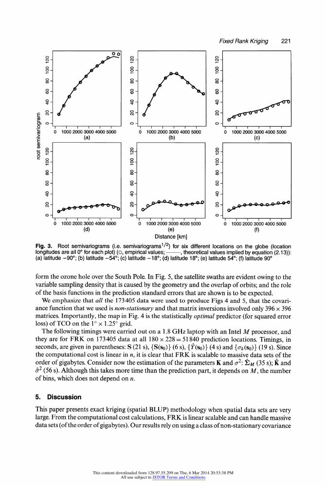
The data were binned to carry out parameter estimation; see Section 3.3. We chose M = 812 and {ui,... ,11812} to be the centre points of resolution 4 of the discrete global grid that was referred to above. After computing the method-of-moments estimator ?^, K and o2 were esti

mated assuming a constant mean, E{Y(s)} = a (i.e. t(s) =

1), and V = I. Fig. 3 shows excellent fits of the theoretical semivariograms to the empirical semivariograms, at six locations on the

globe. At a given location on the globe, the empirical semivariogram, as a function of spatial lag, was calculated from all data within a radius of 3000 km of the location. The same averages were taken of the (non-stationary) theoretical variogram values that are implied by the covariance function (2.12). The result is an averaged theoretical semivariogram that is now a function of

spatial lag, and it is this that is compared with the empirical semivariogram in Fig. 3. This is a diagnostic summary that is easier to assess than empirical and fitted covariance functions at individual locations on the globe.

On substituting the estimates of K and o2 into equations (2.7) and (2.10), we obtain the FRK predictor and the FRK standard error respectively. On the regular Io x 1.25? grid, this

yields Fig. 4 and Fig. 5 respectively. Fig. 4 shows a smooth map of TCO with the characteristic

large TCO values around the ?55? latitudinal zone, from which they decrease precipitously to




o. E w CO

?) o o "i? CO

>

o o

1-1-1-1-1-1? 0 1000 2000 3000 4000 5000

(a)

n-1-1-1-1-r 0 1000 2000 3000 4000 5000

(b)

i-1-1-1-1-r 0 1000 2000 3000 4000 5000

(C)

n-1-1-1-r 0 1000 2000 3000 4000 5000

(d)

n-1-r 0 1000 2000 3000 4000 5000

(e) Distance [km]

i-1-1-1-1-r 0 1000 2000 3000 4000 5000

(f)

Fig. 3. Root semivariograms (i.e. semivariograms1/2) for six different locations on the globe (location longitudes are all 0? for each plot) (o, empirical values;-, theoretical values implied by equation (2.13)): (a) latitude -90?; (b) latitude -54?; (c) latitude -18?; (d) latitude 18?; (e) latitude 54?; (f) latitude 90?

form the ozone hole over the South Pole. In Fig. 5, the satellite swaths are evident owing to the variable sampling density that is caused by the geometry and the overlap of orbits; and the role of the basis functions in the prediction standard errors that are shown is to be expected.

We emphasize that all the 173405 data were used to produce Figs 4 and 5, that the covari ance function that we used is non-stationary and that matrix inversions involved only 396 x 396

matrices. Importantly, the map in Fig. 4 is the statistically optimal predictor (for squared error

loss) of TCO on the Io x 1.25? grid. The following timings were carried out on a 1.8 GHz laptop with an Intel M processor, and

they are for FRK on 173405 data at all 180 x 228 = 51840 prediction locations. Timings, in seconds, are given in parentheses: S (21 s), {S(so)} (6 s), {F(so)} (4 s) and {cr?(so)} (19 s). Since the computational cost is linear in n, it is clear that FRK is scalable to massive data sets of the order of gigabytes. Consider now the estimation of the parameters K and o2\ ?m (35 s); K and <72 (56 s). Although this takes more time than the prediction part, it depends on M, the number

of bins, which does not depend on n.

5. Discussion

This paper presents exact kriging (spatial BLUP) methodology when spatial data sets are very large. From the computational cost calculations, FRK is linear scalable and can handle massive

data sets (of the order of gigabytes). Our results rely on using a class of non-stationary covariance




Fig. 4. FRK prediction of TCO for October 1 st, 1988, in Dobson units

Fig. 5. FRK Standard errors of the TCO predictions that are shown in Fig. 4, in Dobson units

functions that arise from a spatial random-effects model. Recall from equation (2.12) that

C(u, v) = S(u)'KS(v), u, v Rd9

where S() = (S\ ( ),..., Sr(-))' is a vector of basis functions. The rxr positive definite matrix K is a spatial dependence parameter, which we estimate in a classical geostatistical manner by using weighted least squares; maximum likelihood estimation of K is a topic of future research. A Bayesian approach, which is under development, puts a prior (e.g. a Wishart distribution) on K. The Bayesian model specification might then be completed by assuming, for example, that

Y(-) is a Gaussian process that is independent of the Gaussian white noise process ?( ), and that the prior on o2 is a gamma distribution.




A Bayesian analysis would also allow optimal spatial prediction in non-linear geostatistical models of the sort that were considered by Diggle et al (1998). Although such models may be

computationally heavy for large spatial data sets, owing to Markov chain Monte Carlo com

putations that are used in the analysis, there is still an opportunity to achieve computational speed-ups by using the spatial model (2.12). As evidence of this, Hrafnkelsson and Cressie (2003) compared a standard geostatistical covariance model with a model where inverse covariance

matrices were modelled directly, and they reported that the latter led to a factor of more than 5 in increased computational efficiency.

Microscale variation in the (hidden) 7-process could be modelled by including another diag onal matrix in equation (2.6). When both diagonal matrices are proportional to each other, the

measurement error parameter a2 and the microscale parameter r2 are not individually identi

fiable, although their sum r2 + a2 is. The sum is often referred to as the 'nugget effect' in the

geostatistical literature. In this paper we have assumed that F(-) is smooth (i.e. r2 = 0) and the rest of the variability is due to measurement error.

The non-stationary covariance functions that are given by expression (2.12) have remark able change-of-support properties. Let B c Ud and define Y(B) =

JB Y(s) ds/\B\, where |2?| is the ?/-dimensional volume of B. Then

cov{y(fi1),y(B2)} = S(5i),KS(B2), ?i,?2CRd, where S(B) = (Si(B),..., Sr(B))' and Si(B) =

?B S/(s) ds/|?|, for B c Ud. Thus, no matter the

support of the data and the predictor, the kriging equations take the same form as equations (2.16)?(2.18). In practice, the basis functions would be integrated offline.

Finally, there is a natural generalization from the spatial random-effects model, u(s) = S(s)fr?9 which is given in Section 3.2, to a spatiotemporal random-effects model u(s, t) = S(s)' r](t), where

{77(t) : t = 0,1,2,...} is an r-dimensional time series with mean 0 and coy{rj(t\ ), r?fe)}=K(t\, tj), t\Ji = 0,1,2,.... Spatiotemporal kriging and spatiotemporal Kaiman filtering that are based on this model, and a mixed model version involving trend, are currently under investigation.

Acknowledgements

We thank the Associate Editor and the referees for their helpful comments. This research was

supported by the Office of Naval Research under grant N00014-05-1-0133. Partial support was also received from the US National Science Foundation under award DMS-0706997.

Appendix A In Section 3.3, it was assumed that a positive definite estimate EM was available. We now define such an

estimate. For any two bin centres u, and u*, define the empirical covariances that are based on the detail residuals that are defined by expression (3.3):

n n

CD(Uj,uk)= ? ? wjhwki2 D(sh)D(si2)/(Wjln)(Wkln) n=i/2=i

= D(uj)D(uk), j,k=l,...,M,

where, for j=l,...,M,

D(uj) = f2wjiD(si)/Wjln.

Further, for any bin centre u7, define the empirical variance,




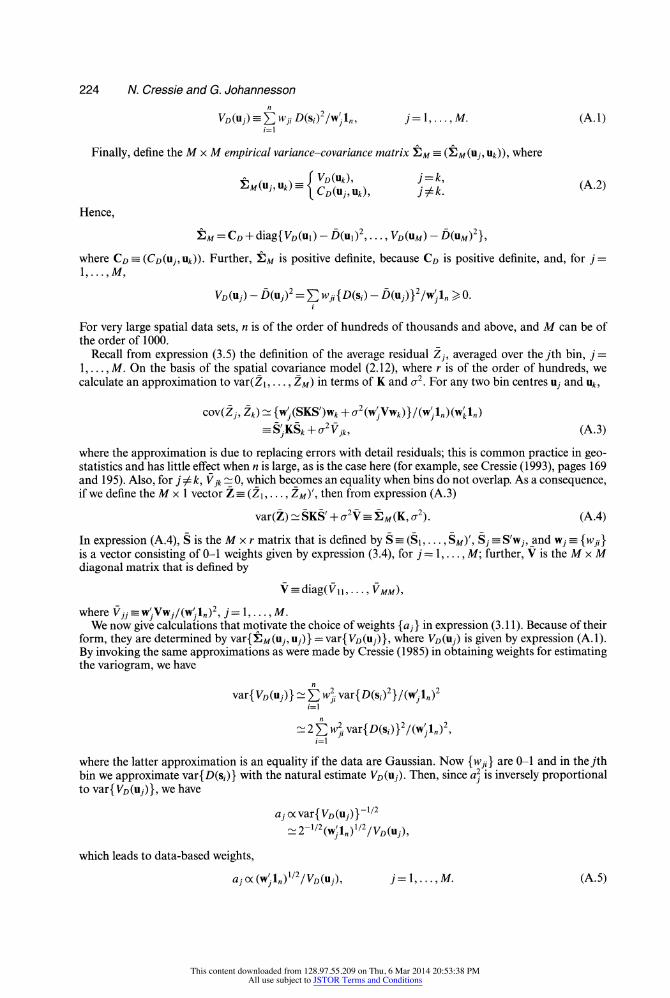
VD(u7)^?w;7D(Sl)2/w;i?, 7 = 1,..., M. (A.l)

Finally, define the M x M empirical variance-covariance matrix XM = (XM(u;, uk))9 where

*M(uJ>Uk) = \CD(uJ9uk)9 j?k. (A-2)

Hence,

?? = CD + diag{ VD(n,) - D(u,)\..., VD(uM) - D(uM)2},

where C?> = (C?(u,-,Ut)). Further, ?M is positive definite, because CD is positive definite, and, for j = \,...,M,

VD(uj) -

D(uj)2 = ? wfi{D(?,) -

D(u,)}2/w;i? > 0. I

For very large spatial data sets, n is of the order of hundreds of thousands and above, and M can be of

the order of 1000. Recall from expression (3.5) the definition of the average residual Zj9 averaged over theyth bin, j =

1,..., M. On the basis of the spatial covariance model (2.12), where r is of the order of hundreds, we calculate an approximation to var(Zi,..., ZM) in terms of K and a2. For any two bin centres u; and uk9

cov(Z7, Zk) ~ {w;.(SKS>* + a2(w^w*)}/(W;in)Kl J

^s;.KS,+?T2y^, (A.3)

where the approximation is due to replacing errors with detail residuals; this is common practice in geo statistics and has little effect when n is large, as is the case here (for example, see Cressie (1993), pages 169 and 195). Also, for j ̂ k, Vjk ̂ 0, which becomes an equality when bins do not overlap. As a consequence, if we define the M x 1 vector Z =

(Zi,..., ZM)', then from expression (A.3)

var (Z) ~ SKS' + a2 V = ?M (K, a2). (A.4)

In expression (A.4), S is the M x r matrix that is defined by S = (Si,..., SM)', S; = S'w;, and w, = {wp} is a vector consisting of 0-1 weights given by expression (3.4), for j = 1,..., M ; further, V is the M x M diagonal matrix that is defined by

Vsdiag(Vn,..., Vmm),

where Vjj =

w;.Vw,/(w;i?)2, j = 1,..., M. We now give calculations that motivate the choice of weights {aj} in expression (3.11). Because of their

form, they are determined by var{?M(u/, u7)} = var{VD(u7)}, where VD(Uj) is given by expression (A.l). By invoking the same approximations as were made by Cressie (1985) in obtaining weights for estimating the variogram, we have

var{ VD(u7-)} ~

? w2 var{D(s;)2}/(w;in)2

~2?viAvar{D(s?)}7(S-l?)2> i=\

where the latter approximation is an equality if the data are Gaussian. Now {wp} are 0-1 and in they'th bin we approximate var{D(s?)} with the natural estimate VD(Uj). Then, since a2 is inversely proportional to var{VD(u;)}, we have

a,cxvar{VD(u7)}-1/2

-2-l/2(Wjln)l/2/VD(Uj)9

which leads to data-based weights,

aj a (w;i?)1/2/VD(uj), j = 1,..., M. (A.5)




Finally, some technical results are needed to show how K and a2 can be estimated by minimizing the Frobenius norm.

Proposition I. Let C be a given n\xn2 matrix whose entries are the covariances between an n\-dimen sional and an n2-dimensional random vector. Let Si and S2 be any given ?i x r and n2 x r matrices of rank r ̂ mm(ni,n2). Define C*(K) =

SiKS2, where K is an r x r positive definite matrix. Consider the matrix norm, ||A|| = tr(A'A)1/2. Then minimizing ||C

- C*(K)|| with respect to K yields

K = Rr1Q1CQ2(R21), where Si =QiRi and S2 = Q2R2 are the ^-^-decompositions of Si and S2 respectively. The minimized norm is

||C-C*(K)||=tr(CC)-tr{CC*(K)},

and the C*() closest to C is

C*(K) = QiQ1CQ2Qi.

Proof. Write Sf = Q/R,-, where Q, is an n? x r orthonormal matrix (Q-Q/ = I) and R,- is a non-singular upper triangular rxr matrix, i =1,2. Define K* =

RiKR2. Then,

||C-C*(K)||2 = tr(C/C) + tr{(K*)/K*}-2tr{(Q,1CQ2),K*}.

Taking the derivative with respect to K* gives

?||C-C*(K)||=2K*-2(Q;CQ2),

and setting it equal to the zero matrix gives

k*=q;cq2. From this, the results of the proposition follow.

Corollary I. The statement containing equation (3.7) is true.

Proof. Put C = ?M, C*(K) = ?M(K, 0), Si = S2 = S, and nx = n2 = M, in proposition 1. Then the state ment containing equation (3.7) follows.

References

Adler, R. J. (1981) The Geometry of Random Fields. Chichester: Wiley. Billings, S. D., Beatson, R. K. and Newsam, G. N. (2002a) Interpolation of geophysical data using continuous

global surfaces. Geophysics, 67, 1810-1822.

Billings, S. D., Newsam, G. N. and Beatson, R. K. (2002b) Smooth fitting of geophysical data using continuous

global surfaces. Geophysics, 67, 1823-1834.

Cressie, N. (1985) Fitting variogram models by weighted least squares. J. Int. Ass. Math. GeoL, 17, 563-586. Cressie, N. (1989) Geostatistics. Am. Statistn, 43, 197-202.

Cressie, N. (1990) The origins of kriging. Math. GeoL, 22, 239-252. Cressie, N. (1993) Statistics for Spatial Data, revised edn. New York: Wiley. Cressie, N. and Johannesson, G. (2006) Spatial prediction of massive dataseis. In Proc. Australian Academy of

Science Elizabeth and Frederick White Conf., pp. 1-11. Canberra: Australian Academy of Science.

Diggle, P. J., Tawn, J. A. and Moyeed, R. A. (1998) Model-based geostatistics. Appl Statist, 47, 299-326. Donoho, D. L., Mallet, S. and von Sachs, R. (1998) Estimating covariances of locally stationary processes: rates

of convergence of best basis methods. Technical Report 517. Stanford University, Stanford.

Fuentes, M. (2007) Approximate likelihoods for large irregularly spaced spatial data. J. Am. Statist. Ass., 102, 321-331.

Furrer, R., Genton, M. G and Nychka, D. (2006) Covariance tapering for interpolation of large spatial datasets. J. Computnl Graph. Statist, 15, 502-523.

Haas, T. C. (1995) Local prediction of a spatio-temporal process with an application to wet sulfate deposition. J. Am. Statist Ass., 90, 1189-1199.

Hastie, T. (1996) Pseudosplines. J. R. Statist Soc. B, 58, 379-396. Hastie, T., Tibshirani, R. and Friedman, J. (2001) Elements of Statistical Learning: Data Mining, Inference, and

Prediction. New York: Springer.




Henderson, H. V. and Searle, S. R. (1981) On deriving the inverse of a sum of matrices. SI AM Rev., 23, 53-60.

Hrafnkelsson, B. and Cressie, N. (2003) Hierarchical modeling of count data with application to nuclear fall-out.

Environ. Ecol. Statist, 10, 179-200.

Huang, H.-C, Cressie, N. and Gabrosek, J. (2002) Fast, resolution-consistent spatial prediction of global processes from satellite data. J. Computnl Graph. Statist, 11, 63-88.

Johannesson, G. and Cressie, N. (2004a) Variance-covariance modeling and estimation for multi-resolution spa tial models. In geoENVIV?Geostatisticsfor Environmental Applications (eds X. Sanchez-Vila, I Carrera and

J. Gomez-Hernandez), pp. 319-330. Dordrecht: Kluwer.

Johannesson, G. and Cressie, N. (2004b) Finding large-scale spatial trends in massive, global, environmental

dataseis. Environmetrics, 15, 1-44.

Johannesson, G, Cressie, N. and Huang, H.-C. (2007) Dynamic multi-resolution spatial models. Environ. Ecol.

Statist, 14, 5-25.

Journel, A. G and Huijbregts, C. (1978) Mining Geostatistics. London: Academic Press.

Kammann, E. E. and Wand, M. P. (2003) Geoadditive models. Appl. Statist, 52,1-18.

London, J. (1985) The observed distribution of atmospheric ozone and its variations. In Ozone in the Free At

mosphere (eds R. C. Whitten and S. S. Prasad), pp. 11?80. New York: Van Nostrand Reinhold.

Madrid, C. R. (1978) The Nimbus-7 User's Guide. Greenbelt: NASA.

Matheron, G (1962) Traite de Geostatistique Appliqu?e, vol. I. Paris: Technip. Matheron, G (1963) Principles of geostatistics. Econ. Geol, 58, 1246-1266.

McPeters, R. D., Bhartia, P. K., Krueger, A. I, Herman, J. R., Schlesinger, B. M., Wellemeyer, C. G, Seftor, C. I,

Jaross, G, Taylor, S. L., Swissler, T., Torres, O., Labow, G, Byerly, W. and Cebula, R. P. (1996) The Nimbus-7

Total Ozone Mapping Spectrometer (TOMS) Data Products User's Guide. Greenbelt: NASA.

Nychka, D. (2000) Spatial-process estimates as smoothers. In Smoothing and Regression: Approaches, Computa tion, and Application (?d. M. G Schimek), pp. 393-424. New York: Wiley.

Nychka, D., Bailey, B., Ellner, S., Haaland, P. and O'Connell, M. (1996) FUNFITS: Data Analysis and Statistical

Tools for Estimating Functions. Raleigh: North Carolina State University.

Nychka, D., Wikle, C. and Royle, J. A. (2002) Multiresolution models for nonstationary spatial covariance func

tions. Statist. Modllng, 2, 315-331.

Qui?onero-Candela, J. and Rasmussen, C. E. (2005) A unifying view of sparse approximate Gaussian process

regression. J. Mach. Learn. Res., 6, 1939-1959.

Rue, H. and Tjelmeland, H. (2002) Fitting Gaussian Markov random fields to Gaussian fields. Scand. J. Statist.,

29, 31^9.

Sahr,K. (2001) DGGRID Version 3.1 b: User Documentationfor Discrete Global Grid Generation Software. Ashland:

Southern Oregon University. (Available from http : / /www. sou. edu/cs/sahr/dgg/.)

Shi, T. and Cressie, N. (2007) Global statistical analysis of MISR aerosol data: a massive data product from

NASA's Terra satellite. Environmetrics, 18, 665-680.

Stein, M. (2008) A modeling approach for large spatial dataseis. J. Kor. Statist. Soc, 37, in the press.

Stroud, J. R., M?ller, P. and Sans?, B. (2001) Dynamic models for spatiotemporal data. J. R. Statist Soc. B, 63, 673-689.

Tzeng, S., Huang, H.-C. and Cressie, N. (2005) A fast, optimal spatial-prediction method for massive dataseis.

J. Am. Statist Ass., 100, 1343-1357.

Vidakovic, B. (1999) Statistical Modeling by Wavelets. New York: Wiley. Wahba, G (1990) Spline Models for Observational Data. Philadelphia: Society for Industrial and Applied Math

ematics.



fixed rank kriging for very large spatial data setsj. r. statist. soc. b (2008) 70, part 1, pp....

Documents