ENVIRONMETRICS, VOL. 6, 373-384 (1995)

EXTENSION OF SPATIAL INFORMATION, BAYESIAN KRIGING AND UPDATING OF PRIOR VARIOGRAM

PARAMETERS

HAIYAN CUI University of Arizona, Department of Mathematics. Tucson, AZ 85721, U.S.A

ALFRED STEIN Agricultural University, Department of Soil Science and Geology, P.O. Box 37,6700 AA Wagerringen, The Netherlad

AND

DON E. MYERS University of Arizona, Department of Mathematics. Tucson, AZ 85721, U S A .

SUMMARY Variograms are used to describe the spatial variability of environmental variables. In this study, the para- meters that characterize the variogram are obtained from a variogram in a different but comparably pol- luted area. A procedure is presented for improving the variogram modelling when data become available from the area of interest. Interpolation is carried out by means of a Bayesian form of kriging, where prior distributions of the variogram parameters are used. This procedure differs from current procedures, since commonly applied least squares estimation for the variogram is avoided. The study is illustrated with data from a cadmium pollution in the Netherlands, where this form of extrapolation was compared with ordinary kriging. When sufficient data are available (more than 140), ordinary kriging gave the most precise predictions. When the number of data was small (i.e. less than 60), predictions obtained with Bayesian kri- ging were more precise as compared to those obtained with ordinary kriging. This leads to a considerable reduction of costs, without loss of information.

KEY WORDS variogram; bayes; kriging; spatial variability; environmental pollution

1. INTRODUCTION

Environmental decision making is increasingly based upon spatial variability procedures. The evident reason is that national laws protecting the quality of the environment are defined in terms of quantitative norms. Observations on soil contaminants are usually available as point measurements. In order to determine the amount of a pollutant in an area or to calculate the probabilities that the norms are exceeded, interpolation from point observations to land areas is therefore an important activity. For these purposes, geostatistical procedures have been applied successfully in many studies (see, for example, Switzer (1977), Myers (1988), Flatman et al. (1988), Staritsky et al. (1992), Boekhold and van der Zee (1992) and Finke and Stein (1994).

CCC 1180-4009/95/030373-12 0 1995 by John Wiley & Sons, Ltd.

Received 6 December 1993 Revised 22 December 1994

374 H. CUI, D. MYERS AND A. STEIN

Geostatistical procedures commonly use the variogram to quantify spatial correlation. Determination of the model and estimation of its parameters requires at least 100- 150 observa- tions (Webster and Oliver, 1993). Taking and analysing samples can be a costly activity. Current laboratory prices range from US$10 for a cadmium measurement to more than US$1500 for a single dioxin measurement. In order to reduce those costs it is challenging to use variogram information from other sources. After a variogram is determined, it may be applicable in other areas, maybe after some modifications. Using information from one area in another area may save both effort and costs. The current study analyses the possibilities of extending spatial information from one region to another.

The starting point is that the first area is sampled in sufficient detail to allow a geostatistical analysis. The spatial information thus obtained is transferred to a second area; the second area is assumed to be contaminated in a similar way as the first, that is with the same pollutant and with a similar deposition form. In practice, a pilot study may be carried out once, yielding a variogram based on a large number of observations. In new areas only a subsequent validation, and, if necessary, adaptation of the variogram needs to be done.

This paper focuses on the following points:

(i) derivation of adequate equations for using prior information obtained from the first area in the second area;

(ii) deciding upon the number of observations to be taken in the second area, using prior information from the first area in order to validate the variogram;

(iii) modification of the prior information, when additional data from the second area become available.

Previously, prior information has been used primarily to formulate a form of Bayesian kriging in which prior estimates of the non-constant drift parameters and the covariances are used to form a Bayesian predictor (Omre and Halvarson, 1989; Abrahamsen, 1992; Stein, 1994). This Bayesian predictor differs to some extent from the usual kriging predictor, which does not assume any knowledge of the drift. Bayesian updating has been applied in the past as well, inte- grating hard measurements with soft data (Zhu and Journel, 1991). Another interesting approach applies a Bayesian analysis to model the parameter uncertainty in estimation of spatial functions, which, however, is restricted to the use of the covariance function (Kitanidis, 1986). Also, the theory and the estimation procedures for Bayesian analysis have been formulated, based on the multivariate normal and related distributions (Nhu and Zidek, 1992; O’Hagan, 1991). In this study we propose a form of Bayesian kriging for a larger class of processes. Uncertainty about variogram parameters is presented in distribution and the prior distribution of the vario- gram parameters is used to form a Bayesian predictor.

The study is illustrated with an actual soil contamination problem in the Netherlands.

2. PRIOR INFORMATION

2.1. Preliminaries

Assume that a soil contamination variable Z can be modelled satisfactorily by means of a random field Z(x ) , depending on a vector x in a 1- , 2- or 3-dimensional space D. In general, the field is unknown, and its properties have to be estimated. In order to do so, some assumptions have to be made. A common assumption is that the field is second-order stationary, that is the mean of Z ( x ) is a constant and the covariance function exists for any two locations and it only

EXTENSION OF SPATIAL INFORMATION 315

depends on the difference vector h = XI - xN between two locations x’ and x”, i.e.

(i) E[Z(x)] = m (constant); (ii) cov [Z(x’),Z(xN)] = C(x‘ - x”)] = C(h).

Under the assumption of second-order stationarity, the variogram, defined as

y(h) = y(x’ - x”) = ivar(Z(x’) - ~ ( x ” ) ) (1)

also exists and is related to the covariance function by y(x‘ - x N ) = C(0) - C(x‘ - xN). The capi- tal E is used to denote mathematical expectation. In many studies isotropy is assumed to hold. Then the variogram depends only on the length (hl of the vector h, and not its direction. We will make this assumption in this study. Variograms are estimated from the data by calculating for each of several distances hl < . . . < hk half the mean value of the squared differences between the observations that constitute a pair separated by this distance. The values thus obtained are plotted as a function of h or (hl, and a model is fitted. Common examples of isotropic variogram models include the exponential model y(h) = cI [l - expf-(h)/a)], the spherical model y (h ) = 4c1[3(lhl/a) - ( l h l ~ ) ~ ] for Ihl < a and ~ ( l h l ) = c1 for Ihl 2 a, and the Gaussian model y(lh1) = cl[l - e~p(-lh1~/u~)]. Sometimes a so-called nugget effect co is added to these models as well, describing the non-spatial variability, such as the measurement error, the temporal varia- bility and the operator bias, but also the spatial variability at a scale too small to be captured by the applied sampling scheme, e.g. at a mineralogical scale. The variogram function therefore depends on a vector 6 of parameters, and is denoted by ye( lhl). Estimation of the parameters co, c1 and a as well as identification of the variogram model is performed by means of a non-lin- ear regression procedure.

2.2. Ordinary kriging

Suppose that n observations are available on the second-order stationary random field Z(x). The observations, denoted by z(xl), . . . ,z(x,), where xl , . . . ,xn are contained in a 1-, 2- or 3- dimensional domain D, are considered to be realizations of the n random variables Z(xl) , . . . Z(xn). Ordinary kriging is equivalent to optimally predicting an observation at an unvisited location xo by means of a linear combination of the data at the locations x l , . . . , x,, taking the spatial dependence of the variable into account. Let the distance between xi and xj be denoted by h, for i , j = 1,. . . , n, and between xi and xo by hi* for i = 1,. . . , n. The ordinary kriging predictor is a linear combination of the variables in the observation locations:

where the Xi’s contained in the vector A, are obtained by minimizing the variance of the prediction error. They are obtained from:

KX + pEn = KO E;X = 1 (3) with

ye(h,i), . . . ! ye (hi0 1 K = ( ; ” ’ : I n ’ ) , KO = ( ; ) , X = (:I) ,En = ( i ) (4)

From the kriging equations, the minimized variance of the estimation error, the so-called

y d h ) . , ye(hnn) 7 0 ( 4 0 1 A n

and p is a Lagrange multiplier (Matheron, 1971).

376 H. CUI, D. MYERS AND A. STEIN

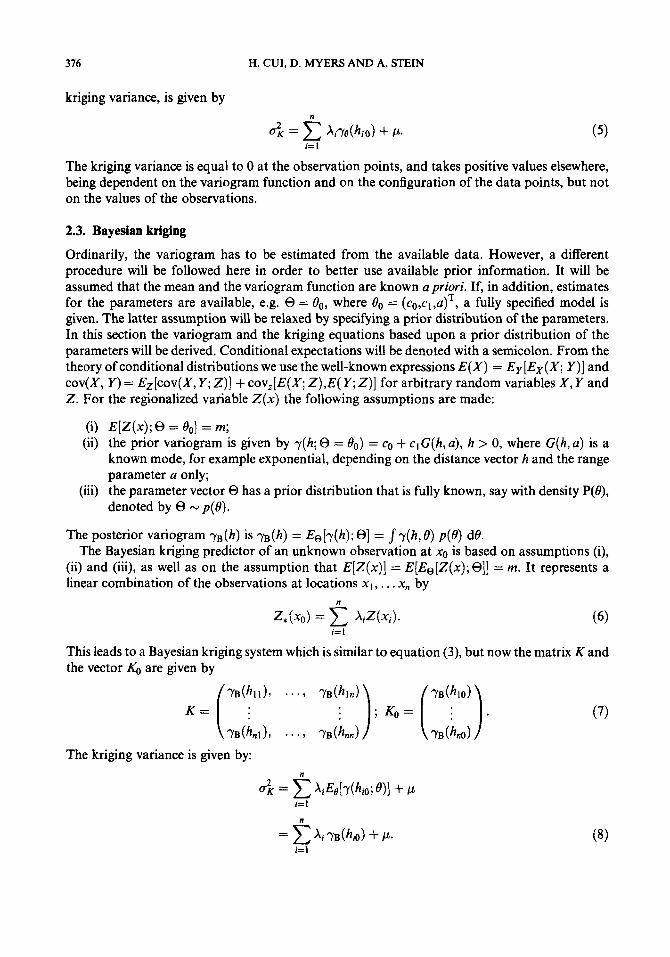
kriging variance, is given by

The kriging variance is equal to 0 at the observation points, and takes positive values elsewhere, being dependent on the variogram function and on the configuration of the data points, but not on the values of the observations.

2.3. Bayesian kriging

Ordinarily, the variogram has to be estimated from the available data. However, a different procedure will be followed here in order to better use available prior information. It will be assumed that the mean and the variogram function are known a priori. If, in addition, estimates for the parameters are available, e.g. Q = do, where 0, = ( C ~ , C ~ , U ) ~ , a fully specified model is given. The latter assumption will be relaxed by specifying a prior distribution of the parameters. In this section the variogram and the kriging equations based upon a prior distribution of the parameters will be derived. Conditional expectations will be denoted with a semicolon. From the theory of conditional distributions we use the well-known expressions E ( X ) = Ey[Ex(X; Y)] and cov(X, Y) = Ez[cov(X, Y; Z)] + cov,[E(X; Z),E( Y; Z)] for arbitrary random variables X , Y and 2. For the regionalized variable Z(x) the following assumptions are made:

(i) E [ Z ( x ) ; B = 6,] = m; (ii) the prior variogram is given by y(h; 8 = 00) = co + clG(h, a), h > 0, where G(h, a) is a

known mode, for example exponential, depending on the distance vector h and the range parameter a only;

(iii) the parameter vector Q has a prior distribution that is fully known, say with density P(0), denoted by 8 N p ( 0 ) .

The posterior variogram yB(h) is y ~ ( h ) = Ee[y(h); Q] = J y ( h , 6 ) p(0 ) do. The Bayesian kriging predictor of an unknown observation at xo is based on assumptions (i),

(ii) and (iii), as well as on the assumption that E ( Z ( x ) ] = E[Ee(Z(x ) ; Q]] = m. It represents a linear combination of the observations at locations xl , . . . xn by

This leads to a Bayesian kriging system which is similar to equation (3), but now the matrix K and the vector KO are given by

yB(hll)> . . ., yB(!ln))

?B(hnl), - . * > 'YB(hnn) yB(hnO)

(%(:lO))

K = ( i KO = (7)

The kriging variance is given by:

EXTENSION OF SPATIAL INFORMATION 377

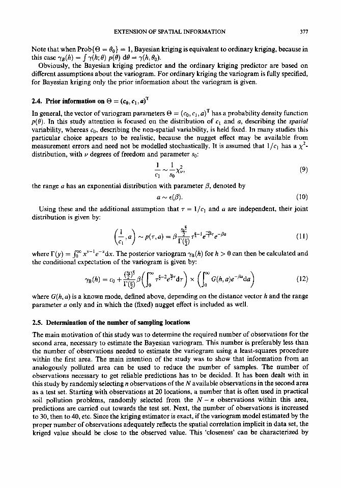
Note that when Prob{B = 0,) = 1, Bayesian kriging is equivalent to ordinary kriging, because in this case yB(h) = J y ( h ; 0) p ( 0 ) d0 = y(h, 0,).

Obviously, the Bayesian kriging predictor and the ordinary kriging predictor are based on different assumptions about the variogram. For ordinary kriging the variogram is fully specified, for Bayesian kriging only the prior information about the variogram is given.

2.4. Prior information on 0 = (cg, c1, a)T

In general, the vector of variogram parameters 0 = (co, cl, a)T has a probability density function p ( 0 ) . In this study attention is focused on the distribution of c1 and a, describing the spatial variability, whereas cot describing the non-spatial variability, is held fixed. In many studies this particular choice appears to be realistic, because the nugget effect may be available from measurement errors and need not be modelled stochastically. It is assumed that l/cl has a x2- distribution, with v degrees of freedom and parameter SO:

the range a has an exponential distribution with parameter /3, denoted by

a 4/31. (10) Using these and the additional assumption that T = l /c l and a are independent, their joint

distribution is given by:

where r(y) = Jp x”-le-xdx. The posterior variogram yB(h) for h > 0 can then be calculated and the conditional expectation of the variogram is given by:

where G(h, a) is a known mode, defined above, depending on the distance vector h and the range parameter a only and in which the (fixed) nugget effect is included as well.

2.5. Determination of the number of sampling locations

The main motivation of this study was to determine the required number of observations for the second area, necessary to estimate the Bayesian variogram. This number is preferably less than the number of observations needed to estimate the variogram using a least-squares procedure within the first area. The main intention of the study was to show that information from an analogously polluted area can be used to reduce the number of samples. The number of observations necessary to get reliable predictions has to be decided. It has been dealt with in this study by randomly selecting n observations of the N available observations in the second area as a test set. Starting with observations at 20 locations, a number that is often used in practical soil pollution problems, randomly selected from the N - n observations within this area, predictions are carried out towards the test set. Next, the number of observations is increased to 30, then to 40, etc. Since the kriging estimator is exact, if the variogram model estimated by the proper number of observations adequately reflects the spatial correlation implicit in data set, the kriged value should be close to the observed value. This ‘closeness’ can be characterized by

378 H. CUI, D. MYERS AND A. STEIN

following three statistics - the mean error (E), the mean squared error (MSE), and the variance of the reduced error uiE - defined as

1 " i=l

E = - c ( z * ( x i ) - .(Xi))

where z*(xi) is the prediction and z(xi) the observation at the ith test point. The mean error t should be close to zero, the MSE value should be small, whereas the niE statistic should be close to one and is used to see whether the prior information about the variogram is correct. Actually

also depends on the configuration of the observation locations and on the location where a prediction is to be carried out. According to the properties of these three statistics, we can use these three statistics to measure the influence of the number of observations on the quality of the predictions. We summarize these statistics in the vector A = (E,(MSE,C&~)~. When the number of observations reaches 100-150 points, the variogram within the second area could be directly determined.

For ordinary kriging we have to estimate the variogram from the data using a least-squares criterion. In the second area, this variogram may then be used as well. Since we have access to all the data locations in the second area, we may modify the Bayesian variogram stepwise, and we can analyse the use of the modified prior variogram by comparing it to ordinary kriging.

3. RESULTS

3.1. Description of the study area

In the south-eastern part of the Netherlands, an area including the municipalities of Budel and Weert is polluted with cadmium and zinc (Stein, 1993). Cadmium is not usually found in nature, except for very small amounts in certain fungi. Pollution levels, the so-called A-, B- and C-levels, are used to decide between successive stages in environmental policies. If observations below the A-level are collected during a first global inventory, the area is considered uncontaminated. The B-level serves as an indicator to start an additional detailed research; if observations above the B- level are obtained, a detailed investigation follows. If observations above the C-level are obtained the area has to be remediated, by excavating the polluted soil, by cleaning it, or by using an in situ treatment.

The pollution in this area has been caused by nearby zinc forges, which have been under operation for decades. One forage is located in Budel, and is still under operation; other forges are located across the Belgian border. The production process has been improved during the early seventies, being considerably less contaminating nowadays. Because cadmium has the highest risk for public health, it was taken as the leading indicator.

The data cover an area of approximately 60 km2, of which approximately 18 kg2 is situated in the municipality of Budel and 42km2 in the municipality of the Weert, which is a larger municipality with more inhabitants (Figure 1). During a survey carried out in allotment gardens during the second half of the 1980s, 2020 observations were collected on the cadmium content of

EXTENSION OF SPATIAL INFORMATION 379

Noithing ( k m )

Bude 1

Figure I . Overview of the cadmium concentrations collected from allotment gardens within the Budel-Weert area. The zinc forge is situated at the south-westem edge of Budel

the topsoil, i.e. 0-30cm below the surface. Samples consisted of a mixture of 8-10 individual samples from one garden.

A major issue concerns extension of the investigation to seven neighbouring municipalities, and the question was raised whether so many observations were again necessary. Prior information available from the sampled municipalities might be useful. To mimic this situa- tion, it was assumed first that only the Budel data were available, being more heavily polluted because of the closeness of the forge, and that the data at Weert were to be predicted. This simulates extension of spatial information with actual measurements being available to validate the predictions.

3.2. Summary statistics and spatial variability

In the Budel area, the observations ranged from 0.4 to 6.9 mg kg-' dry matter, with average calcium value equal to 1.49 mg kg-' and (individual) standard deviation to 0.79. The average value is well below the modified B-level, in this area set equal to 2.5 mg kg-'. However, the B-level is exceeded at several locations, especially at those close to the polluting source. A normal probability plot of the observations is given in Figure 2. In order to interpolate data to unvisited locations, local neighbourhoods are used, since data at a larger distance do not contribute substantially to the value and the precision of the predictions. In this study, for both Bayesian kriging and ordinary kriging, local neighbourhoods with a maximum of 8 data points and a minimum of 2 data points have been used.

The variogram model chosen for Budel is a Gaussian model with parameter vector 8 =(0.3,0.8,3.0)T, which are the values for nugget, sill and range, respectively. This will be taken as the prior variogram for the Weert area. In order to choose the proper prior distribution of the variogram parameters, we randomly choose subsets from data in Budel, and use each subset Dj to estimate the variogram which is co + cf Gau(a'), where Gau(a') denotes the Gaussain

380

i

0s

0 8

0 7

0 6

0 5

0 4

0 3

02

0 1

0

H. CUI, D. MYERS AND A. STEIN

Probability Plot

0 2 4 6

Figure 2. Normal probability plot of the cadmium data in the Budel-Weert area. Also shown is the applied B-level

function with parameter a'. In this way we get random number sequences {ci}, {d} . Empirically, they have following distributions

that is, the prior distributions of the variogram parameters cI and a, respectively, to be applied in the Weert area have the form (14). Hence the variogram used in the Weert area is

r(h; 6 ) = 0.2 + cl e-(lhl/~)', for h > o (15)

where for the bivariate distribution of the vector 0 = (1 /cl, a)T it is assumed that

Using the above prior information, Bayesian kriging was used to predict the observations in different locations in the Weert area (Table I). The statistics vector A = (E, MSE, a',E)T defined in (13) was equal to (-0.00262,0-138,0.425)T. Recall that the MSE value is equal to the average of the squared differences between the predictions and the observations. Since the value of E is small, the predictor is noted to be unbiased, although on the average the predictions are slightly too low. Also, a relatively low MSE value is obtained, compared to the mean value. However, the & value is relatively far below 1, showing that a substantial part of the error is not measured by the prediction error variance. The statistics vector A obtained with ordinary kriging in which the variogram estimated from data in Budel is used is equal to A = (0.00882, 0.1254, 0-334)=. Comparing this with the one obtained by Bayesian kriging, it can be seen that the E for Bayesian kriging is closer to zero than that for ordinary kriging and the dE for Bayesian kriging is closer to 1 than uiE obtained with ordinary kriging. This implies that the Bayesian kriging result is better than the ordinary kriging which uses a variogram estimated from data in Budel. Since Bayesian kriging is kriging which uses the posterior variogram as the variogram, it means that the posterior variogram is more precise than the prior variogram. Also, a sample variogram

EXTENSION OF SPATIAL INFORMATION 38 1

Table I. The values for the mean error c, the mean squared error MSE and the residual variance & obtained with ordinary and Bayesian kriging for different

parameter vectors and distributions

Parameter vector F,

CO

Ordinary Bayesian Ordinary Bayesian Ordinary Bayesian Ordinary Bayesian Ordinary

0.3 0.2 0.2 0.17 0.17 0.17 0.18 0.17 0.2

1 lc1 a c

0.8 3.0 0.00882 1 2 3x10 40.2) -0.00626 0.13 5.5 -007723 1 2 ? x i 5 ~(0.18) -0.00642 0.2 5.0 -0.00734 5x:2 40.2) -0.00179 0.17 4.0 -040237 1 2 2x13 ~(0.25) 0.00030 0.2 3.2 0.00061

MSE

0.1254 0.1384 0.1506 0.1414 0.1387 0.1383 0.1343 0.1344 0.1354

ORE’

0.334 0.425 1.734 0.462 1.675 0.575 0.771 0.697 0.581

c(b) is the exponential distribution with parameter b

was calculated for the Weert area, using only the 20 observations. The variogram model estimated from the sample variogram is a Gaussian one with parameter vector 0 = (co, cl, a)T = (0.2, 0.13, 5.5)T. If we compare the statistics vector A = (0.000608, 0.1354, 0-581)T, obtained with ordinary kriging, with the A obtained by Bayesian kriging, it is noticed that the MSE value does not change substantially, that the change in the value for E is relatively large, which is not so important concerning the practical implications, and that the main change is observed in the ukE value, which is now closer to 1. This shows that the predictions obtained with Bayesian kriging are acceptable, but slightly inferior, compared to those obtained with ordinary kriging.

3.3. Updating prior information

Since we use the Budel data to model the variogram and then use this variogram to set the prior distribution for the parameters of the variogram in the Weert area, it becomes evident that the prior distribution of the parameters for the variogram had to be updated after taking observations in the Weert area. Upon taking 20 observations, that is, taking the subset containing 20 samples from the Weert area, the sample variogram is computed. Using this variogram, the values in the test locations are estimated. The vector A = ( E , MSE, uRE) is equal to (-0.0772,0-1506, 1.7348)T. On the basis of the parameter vector for this variogram, the prior distribution of the arameters was modified by adjusting the degrees of freedom and the parameter so of l/soxv such that the expectation of c1 is close to 0.1 3, and adjusting the parameter ,f3 of the exponential model such that the mean of range a is close to 5.0. That is, the modified prior distribution of (l/cl,a)T is equal to

2 T

4

e.g. with l/cl following a xz distribution with degrees of freedom v equal to 15 and parameters so equal to 2 and the range a following an exponential distribution with parameter equal to 0.2. Using the modified prior distribution, the vector A is equal to A = (-0.00642,0.1414, 0.4624)T. Comparing this value with A = (-0.00626, 0.138, 0.425)T obtained with the prior distribution (14), it is noticed that only the value of is improved slightly. This shows that the information obtained from 20 observations is not sufficient to substantially modify the prior distribution of variogram parameters.

382 H. CUI, D. MYERS AND A. STEIN

.. **:

: '. a.0

-1 '

Figure 3. The observation locations in the Weert area, showing both the original observation points as well as the locations of the test sets of different sizes

Next, another 40 observations were added to the previous 20 observations, i.e. a subset was taken containing 60 samples from data in Weert. Using these 60 observations to estimate the variogram model, a Gaussian model was obtained with parameter vector €3 = (co, cl, = (0.17,0.2, 5-O)T. The prior distribution (14) was modified in a similar way as before, using these parameters, to obtain

(+) N ix :2 x 4 0 . 2 ) .

When this was applied as the prior distribution, the statistics vector A equal to (-0.00179,0.138, 0-575)T was obtained. Comparison with the vector A = (-0~00626,0~130,0~425)T obtained with the unmodified prior distribution (14) reveals that using the modified prior distribution gives a okE value closer to 1, and an E value closer to 0. This shows that the predictions obtained with Bayesian kriging by using a modified prior distribution improves those obtained by using prior distribution without modification.

After adding another 80 observations in the Weert area to the previous 60 observations, the variogram could be estimated. It shows a Gaussian model with parameter vector €3 = (co, c1, = (0.17,0.17,4-O)T. Now the prior distribution (14) was modified in the same way as before, yielding as the modified prior distribution:

Using this as a prior distribution for Bayesian kriging gives A = (0.000302, 0-134, 0~697)~ . Comparing these values with those obtained with (14) it can be seen that Bayesian kriging shows much better results than those obtained previously. This shows that the modified prior information of variogram parameters works well in the Weert area.

Comparing the ordinary kriging with Bayesian kriging, we notice that ordinary kriging, using a

EXTENSION OF SPATIAL INFORMATION 383

Table 11. The values for the mean error e, the mean squared error MSE and the residual variance & as a function of the

number of observations in the Weert area

N € MSE dE 20 40 60 80

100 120 140 160 180 350

-0.07344 -0.03794 -0.02934 -002672 -0.01 49 1

000489 0-0073 1 040627 0.00871

-0.001 10

0.1418 0.1323 0.1313 0-1311 0.1251 01218 01212 0.1233 0.1241 0.1359

042 19 0.4146 0.4228 0.4253 0.4104 04059 04089 0.4178 04216 0.4655

Gaussian variogram with parameter vector 0 = (cg, cl , @)T = (0.1 7,0.2, 5.0)T estimated from the subset containing 60 observations in the Weert area, yields A = (-0.00734, 0.139, 1-675).T Comparing this vector with A = (-0.00179, 0.138, 0.575) obtained with Bayesian kriging we note almost the same MSE value, but relatively large differences in c and dE. Bayesian kriging yields less biased predictions as well as a oiE value closer to 1 than the dE obtained with ordinary kriging.

Using the variogram obtained from the subset containing 140 observations in Weert, ordinary kriging gives as a result the vector A = (-0.00237,0-133, 0.771)T. Comparing these values with A = (0~000302,0~134, 0-697)T, obtained with Bayesian kriging, it can be seen that the 6 values are both close to 0, that the MSE values are practically the same but that the & value is higher for ordinary kriging than for Bayesian kriging. This shows that ordinary kriging is superior to Bayesian kriging if sufficient observations are available to properly estimate the variogram.

As a next step we determined the size for a minimum data set to appropriately estimate the variogram. To do so, sub-data sets with 20 to 180 samples were selected randomly from the data available in Weert (Table 11). When the sample size increases from 20 to 140, the MSE value decreases, but when the sample size further increases, the MSE value increases as well, indicating that the number of observations to get the most reliable predictions in this study is about 140. This number has been used in the subsequent analysis. In contrast, the mean error c and the residual standard error dE do not show any particular trend. If the number of observations is too small to estimate the variogram, reliable predictions can be obtained only with Bayesian kriging. Taking additional samples after 140 observations does not produce any substantial benefit.

4. DISCUSSION

The main purpose of this study was to analyse the use of spatial information from one area into another. Bayesian kriging offers the opportunity to carry out kriging, even if the number of data is insufficient to properly estimate the variogram. In contrast, ordinary kriging is possible only when sufficient data are available to properly estimate the variogram. Actually, the variogram in Weert was available, and Bayesian kriging was compared with ordinary kriging. Bayesian kriging gives predictions of approximately the same precision as ordinary kriging. Therefore it is concluded that prior information from the first area can be applied in the second area. Of course, ordinary kriging should be better than Bayesian kriging, because the most reliable data

384 H. CUI. D. MYERS AND A. STEIN

are used for estimating the variogram. However, if only 60 data were collected from the second area, ordinary kriging is not better than Bayesian kriging, and hence Bayesian kriging is seen to give reliable results. If it is too elaborate to take sufficient samples to estimate the variogram, a reduction of necessary sampling of at least 50 per cent is allowed.

This paper highlights several advantages and limitations of using prior variogram information for Bayesian kriging. We compared it with the use of ordinary kriging. We have applied one, rather simple, model to describe the distribution of the variogram parameters. Additional studies are needed to determine whether this model can be further refined and extended.

It was possible to use information from one area and apply it to another area. The most obvious gain is that within the second area, the number of observations may be far less than the number of 100-1 50 proposed by Webster and Oliver. This may hold for pollution studies that are similar with respect to pollutant and deposition, but not for completely different studies. In the example shown in this study, cadmium was deposited in the two areas under fairly similar conditions, spread being mainly caused by wind deposition, yielding a diffuse contamination. One may expect, though, different conclusions for areas that are contaminated through groundwater, acidic deposition, or through wilful contamination at several isolated spots in an area, which is further spread through human activities.

REFERENCES

Abrahamsen, P. (1992). ‘Bayesian kriging for seismic depth conversion of a multi-layer reservoir’, in Soares,

Boekhold, A. E. and van der Zee, S. E. A. T. M. (1992). ‘Significance of soil chemical heterogeneity for

Feller, W. (1968). An Introduction to Probability Theory and its Applications, Third edn, Wiley, New York. Finke, P. A. and Stein, A. (1994). ‘Application of co-kriging and disjunctive kriging to optimize fertilizer

additions on a field scale’, Geoderma, 62, 247-263. Flatman, G. T., Englund, E. J. and Yfantis, A. A. (1988). ‘Geostatistical approaches to the design of sampling

regimes’, in Keith, L. H. (ed), Principles of EnvironmentaISampling, American Chemical Society, pp. 73-84. Kitanidis, P. K. (1986). ‘Parameter uncertainty in estimation of spatial functions: Bayesian analysis’, Water

Resources Research, 22, 499-507. Matheron, G. (1971). ‘The theory of regionalized variables and its applications’, Les Cahiers du Centre de

Morphologie Mathkmatigue, No. 5 . Ecole des Mines de Paris, Paris. Myers, D. E. (1988). ‘Multivariable geostatistical analysis for environmental monitoring’, Science de la

Terre, 27, 41 1-527. Nhu D. Le and Zidek, J. V. (1992). ‘Interpolation with uncertain spatial covariances: A Bayesian alternative

to kriging’, Journal of Multivariate Analysis, 43, 35 1-374. O’Hagan, A. (1978) ‘Curve fitting and optimal design for prediction (with discussion), Journal of the Royal

Statistical Society, Series B, 40, 1-42. O’Hagan, A. (1991). ‘Some Bayesian numerical analysis’, in Bernado, J. M. (ed), Bayesian Statistics 4,

Oxford University Press, pp. 1-17. Omre, H. and Halvorsen, K. B. (1989). ‘The Bayesian bridge between simple and universal Kriging’,

Mathematical Geology, 21, 767-786. Staritsky, I. G., Sloot, P. and Stein, A. (1992). ‘Spatial variability of cyanide soil pollution on former

galvanic factor premises’, Water, Air and Soil Pollution, 61, 1-16. Stein, A., Hoogerwerf, M. and Bouma, J. (1988). ‘Use of soil map delineations to improve (co-)kriging of

point data on moisture deficits’, Geoderma, 43, 163-177. Stein, A. (1994). ‘The use of pior information in spatial statistics’, Geoderma, 62, 199-216. Switzer, P. (1977). ‘Estimating of spatial distributions from point sources with application to air pollution

measurement’, Bulletin of the International Statistical Institute, XLVII, (2) 122-137. Webster, R. and Oliver, M. A. (1993). ‘How large a sample is needed to estimate the regional variogram

adequately?, in Soares, A. (ed), Geostatistics Trdia ’92, Kluwer, Dordrecht, pp. 155-166. Zhu, H. and Journel, A. (1991). ‘Mixture of populations’, Mathematical Geology, 23, 647-671.

A. (ed), Geostatistics Trdia ’92, Kluwer, Dordrecht, pp. 385-398.

spatial behavior of cadmium in field soils’, Soil Sci. SOC. Am J., 56, 747-754.