Atmos. Chem. Phys., 12, 2357–2380, 2012www.atmos-chem-phys.net/12/2357/2012/doi:10.5194/acp-12-2357-2012© Author(s) 2012. CC Attribution 3.0 License.

AtmosphericChemistry

and Physics

Five blind men and the elephant: what can the NASA Aura ozonemeasurements tell us about stratosphere-troposphere exchange?

Q. Tang1,2 and M. J. Prather1

1Department of Earth System Science, University of California, Irvine, California, 92697, USA2Department of Biological and Environmental Engineering, Cornell University, Ithaca, New York, 14853, USA

Correspondence to:Q. Tang (qtang@cornell.edu)

Received: 17 September 2011 – Published in Atmos. Chem. Phys. Discuss.: 29 September 2011Revised: 10 January 2012 – Accepted: 19 January 2012 – Published: 2 March 2012

Abstract. We examine whether the individual ozone (O3)measurements from the four Aura instruments can quantifythe stratosphere-troposphere exchange (STE) flux of O3, animportant term of the tropospheric O3 budget. The level 2(L2) Aura swath data and the nearly coincident ozone son-des for the years 2005–2006 are compared with the 4-D,high-resolution (1◦×1◦

×40-layer× 0.5 h) model simulationof atmospheric ozone for the same period from the Univer-sity of California, Irvine chemistry transport model (CTM).The CTM becomes a transfer standard for comparing in-dividual profiles from these five, not-quite-coincident mea-surements of atmospheric ozone. Even with obvious modeldiscrepancies identified here, the CTM can readily quan-tify instrument-instrument biases in the tropical upper tropo-sphere and mid-latitude lower stratosphere. In terms of STEprocesses, all four Aura datasets have some skill in iden-tifying stratosphere-troposphere folds, and we find severalcases where both model and measurements see evidence ofhigh-O3 stratospheric air entering the troposphere. In manycases identified in the model, however, the individual Auraprofile retrievals in the upper troposphere and lower strato-sphere show too much noise, as expected from their lowsensitivity and coarse vertical resolution at and below thetropopause. These model-measurement comparisons of in-dividual profiles do provide some level of confidence in themodel-derived STE O3 flux, but it will be difficult to integratethis flux from the satellite data alone.

1 Introduction

Quantifying and understanding the causes of changes inthe tropospheric ozone (O3) burden are important topicsfor climate research and environmental studies, as ozone is

a major greenhouse gas and plays a key role in the tro-pospheric chemistry. Besides obvious factors such as an-thropogenic emissions of ozone precursors (Gauss et al.,2006; Hoor et al., 2009; Myhre et al., 2011; Holmeset al., 2011) and natural emissions of biogenic volatile or-ganic compounds (Atkinson and Arey, 2003; Shao et al.,2009), stratospheric ozone influx has been identified as amajor driver of tropospheric ozone changes (Roelofs andLelieveld, 1997; Fusco and Logan, 2003; Terao et al., 2008;Hsu and Prather, 2009). There are large uncertainties inthe estimates of global annual stratosphere-troposphere ex-change (STE) of ozone flux either derived from observations(450 Tg(O3) yr−1 (range, 200–870) (Murphy and Fahey,1994), 510 Tg(O3) yr−1 (450–590) (Gettelman et al., 1997),550±140 Tg(O3) yr−1 (Olsen et al., 2001)) or from modelsimulations (e.g.,Denman et al., 2007, Table 7.9 and ref-erences therein). There are also disagreements in terms ofthe magnitude and phase of the annual cycle as well as thegeographical patterns (Gettelman et al., 1997; Roelofs andLelieveld, 1997; Olsen et al., 2004; Hsu et al., 2005; Hsu andPrather, 2009). The large uncertainties and differences in theassessments of the STE O3 budget are partly due to the differ-ent definitions and diagnostic methods used in these studiesand partly due to the great temporal and spatial variances ofthe STE flux.

The four Earth Observing System (EOS) Aura satel-lite ozone measurements (High Resolution Dynamics LimbSounder (HIRDLS), Microwave Limb Sounder (MLS),Ozone Monitoring Instrument (OMI), and TroposphericEmission Spectrometer (TES)) plus the coincident ozonesondes flown for calibration/validation of the satellite in-struments comprise a somewhat overlapping set of five dif-ferent ozone measurements. We merge these five with the

Published by Copernicus Publications on behalf of the European Geosciences Union.

2358 Q. Tang and M. J. Prather: Aura measurements and cross-tropopause ozone flux

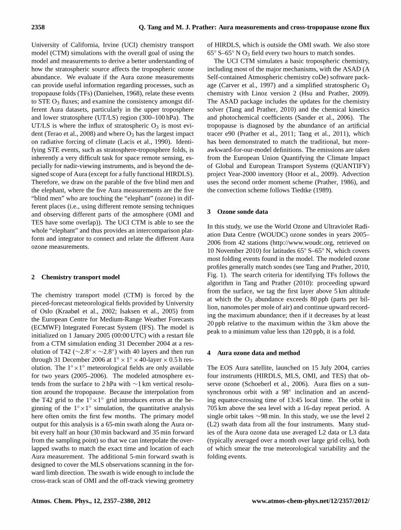
University of California, Irvine (UCI) chemistry transportmodel (CTM) simulations with the overall goal of using themodel and measurements to derive a better understanding ofhow the stratospheric source affects the tropospheric ozoneabundance. We evaluate if the Aura ozone measurementscan provide useful information regarding processes, such astropopause folds (TFs) (Danielsen, 1968), relate these eventsto STE O3 fluxes; and examine the consistency amongst dif-ferent Aura datasets, particularly in the upper troposphereand lower stratosphere (UT/LS) region (300–100 hPa). TheUT/LS is where the influx of stratospheric O3 is most evi-dent (Terao et al., 2008) and where O3 has the largest impacton radiative forcing of climate (Lacis et al., 1990). Identi-fying STE events, such as stratosphere-troposphere folds, isinherently a very difficult task for space remote sensing, es-pecially for nadir-viewing instruments, and is beyond the de-signed scope of Aura (except for a fully functional HIRDLS).Therefore, we draw on the parable of the five blind men andthe elephant, where the five Aura measurements are the five“blind men” who are touching the “elephant” (ozone) in dif-ferent places (i.e., using different remote sensing techniquesand observing different parts of the atmosphere (OMI andTES have some overlap)). The UCI CTM is able to see thewhole “elephant” and thus provides an intercomparison plat-form and integrator to connect and relate the different Auraozone measurements.

2 Chemistry transport model

The chemistry transport model (CTM) is forced by thepieced-forecast meteorological fields provided by Universityof Oslo (Kraabøl et al., 2002; Isaksen et al., 2005) fromthe European Centre for Medium-Range Weather Forecasts(ECMWF) Integrated Forecast System (IFS). The model isinitialized on 1 January 2005 (00:00 UTC) with a restart filefrom a CTM simulation ending 31 December 2004 at a res-olution of T42 (∼2.8◦

× ∼2.8◦) with 40 layers and then runthrough 31 December 2006 at 1◦

×1◦×40-layer× 0.5 h res-

olution. The 1◦×1◦ meteorological fields are only availablefor two years (2005–2006). The modeled atmosphere ex-tends from the surface to 2 hPa with∼1 km vertical resolu-tion around the tropopause. Because the interpolation fromthe T42 grid to the 1◦×1◦ grid introduces errors at the be-ginning of the 1◦×1◦ simulation, the quantitative analysishere often omits the first few months. The primary modeloutput for this analysis is a 65-min swath along the Aura or-bit every half an hour (30 min backward and 35 min forwardfrom the sampling point) so that we can interpolate the over-lapped swaths to match the exact time and location of eachAura measurement. The additional 5-min forward swath isdesigned to cover the MLS observations scanning in the for-ward limb direction. The swath is wide enough to include thecross-track scan of OMI and the off-track viewing geometry

of HIRDLS, which is outside the OMI swath. We also store65◦ S–65◦ N O3 field every two hours to match sondes.

The UCI CTM simulates a basic tropospheric chemistry,including most of the major mechanisms, with the ASAD (ASelf-contained Atmospheric chemistry coDe) software pack-age (Carver et al., 1997) and a simplified stratospheric O3chemistry with Linoz version 2 (Hsu and Prather, 2009).The ASAD package includes the updates for the chemistrysolver (Tang and Prather, 2010) and the chemical kineticsand photochemical coefficients (Sander et al., 2006). Thetropopause is diagnosed by the abundance of an artificialtracer e90 (Prather et al., 2011; Tang et al., 2011), whichhas been demonstrated to match the traditional, but more-awkward-for-our-model definitions. The emissions are takenfrom the European Union Quantifying the Climate Impactof Global and European Transport Systems (QUANTIFY)project Year-2000 inventory (Hoor et al., 2009). Advectionuses the second order moment scheme (Prather, 1986), andthe convection scheme followsTiedtke(1989).

3 Ozone sonde data

In this study, we use the World Ozone and Ultraviolet Radi-ation Data Centre (WOUDC) ozone sondes in years 2005–2006 from 42 stations (http://www.woudc.org, retrieved on10 November 2010) for latitudes 65◦ S–65◦ N, which coversmost folding events found in the model. The modeled ozoneprofiles generally match sondes (seeTang and Prather, 2010,Fig. 1). The search criteria for identifying TFs follows thealgorithm in Tang and Prather(2010): proceeding upwardfrom the surface, we tag the first layer above 5 km altitudeat which the O3 abundance exceeds 80 ppb (parts per bil-lion, nanomoles per mole of air) and continue upward record-ing the maximum abundance; then if it decreases by at least20 ppb relative to the maximum within the 3 km above thepeak to a minimum value less than 120 ppb, it is a fold.

4 Aura ozone data and method

The EOS Aura satellite, launched on 15 July 2004, carriesfour instruments (HIRDLS, MLS, OMI, and TES) that ob-serve ozone (Schoeberl et al., 2006). Aura flies on a sun-synchronous orbit with a 98◦ inclination and an ascend-ing equator-crossing time of 13:45 local time. The orbit is705 km above the sea level with a 16-day repeat period. Asingle orbit takes∼98 min. In this study, we use the level 2(L2) swath data from all the four instruments. Many stud-ies of the Aura ozone data use averaged L2 data or L3 data(typically averaged over a month over large grid cells), bothof which smear the true meteorological variability and thefolding events.

Atmos. Chem. Phys., 12, 2357–2380, 2012 www.atmos-chem-phys.net/12/2357/2012/

Q. Tang and M. J. Prather: Aura measurements and cross-tropopause ozone flux 2359

0 100 200 300 400

70

100

158

251

398

631

1000

O3 (ppb)

Pre

ssur

e (h

Pa)

−0.1 −0.05 0 0.05 0.1

30

50

70

100

158

251

398

631

1000

TES Averaging Kernel

TES aPTESCTM intpCTM w/ AK

Surf.−700700−250250−100100−30

(a)

(b)

Fig. 1. Comparisons between TES a priori (green), TES (red), linearly interpolated CTM on TES levels (blue) and convolved CTM (black)ozone profiles (a, unit: ppb) and the corresponding TES averaging kernel (AK,b) as a function of pressure at 9.5◦ S, 295.0◦ E on 25 August2005. In panel(a), dashed magenta line shows the e90 tropopause of 99 hPa. The AK for different pressure ranges are represented by solidlines in (b): blue for surface–700 hPa, green for 700–250 hPa, red for 250–100 hPa, and cyan for 100–30 hPa. The dashed black line in(b)shows the zero line. The DOFS for the troposphere and the whole atmosphere are 1.5 and 4.0, respectively.

Longitude

z* (k

m)

60

60

60

60

6060

60

60

60

60

80

8080

8080

80

80

8080

150150

150

130 140 150 160 170 1800

2

4

6

8

10

12

14

16

18

20

Longitude

606060

60

60

60

60

60

60

60

60

80

8080

80

80

8080

80

150 150

150

130 140 150 160 170 1800

2

4

6

8

10

12

14

16

18

20

Longitude

606060

60

60

60

60

60

60

60

80

8080

80

80

80

80

80

80

150150

150

130 140 150 160 170 1800

2

4

6

8

10

12

14

16

18

20

−100

−50

0

50

100

150

200

250

300O3 (ppb)

(a) (c)(b)31/01/2005 00:00 UTC 31/01/2005 02:00 UTC 31/01/2005 04:00 UTC

Fig. 2. Pressure altitude (z∗) by longitude (120◦ E–190◦ E) plots of simulated ozone (colors: blue shows low values, red high values, unit:ppb) at 29.5◦ N on 31 January 2005(a) 00:00 UTC,(b) 02:00 UTC, and(c) 04:00 UTC. The thin black contour lines represent ozone of60, 80, and 150 ppb. The thick black contour lines define the 100-ppb ozone surface (approximately the tropopause). The magenta squarescorrespond to the same CTM grid box.

4.1 HIRDLS

HIRDLS observes the atmosphere in limb direction at 21infrared channels from 6.12 to 17.76 µm (HIRDLS Team,2010). After launch a spacecraft malfunction resulted in∼80 % blockage of its optical path which limited the cov-erage from 65◦ S to 82◦ N, missing the Antarctic. With itslimited field of view at one azimuth angle, however, HIRDLScan still retrieve ozone profiles (260–0.5 hPa) with high ver-tical resolution (∼1 km). These continuous observations atone azimuth can facilitate studies on short-lived processes(e.g., gravity waves (Alexander et al., 2008)) and possiblyTFs. Because of this failure, HIRDLS is not able to measurethe same atmospheric profile as the rest Aura instrumentswithin 15 min, but instead views the same location 84 min

earlier than MLS at night and 17◦ to the east of the MLStrack during the daytime.

We use version 5 (v5.00.00) HIRDLS ozone data in thisstudy. The data with negative “O3Precision” or earth-ward from the nearest and above the “CloudTopPressure”are screened out. The “gradient filter” is not applied, be-cause high vertical ozone gradient exists when tropopausefolds occur. Note that without the “gradient filter” someunrealistically high ozone spikes are not excluded (seeFigs.3g and4g).

www.atmos-chem-phys.net/12/2357/2012/ Atmos. Chem. Phys., 12, 2357–2380, 2012

2360 Q. Tang and M. J. Prather: Aura measurements and cross-tropopause ozone flux

0 100 200 300 400

70

100

158

251

398

631

1000

O3 (ppb)Pr

essu

re (h

Pa)

WOUDCCTM

0 90 180 270 360−90

−60

−30

0

30

60

90

Latit

ude

0 90 180 270 360−90

−60

−30

0

30

60

90

Longitude

Latit

ude

0 90 180 270 360−90

−60

−30

0

30

60

90

Longitude

0 10 20 30 40 50 60

−34 −12 9 31 53215147100 68 46

Pres

sure

(hPa

)

−34 −12 9 31 53215147100 68 46

−55 −33 −8 17 46261196147110 83 62

Pres

sure

(hPa

)

−55 −33 −8 17 46261196147110 83 62

−59 −36 −9 15 41 62

70100

158

251

398

631

1000

Latitude

50 100 150 200

−59 −36 −9 15 41 62

70100

158

251

398

631

1000

Latitude

Pres

sure

(hPa

)

(i) (j)

TCO (DU)(e) (f)

(g) (h)

O3 (ppb)

(a)

(b)

(c) (d)

OMI CTM

MLS CTM

TES

CTMHIRDLS

CTM

Fig. 3. Comparisons between sonde and Aura ozone swaths with CTM for 23 March 2005.(a) WOUDC sonde (blue, 05:26 UTC) vs. CTM(red, 06:00 UTC) profile (unit: ppb) at Hong Kong (22.3◦ N, 114.2◦ E, station code 344).(b) The locations of available Aura measurements(on the CTM grid) during 05:00–06:00 UTC. HIRDLS: black crosses, MLS: cyan crosses, TES: red crosses, OMI: green dots, sonde locationin (a): the large black cross. Comparisons for Aura (left) vs. exact matching CTM results (right) swaths:(c) vs. (d) for OMI; (e) vs. (f) forMLS; (g) vs. (h) for HIRDLS; (i) vs. (j) for TES. We compare latitude-by-longitude TCO (unit: DU) for OMI swaths, pressure-by-latitudeO3 molar ratios (0◦–180◦ E, unit: ppb) for HIRDLS, MLS, and TES. The black lines in(e)–(j) represent the e90 tropopause.

4.2 MLS

MLS measures stratospheric and upper tropospheric ozoneusing microwave limb sounding technology at 240 GHz(Schoeberl et al., 2006; Waters et al., 2006). Although theversion 3.3 standard O3 product has doubled vertical reso-lution and an enlarged pressure range, we opt here for ver-

sion 2.2 data, as oscillations appear in the tropical uppertroposphere (UT) profiles of version 3.3, even for monthlymean ozone profiles (Livesey et al., 2011). The verticalresolution of MLS ozone profiles is∼3 km in the UT andstratosphere. The horizontal resolution is∼200 km× 6 km(along-track× cross-track). The precision of single profile is40 ppb at 215–100 hPa (Livesey et al., 2007). We extract the

Atmos. Chem. Phys., 12, 2357–2380, 2012 www.atmos-chem-phys.net/12/2357/2012/

Q. Tang and M. J. Prather: Aura measurements and cross-tropopause ozone flux 2361

scientifically useful data from 215 hPa to 0.02 hPa. Only datawith (1) positive precision, (2) even-numbered “Status”, (3)“Quality” greater than 1.2, and (4) “Convergence” less than1.8 are used in this study.

4.3 OMI

OMI uses a 2-D Charge-Coupled Device to measure thebackscattered solar irradiance from nadir direction at ultra-violet and visible wavelengths (UV-1: 264–311 nm, UV-2:307–383 nm, VIS: 349–504 nm). The wide cross-orbit swath(2600 km) allows OMI to provide global daily coverage(OMI Team, 2009). In this study, we use the OMO3PR V003ozone profiles with a horizontal resolution of 13 km×48 km(along-track× cross-track) and 18 vertical layers from thesurface to 0.3 hPa (de Haan and Veefkind, 2009). In thetroposphere, the vertical resolution is very coarse (3–6 lay-ers) and thus OMI cannot resolve vertical structures such asTFs. OMI does provide useful information about the tropo-spheric column, including its enhancements in regions withTFs (Tang and Prather, 2010). The OMI tropospheric columnozone (TCO) is derived by applying the tropopause heightoutput from the UCI CTM to the OMI ozone profiles.

4.4 TES

TES is a high resolution infrared Fourier transform spectrom-eter with spectral coverage from 650 to 3250 cm−1 at a spec-tral resolution of 0.025 cm−1. It is designed to view the atmo-sphere in both nadir and limb directions with a 5 km×8 kmnadir footprint. The limb scan mode, however, was elim-inated in 2005 to conserve instrument life. The version 4(V004, F0507) nadir global survey standard ozone productis used in this paper. The profiles are reported at 67 pres-sure levels from the surface to 0.1 hPa, but in the tropospherethere are only 1–2 degrees of freedom for the signal (DOFS)(Nassar et al., 2008; Zhang et al., 2010). Ozone profileswhose “SpeciesRetrievalQuality” or “O3CcurveQA” doesnot equal 1 are excluded (Osterman et al., 2009). Some ofthe TES profiles (0.5 %) contain fill values for the averagingkernel (AK), and these are also excluded.

4.5 Methods of mapping modeled ozone profiles ontoreported Aura measurements

The CTM and Aura ozone profiles all have different loca-tions and pressure coordinates. For geographic collocation,we choose without interpolation the 1◦

×1◦ model grid con-taining the centre (for OMI and TES) or the location of thetangent height (for HIRDLS and MLS) of the observation.Temporal differences are accounted for by interpolation be-tween the two half-hour model simulations bounding the ob-servation as described above. The vertical remapping is morecomplex and specific to each instrument. Before compar-ing them, we first map CTM profiles onto the Aura levelseither by linear interpolation in pressure for HIRDLS and

MLS or by convolution with the a priori and averaging ker-nel (AK) (together referred as the satellite operator) for OMIand TES. The “least squares fit” method recommended byLivesey et al.(2007) is unstable for the lowermost MLS lay-ers, which are particularly important for this paper. Alsoconsidering that HIRDLS and MLS have vertical resolutionscomparable to that of the CTM, we decided to simply inter-polate the CTM profiles onto HIRDLS and MLS levels. ForOMI and TES the satellite operators are applied to the CTMprofiles to account for limited vertical resolution and sensi-tivity of nadir viewing measurements based upon the follow-ing equation (Luo et al., 2007; Worden et al., 2007):

xm = xa+A(xm−xa) (1)

wherexa andA are the a priori and averaging kernel as re-ported in OMI and TES HDF-EOS5 metadata. The mod-eled ozone profiles are first interpolated onto the satellite lev-els. The above equation then transforms the interpolated pro-files xm to the “retrieved” profilesxm, mimicking the verti-cal smoothing of the retrieval process of OMI and TES data.Note thatxm is in Dobson Unit (DU) for OMI and the naturallogarithm of ozone molar ratio for TES.

4.6 Problems with applying satellite operators fornadir-view instruments

TES contains 1–2 DOFS in the troposphere and thus providessome tropospheric profile data but less information than isapparent in the 25 tropospheric pressure levels of their re-trievals (see Fig.1). Given the sparse spatial coverage ofTES in contrast with OMI, we can only infer STE processesfrom the changes in upper tropospheric values. Therefore, inthis study we compare the CTM with TES profiles.

Convolving modeled or sonde profiles with Eq. (1) essen-tially smoothes those profiles vertically and relaxes them to-wards the retrieval a priori. For most regions, this methodworks adequately and smoothes the profiles as expected.In the UT, however, applying the satellite operator cancause unphysically high biases (see Fig.1a and Table1).

Figure1a shows the comparison for one of the TES pro-files in Fig.4i at 9.5◦ S, 295.0◦ E. The TES profile (red line)contains a slight inversion at 630 hPa, determined mainlyby its a priori (green line), and a dispersed fold at 600–200 hPa that is primarily contributed by the TES signal.From 120 hPa to 70 hPa, TES values are almost identical toa priori values. The linearly interpolated CTM profile (blueline) also resolves the two folds, but with larger magnitudes.The modeled profile matches the shape as well as the magni-tude retrieved by TES in the UT. Applying the TES operator,the CTM profile (black line) still has the fold at 630 hPa, butthe vertical gradient becomes smoother and the shape is quitesimilar to the a priori estimate. However, the fold at 400 hPais totally smoothed out and the ozone abundance increasesmonotonically above 400 hPa with a much larger slope thanthat of TES, the TES a priori, or the raw CTM profile in the

www.atmos-chem-phys.net/12/2357/2012/ Atmos. Chem. Phys., 12, 2357–2380, 2012

2362 Q. Tang and M. J. Prather: Aura measurements and cross-tropopause ozone flux

Table 1. Means and root mean squares (RMS) of the exact matching TES and CTM partial ozone columns (unit: DU) of the TES swathshown in Fig.4i covering 31.5◦ S–71.4◦ N with 54 individual profilesa.

Regions CTM (±σ ) CTM* TES CTM′−TES′ CTM* ′

−TES′

Upper Trop. (400 hPa–TPP) 13.1 (±3.1) 16.1 14.1 3.3 3.4Mid Trop. (700–400 hPa) 12.8 (±2.0) 12.1 11.1 1.9 1.7Lower Trop. (surf.–700 hPa) 12.1 (±3.1) 9.9 9.3 2.0 1.6

a Single values are the means, while the differences are the RMS of anomalies (e.g.,CTM′= CTM−CTM). CTM∗ represents the CTM values processed with the TES operator.

UT, resulting in unrealistically large O3 abundances in theUT. Smearing stratospheric information into the troposphereby the TES retrieval process is also noted in other studies(Osterman et al., 2008).

The artificially high bias in the UT introduced by applyingthe TES operator reflects: (i) the model’s high bias relativeto TES in the lower stratosphere, (ii) TES’s coarse verticalresolution around the tropopause, and (iii) the large cross-tropopause ozone gradient. The AK for this particular mea-surement is shown in Fig.1b. It is generally thick, indicatingcoarse vertical resolution. Although data is reported at 67levels, the DOFS of this measurement (i.e., the trace of theAK) are 4.0 for all levels, 1.5 for the troposphere, and 0.5 forthe UT (250–100 hPa). The UT retrievals are strongly influ-enced by the layers at 100–50 hPa and 400–250 hPa, whichhave contributions as large as those of the UT region itself(red lines in Fig.1b). Therefore, the large stratospheric dif-ferences between the TES a priori (green line in Fig.1a) andthe raw CTM profile (blue line in Fig.1a) are smoothed andaliased into the UT, swamping the clear UT signal in themodel, and leading to the high model biases in this region.

Table1 shows the means, standard deviations (σ ), and theroot mean squares (RMS) of the partial columns for TES andmatching CTM profiles for the swath shown in Fig.4i. Thisswath consists of 54 individual profiles, covering 31.5◦ S–71.4◦ N. In the upper troposphere (400 hPa–tropopause), theraw CTM mean (second column) is 7 % smaller than TES(fourth column). After processing with the TES operator, theCTM mean (third column) is enhanced by 3.0 DU (almost1σ ) and becomes 14 % larger than TES. In the middle (700–400 hPa) and lower (surface–700 hPa) troposphere, the CTMmeans using the TES operator become smaller and closer tothe TES means. The RMS of anomalies (column 5 and 6) isincreased by the operator in the UT, but reduced in the middleand lower troposphere.

The results in Table1 are typical and suggest that apply-ing the TES operator causes artificially high biases in the UTover most latitudes. This is also true for OMI, whose verticalresolution is even coarser than TES. One possible solutionfor this problem is to redo the TES retrieval process usingour modeled profiles as the a priori, but this would be an ex-tensive effort beyond the scope of this paper. Because theUT region is greatly affected by the STE processes (Terao

et al., 2008), on which this paper focuses, we decided tocompare the interpolated CTM profiles directly with TES onTES pressure levels in the following case studies (Sect.6.1),and we show results both with and without the TES oper-ator for the rest of the analysis. Our problems when usingsatellite operators highlight the fact that to avoid misusingand/or misinterpreting satellite data, it is important to knowthe sensitivities and resolutions of satellite measurements, es-pecially in regions with large gradients like the tropopause.If the real ozone in the lower stratosphere was actually muchhigher than the retrieval a priori, TES would put too muchozone in the UT similar to the convolved model results.

The artificially high bias of local O3 abundances causedby applying nadir satellite operators in the UT, however, ap-pears to have only a small effect on the tropospheric columnozone (TCO) as shown by the sums of the second and thirdcolumns (38.0 DU vs. 38.1 DU) of Table1. As mentionedabove the TES DOFS in the troposphere are generally greaterthan one (Zhang et al., 2010) and thus give reasonable TCOvalues. Likewise, OMI has typically DOFS of 1 for the tropo-sphere (de Haan and Veefkind, 2009), and its TCO matchesthe simulation in terms of geographical patterns and magni-tudes (Tang and Prather, 2010). Therefore, when comparingthe TCO of TES or OMI with the model results, we processCTM profiles with the satellite operators.

5 Temporal and spatial scales of STE

Knowledge of the temporal and spatial scales of STE-relatedprocesses is important for investigating stratospheric ozoneinflux. Figure2 illustrates the high variability of STE withthree snapshots at 2-h intervals of the simulated ozone crosssections as a function of pressure altitude (z∗km = 16×

log10(1000/p hPa)) and longitude at 29.4◦ N starting on 31January 2005 at 00:00 UTC. The tropopause folding struc-tures, outlined by the thick black lines designating O3 abun-dance of 100-ppb suggest cross-tropopause mixing. The ma-genta squares mark the same CTM grid box and highlight theshort-lived feature of tropopause folds. In Fig.2a, the ma-genta box is located in the stratospheric part of a TF beneathan apparently isolated tropospheric air mass, which is actu-ally connected with the troposphere at another latitude. Twohours later, another TF develops and its tropospheric branch

Atmos. Chem. Phys., 12, 2357–2380, 2012 www.atmos-chem-phys.net/12/2357/2012/

Q. Tang and M. J. Prather: Aura measurements and cross-tropopause ozone flux 2363

0 100 200 300 400

70

100

158

251

398

631

1000

O3 (ppb)Pr

essu

re (h

Pa)

WOUDCCTM

0 90 180 270 360−90

−60

−30

0

30

60

90

Latit

ude

0 90 180 270 360−90

−60

−30

0

30

60

90

Longitude

Latit

ude

0 90 180 270 360−90

−60

−30

0

30

60

90

Longitude

0 10 20 30 40 50 60

(a)

(b)

(d)(c)

TCO (DU)

−5 18 40 60215147100 68 46

Pres

sure

(hPa

)

−5 18 40 60215147100 68 46

(e) (f)

−42 −18 6 34261196147110 83 62

Pres

sure

(hPa

)

−42 −18 6 34261196147110 83 62

(g) (h)

−31 −18 −4 8 22 36 50 61

70100

158

251

398

631

1000

Latitude

Pres

sure

(hPa

)

−31 −18 −4 8 22 36 50 61

70100

158

251

398

631

1000

Latitude

50 100 150 200

(i) (j)

O3 (ppb)

OMI CTM

MLS CTM

TES

CTMHIRDLS

CTM

Fig. 4. Same as Fig.3 for 25 August 2005. The sonde is from Wallops Island (37.9◦ N, 75.5◦ W, station code 107) at 17:39 UTC, comparedwith model simulation at 18:00 UTC in(a). The Aura and CTM swaths are for 18:00–19:00 UTC.(c)–(j) show the swaths in 180◦ E–360◦ E.

extends over the box (Fig.2b). The isolated tropospheric airmass in Fig.2a reconnects with the troposphere at∼10◦ eastin Fig. 2b. The folds continue moving to the east and the boxis in the troposphere two hours later (Fig.2c). An isolatedstratospheric air mass (140◦ E) and tropospheric air mass(170◦ E) also emerge at 12–14 km in Fig.2c. The strato-spheric air stays deep in the troposphere (130◦ E–150◦ E,6–8 km) with little change over 6-h, indicating a significantstratospheric intrusion and showing that the STE process canbe relatively long-lived. Given the objective of identifying

TFs, we must compare with the Aura level 2 (L2) swath datainstead of the L2 averaged data or the L3 gridded data thatare averaged over two weeks or more. Figure2 also indi-cates that the STE processes occur on the scale of a few hun-dred kilometers and require model resolutions of about 1◦ tomatch the observations.

www.atmos-chem-phys.net/12/2357/2012/ Atmos. Chem. Phys., 12, 2357–2380, 2012

2364 Q. Tang and M. J. Prather: Aura measurements and cross-tropopause ozone flux

6 Results

6.1 Case studies

We select our case studies of tropopause folds to ensure thatthe most precise measurement of tropopause folds (i.e., theozone sonde) observes a folding event, that the OMI swathoverlaps the sonde measurement within one hour, and thatall four Aura measurements are available. Out of the 1 907WOUDC ozone sondes and the∼10 000 Aura swaths, thereare eight such cases in year 2005. Two of these cases areshown in Figs.3 and 4 here, while the remaining six arein the appendix (Figs.A1–A6). In Fig. 3, the sonde profileis measured at Hong Kong (22.3◦ N, 114.2◦ E, station code344) on 23 March 05:26 UTC and the Aura and CTM swathsare for 05:00–06:00 UTC. The case in Fig.4 shows the sondeat Wallops Island (37.9◦ N, 75.5◦ W, station code 107) for 25August 17:39 UTC and Aura and CTM swaths for 18:00–19:00 UTC.

The modeled ozone profiles (red line) are compared withthe sondes (blue line) in Figs.3a and4a. The CTM profilesare from the 1◦ ×1◦ grid boxes containing the sonde stationsand temporally closest in the 2-h output field (06:00 UTC forFig. 3a and 18:00 UTC for Fig.4a). In the first case, themodel and sonde have the same main shape (Fig.3a): ozonedecreases with height in the boundary layer (1000–800 hPa)and increases in the free troposphere with a clear inversion inthe upper troposphere and another one of smaller magnitudeat 125 hPa. The CTM misses the high values around 700 hPa.The CTM profile has larger variance in the free troposphere.The middle troposphere maximum seen in the sonde (300–200 hPa) occurs lower in the CTM (400–300 hPa) and is at-tributable to a TF. The model slightly underestimates themagnitude of the folding at 125 hPa. In the second case,the model reproduces the magnitude of the folding struc-ture at 300 hPa with the peak point about 30 hPa lower inaltitude, but overestimates the variance at the tropopause(120 hPa, Fig.4a). These two comparisons reveal that themodel matches the sonde in the shape and magnitude, in par-ticular resolving the folds, and give us some confidence thatthe model should be capable of reproducing the folding struc-tures and patterns in the nearly concurrent Aura swaths.

The locations of each available Aura measurement(HIRDLS: black crosses, MLS: cyan crosses, OMI: greendots, TES: red crosses) in the one hour period close to thesonde measurement are shown on the CTM grids in Figs.3band 4b. Note that although the swaths of MLS and TESnearly overlap, MLS measurements are a few minutes aheadof TES as MLS performs forward limb scan, whereas TESviews in nadir direction. Only OMI and TES can have ex-actly matching measurements in both time and location. Thelarge black crosses represent the sonde locations. Compar-isons between Aura and CTM matched swaths are repre-sented in Fig.3c–d for OMI, Fig.3e–f for MLS, Fig.3g–hfor HIRDLS, and Fig.3i–j for TES. Parallel structure and

notation are used in plots of the other case studies (Figs.4andA1–A6). Each Aura measurement is compared with thecoincident model result for the grid box containing the cen-tre of the Aura observation. The modeled profiles are in-terpolated onto the corresponding Aura levels for the com-parisons. The white spaces in the Aura swaths (panels c,e, g, i of Figs.3 and4) indicate either no measurements orbad values. The CTM swaths, by contrast, show all profilesalong the orbit to present a continuous picture. White areasin Figs.3j and4j reflect topography. The black lines imposedon the vertical swaths represent the tropopause at each mea-surement location as determined by the artificial tracer e90in the CTM (Prather et al., 2011). For OMI, we compare theCTM with only the TCO as a function of latitude and longi-tude, since OMI has a DOFS of 1 in the troposphere (de Haanand Veefkind, 2009). For the remaining three Aura instru-ments, the comparisons are performed for the pressure-by-latitude cross-sections of each swath for 0◦–180◦ E in Fig.3and 180◦ E–360◦ E in Fig. 4. Note that TES also contains1–2 tropospheric DOFS, but its footprints are too sparse toallow it infer STE from TCO anomalies alone (as for OMI)and thus the combination of upper troposphere changes inTES profiles and simulated geographical pattern of the foldis used here to validate the modeled folds.

The model simulates the OMI TCO swath quite well (seeFigs. 3c–d and4c–d) as previously shown byTang andPrather(2010). Here, the CTM profiles are convolved withthe OMI operator to account for the limited vertical resolu-tion and sensitivity of OMI, whereasTang and Prather(2010)use the raw CTM profiles. The convolution does not havegreat impact on the CTM TCO. The OMI TCO uses thetropopause height calculated by the CTM to make consistentcomparisons. In Fig.3c–d, high TCO appears over North-ern and Eastern Asia as well as Australia in both OMI andCTM. The geographic patterns match in details, such as thecurvature in Northern Asia. The OMI TCO swath containsmore high-frequency variability, likely to be noise, than doesthe CTM. Figure4c–d show similar results. Both CTM andOMI have high TCO over North and South America. TheCTM, however, underestimates TCO over North Americaand overestimates it over South America. The biases arewithin ±5 DU. The high anomalies in TCO are correlatedwith TF events, particularly near the subtropical jet streams(Tang and Prather, 2010) and hence can provide clues aboutwhether the folding structures in MLS and TES swaths arerealistic.

MLS and CTM have similar O3 patterns just abovethe tropopause with the typical lower stratospheric values(>200 ppb) at 68 hPa in the tropics and at 215 hPa in theextra-tropics. The tropics-to-midlatitude transition from tro-posphere to stratosphere is the same in both: 23◦ S at 100 hPaand 30◦ N at 215 hPa in Fig.3e–f; and 18◦ N at 100 hPaand 60◦ N at 215 hPa in Fig.4e–f. MLS reports inversionstructures near 13◦ S at 147–100 hPa (Fig.3e), which are notfound in the CTM swath (Fig.3f). The corresponding OMI

Atmos. Chem. Phys., 12, 2357–2380, 2012 www.atmos-chem-phys.net/12/2357/2012/

Q. Tang and M. J. Prather: Aura measurements and cross-tropopause ozone flux 2365

and CTM TCO do not show high anomalies around 13◦ S,and thus these inversions in the MLS data are probably noisein the MLS retrieval procedure. The folding structures at15◦ N–30◦ N are consistent in MLS and CTM swaths andconfirmed by the TCO high anomalies. As expected fromthe single-profile precision of MLS in this region, some un-physical values emerge in the MLS data with no analogues inthe model, such as>200 ppb O3 at 215 hPa near the equator,70 ppb at 68 hPa at 20◦ N (Fig. 3e), and>200 ppb at 147 hPaat 12◦ N (Fig. 4e). These are likely due to contaminationfrom thick clouds.

For HIRDLS, most of the tropospheric values are miss-ing for the tropics below the tropopause as they are obscuredby the presence of high clouds in the troposphere (Figs.3gand4g). The tropopause region in HIRDLS swaths appearsmore fuzzy and diffused with some non-physically low val-ues (<50 ppb) in the stratosphere (e.g., 17◦ N at 70 hPa inFig. 3g) and unrealistically high values (>200 hPa) in thetroposphere (e.g., 7◦ N at 130 hPa and 10◦ S at 196 hPa inFig. 4g). These unrealistic values reflect the fundamentaldifficulty with HIRDLS or any limb scanning instrument ofquantifying ozone abundances as they decline rapidly belowthe tropopause. Some of the non-physical, high abundancesmay be screened out as “high spikes” (HIRDLS Team, 2010).On the other hand, HIRDLS does observe some troposphericpatterns that match the CTM, such as the high-O3 spot at150 hPa near 30◦ N in Fig. 3g and the low values at 230 hPanear 21◦ N in Fig. 4g. Given the fine vertical resolution(∼1 km), HIRDLS can resolve major STE events, follow-ing stratospheric air well into the troposphere (seePan et al.,2009, for a case on 11 May 2007), but we did not find thesein our test cases for 2005–2006.

Observing at nadir angles, TES is able to retrieve theozone profile down to the ground, but the vertical resolu-tion is much coarser than MLS, HIRDLS, and the CTM inthe UT/LS region. The profiles in the TES swaths (Figs.3iand 4i) are much smoother compared to the CTM simula-tion, catching the main components and patterns but missingmuch of the details. In Fig.3i–j, both TES and the CTMdisplay high ozone abundances about 20◦ N at 631 hPa and42◦ N at 400 hPa plus the displacement of stratospheric air(with O3>200 ppb) down to a typical troposphere regime(38◦ N–50◦ N, 400–250 hPa), indicating stratospheric intru-sions. The locations of these intrusions match the cyclonicpattern in observed and simulated OMI swaths (Fig.3c-d). TES, however, does not show the intrusion structures at20◦ N at 280 and 158 hPa. In Fig.4i–j, high O3 (∼80 ppb)values are found near 10◦ S at 350 hPa in both TES and theCTM, but the hot spot at 700 hPa at that latitude, probablydue to biomass burning, is seen only in the CTM. TES showsthe high-O3 anomaly at 37◦ N in the lowermost troposphere,which may possibly be understood as the folding structurealoft (predicted by the CTM) being redistributed by the TESAK (Fig. 1b) into the lowermost troposphere to give reason-able TCO. The enhanced ozone at 15◦ N, 400 hPa is similar

in both. The tropospheric inversion patterns simulated by theCTM at 30◦ N–60◦ N are seen as a broad area of enhancedO3 by TES.

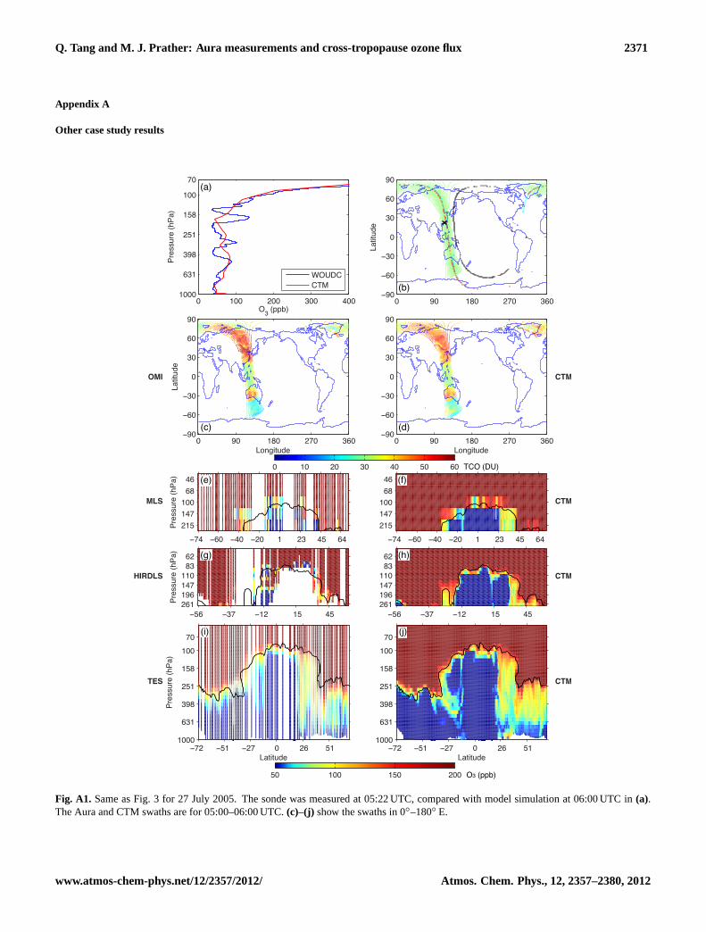
The other six cases (Figs.A1–A6) show very similar re-sults as the above two cases for different locations and time.In one case (Fig. A2, 6 July 2005) the CTM reproduces thelarge stratospheric fold at 200 hPa as seen by the sonde, andthe MLS and CTM patterns match quite well in Fig. A2e–f, except for the magnitudes of a few points. HIRDLS ob-serves a stratospheric intrusion at 45◦ N, 260–200 hPa, alsoin agreement with the model. In Fig. A4(3 August 2005)TES matches the CTM intrusion patterns at 25◦ S–10◦ S,630–160 hPa and at 40◦ N–50◦ N, 450–250 hPa. In Fig. A6(19 December 2005) TES and CTM agree on the intrusionpatterns at 20◦ N, 400–150 hPa as well as the high-O3 re-gion at 19◦ S–5◦ S, 630–400 hPa, although the TES pattern ismore spread out and lower in altitude.

Olsen et al.(2008) found a tropospheric intrusion withinthe stratosphere extending from the tropics to high latitudesin the HIRDLS data (v004) on 26 January 2006. Figure A7presents this case in the same way as the above eight casesexcept that there is no sonde available and the color scaleis adjusted to emphasize the stratospheric O3. In the newHIRDLS version (v5.00.00), the 2-km thick intrusion is alsofound near 110 hPa at 30◦ N–55◦ N (see Fig. A7g). Fig-ure A7h simulates this low O3 layer at the same location,but the O3 abundance in the surrounding air biases high rel-ative to the HIRDLS measurements due to known problemswith the stratospheric meteorology (Hsu and Prather, 2009).The MLS swath (Fig. A7e) indicates an inversion structureat 52◦ N, 100 hPa, which does not appear in the simulation(Fig. A7f).

These cases studies of the five Aura ozone measurementsand the CTM simulations, made on an instantaneous basis,confirm the model’s ability of reproducing the STE processesand show that the Aura measurements can detect some ofthe fine structures in O3, such as TFs and stratospheric in-trusions deep into the troposphere, while they miss a largenumber of such cases, presumably due to instrumental noise,lack of sensitivity, and vertical resolution in individual mea-surements. Like others, we find that the Aura measurementscan resolve stratosphere-troposphere folds for specific cases(Olsen et al., 2008; Manney et al., 2009; Pan et al., 2009;Manney et al., 2011). Combined with the 4-D hindcasts us-ing the CTM or with a data assimilation system, they maylead to a general, comprehensive integration of the globalSTE flux, but more work is needed.

6.2 CTM vs. Aura instantaneous comparisons

The observations of the three Aura ozone profilers –HIRDLS, MLS, and TES – do not coincide each other. Theydo not look at the same air mass at the same time and havedramatically different profiling techniques. From the pointof view of using the Aura observations to map out rapidly

www.atmos-chem-phys.net/12/2357/2012/ Atmos. Chem. Phys., 12, 2357–2380, 2012

2366 Q. Tang and M. J. Prather: Aura measurements and cross-tropopause ozone flux

0 200 400

0

200

400C

TM O

3 (ppb

)

NH Mid

246810

x 10−5

N=5858

−100 0 100 200−100

0

100

200

CTM

O3 (p

pb)

0.5

1

1.5

2x 10−4

N=5390

NH Jet

−100 0 100 200−100

0

100

200

CTM

O3 (p

pb)

Tropics

0.5

1

1.5

2x 10−4

N=15572

0 200 400

0

200

400

CTM

O3 (p

pb)

SH Jet

2

4

6

8

x 10−5

N=5625

0 200 400 600

0

200

400

600

MLS O3 (ppb)

CTM

O3 (p

pb)

SH Mid

0.5

1

1.5

2

x 10−5

N=5743

0 200 4000

100

200

300

400

500

246810

x 10−5

N=3297

0 100 2000

50

100

150

200

1

2

3x 10−4

N=2446

0 50 100 1500

50

100

150

N=2876

1

2

3

4x 10−4

0 200 4000

100

200

300

400

500

N=4169

24681012

x 10−5

0 200 400 6000

200

400

600

HIRDLS O3 (ppb)

N=6529

0.5

1

1.5

2x 10−5

0 200 4000

100

200

300

400

500

N=2249

2468101214

x 10−5

0 100 2000

50

100

150

200

N=1918

12345

x 10−4

0 50 100 1500

50

100

150

N=6944

2

4

6

8

x 10−4

0 200 4000

100

200

300

400

N=2309

0.511.522.5

x 10−4

0 200 4000

200

400

TES O3 (ppb)

N=2534

2

4

6

8x 10−5

0 200 400 6000

200

400

600

N=2249

5

10

15x 10−5

0 100 2000

50

100

150

200

1

2

3

4x 10−4

0 50 1000

50

100

246810

x 10−4

N=1918

N=6944

0 200 4000

100

200

300

400

0.5

1

1.5

2x 10−4

N=2309

0 200 400 600 8000

200

400

600

800

TES O3 (ppb)

1

2

3

4

x 10−5

N=2534

(a) (b) (c) (d)

(e) (f) (g) (h)

(i) (j) (k) (l)

(m) (n) (o) (p)

(q) (r) (s) (t)

Fig. 5. 2-D probability density functions (PDFs, unit: ppb−2) of CTM vs. Aura O3 for July 2005 at 215 hPa. Rows from top to bottomare for NH middle latitudes (40◦ N–50◦ N), NH jet (25◦ N–35◦ N), tropics (15◦ S–15◦ N), SH jet (35◦ S–25◦ S), and SH middle latitudes(50◦ S–40◦ S). Comparisons for different Aura ozone datasets are presented in columns from left to right: MLS, HIRDLS, and TES. TheCTM results processed with the TES operator are shown in the third column, and the raw model results in the fourth column. The 2-D PDFincludes all the good CTM-Aura pairs in the month and is weighted by the inverse of observation times for each latitude. It is normalized togive a 2-D integral of 1.N is the number of comparisons and the solid black line shows the 1:1 line. The mean biases and RMS are given inTable2.

changing tropopause folds and stratospheric intrusions, weneed a 4-D description of atmospheric O3 to determine ifthese instruments are measuring the same ozone. In this sec-tion, we use the UCI CTM as an intercomparison platformto study the consistency amongst the Aura ozone datasets fo-cusing on the UT/LS regions.

The 2-D probability density functions (PDFs) of the CTMvs. MLS, HIRDLS, and TES are shown for July 2005 andJanuary 2006 at 215 hPa and 147 hPa in Figs.5–8. ThesePDFs include every exact-match, CTM-Aura pair for five

latitude zones: NH middle latitude (40◦ N–50◦ N), NH jet(25◦ N–35◦ N), tropics (15◦ S–15◦ N), SH jet (35◦ S–25◦ S),and SH middle latitude (50◦ S–40◦ S). For TES, we presentthe comparisons for both the raw CTM simulation (fourthcolumn) and that convolved with the TES operator (third col-umn). The PDF (unit of frequency per ppb2) is weighted in-versely by the sampling times for each latitude to account forunequal observations from different latitudes, and it is nor-malized to give an integral of 1. The number of CTM-Auraexact matches for the month are shown on each panel.

Atmos. Chem. Phys., 12, 2357–2380, 2012 www.atmos-chem-phys.net/12/2357/2012/

Q. Tang and M. J. Prather: Aura measurements and cross-tropopause ozone flux 2367

Table 2. Mean biases and RMS errors (unit: ppb) of CTM versus MLS, HIRDLS, and TES for five regions at 215 hPa and 147 hPa for July2005a.

MLS HIRDLS TES TES*

Regions 215 hPa 147 hPa 215 hPa 147 hPa 215 hPa 147 hPa 215 hPa 147 hPa

NH Mid-L 10.0±79.2 51.6±125.6 −48.1±186.7 34.8±144.1 7.9±42.1 23.7±75.8 −22.2±79.8 −5.1±154.0NH Jet 7.0±57.0 11.7±135.6 −15.1±60.9 −32.6±157.5 5.1±25.0 11.1±53.8 −2.8±34.1 −5.3±105.9Tropics 8.6±45.3 −12.2±151.8 −6.6±34.5 −63.3±183.2 11.7±17.7 21.0±41.3 2.5±17.8 −5.3±85.6SH Jet 42.3±80.0 150.7±162.1 58.4±109.6 136.0±174.9 72.6±69.7 129.6±113.7 34.8±84.1 133.6±159.3SH Mid-L 43.7±106.8 386.9±301.7 96.2±229.7 393.3±343.8 77.5±71.8 225.1±196.5 90.8±131.9 328.1±294.2

aThe latitude ranges are NH middle latitude (40◦ N–50◦ N), NH jet (25◦ N–35◦ N), tropics (15◦ S–15◦ N), SH jet (35◦ S–25◦ S), and SH middle latitude (50◦ S–40◦ S). The resultsare shown in the format of the mean bias±RMS and defined as the CTM less Aura. The number of comparisons (N) is shown in Figs.5 and6 and the SEM values are generallyabout 1 ppb and less than 3 ppb. TES* denotes the comparisons with the raw CTM outputs.

CTM

O3 (p

pb)

NH Mid

CTM

O3 (p

pb)

NH Jet

CTM

O3 (p

pb)

Tropics

CTM

O3 (p

pb)

SH Jet

CTM

O3 (p

pb)

SH Mid

0 200 400 600 8000

200

400

600

800

N=5858

12345

x 10−5

0 100 200 300

0

100

200

300

2468101214

x 10−5

−100 0 100 200−100

0

100

200

5

10

15

x 10−5

0 200 400 600 8000

200

400

600

800

1

2

3

4x 10−5

0 500 10000

500

1000

MLS O3 (ppb)

5

10

15x 10−6

0 200 400 600 8000

200

400

600

800

N=6574

2

4

6x 10−5

N=5390

N=15572

N=5625

N=5743

0 200 4000

100

200

300

400

N=3762

24681012

x 10−5

0 200 4000

100

200

300

400

N=5002

2468101214

x 10−5

0 200 400 600 8000

200

400

600

800

N=6156

1

2

3

4x 10−5

0 500 10000

500

1000

HIRDLS O3 (ppb)

N=9507

5

10

15x 10−6

0 200 400 600 8000

200

400

600

800

N=2249

2

4

6x 10−5

0 200 4000

100

200

300

400

N=1918

0.511.522.5

x 10−4

0 100 2000

50

100

150

200

N=6944

1

2

3

4x 10−4

0 200 400 600 8000

200

400

600

800

N=2309

246810

x 10−5

0 500 10000

500

1000

TES O3 (ppb)

N=2534

0.511.522.5

x 10−5

0 200 400 600 8000

200

400

600

800

N=2249

2

4

6

8x 10−5

0 200 4000

100

200

300

400

N=1918

0.5

1

1.5

x 10−4

0 100 2000

50

100

150

200

N=6944

1

2

3

4

x 10−4

0 200 400 600 8000

200

400

600

800

N=2309

2

4

6

x 10−5

0 500 1000 15000

500

1000

1500

TES O3 (ppb)

N=2534

0.5

1

1.5

2

x 10−5

(a) (b) (c) (d)

(e) (f) (g) (h)

(i) (j) (k) (l)

(m) (n) (o) (p)

(q) (r) (s) (t)

Fig. 6. Same as Fig.5 for July 2005 at 147 hPa.

www.atmos-chem-phys.net/12/2357/2012/ Atmos. Chem. Phys., 12, 2357–2380, 2012

2368 Q. Tang and M. J. Prather: Aura measurements and cross-tropopause ozone flux

CTM

O3 (p

pb)

NH Mid

CTM

O3 (p

pb)

NH Jet

CTM

O3 (p

pb)

Tropics

CTM

O3 (p

pb)

SH Jet

CTM

O3 (p

pb)

SH Mid

0 200 400 600 800

0

200

400

600

800

N=6060

5

10

15

x 10−6

0 200 400−100

0

100

200

300

400

N=6050

246810

x 10−5

−100 0 100 200−100

0

100

200

N=16149

0.5

1

1.5

2

x 10−4

−100 0 100 200−100

0

100

200

N=6038

5

10

15

x 10−5

0 200 400 600

0

200

400

600

MLS O3 (ppb)

N=6233

2

4

6

8

x 10−5

0 200 400 600 8000

200

400

600

800

N=5896

0.5

1

1.5

2x 10−5

0 200 4000

100

200

300

400

N=4187

5

10

15

x 10−5

0 50 100 1500

50

100

150

N=2918

2

4

6

x 10−4

0 100 2000

50

100

150

200

250

N=3264

0.5

1

1.5

2x 10−4

0 200 400 6000

200

400

600

HIRDLS O3 (ppb)

N=5809

2

4

6

8x 10−5

0 200 400 600 8000

200

400

600

800

N=2448

12345

x 10−5

0 100 200 3000

100

200

300

N=2169

0.511.522.5

x 10−4

0 50 1000

50

100

N=6904

246810

x 10−4

0 100 2000

50

100

150

200

N=2207

1

2

3

4x 10−4

0 200 4000

100

200

300

400

500

TES O3 (ppb)

N=2517

5

10

15

x 10−5

0 500 10000

500

1000

N=2448

1

2

3

4

x 10−5

0 200 4000

100

200

300

400

500

N=2169

0.511.522.5

x 10−4

0 50 1000

50

100

N=6904

2

4

6

8x 10−4

0 100 2000

50

100

150

200

250

N=2207

1

2

3

x 10−4

0 200 400 6000

200

400

600

TES O3 (ppb)

N=2517

5

10

15

x 10−5

(a) (b) (c) (d)

(e) (f) (g) (h)

(i) (j) (k) (l)

(m) (n) (o) (p)

(q) (r) (s) (t)

Fig. 7. Same as Fig.5 for January 2006 at 215 hPa. The mean biases and RMS are given in Table3.

Table 3. Same as Table2 for January 2006a.

MLS HIRDLS TES TES*

Regions 215 hPa 147 hPa 215 hPa 147 hPa 215 hPa 147 hPa 215 hPa 147 hPa

NH Mid-L 61.4±121.2 344.1±257.7 105.9±823.9 344.8±288.2 73.9±67.3 155.3±111.4 94.4±129.9 331.6±297.7NH Jet 37.0±77.0 61.4±209.8 52.3±94.4 56.0±174.6 30.7±39.6 44.6±94.6 33.8±86.1 53.1±180.3Tropics 11.0±66.4 −13.2±242.5 5.2±74.4 −26.2±212.3 8.4±40.4 14.7±107.0 7.1±68.2 1.5±167.4SH Jet 5.8±70.9 37.3±201.0 11.8±76.9 13.0±187.0 22.6±33.9 61.7±76.4 1.0±81.9 5.1±178.9SH Mid-L 49.4±79.3 188.4±150.6 87.9±138.7 210.7±165.4 54.7±45.9 148.9±106.0 37.9±96.9 92.7±155.6

a The number of comparisons (N) is shown in Figs.7 and8.

Atmos. Chem. Phys., 12, 2357–2380, 2012 www.atmos-chem-phys.net/12/2357/2012/

Q. Tang and M. J. Prather: Aura measurements and cross-tropopause ozone flux 2369

CTM

O3 (p

pb)

NH Mid

CTM

O3 (p

pb)

NH Jet

CTM

O3 (p

pb)

Tropics

CTM

O3 (p

pb)

SH Jet

CTM

O3 (p

pb)

SH Mid

0 500 1000 15000

500

1000

1500

N=6060

2

4

6

8

10

x 10−6

0 200 400

0

200

400

N=6050

2

4

6

x 10−5

−100 0 100 200−100

0

100

200

N=16149

0.5

1

1.5

2

x 10−4

0 200 400−100

0

100

200

300

400

N=6038

246810

x 10−5

0 200 400 600 8000

200

400

600

800

MLS O3 (ppb)

N=6233

0.5

1

1.5

2

2.5x 10−5

0 1000 20000

500

1000

1500

2000

N=8127

2

4

6

8

10x 10−6

0 200 400 6000

200

400

600

N=7472

2

4

6

x 10−5

0 100 2000

50

100

150

200

250

N=4430

0.511.522.5

x 10−4

0 200 4000

100

200

300

400

N=5927

2

4

6

8

x 10−5

0 500 10000

500

1000

HIRDLS O3 (ppb)

N=10004

0.5

1

1.5

2

x 10−5

0 500 1000 15000

500

1000

1500

N=2448

1

2

3x 10−5

0 200 4000

100

200

300

400

500

N=2169

24681012

x 10−5

0 50 100 1500

50

100

150

N=6904

2

4

6

x 10−4

0 200 4000

100

200

300

400

N=2207

2468101214

x 10−5

0 500 10000

500

1000

TES O3 (ppb)

N=2517

12345

x 10−5

0 1000 20000

500

1000

1500

2000

N=2448

0.5

1

1.5

2x 10−5

0 200 4000

100

200

300

400

500

N=2169

246810

x 10−5

0 50 100 1500

50

100

150

N=6904

2

4

6

x 10−4

0 200 4000

100

200

300

400

500

N=2207

24681012

x 10−5

0 500 10000

500

1000

TES O3 (ppb)

N=2517

12345

x 10−5

(a) (b) (c) (d)

(e) (f) (g) (h)

(i) (j) (k) (l)

(m) (n) (o) (p)

(q) (r) (s) (t)

Fig. 8. Same as Fig.5 for January 2006 at 147 hPa. The mean biases and RMS are given in Table3.

The red, high-density pixels are generally located close tothe black solid, 1:1 line for all the three instruments, indicat-ing small biases, except for stratospheric comparisons suchas Fig.6q–t. The CTM is generally biased high compared toall three Aura measurements in the lower stratosphere, sug-gesting a model deficiency that is most likely due to the errorsin the stratospheric circulation of the 40-layer ECMWF me-teorological fields previously noted (Hsu and Prather, 2009).As expected, TES gives generally tighter PDFs than MLSand HIRDLS, reflecting the differences between nadir andlimb scanning. For tropospheric model values (<100 ppb),such as in the tropics and jet regions of the summer hemi-sphere (Fig.5e, f, i, j), the slopes of MLS and HIRDLS PDFare almost flat, consistent with low sensitivities and noise inthe lowermost layers of these limb scanning measurements.Negative MLS profile values (e.g., Fig.5a, q) are allowed in

the retrieval algorithm to achieve the correct column load-ing (Livesey et al., 2007). The PDFs of HIRDLS are no-tably more dispersed compared to those of MLS and TES at215 hPa for the winter hemisphere middle latitudes (Fig.5rand Fig.7b), indicating greater noise in the HIRDLS mea-surements for this region and season. With the TES opera-tor, the tropospheric CTM values (<100 ppb) become strato-spheric (>100 ppb) (e.g., Fig.5c–d and Fig.7s–t) as previ-ously shown in Sect.4.6. The CTM-TES comparisons areusually improved with application of the TES operator (e.g.,Fig.5g–h and Fig.8g–h) due to the relaxing towards the TESa priori and reducing the variance at a given pressure level byvertical smoothing (see Tables2 and3). Without some clearindication of the relative influence of the a prior in each re-trieval, this CTM-TES agreement may be artificial.

www.atmos-chem-phys.net/12/2357/2012/ Atmos. Chem. Phys., 12, 2357–2380, 2012

2370 Q. Tang and M. J. Prather: Aura measurements and cross-tropopause ozone flux

Tables2 and3 summarize the mean biases and root meansquare (RMS) errors for Figs.5–8. The RMS errors are gen-erally much larger than the biases, consistent with previousvalidations against ozone sondes (Jiang et al., 2007; Nassaret al., 2008; Zhang et al., 2010), and are most likely due to thehigh variability at this pressure range for all latitude zonesin both summer and winter. Note that the biases are lessmeaningful given such large RMS, and thus are only goodfor qualitative, long-term averages (i.e., L3 monthly griddeddata). The biases clearly show that the CTM overestimatesin subtropical jet and mid-latitude regions, again recognizingthe model deficiency in these regions.

The results in Tables2 and 3 identify inconsistenciesamong the Aura datasets. In July 2005 at 215 hPa, the CTMmeans are smaller than MLS and TES, while greater thanHIRDLS in the tropics, NH jets, and mid-latitudes. Com-pared with sondes, TES has at most a 15 % high bias in thetroposphere (Nassar et al., 2008; Richards et al., 2008), whileMLS has a∼20 % high bias at the middle to high-latitudestropopause (Jiang et al., 2007). We have now shown thatHIRDLS has large positive biases of∼30–100 ppb at 215 hPafrom the tropics to NH mid-latitudes in summer. In the trop-ics at 147 hPa, the CTM is smaller than MLS and HIRDLSbut larger than TES for both July 2005 and January 2006,identifying a clear discrepancy between MLS-HIRDLS andTES without having to find collocated observations. In thiscase the RMS is much larger than the mean biases althoughthe standard error of the mean (SEM) calculated assuming anormal distribution is smaller. The bias does not show in in-dividual measurements, and the statistical significance of thebias in L3 gridded data depends greatly on the assumption ofa normally distributed error that does not depend systemati-cally on specific atmospheric conditions.

7 Conclusions

The high-resolution CTM (1◦ ×1◦×40-layer× 0.5 h) simu-

lation of ozone reveals that the time scale of stratosphere-troposphere exchange (STE) processes observed at a givenlocation is as short as hours and indicates that STE occurson a spatial scale of a few hundred kilometers. For nadir-view instruments (e.g., OMI and TES), the application oftheir satellite operators (averaging kernel (AK) and a priori)can cause artificially high bias in the upper troposphere, asthe nadir-view measurements have coarse vertical resolutionsand their AK can smear the high O3 abundances in the strato-sphere into the troposphere.

Aura without a fully functioning HIRDLS is not well de-signed for studying STE. The L2 swath data from Aura arechosen to study the STE flux of ozone based upon the short-lived features of most STE processes and previous case stud-ies (Olsen et al., 2008; Manney et al., 2009; Pan et al., 2009;Manney et al., 2011). The high-resolution simulation withthe UCI CTM depicts the full ozone picture for years 2005–2006 to compare with the individual, mostly non-coincidentAura ozone measurements derived from different remotesensing techniques. The model’s ability to reproduce STE-related processes, such as tropospheric folds (TFs), is con-firmed by the comparisons with the WOUDC sondes, givingconfidence on the reliability and accuracy of the folding andintrusion structures simulated along Aura swaths.

From the eight case studies here, the four Aura instrumentsdemonstrate some skill in catching the STE structures, ei-ther from the high TCO anomalies (for OMI) or from theO3 vertical profiles (for HIRDLS, MLS, and TES). Never-theless, many of the features simulated by the model are notseen in the L2 data. Tropopause folds and stratospheric in-trusions of O3 present a fundamental difficulty for satellitepassive remote sensing due to large abundances and columnsof stratospheric ozone above the troposphere. Beyond thiswork, Aura datasets have been studied for only a few STEcases, such asPan et al.(2009); Manney et al.(2011). Im-provements in the instruments and sensing techniques so asto greatly reduce the apparent noise in individual retrievalswill be necessary if satellite observations are to be used tomap out folds and intrusions on a regular basis and thus pro-vide better constraint for the STE modeling.

We use the CTM as an intercomparison platform to inves-tigate the consistency of different Aura ozone measurementsthat are close but not coincident in space, time, or averag-ing kernel. The CTM deficiencies can be readily identifiedwhen the biases are similar against all Aura observations.The 2-D PDF as well as the mean biases and RMS of exactlymatched CTM-Aura data identifies the model’s high biasesin the lower stratosphere. On the other hand, the CTM asa transfer standard can be used to identify clearly the rela-tive biases in the Aura ozone instruments on an instantaneousbasis, including the meteorology at the time of observation,even when they do not have overlapping measurements. Forexample, the case study for July 2005 (Table2) quantifies thedifferent model-measurement biases for HIRDLS, MLS, andTES in the UT/LS region, thus identifying both consistenciesand inconsistencies across these Aura datasets.

Atmos. Chem. Phys., 12, 2357–2380, 2012 www.atmos-chem-phys.net/12/2357/2012/

Q. Tang and M. J. Prather: Aura measurements and cross-tropopause ozone flux 2371

Appendix A

Other case study results

0 100 200 300 400

70

100

158

251

398

631

1000

O3 (ppb)

Pres

sure

(hPa

)

WOUDCCTM

0 90 180 270 360−90

−60

−30

0

30

60

90

Latit

ude

0 90 180 270 360−90

−60

−30

0

30

60

90

Longitude

Latit

ude

0 90 180 270 360−90

−60

−30

0

30

60

90

Longitude

0 10 20 30 40 50 60

−74 −60 −40 −20 1 23 45 64215147100 68 46

Pres

sure

(hPa

)

−74 −60 −40 −20 1 23 45 64215147100 68 46

−56 −37 −12 15 45261196147110 83 62

Pres

sure

(hPa

)

−56 −37 −12 15 45261196147110 83 62

−72 −51 −27 0 26 51

70100

158

251

398

631

1000

Latitude

Pres

sure

(hPa

)

−72 −51 −27 0 26 51

70100

158

251

398

631

1000

Latitude

50 100 150 200

(i) (j)

TCO (DU)(e) (f)

(g) (h)

O3 (ppb)

(a)

(b)

(c) (d)

OMI CTM

MLS CTM

TES

CTMHIRDLS

CTM

Fig. A1. Same as Fig.3 for 27 July 2005. The sonde was measured at 05:22 UTC, compared with model simulation at 06:00 UTC in(a).The Aura and CTM swaths are for 05:00–06:00 UTC.(c)–(j) show the swaths in 0◦–180◦ E.

www.atmos-chem-phys.net/12/2357/2012/ Atmos. Chem. Phys., 12, 2357–2380, 2012

2372 Q. Tang and M. J. Prather: Aura measurements and cross-tropopause ozone flux

0 100 200 300 400

70

100

158

251

398

631

1000

O3 (ppb)

Pres

sure

(hPa

)

WOUDCCTM

0 90 180 270 360−90

−60

−30

0

30

60

90

Latit

ude

0 90 180 270 360−90

−60

−30

0

30

60

90

Longitude

Latit

ude

0 90 180 270 360−90

−60

−30

0

30

60

90

Longitude

0 10 20 30 40 50 60

2 25 46 65215147100 68 46

Pres

sure

(hPa

)

2 25 46 65215147100 68 46

−34 −10 16 45261196147110 83 62

Pres

sure

(hPa

)

−34 −10 16 45261196147110 83 62

−21 −8 4 17 29 41 55 65

70100

158

251

398

631

1000

Latitude

Pres

sure

(hPa

)

−21 −8 4 17 29 41 55 65

70100

158

251

398

631

1000

Latitude

50 100 150 200

(i) (j)

TCO (DU)(e) (f)

(g) (h)

O3 (ppb)

(a)

(b)

(c) (d)

OMI CTM

MLS CTM

TES

CTMHIRDLS

CTM

Fig. A2. Same as Fig.3 for 6 July 2005. The sonde is from Ankara (40.0◦ N, 32.9◦ E, station code 348) at 11:52 UTC, compared with modelsimulation at 12:00 UTC in(a). The Aura and CTM swaths are for 10:00–11:00 UTC.(c)–(j) show the swaths in 0◦–134◦ E.

Atmos. Chem. Phys., 12, 2357–2380, 2012 www.atmos-chem-phys.net/12/2357/2012/

Q. Tang and M. J. Prather: Aura measurements and cross-tropopause ozone flux 2373

0 100 200 300 400

70

100

158

251

398

631

1000

O3 (ppb)

Pres

sure

(hPa

)

WOUDCCTM

0 90 180 270 360−90

−60

−30

0

30

60

90

Latit

ude

0 90 180 270 360−90

−60

−30

0

30

60

90

Longitude

Latit

ude

0 90 180 270 360−90

−60

−30

0

30

60

90

Longitude

0 10 20 30 40 50 60

−40 −17 4 26 48 67215147100 68 46

Pres

sure

(hPa

)

−40 −17 4 26 48 67215147100 68 46

−52 −33 −10 17 46261196147110 83 62

Pres

sure

(hPa

)

−52 −33 −10 17 46261196147110 83 62

−65 −42 −15 10 38 62

70100

158

251

398

631

1000

Latitude

Pres

sure

(hPa

)

−65 −42 −15 10 38 62

70100

158

251

398

631

1000

Latitude

50 100 150 200

(i) (j)

TCO (DU)(e) (f)

(g) (h)

O3 (ppb)

(a)

(b)

(c) (d)

OMI CTM

MLS CTM

TES

CTMHIRDLS

CTM

Fig. A3. Same as Fig. A2for 20 July 2005. The sonde was measured at 11:37 UTC, compared with model simulation at 12:00 UTC in(a).The Aura and CTM swaths are for 10:00–11:00 UTC.(c)–(j) show the swaths in 0◦–99◦ E.

www.atmos-chem-phys.net/12/2357/2012/ Atmos. Chem. Phys., 12, 2357–2380, 2012

2374 Q. Tang and M. J. Prather: Aura measurements and cross-tropopause ozone flux

0 100 200 300 400

70

100

158

251

398

631

1000

O3 (ppb)

Pres

sure

(hPa

)

WOUDCCTM

0 90 180 270 360−90

−60

−30

0

30

60

90

Latit

ude

0 90 180 270 360−90

−60

−30

0

30

60

90

Longitude

Latit

ude

0 90 180 270 360−90

−60

−30

0

30

60

90

Longitude

0 10 20 30 40 50 60

−73 −56 −38 −17 6 29 50 68215147100 68 46

Pres

sure

(hPa

)

−73 −56 −38 −17 6 29 50 68215147100 68 46

−53 −36 −12 14 43261196147110 83 62

Pres

sure

(hPa

)

−53 −36 −12 14 43261196147110 83 62

−71 −48 −23 2 29 53

70100

158

251

398

631

1000

Latitude

Pres

sure

(hPa

)

−71 −48 −23 2 29 53

70100

158

251

398

631

1000

Latitude

50 100 150 200

(i) (j)

TCO (DU)(e) (f)

(g) (h)

O3 (ppb)

(a)

(b)

(c) (d)

OMI CTM

MLS CTM

TES

CTMHIRDLS

CTM

Fig. A4. Same as Fig. A2for 3 August 2005. The sonde was measured at 11:36 UTC.

Atmos. Chem. Phys., 12, 2357–2380, 2012 www.atmos-chem-phys.net/12/2357/2012/

Q. Tang and M. J. Prather: Aura measurements and cross-tropopause ozone flux 2375

0 100 200 300 400

70

100

158

251

398

631

1000

O3 (ppb)

Pres

sure

(hPa

)

WOUDCCTM

0 90 180 270 360−90

−60

−30

0

30

60

90

Latit

ude

0 90 180 270 360−90

−60

−30

0

30

60

90

Longitude

Latit

ude

0 90 180 270 360−90

−60

−30

0

30

60

90

Longitude

0 10 20 30 40 50 60

5 27 48 68215147100 68 46

Pres

sure

(hPa

)

5 27 48 68215147100 68 46

−32 −6 21 50261196147110 83 62

Pres

sure

(hPa

)

−32 −6 21 50261196147110 83 62

−18 −4 8 21 35 50 61 71

70100

158

251

398

631

1000

Latitude

Pres

sure

(hPa

)

−18 −4 8 21 35 50 61 71

70100

158

251

398

631

1000

Latitude

50 100 150 200

(i) (j)

TCO (DU)(e) (f)

(g) (h)

O3 (ppb)

(a)

(b)

(c) (d)

OMI CTM

MLS CTM

TES

CTMHIRDLS

CTM

Fig. A5. Same as Fig.3 for 2 February 2005. The sonde is from Maxaranguape (5.4◦ S, 35.4◦ W, station code 466) at 15:45 UTC, comparedwith model simulation at 16:00 UTC in(a). The Aura and CTM swaths are for 16:00–17:00 UTC.(c)–(j) show the swaths in 251◦ E–360◦ E.

www.atmos-chem-phys.net/12/2357/2012/ Atmos. Chem. Phys., 12, 2357–2380, 2012

2376 Q. Tang and M. J. Prather: Aura measurements and cross-tropopause ozone flux

0 100 200 300 400

70

100

158

251

398

631

1000

O3 (ppb)

Pres

sure

(hPa

)

WOUDCCTM

0 90 180 270 360−90

−60

−30

0

30

60

90

Latit

ude

0 90 180 270 360−90

−60

−30

0

30

60

90

Longitude

Latit

ude

0 90 180 270 360−90

−60

−30

0

30

60

90

Longitude

0 10 20 30 40 50 60

8 31 52 69215147100 68 46

Pres

sure

(hPa

)

8 31 52 69215147100 68 46

−32 −4 22 51261196147110 83 62

Pres

sure

(hPa

)

−32 −4 22 51261196147110 83 62

−19 −5 7 20 32 46 57 67

70100

158

251

398

631

1000

Latitude

Pres

sure

(hPa

)

−19 −5 7 20 32 46 57 67

70100

158

251

398

631

1000

Latitude

50 100 150 200

(i) (j)

TCO (DU)(e) (f)

(g) (h)

O3 (ppb)

(a)

(b)

(c) (d)

OMI CTM

MLS CTM

TES

CTMHIRDLS

CTM

Fig. A6. Same as Fig. A5 for 19 December 2005. The sonde was measured at 16:00 UTC.

Atmos. Chem. Phys., 12, 2357–2380, 2012 www.atmos-chem-phys.net/12/2357/2012/

Q. Tang and M. J. Prather: Aura measurements and cross-tropopause ozone flux 2377

0 90 180 270 360−90

−60

−30

0

30

60

90

Latit

ude

Longitude Longitude

0 10 20 30 40 50 60

0 90 180 270 360−90

−60

−30

0

30

60

90

Latit

ude

0 90 180 270 360−90

−60

−30

0

30

60

90

11 32 52 71 78215147100 68 46

Pres

sure

(hPa

)

11 32 52 71 78215147100 68 46

19 34 48 61 71261196147110 83 62

Pres

sure

(hPa

)

19 34 48 61 71261196147110 83 62

−13 0 13 26 39 53 65 73

70100

158

251

398

631

1000

Latitude

Pres

sure

(hPa

)

−13 0 13 26 39 53 65 73

70100

158

251

398

631

1000

Latitude

0 1 2 3 4 5

(i) (j)

TCO (DU)(e) (f)

(g) (h)

O3 (ppm)

(b)

(c) (d)

OMI CTM

MLS CTM

TES

CTMHIRDLS

CTM

Fig. A7. Same as Fig.3 for 26 January 2006 except that no sonde is available and the e90 tropopause is indicated by red solid lines in(e)–(j) .The Aura and CTM swaths are for 22:00–23:00 UTC.(c)–(j) show the swaths in 181◦ E–270◦ E. (g) and(h) only show the HIRDLS swathat 19◦ N–74◦ N to mimic the Fig. 1 ofOlsen et al.(2008).

www.atmos-chem-phys.net/12/2357/2012/ Atmos. Chem. Phys., 12, 2357–2380, 2012

2378 Q. Tang and M. J. Prather: Aura measurements and cross-tropopause ozone flux

Acknowledgements.The authors thank Anne Douglass and anony-mous reviewers for their careful, detailed review and constructivesuggestions. This work is funded by NASA grant (NNX08AR25G)to UCI and NSF grant (AGS-1042787) to Cornell University.

Edited by: D. Shindell

References

Alexander, M. J., Gille, J., Cavanaugh, C., Coffey, M., Craig, C.,Eden, T., Francis, G., Halvorson, C., Hannigan, J., Khosravi,R., Kinnison, D., Lee, H., Massie, S., Nardi, B., Barnett, J.,Hepplewhite, C., Lambert, A., and Dean, V.: Global estimatesof gravity wave momentum flux from High Resolution Dynam-ics Limb Sounder observations, J. Geophys. Res., 113, D15S18,doi:10.1029/2007JD008807, 2008.

Atkinson, R. and Arey, J.: Gas-phase tropospheric chemistry of bio-genic volatile organic compounds: a review, Atmos. Environ.,37, 197–219,doi:10.1016/S1352-2310(03)00391-1, 2003.

Carver, G., Brown, P., and Wild, O.: The ASAD atmospheric chem-istry integration package and chemical reaction database, Com-put. Phys. Commun., 105, 197–215, 1997.

Danielsen, E. F.: Stratospheric-tropospheric exchange based on ra-dioactivity, ozone and potential vorticity, J. Atmos. Sci., 25, 502–518, 1968.

de Haan, J. F. and Veefkind, J. P.: OMO3PR Readme,http://disc.sci.gsfc.nasa.gov/Aura/data-holdings/OMI/documents/v003/OMO3PROREADME.html, 2009.

Denman, K. L., Brasseur, G., Chidthaisong, A., Ciais, P., Cox,P. M., Dickinson, R. E., Hauglustaine, D., Heinze, C., Holland,E., Jacob, D., Lohmann, U., Ramachandran, S., da Silva Dias,P. L., Wofsy, S. C., and Zhang, X.: Couplings Between Changesin the Climate System and Biogeochemistry, in: Climate Change2007: The Physical Science Basis. Contribution of WorkingGroup I to the Fourth Assessment Report of the Intergovernmen-tal Panel on Climate Change, edited by Solomon, S., Qin, D.,Manning, M., Chen, Z., Marquis, M., Averyt, K. B., Tignor, M.,and Miller, H. L., chap. 7, pp. 499–587, Cambridge UniversityPress, Cambridge, United Kingdom and New York, NY, USA,2007.

Fusco, A. C. and Logan, J. A.: Analysis of 1970–1995 trendsin tropospheric ozone at Northern Hemisphere midlatitudeswith the GEOS-CHEM model, J. Geophys. Res., 108, 4449,doi:10.1029/2002JD002742, 2003.

Gauss, M., Myhre, G., Isaksen, I. S. A., Grewe, V., Pitari, G., Wild,O., Collins, W. J., Dentener, F. J., Ellingsen, K., Gohar, L. K.,Hauglustaine, D. A., Iachetti, D., Lamarque, F., Mancini, E.,Mickley, L. J., Prather, M. J., Pyle, J. A., Sanderson, M. G.,Shine, K. P., Stevenson, D. S., Sudo, K., Szopa, S., and Zeng, G.:Radiative forcing since preindustrial times due to ozone changein the troposphere and the lower stratosphere, Atmos. Chem.Phys., 6, 575–599,doi:10.5194/acp-6-575-2006, 2006.

Gettelman, A., Holton, J. R., and Rosenlof, K. H.: Mass fluxes ofO3, CH4, N2O and CF2Cl2 in the lower stratosphere calculatedfrom observational data, J. Geophys. Res., 102, 19149–19159,doi:10.1029/97JD01014, 1997.

HIRDLS Team: High Resolution Dynamics Limb SounderEarth Observing System (EOS) Data Description and Qual-

ity Version 5 (V5), http://disc.sci.gsfc.nasa.gov/Aura/data-holdings/HIRDLS/documents/HIRDLS-V5-DQD-6May2010.pdf, last access: 10 May 2010, 2010.

Holmes, C. D., Tang, Q., and Prather, M. J.: Uncertainties in cli-mate assessment for the case of aviation NO, P. Natl. Acad.Sci. U.S.A., 108, 10 997–11 002,doi:10.1073/pnas.1101458108,2011.

Hoor, P., Borken-Kleefeld, J., Caro, D., Dessens, O., Endresen,O., Gauss, M., Grewe, V., Hauglustaine, D., Isaksen, I. S. A.,Jockel, P., Lelieveld, J., Myhre, G., Meijer, E., Olivie, D.,Prather, M., Schnadt Poberaj, C., Shine, K. P., Staehelin, J.,Tang, Q., van Aardenne, J., van Velthoven, P., and Sausen, R.:The impact of traffic emissions on atmospheric ozone and OH:results from QUANTIFY, Atmos. Chem. Phys., 9, 3113–3136,doi:10.5194/acp-9-3113-2009, 2009.

Hsu, J. and Prather, M. J.: Stratospheric variability andtropospheric ozone, J. Geophys. Res., 114, D06102,doi:10.1029/2008JD010942, 2009.

Hsu, J., Prather, M. J., and Wild, O.: Diagnosing the stratosphere-to-troposphere flux of ozone in a chemistry transport model, J.Geophys. Res., 110, D19305,doi:10.1029/2005JD006045, 2005.

Isaksen, I. S. A., Zerefos, C., Kourtidis, K., Meleti, C., Dalsoren,S. B., Sundet, J. K., Grini, A., Zanis, P., and Balis, D.: Tro-pospheric ozone changes at unpolluted and semipolluted regionsinduced by stratospheric ozone changes, J. Geophys. Res., 110,D02302,doi:10.1029/2004JD004618, 2005.

Jiang, Y. B., Froidevaux, L., Lambert, A., Livesey, N. J., Read,W. G., Waters, J. W., Bojkov, B., Leblanc, T., McDermid, I. S.,Godin-Beekmann, S., Filipiak, M. J., Harwood, R. S., Fuller,R. A., Daffer, W. H., Drouin, B. J., Cofield, R. E., Cuddy, D. T.,Jarnot, R. F., Knosp, B. W., Perun, V. S., Schwartz, M. J., Snyder,W. V., Stek, P. C., Thurstans, R. P., Wagner, P. A., Allaart, M.,Andersen, S. B., Bodeker, G., Calpini, B., Claude, H., Coetzee,G., Davies, J., Backer, H. D., Dier, H., Fujiwara, M., Johnson,B., Kelder, H., Leme, N. P., Konig-Langlo, G., Kyro, E., Lan-eve, G., Fook, L. S., Merrill, J., Morris, G., Newchurch, M.,Oltmans, S., Parrondos, M. C., Posny, F., Schmidlin, F., Skri-vankova, P., Stubi, R., Tarasick, D., Thompson, A., Thouret,V., Viatte, P., Vomel, H., von Der Gathen, P., Yela, M., andZablocki, G.: Validation of Aura Microwave Limb SounderOzone by ozonesonde and lidar measurements, J. Geophys. Res.,112, D24S34,doi:10.1029/2007JD008776, 2007.

Kraabøl, A. G., Berntsen, T. K., Sundet, J. K., and Stordal,F.: Impacts of NOx emissions from subsonic aircraft ina global three-dimensional chemistry transport model in-cluding plume processes, J. Geophys. Res., 107, 4655,doi:10.1029/2001JD001019, 2002.

Lacis, A. A., Wuebbles, D. J., and Logan, J. A.: Radiative Forcingof Climate by Changes in the Vertical Distribution of Ozone, J.Geophys. Res., 95, 9971–9981,doi:10.1029/JD095iD07p09971,1990.

Livesey, N. J., Read, W. G., Lambert, A., Cofield, R. E., Cuddy,D. T., Froidevaux, L., Fuller, R. A., Jarnot, R. F., Jiang, J. H.,Jiang, Y. B., Knosp, B. W., Kovalenko, L. J., Pickett, H. M.,Pumphrey, H. C., Santee, M. L., Schwartz, M. J., Stek, P. C.,Wagner, P. A., Waters, J. W., and Wu, D. L.: Earth ObservingSystem (EOS) Aura Microwave Limb Sounder (MLS) Version2.2 Level 2 data quality and description document, Tech. Rep.D-33509, JPL, Jet Propulsion Laboratory California Institute of

Atmos. Chem. Phys., 12, 2357–2380, 2012 www.atmos-chem-phys.net/12/2357/2012/

Q. Tang and M. J. Prather: Aura measurements and cross-tropopause ozone flux 2379

Technology Pasadena, California, 91109–8099, 2007.Livesey, N. J., Read, W. G., Froidevaux, L., Lambert, A., Man-

ney, G. L., Pumphrey, H. C., Santee, M. L., Schwartz, M. J.,Wang, S., Cofield, R. E., Cuddy, D. T., Fuller, R. A., Jarnot, R. F.,Jiang, J. H., Knosp, B. W., Stek, P. C., Wagner, P. A., and Wu,D. L.: Earth Observing System (EOS) Aura Microwave LimbSounder (MLS) Version 3.3 Level 2 data quality and descriptiondocument, Tech. Rep. D-33509, JPL, Jet Propulsion LaboratoryCalifornia Institute of Technology Pasadena, California, 91109–8099, 2011.

Luo, M., Rinsland, C., Fisher, B., Sachse, G., Diskin, G., Logan, J.,Worden, H., Kulawik, S., Osterman, G., Eldering, A., Herman,R., and Shephard, M.: TES carbon monoxide validation withDACOM aircraft measurements during INTEX-B 2006, J. Geo-phys. Res., 112, D24S48,doi:10.1029/2007JD008803, 2007.

Manney, G. L., Harwood, R. S., MacKenzie, I. A., Minschwaner,K., Allen, D. R., Santee, M. L., Walker, K. A., Hegglin, M. I.,Lambert, A., Pumphrey, H. C., Bernath, P. F., Boone, C. D.,Schwartz, M. J., Livesey, N. J., Daffer, W. H., and Fuller, R. A.:Satellite observations and modeling of transport in the upper tro-posphere through the lower mesosphere during the 2006 majorstratospheric sudden warming, Atmos. Chem. Phys., 9, 4775–4795,doi:10.5194/acp-9-4775-2009, 2009.

Manney, G. L., Hegglin, M. I., Daffer, W. H., Santee, M. L., Ray,E. A., Pawson, S., Schwartz, M. J., Boone, C. D., Froidevaux,L., Livesey, N. J., Read, W. G., and Walker, K. A.: Jet charac-terization in the upper troposphere/lower stratosphere (UTLS):applications to climatology and transport studies, Atmos. Chem.Phys., 11, 6115–6137, 2011,http://www.atmos-chem-phys.net/11/6115/2011/.

Murphy, D. M. and Fahey, D. W.: An estimate of theflux of stratospheric reactive nitrogen and ozone intothe troposphere, J. Geophys. Res., 99, 5325–5332,http://dx.doi.org/10.1029/93JD03558, 1994.

Myhre, G., Shine, K. P., Radel, G., Gauss, M., Isaksen, I.S. A., Tang, Q., Prather, M. J., Williams, J. E., van Velthoven,P., Dessens, O., Koffi, B., Szopa, S., Hoor, P., Grewe,V., Borken-Kleefeld, J., Berntsen, T. K., and Fuglestvedt,J. S.: Radiative forcing due to changes in ozone and methanecaused by the transport sector, Atmos. Environ., 45, 387–394,doi:10.1016/j.atmosenv.2010.10.001, 2011.

Nassar, R., Logan, J. A., Worden, H. M., Megretskaia, I. A.,Bowman, K. W., Osterman, G. B., Thompson, A. M., Tara-sick, D. W., Austin, S., Claude, H., Dubey, M. K., Hocking,W. K., Johnson, B. J., Joseph, E., Merrill, J., Morris, G. A.,Newchurch, M., Oltmans, S. J., Posny, F., Schmidlin, F. J.,Vomel, H., Whiteman, D. N., and Witte, J. C.: Validation of Tro-pospheric Emission Spectrometer (TES) nadir ozone profiles us-ing ozonesonde measurements, J. Geophys. Res., 113, D15S17,doi:10.1029/2007JD008819, 2008.

Olsen, M. A., Schoeberl, M. R., and Douglass, A. R.: Stratosphere-troposphere exchange of mass and ozone, J. Geophys. Res., 109,D24114,doi:10.1029/2004JD005186, 2004.

Olsen, M. A., Douglass, A. R., Newman, P. A., Gille, J. C., Nardi,B., Yudin, V. A., Kinnison, D. E., and Khosravi, R.: HIRDLSobservations and simulation of a lower stratospheric intrusion oftropical air to high latitudes, Geophys. Res. Lett., 35, L21813,doi:10.1029/2008GL035514, 2008.

Olsen, S. C., McLinden, C. A., and Prather, M. J.: Stratospheric

N2O–NOy system: Testing uncertainties in a three-dimensionalframework, J. Geophys. Res., 106, 28771–28784, 2001.

OMI Team: Ozone Monitoring Instrument (OMI) Data User’sGuide, OMI-DUG-3.0, http://disc.sci.gsfc.nasa.gov/Aura/additional/documentation/README.OMIDUG.pdf, lastaccess: 4 August 2010, 2009.

Osterman, G. B., Kulawik, S. S., Worden, H. M., Richards, N.A. D., Fisher, B. M., Eldering, A., Shephard, M. W., Froidevaux,L., Labow, G., Luo, M., Herman, R. L., Bowman, K. W., andThompson, A. M.: Validation of Tropospheric Emission Spec-trometer (TES) measurements of the total, stratospheric, and tro-pospheric column abundance of ozone, J. Geophys. Res., 113,D15S16,doi:10.1029/2007JD008801, 2008.

Osterman, G., Bowman, K., Eldering, A., Fisher, B., Herman, R.,Jacob, D., Jourdain, L., Kulawik, S., Luo, M., Monarrez, R., Par-adise, S., Payne, V., Poosti, S., Richards, N., Rider, D., Shepard,D., Shephard, M., Vilnrotter, F., Worden, H., Worden, J., Yun,H., and Zhang, L.: Earth Observing System (EOS) TroposphericEmission Spectrometer (TES) Level 2 (L2) Data User’s Guide(Up to & including Version 4 data), Tech. Rep. D-38042, Ver-sion 4.0, JPL, Jet Propulsion Laboratory California Institute ofTechnology Pasadena, California, 91109–8099, 2009.

Pan, L. L., Randel, W. J., Gille, J. C., Hall, W. D., Nardi, B., Massie,S., Yudin, V., Khosravi, R., Konopka, P., and Tarasick, D.: Tro-pospheric intrusions associated with the secondary tropopause, J.Geophys. Res., 114, D10302,doi:10.1029/2008JD011374, 2009.

Prather, M. J.: Numerical advection by conservation of second-order moments, J. Geophys. Res., 91, 6671–6681, 1986.

Prather, M. J., Zhu, X., Tang, Q., Hsu, J., and Neu, J. L.: An at-mospheric chemist in search of the tropopause, J. Geophys. Res.,116, D04306,doi:10.1029/2010JD014939, 2011.

Richards, N. A. D., Osterman, G. B., Browell, E. V., Hair, J. W.,Avery, M., and Li, Q.: Validation of Tropospheric EmissionSpectrometer ozone profiles with aircraft observations during theIntercontinental Chemical Transport Experiment–B, J. Geophys.Res., 113, D16S29,doi:10.1029/2007JD008815, 2008.

Roelofs, G. J. and Lelieveld, J.: Model study of the influence ofcross-tropopause O3 transports on tropospheric O3 levels, TellusB, 49, 38–55, 1997.

Sander, S. P., Friedl, R. R., Golden, D. M., Kurylo, M. J., Moort-gat, G. K., Keller-Rudek, H., Wine, P. H., Ravishankara, A. R.,Kolb, C. E., Molina, M. J., Finlayson-Pitts, B. J., Huie, R. E.,and Orkin, V. L.: Chemical Kinetics and Photochemical Data forUse in Atmospheric Studies, JPL Publication 06–2, NASA/JPL,Jet Propulsion Laboratory, California Institute of Technology,Pasadena, California, Evaluation Number 15, 2006.

Schoeberl, M. R., Douglass, A. R., Hilsenrath, E., Bhartia, P. K.,Beer, R., Waters, J. W., Gunson, M. R., Froidevaux, L., Gille,J. C., Barnett, J. J., Levelt, P. F., and DeCola, P.: Overview ofthe EOS Aura Mission, IEEE Trans. Geosci. Remote Sens., 44,1066–1074,doi:10.1109/TGRS.2005.861950, 2006.

Shao, M., Lu, S., Liu, Y., Xie, X., Chang, C., Huang, S., and Chen,Z.: Volatile organic compounds measured in summer in Beijingand their role in ground-level ozone formation, J. Geophys. Res.,114, D00G06,doi:10.1029/2008JD010863, 2009.

Tang, Q. and Prather, M. J.: Correlating tropospheric column ozonewith tropopause folds: the Aura-OMI satellite data, Atmos.Chem. Phys., 10, 9681–9688,doi:10.5194/acp-10-9681-2010,2010.

www.atmos-chem-phys.net/12/2357/2012/ Atmos. Chem. Phys., 12, 2357–2380, 2012

2380 Q. Tang and M. J. Prather: Aura measurements and cross-tropopause ozone flux

Tang, Q., Prather, M. J., and Hsu, J.: Stratosphere-troposphereexchange ozone flux related to deep convection, Geophys. Res.Lett., 38, L03806,doi:10.1029/2010GL046039, 2011.

Terao, Y., Logan, J. A., Douglass, A. R., and Stolarski, R. S.: Con-tribution of stratospheric ozone to the interannual variability oftropospheric ozone in the northern extratropics, J. Geophys. Res.,113,doi:10.1029/2008JD009854, 2008.

Tiedtke, M.: A Comprehensive Mass Flux Scheme for Cumulus Pa-rameterization in Large-Scale Models, Mon. Weather Rev., 117,1779–1800, 1989.

Waters, J. W., Froidevaux, L., Harwood, R. S., Jarnot, R. F., Pickett,H. M., Read, W. G., Siegel, P. H., Cofield, R. E., Filipiak, M. J.,Flower, D. A., Holden, J. R., Lau, G. K., Livesey, N. J., Manney,G. L., Pumphrey, H. C., Santee, M. L., Wu, D. L., Cuddy, D. T.,Lay, R. R., Loo, M. S., Perun, V. S., Schwartz, M. J., Stek, P. C.,Thurstans, R. P., Boyles, M. A., Chandra, K. M., Chavez, M. C.,Chen, G. S., Chudasama, B. V., Dodge, R., Fuller, R. A., Girard,M. A., Jiang, J. H., Jiang, Y., Knosp, B. W., LaBelle, R. C., Lam,J. C., Lee, K. A., Miller, D., Oswald, J. E., Patel, N. C., Pukala,

D. M., Quintero, O., Scaff, D. M., Van Snyder, W., Tope,M. C., Wagner, P. A., and Walch, M. J.: The Earth Observ-ing System Microwave Limb Sounder (EOS MLS) on the AuraSatellite, IEEE Trans. Geosci. Remote Sens., 44, 1075–1092,doi:10.1109/TGRS.2006.873771, 2006.

Worden, H. M., Logan, J. A., Worden, J. R., Beer, R., Bowman,K., Clough, S. A., Eldering, A., Fisher, B. M., Gunson, M. R.,Herman, R. L., Kulawik, S. S., Lampel, M. C., Luo, M., Megret-skaia, I. A., Osterman, G. B., and Shephard, M. W.: Comparisonsof Tropospheric Emission Spectrometer (TES) ozone profiles toozonesondes: Methods and initial results, J. Geophys. Res., 112,D03309,doi:10.1029/2006JD007258, 2007.

Zhang, L., Jacob, D. J., Liu, X., Logan, J. A., Chance, K., Elder-ing, A., and Bojkov, B. R.: Intercomparison methods for satellitemeasurements of atmospheric composition: application to tro-pospheric ozone from TES and OMI, Atmos. Chem. Phys., 10,4725–4739,doi:10.5194/acp-10-4725-2010, 2010.

Atmos. Chem. Phys., 12, 2357–2380, 2012 www.atmos-chem-phys.net/12/2357/2012/