THE AUSTRALIAN BUSINESS CYCLE: A COINCIDENT INDICATOR APPROACH

Christian Gillitzer, Jonathan Kearns and Anthony Richards

Research Discussion Paper 2005-07

October 2005

Economic Group Reserve Bank of Australia

We thank Chris Caton, Tony Johnston, Christopher Kent, Carl Obst, James Stock, Mark Watson, and seminar participants at the Reserve Bank of Australia and at the annual conference of the Reserve Bank of Australia for their valuable comments and discussion. The views expressed are those of the authors and do not necessarily reflect the views of the Reserve Bank of Australia.

Abstract

This paper constructs coincident indices of Australian economic activity using techniques for estimating approximate factor models with many series, using data that begin in the early 1960s. The resulting monthly and quarterly indices both provide plausible measures of the Australian business cycle. The indices are quite robust to the selection of variables used in their construction, the sample period used in estimation, and the number of factors included. Notably, only a small number of factors is needed to adequately capture the business cycle.

The coincident indices provide a much smoother representation of the cycle in economic activity than do standard national accounts measures, especially in the period prior to the early 1980s. Accordingly, they suggest that the marked decline in volatility evident in quarterly Australian GDP growth that occurred up to the 1980s may overstate the reduction in the volatility of economic activity and may at least partially reflect improvements in the measurement of GDP. Because the coincident indices present a smoother perspective of the business cycle in the 1960s and 1970s, they identify fewer recessions in this period than does GDP. Over the past 45 years, the coincident indices locate three recessions – periods when there was a widespread downturn in economic activity; in 1974–1975, 1982–1983 and 1990–1991.

JEL Classification Numbers: E32, E30, C40 Keywords: business cycle, factor models, coincident indicator, Australia

i

Table of Contents

1. Introduction 1

2. Coincident Indices and Factor Models 2

3. The SW and FHLR Methodologies 4

4. Data and Estimation 7

5. Results 9

5.1 Quarterly Coincident Indices 9 5.1.1 Robustness of the quarterly indices 12

5.2 Monthly Coincident Indices 16 5.2.1 Robustness of the monthly indices 19

6. Applications of the Coincident Indices 21

6.1 The Decline in Volatility 21

6.2 Dating the Business Cycle 25

6.3 Changes in International Correlation of Business Cycles 31

6.4 The Relationships of the Indices with Other Economic Variables 32

7. Conclusion 34

Appendix A: Composition of Data Panels 37

Appendix B: Dating Recessions 48

Appendix C: Revisions to GDP and Recession Dating 50

References 52

ii

THE AUSTRALIAN BUSINESS CYCLE: A COINCIDENT INDICATOR APPROACH

Christian Gillitzer, Jonathan Kearns and Anthony Richards

1. Introduction

This paper constructs coincident indicators of Australian economic activity and uses them to explore several features of the business cycle. These coincident indicators extract the common component from a large number of series using techniques recently developed by Stock and Watson (1999, 2002a, 2002b) and Forni et al (2000, 2001). These techniques have been used to construct coincident indices for the US (the Chicago Fed’s CFNAI index) and Europe (the EuroCOIN index published by the CEPR).

There is a long-standing debate in the academic literature, dating from the seminal work of Burns and Mitchell (1946), as to whether the business cycle should be measured using GDP or some average of individual economic series. While GDP by definition measures the total output of the economy, there are several arguments as to why coincident indicators may be a useful alternative measure of the state of the economy. GDP, like other economic series, is estimated with noise. An index that uses statistical weights to combine a large number of economic series may be able to abstract from some of this noise. Assessing the business cycle based only on aggregate GDP may also obscure important developments relating to different sectors of the economy. For example, estimates of GDP may at times be driven by temporary shocks to one part of the economy, for example short-lived shocks to the farm sector or to public spending, that are not representative of developments in the broader economy. A further advantage of coincident indicators is that they can be constructed with monthly data, and if they are produced on an ongoing basis they may be more timely than GDP because many economic series are published with a shorter lag than GDP. Coincident indicators could potentially be less prone to the revisions experienced by GDP, in part because they can be constructed from series that either are not revised or are subject to smaller revisions.

2

Both the Stock and Watson (hereafter SW) and Forni, Hallin, Lippi and Reichlin (FHLR) techniques assume that macroeconomic variables – or more specifically, growth rates in most macroeconomic variables – can be expressed as linear combinations of a small number of latent ‘factors’. The SW and FHLR techniques use large panels of individual data series to estimate these unobserved factors, which are common to the variables in the panel. These factors can be used to produce coincident indices of the common economic cycle in the variables (Altissimo et al 2001; Federal Reserve Bank of Chicago 2000, 2003; Forni et al 2000, 2001; and Inklaar, Jacobs and Romp 2003). They can also be used to forecast macroeconomic variables (for example see Artis, Banerjee and Marcellino 2005; Bernanke and Boivin 2003; Boivin and Ng 2005, forthcoming; Forni et al 2005; and Stock and Watson 1999, 2002a, 2002b) and to identify shocks (for example in a VAR framework by Bernanke, Boivin and Eliasz 2005 and Forni and Reichlin 1998).

The remainder of this paper proceeds as follows. Section 2 discusses coincident indices and the intuition of factor models. Section 3 more formally explains the SW and FHLR techniques. Section 4 briefly discusses the panel of data we use. The estimated quarterly and monthly coincident indices are presented in Sections 5.1 and 5.2. In Section 6 these coincident indices are used to investigate the changing volatility and structure of the Australian business cycle, the length of economic expansions and contractions, and its correlation with the US business cycle. We conclude in Section 7.

2. Coincident Indices and Factor Models

Consider a world in which the growth rate of each macroeconomic variable can be regarded as the sum of a common cyclical component and an idiosyncratic term (which might include any sector-specific shocks). For example, residential construction should broadly follow the overall economic cycle but might also be affected by tax changes or immigration flows. By taking an average of a large number of variables from a wide range of sectors, the shocks to specific series or groups of series – the idiosyncratic components – should tend to average out to zero, leaving just the common component. This common component would capture the business cycle – that is, the overall state of economic activity, which

3

we would expect to be fairly persistent or slow moving and not noisy like individual series.

This is the essence of what coincident indices attempt to achieve – averaging a range of variables to capture the common economic cycle. In practice, there are complexities in the data that alternative methods of constructing coincident indices address in different ways. To account for the fact that some variables are more cyclical than others, coincident indices are often constructed using normalised growth rates, or binary variables to indicate whether a series increased or fell. Some coincident indices place greater weights on series that are considered to be more reliable indicators of the business cycle, while others take a simple average of all of the series. Finally, not all economic series are going to be perfectly aligned; some, such as finance approvals, may be leading while others, such as the unemployment rate, may be lagging. Some techniques restrict the index to series that are coincident, while other methodologies attempt to align the series according to their typical leading or lagging relationships.

The more recent factor methodologies that we use in this paper use advanced statistical techniques to address these issues. They use a broad panel of series with the idea that using more series means that the influence of idiosyncratic shocks of any one series will be smaller, thereby making the estimate of the economic cycle more precise. In addition, they weight particular series according to the information they contain about the common cycle. Series that typically experience larger idiosyncratic shocks will receive a smaller weight. They also use normalised growth rates, rather than censoring the data as binary variables, so as to extract the greatest amount of information from each series. One of the techniques used (FHLR) explicitly takes account of leading and lagging relationships among the variables, while the other (SW) can potentially also deal with this issue. Finally, these methodologies allow for the possibility of several common ‘cycles’ or factors (rather than just one), some of which may be affecting some economic series more than others.

These new methodologies that extract multiple common factors from large panels of data have not been used to study the Australian business cycle. However, this paper can be seen as the latest iteration in a long literature that has constructed simpler coincident indices to study the Australian economy. Beck, Bush and Hayes (1973) and Bush and Cohen (1968) use large panels of data to construct

4

historical coincident indices by first defining peaks and troughs for each series and then calculating the index as the proportion of series that were in an expansion phase in each month. Haywood (1973) constructs several coincident indices using unweighted and judgementally-weighted averages of both normalised monthly changes and binary indicators of the sign of monthly changes. Boehm and Moore (1984) construct a coincident index from an average of six economic series. The Boehm and Moore work has carried forward as the coincident indicators produced by the Melbourne Institute of Applied Economic and Social Research and the Economic Cycle Research Institute.

3. The SW and FHLR Methodologies

Both the SW and FHLR methodologies assume that economic time-series data have an approximate factor representation. That is each series, xit, can be represented by Equation (1)

itstistitiit fffx ελλλ ++++= −− ...110 (1)

where ft is a vector of the q (unobserved) mutually orthogonal factors at time t, λij is a row vector of factor loadings on the jth lag of the factors and εit is the idiosyncratic residual. All of the series, xi, are expressed in stationary form. For most series, this involves taking the first difference of the log of the monthly or quarterly series. Hence, the factors that emerge from these models can be thought of as monthly or quarterly growth rates. To ensure that the relative volatility of individual series does not affect their importance in estimating the factors, all series are transformed to have zero mean and unitary standard deviation. Equation (1), often referred to as a dynamic factor model, is an approximate factor model in that the residuals, εit, are allowed to be weakly correlated through time and across series. This differs from the older style of exact factor models in which the residuals are uncorrelated in both dimensions. The common component of series i is that part that can be explained by the factors, and so is equal to the difference between the actual value and the idiosyncratic residual, (xit – εit).

Where the SW and FHLR methodologies differ is in how they estimate the factors and factor loadings. SW is estimated in the ‘time domain’, while FHLR is estimated in the ‘frequency domain’. SW estimates the loadings and factors by

5

calculating the principal components of the series. To include lags of the factors, the model is estimated using a ‘stacked panel’, that is, augmenting the data matrix X (the matrix of the xit) with lags of itself. In doing so, SW estimates ft–1 and ft as separate sets of factors, implying that the model has r=q(s+1) separate factors.

While SW uses the eigenvalues and eigenvectors of the covariance matrix of the data (principal components) to calculate the factors and loadings, FHLR obtains the factors and loadings by first calculating the eigenvalues and eigenvectors of the spectral density matrix of the data. By using the spectral density matrix, FHLR explicitly accounts for any leading or lagging relationships among the variables. The FHLR index also removes high-frequency volatility, a step that is possible because FHLR constructs sample estimates of the spectral density matrix of the panel of data.1 This results in a smoother index.

Because of these differences in the estimation methodologies, SW is often referred to as being a ‘static representation’ of the factor model while FHLR is referred to as being a ‘dynamic representation’. As noted, FHLR explicitly takes into account the possibility of leads and lags in the relationship, while SW treats lagged factors as separate factors. Since FHLR effectively aligns the data to estimate q factors, rather than r factors as in SW, it should be more efficient. This advantage of FHLR comes at the expense of additional complexity in estimation, including the need to decide on values for some estimation parameters (for example, to obtain a sample estimate of the spectral density matrix). SW is typically estimated as a one-sided filter (that is, it uses only lagged data), while FHLR is a two-sided filter, using both leads and lags in its construction. As a result, while SW will truncate the beginning of the sample if lags are included, FHLR will truncate both the beginning and end of the sample. In fact, the FHLR methodology typically uses a longer window to estimate the lagging relationships and so will truncate more of the beginning of the sample. These differences are less of an issue for the historical analysis in this paper, but an extra step is needed to construct provisional up-to-date estimates of a FHLR index.2 An additional advantage of SW is that it can be estimated using an unbalanced panel (if there are missing data, or with mixed-frequency data) through

1 The quarterly and monthly FHLR indices abstract from volatility with a frequency less than

2π/5 (five quarters) and π/7 (fourteen months) respectively.

2 The EuroCOIN index, which is calculated using the FHLR method, is initially published on a provisional basis and is revised for several months.

6

the use of an iterative procedure that imputes the missing data and re-estimates the model.

The question then arises as to how the estimated factors should be interpreted with regard to the business cycle. If there is only one factor (q=1), then that factor is the only common feature driving the economic series and so has a natural interpretation as a business cycle index. However, that factor can be scaled by a constant (with the factor loadings scaled by the inverse of that constant) without ostensibly changing the model. In other words, the factor is only identified up to multiplication by a scalar constant. While relative changes across time have a natural interpretation, the absolute level of the factor has no defined meaning. If there is more than one factor then the interpretation of the individual factors is less clear. Not only can each factor be arbitrarily scaled by a constant, but the model given by Equation (1) can be represented by alternative linear combinations of the factors. Technically, the factors are only identified up to an orthogonal rotation. It is then not possible to interpret one factor as the business cycle, another as the trade cycle, and so on.

In the Chicago Fed’s application of the SW methodology, the implicit assumption is that there is only one factor driving the economic series, and so the CFNAI takes the first factor as being the business cycle index (scaled to have a standard deviation of one). Alternatively, statistical criteria or rules can be used to determine the number of factors that are needed to adequately characterise the panel of data. Two approaches have been used in the literature. Authors using the FHLR methodology have used a given threshold for the marginal explanatory power of each factor included in the model; that is, the increase in the panel R-squared from adding one more factor to explain the panel of data (see Altissimo et al 2001; Forni et al 2000, 2001; and Inklaar et al 2003). So, the marginal explanatory power of the qth factor will exceed the threshold (usually 5 per cent or 10 per cent is used) while the marginal explanatory power of the (q+1)st factor will be less than this threshold. We follow Altissimo et al (2001) in using a 10 per cent threshold. Alternatively, Bai and Ng (2002) have developed information criteria for the static (SW) representation based on the trade-off between the improvement in fit from additional factors and model parsimony. Bai and Ng find that their information criteria often selects too many factors in panels with fewer than 40 series. However, for our dataset we find that their information criterion IC2 puts

7

a reasonable bound on the number of factors, and so we use this criterion to guide the number of factors in the SW estimation.3

If more than one factor is important in explaining the data in the panel, the business cycle index can then be constructed as a weighted average of those factors. Authors using the FHLR methodology have used as their weights the factor loadings for GDP, which is included in the panel of data in this methodology. Hence, the business cycle index in this case is the common component of GDP; that part of GDP that can be explained by the factors. Because the data used to derive the factors are mostly log differenced, the index has a natural interpretation as a monthly or quarterly growth rate of the economy (scaled to have mean zero and standard deviation of one). However, while more than one factor may be required to represent the entire panel, this does not imply that all of those factors will be important in explaining GDP. Indeed, in our data the factors other than the first factor often have small weights so the common component and business cycle index closely resemble the first factor. This raises the possibility that some of the higher-order factors might be better thought of as representing some common feature in particular groups of series represented in the panel, rather than factors that are integral to the business cycle.

4. Data and Estimation

The composition of the data panel is crucial when estimating a factor model. If the panel contains a disproportionate number of variables from a particular part of the economy, for example the traded goods sector or the labour market, then the factors are likely to bear a closer resemblance to that part of the economy than the overall economy. In compiling the panel of data used in this study, we take care to avoid having too many similar series, and ensuring that, as far as possible, a wide range of variables (for example, from the expenditure, production and income sides of the economy) are included.

The coincident indices are estimated over two sample periods. For the period September 1960 to December 2004 we estimate the indices with quarterly data using a balanced panel containing 25 series (for brevity, we refer to this as the

3 Some of their other information criteria seem to be less robust in our smaller samples, often picking the maximum number of factors the test allowed.

8

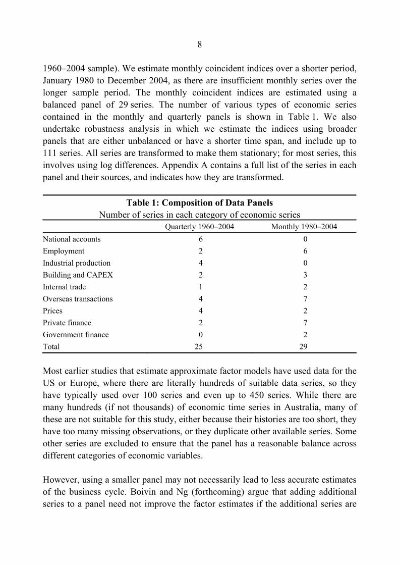
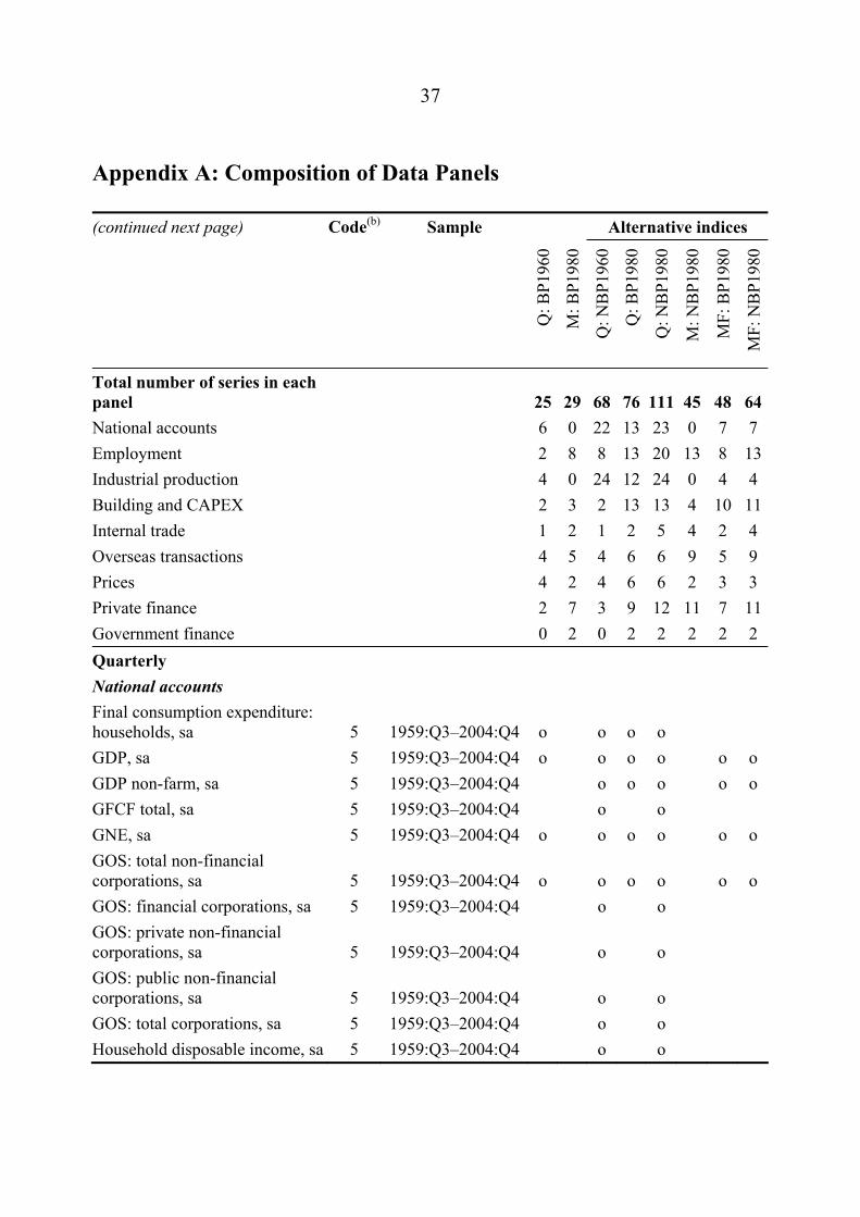
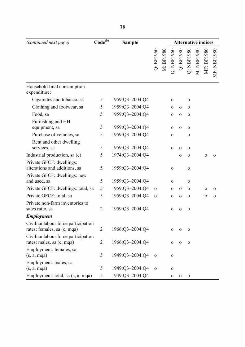
1960–2004 sample). We estimate monthly coincident indices over a shorter period, January 1980 to December 2004, as there are insufficient monthly series over the longer sample period. The monthly coincident indices are estimated using a balanced panel of 29 series. The number of various types of economic series contained in the monthly and quarterly panels is shown in Table 1. We also undertake robustness analysis in which we estimate the indices using broader panels that are either unbalanced or have a shorter time span, and include up to 111 series. All series are transformed to make them stationary; for most series, this involves using log differences. Appendix A contains a full list of the series in each panel and their sources, and indicates how they are transformed.

Table 1: Composition of Data Panels Number of series in each category of economic series

Quarterly 1960–2004 Monthly 1980–2004 National accounts 6 0 Employment 2 6 Industrial production 4 0 Building and CAPEX 2 3 Internal trade 1 2 Overseas transactions 4 7 Prices 4 2 Private finance 2 7 Government finance 0 2 Total 25 29 Most earlier studies that estimate approximate factor models have used data for the US or Europe, where there are literally hundreds of suitable data series, so they have typically used over 100 series and even up to 450 series. While there are many hundreds (if not thousands) of economic time series in Australia, many of these are not suitable for this study, either because their histories are too short, they have too many missing observations, or they duplicate other available series. Some other series are excluded to ensure that the panel has a reasonable balance across different categories of economic variables.

However, using a smaller panel may not necessarily lead to less accurate estimates of the business cycle. Boivin and Ng (forthcoming) argue that adding additional series to a panel need not improve the factor estimates if the additional series are

9

noisy or have correlated errors. In previous applications, larger panels have typically been obtained by disaggregating series into their sectoral or regional components (for example, employment in different industries, or housing approvals in particular areas). Such series are likely to contain more idiosyncratic noise, and are likely to have correlated idiosyncratic components. Indeed, Boivin and Ng find that the factors from a panel with as few as 40 series sometimes produce more accurate forecasts than those derived from a panel of 147 series. Watson (2001) also finds that the marginal improvement in forecasting performance from using greater than 50 series is very small. And Inklaar et al (2003) find that they can produce an index that closely matches the EuroCOIN index using a subset of just 38 of the 246 series that are used in constructing the EuroCOIN index.

5. Results

In Section 5.1 we present the coincident indices constructed with quarterly data for the period 1960–2004, and analyse their robustness to alternative specifications. In Section 5.2 we present the indices constructed with monthly data for the period 1980–2004, and consider their robustness.4

5.1 Quarterly Coincident Indices

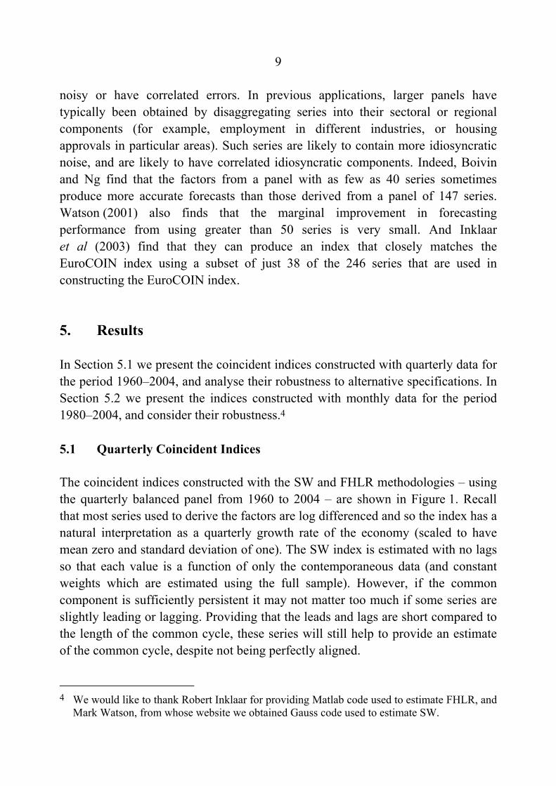
The coincident indices constructed with the SW and FHLR methodologies – using the quarterly balanced panel from 1960 to 2004 – are shown in Figure 1. Recall that most series used to derive the factors are log differenced and so the index has a natural interpretation as a quarterly growth rate of the economy (scaled to have mean zero and standard deviation of one). The SW index is estimated with no lags so that each value is a function of only the contemporaneous data (and constant weights which are estimated using the full sample). However, if the common component is sufficiently persistent it may not matter too much if some series are slightly leading or lagging. Providing that the leads and lags are short compared to the length of the common cycle, these series will still help to provide an estimate of the common cycle, despite not being perfectly aligned.

4 We would like to thank Robert Inklaar for providing Matlab code used to estimate FHLR, and Mark Watson, from whose website we obtained Gauss code used to estimate SW.

10

Figure 1: Quarterly Coincident Indices

-2

0

2

4

-2

0

2

4

-4-3-2-1012

-4-3-2-1012

SW

%GDP(a)

Coincident indices

FHLR

%

% %

20041998199219861980197419681962 Note: (a) 100 × log difference of GDP

Sources: ABS; authors’ calculations

As discussed in Section 3, an information criterion can be used with the SW methodology to determine the number of factors required to explain the panel. The information criterion finds that there is only one factor, and so our SW index is simply the first factor, that is the first principal component. This first factor explains 23 per cent of the variation in the panel of 25 series. For the FHLR index, the explanatory power threshold selects two factors. These two factors explain 37 per cent of the total variance in the panel.

As can be seen in Figure 1, the two indices are very similar; indeed their correlation is 0.91. The most apparent difference is that the FHLR index is somewhat smoother because it removes high-frequency volatility by construction (as is discussed further below). Note also that the FHLR index is shorter by three quarters at both its beginning and end, because it requires leads and lags to estimate the spectral density matrix.

Both series are substantially smoother than quarterly changes in GDP (throughout we use 100 × log difference of GDP, to be consistent with the log differences used in the construction of the indices). It is not surprising that the FHLR index is less volatile than GDP as it is constructed as a two-sided filter, that is, using data either

11

side of a given quarter to provide a smoother indicator, and is additionally smoothed by removing high-frequency movements. But the value of the SW index in a given quarter is constructed from only data in that quarter – it is not smoothed in any way other than the fact that it uses the cross-section of data. Further, the SW index uses only the first factor, while the FHLR index is an average of two factors.

There are clear economic cycles in the two constructed coincident indices, while it takes a more highly trained eye to discern a cycle in the quarterly changes in GDP. Both of our indices show three major downturns in economic activity over the 45-year period; in the mid 1970s, the early 1980s and the early 1990s. Smaller economic downturns show up clearly in the early and late 1970s, the mid 1980s, and a spike down in 2000 associated with the introduction of the GST. The long boom of the 1960s is evident with both indices around one standard deviation above zero for much of the decade. The past ten years or so have also seen the indices being positive on average, indicating stronger-than-average economic conditions.

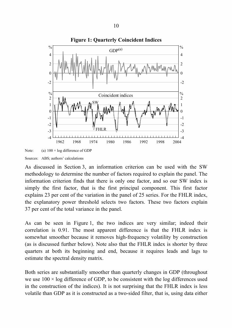
Annual growth rates are often used to get a smoother picture of GDP growth. However, Figure 2 shows that annual GDP growth is still much noisier than the annual change in the SW index (the four-quarter sum, scaled to have the same mean and variance as annual GDP growth). The FHLR index is not shown since the annual changes are almost identical to those of the SW index.

While the scaled growth in the SW index is typically around the same rate as GDP, differences do open up at times. Indeed, the SW index has been notably stronger than GDP growth over the past few years. This presumably reflects the relative importance of some series that have been very strong over this period (including employment and domestic demand).

12

Figure 2: Annual Rates of Change

-4

-2

0

2

4

6

8

-4

-2

0

2

4

6

8GDP

%

SW(a)

1992

%

200419741962 198619801968 1998 Note: (a) SW is the 4-quarter rolling sum of the SW quarterly index, scaled to have the same mean and variance

as annual GDP growth. For consistency, GDP growth is also measured as the 4-quarter log difference.

Sources: ABS; authors’ calculations

5.1.1 Robustness of the quarterly indices

As discussed in Sections 2 and 3, the number of factors that are combined to form an index, and the composition of the panel used for estimation, will influence the behaviour of that coincident index. We examine the sensitivity of the SW and FHLR indices along these two dimensions.5 Firstly, we construct both indices using alternative numbers of factors. Secondly, both indices are estimated using a much broader panel of 76 series that are available from 1980. We also examine the sensitivity to the breadth and composition of the panel by using even broader panels that are not balanced (that is they contain some missing observations) which can be used with the SW methodology. The non-balanced panels starting in 1960 and 1980 contain 68 and 111 series, respectively.

5 We also examined the robustness of the indices to correction for outliers. Setting extreme values (say, those greater than four or ten times the interquartile range) to either missing values or maximum values generally has little effect on the estimated indices. The indices are also robust to using a panel of data in which large consecutive offsetting observations (for example a normalised growth rate of –5 per cent followed by +5 per cent), which possibly represent timing issues in the data, are smoothed.

13

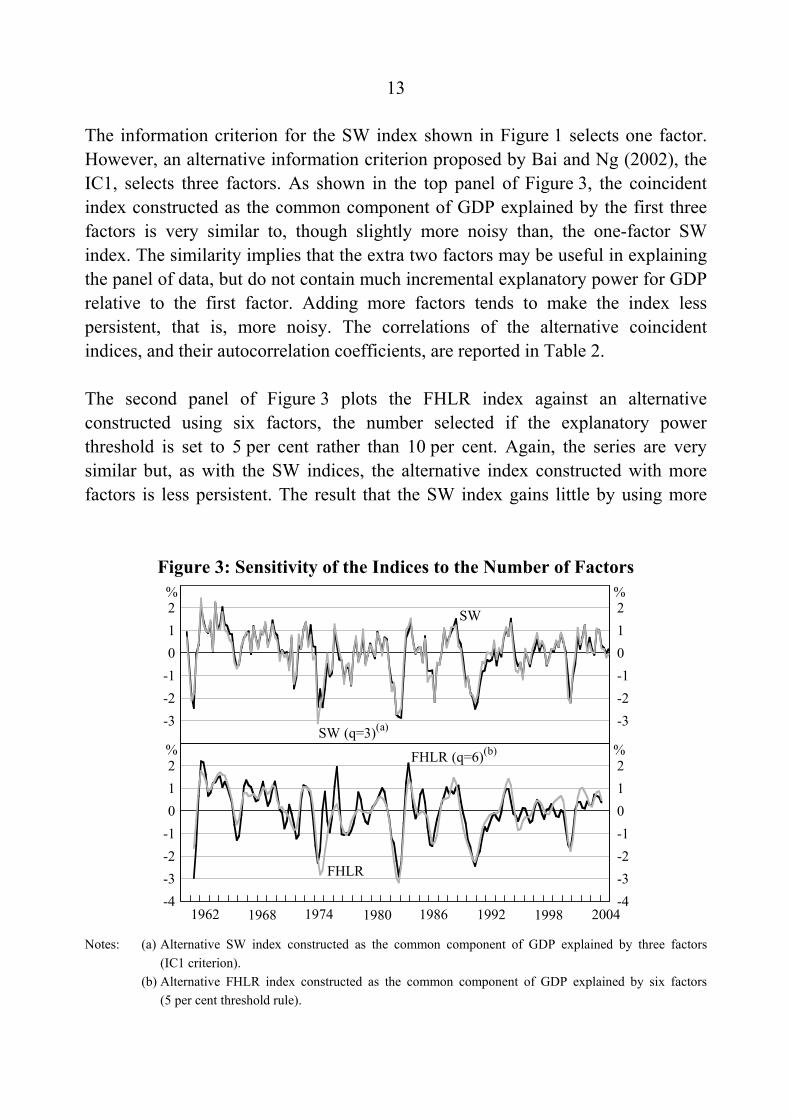
The information criterion for the SW index shown in Figure 1 selects one factor. However, an alternative information criterion proposed by Bai and Ng (2002), the IC1, selects three factors. As shown in the top panel of Figure 3, the coincident index constructed as the common component of GDP explained by the first three factors is very similar to, though slightly more noisy than, the one-factor SW index. The similarity implies that the extra two factors may be useful in explaining the panel of data, but do not contain much incremental explanatory power for GDP relative to the first factor. Adding more factors tends to make the index less persistent, that is, more noisy. The correlations of the alternative coincident indices, and their autocorrelation coefficients, are reported in Table 2.

The second panel of Figure 3 plots the FHLR index against an alternative constructed using six factors, the number selected if the explanatory power threshold is set to 5 per cent rather than 10 per cent. Again, the series are very similar but, as with the SW indices, the alternative index constructed with more factors is less persistent. The result that the SW index gains little by using more

Figure 3: Sensitivity of the Indices to the Number of Factors

-3-2-1012

-3-2-1012

-4-3-2-1012

-4-3-2-1012

SW

%

1962

%%

%

1968 1974 1980 1986 1992 1998 2004

SW (q=3)(a)

FHLR (q=6)(b)

FHLR

Notes: (a) Alternative SW index constructed as the common component of GDP explained by three factors

(IC1 criterion). (b) Alternative FHLR index constructed as the common component of GDP explained by six factors

(5 per cent threshold rule).

14

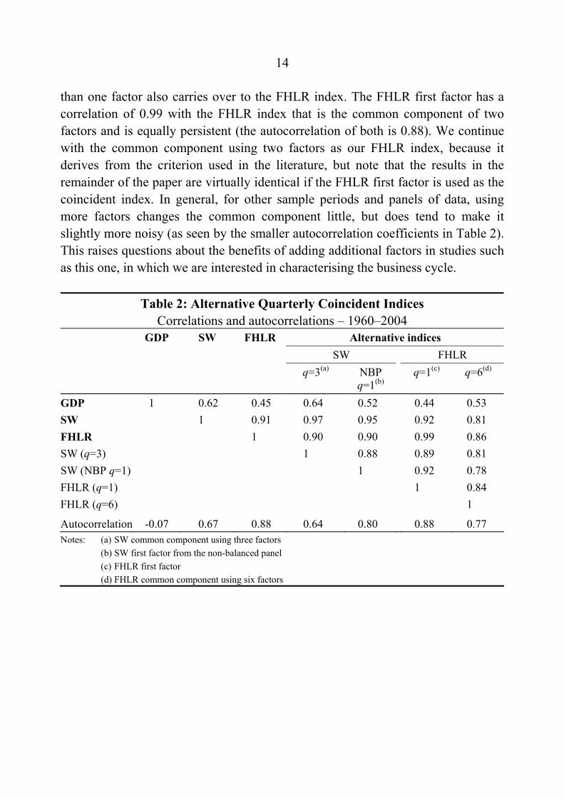
than one factor also carries over to the FHLR index. The FHLR first factor has a correlation of 0.99 with the FHLR index that is the common component of two factors and is equally persistent (the autocorrelation of both is 0.88). We continue with the common component using two factors as our FHLR index, because it derives from the criterion used in the literature, but note that the results in the remainder of the paper are virtually identical if the FHLR first factor is used as the coincident index. In general, for other sample periods and panels of data, using more factors changes the common component little, but does tend to make it slightly more noisy (as seen by the smaller autocorrelation coefficients in Table 2). This raises questions about the benefits of adding additional factors in studies such as this one, in which we are interested in characterising the business cycle.

Table 2: Alternative Quarterly Coincident Indices Correlations and autocorrelations – 1960–2004

GDP SW FHLR Alternative indices SW FHLR q=3(a) NBP

q=1(b) q=1(c) q=6(d)

GDP 1 0.62 0.45 0.64 0.52 0.44 0.53 SW 1 0.91 0.97 0.95 0.92 0.81 FHLR 1 0.90 0.90 0.99 0.86 SW (q=3) 1 0.88 0.89 0.81 SW (NBP q=1) 1 0.92 0.78 FHLR (q=1) 1 0.84 FHLR (q=6) 1

Autocorrelation -0.07 0.67 0.88 0.64 0.80 0.88 0.77 Notes: (a) SW common component using three factors (b) SW first factor from the non-balanced panel (c) FHLR first factor (d) FHLR common component using six factors

15

Using a broader, non-balanced, panel with 68 series for the period 1960–2004 also makes little difference to the estimated SW coincident index. The alternative SW index estimated with this broader panel has a correlation of 0.95 with the SW index (column 5 of Table 2).6

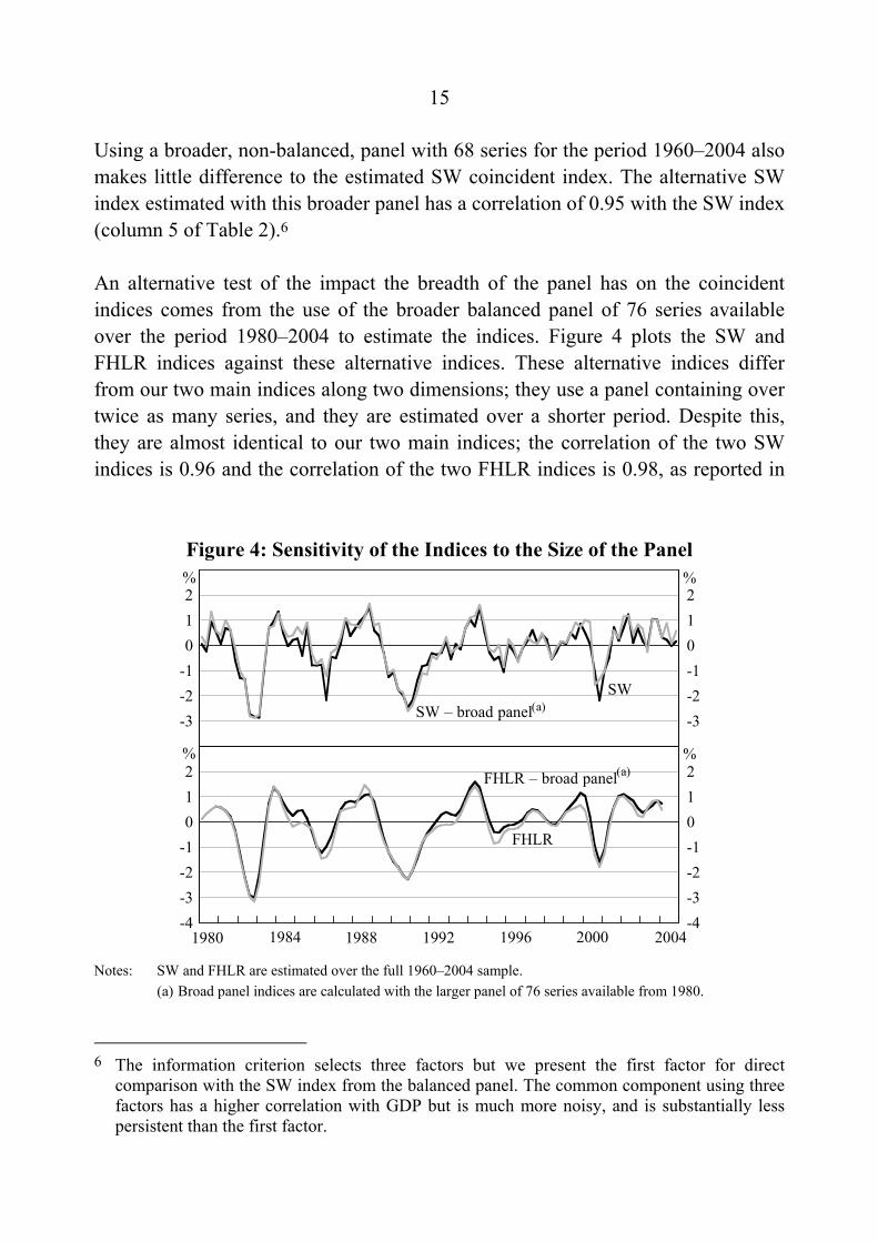
An alternative test of the impact the breadth of the panel has on the coincident indices comes from the use of the broader balanced panel of 76 series available over the period 1980–2004 to estimate the indices. Figure 4 plots the SW and FHLR indices against these alternative indices. These alternative indices differ from our two main indices along two dimensions; they use a panel containing over twice as many series, and they are estimated over a shorter period. Despite this, they are almost identical to our two main indices; the correlation of the two SW indices is 0.96 and the correlation of the two FHLR indices is 0.98, as reported in

Figure 4: Sensitivity of the Indices to the Size of the Panel

-3-2-1012

-3-2-1012

-4-3-2-1012

-4-3-2-1012

FHLR

%

SW

FHLR – broad panel(a)

SW – broad panel(a)

2004

% %

%

199219881980 1984 1996 2000 Notes: SW and FHLR are estimated over the full 1960–2004 sample. (a) Broad panel indices are calculated with the larger panel of 76 series available from 1980.

6 The information criterion selects three factors but we present the first factor for direct comparison with the SW index from the balanced panel. The common component using three factors has a higher correlation with GDP but is much more noisy, and is substantially less persistent than the first factor.

16

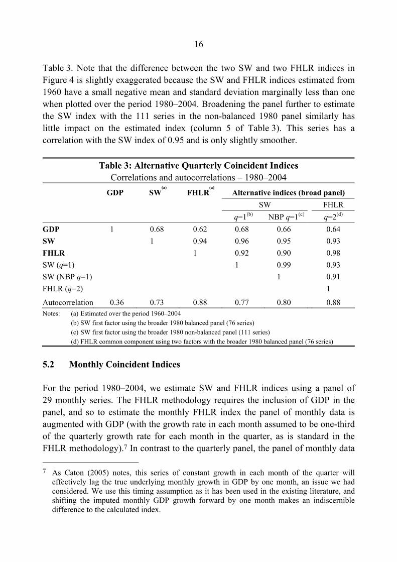
Table 3. Note that the difference between the two SW and two FHLR indices in Figure 4 is slightly exaggerated because the SW and FHLR indices estimated from 1960 have a small negative mean and standard deviation marginally less than one when plotted over the period 1980–2004. Broadening the panel further to estimate the SW index with the 111 series in the non-balanced 1980 panel similarly has little impact on the estimated index (column 5 of Table 3). This series has a correlation with the SW index of 0.95 and is only slightly smoother.

Table 3: Alternative Quarterly Coincident Indices Correlations and autocorrelations – 1980–2004

GDP SW(a)

FHLR(a)

Alternative indices (broad panel) SW FHLR q=1(b) NBP q=1(c) q=2(d) GDP 1 0.68 0.62 0.68 0.66 0.64 SW 1 0.94 0.96 0.95 0.93 FHLR 1 0.92 0.90 0.98 SW (q=1) 1 0.99 0.93 SW (NBP q=1) 1 0.91 FHLR (q=2) 1

Autocorrelation 0.36 0.73 0.88 0.77 0.80 0.88 Notes: (a) Estimated over the period 1960–2004 (b) SW first factor using the broader 1980 balanced panel (76 series) (c) SW first factor using the broader 1980 non-balanced panel (111 series) (d) FHLR common component using two factors with the broader 1980 balanced panel (76 series)

5.2 Monthly Coincident Indices

For the period 1980–2004, we estimate SW and FHLR indices using a panel of 29 monthly series. The FHLR methodology requires the inclusion of GDP in the panel, and so to estimate the monthly FHLR index the panel of monthly data is augmented with GDP (with the growth rate in each month assumed to be one-third of the quarterly growth rate for each month in the quarter, as is standard in the FHLR methodology).7 In contrast to the quarterly panel, the panel of monthly data

7 As Caton (2005) notes, this series of constant growth in each month of the quarter will effectively lag the true underlying monthly growth in GDP by one month, an issue we had considered. We use this timing assumption as it has been used in the existing literature, and shifting the imputed monthly GDP growth forward by one month makes an indiscernible difference to the calculated index.

17

has no national accounts series (household income, etc) and no measures of production. Rather it contains proportionately more overseas sector variables (trade, the exchange rate, etc) and private finance variables (credit, lending approvals, etc). Every effort is made to keep this panel as representative as possible, but given that some types of series are not produced at a monthly frequency they are obviously under-represented. The sensitivity to this constraint is considered in Section 5.2.1 with the construction of mixed-frequency indices that also include some of these quarterly series.

The quarterly SW index is estimated with no lags, as the series in the panel are taken to be mostly contemporaneously related at a quarterly frequency. This assumption is validated by the fact that FHLR places relatively small (and generally reasonably symmetrical) weights on leads and lags, and the close contemporaneous relationship of the FHLR index with the SW index. However, leads and lags are presumably more important in constructing a monthly index. To account for this we estimate the SW index using a stacked panel (with s=2 in Equation (1)). We interpret this model as having one lead and one lag, rather than two lags. This alignment of the index corresponds better with the path of the economic series and the FHLR index.

In a dynamic factor model, in which the data depend on leads and lags of the factors, the Bai and Ng (2002) information criteria will only provide an upper bound for the number of factors relevant for the model.8 The IC2 information criterion selects two factors. However, the weight on the second factor in the regression of GDP on the two factors is very small and so we present the first factor as our monthly SW index (the correlation of the two-factor common component with the first factor is 0.99).9 As for the quarterly index, the 5 per cent threshold criterion selects two factors for the monthly FHLR index. The SW and

8 In the SW setting this can be seen because the estimation technique does not recognise that ft

and ft–1 are the same factors. Therefore, the information criteria will provide a guide to r rather than q.

9 To determine the weights to combine the factors we regress GDP on the monthly factors. GDP is assumed to grow at one-third of the quarterly rate in each month of the quarter. This assumption is consistent with the assumption made about GDP growth in construction of the monthly FHLR index.

18

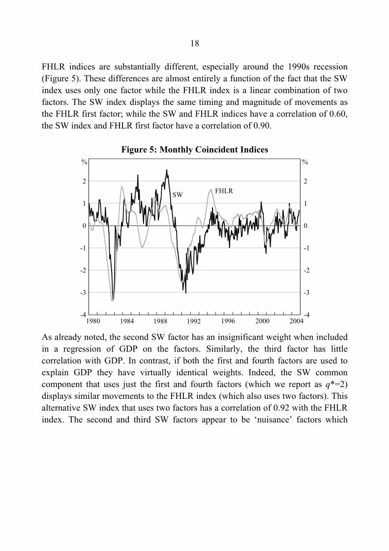
FHLR indices are substantially different, especially around the 1990s recession (Figure 5). These differences are almost entirely a function of the fact that the SW index uses only one factor while the FHLR index is a linear combination of two factors. The SW index displays the same timing and magnitude of movements as the FHLR first factor; while the SW and FHLR indices have a correlation of 0.60, the SW index and FHLR first factor have a correlation of 0.90.

Figure 5: Monthly Coincident Indices

-4

-3

-2

-1

0

1

2

-4

-3

-2

-1

0

1

2

SW

%

FHLR

1984

%

1988 1992 20041980 20001996 As already noted, the second SW factor has an insignificant weight when included in a regression of GDP on the factors. Similarly, the third factor has little correlation with GDP. In contrast, if both the first and fourth factors are used to explain GDP they have virtually identical weights. Indeed, the SW common component that uses just the first and fourth factors (which we report as q*=2) displays similar movements to the FHLR index (which also uses two factors). This alternative SW index that uses two factors has a correlation of 0.92 with the FHLR index. The second and third SW factors appear to be ‘nuisance’ factors which

19

result from the use of a stacked panel.10 While the business cycle could be well characterised by one factor for the quarterly panel of data, in the monthly case there are two factors that each represent different cycles, and so a common component of the two may better characterise the business cycle. The main difference between the SW and FHLR indices that use the same number of factors is that FHLR indices are smoother, largely because, by construction, they remove high-frequency volatility. This comes at the expense of the estimation procedure truncating the beginning and end of the sample. The FHLR index also incorporates information from four leads and four lags while the SW index has just one lead and one lag.

5.2.1 Robustness of the monthly indices

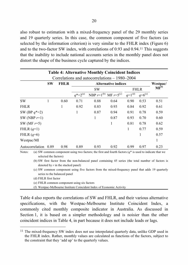
As discussed in the previous section, the monthly coincident indices are sensitive to whether one or two factors are used in their construction, unlike the quarterly indices for which the cycle changes little with the use of more factors (though the amount of noise in the index does change). However, the indices do seem to be fairly robust to the use of more than two factors in their construction. For example, Table 4 shows that the monthly FHLR index, which uses two factors, has a correlation of 0.92 with the alternative FHLR index that combines six factors (the number determined by the 5 per cent threshold) and the persistence is essentially unchanged.

At the monthly frequency, the correlations of the coincident indices using alternative specifications are lower than at the quarterly frequency. However, the monthly SW index is quite robust to using a broader panel; for example, the SW index has a correlation coefficient of 0.88 with an alternative index using the non-balanced panel with 45 series that also only uses the first factor. The SW index is

10 The second and third factors have small weights when included in a regression of GDP on the first four factors. They are very noisy, with autocorrelation coefficients of –0.63 and –0.55. This is seemingly the result of using a stacked panel. We also find negatively autocorrelated factors, though weaker than for Australia, when stacking the panel used to construct the CFNAI. We thank Mark Watson and Jim Stock for discussing this point with us, and Watson for the following intuitive example. Suppose the data panel is explained by only one factor, which is positively autocorrelated, ttt ff ηρ += −1 . Then the stacked panel, which augments the data matrix with one lag, will be spanned by two factors. Since they must be orthogonal, if one factor is ft + ft–1 the other could be ft – ft–1. In this example, the second factor from the stacked panel will be negatively autocorrelated even though the true factor is not.

20

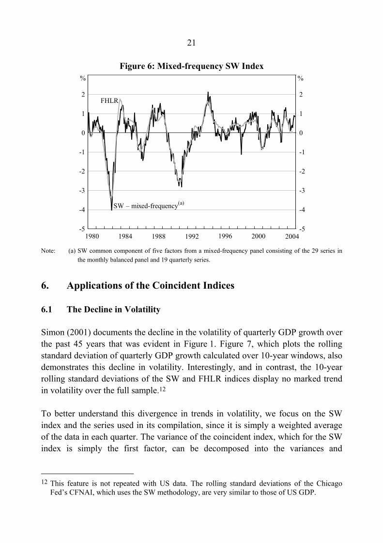
also robust to estimation with a mixed-frequency panel of the 29 monthly series and 19 quarterly series. In this case, the common component of five factors (as selected by the information criterion) is very similar to the FHLR index (Figure 6) and to the two-factor SW index, with correlations of 0.93 and 0.94.11 This suggests that the inability to include national accounts series in the monthly panel does not distort the shape of the business cycle captured by the indices.

Table 4: Alternative Monthly Coincident Indices Correlations and autocorrelations – 1980–2004

SW FHLR Alternative indices SW FHLR q*=2(a) NBP r=1(b) MF r=5(c) q=1(d) q=6(e)

Westpac/MI(f)

SW 1 0.60 0.71 0.88 0.64 0.90 0.53 0.51 FHLR 1 0.92 0.83 0.93 0.84 0.92 0.61 SW (BP q*=2) 1 0.87 0.94 0.91 0.78 0.59 SW (NBP r=1) 1 0.87 0.93 0.70 0.60 SW (MF r=5) 1 0.81 0.78 0.62 FHLR (q=1) 1 0.77 0.59 FHLR (q=6) 1 0.57 Westpac/MI 1

Autocorrelation 0.89 0.98 0.89 0.93 0.92 0.99 0.97 0.23 Notes: (a) SW common component using two factors; the first and fourth factors (q* is used to indicate that we

selected the factors) (b) SW first factor from the non-balanced panel containing 45 series (the total number of factors is

denoted by r in the stacked panel) (c) SW common component using five factors from the mixed-frequency panel that adds 19 quarterly

series to the balanced panel (d) FHLR first factor (e) FHLR common component using six factors (f) Westpac-Melbourne Institute Coincident Index of Economic Activity

Table 4 also reports the correlations of SW and FHLR, and their various alternative specifications, with the Westpac-Melbourne Institute Coincident Index, a commonly cited monthly composite indicator in Australia. As discussed in Section 1, it is based on a simpler methodology and is noisier than the other coincident indices in Table 4, in part because it does not include leads or lags.

11 The mixed-frequency SW index does not use interpolated quarterly data, unlike GDP used in the FHLR index. Rather, monthly values are calculated as functions of the factors, subject to the constraint that they ‘add up’ to the quarterly values.

21

Figure 6: Mixed-frequency SW Index

-5

-4

-3

-2

-1

0

1

2

-5

-4

-3

-2

-1

0

1

2

SW – mixed-frequency(a)

%

FHLR

1980

%

1984 1988 1992 1996 2000 2004 Note: (a) SW common component of five factors from a mixed-frequency panel consisting of the 29 series in

the monthly balanced panel and 19 quarterly series.

6. Applications of the Coincident Indices

6.1 The Decline in Volatility

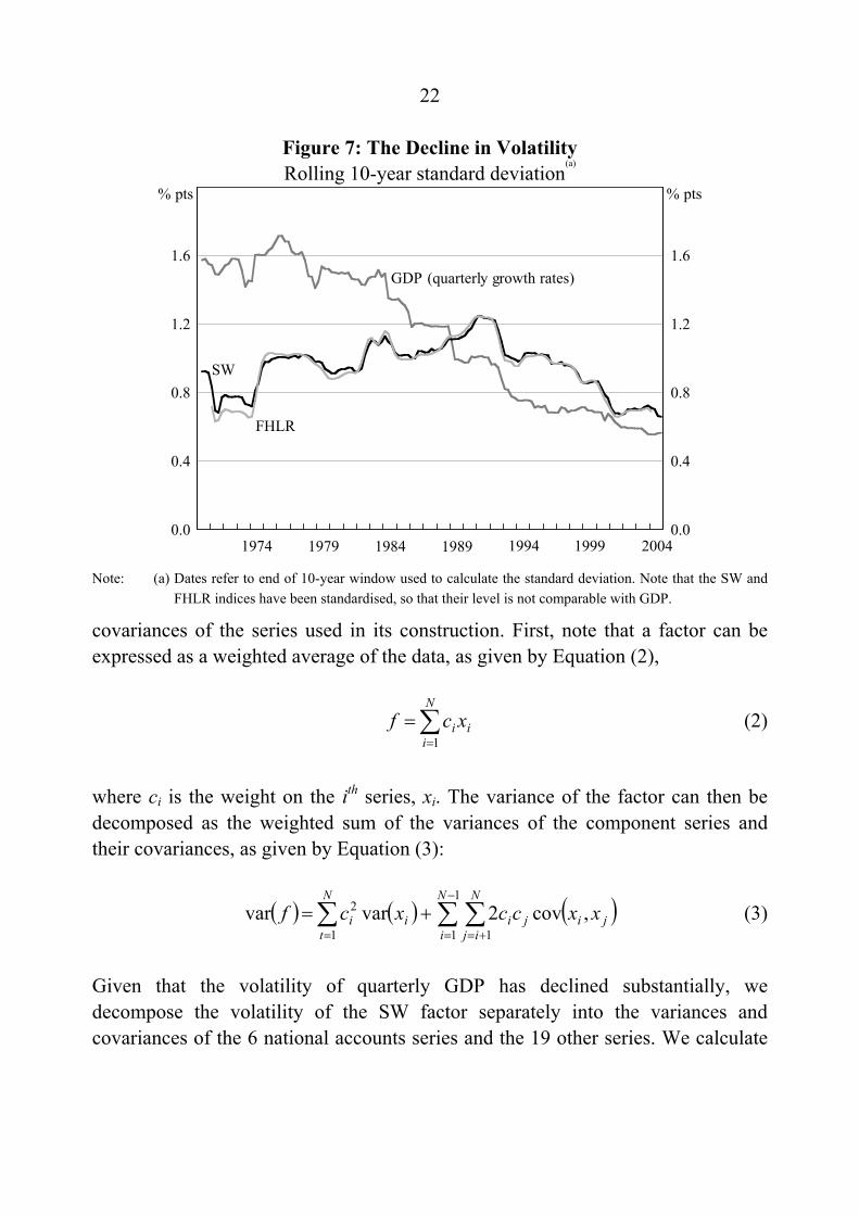
Simon (2001) documents the decline in the volatility of quarterly GDP growth over the past 45 years that was evident in Figure 1. Figure 7, which plots the rolling standard deviation of quarterly GDP growth calculated over 10-year windows, also demonstrates this decline in volatility. Interestingly, and in contrast, the 10-year rolling standard deviations of the SW and FHLR indices display no marked trend in volatility over the full sample.12

To better understand this divergence in trends in volatility, we focus on the SW index and the series used in its compilation, since it is simply a weighted average of the data in each quarter. The variance of the coincident index, which for the SW index is simply the first factor, can be decomposed into the variances and

12 This feature is not repeated with US data. The rolling standard deviations of the Chicago Fed’s CFNAI, which uses the SW methodology, are very similar to those of US GDP.

22

Figure 7: The Decline in Volatility Rolling 10-year standard deviation

(a)

0.0

0.4

0.8

1.2

1.6

0.0

0.4

0.8

1.2

1.6GDP (quarterly growth rates)

2004

SW

FHLR

1974 1979 1984 1989 1994 1999

% pts% pts

Note: (a) Dates refer to end of 10-year window used to calculate the standard deviation. Note that the SW and

FHLR indices have been standardised, so that their level is not comparable with GDP.

covariances of the series used in its construction. First, note that a factor can be expressed as a weighted average of the data, as given by Equation (2),

(2) ∑=

=N

iii xcf

1

where ci is the weight on the ith series, xi. The variance of the factor can then be decomposed as the weighted sum of the variances of the component series and their covariances, as given by Equation (3):

( ) ( ) (∑ ∑ ∑=

)−

= +=+=

N

t

N

i

N

ijjijiii xxccxcf

1

1

1 1

2 ,cov2varvar (3)

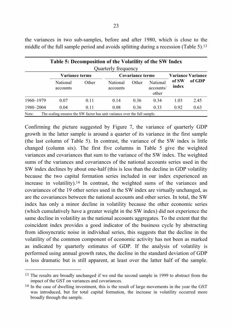
Given that the volatility of quarterly GDP has declined substantially, we decompose the volatility of the SW factor separately into the variances and covariances of the 6 national accounts series and the 19 other series. We calculate

23

the variances in two sub-samples, before and after 1980, which is close to the middle of the full sample period and avoids splitting during a recession (Table 5).13

Table 5: Decomposition of the Volatility of the SW Index Quarterly frequency

Variance terms Covariance terms National

accounts Other National

accounts Other National

accounts/ other

Variance of SW index

Variance of GDP

1960–1979 0.07 0.11 0.14 0.36 0.34 1.03 2.45 1980–2004 0.04 0.11 0.08 0.36 0.33 0.92 0.63 Note: The scaling ensures the SW factor has unit variance over the full sample.

Confirming the picture suggested by Figure 7, the variance of quarterly GDP growth in the latter sample is around a quarter of its variance in the first sample (the last column of Table 5). In contrast, the variance of the SW index is little changed (column six). The first five columns in Table 5 give the weighted variances and covariances that sum to the variance of the SW index. The weighted sums of the variances and covariances of the national accounts series used in the SW index declines by about one-half (this is less than the decline in GDP volatility because the two capital formation series included in our index experienced an increase in volatility).14 In contrast, the weighted sums of the variances and covariances of the 19 other series used in the SW index are virtually unchanged, as are the covariances between the national accounts and other series. In total, the SW index has only a minor decline in volatility because the other economic series (which cumulatively have a greater weight in the SW index) did not experience the same decline in volatility as the national accounts aggregates. To the extent that the coincident index provides a good indicator of the business cycle by abstracting from idiosyncratic noise in individual series, this suggests that the decline in the volatility of the common component of economic activity has not been as marked as indicated by quarterly estimates of GDP. If the analysis of volatility is performed using annual growth rates, the decline in the standard deviation of GDP is less dramatic but is still apparent, at least over the latter half of the sample.

13 The results are broadly unchanged if we end the second sample in 1999 to abstract from the

impact of the GST on variances and covariances.

14 In the case of dwelling investment, this is the result of large movements in the year the GST was introduced, but for total capital formation, the increase in volatility occurred more broadly through the sample.

24

Again, the SW index shows no decline in volatility and the findings from decomposing the volatility of quarterly movements in the SW index carry over to the decomposition using annual changes.

One possible explanation for the divergent trends in volatility is that some of the volatility in GDP in the earlier part of the sample reflects measurement error and that the SW index is able to abstract from such idiosyncratic noise. As GDP has become better measured over time, the volatility of measured GDP has declined.15 Harding (2002) provides further discussion on the decline in the volatility of GDP in Australia, suggesting that it largely reflects reduced measurement errors, and in particular less residual seasonality.16 It may be that other series, such as employment or dwelling approvals, have not had this reduction in measurement error because they have always been easier to measure than GDP. A second explanation is that it may be that the parts of the economy that have experienced a decline in volatility are under-represented in the panel. This would seem less likely as one of the main criteria for selecting the panel of data series is that it should provide a broad representation of the economy. In addition, the magnitude of the decline in sectoral volatilities (or shifts in sectoral shares) that would be required to explain the decline in GDP volatility seems somewhat implausible.

Given the volatility of some economic series has changed it may be that the importance of various series in the construction of the coincident indices has also changed. To examine this, we estimate the SW index over the two sub-samples, 1960–1979 and 1980–2004, using the panel of data that is available over the full

15 There have been a number of improvements in the construction of the national accounts.

These include: the improved methodology for constructing price estimates after the high inflation of the 1970s highlighted problems with the earlier series; the introduction of explicit balance of payments timing adjustments for major commodities from the late 1970s; dating trade flows according to the shipment date rather than the date of recording within the Customs system (backcast to the early 1980s); the development of an import price index (IPI) to replace the RBA’s IPI that was based on export price indices of major trading partners (from the early 1980s); improvements in the profits survey in the early 1980s; and the revamping of the government finance system in the mid 1980s. Many of these initiatives apply to the data from the 1980s onward, suggesting that they may be a factor in the decline in volatility observed around this time. We thank the ABS for bringing to our attention the nature of these changes.

16 However, the ABS examined the issue of residual seasonality and introduced new seasonal factors to address this problem with the release of the June 2002 national accounts.

25

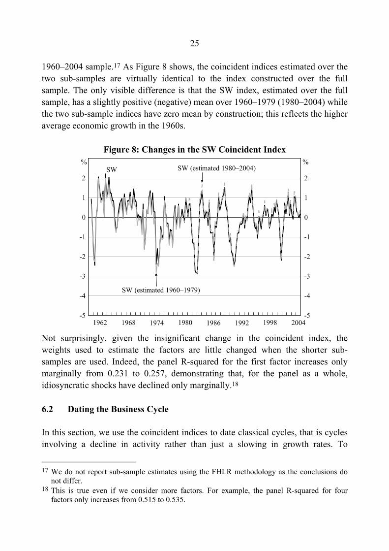
1960–2004 sample.17 As Figure 8 shows, the coincident indices estimated over the two sub-samples are virtually identical to the index constructed over the full sample. The only visible difference is that the SW index, estimated over the full sample, has a slightly positive (negative) mean over 1960–1979 (1980–2004) while the two sub-sample indices have zero mean by construction; this reflects the higher average economic growth in the 1960s.

Figure 8: Changes in the SW Coincident Index

-5

-4

-3

-2

-1

0

1

2

-5

-4

-3

-2

-1

0

1

2SW

1962

%%SW (estimated 1980–2004)

SW (estimated 1960–1979)

1986 1992 1998 20041968 1974 1980 Not surprisingly, given the insignificant change in the coincident index, the weights used to estimate the factors are little changed when the shorter sub-samples are used. Indeed, the panel R-squared for the first factor increases only marginally from 0.231 to 0.257, demonstrating that, for the panel as a whole, idiosyncratic shocks have declined only marginally.18

6.2 Dating the Business Cycle

In this section, we use the coincident indices to date classical cycles, that is cycles involving a decline in activity rather than just a slowing in growth rates. To

17 We do not report sub-sample estimates using the FHLR methodology as the conclusions do

not differ.

18 This is true even if we consider more factors. For example, the panel R-squared for four factors only increases from 0.515 to 0.535.

26

identify periods of recession, we use the Bry and Boschan (1971) algorithm. This is an NBER-style rule that identifies the peaks and troughs in the level of a series and so dates expansions and contractions in an objective manner. Appendix B provides further details on the procedure, including the construction of a levels series from the SW index.

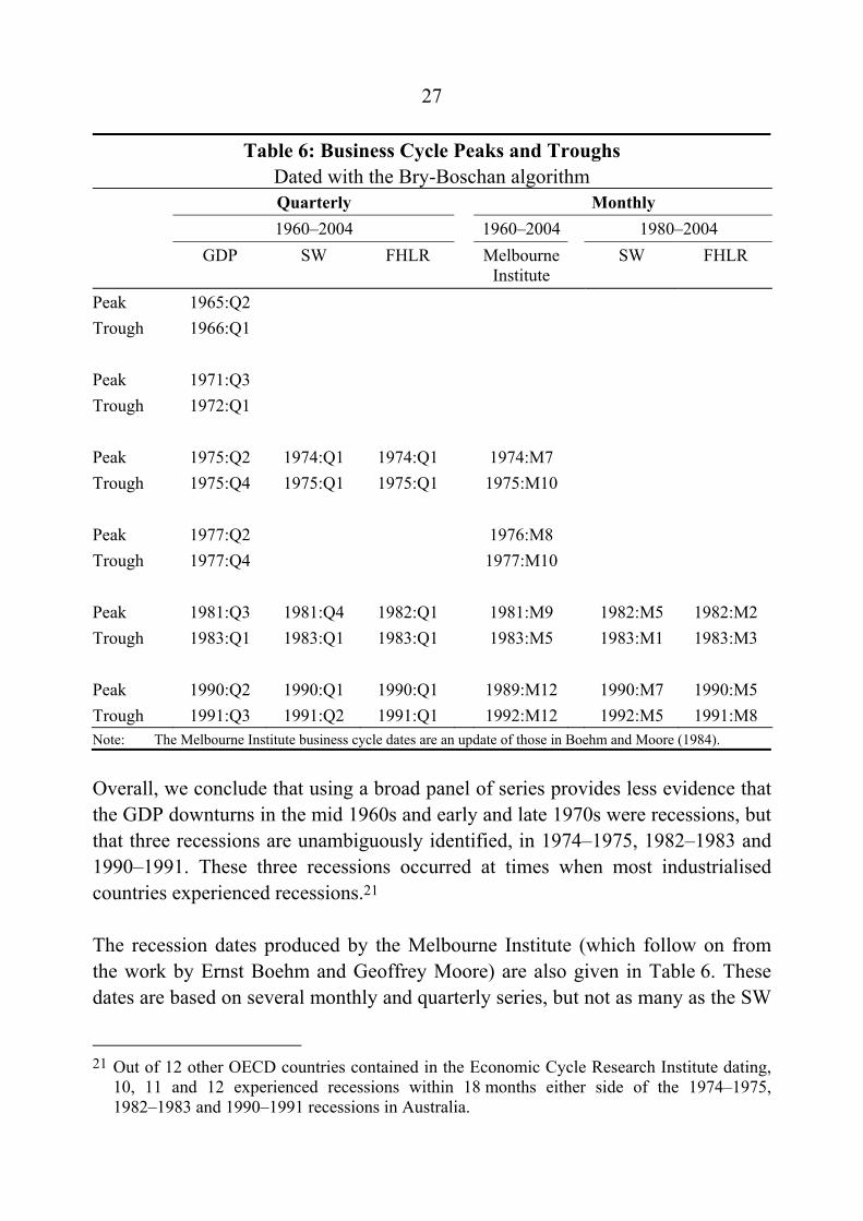
Table 6 reports the recessions identified by GDP and the quarterly SW and FHLR indices.19 While six recessions are located by GDP, only three recessions are identified by the two coincident indices. The three recessions that GDP identifies, but the indices do not, occur in the mid 1960s, and early and late 1970s. As discussed in Section 6.1 the volatility of quarterly GDP growth has declined, while the coincident indices that are based on many series (and statistical weights) have not seen such a reduction in volatility. The greater number of recessions that are identified by GDP appears to be the result of its higher volatility early in the sample. Assuming no change in mean growth rates, higher volatility of measured GDP growth would tend to increase the likelihood of recording (possibly spurious) declines in the level of GDP, and so of recessions being identified in the data.20 Alternatively, we could date the business cycle using non-farm GDP to abstract from the possibility that the volatile farm sector could result in declines in aggregate GDP even when there was no decline in the broader non-farm economy. Unlike GDP, non-farm GDP does not locate recessions in 1965–1966 and 1971–1972, but it does identify the other recessions found in GDP, and an additional recession in the mid 1980s (1985:Q4–1986:Q2). So, abstracting from farm output does reduce the number of recessions identified, but still results in more recessions than the three identified by the coincident indices.

19 As discussed in Appendix B, the dates for the SW index are sensitive to the choice of a

scaling parameter. This does not affect the dates for the FHLR index.

20 For a recession to be identified there will have to be a decline in GDP in at least one quarter. The probability of a fall in GDP will be higher if the volatility of quarterly GDP growth is higher, so making the identification of a recession more likely.

27

Table 6: Business Cycle Peaks and Troughs Dated with the Bry-Boschan algorithm

Quarterly Monthly 1960–2004 1960–2004 1980–2004 GDP SW FHLR Melbourne

Institute SW FHLR

Peak 1965:Q2 Trough 1966:Q1 Peak 1971:Q3 Trough 1972:Q1 Peak 1975:Q2 1974:Q1 1974:Q1 1974:M7 Trough 1975:Q4 1975:Q1 1975:Q1 1975:M10 Peak 1977:Q2 1976:M8 Trough 1977:Q4 1977:M10 Peak 1981:Q3 1981:Q4 1982:Q1 1981:M9 1982:M5 1982:M2 Trough 1983:Q1 1983:Q1 1983:Q1 1983:M5 1983:M1 1983:M3 Peak 1990:Q2 1990:Q1 1990:Q1 1989:M12 1990:M7 1990:M5 Trough 1991:Q3 1991:Q2 1991:Q1 1992:M12 1992:M5 1991:M8 Note: The Melbourne Institute business cycle dates are an update of those in Boehm and Moore (1984).

Overall, we conclude that using a broad panel of series provides less evidence that the GDP downturns in the mid 1960s and early and late 1970s were recessions, but that three recessions are unambiguously identified, in 1974–1975, 1982–1983 and 1990–1991. These three recessions occurred at times when most industrialised countries experienced recessions.21

The recession dates produced by the Melbourne Institute (which follow on from the work by Ernst Boehm and Geoffrey Moore) are also given in Table 6. These dates are based on several monthly and quarterly series, but not as many as the SW

21 Out of 12 other OECD countries contained in the Economic Cycle Research Institute dating, 10, 11 and 12 experienced recessions within 18 months either side of the 1974–1975, 1982–1983 and 1990–1991 recessions in Australia.

28

and FHLR indices. Like these indices, the Melbourne Institute does not date 1965 and 1971 as being recessions. However, they do consider 1976 to have been a recession. This implies that there was an expansion in 1975–1976 that lasted just 10 months.

The monthly SW and FHLR indices (which cover the period 1980–2004) also identify the early 1980s and early 1990s as periods of recession (columns five and six of Table 6). The two indices imply similar timing for the early-1980s recession, but the SW index dates the end of the early-1990s recession nine months later than the FHLR index. This highlights the sensitivity of these monthly indices to the number of factors used to form the index. The SW index which only uses one factor picks up a different cycle to the common component from two factors – the two-factor SW index (q*=2) identifies similar turning points to the FHLR index.

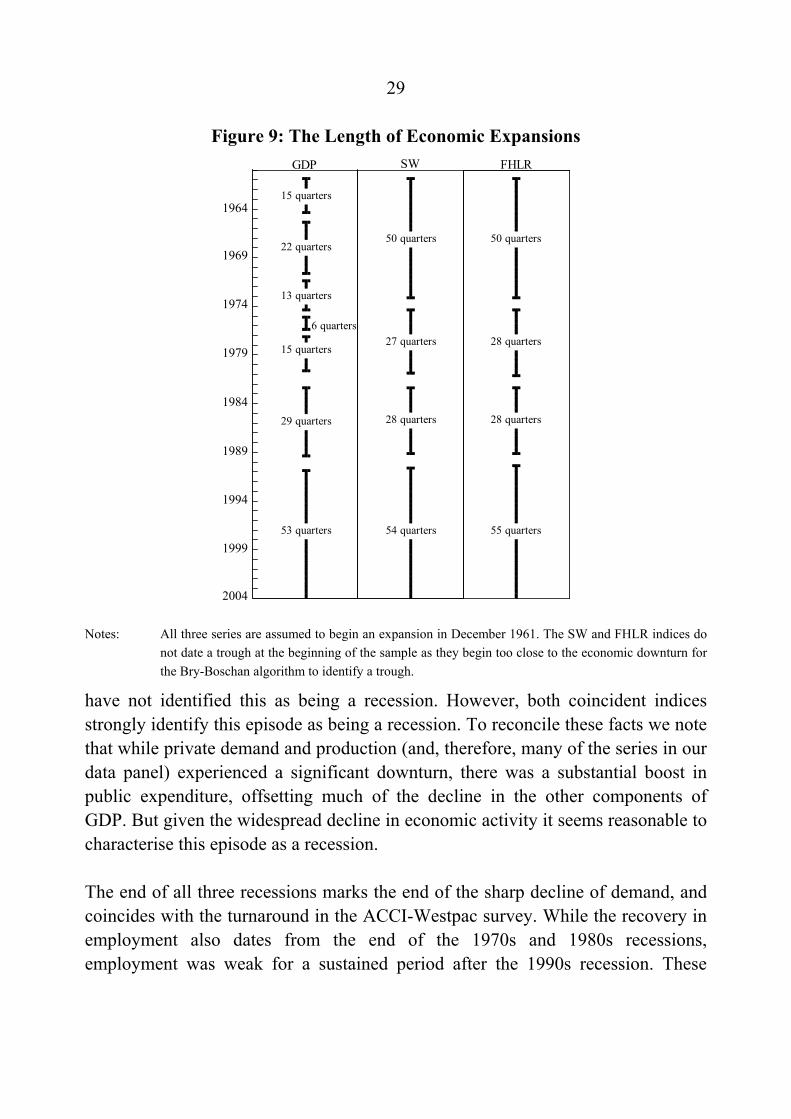
The length of the three main recessions identified in the quarterly data differs only modestly according to whether the dating uses GDP, SW or FHLR. FHLR indicates that all three recessions were four quarters long, while for GDP they range between three and six quarters. In contrast, because GDP and the two indices identify different numbers of recessions, the lengths of the expansions identified differ greatly (Figure 9). Since the use of GDP suggests there have been more recessions, it identifies expansions as being shorter on average, with one lasting only six quarters. This follows from the extra recessions identified by GDP in the 1960s and 1970s, which appear to be the result of the higher level of noise in GDP. The smoother FHLR and SW indices identify a long expansion at the beginning of the sample, two expansions of about seven years each in the middle, and then another ongoing long expansion.

Figure 10 plots GDP along with three representative series – GNE (to capture domestic demand), employment, and the ACCI-Westpac survey of actual output (to capture production) – and highlights the three recessions identified by the SW and FHLR coincident indices. The economic downturn in the three recessions was widespread. In all three recessions, not only did GDP contract, but domestic demand fell, the net balance of actual output from the ACCI-Westpac survey was strongly negative, employment experienced sustained falls, and the unemployment rate increased by over 3 percentage points. The fall in GDP was less severe in the 1974 recession. Indeed, as shown in Appendix C, various vintages of GDP

29

Figure 9: The Length of Economic Expansions

2004

GDP SW FHLR

15 quarters

13 quarters

6 quarters

15 quarters

29 quarters

53 quarters

50 quarters 50 quarters

55 quarters54 quarters

27 quarters

28 quarters 28 quarters

28 quarters

22 quarters

1999

1994

1989

1984

1979

1974

1969

1964

Notes: All three series are assumed to begin an expansion in December 1961. The SW and FHLR indices do

not date a trough at the beginning of the sample as they begin too close to the economic downturn for the Bry-Boschan algorithm to identify a trough.

have not identified this as being a recession. However, both coincident indices strongly identify this episode as being a recession. To reconcile these facts we note that while private demand and production (and, therefore, many of the series in our data panel) experienced a significant downturn, there was a substantial boost in public expenditure, offsetting much of the decline in the other components of GDP. But given the widespread decline in economic activity it seems reasonable to characterise this episode as a recession.

The end of all three recessions marks the end of the sharp decline of demand, and coincides with the turnaround in the ACCI-Westpac survey. While the recovery in employment also dates from the end of the 1970s and 1980s recessions, employment was weak for a sustained period after the 1990s recession. These

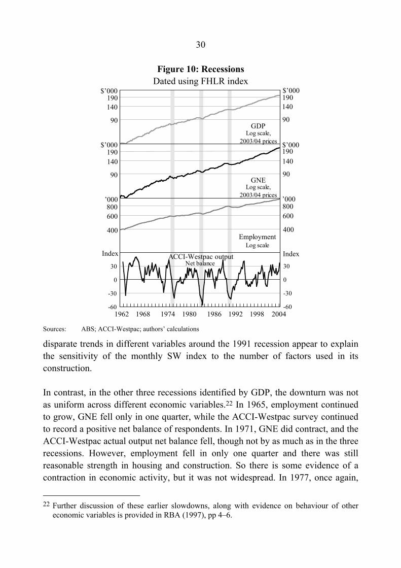
30

Figure 10: Recessions Dated using FHLR index

-60

-30

0

30

-60

-30

0

30

GDP

Net balance

2004

ACCI-Westpac output

1998199219861980197419681962

190140

90

190140

90

190140

90

190140

90

800600

400

800600

400

$’000$’000

$’000$’000

’000’000

Index Index

GNELog scale,

2003/04 prices

EmploymentLog scale

Log scale,2003/04 prices

Sources: ABS; ACCI-Westpac; authors’ calculations

disparate trends in different variables around the 1991 recession appear to explain the sensitivity of the monthly SW index to the number of factors used in its construction.

In contrast, in the other three recessions identified by GDP, the downturn was not as uniform across different economic variables.22 In 1965, employment continued to grow, GNE fell only in one quarter, while the ACCI-Westpac survey continued to record a positive net balance of respondents. In 1971, GNE did contract, and the ACCI-Westpac actual output net balance fell, though not by as much as in the three recessions. However, employment fell in only one quarter and there was still reasonable strength in housing and construction. So there is some evidence of a contraction in economic activity, but it was not widespread. In 1977, once again,

22 Further discussion of these earlier slowdowns, along with evidence on behaviour of other economic variables is provided in RBA (1997), pp 4–6.

31

GNE fell while employment fell in only one of the quarters. But the ACCI-Westpac survey was only slightly negative and investment and exports showed no sign of a downturn.

The constructed indices are less noisy measures of the business cycle than GDP, especially in the early part of the sample, suggesting that there are advantages from using a large range of series and a statistically based set of weights. Notwithstanding the fact that GDP has become less noisy over time, we conjecture that these advantages may also carry over to real-time analysis (though without real-time data for the series used to construct the indices we cannot test this conjecture). Some of the series used in the construction of the indices are not revised, and those series that are revised come from a range of different surveys or collection methods, so that revisions to particular series may be largely independent (and therefore mostly ‘wash out’). In addition, as shown in Section 6.1, the weights in the indices are quite stable between the first and second halves of the sample. In contrast, as Appendix C shows, the identification and timing of recessions can change substantially with revisions to GDP, although it must be noted that the periods of most substantial revisions pre-date methodological improvements in the construction of GDP.

6.3 Changes in International Correlation of Business Cycles

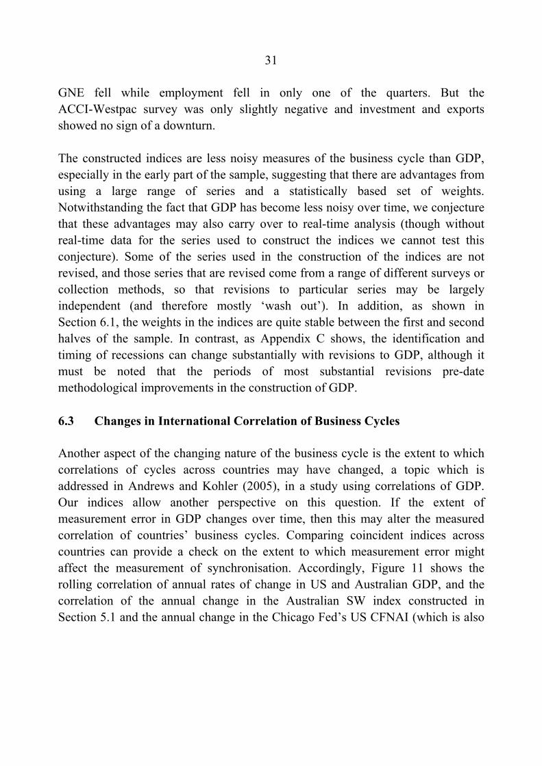
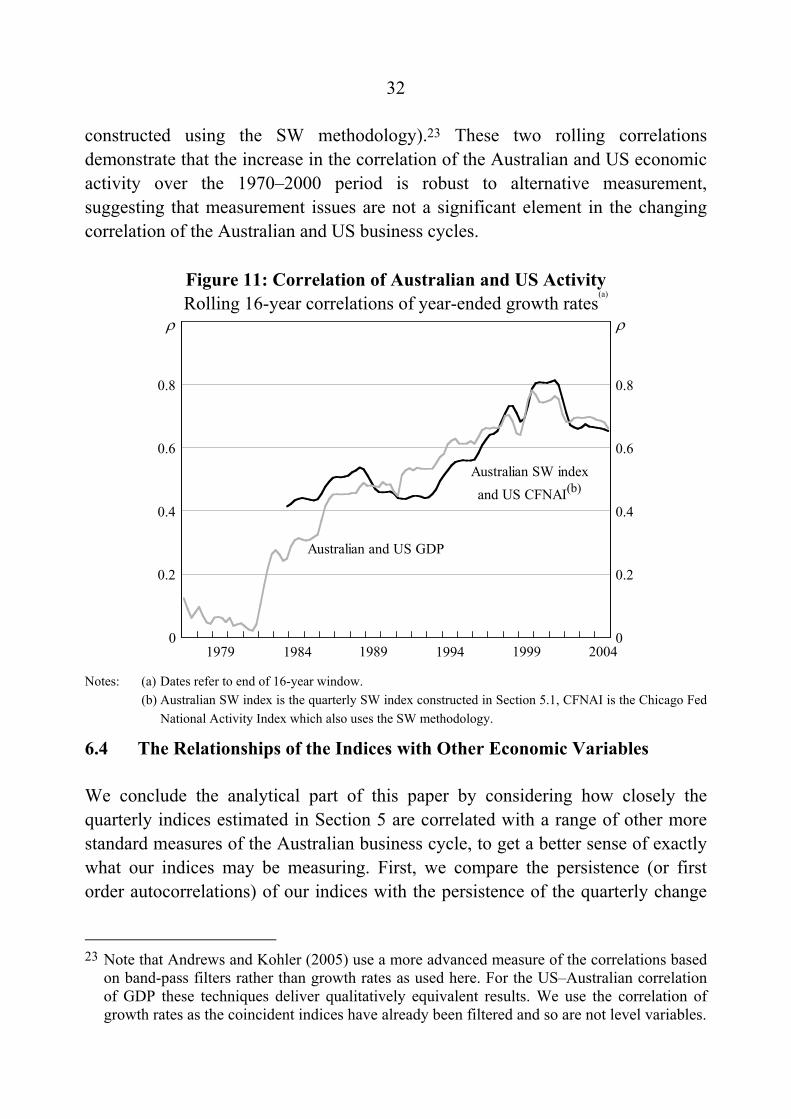
Another aspect of the changing nature of the business cycle is the extent to which correlations of cycles across countries may have changed, a topic which is addressed in Andrews and Kohler (2005), in a study using correlations of GDP. Our indices allow another perspective on this question. If the extent of measurement error in GDP changes over time, then this may alter the measured correlation of countries’ business cycles. Comparing coincident indices across countries can provide a check on the extent to which measurement error might affect the measurement of synchronisation. Accordingly, Figure 11 shows the rolling correlation of annual rates of change in US and Australian GDP, and the correlation of the annual change in the Australian SW index constructed in Section 5.1 and the annual change in the Chicago Fed’s US CFNAI (which is also

32

constructed using the SW methodology).23 These two rolling correlations demonstrate that the increase in the correlation of the Australian and US economic activity over the 1970–2000 period is robust to alternative measurement, suggesting that measurement issues are not a significant element in the changing correlation of the Australian and US business cycles.

Figure 11: Correlation of Australian and US Activity Rolling 16-year correlations of year-ended growth rates

(a)

0

0.2

0.4

0.6

0.8

0

0.2

0.4

0.6

0.8

Australian SW indexand US CFNAI(b)

2004

Australian and US GDP

19991979 199419891984

ρρ

Notes: (a) Dates refer to end of 16-year window. (b) Australian SW index is the quarterly SW index constructed in Section 5.1, CFNAI is the Chicago Fed

National Activity Index which also uses the SW methodology.

6.4 The Relationships of the Indices with Other Economic Variables

We conclude the analytical part of this paper by considering how closely the quarterly indices estimated in Section 5 are correlated with a range of other more standard measures of the Australian business cycle, to get a better sense of exactly what our indices may be measuring. First, we compare the persistence (or first order autocorrelations) of our indices with the persistence of the quarterly change

23 Note that Andrews and Kohler (2005) use a more advanced measure of the correlations based on band-pass filters rather than growth rates as used here. For the US–Australian correlation of GDP these techniques deliver qualitatively equivalent results. We use the correlation of growth rates as the coincident indices have already been filtered and so are not level variables.

33

in GDP and some other standard variables. In principle, the concept of the business cycle is one of a relatively persistent process, so we would expect that a good measure of the cycle should have a relatively high degree of persistence.

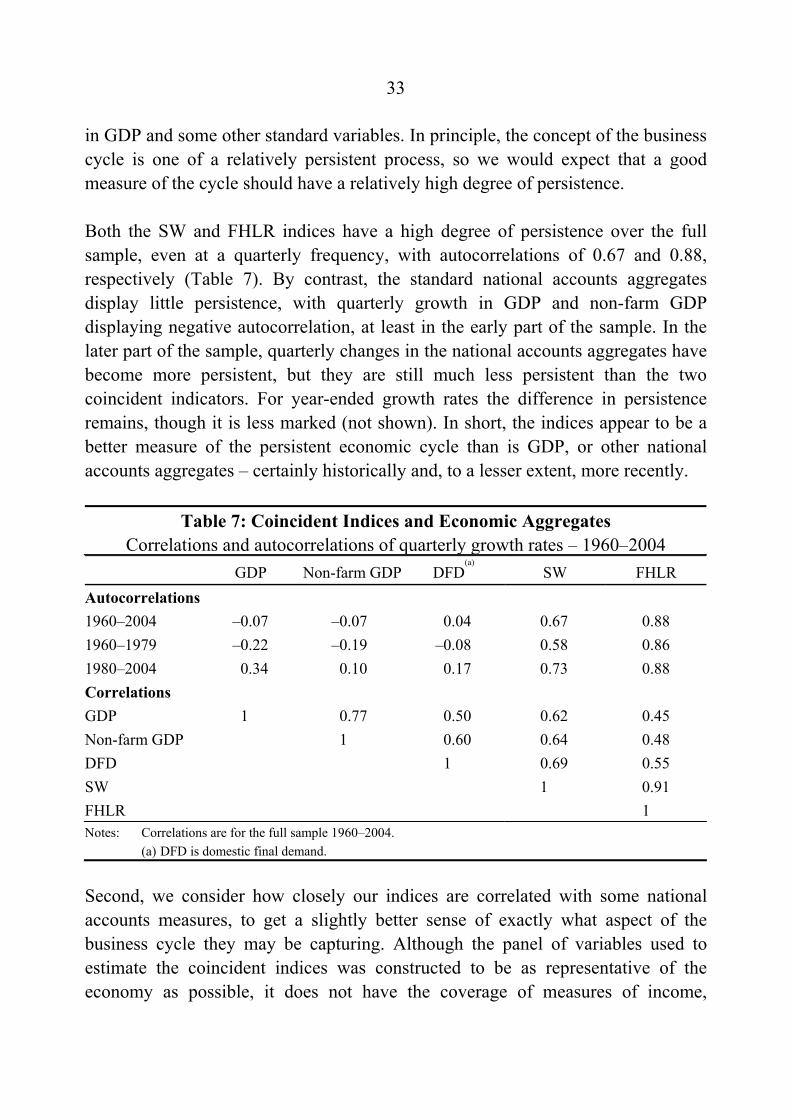
Both the SW and FHLR indices have a high degree of persistence over the full sample, even at a quarterly frequency, with autocorrelations of 0.67 and 0.88, respectively (Table 7). By contrast, the standard national accounts aggregates display little persistence, with quarterly growth in GDP and non-farm GDP displaying negative autocorrelation, at least in the early part of the sample. In the later part of the sample, quarterly changes in the national accounts aggregates have become more persistent, but they are still much less persistent than the two coincident indicators. For year-ended growth rates the difference in persistence remains, though it is less marked (not shown). In short, the indices appear to be a better measure of the persistent economic cycle than is GDP, or other national accounts aggregates – certainly historically and, to a lesser extent, more recently.

Table 7: Coincident Indices and Economic Aggregates Correlations and autocorrelations of quarterly growth rates – 1960–2004

GDP Non-farm GDP DFD(a)

SW FHLR Autocorrelations 1960–2004 –0.07 –0.07 0.04 0.67 0.88 1960–1979 –0.22 –0.19 –0.08 0.58 0.86 1980–2004 0.34 0.10 0.17 0.73 0.88 Correlations GDP 1 0.77 0.50 0.62 0.45 Non-farm GDP 1 0.60 0.64 0.48 DFD 1 0.69 0.55 SW 1 0.91 FHLR 1 Notes: Correlations are for the full sample 1960–2004. (a) DFD is domestic final demand.

Second, we consider how closely our indices are correlated with some national accounts measures, to get a slightly better sense of exactly what aspect of the business cycle they may be capturing. Although the panel of variables used to estimate the coincident indices was constructed to be as representative of the economy as possible, it does not have the coverage of measures of income,

34

production or expenditure components which together are used to construct GDP. We expect that the common cycle estimated by our indices will be closely related to GDP, given that many of the series used to construct the indices are related to GDP or its components. Even so, it is possible that they bear a closer resemblance to other national accounts aggregates. The bottom panel of Table 7 shows that this is indeed the case. The two quarterly coincident indices have a marginally higher correlation with non-farm GDP than GDP, and a higher correlation still with domestic final demand. This ordering of correlations also holds for annual growth rates (not shown). In the latter part of the sample the correlation of the national accounts aggregates with the FHLR index in particular has increased, but the relative rankings of correlations have not changed. Even though the coincident indices are closely related to GDP, at times differences are apparent. As mentioned in Section 5.1, the coincident indices have been notably stronger than GDP growth over the past few years.

The higher correlation with non-farm GDP is perhaps not surprising, given that the contribution of the farm sector to GDP is highly volatile and often uncorrelated with other sectoral developments. This result would lend support to the idea that developments in non-farm GDP sometimes give a better sense of general trends in the economy than does aggregate GDP, which is implicit in the frequent use of non-farm GDP in much analysis by official sector and private sector economists. The finding of a higher correlation with domestic final demand is perhaps more surprising. One explanation could be that production variables are under-represented in our panel. Alternatively, it may be that short-term shocks to production that show up in GDP are not in the common cycle because they have a limited effect on a range of expenditure decisions by households and firms which depend more on expectations about permanent incomes.

7. Conclusion

The results in this paper suggest that coincident indices based on the recently developed techniques of Stock and Watson (1999, 2002a, 2002b) and Forni et al (2000, 2001) for estimating approximate factor models with many series are useful tools for studying the Australian business cycle. The quarterly indices are quite robust to the selection of variables used in their construction, the sample period used in estimation, and the number of factors included. Somewhat

35

surprisingly, we find that increasing the number of factors beyond the first does not substantially change the shape of the cycle, but often makes the indices noisier (less persistent). So, while a handful of factors may be required to provide an adequate representation of the data panel, it is not clear that as many factors are needed to form a coincident index. In contrast, the monthly indices are sensitive to the number of factors included in the indices. Two factors seemingly capture different economic cycles so that an index based on only one of these presents a very different impression of the business cycle to one based on a combination of the two. The monthly indices also seem to be fairly robust to the composition of the panel of data.

The coincident indices provide a much smoother representation of the cycle in economic activity than do standard national accounts measures. To the untrained eye, quarterly changes in GDP appear to be largely white noise, at least in the early part of the sample. However, the quarterly coincident indicators are highly persistent and display the type of long swings that one would expect from a measure of the business cycle. Since the coincident indices are essentially a weighted average of the growth rates of the panel of data, this highlights the benefits of assessing the business cycle using a wide range of data series, and using statistical criteria to weight them together.

Notably, the indices do not display the marked decline in volatility evident in Australian quarterly GDP growth, suggesting this decline may overstate the reduction in the volatility of economic activity and at least partially reflect improvements in the measurement of GDP. One consequence of the high volatility of quarterly GDP growth before 1980 is that it identifies many recessions. Some of these appear to be spurious, the result of noise at a time of low, but probably not negative, growth. In contrast, because they present a smoother perspective of the business cycle in the 1960s and 1970s, the coincident indices identify fewer recessions in this period than does GDP. Over the past 45 years, the coincident indices locate three recessions – periods when there was a widespread downturn in economic activity. The three recessions occurred in 1974–1975, 1982–1983 and 1990–1991. These recessions break the past 45 years into four expansions, with two long expansions of over 12 years each, bracketing two shorter expansions of around 7 years each.

36

It is obviously difficult to offer general conclusions about factor modelling based on data from just one country. However, our results appear to strengthen the finding of Inklaar et al (2003) who show (using European data) that relatively small numbers of appropriately selected series may be able to provide similar results to factor models using much larger panels. A second conclusion might be that a coincident index can often be constructed using just one factor, but this is dependent on the panel of data.

37

Appendix A: Composition of Data Panels

(continued next page) Code(b) Sample Alternative indices

Q: B

P196

0

M: B

P198

0

Q: N

BP1

960

Q: B

P198

0

Q: N

BP1

980

M: N

BP1

980

MF:

BP1

980

MF:

NB

P198

0

Total number of series in each panel

25 29 68 76 111 45 48 64

National accounts 6 0 22 13 23 0 7 7 Employment 2 8 8 13 20 13 8 13Industrial production 4 0 24 12 24 0 4 4 Building and CAPEX 2 3 2 13 13 4 10 11Internal trade 1 2 1 2 5 4 2 4 Overseas transactions 4 5 4 6 6 9 5 9 Prices 4 2 4 6 6 2 3 3 Private finance 2 7 3 9 12 11 7 11Government finance 0 2 0 2 2 2 2 2 Quarterly National accounts Final consumption expenditure: households, sa 5 1959:Q3–2004:Q4 o o o o GDP, sa 5 1959:Q3–2004:Q4 o o o o o o GDP non-farm, sa 5 1959:Q3–2004:Q4 o o o o o GFCF total, sa 5 1959:Q3–2004:Q4 o o GNE, sa 5 1959:Q3–2004:Q4 o o o o o o GOS: total non-financial corporations, sa 5 1959:Q3–2004:Q4 o o o o o o GOS: financial corporations, sa 5 1959:Q3–2004:Q4 o o GOS: private non-financial corporations, sa 5 1959:Q3–2004:Q4 o o GOS: public non-financial corporations, sa 5 1959:Q3–2004:Q4 o o GOS: total corporations, sa 5 1959:Q3–2004:Q4 o o Household disposable income, sa 5 1959:Q3–2004:Q4 o o

38

(continued next page) Code(b) Sample Alternative indices

Q: B

P196

0

M: B

P198

0

Q: N

BP1

960

Q: B

P198

0

Q: N

BP1

980

M: N

BP1

980

MF:

BP1

980

MF:

NB

P198

0

Household final consumption expenditure: Cigarettes and tobacco, sa 5 1959:Q3–2004:Q4 o o Clothing and footwear, sa 5 1959:Q3–2004:Q4 o o o Food, sa 5 1959:Q3–2004:Q4 o o o Furnishing and HH equipment, sa 5 1959:Q3–2004:Q4 o o o Purchase of vehicles, sa 5 1959:Q3–2004:Q4 o o Rent and other dwelling services, sa 5 1959:Q3–2004:Q4 o o o Industrial production, sa (c) 5 1974:Q3–2004:Q4 o o o o Private GFCF: dwellings: alterations and additions, sa 5 1959:Q3–2004:Q4 o o Private GFCF: dwellings: new and used, sa 5 1959:Q3–2004:Q4 o o Private GFCF: dwellings: total, sa 5 1959:Q3–2004:Q4 o o o o o o Private GFCF: total, sa 5 1959:Q3–2004:Q4 o o o o o o Private non-farm inventories to sales ratio, sa 2 1959:Q3–2004:Q4 o o o Employment Civilian labour force participationrates: females, sa (c, mqa) 2 1966:Q3–2004:Q4 o o o Civilian labour force participationrates: males, sa (c, mqa) 2 1966:Q3–2004:Q4 o o o Employment: females, sa (s, a, mqa) 5 1949:Q3–2004:Q4 o o Employment: males, sa (s, a, mqa) 5 1949:Q3–2004:Q4 o o Employment: total, sa (s, a, mqa) 5 1949:Q3–2004:Q4 o o o

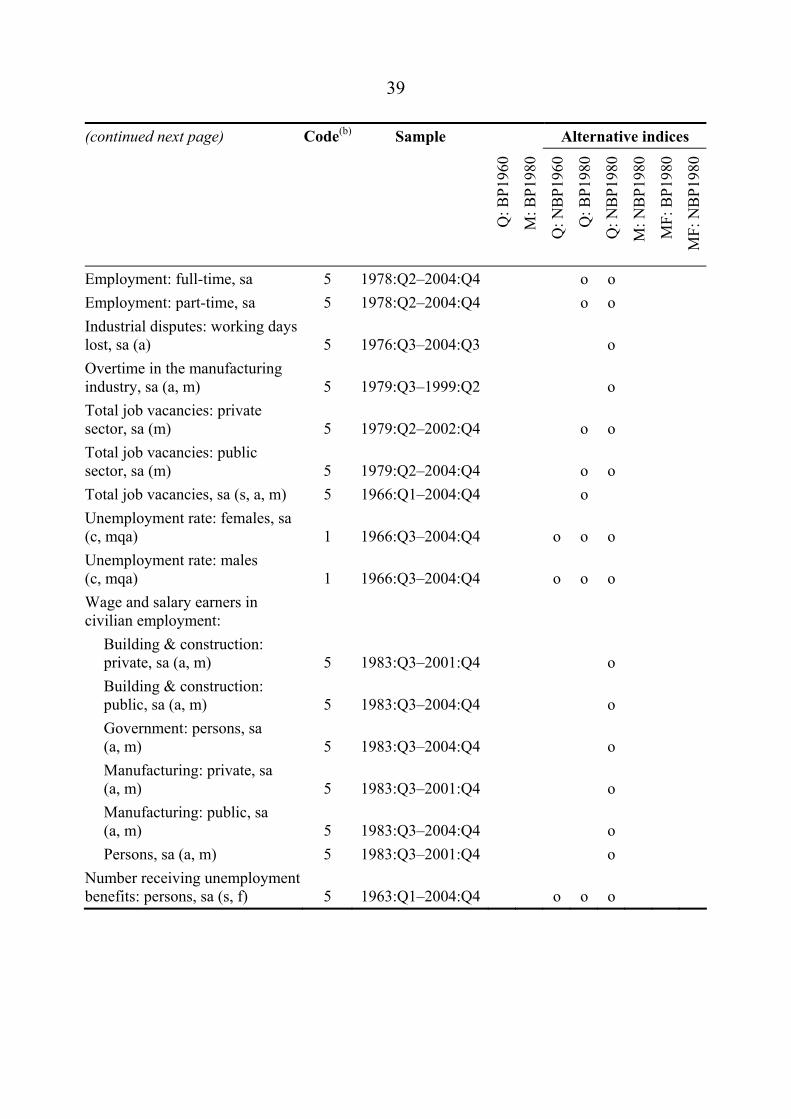
39

(continued next page) Code(b) Sample Alternative indices

Q: B

P196

0

M: B

P198

0

Q: N

BP1

960

Q: B

P198

0

Q: N

BP1

980

M: N

BP1

980

MF:

BP1

980

MF:

NB

P198

0

Employment: full-time, sa 5 1978:Q2–2004:Q4 o o Employment: part-time, sa 5 1978:Q2–2004:Q4 o o Industrial disputes: working days lost, sa (a) 5 1976:Q3–2004:Q3 o Overtime in the manufacturing industry, sa (a, m) 5 1979:Q3–1999:Q2 o Total job vacancies: private sector, sa (m) 5 1979:Q2–2002:Q4 o o Total job vacancies: public sector, sa (m) 5 1979:Q2–2004:Q4 o o Total job vacancies, sa (s, a, m) 5 1966:Q1–2004:Q4 o Unemployment rate: females, sa (c, mqa) 1 1966:Q3–2004:Q4 o o o Unemployment rate: males (c, mqa) 1 1966:Q3–2004:Q4 o o o Wage and salary earners in civilian employment: Building & construction: private, sa (a, m) 5 1983:Q3–2001:Q4 o Building & construction: public, sa (a, m) 5 1983:Q3–2004:Q4 o Government: persons, sa (a, m) 5 1983:Q3–2004:Q4 o Manufacturing: private, sa (a, m) 5 1983:Q3–2001:Q4 o Manufacturing: public, sa (a, m) 5 1983:Q3–2004:Q4 o Persons, sa (a, m) 5 1983:Q3–2001:Q4 o Number receiving unemployment benefits: persons, sa (s, f) 5 1963:Q1–2004:Q4 o o o

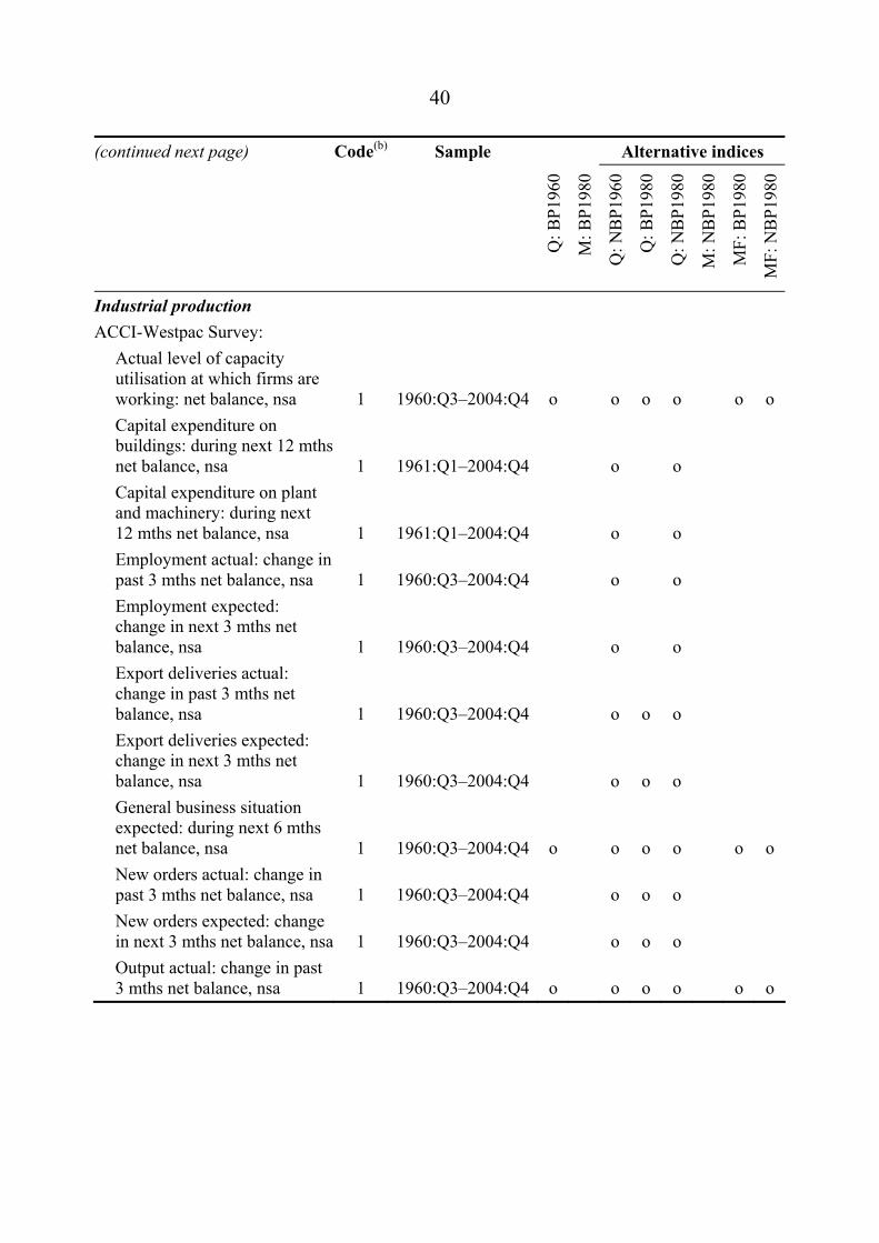
40

(continued next page) Code(b) Sample Alternative indices

Q: B

P196

0

M: B

P198

0

Q: N

BP1

960

Q: B

P198

0

Q: N

BP1

980

M: N

BP1

980

MF:

BP1

980

MF:

NB

P198

0

Industrial production ACCI-Westpac Survey: Actual level of capacity utilisation at which firms are working: net balance, nsa 1 1960:Q3–2004:Q4 o o o o o o Capital expenditure on buildings: during next 12 mths net balance, nsa 1 1961:Q1–2004:Q4 o o Capital expenditure on plant and machinery: during next 12 mths net balance, nsa 1 1961:Q1–2004:Q4 o o Employment actual: change in past 3 mths net balance, nsa 1 1960:Q3–2004:Q4 o o Employment expected: change in next 3 mths net balance, nsa 1 1960:Q3–2004:Q4 o o Export deliveries actual: change in past 3 mths net balance, nsa 1 1960:Q3–2004:Q4 o o o Export deliveries expected: change in next 3 mths net balance, nsa 1 1960:Q3–2004:Q4 o o o General business situation expected: during next 6 mths net balance, nsa 1 1960:Q3–2004:Q4 o o o o o o New orders actual: change in past 3 mths net balance, nsa 1 1960:Q3–2004:Q4 o o o New orders expected: change in next 3 mths net balance, nsa 1 1960:Q3–2004:Q4 o o o Output actual: change in past 3 mths net balance, nsa 1 1960:Q3–2004:Q4 o o o o o o

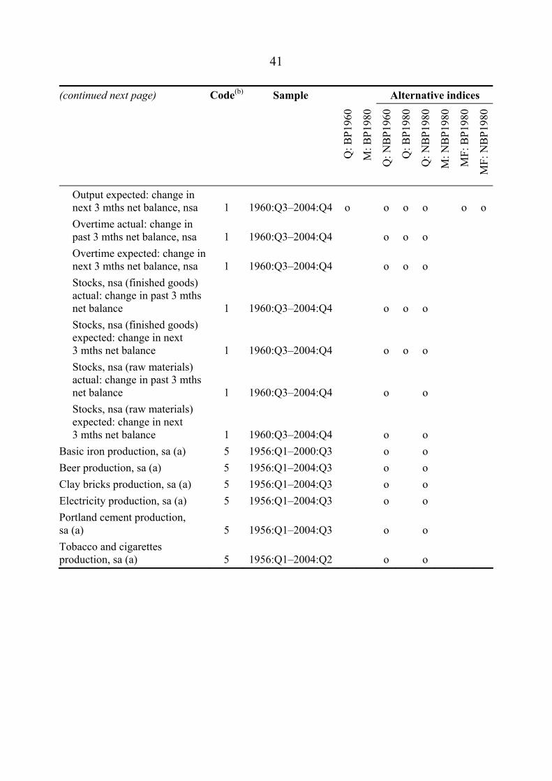
41

(continued next page) Code(b) Sample Alternative indices

Q: B

P196

0

M: B

P198

0

Q: N

BP1

960

Q: B

P198

0

Q: N

BP1

980

M: N

BP1

980

MF:

BP1

980

MF:

NB

P198

0

Output expected: change in next 3 mths net balance, nsa 1 1960:Q3–2004:Q4 o o o o o o Overtime actual: change in past 3 mths net balance, nsa 1 1960:Q3–2004:Q4 o o o Overtime expected: change in next 3 mths net balance, nsa 1 1960:Q3–2004:Q4 o o o Stocks, nsa (finished goods) actual: change in past 3 mths net balance 1 1960:Q3–2004:Q4 o o o Stocks, nsa (finished goods) expected: change in next 3 mths net balance 1 1960:Q3–2004:Q4 o o o Stocks, nsa (raw materials) actual: change in past 3 mths net balance 1 1960:Q3–2004:Q4 o o Stocks, nsa (raw materials) expected: change in next 3 mths net balance 1 1960:Q3–2004:Q4 o o Basic iron production, sa (a) 5 1956:Q1–2000:Q3 o o Beer production, sa (a) 5 1956:Q1–2004:Q3 o o Clay bricks production, sa (a) 5 1956:Q1–2004:Q3 o o Electricity production, sa (a) 5 1956:Q1–2004:Q3 o o Portland cement production, sa (a) 5 1956:Q1–2004:Q3 o o Tobacco and cigarettes production, sa (a) 5 1956:Q1–2004:Q2 o o

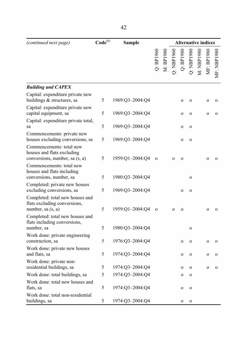
42

(continued next page) Code(b) Sample Alternative indices

Q: B

P196

0

M: B

P198

0

Q: N

BP1

960

Q: B

P198

0

Q: N

BP1

980

M: N

BP1

980

MF:

BP1

980

MF:

NB

P198

0

Building and CAPEX Capital: expenditure private new buildings & structures, sa 5 1969:Q3–2004:Q4 o o o o Capital: expenditure private new capital equipment, sa 5 1969:Q3–2004:Q4 o o o o Capital: expenditure private total, sa 5 1969:Q3–2004:Q4 o o Commencements: private new houses excluding conversions, sa 5 1969:Q3–2004:Q4 o o Commencements: total new houses and flats excluding conversions, number, sa (s, a) 5 1959:Q1–2004:Q4 o o o o o Commencements: total new houses and flats including conversions, number, sa 5 1980:Q3–2004:Q4 o Completed: private new houses excluding conversions, sa 5 1969:Q3–2004:Q4 o o Completed: total new houses and flats excluding conversions, number, sa (s, a) 5 1959:Q1–2004:Q4 o o o o o Completed: total new houses and flats including conversions, number, sa 5 1980:Q3–2004:Q4 o Work done: private engineering construction, sa 5 1976:Q3–2004:Q4 o o o o Work done: private new houses and flats, sa 5 1974:Q3–2004:Q4 o o o o Work done: private non-residential buildings, sa 5 1974:Q3–2004:Q4 o o o o Work done: total buildings, sa 5 1974:Q3–2004:Q4 o o Work done: total new houses and flats, sa 5 1974:Q3–2004:Q4 o o Work done: total non-residential buildings, sa 5 1974:Q3–2004:Q4 o o

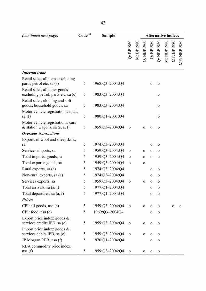
43

(continued next page) Code(b) Sample Alternative indices

Q: B

P196

0

M: B

P198

0

Q: N

BP1

960

Q: B

P198

0

Q: N

BP1

980

M: N

BP1

980

MF:

BP1

980

MF:

NB

P198

0

Internal trade Retail sales, all items excluding parts, petrol etc, sa (s) 5 1968:Q3–2004:Q4 o o Retail sales, all other goods excluding petrol, parts etc, sa (c) 5 1983:Q3–2004:Q4 o Retail sales, clothing and soft goods, household goods, sa 5 1983:Q3–2004:Q4 o Motor vehicle registrations: total, sa (f) 5 1980:Q1–2001:Q4 o Motor vehicle registrations: cars & station wagons, sa (s, a, f) 5 1959:Q3–2004:Q4 o o o o Overseas transactions Exports of wool and sheepskins, sa 5 1974:Q3–2004:Q4 o o Services imports, sa 5 1959:Q3–2004:Q4 o o o o Total imports: goods, sa 5 1959:Q3–2004:Q4 o o o o Total exports: goods, sa 5 1959:Q3–2004:Q4 o o Rural exports, sa (a) 5 1974:Q3–2004:Q4 o o Non-rural exports, sa (a) 5 1974:Q3–2004:Q4 o o Services exports, sa 5 1959:Q3–2004:Q4 o o o o Total arrivals, sa (a, f) 5 1977:Q1–2004:Q4 o o Total departures, sa (a, f) 5 1977:Q1–2004:Q4 o o Prices CPI: all goods, nsa (s) 5 1959:Q3–2004:Q4 o o o o o o CPI: food, nsa (c) 5 1969:Q3–2004Q4 o o Export price index: goods & services credits IPD, sa (c) 5 1959:Q3–2004:Q4 o o o o Import price index: goods & services debits IPD, sa (c) 5 1959:Q3–2004:Q4 o o o o JP Morgan RER, nsa (f) 5 1970:Q1–2004:Q4 o o RBA commodity price index, nsa (f) 5 1959:Q3–2004:Q4 o o o o

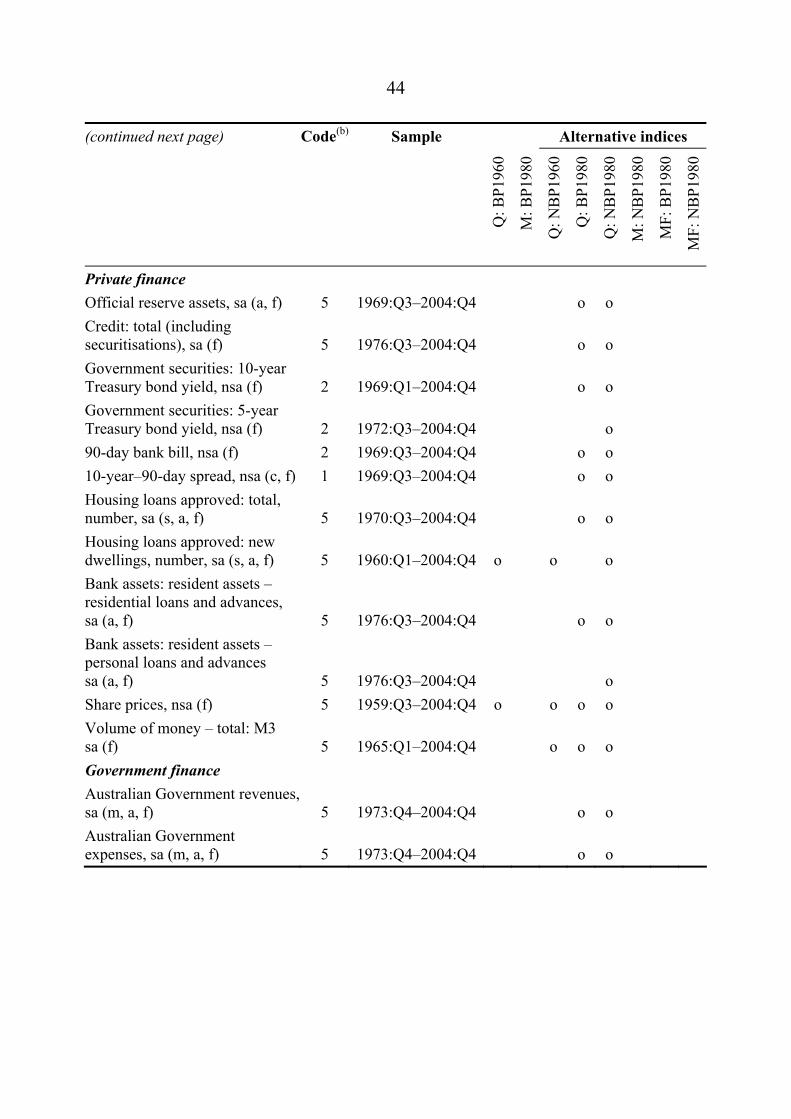
44

(continued next page) Code(b) Sample Alternative indices

Q: B

P196

0

M: B

P198

0

Q: N

BP1

960

Q: B

P198

0

Q: N

BP1

980

M: N

BP1

980

MF:

BP1

980

MF:

NB

P198

0

Private finance Official reserve assets, sa (a, f) 5 1969:Q3–2004:Q4 o o Credit: total (including securitisations), sa (f) 5 1976:Q3–2004:Q4 o o Government securities: 10-year Treasury bond yield, nsa (f) 2 1969:Q1–2004:Q4 o o Government securities: 5-year Treasury bond yield, nsa (f) 2 1972:Q3–2004:Q4 o 90-day bank bill, nsa (f) 2 1969:Q3–2004:Q4 o o 10-year–90-day spread, nsa (c, f) 1 1969:Q3–2004:Q4 o o Housing loans approved: total, number, sa (s, a, f) 5 1970:Q3–2004:Q4 o o Housing loans approved: new dwellings, number, sa (s, a, f) 5 1960:Q1–2004:Q4 o o o Bank assets: resident assets – residential loans and advances, sa (a, f) 5 1976:Q3–2004:Q4 o o Bank assets: resident assets – personal loans and advances sa (a, f) 5 1976:Q3–2004:Q4 o Share prices, nsa (f) 5 1959:Q3–2004:Q4 o o o o Volume of money – total: M3 sa (f) 5 1965:Q1–2004:Q4 o o o Government finance Australian Government revenues, sa (m, a, f) 5 1973:Q4–2004:Q4 o o Australian Government expenses, sa (m, a, f) 5 1973:Q4–2004:Q4 o o

45

(continued next page) Code(b) Sample Alternative indices

Q: B

P196

0

M: B

P198

0

Q: N

BP1

960

Q: B

P198

0

Q: N

BP1

980

M: N

BP1

980

MF:

BP1

980

MF:

NB

P198

0

Monthly Employment Employment, sa 5 1978:M2–2004:M12 o o o o Employment: full-time, sa 5 1978:M2–2004:M12 o o o o Employment: part-time, sa 5 1978:M2–2004:M12 o o o o Industrial disputes: working days lost, sa (a) 5 1976:M6–2004:M12 o o Number receiving unemployment benefits: persons, sa 5 1976:M7–2004:M12 o o o o Participation rate, sa 2 1978:M2–2004:M12 o o o o Total arrivals, sa (a) 5 1977:M1–2004:M12 o o o o Total departures, sa (a) 5 1977:M1–2004:M12 o o o o Unemployment rate, sa 2 1978:M2–2004:M12 o o o o Wage and salary earners in civilian employment: Government: persons, sa 5 1983:M1–2001:M12 o o Private: persons, sa 5 1983:M1–2001:M12 o o Building & construction: total, sa 5 1983:M1–2001:M12 o o Manufacturing: total, sa 5 1983:M1–2001:M12 o o Building and CAPEX Approvals: private new houses and flats, number, sa 5 1965:M1–2004:M12 o o Approvals: total residential buildings, value, sa (d) 5 1978:M1–2004:M12 o o o o Approvals: total new houses and flats, number, sa (s, a) 5 1959:M9–2004:M12 o o o o Approvals: total non-residential buildings, value, sa (s, a, d) 5 1978:M3–2004:M12 o o o o Internal trade Motor vehicle registrations: total, spliced to sales at 2002:M1, sa (s) 5 1980:M1–2004:M12 o o

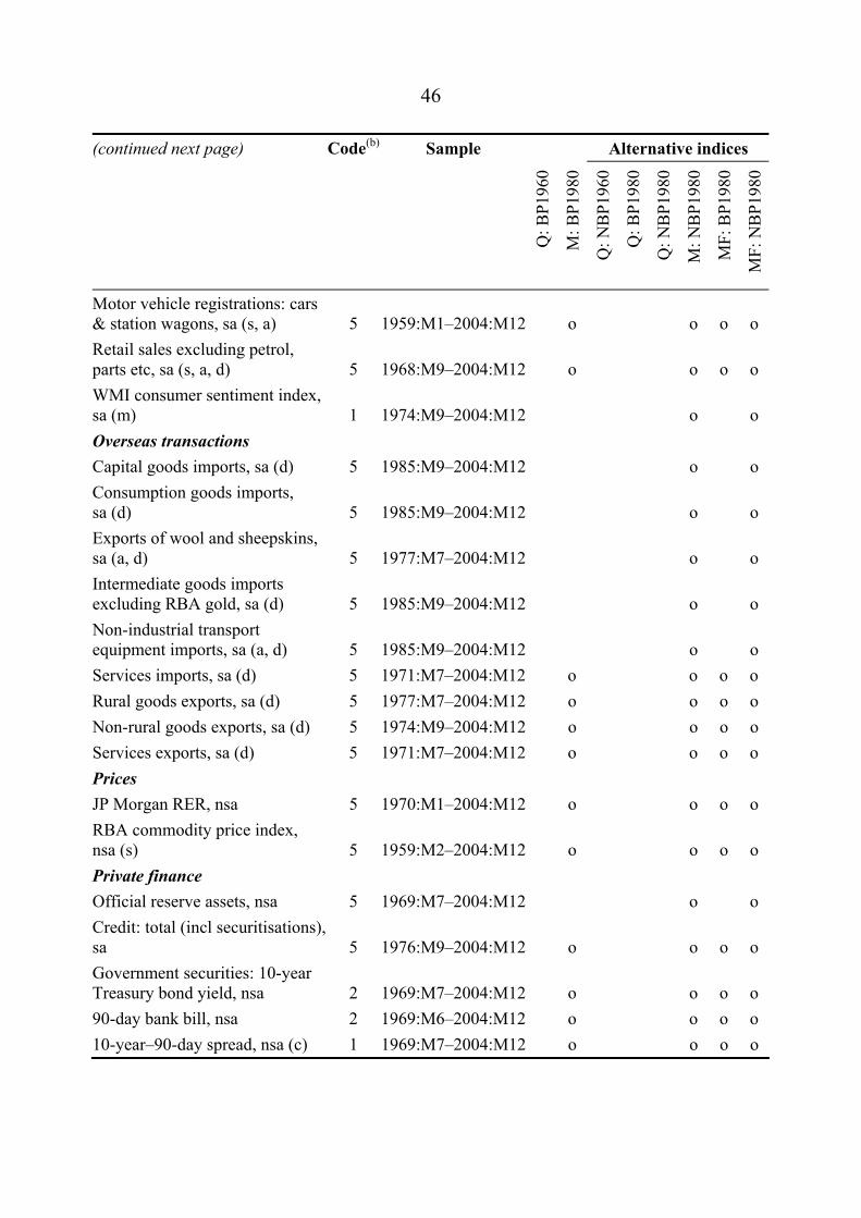
46

(continued next page) Code(b) Sample Alternative indices

Q: B

P196

0

M: B

P198

0

Q: N

BP1

960

Q: B

P198

0

Q: N

BP1

980

M: N

BP1

980

MF:

BP1

980

MF:

NB

P198

0

Motor vehicle registrations: cars & station wagons, sa (s, a) 5 1959:M1–2004:M12 o o o o Retail sales excluding petrol, parts etc, sa (s, a, d) 5 1968:M9–2004:M12 o o o o WMI consumer sentiment index, sa (m) 1 1974:M9–2004:M12 o o Overseas transactions Capital goods imports, sa (d) 5 1985:M9–2004:M12 o o Consumption goods imports, sa (d) 5 1985:M9–2004:M12 o o Exports of wool and sheepskins, sa (a, d) 5 1977:M7–2004:M12 o o Intermediate goods imports excluding RBA gold, sa (d) 5 1985:M9–2004:M12 o o Non-industrial transport equipment imports, sa (a, d) 5 1985:M9–2004:M12 o o Services imports, sa (d) 5 1971:M7–2004:M12 o o o o Rural goods exports, sa (d) 5 1977:M7–2004:M12 o o o o Non-rural goods exports, sa (d) 5 1974:M9–2004:M12 o o o o Services exports, sa (d) 5 1971:M7–2004:M12 o o o o Prices JP Morgan RER, nsa 5 1970:M1–2004:M12 o o o o RBA commodity price index, nsa (s) 5 1959:M2–2004:M12 o o o o Private finance Official reserve assets, nsa 5 1969:M7–2004:M12 o o Credit: total (incl securitisations), sa 5 1976:M9–2004:M12 o o o o Government securities: 10-year Treasury bond yield, nsa 2 1969:M7–2004:M12 o o o o 90-day bank bill, nsa 2 1969:M6–2004:M12 o o o o 10-year–90-day spread, nsa (c) 1 1969:M7–2004:M12 o o o o

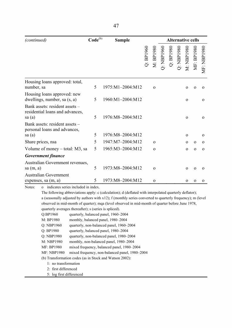
47

(continued) Code(b) Sample Alternative cells

Q: B

P196

0

M: B

P198

0

Q: N

BP1

960

Q: B

P198

0

Q: N

BP1

980

M: N

BP1

980

MF:

BP1

980

MF:

NB

P198

0

Housing loans approved: total, number, sa 5 1975:M1–2004:M12 o o o o Housing loans approved: new dwellings, number, sa (s, a) 5 1960:M1–2004:M12 o o Bank assets: resident assets – residential loans and advances, sa (a) 5 1976:M8–2004:M12 o o Bank assets: resident assets – personal loans and advances, sa (a) 5 1976:M8–2004:M12 o o Share prices, nsa 5 1947:M7–2004:M12 o o o o Volume of money – total: M3, sa 5 1965:M3–2004:M12 o o o o Government finance Australian Government revenues,sa (m, a) 5 1973:M8–2004:M12 o o o o Australian Government expenses, sa (m, a) 5 1973:M8–2004:M12 o o o o Notes: o indicates series included in index. The following abbreviations apply: c (calculation); d (deflated with interpolated quarterly deflator); a (seasonally adjusted by authors with x12); f (monthly series converted to quarterly frequency); m (level observed in mid-month of quarter); mqa (level observed in mid-month of quarter before June 1978, quarterly averages thereafter); s (series is spliced). Q:BP1960 quarterly, balanced panel, 1960–2004 M: BP1980 monthly, balanced panel, 1980–2004 Q: NBP1960 quarterly, non-balanced panel, 1960–2004 Q: BP1980 quarterly, balanced panel, 1980–2004 Q: NBP1980 quarterly, non-balanced panel, 1980–2004 M: NBP1980 monthly, non-balanced panel, 1980–2004 MF: BP1980 mixed frequency, balanced panel, 1980–2004 MF: NBP1980 mixed frequency, non-balanced panel, 1980–2004 (b) Transformation codes (as in Stock and Watson 2002): 1: no transformation 2: first differenced 5: log first differenced

48

Appendix B: Dating Recessions

In this paper, we use the Bry and Boschan (1971) algorithm to date recessions. This algorithm implements NBER-style dating of business cycle peaks and troughs in monthly data. The Gauss code to implement Bry-Boschan for monthly data was obtained from Mark Watson’s website <http://www.wws.princeton.edu/ ~mwatson/publi.html> and was used in Watson (1994). The Bry-Boschan algorithm has been applied to Australian monthly data by Boehm and Moore (1984), Boehm and Summers (1999) and Pagan (1997). We also use a variant of the Bry-Boschan algorithm to date cycles in quarterly series. A quarterly version of the Bry-Boschan algorithm has been used by many authors, including Altissimo et al (2001), Cashin and Ouliaris (2004), Harding and Pagan (2002, 2003, 2005) and Inklaar et al (2003).

The quarterly algorithm, which also serves as an intuitive analogy to the more complex monthly algorithm, is given by the following steps:

Step 1: Local peaks (troughs) in real GDP are found as quarters greater (less) than their neighbouring two quarters either side.

Step 2: Peaks (troughs) are forced to alternate by eliminating the smaller (shallower) of any two consecutive peaks (troughs).

Step 3: A minimum phase length (peak-to-peak or trough-to-trough) of five quarters is enforced. The peak or trough removed is chosen such that the average depth of recessions is greatest after removing that point.

Step 4: Peaks (troughs) that are lower (higher) than previous troughs (peaks) are eliminated by removing that trough-peak (peak-trough) phase.

Step 5: The first and last peaks (troughs) are eliminated if they are not greater (less) than the maximum (minimum) of the points at the ends of the series.

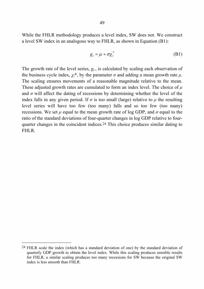
49

While the FHLR methodology produces a level index, SW does not. We construct a level SW index in an analogous way to FHLR, as shown in Equation (B1):

(B1) *ttg σχµ +=

The growth rate of the level series, gt , is calculated by scaling each observation of the business cycle index, χt*, by the parameter σ and adding a mean growth rate µ. The scaling ensures movements of a reasonable magnitude relative to the mean. These adjusted growth rates are cumulated to form an index level. The choice of µ and σ will affect the dating of recessions by determining whether the level of the index falls in any given period. If σ is too small (large) relative to µ the resulting level series will have too few (too many) falls and so too few (too many) recessions. We set µ equal to the mean growth rate of log GDP, and σ equal to the ratio of the standard deviations of four-quarter changes in log GDP relative to four-quarter changes in the coincident indices.24 This choice produces similar dating to FHLR.

24 FHLR scale the index (which has a standard deviation of one) by the standard deviation of quarterly GDP growth to obtain the level index. While this scaling produces sensible results for FHLR, a similar scaling produces too many recessions for SW because the original SW index is less smooth than FHLR.

50

Appendix C: Revisions to GDP and Recession Dating

Figure C1 shows the dating of recessions for the period 1960:Q1 to 1992:Q4 for vintages of GDP from 1971:Q1 to 2004:Q4. Recessions are shown as black bars. Looking across the figure shows which GDP vintages classified that quarter as being in recession. Looking down the figure shows the dates of recessions for a given GDP vintage. The recessions observed in 1960–1961, 1982–1983 and 1990–1991 are robust across the different vintages of GDP, although the length and precise timing of these recessions has changed with revisions to the national accounts. All vintages of GDP after 1974:Q2, with the exception of the 1998:Q3–1999:Q2 vintages, identify at least one recession in the 1970s. However, the timing of recessions in the 1970s has been subject to substantial revision. In part, this appears to be the result of larger revisions to GDP in the 1970s. Furthermore, with lower average growth in the 1970s, small revisions to GDP can easily change the dating of recessions. No recessions are found after 1992.

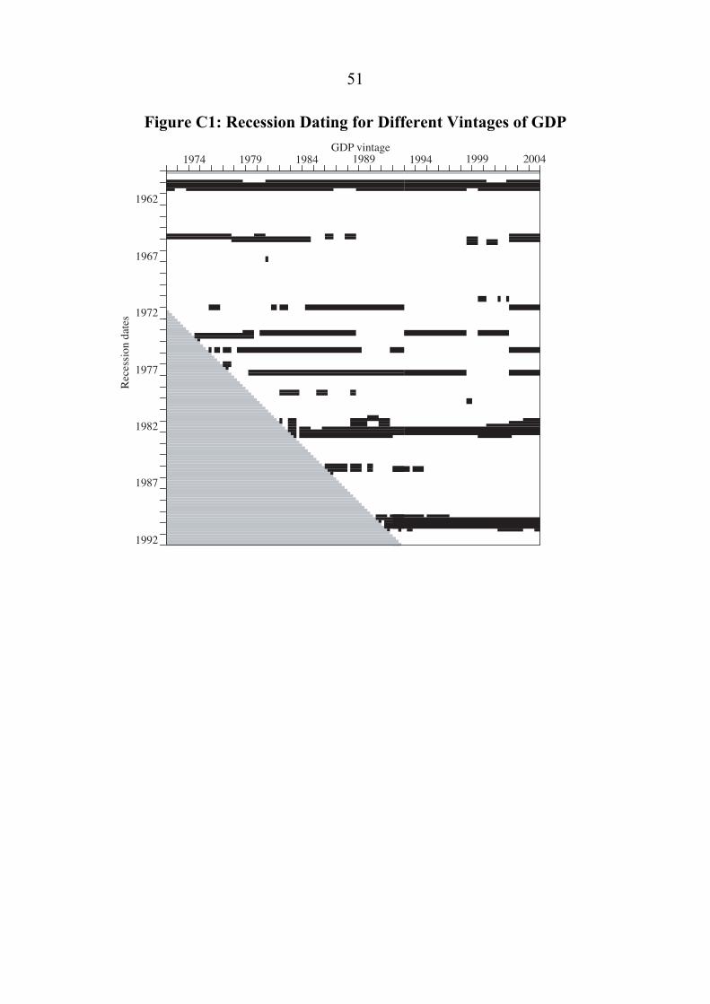
51

Figure C1: Recession Dating for Different Vintages of GDP

1992

1987

1972

1982

1967

1962

1977

19891974 1979 1984 1994 1999 2004GDP vintage

52

References

Altissimo F, A Bassanetti, R Cristadoro, M Forni, M Lippi, M Hallin, L Reichlin and G Veronese (2001), ‘EuroCOIN: a real time coincident indicator of the euro area business cycle’, Centre for Economic Policy Research Discussion Paper No 3108.

Andrews D and M Kohler (2005), ‘International business cycle co-movements through time’, in CJ Kent and D Norman (eds), The changing nature of the business cycle, Proceedings of a Conference, Reserve Bank of Australia, Sydney, pp 188–219.

Artis MJ, A Banerjee and M Marcellino (2005), ‘Factor forecasts for the UK’, Journal of Forecasting, 4, pp 279–298.

Bai J and S Ng (2002), ‘Determining the number of factors in approximate factor models’, Econometrica, 70(1), pp 191–221.

Beck MT, MG Bush and RW Hayes (1973), ‘The indicator approach to the identification of business cycles’, Reserve Bank of Australia Occasional Paper No 2, 2nd edn.

Bernanke BS and J Boivin (2003), ‘Monetary policy in a data-rich environment’, Journal of Monetary Economics, 50(3), pp 525–546.

Bernanke BS, J Boivin and P Eliasz (2005), ‘Measuring the effects of monetary policy: a factor-augmented vector autoregressive (FAVAR) approach’, Quarterly Journal of Economics, 120(1), pp 387–422.

Boehm EA and GH Moore (1984), ‘New economic indicators for Australia, 1949–84’, Australian Economic Review, 4th Quarter, pp 34–56.

Boehm EA and PM Summers (1999), ‘Analysing and forecasting business cycles with the aid of economic indicators’, International Journal of Management Reviews, 1(3), pp 245–277.

53

Boivin J and S Ng (2005), ‘Understanding and comparing factor-based forecasts’, NBER Working Paper No 11285.

Boivin J and S Ng (forthcoming), ‘Are more data always better for factor analysis?’, Journal of Econometrics.

Bry G and C Boschan (1971), ‘Cyclical analysis of time series: selected procedures and computer programs’, NBER Technical Working Paper No 20.

Burns AF and WC Mitchell (1946), Measuring business cycles, NBER, New York.

Bush MG and AM Cohen (1968), ‘The indicator approach to the identification of business cycles’, Reserve Bank of Australia Occasional Paper No 2, 1st edn.

Cashin P and S Ouliaris (2004), ‘Key features of Australian business cycles’, Australian Economic Papers, 43(1), pp 39–58.

Caton C (2005), ‘Discussion of “The Australian business cycle: a coincident indicator approach”’, in CJ Kent and D Norman (eds), The changing nature of the business cycle, Proceedings of a Conference, Reserve Bank of Australia, Sydney, pp 308–311.

Federal Reserve Bank of Chicago (2000), ‘CFNAI background release’, available at <http://www.chicagofed.org/economic_research_and_data/files/ cfnai_background.pdf>.

Federal Reserve Bank of Chicago (2003), ‘CFNAI technical report’, available at <http://www.chicagofed.org/economic_research_and_data/files/ cfnai_technical_report.pdf>.

Forni M, M Hallin, M Lippi and L Reichlin (2000), ‘The generalized dynamic-factor model: identification and estimation’, Review of Economics and Statistics, 82(4), pp 540–554.

Forni M, M Hallin, M Lippi and L Reichlin (2001), ‘Coincident and leading indicators for the euro area’, Economic Journal, 111(471), pp C62–C85.

54

Forni M, M Hallin, M Lippi and L Reichlin (2005), ‘The generalized dynamic factor model: one-sided estimation and forecasting’, Journal of the American Statistical Association, 100(471), pp 830–840.

Forni M and L Reichlin (1998), ‘Let’s get real: a factor analytical approach to disaggregated business cycle dynamics’, Review of Economic Studies, 65(3), pp 453–473.

Harding D (2002), ‘The Australian business cycle: a new view’, University of Melbourne, mimeo.

Harding D and A Pagan (2002), ‘Dissecting the cycle: a methodological investigation’, Journal of Monetary Economics, 49(2), pp 365–381.

Harding D and A Pagan (2003), ‘A comparison of two business cycle dating methods’, Journal of Economic Dynamics and Control, 27(9), pp 1681–1690.

Harding D and A Pagan (2005), ‘A suggested framework for classifying the modes of cycle research’, Journal of Applied Econometrics, 20(2), pp 151–159.

Haywood E (1973), ‘The deviation cycle: a new index of the Australian business cycle 1950–1973’, Australian Economic Review, 4th Quarter, pp 31–39.

Inklaar R, J Jacobs and W Romp (2003), ‘Business cycle indexes: does a heap of data help?’, University of Groningen, CCSO Working Paper No 2003/12.

Pagan A (1997), ‘Towards an understanding of some business cycle characteristics’, Australian Economic Review, 30(1), pp 1–15.

Reserve Bank of Australia (RBA) (1997), Semi-annual statement on monetary policy, May.

Simon J (2001), ‘The decline in Australian output volatility’, Reserve Bank of Australia Research Discussion Paper No 2001-01.

Stock JH and MW Watson (1999), ‘Forecasting inflation’, Journal of Monetary Economics, 44(2), pp 293–335.

55

Stock JH and MW Watson (2002a), ‘Forecasting using principal components from a large number of predictors’, Journal of the American Statistical Association, 97(460), pp 1167–1179.

Stock JH and MW Watson (2002b), ‘Macroeconomic forecasting using diffusion indexes’, Journal of Business and Economic Statistics, 20(2), pp 147–162.

Watson MW (1994), ‘Business-cycle durations and postwar stabilization of the U.S. economy’, American Economic Review, 84(1), pp 24–46.

Watson MW (2001), ‘Macroeconomic forecasting using many predictors’, in M Dewatripont, LP Hansen and SJ Turnovsky (eds), Advances in economics and econometrics: theory and applications, Eighth World Congress, Volume III, Cambridge University Press, Cambridge, pp 87–114.