five algorithms to optimize and correct the tool path of

1

Five Algorithms to Optimize and Correctthe Tool Path of the Five-Axis Milling Machine

S.S. Makhanov and M. MunlinDepartment of Information Technology,

Sirindhorn International Institute of Technology, Thammasat University, Pathum Thani, 12121, Thailand

[email protected]

www.5axis-thai.com

Two Royal Golden Jubilee Scholarships of the Thailand Research Fund are available for Thai Master of Ph.D. students

2

Cutter

CutterTilt Table

Rotary TableWorkpiece

Milling Machines Maho600E and HERMLE

Cutter Rotary Table

Tilt Table

Rotary Table

Tilt Table

3

5-Axis Machining

4

CAD

NCprogram

General Objective: Tool path Optimization. A Software Prototype Tool path OptimizerCriteria: kinematics error, scallop height, machining stripAdaptive tool paths(grids, space filling curves, angle optimization) Gouging avoidance, Collision detection

Tool pathInverse

kinematicsModeling

kernel

Error estimator 1with visualization

Tool tip errorScallop height

Gouging Machining strip

Solid model of the machine

Visual collision detection

Error estimator 2and visualizationMaterial removalintegrated with

the UG

Virtual Milling Machine

Errors

NURBS(IGES)

Tool path

5

Optimization Problem Given a surface find a set of tool positions and orientationssuch that the surface is cut with max accuracy for minimum time

6

Idea 1. Curvilinear grids

(a) (b)

Adaptation of the spiral tool path. Grid in the polar coordinates

8

High accuracy milling

A very high density of the CL- points

Enter the circular region

Start the spiral motion

Exit from the circular regionComposite patterns

Adaptation to the boundary & pockets

Robot with sad face Oister

11

A complicated boundary & a pocket

12

Workpeices produced by means of adaptive tool path

Concave-convex surface, plastic

Parabolic surface, wood

Concave-convex Beziersurface, steel

Concave-convex surface, wood

Complex boundary,wood

Internal boundary, wood.

13

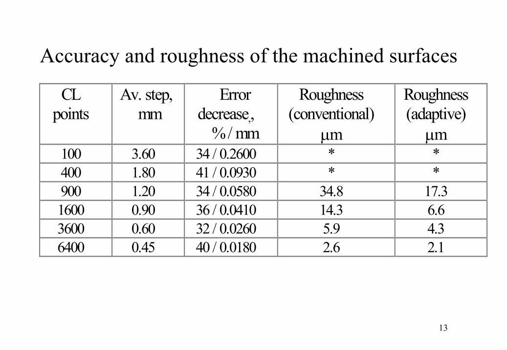
CLpoints

Av. step,mm

Errordecrease,,

% / mm

Roughness(conventional)

µm

Roughness(adaptive)

µm100 3.60 34 / 0.2600 * *400 1.80 41 / 0.0930 * *900 1.20 34 / 0.0580 34.8 17.31600 0.90 36 / 0.0410 14.3 6.63600 0.60 32 / 0.0260 5.9 4.36400 0.45 40 / 0.0180 2.6 2.1

Accuracy and roughness of the machined surfaces

14

Idea 2. Space-Filling Curve

• SFC is a continuous mapping of a unit line segment onto the unit square.

15

Adaptive Space-Filling Curve Construction

• Overlay two iso-parametric tool paths; one in the v-direction and one in the u-direction.

Iso-parametric tool path in v-direction

Iso-parametric tool path in u-direction

The resulting grid

16

Machining strip must cover the entire surface

17

Space-Filling Curve Generation

• Generation of space-filling curve is formulated as the Hamiltonian path problem.

• The grid is first covered by small rectangular circuits.

18


• Any two adjacent circuits merge into a bigger circuit. The cost of merging is defined as:

Where |e| presents the length (distance) of the edge e.• Define a dual graph G’:

Each small circuit in G defines a vertex in G’Two edges connecting two small circuits in G define an edge in G’

A B

C

D

e fs

tA′ B′

C′

D′

v′

fetsBACost −−+=),(

Dual Graph G’

19


• Merging is done by constructing a minimum spanning tree on the dual grid graph

• Tool path is obtained by removing virtual edges (dashed line), if any.

Minimum Spanning Tree of Dual Graph G’

Corresponding Hamiltonian Path In G

20

Tool Path Correction

21

Example 1

22

Example 1 Machining

Cutting without tool path correction Cutting with tool path corrections

23

Example 2

24

Example 3

The Unigraphis Simulator

25

6780.847955.582637.54SFC tool path

9036.179397.972648.12Iso-parametric in the u-direction

7831.709397.973917.31Iso-parametric in the v-direction

Example 3Example 2Example 1

Total path length (mm)Tool Path

Efficiency of the SFC tool path

26

Calculate optimal directions. Find clusters of the optimal directions which “look like” zigzag or spiral

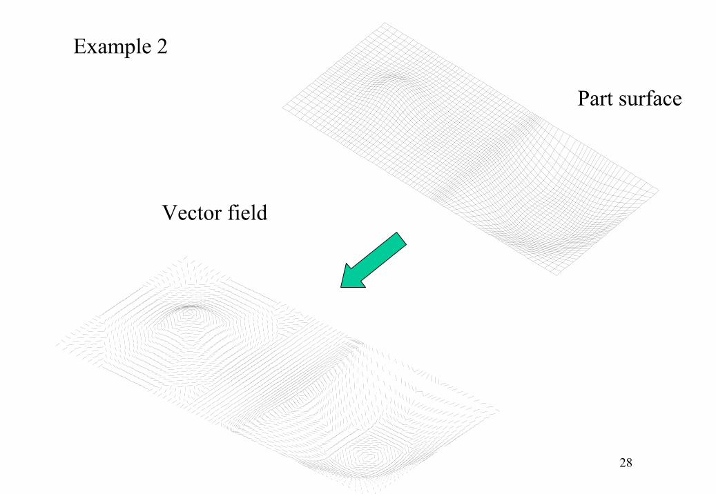
Idea 3. Vector Field Clustering

f

Fy Fx−,( )

27

Part surfaceTool path

Machining

K –means/ Normalized cut method/ DBSCAN

Vector field analysis

28

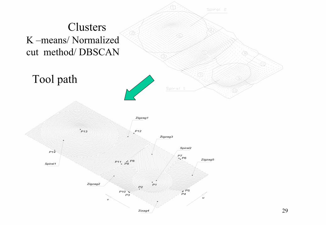
Example 2

Part surface

Vector field

29

Clusters

Tool path

K –means/ Normalized cut method/ DBSCAN

30

Example 2Actual machining

Comparison between tool path calculated by the proposed method and by the iso-parametric method

15220616.16The vdir

29620255.37The udirConventional

Method

30018675.45Vector Field

Number of turnsCC path length

(mm)

31

Idea 4. Angle Optimization

32

Around or across the hill ? The first rotary axis

The second rotary axis

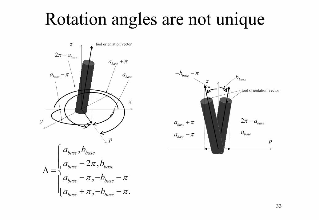
33

tool orientation vector

baseabasea π−basea π+ 2 baseaπ −

p

zbaseb π− −

baseb

tool orientation vector

baseabasea π−

basea π+2 baseaπ −

x

y

z

p

,2 ,

,, .

base base

base base

base base

base base

a ba ba ba b

ππ ππ π

−Λ = − − − + − −

Rotation angles are not unique

34

The Shortest Path

,1basea

,1baseb

,2basea π−,2baseb π− −

,2basea π+

,2baseb π− −

,2basea

,2baseb

,22 baseaπ−

,2baseb

,3basea π−,3baseb π− −

,3basea π+

,3baseb π− −

,3basea

,3baseb

,32 baseaπ−,3baseb

35

The shortest path for 2 points

Error Reduction 98.25%=

.7291571.1,896.0,571.1

,:After

.412.1,4.712,896.0,571.1

:Before

22

11

,2222

22

11

.,baba

bbaa

baba

−=−=′−=−=

−−=′+=′

−=−=−=−=

ππ

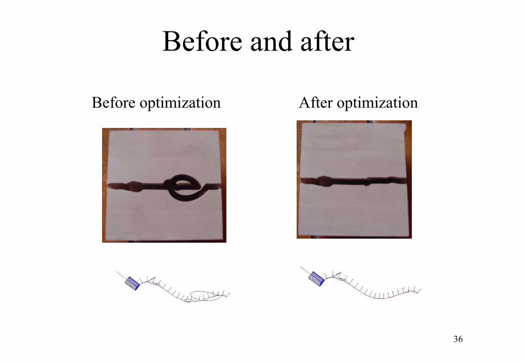
36

Before and after

Before optimization After optimization

37

Before and After

38

Efficiency

1876.49 / 1876.4903.999 3.999 130 x 201916.1/ 1911.24.07.103 7.395 100 x 202069.3 / 2020.121.06.878 8.711 40 x 202183.6 / 2038.356.07.162 16.253 30 x 202367.6 / 2101.262.67.558 20.228 20 x 202500.3 / 2123.055.98.517 19.300 15 x 202825.6 / 2255.547.912.426 23.862 10 x 20

Path lengthNon-opt/opt(mm)

error decrease(%)

Optimizationmax error (mm )

No optimization max error(mm)

Tool path

39

Impeller before and after

40

Idea 5. The error depends the on workpiece initial orientation

and the machine setup

41

Least Square Error

12

, 1 , 101

2 2 2, 1 , 1 , 1 , 1 , 1 , 1

0

,

( ) ( ) ( ) .

Dp p p p

p

D D Dp p p p p p p p p p p p

p

W W dt

x x y y z z dt

ε + +

+ + + + + +

= −

= − + − + −

∑∫

∑∫

42

System of nonlinear Equations

• Differentiate the error function with respect to workpiece (Ra,Rb,T12),

• Solved by Newton Method.

2 2 2

2a 12

2 2 2

212

2 2 2

212 12 12

d d dd d d d d

d d dd d d d d

d d dd d d d d

a b a

a b b b

a b

R R R R T

JR R R R T

R T R T T

ε ε ε

ε ε ε

ε ε ε

=

The Jacobian matrix for the case Ra,Rb,T12

43

Example 1 Tool Path


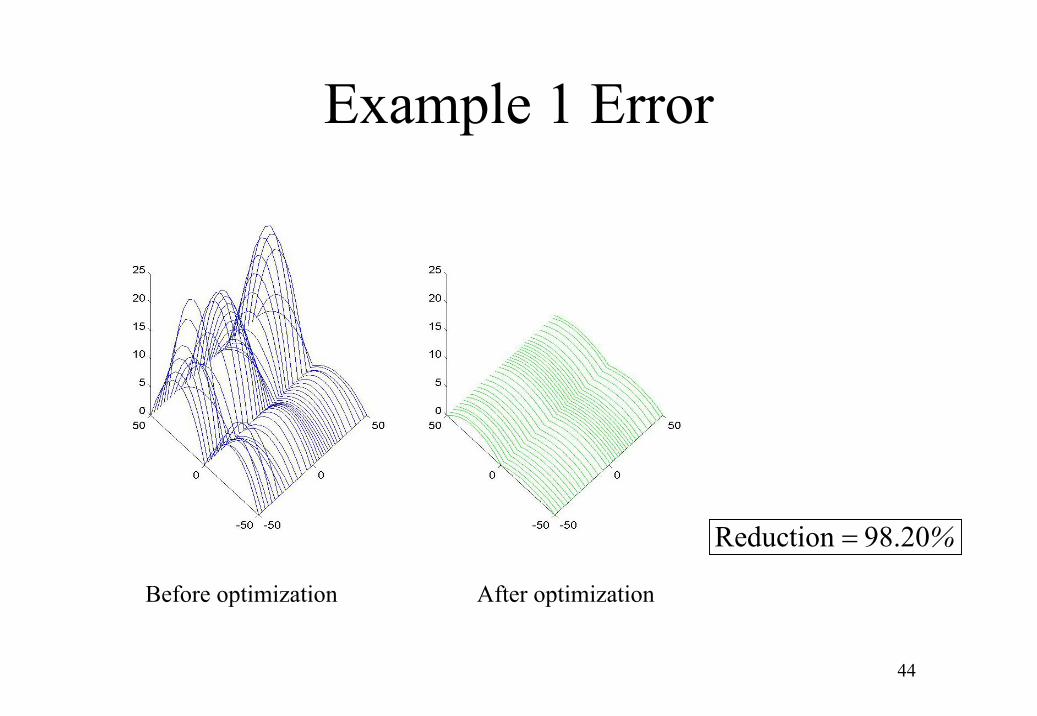
44

Example 1 Error


Reduction 98.20%=

45

Other machines Similar resultsThe 1-1 machine The 0-2 machine

46

Example 2. The 1-1 Machine


47

Example 2. The 1-1 Machine

Before optimizationReduction 98.03%=

After optimization

48

We obtained a rigorous mathematical proof that every

machine has 6 optimizable variables

The 0-2 machine

The 1-1 machine

none The 2-0 machine

Machine settings Tool Workpiece

setup Machine Type

12, 12, 12,, , , ,a b x y zr r T T T

12, 12,, , ,a b x yr r T T

,a br r

23,xT

4,zT

4,zT

34,xT

23, 23, 34,, ,x y yT T T

49

Other parameters are either invariant parameters

(The parameter doesn’t affect the tool trajectory. For example: the tool length for the 2-0 machine)

d 0dvε≡

50

or dependent variables

12, 23, cz zT T+ =

13, czT =

51

Efficiency

Surface 1Surface 2

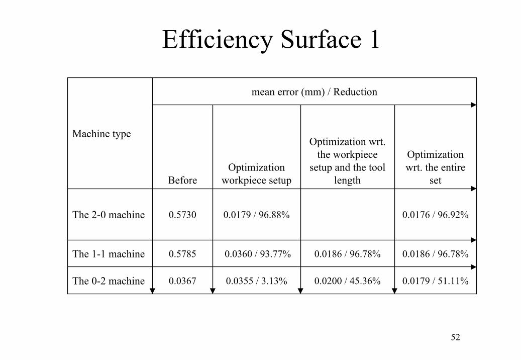
52

Efficiency Surface 1

0.0179 / 51.11%0.0200 / 45.36%0.0355 / 3.13%0.0367The 0-2 machine

0.0186 / 96.78%0.0186 / 96.78%0.0360 / 93.77%0.5785The 1-1 machine

0.0176 / 96.92%0.0179 / 96.88%0.5730The 2-0 machine

Optimization wrt. the entire

set

Optimization wrt. the workpiece

setup and the tool length

Optimization workpiece setupBefore

mean error (mm) / Reduction

Machine type

53

Efficiency Surface 2

0.1087 / 80.45%0.1220 / 78.06%0.5495 / 1.18%0.5561The 0-2 machine

0.3029 / 57.30%0.3072 / 56.68%0.6335 / 10.68%0.7092The 1-1 machine

0.1102 / 79.62%0.1118 / 79.33%0.5408The 2-0 machine

Optimization wrt. the entire

set


setup and the tool length


setup

Before optimizatio

n

mean error (mm) / Reduction

Machine type

54

Efficiency. Point Reduction

5544 / 30.0%7925Surface 2

1233 / 68.4%3900Surface 1

Optimization wrt. ra and rbBefore optimization

# of CC points / Reduction

Surface

55

Machining. The 2-0 machine. Surface 1 Before and After

56

ConclusionsWe proposed and analyzed 5 methods to optimize five-axis

machining1) Curvilinear grid techniques (30-40%) accuracy increase2) Space filling curve 10-30% tool path length decrease3) Vector field clustering 10-20% tool path length decrease 4) The shortest path minimization with regard to the angles up

to 90% accuracy increase for rough cut5) The Least square minimization with regard to the initial

position, orientation of the workpeice and configuration of the machine up to 90% accuracy increase. 30-60% decrease in the number of points (positions)

57

Associate Professor, Dr. S. S MakhanovSIIT, Thammasat

Assistant Professor Dr. M. Munlin

SIIT, Thammasat

Associate Professor, Ir. E. Bohez

School of Advanced Technologies,

AIT

Mr. W. AnotaipaiboonPh.D. Student

SIIT,Thammasat the Golden Royal Scholarship, TRF

A New Software for 5-axis Machining, Optimization, Simulation, and VerificationResearch Team

Research Assistant Mr. Than LinCIM Lab Manager, AIT

Mr. Somchai Thaopanich, Maho 600 Supervisor,

AIT

Industry CAD/CAM file formats compatibility

ME expertize,UG

ExperimentsSoftware engineering

Visualization , Solid ModelingOptimization,

Grid Generation

Solid ModelingPart time programmers (2-3 months)

UG,machining

machiningMaster student (vacant)

With the TA-ship Two Royal Golden Jubilee Scholarships of the Thailand Research

Fund are available for Thai Master of Ph.D. students

Details: www.5axis-thai.com

five algorithms to optimize and correct the tool path of

Documents