Fiscal Rules and Sovereign Default

Laura Alfaro Fabio Kanczuk

Working Paper 16-134

Working Paper 16-134

Copyright © 2016 by Laura Alfaro and Fabio Kanczuk

Working papers are in draft form. This working paper is distributed for purposes of comment and discussion only. It may not be reproduced without permission of the copyright holder. Copies of working papers are available from the author.

Fiscal Rules and Sovereign Default Laura Alfaro Harvard Business School

Fabio Kanczuk Universidade de São Paulo

Fiscal Rules and Sovereign Default*

Laura Alfaro Harvard Business School and NBER

Fabio Kanczuk Universidade de São Paulo

October 2016

Abstract

We provide a quantitative analysis of fiscal rules in a standard model of sovereign debt accumulation and default modified to incorporate quasi-hyperbolic preferences. For reasons of political economy or aggregation of citizens’ preferences, government preferences are present biased, resulting in over-accumulation of debt. Calibrating this parameter with values in the literature, the model can reproduce debt levels and frequency of default typical of emerging markets even if the household impatience parameter is calibrated to local interest rates. A quantitative exercise calibrated to Brazil finds welfare gains of the optimal fiscal policy to be economically substantial, and the optimal rule to not entail a countercyclical fiscal policy. A simple debt rule that limits the maximum amount of debt is analyzed and compared to a simple deficit rule that limits the maximum amount of deficit per period. Whereas the deficit rule does not perform well, the debt rule yields welfare gains virtually equal to the optimal rule.

JEL classification: F34, H63. Key words: sovereign debt, hyperbolic discounting, fiscal rules.

* lalfaro@hbs.edu. Harvard Business School, Boston, MA 02163, Tel: 617-495-7981, Fax: 617-495-5985; kanczuk@usp.br. Department of Economics, Universidade de São Paulo, Brazil. We thank Luis Catão, Davide Debortoli, Teresa Lloyd-Braga, Ricardo Sabbadini, Jesse Schreger, Hernán Daniel Seoane and participants at the Inflation Targeting Conference, Bank of Spain’s and Barcelona Graduate School of Economics Fiscal Sustainability in the XXI century conference, the Brazilian Central Bank seminar, DRCLAS Latin American Seminar series for valuable comments and suggestions.

2

1 Introduction

Recurrent concerns over debt sustainability in emerging markets and the ongoing European

debt crisis have prompted renewed debate in academic and policy circles on the role of fiscal rules.

A data set compiled by the Fiscal Affairs Department of the IMF identifies countries’

adoption of fiscal policy restrictions.1 Only five countries had fiscal rules in place in 1990, more

than 80 by 2014. National fiscal rules are most commonly responses to pressure on public finances.

Adoption in emerging economies was typically motivated by debt excesses resulting from the debt

crises of the 1980s and banking and economic crises in the 1990s. Rules enacted in response to the

more recent global financial crisis attempt to provide credible commitment to long-term fiscal

discipline.

Fiscal rules also play a role in business cycle frequencies. Standard economic theory holds

that fiscal policy should be countercyclical (Barro, 1979), yet most emerging countries, possibly

owing to limited access to credit markets (Bauducco and Caprioli, 2014) or distorted political

incentives (Alesina and Tabelini, 2008), follow pro-cyclical fiscal policies, which tends to

exacerbate already pronounced cycles (Kaminsky, Reinhart and Vegh, 2005; Vegh and Vuletin,

2012). Governments may adopt fiscal rules that constrain their behavior in order to correct

distorted incentives to overspend, particularly in good times. This, in turn, would alleviate distress

on rainy days.

In this paper, we examine, in the context of sovereign debt and default, the welfare

implications of fiscal rules. Despite widespread use, less research has been devoted to

understanding the optimality and role of such rules in preventing sovereign default. Are the welfare

gains of fiscal rules significant? Are the costs of limited flexibility important? Should such rules

1 See www.imf.org/external/datamapper/FiscalRules and Schmidt-Hebbel, K. and R. Soto (2006) for recent empirical analysis.

3

take into account the economic cycle? How do the welfare implications compare between simple

and sophisticated rules?

We transform the traditional model of sovereign debt and default by assuming

governments’ preferences to be time inconsistent. Specifically, our formulation of government

preferences corresponds to the quasi-hyperbolic consumption model (Laibson, 1997). The

consequent conflict between today’s government and tomorrow’s generates an incentive to pre-

commit to a particular fiscal rule. We reconcile the impatience of a government with its citizens by

recalling Jackson and Yariv (2014, 2015), who propose that aggregating citizen’s time-consistent

preferences naturally results in time-inconsistent preferences. Even if benevolent ex-ante, the

sovereign thus ends up with preferences that display an extra discount parameter that captures the

ex-post present-bias. Alternatively, a deficit bias may also emerge as an outcome of political game

as in Aguiar and Amador (2011). This argument is the primary motivator of our use of time-

inconsistent government preferences.

A second, more technical motivation relates to a problem in the calibration of models of

sovereign debt. As documented in the literature (Reinhart and Rogoff, 2009), emerging countries

are able, despite repeatedly defaulting, to accumulate debt levels close to 60% of GDP. To obtain

the observed levels of debt and default in an artificial economy, the intertemporal discount

parameter must be calibrated to extremely low numbers. Aguiar and Gopinath (2006), Alfaro and

Kanczuk (2005, 2009), and Arellano (2008) employ for annual data, beta values between 0.40 and

0.80, values much lower than that would be obtained if calibration were to local interest rates.

Notwithstanding this unintuitive calibration, the government is assumed to be benevolent and to

maximize household preferences. The use of inconsistent time preferences by the government

removes this calibration restriction allowing the household impatience parameter to be calibrated

to the interest rate.

4

Calibrating the model to the Brazilian economy, a typical emerging economy, yields the

following results. First, if the government is assumed to have hyperbolic preferences, and

calibrating this parameter with values in the literature (Angeletos et al., 2001), the model can

reproduce the Brazilian level of debt and frequency of default even if the household impatience

parameter is calibrated to local interest rates. Second, adoption of the optimal fiscal rule implies

substantive welfare gains relative to the absence of a rule. Third, the optimal fiscal rule does not

entail a countercyclical fiscal policy, as is usually believed. Fourth, under the optimal fiscal rule,

the country would never opt to default on its debt. Fifth, a simple deficit rule that sets the

maximum amount of deficit per period incurs welfare losses relative to no rule. Sixth, welfare

gains are similar between a simple debt rule that sets the maximum amount of debt and the optimal

fiscal rule. Given its simplicity and ease of contractibility, the simpler fiscal rule seems the best

option for emerging countries.

The hypothesis that governments benefit from borrowing and thus have a motive to hold

positive amounts of debt is essential to our results. This is the case of emerging countries, which

will eventually catch up to developing ones. Given that our analysis shows the benefits from front-

loading household consumption to be quantitatively more important than those from consumption

smoothing, fiscal rules should be designed to allow consumption front loading and avoid the cost

of defaults. Since there are many political economy motivations for excessive indebtedness

including common pool problem-externalities that lead to a deficit bias, and interest groups,2 we

also contrast the results to the case of a non-benevolent sovereign.

This paper relates to the vast literature on sovereign debt and default (see Amador and

Aguiar (2015) for a recent survey of the literature). In a related paper, Hatchondo et al. (2015),

study the role of sovereign default and fiscal rules limiting the maximum sovereign premium due

to the time-inconsistency of debt dilution. Differently from their work, in our model government 2 See Alesina and Drazen (1991) and Persson and Svensson (1989). See Alesina (2015) for a recent review of the literature.

5

preferences display a present bias, which creates a natural alternative role for fiscal rules. More

generally, this paper is related to a recent literature on rules versus discretion in self-control

settings (Amador, Werning and Angeletos, 2006; Halac and Yared, 2014, 2015). If fiscal rules

cannot define policy instructions for every possible shock or eventuality, there is a cost from lack

of flexibility and some discretion can be optimal. Differently from this literature, we explicitly

consider the possibility of default and its effect on debt accumulation. We also assume the private

sector to know as much as the government about the state of the economy.

The rest of the paper is organized as follows. The model is developed in Section 2 and

calibrated in Section 3. Results are reported in section 4, discussion and robustness exercises

presented in Section 5. Section 6 concludes.

2 Model

Our economy is populated by a benevolent government (the sovereign) that borrows from a

continuum of risk-neutral investors. Endowment being risky, the government may optimally

choose to default on its commitments to smooth consumption. As in Aguiar and Gopinath (2006),

Alfaro and Kanczuk (2005), and Arellano (2008), default is assumed to temporarily exclude the

government from borrowing and the sovereign incurs in additional output costs. Our environment

is thus quite similar to standard sovereign debt models. What is novel is the assumption of quasi-

hyperbolic preferences.

In more precise terms, we assume the sovereign’s preferences to be given by

(1)

with , (2)

⎥⎦

⎤⎢⎣

⎡+= ∑

∞

=+

1

)()(τ

ττδβ tttt guguEU

)1(1)(

1

σ

σ

−−=

−ggu

6

where E is the expectation operator, g denotes government consumption (or public spending), σ >

0 measures the curvature of the utility, and δ ∈ (0, 1) and β ∈ (0, 1) are the traditional discount

factor and an additional discount parameter, respectively.

Note that, the discount function being a discrete time function with values {1, βδ, βδ2, βδ3,

...}, these preferences are dynamically inconsistent in the sense that preferences at date t are

inconsistent with preferences at date (t + 1). This function, as Laibson (1997) explains, has the

advantage of mimicking the qualitative property of the hyperbolic discount function while

maintaining analytical tractability, and has been proposed, moreover, by economists and

psychologists as a characterization of human behavior.

One motivation for using such preferences in our set up is that government preferences are

an aggregation of citizens’ preferences. As Jackson and Yariv (2014, 2015) show, with any

heterogeneity in preferences, every non-dictatorial aggregation method that respects unanimity

must be time inconsistent even if citizens' preferences are time consistent. Moreover, any such

method that is time separable must entail a present bias. We can thus interpret the β < 1 parameter

as the bias resulting from this aggregation.

If the government chooses to repay its debt, its budget constraint is given by

, (3)

where dt denotes the government debt level in period t , τ is the exogenous and constant tax rate,

and zt is the technology state that determines the output level, exp(zt), in the present period. The

debt price functions, q(st, dt+1), are endogenously determined in the model and potentially depend

on all the states of the economy, st, as well as the government’s decisions.

We assume the technology state zt can take a finite number of values and evolves over time

according to a Markov transition matrix with elements π (zi , zj ). That is, the probability that zt +1 =

zj given that zt = zi is given by the matrix π element of row i and column j.

1)exp( ++−= ttttt dqdzg τ

7

When the government chooses to default, the economy’s constraint is

(4)

where the parameter ϕ governs the additional loss of output in autarky, a common feature in

sovereign debt models.3 After defaulting, the government is temporarily excluded from issuing

debt. We assume θ to be the probability that it regains full access to credit markets.

Investors are risk neutral, their opportunity cost of funds given by ρ, which denotes the

risk-free rate. The investor action is to choose the debt price qt, which depends on the perceived

likelihood of default. For investors to be indifferent between the riskless asset and lending, it must

be the case that

(5)

where ψt is the probability of default, endogenously determined and dependent on the government

incentive to repay debt.

We intentionally do not specify whether investors are international or domestic. Therefore,

dt stands for total, domestic and international, government debt level. The assumption that

investors are risk neutral implies that investors compete away their profits (and thus do not affect

the government’s utility). Another implicit assumption is that households’ private consumption

does not affect the utility they derive from public expenditures, which occurs, for example, when

the two types of consumption are separable in households’ preferences.

The timing of decisions is as follows. The government begins each period with debt level dt

and receives tax revenue endowment τexp(zt). Taking the bond price schedule q(st,dt+1) as given,

the government faces two decisions, (i) whether to default, and if it decides not to default, (ii) the

next level of debt, dt+1.

3 To keep matters simple, we assume these output costs are a constant fraction of output. Alternative costs specifications as well the addition of elements of political uncertainty, debt maturity and renegotiation have been shown to be useful ways to increase the amount of debt in equilibrium, see discussion in Mendoza and Yue (2012).

)exp()1( tt zg φτ −=

)1()1(

ρψ+−

= ttq

8

The model described is a stochastic dynamic game played by a large agent (the

government) against many small agents (the continuum of investors). We focus exclusively on the

Markov perfect equilibria, in which the sovereign (government) is not committed and players act

sequentially and rationally. This definition of equilibrium is identical to that of Arellano (2008)

and Alfaro and Kanczuk (2009), among many others, the only difference being that it was adapted

to deal with the time inconsistency problem that results from the sovereign’s preferences. The

quasi-hyperbolic assumption implies that the solution can nevertheless be written as a recursive

problem.

Note that investors are passive and their actions can be completely described by equation

(5). To write the government problem recursively, let wG denote the value function if the

government decides to maintain a good credit history (G stands for good credit history), and wB the

value function if the government defaults (B stands for bad credit history) in the present period.

The value of a good credit standing at the start of a period can then be defined as,

(6)

This indicates that the government defaults if wG < wB. The “good credit” value function wG and

policy function DG can be written as

𝑤! 𝑠! = 𝑀𝑎𝑥 𝑢 𝑔! + 𝛽𝛿𝐸𝑣 𝑠!!! (7a)

𝐷! 𝑠! = 𝐴𝑟𝑔𝑀𝑎𝑥 𝑢 𝑔! + 𝛽𝛿𝐸𝑣 𝑠!!! (7b)

subject to (3). The “bad credit” value function wB can be written as

𝑤! 𝑠! = 𝑢 𝑔! 𝛽𝛿[𝜃𝐸𝑣 𝑠!!! + 1− 𝜃 𝐸𝑣! 𝑠!!! ] (8)

subject to (4). In its turn, the “good credit” continuation value vG is written as

vG(st) = u(gt )+δEvG(st+1) (9)

subject to (3) and to

},{ BG wwMaxw =

9

. (10)

That is, it is evaluated using the policy function obtained in the good credit optimization.

The “bad credit” continuation value vB is written as

(11)

subject to (4). And the continuation value at the start of the period (with good credit standing) is

𝑣 = 𝑀𝑎𝑥{𝑣! , 𝑣!} (12)

To compute the equilibrium, it is useful to define a default set of states of the economy in

which the government chooses to default. The default set, in turn, determines the price qt through

expression (5). With these prices, one can solve the government problem (7) to (11). The solution

for (6) determines the default set, which can be used in the next iteration.

The recursive equilibrium is defined by the set of policy functions for government asset

holdings and default choice such that (i) taking the price functions as given, the government policy

functions satisfy the government optimization problem, and (ii) the price of bonds is consistent

with the government decisions.

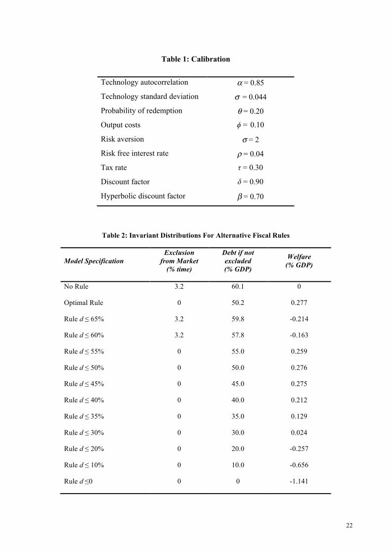
3 Calibration

We calibrate the model to Brazilian annual data from 1955. Brazil is a relatively large and

typical Emerging economy. Its sovereign debt level, frequency of default and Business Cycle

characteristics are similar to those of Mexico, for example.

We set the risk-free (international) interest rate ρ = 0.04 and inter-temporal substitution

parameter σ = 2, as is usual in real-business-cycle research in which each period corresponds to

one year. We set tax rate τ = 30%, which is the average tax burden over the period.

We calibrate the technology state zT by considering the (logarithm of the) GDP to follow an

AR(1) process, that is, 𝑧!!!! = 𝛼𝑧!! + 𝜀!, where . We obtain α = 0.85 and σ = 0.044.

)(1 tG

t sDd =+

)]()1()([)()( 11 ++ −++= tB

tG

ttB sEvsEvgusv θθδ

),0( 2εσε Nt ≈

10

We discretize this technology state and use the Quadrature Method to calculate transition

probabilities. We also discretize the space state of debt sufficiently to avoid affecting the decision

rules.

We set the probability of redemption at θ = 0.2, which implies an average stay in autarky of

five years, which is in line with estimates by Reinhart and Rogoff (2009) for Brazil. Direct output

costs, modeled from default episodes, equal ϕ =10%.

We calibrate δ = 0.90 using the Brazilian average real interest rate. The fact of impatience

being higher for the country than for investors is motivated by the fact of growth being higher in

emerging than in developed markets. That poorer countries should catch up with richer ones

provides the incentive to frontload consumption.

Finally, to obtain reasonable levels of debt in equilibrium we set the additional inter-

temporal factor related to government present bias at β = 0.70 as in Angeletos et al., (2001).

Table 1 summarizes the parameter values.

4 Simulation Results

In the model, the government has two instruments to affect the time path of consumption:

default and borrowing. In choosing default, the government is opting for a higher level of

immediate consumption in exchange for being excluded from capital markets and incurring output

costs. Default may thus make sense as a means of escape from a situation in which high

indebtedness and low technology would result in extremely low consumption levels. Debt, the

other instrument, can potentially be used (i) to smooth income fluctuations relative to the mean

level of income, in the same manner as default, and (ii) given that the impatience level is higher for

the country that for investors, to tilt the consumption profile towards the present.

Because, in this model, available financial contracts are state dependent, front loading

consumption is easier during high income shocks when debt is cheaper and borrowing limits

11

looser. The two objectives of the debt instrument thus tend to conflict. When the technology shock

is good, it is cheaper to frontload consumption but also makes sense to save for rainy days. The

converse is true when the technology shock is bad. The policy rule obtained by solving the model

reflects which objective, to smooth consumption or frontload its profile, is quantitatively more

important. Note also, that in our specification, as in models with no hyperbolic preferences, more

impatience (lower β) leads to lower equilibrium debt level and more frequent defaults.

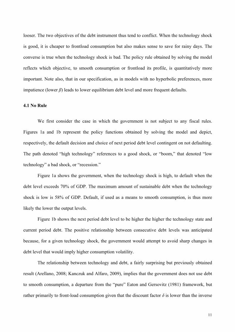
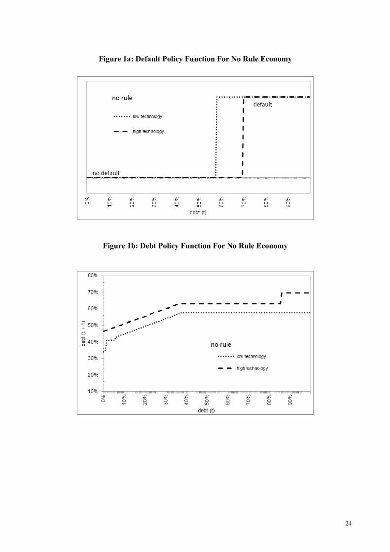
4.1 No Rule

We first consider the case in which the government is not subject to any fiscal rules.

Figures 1a and 1b represent the policy functions obtained by solving the model and depict,

respectively, the default decision and choice of next period debt level contingent on not defaulting.

The path denoted “high technology” references to a good shock, or “boom,” that denoted “low

technology” a bad shock, or “recession.”

Figure 1a shows the government, when the technology shock is high, to default when the

debt level exceeds 70% of GDP. The maximum amount of sustainable debt when the technology

shock is low is 58% of GDP. Default, if used as a means to smooth consumption, is thus more

likely the lower the output levels.

Figure 1b shows the next period debt level to be higher the higher the technology state and

current period debt. The positive relationship between consecutive debt levels was anticipated

because, for a given technology shock, the government would attempt to avoid sharp changes in

debt level that would imply higher consumption volatility.

The relationship between technology and debt, a fairly surprising but previously obtained

result (Arellano, 2008; Kanczuk and Alfaro, 2009), implies that the government does not use debt

to smooth consumption, a departure from the “pure” Eaton and Gersovitz (1981) framework, but

rather primarily to front-load consumption given that the discount factor δ is lower than the inverse

12

of the risk-free interest rate. Consumption smoothing is mostly achieved, as noted earlier, through

default, as in contingent debt service models such as that of Grossman and Van Huyck (1988).

Calculating the invariant distribution of the states, we determine the government to be

excluded from the market 3.2% of the time and average debt to be 60.1% of output, as reported in

the first line of Table 2. These results are broadly consistent with the stylized facts. Notice that by

assuming hyperbolic preferences on the part of the government, the model can reproduce the level

of debt and frequency of default typical of emerging markets, even if the household impatience

parameter is calibrated to interest rates.

4.2 Optimal Fiscal Rule

We next consider the case of the optimal fiscal rule. This benchmark corresponds to what

the Amador, Werning and Angeletos (2006) denominate the “first-best allocation”, and Halac and

Yared (2014) denominate “ex-ante optimal rule”. In our setup, this corresponds to the case of β =

1, if the rule was implemented last period, just after the government expenditure. Our analysis

contrasts with these papers in that there is no private information about the technology shocks. In

the latter, the optimal rule has to balance discretion with commitment, and is shown to be history

dependent, as it provides dynamic incentives. In our simpler case, given the absence of private

information, the first best policy can be implemented with full commitment, that is, by giving the

government a pre-determined contingent path of efficient consumption.

The invariant distribution properties of the economy under the optimal fiscal rule are

reported in the second row of Table 2. Under the optimal rule, the invariant distribution displays no

default and average debt level drops to 50.2% of GDP. In other words, the government present bias

is responsible for debt over-accumulation of about 10% of GDP and the occurrence of default

episodes.

13

Table 2 also compares, in terms of consumption, the welfare level of the economy under

the optimal rule and no rule. Considering, for both economies, the transition path from a starting

point with no debt to their respective invariant distribution, we obtain that adoption of the optimal

rule results in welfare gains of 0.277% of GDP, substantial compared to typical business cycle

welfare gains.

Figures 2a and 2b depict, respectively, the government’s default decision and choice of

next period debt level contingent on not defaulting. Figure 2a looks like Figure 1a, but has

different threshold axis values. As with no rule, default is more likely the lower the output levels.

The maximum amount of sustainable debt is 63% of GDP under a high, and 50% of GDP under a

low, technology shock. Although there is no default in equilibrium, the threshold values for default

are lower under the optimal than under no rule.

Comparing Figure 2b with Figure 1b reveals the optimal policy to also have similar

qualitative properties to the solution with no fiscal rule. Again, contrary to the usual intuition, debt

accumulation does not increase when the economy is hit by a bad shock. In other words, whereas

default is (potentially) used to smooth consumption, debt is used to tilt the consumption profile,

and this holds regardless of the fact that default does not occur in equilibrium, at least after the

economy has converged to its invariant distribution.

Figure 2b shows that when the debt level is relatively low, the economy saves the same

regardless of the output shock. When the debt level is high, however, the economy borrows more

in booms than in recessions because of the countercyclical interest rate schedules. In other words,

when debt (and the incentive to default) is greater, the borrower would like to borrow heavily

during bad shocks, but cannot because such financial contracts are too expensive. Consequently,

when debt is large the optimal fiscal policy is pro-cyclical.

14

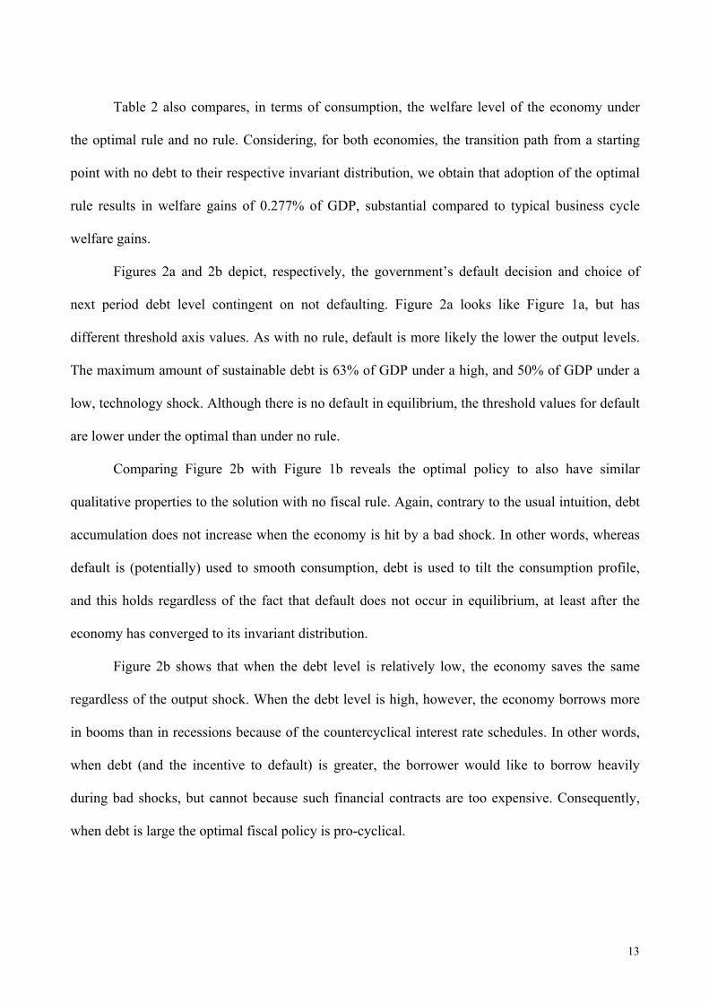
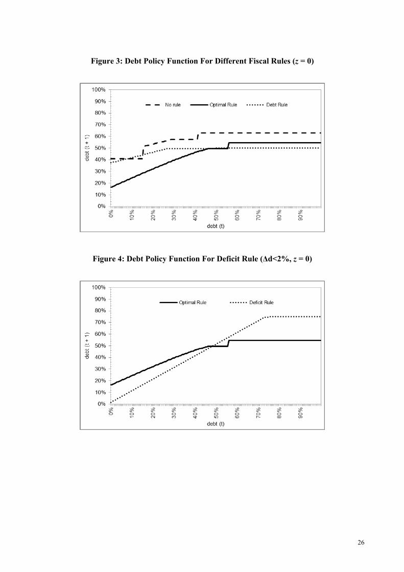
4.3 Debt Rules

We now consider the case of simple debt rules under the hypothesis that the government is

present biased (β = 0.70). These rules prohibit the government from choosing debt levels above a

previously set threshold. We solve for many thresholds and report the corresponding invariant

distribution properties in Table 2.

Note that when the debt threshold is set to 65% or 60% of GDP, the average debt level is

lower than under the no rule case but smaller than the threshold. Thus, the threshold is constraining

debt accumulation, but the government still has some margin. Additionally, for these threshold

levels the frequency of default is as high as under no rule.

When the debt threshold is set to 55% of GDP or lower, the invariant distribution debt level

is exactly equal to the threshold. Debt accumulation becomes, in fact, binding all the time and there

is no longer default in equilibrium (after converging to the invariant distribution).

Figure 3 depicts, for the case in which output is neither high nor low (i.e., z = 0), the policy

function for the cases with no rule, with the optimal fiscal rule, and with a simple rule with

threshold d ≤ 50% of GDP. Note that the simple rule implies an average debt level similar to the

optimal rule, but the constraint affects consumption smoothing, making the government

accumulate the same level of debt regardless of its previous indebtedness.

Welfare gains vary widely depending on debt threshold. When the threshold is too high or

too low, the simple rules, incur substantial welfare losses even relative to no rule. In the case of

very high threshold levels, the rule does not prevent default but limits consumption smoothing.

When the threshold levels are too low, the costs of preventing the sovereign to front-load

consumption outweigh any gain from preventing defaults. More interesting, when the threshold is

set to 50%, welfare gain is virtually equal to that of the optimal rule. That is, a very simple rule can

yield gains comparable to a fairly complex one.

15

We believe this finding may have relevant policy implications. Threshold debt rules, being

easily contractible and yielding welfare gains virtually equal to those afforded by the optimal fiscal

rule, would seem to be the better alternative for implementation in practice.

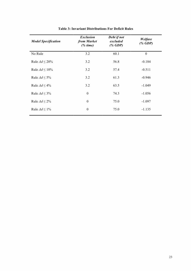
4.4 Deficit Rules

Lastly, we consider the case of simple deficit rules, again under the hypothesis that the

government is present biased (β = 0.70). These rules prohibit the government from choosing deficit

levels (or changes in debt, Δd ≡ dt+1 – dt) above a previously set threshold. We solve for many

thresholds and report the corresponding invariant distribution properties in Table 3.

Note that as the maximum amount of deficit is reduced, and the constraint becomes

binding, we observe fewer defaults and higher amounts of debt. It is unexpected, but promising,

that the deficit constraint can generate high amounts of debt, and thus more frontloading, without

incurring the costs of default. But examination of the welfare implications shows the arrangement

to not be working as expected.

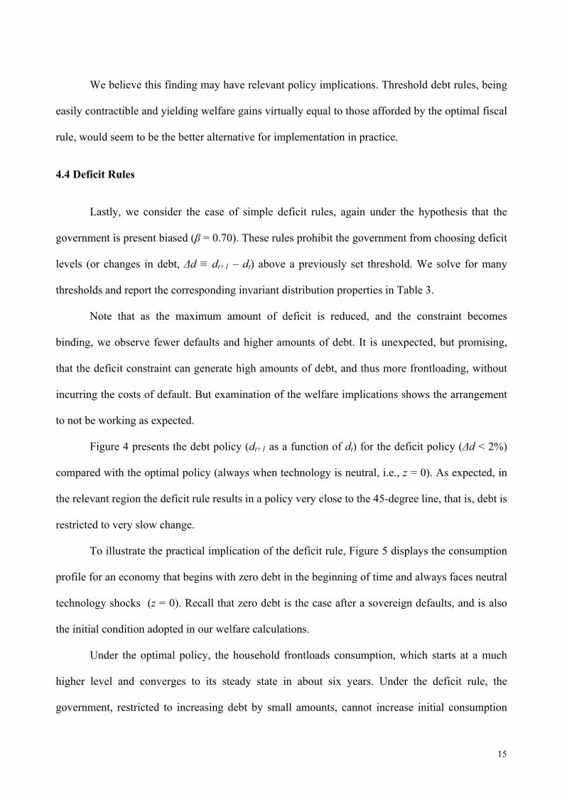
Figure 4 presents the debt policy (dt+1 as a function of dt) for the deficit policy (Δd < 2%)

compared with the optimal policy (always when technology is neutral, i.e., z = 0). As expected, in

the relevant region the deficit rule results in a policy very close to the 45-degree line, that is, debt is

restricted to very slow change.

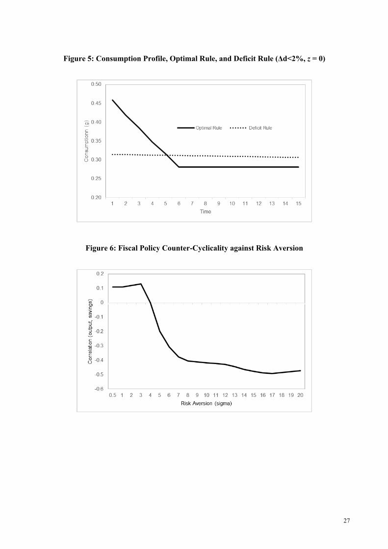
To illustrate the practical implication of the deficit rule, Figure 5 displays the consumption

profile for an economy that begins with zero debt in the beginning of time and always faces neutral

technology shocks (z = 0). Recall that zero debt is the case after a sovereign defaults, and is also

the initial condition adopted in our welfare calculations.

Under the optimal policy, the household frontloads consumption, which starts at a much

higher level and converges to its steady state in about six years. Under the deficit rule, the

government, restricted to increasing debt by small amounts, cannot increase initial consumption

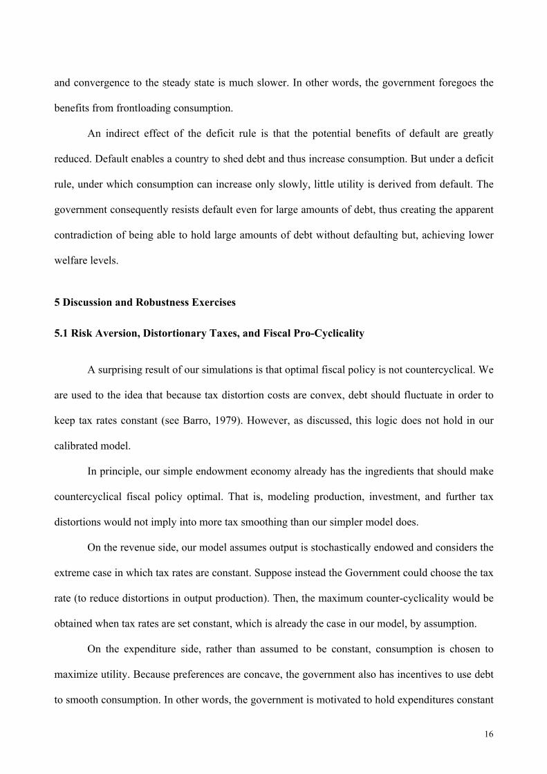
16

and convergence to the steady state is much slower. In other words, the government foregoes the

benefits from frontloading consumption.

An indirect effect of the deficit rule is that the potential benefits of default are greatly

reduced. Default enables a country to shed debt and thus increase consumption. But under a deficit

rule, under which consumption can increase only slowly, little utility is derived from default. The

government consequently resists default even for large amounts of debt, thus creating the apparent

contradiction of being able to hold large amounts of debt without defaulting but, achieving lower

welfare levels.

5 Discussion and Robustness Exercises

5.1 Risk Aversion, Distortionary Taxes, and Fiscal Pro-Cyclicality

A surprising result of our simulations is that optimal fiscal policy is not countercyclical. We

are used to the idea that because tax distortion costs are convex, debt should fluctuate in order to

keep tax rates constant (see Barro, 1979). However, as discussed, this logic does not hold in our

calibrated model.

In principle, our simple endowment economy already has the ingredients that should make

countercyclical fiscal policy optimal. That is, modeling production, investment, and further tax

distortions would not imply into more tax smoothing than our simpler model does.

On the revenue side, our model assumes output is stochastically endowed and considers the

extreme case in which tax rates are constant. Suppose instead the Government could choose the tax

rate (to reduce distortions in output production). Then, the maximum counter-cyclicality would be

obtained when tax rates are set constant, which is already the case in our model, by assumption.

On the expenditure side, rather than assumed to be constant, consumption is chosen to

maximize utility. Because preferences are concave, the government also has incentives to use debt

to smooth consumption. In other words, the government is motivated to hold expenditures constant

17

and thus implement a countercyclical fiscal policy. Our calibrated results indicate, however, that

this motive is dominated by other motivations, in particular, under the optimal fiscal rule, to use

debt to frontload rather than smooth consumption.

To investigate how quantitatively robust this result is we modify the model to increase the

gains from consumption smoothing. A simple way to do so is to modify the calibration by

increasing the risk aversion parameter σ. Because this parameter also plays the role of inter-

temporal elasticity, it controls the benefits of smoothing consumption.

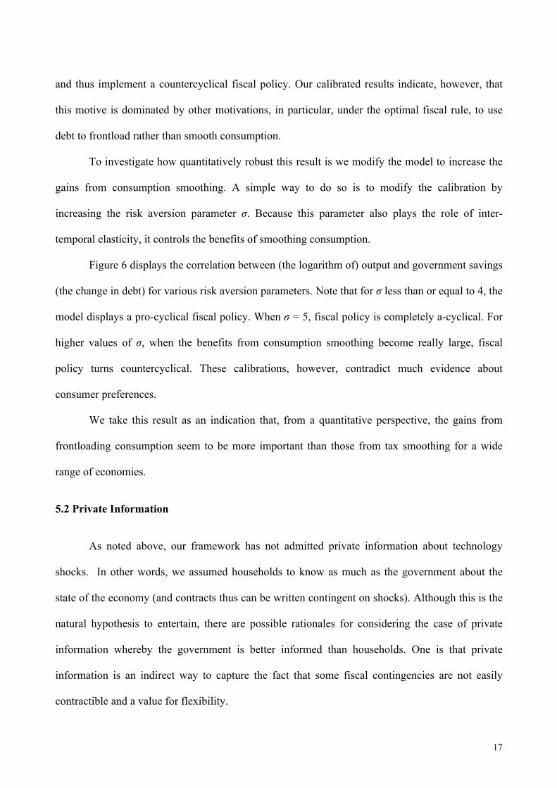
Figure 6 displays the correlation between (the logarithm of) output and government savings

(the change in debt) for various risk aversion parameters. Note that for σ less than or equal to 4, the

model displays a pro-cyclical fiscal policy. When σ = 5, fiscal policy is completely a-cyclical. For

higher values of σ, when the benefits from consumption smoothing become really large, fiscal

policy turns countercyclical. These calibrations, however, contradict much evidence about

consumer preferences.

We take this result as an indication that, from a quantitative perspective, the gains from

frontloading consumption seem to be more important than those from tax smoothing for a wide

range of economies.

5.2 Private Information

As noted above, our framework has not admitted private information about technology

shocks. In other words, we assumed households to know as much as the government about the

state of the economy (and contracts thus can be written contingent on shocks). Although this is the

natural hypothesis to entertain, there are possible rationales for considering the case of private

information whereby the government is better informed than households. One is that private

information is an indirect way to capture the fact that some fiscal contingencies are not easily

contractible and a value for flexibility.

18

How would our results change if only the government observed the technology shock? The

optimal policy would be much more complex, as shown by Halac and Yared (2014), but would

yield welfare gains (to households) less than or equal to those obtained under the optimal rule with

complete information. More precisely, the welfare gains of the private information optimal rule lie

somewhere between the welfare gains under the public information optimal rule and simple debt

threshold rules.

That welfare gains under the simple debt rule are almost identical to those under the

optimal rule, as highlighted in our analysis, is a good reason for using the simple threshold rule,

given that it is easily contractible. One can conclude that the same policy implication holds when

there is private information.

5.3 Self-Interested (Non-Benevolent) Government

The analysis in the previous sections hypothesized a benevolent government with quasi-

hyperbolic preferences that motivated adoption of fiscal rules. A vast literature in political

economy analyses over accumulation of debt by non-benevolent, or self-interested, governments.

A simple way to capture this possibility in our framework is to set β = 1 and calibrate δgov

such that our artificial economy displays observed debt levels consistent. That is, by supposing that

government preferences are not time inconsistent, but differ from those of the country’s citizens,

who are less impatient.

Setting δgov = 0.80, the invariant distribution displays debt equal to 62% of GDP and

projects default to occur 3.2% of the time, which figures are broadly consistent with both the

stylized facts and our basic calibration. As expected, the policy functions are also quite similar.

If the government discount factor is δgov = 0.80 and the citizens’ discount factor δ = 0.90,

the same policy implications as before would apply. The optimal rule and results of simple

threshold rules would also be the same as before.

19

An important omission from the analysis is why the optimal rule (or threshold rules) would

be applied. The self-interested government would certainly oppose adoption of such rules.

Although we do not analyze how, citizens need somehow, as by means of elections, to discipline

politicians and force them to adopt the rules.

6 Conclusion

Emerging countries, as they catch up to developed ones, can borrow in order to frontload

their consumption profile. In practice, however, they tend to over borrow and often resort to

defaulting on their debt. Governments’ preferences, for reasons of political economy or

aggregation of heterogeneous citizens’ preferences, may display a present bias.

Fiscal rules are a potentially useful commitment technology to solve this problem. In the

context of a traditional model of sovereign debt and default, we analyze the welfare gains from

alternative fiscal rules. We find the gains from the optimal fiscal rule to be economically relevant,

and observe that the optimal fiscal rule does not entail pro-cyclical fiscal policy. Additionally, a

simple, easily contractible threshold rule can generate gains virtually as high as the optimal rule.

7 References

Aguiar, M. and M. Amador. 2014. “Sovereign Debt.” In Handbook of International Economics

Vol 4, eds. G. Gopinath, E. Helpman and K. Rogoff. North-Holland: 647-87.

Aguiar, M. and M. Amador. 2011. “Growth Under the Shadow of Expropriation,” Quarterly

Journal of Economics 126: 651–697.

Aguiar, M. and G. Gopinath. 2006. “Defaultable Debt, Interest Rates and the Current Account,”

Journal of International Economics 69: 64-83.

Alesina, A. and A. Drazen. 1991. “Why Are Stabilizations Delayed?” American Economic Review

81(5): 1170-1188.

20

Alesina, A. and A. Passalacqua. 2015. “The Political Economy of Government Debt” manuscript

in preparation for the Handbook of Macroeconomics edited by John Taylor and Harald

Uhlig.

Alesina, A. and G. Tabelini. 2008. “Why Is Fiscal Policy Often Pro-cyclical?” Journal of the

European Economic Association 6(5): 1006-36.

Alfaro, L, and F. Kanczuk. 2005 “Sovereign Debt As a Contingent Claim: A Quantitative

Approach.” Journal of International Economics 65(2): 297-214.

Alfaro, L. and F. Kanczuk. 2009. “Optimal Reserve Management and Sovereign Debt,” Journal of

International Economics 77(1): 23-36.

Amador, M., I. Werning and G.-MS Angeletos. 2006. “Commitment vs. Flexibility,”

Econometrica 74, 365-96.

Angeletos, G.-MS, D. Laibson, J. Tobacman, A. Repetto and S. Weinberg. 2001. “The Hyperbolic

Consumption Model: Calibration, Simulation, and Empirical Evaluation,” Journal of

Economic Perspectives 15(3): 47-68.

Arellano, C. 2008. “Default Risk and Income Fluctuations in Emerging Markets,” American

Economic Review 98(3): 690-712.

Bauducco S. and F. Caprioli. 2014. “Optimal Fiscal Policy in a Small Open Economy with Limited

Commitment,” Journal of International Economics 93(2): 302-15.

Barro, R. J. 1979. “On the Determination of the Public Debt,” The Journal of Political Economy,

87(5): 940-97.

Eaton, J. and M. Gersovitz. 1981. “Debt with Potential Repudiation: Theoretical and Empirical

Analysis,” The Review of Economic Studies 48: 289-309.

Grossman, H. I. and J. B. Van Huyck. 1988. “Sovereign Debt as a Contingent Claim: Excusable

Default, Repudiation, and Reputation,” American Economic Review 78:1088-97.

21

Halac, M. and P. Yared. 2014. “Fiscal Rules and Discretion under Persistent Shocks,”

Econometrica 82(5): 1557-1614.

Halac, M. and P. Yared. 2015. “Fiscal Rules and Discretion in a World Economy,” Working

Paper.

Hatchondo, J. C., L. Martinez and F. Roch. 2015 “Fiscal Rules and the Sovereign Default

Premium,” Working Paper.

Jackson, M. O. and L. Yariv. 2014. “Present Bias and Collective Choice in the Lab,” American

Economic Review 104: 4184-4204.

Jackson, M. O. and L. Yariv 2015. “Collective Dynamic Choice: The Necessity of Time

Inconsistency,” American Economic Journal: Microeconomics 7(4): 150-78.

Kaminsky, G., C. Reinhart and C. Vegh. 2005. “When It Rains It Pours: Pro-cyclical Macro-

policies and Capital Flows.” In NBER Macroeconomics Annual 2004, eds. M. Gutler and

K. S. Rogoff. MIT Press: 11-53.

Mendoza, E. and V. Yue. “A General Equilibrium Model of Sovereign Default and Business

Cycles,” The Quarterly Journal of Economics 127, 889-946.

Laibson, D. 1997. “Golden Eggs and Hyperbolic Discounting,” Quarterly Journal of Economics,

112: 443-78.

Persson, T. and L.E.O. Svensson. 1989. “Why a Stubborn Conservative would Run a Deficit:

Policy with Time-Inconsistent Preferences,” Quarterly Journal of Economics 104: 325-45.

Reinhart, C. and K. Rogoff. 2009. This Time is Different: Eight Centuries of Financial Follies.

Princeton, New Jersey: Princeton University Press.

Schmidt-Hebbel, K. and R. Soto. 2016. “Fiscal Rules in the World,” Working Paper.

Vegh, C. and G. Vuletin. 2012. “How Is Tax Policy Conducted over the Business Cycle?”

American Economic Journal: Economic Policy 7: 327-70.

22

Table 1: Calibration

Technology autocorrelation α = 0.85

Technology standard deviation σ = 0.044

Probability of redemption θ = 0.20

Output costs ϕ = 0.10

Risk aversion σ = 2

Risk free interest rate ρ = 0.04

Tax rate τ = 0.30

Discount factor δ = 0.90

Hyperbolic discount factor β = 0.70

Table 2: Invariant Distributions For Alternative Fiscal Rules

Model Specification Exclusion

from Market (% time)

Debt if not excluded (% GDP)

Welfare (% GDP)

No Rule 3.2 60.1 0

Optimal Rule 0 50.2 0.277

Rule d ≤ 65% 3.2 59.8 -0.214

Rule d ≤ 60% 3.2 57.8 -0.163

Rule d ≤ 55% 0 55.0 0.259

Rule d ≤ 50% 0 50.0 0.276

Rule d ≤ 45% 0 45.0 0.275

Rule d ≤ 40% 0 40.0 0.212

Rule d ≤ 35% 0 35.0 0.129

Rule d ≤ 30% 0 30.0 0.024

Rule d ≤ 20% 0 20.0 -0.257

Rule d ≤ 10% 0 10.0 -0.656

Rule d ≤0 0 0 -1.141

23

Table 3: Invariant Distributions For Deficit Rules

Model Specification Exclusion

from Market (% time)

Debt if not excluded (% GDP)

Welfare (% GDP)

No Rule 3.2 60.1 0

Rule Δd ≤ 20% 3.2 56.8 -0.184

Rule Δd ≤ 10% 3.2 57.4 -0.511

Rule Δd ≤ 5% 3.2 61.3 -0.946

Rule Δd ≤ 4% 3.2 63.5 -1.049

Rule Δd ≤ 3% 0 74.3 -1.056

Rule Δd ≤ 2% 0 75.0 -1.097

Rule Δd ≤ 1% 0 75.0 -1.135

24

Figure 1a: Default Policy Function For No Rule Economy

Figure 1b: Debt Policy Function For No Rule Economy

25

Figure 2a: Default Policy Function For Optimal Rule

Figure 2b: Debt Policy Function For Optimal Rule

26

Figure 3: Debt Policy Function For Different Fiscal Rules (z = 0)

Figure 4: Debt Policy Function For Deficit Rule (Δd<2%, z = 0)

27

Figure 5: Consumption Profile, Optimal Rule, and Deficit Rule (Δd<2%, z = 0)

Figure 6: Fiscal Policy Counter-Cyclicality against Risk Aversion