level, slope, curvature of the sovereign yield curve, and fiscal
TRANSCRIPT

Work ing PaPer Ser i e Sno 1276 / DeCeMBer 2010
level, SloPe,
Curvature of
the Sovereign
yielD Curve,
anD fiSCal
Behaviour
by António Afonso and Manuel M.F. Martins
WORKING PAPER SER IESNO 1276 / DECEMBER 2010
In 2010 all ECB publications
feature a motif taken from the
€500 banknote.
LEVEL, SLOPE, CURVATURE OF
THE SOVEREIGN YIELD CURVE,
AND FISCAL BEHAVIOUR 1
by António Afonso 2 and Manuel M.F. Martins 3
1 We are grateful to Ad van Riet and to an anonymous referee for useful comments.
2 ISEG/TULisbon – Technical University of Lisbon, Department of Economics; UECE – Research Unit on Complexity and Economics,
R. Miguel Lupi 20, 1249-078 Lisbon, Portugal and European Central Bank, Directorate General Economics,
Kaiserstrasse 29, D-60311 Frankfurt am Main, Germany. UECE is supported by FCT (Fundação para a
Ciência e a Tecnologia, Portugal), financed by ERDF and Portuguese funds.
E-mails: [email protected] and [email protected]
3 University of Porto, Faculty of Economics, Cef.up – Centre for Economics and Finance at the University of Porto,
Rua Dr Roberto Frias, s/n 4200 464 Porto Portugal. Cef.up is supported by FCT (Fundação para a Ciência
e a Tecnologia, Portugal), financed by ERDF and Portuguese funds. E-mail: [email protected].
Manuel M.F. Martins thanks the Fiscal Policies Division of the ECB for its hospitality.
This paper can be downloaded without charge from http://www.ecb.europa.eu or from the Social Science Research Network electronic library at http://ssrn.com/abstract_id=1718344.
NOTE: This Working Paper should not be reported as representing the views of the European Central Bank (ECB). The views expressed are those of the authors
and do not necessarily reflect those of the ECB.

© European Central Bank, 2010
AddressKaiserstrasse 2960311 Frankfurt am Main, Germany
Postal addressPostfach 16 03 1960066 Frankfurt am Main, Germany
Telephone+49 69 1344 0
Internethttp://www.ecb.europa.eu
Fax+49 69 1344 6000
All rights reserved.
Any reproduction, publication and reprint in the form of a different publication, whether printed or produced electronically, in whole or in part, is permitted only with the explicit written authorisation of the ECB or the author(s).
Information on all of the papers published in the ECB Working Paper Series can be found on the ECB’s website, http://www.ecb.europa.eu/pub/scientific/wps/date/html/index.en.html
ISSN 1725-2806 (online)

3ECB
Working Paper Series No 1276December 2010
Abstract 4
Non-technical summary 5
1 Introduction 7
2 Literature overview 8
3 Methodology 14
3.1 The yield curve latent factors 15
3.2 Setting up the VAR 17
4 Empirical analysis 18
4.1 Data 18
4.2 Fitting the yield curve 19
4.3 VAR analysis 28
5 Conclusion 47
References 49
Appendix 54
Annexes 56
CONTENTS
4ECBWorking Paper Series No 1276December 2010
Abstract
We study fiscal behaviour and the sovereign yield curve in the U.S. and Germany in the period 1981:I-2009:IV. The latent factors, level, slope and curvature, obtained with the Kalman filter, are used in a VAR with macro and fiscal variables, controlling for financial stress conditions. In the U.S., fiscal shocks have generated (i) an immediate response of the short-end of the yield curve, associated with the monetary policy reaction, lasting between 6 and 8 quarters, and (ii) an immediate response of the long-end of the yield curve, lasting 3 years, with an implied elasticity of about 80% for the government debt ratio shock and about 48% for the budget balance shock. In Germany, fiscal shocks entail no significant reactions of the latent factors and no response of the monetary policy interest rate. In particular, while (i) budget balance shocks created no response from the yield curve shape, (ii) surprise increases in the debt ratio caused some increase in the short-end and the long-end of the yield curve in the following 2nd and 3rd
quarters.
Keywords: yield curve, fiscal policy, financial markets. JEL Classification Numbers: E43, E44, E62, G15, H60.
5ECB
Working Paper Series No 1276December 2010
Non-technical summary In this paper, we use the macro-finance analytical framework of Diebold,
Rudebusch and Aruoba (2006) and enrich their empirical model of the economy with
variables representing fiscal policy as well as variables related to financial factors,
meant to control for the financial stress conditions faced by the economy. Our set of
variables allows both for a reasonable identification of the main policy shocks, and also
for a study of the economy in the low-yield environment and the ensuing financial and
economic crisis of 2008-2009.
More specifically, the paper empirically studies the dynamic relation between fiscal
developments – government debt and the budget deficit – and the shape of the sovereign
yield curves for the U.S. and for Germany. The shape of the yield curve is measured by
maximum-likelihood estimates of the level, slope and curvature, obtained with the
Kalman filter, following the state-space specification of the Nelson and Siegel (1987)
model.
The yield curve latent factors and the fiscal variables are related in country-specific
VAR models that further comprise the variables typically considered in macro-finance
models – real output, inflation and the monetary policy interest rate – as well as a
variable meant to control for the financial conditions. We contribute to the literature by
specifying and estimating VAR models that are not ex-ante restricted in their lag length
and which account for the dynamic effects of fiscal policy on the whole shape of the
curve, rather than estimating the elasticity of a specific interest rate at a specific time-
horizon as is more often the case in analyses of the relation between fiscal behaviour
and sovereign yields.
The samples begin in the early 1980s and end in the last quarter of 2009, thus
including at least two recessions (1992-93, 2001), the recent economic and financial
crisis (2008-09), the Volcker chairmanship of the FED (1979-1987) in the U.S., and for
the case of Germany, the reunification, the approval of the Maastricht Treaty (1992),
and the creation of the euro (1999).
In the U.S., fiscal shocks have led to an immediate response of the short-end of the
yield curve that is apparently associated with the reaction of monetary policy to the
macroeconomic effects of fiscal developments. Such reaction lasts a year and a half (for
debt ratio shocks) and two years (for budget balance shocks). Fiscal shocks further led
to an immediate response of the long-end segment of the yield curve – with fiscal
expansions leading to an increase in long-term sovereign yields – that lasts three years.
At the height of the effects, our estimates imply an elasticity of long-term yields to a
debt ratio shock of about 0.80 (10th-11th quarters after the shock) and an elasticity to a
budget balance shock of about 0.48 (12 quarters after the shock). Our results differ from
the findings of papers that found a smaller elasticity of long yields to the debt ratio than
6ECBWorking Paper Series No 1276December 2010
to the budget balance, although such studies do not consider the full yield curve latent
factors as we do.
Moreover, shocks to the change in the debt ratio (comparable to a shock in the
budget balance) account for most of the variance of the errors in forecasting the level of
the yield curve at horizons above 1 year and explain 40% of such variance at a 12
quarter horizon. Such shocks also account for substantial, albeit smaller, fractions of the
variance of the error in forecasting the slope and the curvature of the yield curve.
Shocks to the budget balance ratio are also relevant in accounting for the variance of the
errors of the yield curve factors. Highlighting the importance of studying fiscal shocks
we could not reject the hypotheses that the change in the debt ratio causes, in the
Granger sense, the shape of the yield curve. As regards the budget balance, Granger
causality has only been found for the slope and the curvature.
The results for Germany differ markedly from those obtained for the U.S. On the
one hand, fiscal shocks entail no comparable reactions of the yield curve factors. On the
other hand, they generate no significant response of the monetary policy interest rate.
The results also differ across the two alternative fiscal variables. Shocks to the budget
balance ratio create no response from any component of the yield curve shape, while a
surprise increase in the change of the debt ratio causes a decline in the concavity of the
yield curve that implies an increase in both the short-end and the long-end of the yield
curve; yet, such reaction is very quick and transitory, as it is statistically significant only
during the 2nd and 3rd quarters after the shock. This can be seen as a response of capital
markets to growing sovereign indebtedness also in the case of Germany. Such result
seems due to the period before 1999, since, as the exploratory sub-sample analyses
suggest, for both types of fiscal shocks, the impact of fiscal behaviour on the yield curve
was mitigated after 1999. During 1981-1998, expansionary fiscal shocks have led to
increases in the yields of the shortest and the longest maturities during the subsequent
three quarters.
In Germany, fiscal shocks have been overall unimportant in accounting for the
variance of the errors in forecasting the yield curve latent factors, with two exceptions.
First, the debt ratio shocks explain a not negligible part of the errors in forecasting the
curvature – consistently with the impulse response analysis; second, budget balance
shocks are somewhat relevant in accounting for errors in forecasting the level of the
yield curve. In the case of Germany, the results from Granger causality tests agree with
the impulse responses and forecast errors variance decompositions, as it is not possible
to reject the hypothesis that either the debt ratio or the budget balance Granger-cause
any of the yield curve factors.
7ECB
Working Paper Series No 1276December 2010
1. Introduction
A relevant question, notably for policy makers, is to understand, as far as possible,
what are the relations between fiscal developments and the shape of the sovereign yield
curve, as well as the dynamic patterns of such relation. One can expect to observe both a
bi-directional relationship and similarities across the main developed countries.
In the related literature there are a number of papers trying to uncover the relation of
the main fiscal variables with the long-term end of the yield curve in specific time-
horizons, and a few studies assess such relation at some additional points of the curve,
namely its short-term end. Nevertheless, an attempt at thoroughly uncovering the
dynamic relations between fiscal policy developments and the whole shape of the yield
curve seems to be lacking. It is well known from the finance literature that this shape
may be parsimoniously represented by estimates of the level, slope and curvature of the
yield curve. Such an approach to the yield curve characterisation has been followed by a
recent macro-finance literature mainly focused on non-fiscal macro variables, namely
real output, inflation and the monetary policy rate.
In this paper, we use the macro-finance analytical framework and enrich the
empirical model of the economy with variables representing fiscal policy as well as
additional variables related to financial factors, meant to control for the financial stress
conditions faced by the economy. Our set of variables allows both for a reasonable
identification of the main policy shocks, and also for a study of the economy in the low-
yield environment and the ensuing financial and economic crisis of 2008-2009.
More specifically, the paper empirically studies the dynamic relation between fiscal
developments – government debt and the budget deficit – and the shape of the sovereign
yield curves for the U.S. and for Germany. The shape of the yield curve is measured by
estimates of the level, slope and curvature in the Nelson and Siegel (1987) tradition,
following the state-space specification and maximum-likelihood estimation with the
Kalman filter suggested by Diebold and Li (2006) and Diebold, Rudebusch and Aruoba
(2006).
The yield curve latent factors and the fiscal variables are related in country-specific
VAR macro-finance models that further comprise the variables typically considered in
macro-finance models – real output, inflation and the monetary policy interest rate – as
well as a variable meant to control for the financial conditions. The evidence is based on
impulse response function analysis, forecast error variance decomposition and Granger
causality tests. In this context, the novelty of our paper consists of the inclusion of fiscal

8ECBWorking Paper Series No 1276December 2010
variables and a control for financial conditions in an empirical model akin to the one of
Diebold, Rudebusch and Aruoba (2006). We contribute to the literature by specifying
and estimating VAR models that are not ex-ante restricted in their lag length and which
account for the dynamic effects of fiscal policy on the whole shape of the curve, rather
than estimating the elasticity of a specific interest rate at a specific time-horizon as is
more often the case in analyses of the relation between fiscal behaviour and sovereign
yields.
The samples begin in the early 1980s and end in the last quarter of 2009, thus
including at least two recessions (1992-93, 2001), the recent economic and financial
crisis (2008-09), the Volcker chairmanship of the FED (1979-1987) in the U.S., and for
the case of Germany, the reunification, the approval of the Maastricht Treaty (1992),
and the creation of the euro (1999).
Changes in policy regimes can be an issue for empirical work as they carry along
the possibility of structural breaks in the VAR. We check whether the issue is relevant
in the case of Germany, at the onset of the Economic and Monetary Union, however,
not enough data area available for the pre-reunification period to check for a possible
break due to the reunification.
As regards the US, changes in the fiscal regime are less clear than in the monetary
policy regime. Nevertheless, almost all sample period corresponds to the Greenspan
chairmanship of the FED and there is not enough data to test for a significant break
during the Volker chairmanship. We have checked whether starting the sample at 1986
rather than in 1981changed qualitatively the results and found that it does not.
The paper is organised as follows. Section two gives an overview of the literature.
Section three explains the methodology to obtain the yield curve latent factors and the
VAR specifications. Section four conducts the empirical analysis reporting the estimates
of the level, slope and curvature, as well as the VAR results. Finally, section five
concludes.
2. Literature overview
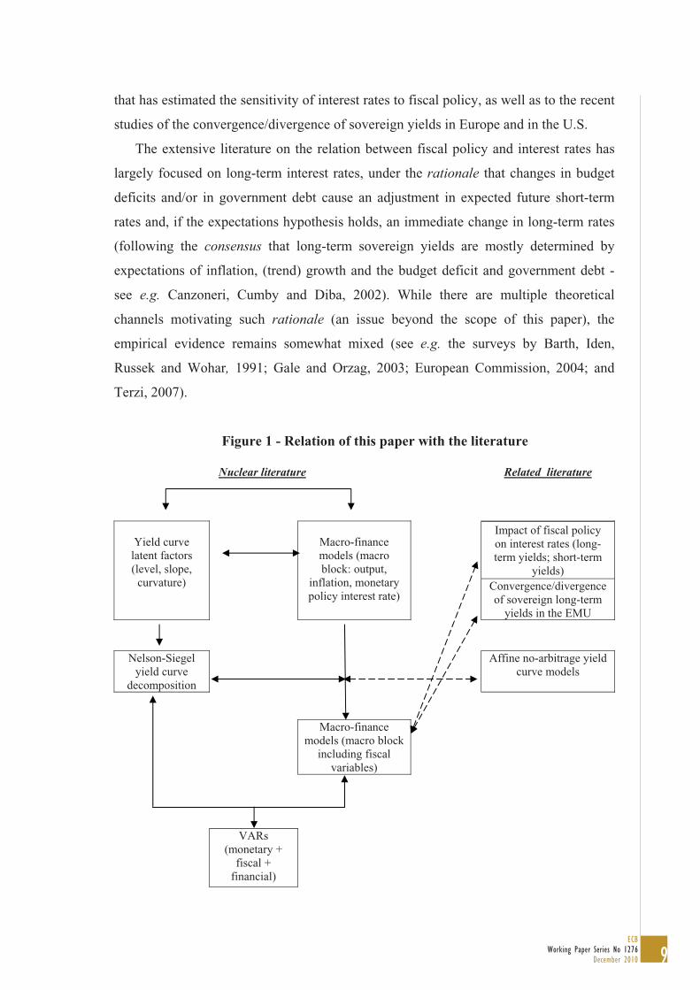
Figure 1 shows the strands of literature that connect with this paper, distinguishing
between nuclear and related literature. On the one hand, our study relates more closely
with the analyses that describe the shape of the yield curve estimating three latent
factors – level, slope and curvature – and then use these variables in VAR-based macro-
finance models of the economy. On the other hand, the paper adds to the large literature
9ECB
Working Paper Series No 1276December 2010
that has estimated the sensitivity of interest rates to fiscal policy, as well as to the recent
studies of the convergence/divergence of sovereign yields in Europe and in the U.S.
The extensive literature on the relation between fiscal policy and interest rates has
largely focused on long-term interest rates, under the rationale that changes in budget
deficits and/or in government debt cause an adjustment in expected future short-term
rates and, if the expectations hypothesis holds, an immediate change in long-term rates
(following the consensus that long-term sovereign yields are mostly determined by
expectations of inflation, (trend) growth and the budget deficit and government debt -
see e.g. Canzoneri, Cumby and Diba, 2002). While there are multiple theoretical
channels motivating such rationale (an issue beyond the scope of this paper), the
empirical evidence remains somewhat mixed (see e.g. the surveys by Barth, Iden,
Russek and Wohar, 1991; Gale and Orzag, 2003; European Commission, 2004; and
Terzi, 2007).
Figure 1 - Relation of this paper with the literature
Nuclear literature Related literature
Yield curve latent factors (level, slope,
curvature)
Macro-finance models (macro block: output,
inflation, monetary policy interest rate)
Impact of fiscal policy on interest rates (long-term yields; short-term
yields) Convergence/divergence of sovereign long-term
yields in the EMU
Nelson-Siegel yield curve
decomposition
Affine no-arbitrage yield curve models
Macro-finance
models (macro block including fiscal
variables)
VARs (monetary +
fiscal + financial)

10ECBWorking Paper Series No 1276December 2010
Overall, the literature warrants the following main conclusions. First, there seems to
be a significant impact of budget deficits and government debt on long-term interest
rates, especially detected in studies that use budget deficits and debt projections, rather
than current fiscal data (see e.g. Canzoneri, Cumby and Diba, 2002; Gale and Orzag,
2004; Laubach, 2009; Afonso, 2009; Hauner and Kumar, 2009). For instance,
Schuknecht, von Hagen and Wolswijk (2010) report that the interest rate effects of
budget deficits and government debt were significantly higher after the Lehmann
default.
Second, the sensitivity of interest rates to fiscal variables seems to be smaller in
Europe than in the US (see e.g. Codogno, Favero and Missale, 2003; Bernoth, von
Hagen and Schuknecht, 2006; Faini, 2006; Paesani, Strauch and Kremer, 2006; and, for
event studies, Afonso and Strauch, 2007; and Ardagna, 2009). Third, the relation differs
across different initial levels of government debt ratios (see e.g. Faini, 2006; Ardagna,
2009; Ardagna, Caselli and Lane, 2007). Fourth, the elasticity of interest rates to
government debt seems to be significantly smaller than the elasticity to the budget
deficit (see e.g. Laubach, 2009; Engen and Hubbard, 2004; Kinoshita, 2006; Chalk and
Tanzi, 2002).
A recent subset of this literature has studied the convergence (divergence) of
government bond yields in Europe, especially among the Euro Area countries’,
following the creation of the EMU and/or the recent financial crisis, with a large part of
the papers attributing a possible role to fiscal factors in such convergence (divergence).
These studies have also typically looked at long-term yields, especially 10-year
government bonds (see e.g. Attinasi, Checherita and Nickel, 2009; Haugh, Ollivaud and
Turner, 2009; Sgherri and Zoli, 2009; Manganelli and Wolswijk, 2009; Barrios, Iversen,
Lewandowska and Setzer, 2009, and Afonso and Rault, 2010), even when focusing on
the relevance of fiscal events (see e.g. Codogno, Favero, and Missale, 2003; and Afonso
and Strauch, 2007). In some cases, the empirical analysis has combined data from
sovereign debt issued at several maturities (Schuknecht, von Hagen and Wolswijk,
2010). Yet another part of this research has focused on the determinants – including the
fiscal ones – of the long-term yield spreads between new European Union countries and
other European states and benchmarks such as the US or the German bonds (see e.g.
Nickel, Rother and Rülke, 2009; Alexopolou, Bunda and Ferrando, 2009).
While most of the literature relating fiscal developments with interest rates has
looked at the long end part of the yield curve, some papers did analyse other segments
11ECB
Working Paper Series No 1276December 2010
of the curve. An early example is Elmendorf and Reifschneider (2002), who have
compared the effect of several fiscal policy actions on the 10-year treasury yield and the
monetary policy rate (Fed Funds rate), in order to disentangle the financial feed-backs
from fiscal policy. Another example is Canzoneri, Cumby and Diba (2002), who have
studied the effect of projections of cumulative budget deficits on the spread between 5-
year (or 10-year) and 3-month Treasury yields. More recently, Geyer, Kossmeier and
Pichler (2004) considered the spreads, relative to the German Bunds, of the yields of
two and nine years government bonds of Austria, Belgium, Italy and Spain, which they
related to a number of macro, fiscal and financial variables.
In addition, Ehrmann, Fratzscher, Gurkaynak and Swanson (forthcoming), used
daily yields of maturities between two and ten years to study the convergence of the
shape of the yield curves of Italy and Spain with those of France and Germany after the
EMU, looking at the first (level) and second (slope) principal components of the yield
curve. However, they have not considered the very short-end maturities and did not
explicitly relate the behaviour of the yield curves to fiscal variables.
Given our purpose of studying the dynamic relation between fiscal policy and the
shape of the sovereign yield curves, another nuclear strand of literature has developed
theoretical and empirical macro-finance models that explicitly consider the contour of
the whole yield curve and model their dynamic interactions with macroeconomic
variables. An important part of such literature has drawn on the Nelson and Siegel
(1987) decomposition of the yield curve into three latent factors that together allow for a
description of the yield curve shape at each moment.
Litterman and Scheinkman (1991) and Diebold and Li (2006) have interpreted the
above mentioned latent factors as Level, Slope and Curvature, and the latter suggested a
two-step procedure to estimate the factors recursively and iteratively. First, estimating
the three factors by non-linear-least squares (conditional on some a-priori regarding the
loadings of the slope and curvature at each maturity); second, using the estimates of the
factors for forecasting the yield curve. Diebold, Rudebusch and Aruoba (2006) argued
that such two-steps procedure is sub-optimal and suggested a one-step procedure based
on a state-space representation of the Nelson-Siegel model and its estimation by
maximum likelihood with the Kalman filter, which allows for estimating all the hyper-
parameters along with the time-varying parameters, i.e. the curve latent factors.
So far, most of the analyses within this approach have focused on the relation
between the yield-curve latent factors and monetary policy, inflation and real activity
12ECBWorking Paper Series No 1276December 2010
(see for example Diebold, Rudebusch and Aruoba, 2006; Carriero, Favero and
Kaminska, 2006; Dewachter and Lyrio, 2006; Hordahl, Tristani and Vestin, 2006;
Rudebusch and Wu, 2008; Hoffmaister, Roldós and Tuladhar, 2010). This may be
explained by the fact that such approach relates closely with the vast literature on the
power of the yield curve Slope (and possibly the Curvature) to predict fluctuations in
real economic activity and inflation – with the transmission mechanism largely seen as
involving monetary policy – as well as on the relation of the Level with inflation
expectations (see, for example, Ang, Piazzesi and Wei, 2006; Rudebusch and Williams,
2008 and the references therein).
While several studies such as Diebold, Rudebusch and Aruoba (2006) and Carriero,
Favero and Kaminska (2006) have used the Nelson-Siegel decomposition of the yield
curve, a sub-class of the macro-finance literature has used affine arbitrage-free models
of the yield curve. These models essentially enhance the Nelson-Siegel parsimonious
approach with no-arbitrage restrictions (see e.g. Ang and Piazzesi, 2003; Diebold,
Piazzesi and Rudebusch, 2005; Christensen, Diebold and Rudebusch, 2009;
Rudebusch, 2010, and the references therein). In this paper, we follow the Nelson-
Siegel method to decompose the yield curve into latent factors, and focus on enhancing
the empirical macro-finance model with fiscal policy variables.
Macro-finance analyses assessing the role of fiscal variables in the behaviour of the
whole yield curve do not abound, but there are some papers in that vein, which thus
relate closely to our paper. An early example is Dai and Philippon (2006), who have
developed an empirical macro-finance model for the U.S. including, in the macro block,
the monetary policy interest rate, inflation, real activity and the government budget
deficit. Their model combines a no-arbitrage affine yield curve comprising a fairly large
spectrum of maturities, with a set of structural restrictions that allow for identifying
fiscal policy shocks and their effects on the prices of bonds of different maturities. The
estimation of their over-identified no-arbitrage structural VAR allows them to conclude
that government budget deficits affect long-term interest rates, albeit temporarily (with
high long rates not necessarily turning into high future short-term rates). They estimate
that a one percentage point increase in the deficit ratio increases the 10-year rate by 35
basis points after three years, with fiscal policy shocks accounting for up to 13 percent
of the variance of forecast errors in bond yields. While focusing only on the US case
and using rather intricate identifying restrictions, their result that fiscal shocks
temporarily increase the yield curve slope merits attention, namely when assessing
13ECB
Working Paper Series No 1276December 2010
whether such result holds for Germany and whether it holds after controlling for the
financial factors that have been important in the recent crisis.
Another example is Bikbov and Chernov (2006), who have set-up a no-arbitrage
affine macro-finance model of the yield curve, inflation, real activity and two latent
factors. By means of a projection of the latent factors onto the macro variables, they
extract the additional information therein and interpret the projection residuals as
monetary and fiscal shocks, in view of their correlation with a measure of liquidity and
a measure of government debt growth. They find that real activity and inflation explain
almost all (80 percent) of the variation in the short-term interest rate, while the
exogenous monetary and fiscal shocks have a prominent impact on the short and long
end of the yield curve, respectively. Moreover, they find that jointly, they are as
important as inflation and real activity in explaining the long part of the term structure
and explain 50 percent of the slope variation. In particular, the slope is highly correlated
with the growth in public debt, a result that they find consistent with the anecdotal
evidence concerning the Clinton restrictive budget package on February 1993 as well as
with the November 1999 increase in taxes, during which the yield curve slope decreased
between 1.5 and 2 percentage points, due to the fall in long-term yields and no change
in the short-term yields.
Finally, a paper that is closer to ours – as it uses the Nelson-Siegel decomposition of
the yield curve, rather than a no-arbitrage model, and focuses on the effects of fiscal
policy on the yield curve – is Favero and Giglio (2006). They studied the effects of
fiscal policy on the spreads between the Italian government bond yields and the
Germany yields, under a pre and a post-EMU regime of expectations about fiscal policy
and looking at the whole yield curve rather than a range of maturities. Using quarterly
data for 1991:II-2006:I, they estimated the yield curve Level, Slope and Curvature and
then studied the relation between the debt-to-GDP ratio and the Level – interpreted as
the long-run component of the curve – as well as the Curvature – the medium-run
component – in a framework of Markov-switching regimes of expectations about fiscal
policy. Their estimates capture the change, with the EMU, from a higher public finances
expected risk to a lower risk expectations regime, with the estimated impact of the fiscal
variables on the yield curve depending on the expectations regime. Under unfavourable
fiscal expectations, they estimate that for every 10 percentage points of increase in the
Italian debt-to-GDP ratio the yield curve level tends to increase by 0.43 percentage

14ECBWorking Paper Series No 1276December 2010
points; and that such increase in the debt-to-GDP ratio would imply on average an
increase of 0.25 percentage points in the medium-term part of the yield curve.
3. Methodology
We contribute to the macro-finance literature at an applied level studying the
relation between the shape of the sovereign yield curve and fiscal behaviour in a
framework that is a development of the Rudebusch, Diebold and Aruoba’s (2006)
approach. In addition to including a fiscal variable and a control for financial
conditions, we estimate the VAR subsequently to the estimation of the yield curve
factors (in the spirit of Diebold and Li, 2006), which avoids restricting its lag length.
Our choice of the sample period and control variables allows us to take into account the
impact of the creation of the euro area, the recent global low-yield period and the 2008-
2009 financial crisis, as well as potential regime shifts such as the Volcker
chairmanship of the FED (1979-1987) in the U.S., and in the case of Germany the
reunification, the approval of the Maastricht Treaty (1992), and the creation of the euro
(1999).Regarding the computation of the yield curve three main latent factors – Level,
Slope and Curvature – we follow the parsimonious Nelson-Siegel approach to the
modelling of the yield curve used by e.g. Diebold and Li (2006) and Diebold,
Rudebusch and Aruoba (2006). Our choice for not following an arbitrage-free approach
is motivated by the arguments set out by Diebold and Li (2006, pp. 361-362) and
Diebold, Rudebusch and Aruoba (2006, pp. 333), stating that it is not clear that
arbitrage-free models are necessary or even desirable for macro-finance exercises.
Indeed, if the data abides by the no-arbitrage assumption, then the parsimonious but
flexible Nelson-Siegel curve should at least approximately capture it, and, if this is not
the case, then imposing it would depress the model’s ability to forecast the yield curve
and the macro variables.
Our methodological framework consists of two steps, run separately for each
country. In a first step, the three yield curve latent factors are estimated by maximum
likelihood using the Kalman filter, as in Diebold, Rudebusch and Aruoba (2006). In the
second step, we estimate country-specific VARs with the latent yield curve factors, the
traditional macroeconomic variables – output, inflation and the overnight interest rate –
a financial control variable – a financial stress index (FSI) – and a fiscal variable – the
budget balance ratio or the change in the debt-to-GDP ratio. Then, the analyses of the

15ECB
Working Paper Series No 1276December 2010
VAR dynamics, in particular of innovations to the fiscal variable, allow us to address
the question that motivates the paper.
3.1. The yield curve latent factors
We model the yield curve using a variation of the three-component exponential
approximation to the cross-section of yields at any moment in time proposed by Nelson
and Siegel (1987),
1 2 3
1 1( )
e ey e , (1)
where ( )y denotes the set of (zero-coupon) yields and is the corresponding maturity.
Following Diebold and Li (2006) and Diebold, Rudebusch and Aruoba (2006), the
Nelson-Siegel representation is interpreted as a dynamic latent factor model where 1 ,
2 and 3 are time-varying parameters that capture the level (L), slope (S) and
curvature (C) of the yield curve at each period t, while the terms that multiply the
factors are the respective factor loadings:
1 1( )t t t t
e ey L S C e . (2)
Clearly, tL may be interpreted as the overall level of the yield curve, as its loading
is equal for all maturities. The factor tS has a maximum loading (equal to 1) at the
shortest maturity which then monotonically decays through zero as maturities increase,
while the factor tC has a loading that is null at the shortest maturity, increases until an
intermediate maturity and then falls back to zero as maturities increase. Hence, tS and
tC may be interpreted as the short-end and medium-term latent components of the yield
curve, with the coefficient ruling the rate of decay of the loading of the short-term
factor and the maturity where the medium-term one has maximum loading.1
As in Diebold, Rudebusch and Aruoba (2006) we assume that tL , tS and tC follow
a vector autoregressive process of first order, which allows for casting the yield curve
latent factor model in state-space form and then using the Kalman filter to obtain
1 Diebold and Li (2006) assume =0.0609, which corresponds to a maximum of the curvature at 29 months, while Diebold, Rudebusch and Aruoba (2006) estimate =0.077 for the US in the period 1970-2001, with Fama-Bliss zero-coupon yields, which corresponds to a maximum curvature at 23 months.

16ECBWorking Paper Series No 1276December 2010
maximum-likelihood estimates of the hyper-parameters and the implied estimates of the
parameters tL , tS and tC .
The state-space form of the model comprises the transition system
111 12 13
21 22 23 1
31 32 33 1
( )
( )
( )
t L t L t
t S t S t
t C t C t
L
S
C
L La a aS a a a S
a a aC C, (3)
where t=1,…..T, L , S and C are estimates of the mean values of the three latent
factors, and ( )t L , ( )t S and ( )t C are innovations to the autoregressive processes of the
latent factors.
The measurement system, in turn, relates a set of N observed zero-coupon yields of
different maturities to the three latent factors, and is given by
1 11
2
2 2
1 1
1
2 2
2
( )
( )
( )
1 11
1 11
1 1 1
N
N
N NN
N
tt
tt
tt
e e ey
Ly e e e S
Cy
e e e
1
2
( )
( )
( )N
t
t
t
, (4)
where t=1,…,T, and 1( )t , 2( )t ,…, ( )Nt are measurement errors, i.e. deviations of
the observed yields at each period t and for each maturity from the implied yields
defined by the shape of the fitted yield curve. In matrix notation, the state-space form of
the model may be written, using the transition and measurement matrices A and as
1t t tf A f , (5)
t t ty f . (6)
For the Kalman filter to be the optimal linear filter, it is assumed that the initial
conditions set for the state vector are uncorrelated with the innovations of both systems:
'( ) 0t tE f and '( ) 0t tE f .
Furthermore, following Diebold, Rudebusch and Aruoba (2006) it is assumed that
the innovations of the measurement and of the transition systems are white noise and
mutually uncorrelated

17ECB
Working Paper Series No 1276December 2010
0 0,
0 0t
t
QWN
H, (7)
and that while the matrix of variance-covariance of the innovations to the transition
system Q is non-diagonal, the matrix of variance-covariance of the innovations to the
measurement system H is diagonal – which implies the assumption, rather standard in
the finance literature, that the deviations of the zero-coupon bond yields at each
frequency from the fitted yield curve are not correlated with the deviations of the yields
of other maturities.
Given a set of adequate starting values for the parameters (the three latent factors)
and for the hyper-parameters (the coefficients that define the statistical properties of the
model, such as, e.g., the variances of the innovations), the Kalman filter may be run
from t=2 through t=T and the one-step-ahead prediction errors and the variance of the
prediction errors may be used to compute the log-likelihood function. The function is
then iterated on the hyper-parameters with standard numerical methods and at its
maximum yields the maximum-likelihood estimates of the hyper-parameters and the
implied estimates of the time-series of the time-varying parameters tL , tS and tC .
These latent factors are then recomputed with the Kalman smoother, which uses the
whole dataset information to estimate them at each period from t=T through t=2 (see
Harvey, 1989, for details on the Kalman filter and the fixed-interval Kalman smoother).
3.2. Setting up the VAR
We estimate a VAR model for the above-mentioned set of countries. The variables
in the VAR are: inflation ( ), GDP growth (Y), the fiscal variable (f), which can be
either the government debt or the budget deficit, the monetary policy interest rate (i), an
indicator for financial market conditions (fsi), and the three yield curve latent factors,
level (L), slope (S), and curvature (C).
The VAR model in standard form can be written as
1
p
t i t i ti
X c V X , (8)
where Xt denotes the (8 1) vector of the m endogenous variables given
by'
t t t t t t t t tY f i fsi L S CX , c is a (8 1) vector of intercept terms, V is the
matrix of autoregressive coefficients of order (8 8) , and the vector of random

18ECBWorking Paper Series No 1276December 2010
disturbances t . The lag length of the endogenous variables, p, will be determined by the
usual information criteria.
The VAR is ordered from the most exogenous variable to the least exogenous one,
and we identify the various shocks in the system relying on the simple contemporary
recursive restrictions given by the Choleski triangular factorization of the variance-
covariance matrix. As it seems reasonable to assume that the financial variables may be
affected instantaneously by shocks to the macroeconomic and fiscal variables but don’t
affect them contemporaneously, we place the financial stress indicator and the yield
curve latent factors in the four last positions in the system. In the position immediately
before the financial variables we place the monetary policy interest rate, which may
react contemporaneously to shocks to inflation, output and the fiscal variable but won’t
be able to impact contemporaneously any of those variables, due to the well-known
monetary policy lags. Finally, we assume that macroeconomic shocks (to inflation and
output) may impact instantaneously on the fiscal policy variable – because of the
automatic stabilizers – but that fiscal shocks don’t have any immediate macroeconomic
effect – again due to policy lags – and thus place the fiscal policy variable in the third
position in the system.
4. Empirical analysis
4.1. Data
We develop our VAR analyses for the U.S. and for Germany using quarterly data
for the period 1981:1-2009:4. The quarterly frequency is imposed by the availability of
real GDP and fiscal data; the time span is limited by the availability of the indicator of
financial stress but is also meant to avoid marked structural breaks.
Given that zero coupon rates can be collected or computed for a longer time span
and are available at a monthly frequency, the computation of the latent factors of the
yield curves used data for 1969:1-2010:2 and 1972:9-2010:3 respectively for the U.S.
and for Germany (all data sources are described in the Appendix). We then computed
quarterly averages for the time-varying estimates of the yield curves latent factors and
taken the estimates since 1981:I for the VAR analyses.
To compute the three yield curve factors (Level, Slope, Curvature) we used zero-
coupon yields for the 17 maturities in Diebold-Rudebusch-Aruoba (2006). The shortest
maturity is three months and the longest 120 months.
19ECB
Working Paper Series No 1276December 2010
We use the following macroeconomic variables: real GDP growth, inflation rate
(GDP deflator) and the market interest rate closest to the monetary policy interest rate
(namely the Fed Funds Rate, for the US, and the money market overnight interest rate
published by the Bundesbank, for Germany).
To control for the overall financial conditions we use the March 2010 update of the
financial stress index suggested by Balakrishnan, Danninger, Elekdag and Tytell (2009).
The FSI indicator is computed in order to give a composite overview of the overall
financial conditions faced by each individual country considering seven financial
variables (further detailed in the Appendix).
Finally, in order to integrate fiscal developments in the VAR analysis, we use, for
each country, data for government debt and also for the government budget balance. For
the case of the U.S. we employ the Federal debt held by the public, as well as Federal
government and expenditure. For the case of Germany we use central, state and local
government debt and total general government spending and revenue (see Appendix).
4.2. Fitting the yield curve
In this section we present some further details on the maximum-likelihood estimation
of the state-space model described in sub-section 3.1 and the estimation results for each
country, with an emphasis on the estimated time-series of level, slope and curvature.
For the whole 17 maturities considered in Diebold, Rudebusch and Aruoba (2006),
this implies that vectors ty and t have 17 rows, has 17 columns and H has 17
columns/rows (see equations (6) and (7)). Moreover, there is a set of 19 hyper-
parameters that is independent of the number of available yields and, thus, must be
estimated for all countries: 9 elements of the (3×3) transition matrix A, 3 elements of the
(3×1) mean state vector , 1 element ( ) in the measurement matrix and 6 different
elements in the (3×3) variance-covariance matrix of the transition system innovations
Q. In addition to these 19 hyper-parameters, those in the main diagonal of the matrix of
variance-covariance of the measurement innovations H must also be estimated. For
example, in the case of the US, where we have collected data for the 17 benchmark
maturities, there are 17 additional hyper-parameters – which imply that the numerical
optimization involves, on the whole, the estimation of 36 hyper-parameters. The
numerical optimization procedures used in this paper follow the standard practices in
the literature, similar to those reported by Diebold, Rudebusch and Aruoba (2006).
20ECBWorking Paper Series No 1276December 2010
As regards the latent factors model assumed for the yield curve, it could be argued
that, since the zero-coupon data used in this study are overall generated with the
Svensson (1994) extension to the Nelson and Siegel (1987) model – see e.g. Gurkaynak,
Sack and Wright (2007), for the US case – the model should include the fourth latent
factor (and the second coefficient). This coefficient allows the Svensson model to
capture a second hump in the yield curve at longer maturities than the one captured by
the Nelson-Siegel and the curvature factor tC . However, this question turns out to be
irrelevant in our case, because – following Diebold, Rudebusch and Aruoba (2006) and
indeed the vast majority of the macro-finance models in the recent literature – we
consider yields with maturities only up to 120 months, as the rather small liquidity of
sovereign bonds of longer maturities precludes a reliable estimation of the respective
zero-coupon bonds. When present, the second hump that the Svensson extension of the
Nelson-Siegel is meant to capture occurs at maturities well above 120 months. In fact,
the first three principal components of our zero-coupon yield data explain, for both
countries, more than 99 percent of the variation in the data. Moreover, fitting a model
with four principal components would result in estimating a fourth factor with a loading
pattern that is quite close to that of the third one.
4.2.1. U.S.
We now present the estimation results for the model of level, slope and curvature in
the case of the U.S. As regards hyper-parameters, we restrict the analysis to and the
implied loadings for the latent factors, reporting estimates and p-values of the remaining
hyper-parameters in the Annex. Regarding parameters, we present and discuss
thoroughly the time-series of time-varying estimates of level, slope and curvature (all
codes, data and results are available from the authors upon request).
The estimate of (significant at 1 percent) is 0.03706, which implies a maximum
of the medium-term latent factor – the curvature, tC – at the maturity of 48 months and
a rather slow decay of the short-term factor – the slope, tS – in comparison with the
patterns implied by the estimate in Diebold, Rudebusch and Aruoba (2006) – 0.077 –
and the assumption in Diebold and Li (2006) – 0.0609 –, which imply maximums of tC
at 23 and 29 months, respectively. Figure 2 shows the loadings of the three latent factors
implied by our estimate of . The divergence to the referred estimates in the literature is
due to differences in the sample period and to a difference in the method of computation

21ECB
Working Paper Series No 1276December 2010
of the zero-coupon yields – with respect to this issue, it should be stressed that the
methods used in computing the zero-coupon yields are consistent across the countries
considered in this paper.
Figure 2. Loadings of tL , tS and tC , U.S. 1961:6-2010:2
0
0.2
0.4
0.6
0.8
1
1 5 9 13 17 21 25 29 33 37 41 45 49 53 57 61 65 69 73 77 81 85 89 93 97 101 105 109 113 117 121
loadings Level
loadings Slope
loadingsCurvature
Note: The figure shows the loading of each latent factor at each maturity, expressed in months.
The estimates of the mean values of the three latent factors are reasonable and fairly
precise (see Annex 1). The negative mean values estimated for tS and tC imply the
typical shape of the yield curve as an ascending and concave curve, as expected.
Moreover, all three latent factors follow highly persistent autoregressive processes, but,
as usual in the literature, tL is more persistent than tS which, in turn, is more persistent
than tC . Our estimates indicate that the lagged value of the curvature, 1tC , significantly
drives the dynamics of the level, tL (with a decrease in the degree of concavity
associated with an increase in the level) and that the lagged value of the level, 1tL ,
significantly drives the dynamics of the slope, tS (with an increase in the level
associated with an increase in the slope).
In addition, the innovations to the curvature, tC , have a larger variance than those
to the slope, tS , which in turn have a higher variance than the innovations to the level,
tL . Such a result is consistent with the literature and with our a priori ideas. Overall,
22ECBWorking Paper Series No 1276December 2010
these results imply that tL is the smoother latent factor, tS is less smooth and tC is the
least smooth factor.
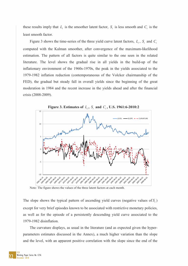
Figure 3 shows the time-series of the three yield curve latent factors, tL , tS and tC
computed with the Kalman smoother, after convergence of the maximum-likelihood
estimation. The pattern of all factors is quite similar to the one seen in the related
literature. The level shows the gradual rise in all yields in the build-up of the
inflationary environment of the 1960s-1970s, the peak in the yields associated to the
1979-1982 inflation reduction (contemporaneous of the Volcker chairmanship of the
FED), the gradual but steady fall in overall yields since the beginning of the great
moderation in 1984 and the recent increase in the yields ahead and after the financial
crisis (2008-2009).
Figure 3. Estimates of tL , tS and tC , U.S. 1961:6-2010:2
10
5
0
5
10
15
LEVEL SLOPE CURVATURE
Note: The figure shows the values of the three latent factors at each month.
The slope shows the typical pattern of ascending yield curves (negative values of tS )
except for very brief episodes known to be associated with restrictive monetary policies,
as well as for the episode of a persistently descending yield curve associated to the
1979-1982 disinflation.
The curvature displays, as usual in the literature (and as expected given the hyper-
parameters estimates discussed in the Annex), a much higher variation than the slope
and the level, with an apparent positive correlation with the slope since the end of the
23ECB
Working Paper Series No 1276December 2010
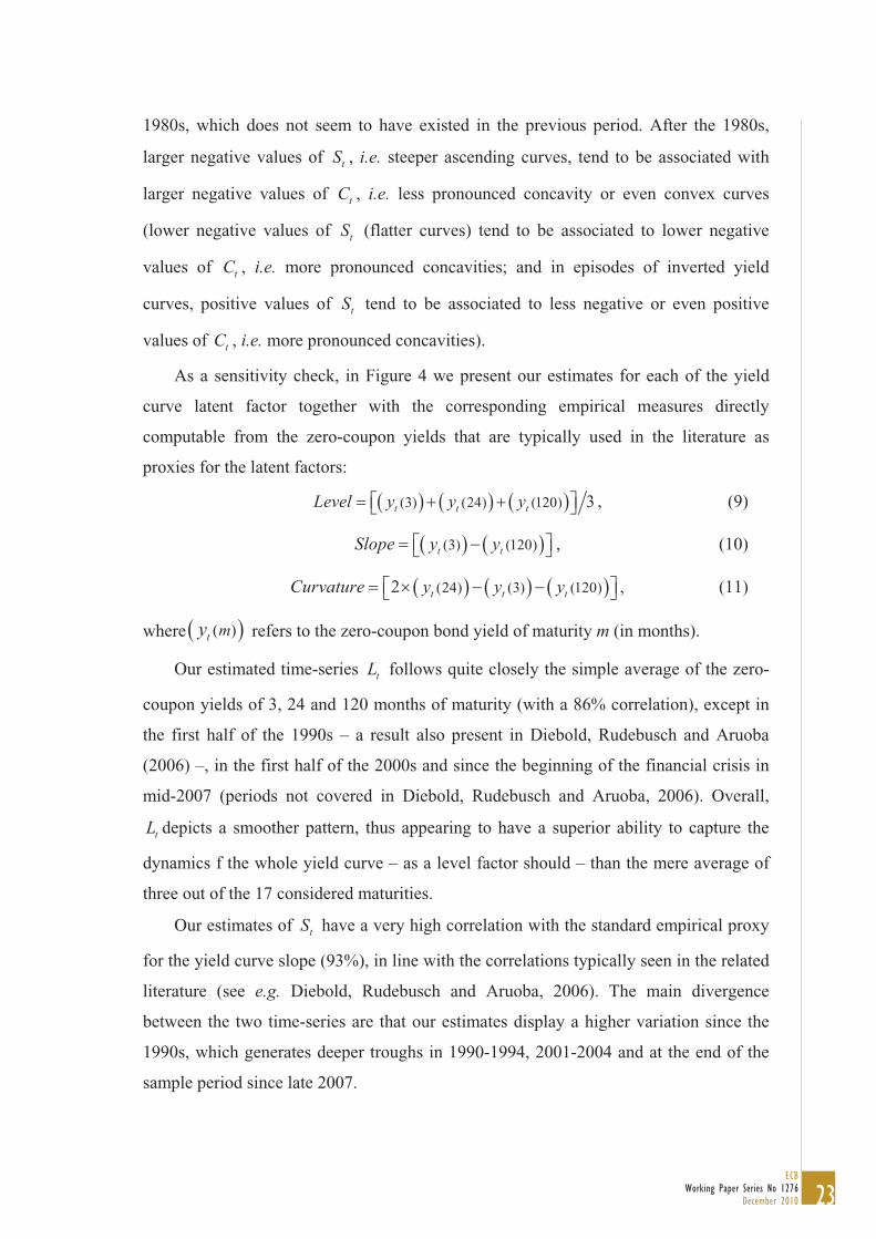
1980s, which does not seem to have existed in the previous period. After the 1980s,
larger negative values of tS , i.e. steeper ascending curves, tend to be associated with
larger negative values of tC , i.e. less pronounced concavity or even convex curves
(lower negative values of tS (flatter curves) tend to be associated to lower negative
values of tC , i.e. more pronounced concavities; and in episodes of inverted yield
curves, positive values of tS tend to be associated to less negative or even positive
values of tC , i.e. more pronounced concavities).
As a sensitivity check, in Figure 4 we present our estimates for each of the yield
curve latent factor together with the corresponding empirical measures directly
computable from the zero-coupon yields that are typically used in the literature as
proxies for the latent factors:
(3) (24) (120) 3t t tLevel y y y , (9)
(3) (120)t tSlope y y , (10)
(24) (3) (120)2 t t tCurvature y y y , (11)
where ( )t my refers to the zero-coupon bond yield of maturity m (in months).
Our estimated time-series tL follows quite closely the simple average of the zero-
coupon yields of 3, 24 and 120 months of maturity (with a 86% correlation), except in
the first half of the 1990s – a result also present in Diebold, Rudebusch and Aruoba
(2006) –, in the first half of the 2000s and since the beginning of the financial crisis in
mid-2007 (periods not covered in Diebold, Rudebusch and Aruoba, 2006). Overall,
tL depicts a smoother pattern, thus appearing to have a superior ability to capture the
dynamics f the whole yield curve – as a level factor should – than the mere average of
three out of the 17 considered maturities.
Our estimates of tS have a very high correlation with the standard empirical proxy
for the yield curve slope (93%), in line with the correlations typically seen in the related
literature (see e.g. Diebold, Rudebusch and Aruoba, 2006). The main divergence
between the two time-series are that our estimates display a higher variation since the
1990s, which generates deeper troughs in 1990-1994, 2001-2004 and at the end of the
sample period since late 2007.

24ECBWorking Paper Series No 1276December 2010
Figure 4. Estimates of tL , tS , tC , and empirical proxy, U.S. 1961:6-2010:2 4.1. Lt
0
2
4
6
8
10
12
14
16
LEVEL empirical
LEVEL
4.2. St
8
6
4
2
0
2
4
6
SLOPEempirical
SLOPE
4.3. Ct
8
6
4
2
0
2
4
6
CURVATUREempirical
CURVATURE
Note: Each chart compares, for each latent factor, the estimates obtained with maximum likelihood with the Kaman filter, as described in the text, with the corresponding empirical proxy.
25ECB
Working Paper Series No 1276December 2010
The estimated time-series for tC has a higher variability than its empirical proxy, as
Figure 4.3 clearly shows. As a result, even though their movements are fairly close to
each other, their correlation is only of 72%.
In the recent financial crisis, differently from what the empirical proxy is able to
capture, our estimates point to persistent and sizeable negative values of tC ,
corresponding to a less pronounced concavity of the yield curves, which, as shown in
Figure 4.3, were steeply upward (as monetary policy rates were decreased abruptly to
combat the crisis). Another visible difference between our tC estimates and their
empirical counterparts appear in the disinflationary episode, in which tC signals a much
more pronounced inversion of the curvature (to convexity) in association with the
inversion of the slope indicated by both tS and its proxy in Figure 4.3.
Overall, we can conclude that our estimates of the three yield curve latent factors,
tL , tS and tC , describe a historical evolution of the yield curve shape that is coherent
across the factors and consistent with the main known monetary and financial facts. The
estimates are also in line, with an apparent advantage in some episodes, with the history
described by their traditional empirical counterparts.
4.2.2. Germany
In this sub-section we present the estimates of the time-varying parameters – level,
slope and curvature – for the case of Germany. As regards hyper-parameters, as in the
U.S. case, we only discuss in the text and present further details in Annex 1 (all codes,
data and results are available from the authors upon request).
The estimate of (which is significant at 1 percent) is 0.04125, implying a
maximum of loading of the curvature at the maturity of 43 months and a rather slow
decay of the loading of the slope – a result fairly similar to the one obtained for the U.S.
Figure 5 shows the estimated time-series of tL , tS and tC (computed with the
Kalman smoother) for Germany. tL shows how Germany’s yields have peaked during
the first oil shock, given the well-known accommodative macroeconomic policy, but
also how that peak was less marked and less persistent than the one seen in the U.S. at
the end of the 1970s, given the smaller disinflation needs. The figure further shows how
yields rose after the reunification and how they have only fallen for the current standard
levels in the second half of the 1990s, ahead of the creation of the EMU.

26ECBWorking Paper Series No 1276December 2010
Figure 5. Estimates of tL , tS and tC , Germany 1972:9-2010:3
10
5
0
5
10
15
LEVEL
SLOPE
CURVATURE
Note: The figure shows the values of the three latent factors at each month.
The slope, tS , shows the typical pattern of ascending yield curves except for the
episodes known to be associated with restrictive monetary policies, as well as for the
episode of the German reunification (1991). The curvature displays, as usual, a much
higher variation than the slope and the level. As in the case of the U.S. there is an
apparent positive correlation between tS and tC since the second half of the 1980s.
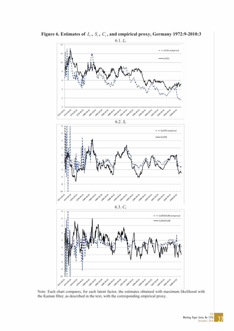
In Figure 6 we present the estimates for each of the yield curve latent factor together
with the corresponding empirical measure typically used in the literature as proxy (as in
the case of the U.S., using also equations (9), (10) and (11)). The correlations between
the model estimates and the empirical measures are somewhat smaller than for the U.S.,
which is due, mostly, to the very high volatility of the zero-coupon yields at the
beginning of the sample. For the whole sample, the correlations are of 80%, 68% and
27% respectively for the level, slope and curvature. For a sample beginning in 1980 –
such as the one that will be used in the VAR analysis (then, after computing simple
quarterly averages, to match the periodicity of the macro variables) – the correlations
are of 77%, 94% and 69%, which is more in line with the results for the U.S. case.
27ECB
Working Paper Series No 1276December 2010
Figure 6. Estimates of tL , tS , tC , and empirical proxy, Germany 1972:9-2010:3 6.1. Lt
0
2
4
6
8
10
12
14
LEVEL empirical
LEVEL
6.2. St
10
8
6
4
2
0
2
4
6
8
SLOPEempirical
SLOPE
6.3. Ct
10
8
6
4
2
0
2
4
6
8
CURVATUREempirical
CURVATURE
Note: Each chart compares, for each latent factor, the estimates obtained with maximum likelihood with the Kaman filter, as described in the text, with the corresponding empirical proxy.
28ECBWorking Paper Series No 1276December 2010
4.3. VAR analysis
It could be argued that the estimation of the yield curve latent factors and of the
macro-fiscal-finance VAR, for the sake of econometric consistency, should be
performed simultaneously in an encompassing state-space model (by maximum-
likelihood with the Kalman filter). In fact, that is the approach undertook by Diebold,
Rudebusch and Aruoba (2006) in their macro-finance empirical analysis.
Our choice of separating the state-space modelling and estimation of the yield curve
latent factors from the estimation and analysis of the macro-fiscal-finance VAR is based
on two arguments. First, subsuming the estimation of the yield curve factors and of the
VAR in a unique state-space model implies that the macro-fiscal-finance VAR is
necessarily restricted to be a VAR(1), when there is no guarantee that this would be the
outcome of the optimal lag length analysis. In fact, on the basis of the standard
information criteria and of the analysis of the autocorrelation and normality of the
residuals, we estimate a VAR(4) for the U.S. and a VAR(2) for Germany (irrespectively
of the fiscal variable). Second, the encompassing state-space model would generate
estimates of the yield curve factors that would not differ markedly from those obtained
in the pure finance state-space model described in 3.1, as only yield data are considered
in its measurement system. Thus, using the previously estimated yield curve latent
factors in a subsequent VAR analysis does not expose our framework to the generated
regressor criticism put forward by Pagan (1994).
4.3.1. U.S.
4.3.1.1. Impulse response functions
In this section we report the impulse response functions (IRFs) of all the variables in
the system to a positive innovation to the fiscal variable (annual change of the debt-to-
GDP ratio) with magnitude of one standard deviation of the respective errors, together
with the usual two-standard error (95 percent) confidence bands. Overall, the results
confirm that the system is stationary and may be summarized as follows (see Figure 7).
29ECB
Working Paper Series No 1276December 2010
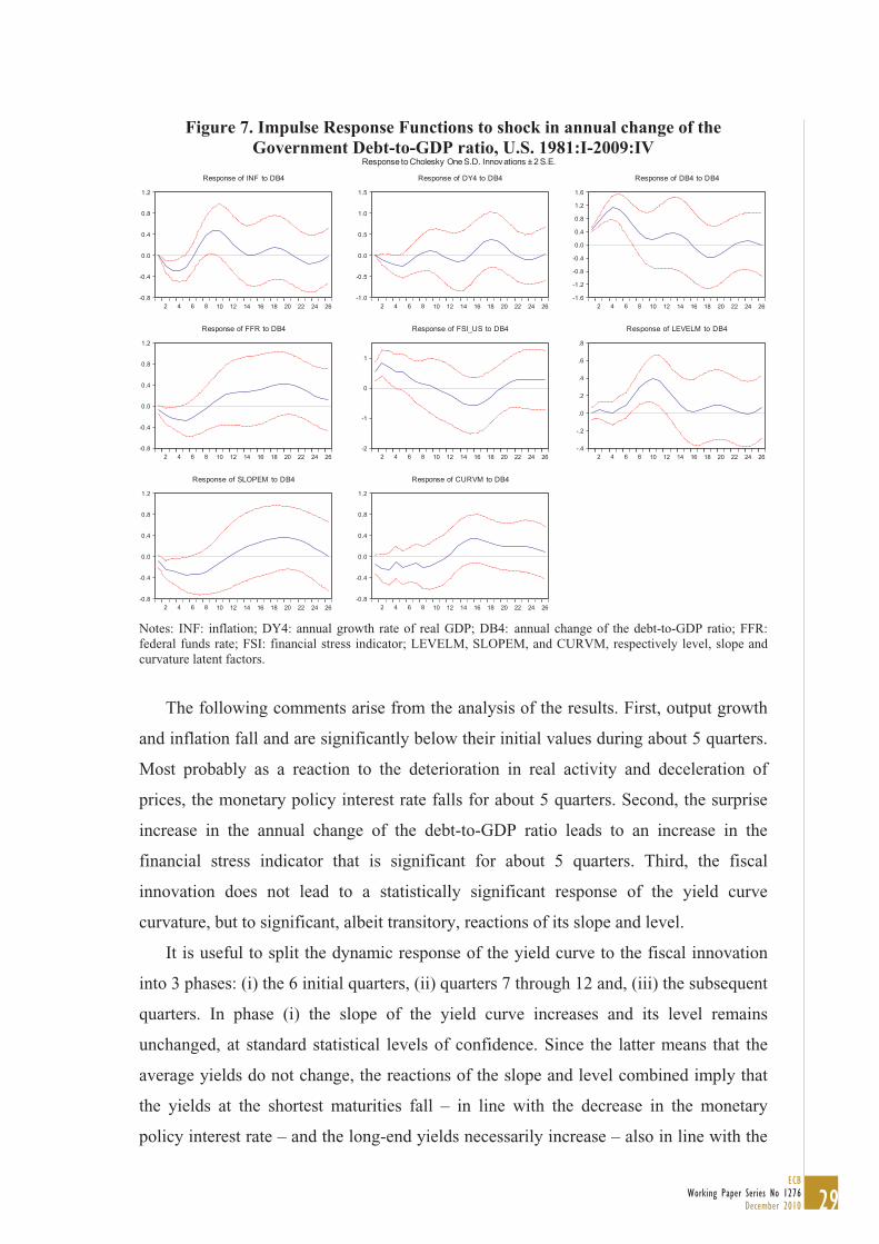
Figure 7. Impulse Response Functions to shock in annual change of the Government Debt-to-GDP ratio, U.S. 1981:I-2009:IV
-0.8
-0.4
0.0
0.4
0.8
1.2
2 4 6 8 10 12 14 16 18 20 22 24 26
Response of INF to DB4
-1.0
-0.5
0.0
0.5
1.0
1.5
2 4 6 8 10 12 14 16 18 20 22 24 26
Response of DY4 to DB4
-1.6
-1.2
-0.8
-0.4
0.0
0.4
0.8
1.2
1.6
2 4 6 8 10 12 14 16 18 20 22 24 26
Response of DB4 to DB4
-0.8
-0.4
0.0
0.4
0.8
1.2
2 4 6 8 10 12 14 16 18 20 22 24 26
Response of FFR to DB4
-2
-1
0
1
2 4 6 8 10 12 14 16 18 20 22 24 26
Response of FSI_US to DB4
-.4
-.2
.0
.2
.4
.6
.8
2 4 6 8 10 12 14 16 18 20 22 24 26
Response of LEVELM to DB4
-0.8
-0.4
0.0
0.4
0.8
1.2
2 4 6 8 10 12 14 16 18 20 22 24 26
Response of SLOPEM to DB4
-0.8
-0.4
0.0
0.4
0.8
1.2
2 4 6 8 10 12 14 16 18 20 22 24 26
Response of CURVM to DB4
Response to Cholesky One S.D. Innovations ± 2 S.E.
Notes: INF: inflation; DY4: annual growth rate of real GDP; DB4: annual change of the debt-to-GDP ratio; FFR: federal funds rate; FSI: financial stress indicator; LEVELM, SLOPEM, and CURVM, respectively level, slope and curvature latent factors.
The following comments arise from the analysis of the results. First, output growth
and inflation fall and are significantly below their initial values during about 5 quarters.
Most probably as a reaction to the deterioration in real activity and deceleration of
prices, the monetary policy interest rate falls for about 5 quarters. Second, the surprise
increase in the annual change of the debt-to-GDP ratio leads to an increase in the
financial stress indicator that is significant for about 5 quarters. Third, the fiscal
innovation does not lead to a statistically significant response of the yield curve
curvature, but to significant, albeit transitory, reactions of its slope and level.
It is useful to split the dynamic response of the yield curve to the fiscal innovation
into 3 phases: (i) the 6 initial quarters, (ii) quarters 7 through 12 and, (iii) the subsequent
quarters. In phase (i) the slope of the yield curve increases and its level remains
unchanged, at standard statistical levels of confidence. Since the latter means that the
average yields do not change, the reactions of the slope and level combined imply that
the yields at the shortest maturities fall – in line with the decrease in the monetary
policy interest rate – and the long-end yields necessarily increase – also in line with the
30ECBWorking Paper Series No 1276December 2010
deterioration in the overall financial conditions index. In phase (ii) the slope starts
falling and returns, statistically, to its original value, while the level of the yield curve
increases to values that are statistically above the initial ones, remaining so until the 12th
quarter. Combined, the reactions of the slope and of the level imply that the yields of
the short-end maturities now increase and that the yields of the long-end of the yield
curve remain above their original values. The rise in the shortest maturities yields is
consistent with the response of the monetary policy rate. Finally, from the 12th quarter
onwards, it is not possible to reject the hypothesis that the yield curve has returned to its
initial shape, i.e. the original slope and level.
In short, a positive innovation to the rate of change of the debt-to-GDP ratio leads to
an increase in the yields in the long-end maturities of the curve (which comprises, at the
extreme, the usual 10 years maturity studied in most fiscal-finance analyses) during 12
quarters, i.e. 3 years. Indeed, an innovation of 0.47 percentage points in the rate of
change of the debt ratio is associated with an upward response of the yield curve longest
maturities yields that amounts to 38 basis points, at its peak, which occurs in the 10th-
11th quarters after the innovation (a conclusion that is warranted as the values of slope
and curvature are essentially similar to their baselines).
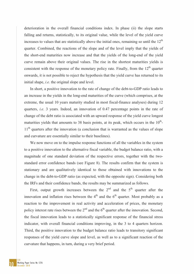
We now move on to the impulse response functions of all the variables in the system
to a positive innovation to the alternative fiscal variable, the budget balance ratio, with a
magnitude of one standard deviation of the respective errors, together with the two-
standard error confidence bands (see Figure 8). The results confirm that the system is
stationary and are qualitatively identical to those obtained with innovations to the
change in the debt-to-GDP ratio (as expected, with the opposite sign). Considering both
the IRFs and their confidence bands, the results may be summarized as follows.
First, output growth increases between the 2nd and the 5th quarter after the
innovation and inflation rises between the 4th and the 6th quarter. Most probably as a
reaction to the improvement in real activity and acceleration of prices, the monetary
policy interest rate rises between the 2nd and the 6th quarter after the innovation. Second,
the fiscal innovation leads to a statistically significant response of the financial stress
indicator, with overall financial conditions improving, in the 3 to 4 quarters horizon.
Third, the positive innovation to the budget balance ratio leads to transitory significant
responses of the yield curve slope and level, as well as to a significant reaction of the
curvature that happens, in turn, during a very brief period.
31ECB
Working Paper Series No 1276December 2010
Figure 8. Impulse Response Functions to shock in the Budget Balance, U.S. 1981:I-2009:IV
-.8
-.4
.0
.4
2 4 6 8 10 12 14 16 18 20 22 24 26
Response of INF to BALANCE
-.4
.0
.4
.8
2 4 6 8 10 12 14 16 18 20 22 24 26
Response of DY4 to BALANCE
-0.8
-0.4
0.0
0.4
0.8
1.2
2 4 6 8 10 12 14 16 18 20 22 24 26
Response of BALANCE to BALANCE
-1.2
-0.8
-0.4
0.0
0.4
0.8
2 4 6 8 10 12 14 16 18 20 22 24 26
Response of FFR to BALANCE
-1.5
-1.0
-0.5
0.0
0.5
1.0
1.5
2 4 6 8 10 12 14 16 18 20 22 24 26
Response of FSI_US to BALANCE
-.6
-.4
-.2
.0
.2
.4
2 4 6 8 10 12 14 16 18 20 22 24 26
Response of LEVELM to BALANCE
-1.0
-0.5
0.0
0.5
1.0
2 4 6 8 10 12 14 16 18 20 22 24 26
Response of SLOPEM to BALANCE
-.8
-.4
.0
.4
.8
2 4 6 8 10 12 14 16 18 20 22 24 26
Response of CURVM to BALANCE
Response to Cholesky One S.D. Innovations ± 2 S.E.
Notes: BALANCE – budget balance ratio, INF: inflation; DY4: annual growth rate of real GDP; FFR: federal funds rate; FSI: financial stress indicator; LEVELM, SLOPEM, and CURVM, respectively level, slope and curvature latent factors.
In this case we can also divide the dynamic response of the yield curve to the
balance-to-GDP ratio innovation into three phases (with the first one including a brief
sub-phase): (i) the 8 initial quarters, (ii) quarters 9 through 12, (iii) the subsequent
quarters. In phase (i) the slope of the yield curve falls and its level remains unchanged
(notice that a budget balance increase implies an improvement of the fiscal position).
The latter means that the average yields do not change and the combined reactions of
the slope and of the level imply that the yields at the shortest maturities increase – in
line with the increase in the monetary policy interest rate – and the long-end yields
necessarily fall. During quarters three through seven after the innovation, one can reject,
at 95 percent of confidence, the hypothesis that the curvature remains unchanged, in
favour of a reduction in the curvature, further reinforcing the conclusion that yields at
the long-end of the curve fall. Consistently, during a considerable part of this initial
phase, the overall financial conditions improve, in reaction to the improvement in the
fiscal position, even though the short-term interest rate increase. In phase (ii) the level is
significantly below its initial value and the slope starts increasing, as does the curvature;

32ECBWorking Paper Series No 1276December 2010
it is not possible to reject the hypothesis that the slope has returned to its original values.
These reactions of the slope and of the level mean that the yields at the short-end
maturities now decrease and that the yields of the long-end of the yield curve remain
below their original values. Finally, from the 12th quarter onwards, it is not possible to
reject the hypothesis that the yield curve has returned to its initial shape, i.e. the original
slope and level.
Summarising, a positive innovation to the budget balance (in percentage of GDP)
leads to a decrease in the yields of the long-end maturities of the curve (which
comprises, at the extreme, the usual 120 months maturity) during 12 quarters, i.e. three
years. An innovation (improvement) of 0.55 percentage points in the budget balance
ratio is associated with a downward response of the longest maturities yields that
amounts to 26 basis points in the 12th quarter after the innovation (when the slope and
the curvature have returned to their baseline values and the level component is 26 points
below its initial value).
4.3.1.2. Variance decompositions
For the case of the VAR including the change of the debt-to-GDP ratio as the fiscal
measure, the results may be summarized as follows (see Table 1). At a 4-quarter horizon
and as expected, most of the variance of the error in forecasting the change in the debt
ratio (panel 1.1) comes from fiscal innovations. However, outputs surprises and, to a
lesser extent, interest rate and inflation surprises, also explain some of that forecast error
variance. At the 8-quarter horizon, fiscal innovations account for about half of the
forecast error variance and innovations to inflation, output and the slope of the yield
curve attain a sizeable importance. For forecast horizons of 12 quarters and beyond, the
importance of surprises to the slope of the yield curve stabilizes at around 10 percent,
which corresponds to a similar explanatory power of that of output surprises (with
inflation surprises remaining the main driver of the variance of the errors in forecasting
the growth of the debt-to-GDP ratio in addition to fiscal surprises).

33ECB
Working Paper Series No 1276December 2010
Table 1. Annual Change in Debt-to-GDP Ratio Forecast Error Variance Decomposition, U.S. 1981:I-2009:IV.
1.1. Forecasting the Change of the Debt-to-GDP ratio Period INF DY4 DB4 FFR FSI L S C
4 3.644 13.426 75.805 2.119 3.834 0.245 0.781 0.142 8 24.466 9.944 49.373 2.229 4.070 0.097 8.145 1.673 12 22.251 9.633 43.444 6.011 6.411 0.206 10.131 1.910 16 22.899 9.222 42.587 5.985 6.706 0.374 10.013 2.209 20 22.641 8.705 42.060 6.374 8.233 0.442 9.361 2.181 24 22.793 8.591 39.994 6.354 9.059 0.426 10.410 2.369
1.2 Forecasting the Level of the Yield Curve Period INF DY4 DB4 FFR FSI L S C
4 1.527 15.549 0.324 0.983 1.402 73.729 1.059 5.422 8 4.491 9.898 16.469 6.3169 7.148 48.349 1.924 5.400 12 7.237 5.190 39.603 5.545 12.355 24.552 2.225 3.288 16 9.414 4.429 33.697 14.441 11.893 19.571 2.050 4.501 20 9.631 5.215 28.751 17.693 10.819 16.169 7.954 3.763 24 10.220 5.280 27.483 17.109 10.668 15.458 9.548 4.231
1.3. Forecasting the Slope of the Yield Curve Period INF DY4 DB4 FFR FSI L S C
4 0.421 8.077 12.001 38.997 0.518 12.690 27.132 0.161 8 3.108 15.146 15.901 24.509 0.472 8.292 30.944 1.626 12 6.122 13.516 14.651 21.106 1.594 6.938 33.139 2.931 16 7.140 14.060 16.208 20.375 2.442 6.077 29.783 3.913 20 8.622 14.624 20.397 17.195 2.059 5.270 27.665 4.164 24 9.695 14.367 22.463 15.85 1.978 5.069 26.581 3.988
1.4. Forecasting the Curvature of the Yield Curve Period INF DY4 DB4 FFR FSI L S C
4 2.959 16.937 5.614 0.521 13.713 3.906 11.182 45.164 8 4.979 20.379 7.771 0.419 11.369 6.069 13.641 35.370 12 5.222 19.769 8.659 0.544 10.640 6.797 15.529 32.837 16 5.693 17.267 15.400 0.510 12.157 5.975 14.371 28.624 20 7.845 16.014 18.484 1.258 11.065 5.342 13.179 26.810 24 7.521 15.297 20.295 2.787 10.609 5.214 12.635 25.640
Notes: INF: inflation; DY4: annual growth rate of real GDP; DB4: annual change of the debt-to-GDP ratio; FFR: federal funds rate; FSI: financial stress indicator; L: level of the yield curve; S: slope of the yield curve; C: curvature of the yield curve. Each row shows the percentage of the variance of the error in forecasting the variable mentioned in the title of the table, at each forecasting horizon (in quarters) given in the first column.
As panel 1.2 in Table 1 shows, the variance of the errors in forecasting the level of
the yield curve at a 4-quarter horizon is mostly explained, as expected, by innovations
to the level itself. Nevertheless, surprises to output growth and, although to a lesser
extent, surprises to the curvature of the yield curve explain sizeable parts of such
variance. From the 8-quarter horizon onwards, innovations to the change in the debt-to-
GDP ratio become the most important explanations for the variance of the errors in
forecasting the yield curve level (from the 12-quarter horizon onwards even above
innovations to the level itself). This contribution peaks at almost 40 percent in the 12
quarters horizon and is still around 28 percent at the horizon of six years. From the 8th
quarter onwards the shocks to the financial stress indicator also account for around 12
34ECBWorking Paper Series No 1276December 2010
percent of the forecast error variance of the level of the yield curve and from the 16-
quarter horizon monetary policy surprises account for more than 15 per cent of the error
variance. Most importantly, fiscal surprises account for a much larger fraction of the
forecast error variance of the yield curve level than any individual macroeconomic and
financial variables.
Panel 1.3 in Table 1 shows that in a 4-quarter horizon, surprises to the monetary
policy interest rate explain the major part of the variance of the forecasting errors of the
yield curve slope – a result that is consistent with the monetary policy hypothesis
regarding the power of the yield curve slope to predict economic activity. As the
forecast horizon widens, the part explained by monetary policy innovations falls
gradually, but remains as large as 15 percent at a 24 quarters horizon. From the 8-
quarter horizon onwards, surprises to the growth rate of real GDP explain a sizeable part
of the slope forecast error variance, as well as do surprises to inflation, albeit with a
delay and smaller magnitudes. Innovations to the government debt ratio explain a bit
less than they do in the case of the forecast error variance of the level, but are still very
much considerable in the case of the yield curve slope, and increase their contribution
gradually as the forecast horizon widens, from 15 percent at the 8-quarter horizon to 22
percent at the 24-quarter horizon.
Finally, panel 1.4 in Table 1 shows that at a 4-quarter horizon, surprises to the yield
curve curvature itself explain the largest part of the forecast error variance of the
curvature, as expected, but that surprises to real output growth and the financial stress
index also have important explanatory power, as also have surprises to the yield curve
slope. While fiscal surprises initially do not explain a considerable part of the curvature
forecast error variance, their importance increases steadily with the forecast horizon and
amounts to 15 to 20 percent at horizons above 16 quarters. Innovations to the yield
curve slope have similar explanatory power as do surprises to the overall financial
conditions index.
We now move to the decomposition of the forecast errors variance for the balance-
to-GDP ratio and the yield curve latent factors, for the selected horizons above
considered for the case of the alternative fiscal policy variable. The results can be
summarized as follows (see Table 2).

35ECB
Working Paper Series No 1276December 2010
Table 2. Balance Forecast Error Variance Decomposition, U.S. 1981:I-2009:IV. 2.1. Forecasting the Budget Balance
Period INF DY4 BALANCE FFR FSI L S C 4 2.018 5.984 69.998 0.470 10.578 3.433 7.091 0.429 8 3.592 7.049 65.332 0.839 7.131 3.116 12.776 0.166 12 3.327 7.286 60.621 4.909 7.282 2.226 14.238 0.110 16 3.615 6.950 58.149 7.363 9.061 1.938 12.803 0.121 20 3.749 6.853 56.329 9.417 9.184 1.898 12.106 0.462 24 3.777 6.868 55.243 10.289 9.448 1.987 11.600 0.788
2.2 Forecasting the Level of the Yield Curve Period INF DY4 BALANCE FFR FSI L S C
4 1.653 19.183 0.771 1.016 2.027 68.705 1.314 5.330 8 10.873 12.876 2.946 4.109 15.703 46.076 1.493 5.924 12 7.506 7.296 17.151 6.293 30.553 25.656 1.263 4.282 16 6.196 5.694 20.448 17.717 24.903 19.414 1.211 4.417 20 5.937 4.963 18.873 21.355 24.972 16.662 2.771 4.467 24 5.998 4.717 21.299 21.124 24.010 14.925 2.810 5.118
2.3. Forecasting the Slope of the Yield Curve Period INF DY4 BALANCE FFR FSI L S C
4 1.548 6.634 15.905 34.293 0.038 15.055 26.373 0.151 8 1.049 10.52 25.401 18.450 2.383 10.329 28.939 2.921 12 2.199 9.067 26.615 15.772 2.423 8.501 30.610 4.809 16 2.410 9.054 26.574 16.592 2.444 8.288 29.658 4.978 20 2.325 9.219 28.243 15.492 2.522 7.972 29.568 4.656 24 2.353 9.116 29.462 14.998 3.111 7.581 28.878 4.498
2.4. Forecasting the Curvature of the Yield Curve Period INF DY4 BALANCE FFR FSI L S C
4 1.958 13.717 11.621 1.304 17.147 2.221 7.461 44.567 8 6.343 15.293 16.442 1.123 14.758 3.529 7.738 34.771 12 6.433 15.211 15.986 1.823 15.763 4.171 8.439 32.170 16 6.534 13.446 18.113 2.131 20.086 3.733 7.346 28.606 20 5.569 11.568 23.562 3.298 21.093 3.309 6.107 25.491 24 5.208 10.707 24.948 6.001 19.468 3.127 5.559 24.979
Notes: INF - inflation; DY4 - annual growth rate of real GDP; BALANCE - budget balance in percentage of GDP; FFR - federal funds rate; FSI - financial stress indicator; L - level of the yield curve; S - slope of the yield curve; C - curvature of the yield curve. Each row shows the percentage of the variance of the error in forecasting the variable mentioned in the title of the table, at each forecasting horizon (in quarters) given in the first column.
At a 4-quarter horizon, most of the variance of the error in forecasting the budget
balance-to-GDP ratio arises naturally from the fiscal innovations (panel 2.1 in Table 2).
However, surprises to the financial stress indicator, and, to a lesser extent, output
surprises, also explain some of that forecast error variance. Most importantly,
innovations to the yield curve slope explain around 7 percent of the variance of the error
in forecasting the balance. At a horizon of eight quarters, fiscal innovations still account
for about two thirds of the forecast error variance, while innovations to output, financial
conditions and, with increasing weight, innovations to the slope of the yield curve attain
a sizeable importance. For forecast horizons of 12 quarters and beyond, surprises to the
slope of the yield curve are the larger explanation for the forecast error variance
(stabilizing at around 12 percent), even though innovations to the interest rate, financial

36ECBWorking Paper Series No 1276December 2010
conditions and output growth gradually gain some importance in explaining the
variance of errors in forecasting the balance-to-GDP ratio.
As can be seem in panel 2.2 of Table 2, the variance of the errors in forecasting the
level of the yield curve at a 4-quarter horizon is mostly explained, as expected, by
innovations to the level itself. Although to a lesser extent, surprises to output growth
and to the curvature of the yield curve also explain sizeable parts of such variance.
These features are quite similar to those seen in the case of the growth of the debt-to-
GDP ratio. At the 8, 12 and 16 quarters horizons, innovations to the FSI become the
most important explanations for the variance of the errors in forecasting the yield curve
level. The explanatory importance of the budget balance ratio increases steadily along
the forecast horizon, and while it is still inferior to those of output and inflation
surprises at the 8 quarters horizon, it becomes more important at the 12 quarter horizon,
and almost as relevant an explanation for the errors in forecasting the level of the yield
curve at the 16, 20 and 24 quarters horizon as the financial conditions index. Its
explanatory power peaks somewhat later and at a lower proportion than it is the case of
the government debt ratio (see panel 2.2 in Table 2). Most importantly, after the 16
quarters horizon, fiscal surprises and the financial stress indicator surprises account for
a much larger fraction of the forecast error variance of the yield curve level than the
macroeconomic variables, inflation and output, as well as, broadly, the monetary policy
interest rate.
Regarding the variance of the forecasting errors of the yield curve slope, they are
mainly explained by surprises to the monetary policy interest rate at a 4-quarter horizon
(see panel 2.3 of Table 2). Yet, surprises in the budget ratio and in the level of the yield
curve explain a considerable proportion of the forecast error variance. Moreover, as the
forecast horizon widens to no less than 8 quarters, surprises to the fiscal balance
consistently are the larger explaining factor for the variance of the errors in forecasting
the yield curve slope, besides surprises to the slope itself, which makes fiscal policy the
main explanation for errors in forecasting the slope. In fact, surprises to the monetary
policy innovations keep on having a considerable role, but their contribution is much
smaller than in the case of the model with government debt. In turn, surprises to real
output growth have a similar importance. In comparison to what happens for the model
with the debt ratio, in the specification including the budget balance ratio, fiscal
innovations explain much more of the forecast error variance of the slope than of the
level.

37ECB
Working Paper Series No 1276December 2010
Finally, panel 2.4 of Table 2 reports that at a 4-quarter horizon, surprises to the yield
curve curvature itself explain the largest part of the forecast error variance of the
curvature, as expected, but that surprises to real output growth and the financial stress
index also have important explanatory power. In comparison to what is seen in the
system including the growth in the debt-to-GDP ratio, here surprises to the yield curve
slope have a more limited explanatory power of the variance of the forecast errors of the
curvature. Budget balance surprises explain a considerable part of the curvature forecast
error variance, and their importance increases steadily with the forecast horizon and
amounts to 24 percent at horizons above 20 quarters. At horizons beyond the 4 quarters,
surprises to the fiscal balance explain overall a larger part of the forecast error variance
of the curvature than do surprises to real output growth and to the financial stress
indicator.
4.3.1.3. Granger causality
In this section we present results for Granger causality tests between the fiscal
variables and the yield curve latent factors. We have run the tests for two lag lengths,
motivated by the analysis of the IRFs above. First, we have included four lags of all
regressors, which is the lag length considered in the estimation of the VARs and should
allow for capturing the most immediate inter-relations between fiscal and yield curve
variables. Then, we have run the tests including 12 lags of all the regressors, the horizon
after which, according to the IRFs, both the slope and the level of the yield curve return
to their original values following fiscal innovations.
Table 3 (panel 3.1) shows that lags of the change in the debt-to-GDP ratio fail to
statistically decrease the variance of the error in regressions explaining each and all of
the yield curve factors, either at the 4-quarter and at the 12-quarter horizons. However,
the results shows that the yield curve slope is a leading indicator of the change in the
debt-to-GDP ratio once an horizon beyond the first 4 quarters is considered –
specifically with a p-value of 3.9 percent within the 12-quarters horizon. In such an
extended horizon, the slope improves the prediction of the yield curve level, in addition
to purely autoregressive predictions, with a p-value of 2.8 percent. For both horizons
considered, the curvature Granger-causes the yield curve level, at standard significance
levels.

38ECBWorking Paper Series No 1276December 2010
Table 3. Granger Causality between the fiscal variables and the Yield Curve latent factors, U.S. 1981:I-2009:IV 3.1. Debt-to-GDP ratio
Lags in regressions: 4 Lags in regressions: 12 DB4 L S C DB4 L S C
DB4 --- 0.486 0.148 0.882 --- 0.158 0.345 0.696 L 0.231 --- 0.019** 0.129 0.266 --- 0.063* 0.335 S 0.151 0.177 --- 0.962 0.039** 0.028** --- 0.217 C 0.155 0.014** 0.184 --- 0.673 0.081* 0.676 ---
3.2. Budget balanceLags in regressions: 4 Lags in regressions: 12
BALANCE L S C BALANCE L S C BALANCE --- 0.650 0.019** 0.031** --- 0.311 0.199 0.003***
L 0.601 --- 0.019** 0.129 0.445 --- 0.063* 0.335 S 0.153 0.173 --- 0.962 0.486 0.028** --- 0.217 C 0.401 0.014** 0.184 --- 0.950 0.081* 0.676 ---
Notes: DB4: annual change of the debt-to-GDP ratio; BALANCE - fiscal deficit in percentage of GDP; L - level of the yield curve; S - slope of the yield curve; C - curvature of the yield curve. Each entry shows the p-value for the rejection of the null hypothesis that the variable in each row does not Granger-cause the variable in each column (Significance levels: *** 1 percent; ** 5 percent; * 10 percent.).
We now move to the results for Granger causality tests between the budget balance
and the yield curve latent factors, again for both 4 and 12 lag lengths (panel 3.2 of Table
3). The results are somewhat different from those obtained with the debt ratio. For a
horizon of four lags the budget balance ratio significantly decreases the variance of the
error in auto-regressions of the yield curve slope (p-value of 0.2 percent) and curvature
(p-value of 3.1 percent). Such a result holds, in regressions including 12 lags, for the
case of the curvature, but not of the slope. The results further show that none of the
yield curve latent factors Granger-causes the budget balance ratio, at acceptable
significance levels. Finally, while the slope is a leading indicator of the yield curve
level, but only when the regressions are extended up to 12 lags (p-value of 2.8 percent),
the curvature is a leading indicator of the yield curve slope irrespectively of the
extension of the regressions (although with a somehow high p-value of 8 percent for the
12 lag regressions).
4.3.2. Germany
In this section we describe the results of the VAR analyses for the case of Germany.
As in the previous sub-section, for the U.S. case, we report results for two VARs, each
with an alternative measure of fiscal developments – the annual change in the
government-to-GDP ratio and the budget balance ratio – sequentially looking at the
impulse response functions, variance decomposition and Granger causality.
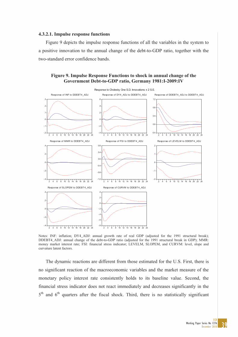
39ECB
Working Paper Series No 1276December 2010
4.3.2.1. Impulse response functions
Figure 9 depicts the impulse response functions of all the variables in the system to
a positive innovation to the annual change of the debt-to-GDP ratio, together with the
two-standard error confidence bands.
Figure 9. Impulse Response Functions to shock in annual change of the Government Debt-to-GDP ratio, Germany 1981:I-2009:IV
-.2
-.1
.0
.1
.2
.3
2 4 6 8 10 12 14 16 18 20 22 24
Response of INF to DDEBT4_ADJ
-.4
-.2
.0
.2
.4
.6
2 4 6 8 10 12 14 16 18 20 22 24
Response of DY4_ADJ to DDEBT4_ADJ
-0.4
0.0
0.4
0.8
1.2
2 4 6 8 10 12 14 16 18 20 22 24
Response of DDEBT4_ADJ to DDEBT4_ADJ
-.4
-.2
.0
.2
.4
2 4 6 8 10 12 14 16 18 20 22 24
Response of MMR to DDEBT4_ADJ
-1.2
-0.8
-0.4
0.0
0.4
0.8
2 4 6 8 10 12 14 16 18 20 22 24
Response of FSI to DDEBT4_ADJ
-.2
-.1
.0
.1
.2
2 4 6 8 10 12 14 16 18 20 22 24
Response of LEVELM to DDEBT4_ADJ
-.4
-.2
.0
.2
.4
2 4 6 8 10 12 14 16 18 20 22 24
Response of SLOPEM to DDEBT4_ADJ
-.8
-.6
-.4
-.2
.0
.2
.4
2 4 6 8 10 12 14 16 18 20 22 24
Response of CURVM to DDEBT4_ADJ
Response to Cholesky One S.D. Innovations ± 2 S.E.
Notes: INF: inflation; DY4_ADJ: annual growth rate of real GDP (adjusted for the 1991 structural break); DDEBT4_ADJ: annual change of the debt-to-GDP ratio (adjusted for the 1991 structural break in GDP); MMR: money market interest rate; FSI: financial stress indicator; LEVELM, SLOPEM, and CURVM: level, slope and curvature latent factors.
The dynamic reactions are different from those estimated for the U.S. First, there is
no significant reaction of the macroeconomic variables and the market measure of the
monetary policy interest rate consistently holds to its baseline value. Second, the
financial stress indicator does not react immediately and decreases significantly in the
5th and 6th quarters after the fiscal shock. Third, there is no statistically significant
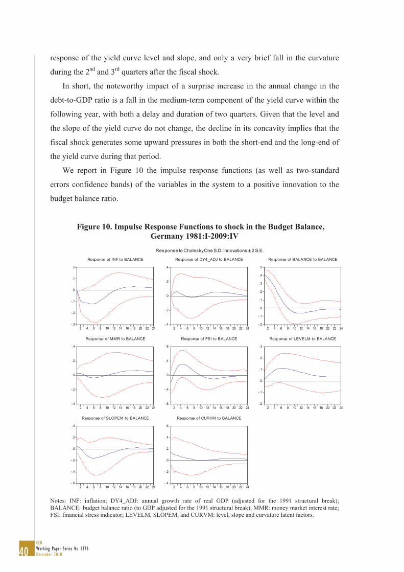
40ECBWorking Paper Series No 1276December 2010
response of the yield curve level and slope, and only a very brief fall in the curvature
during the 2nd and 3rd quarters after the fiscal shock.
In short, the noteworthy impact of a surprise increase in the annual change in the
debt-to-GDP ratio is a fall in the medium-term component of the yield curve within the
following year, with both a delay and duration of two quarters. Given that the level and
the slope of the yield curve do not change, the decline in its concavity implies that the
fiscal shock generates some upward pressures in both the short-end and the long-end of
the yield curve during that period.
We report in Figure 10 the impulse response functions (as well as two-standard
errors confidence bands) of the variables in the system to a positive innovation to the
budget balance ratio.
Figure 10. Impulse Response Functions to shock in the Budget Balance, Germany 1981:I-2009:IV
-.3
-.2
-.1
.0
.1
.2
2 4 6 8 10 12 14 16 18 20 22 24
Response of INF to BALANCE
-.4
-.2
.0
.2
.4
2 4 6 8 10 12 14 16 18 20 22 24
Response of DY4_ADJ to BALANCE
-.2
-.1
.0
.1
.2
.3
.4
.5
2 4 6 8 10 12 14 16 18 20 22 24
Response of BALANCE to BALANCE
-.4
-.2
.0
.2
.4
2 4 6 8 10 12 14 16 18 20 22 24
Response of MMR to BALANCE
-.8
-.4
.0
.4
.8
2 4 6 8 10 12 14 16 18 20 22 24
Response of FSI to BALANCE
-.2
-.1
.0
.1
.2
.3
2 4 6 8 10 12 14 16 18 20 22 24
Response of LEVELM to BALANCE
-.6
-.4
-.2
.0
.2
.4
2 4 6 8 10 12 14 16 18 20 22 24
Response of SLOPEM to BALANCE
-.4
-.2
.0
.2
.4
.6
2 4 6 8 10 12 14 16 18 20 22 24
Response of CURVM to BALANCE
Response to Cholesky One S.D. Innovations ± 2 S.E.
Notes: INF: inflation; DY4_ADJ: annual growth rate of real GDP (adjusted for the 1991 structural break); BALANCE: budget balance ratio (to GDP adjusted for the 1991 structural break); MMR: money market interest rate; FSI: financial stress indicator; LEVELM, SLOPEM, and CURVM: level, slope and curvature latent factors.
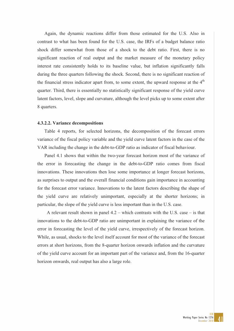
41ECB
Working Paper Series No 1276December 2010
Again, the dynamic reactions differ from those estimated for the U.S. Also in
contrast to what has been found for the U.S. case, the IRFs of a budget balance ratio
shock differ somewhat from those of a shock to the debt ratio. First, there is no
significant reaction of real output and the market measure of the monetary policy
interest rate consistently holds to its baseline value, but inflation significantly falls
during the three quarters following the shock. Second, there is no significant reaction of
the financial stress indicator apart from, to some extent, the upward response at the 4th
quarter. Third, there is essentially no statistically significant response of the yield curve
latent factors, level, slope and curvature, although the level picks up to some extent after
8 quarters.
4.3.2.2. Variance decompositions
Table 4 reports, for selected horizons, the decomposition of the forecast errors
variance of the fiscal policy variable and the yield curve latent factors in the case of the
VAR including the change in the debt-to-GDP ratio as indicator of fiscal behaviour.
Panel 4.1 shows that within the two-year forecast horizon most of the variance of
the error in forecasting the change in the debt-to-GDP ratio comes from fiscal
innovations. These innovations then lose some importance at longer forecast horizons,
as surprises to output and the overall financial conditions gain importance in accounting
for the forecast error variance. Innovations to the latent factors describing the shape of
the yield curve are relatively unimportant, especially at the shorter horizons; in
particular, the slope of the yield curve is less important than in the U.S. case.
A relevant result shown in panel 4.2 – which contrasts with the U.S. case – is that
innovations to the debt-to-GDP ratio are unimportant in explaining the variance of the
error in forecasting the level of the yield curve, irrespectively of the forecast horizon.
While, as usual, shocks to the level itself account for most of the variance of the forecast
errors at short horizons, from the 8-quarter horizon onwards inflation and the curvature
of the yield curve account for an important part of the variance and, from the 16-quarter
horizon onwards, real output has also a large role.
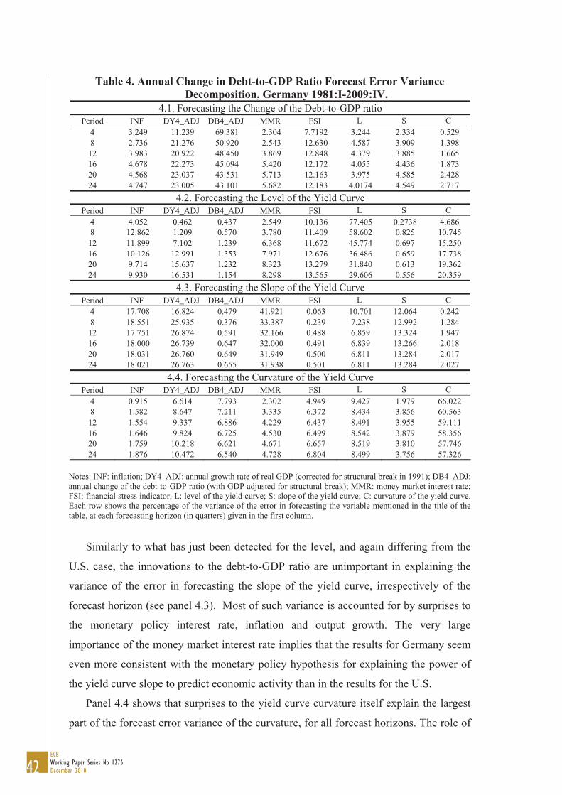
42ECBWorking Paper Series No 1276December 2010
Table 4. Annual Change in Debt-to-GDP Ratio Forecast Error Variance Decomposition, Germany 1981:I-2009:IV.
4.1. Forecasting the Change of the Debt-to-GDP ratio Period INF DY4_ADJ DB4_ADJ MMR FSI L S C
4 3.249 11.239 69.381 2.304 7.7192 3.244 2.334 0.529 8 2.736 21.276 50.920 2.543 12.630 4.587 3.909 1.398 12 3.983 20.922 48.450 3.869 12.848 4.379 3.885 1.665 16 4.678 22.273 45.094 5.420 12.172 4.055 4.436 1.873 20 4.568 23.037 43.531 5.713 12.163 3.975 4.585 2.428 24 4.747 23.005 43.101 5.682 12.183 4.0174 4.549 2.717
4.2. Forecasting the Level of the Yield Curve Period INF DY4_ADJ DB4_ADJ MMR FSI L S C
4 4.052 0.462 0.437 2.549 10.136 77.405 0.2738 4.686 8 12.862 1.209 0.570 3.780 11.409 58.602 0.825 10.745 12 11.899 7.102 1.239 6.368 11.672 45.774 0.697 15.250 16 10.126 12.991 1.353 7.971 12.676 36.486 0.659 17.738 20 9.714 15.637 1.232 8.323 13.279 31.840 0.613 19.362 24 9.930 16.531 1.154 8.298 13.565 29.606 0.556 20.359
4.3. Forecasting the Slope of the Yield Curve Period INF DY4_ADJ DB4_ADJ MMR FSI L S C
4 17.708 16.824 0.479 41.921 0.063 10.701 12.064 0.242 8 18.551 25.935 0.376 33.387 0.239 7.238 12.992 1.284 12 17.751 26.874 0.591 32.166 0.488 6.859 13.324 1.947 16 18.000 26.739 0.647 32.000 0.491 6.839 13.266 2.018 20 18.031 26.760 0.649 31.949 0.500 6.811 13.284 2.017 24 18.021 26.763 0.655 31.938 0.501 6.811 13.284 2.027
4.4. Forecasting the Curvature of the Yield Curve Period INF DY4_ADJ DB4_ADJ MMR FSI L S C
4 0.915 6.614 7.793 2.302 4.949 9.427 1.979 66.022 8 1.582 8.647 7.211 3.335 6.372 8.434 3.856 60.563 12 1.554 9.337 6.886 4.229 6.437 8.491 3.955 59.111 16 1.646 9.824 6.725 4.530 6.499 8.542 3.879 58.356 20 1.759 10.218 6.621 4.671 6.657 8.519 3.810 57.746 24 1.876 10.472 6.540 4.728 6.804 8.499 3.756 57.326
Notes: INF: inflation; DY4_ADJ: annual growth rate of real GDP (corrected for structural break in 1991); DB4_ADJ:annual change of the debt-to-GDP ratio (with GDP adjusted for structural break); MMR: money market interest rate; FSI: financial stress indicator; L: level of the yield curve; S: slope of the yield curve; C: curvature of the yield curve. Each row shows the percentage of the variance of the error in forecasting the variable mentioned in the title of the table, at each forecasting horizon (in quarters) given in the first column.
Similarly to what has just been detected for the level, and again differing from the
U.S. case, the innovations to the debt-to-GDP ratio are unimportant in explaining the
variance of the error in forecasting the slope of the yield curve, irrespectively of the
forecast horizon (see panel 4.3). Most of such variance is accounted for by surprises to
the monetary policy interest rate, inflation and output growth. The very large
importance of the money market interest rate implies that the results for Germany seem
even more consistent with the monetary policy hypothesis for explaining the power of
the yield curve slope to predict economic activity than in the results for the U.S.
Panel 4.4 shows that surprises to the yield curve curvature itself explain the largest
part of the forecast error variance of the curvature, for all forecast horizons. The role of
43ECB
Working Paper Series No 1276December 2010
innovations to changes in the debt-to-GDP ratio in accounting for the variance of the
error in forecasting the curvature is far larger than their role in accounting for the
forecast error of the other two latent factors of the yield curve, but is still rather limited
as it amounts to less than 8 percent (at the 4-quarter horizon).
We report in Table 5 the decomposition of the forecast errors variance of the budget
balance ratio and the yield curve latent factors, for the same selected horizons.
As panel 5.1 shows, at the 4-quarter horizon most of the variance of the error in
forecasting the budget balance-to-GDP ratio arises from the fiscal innovations, but from
the 8-quarter horizon onwards surprises to the financial stress indicator and to output
explain considerable parts of that forecast error variance. At horizons between 8 and 16
quarters, innovations to the level and the slope of the yield curve together explain
around 13 percent of the variance of the error in forecasting the budget balance, and
while their importance slightly decreases from the 20-quarters horizon on, the curvature
gains importance and the yield curve factors account for 18 percent of the error
variance.
Innovations to the level of the yield curve are the larger explanation for the variance
of the error in forecasting the level itself, but the financial stress index and the curvature
of the yield curve are also important explanatory factors (as well as output growth, after
the 16 quarter-horizon – see panel 5.2). Moreover, innovations to the budget balance
ratio are moderately important in accounting for the variance of the error in forecasting
the level of the yield curve, recording a degree of relevance similar to that of inflation
and a bit higher than that of the monetary policy interest rate (until the 16-quarter
horizon).
In addition, and as panel 5.3 shows, innovations to the budget balance are
unimportant in accounting for the variance of the forecasting errors of the yield curve
slope – which contrasts, as happened with the debt ratio, with the results for the U.S.
Most of that variance is explained by innovations to output growth and by innovations
to the monetary policy interest rate, as well as, to a smaller but constant extent, by
surprises to the slope itself and inflation.
Finally, panel 5.4 shows that innovations to the budget balance ratio are unimportant
in accounting for the variance of the forecast errors of the yield curve curvature. Such
findings differ from the U.S. case and, for this particular yield curve latent factor, are
also in contrast to what has been found in the previous VAR, with the change in the
debt ratio as fiscal indicator for Germany. Innovations to the yield curve curvature itself

44ECBWorking Paper Series No 1276December 2010
explain, by and large, the bulk of the forecast error variance of the curvature. As regards
the remaining variables, only surprises to the yield curve level, output growth and, to a
lesser extent, the financial stress index, accounts for non-trivial parts of that error
variance.
Table 5. Budget Balance Forecast Error Variance Decomposition, Germany 1981:I-2009:IV.
5.1. Forecasting the Budget Balance Period INF DY4_ADJ BALANCE MMR FSI L S C
4 2.046 11.696 71.119 1.284 4.906 3.136 5.731 0.082 8 2.501 18.959 47.488 1.209 15.252 5.554 8.674 0.362 12 2.807 18.437 44.129 4.325 15.306 5.827 8.258 0.911 16 2.914 21.343 38.076 7.244 14.145 5.216 8.229 2.833 20 2.735 23.365 34.359 7.965 14.153 4.976 7.932 4.516 24 3.181 23.634 32.907 7.934 14.231 5.011 7.611 5.491
5.2. Forecasting the Level of the Yield Curve Period INF DY4_ADJ BALANCE MMR FSI L S C
4 2.639 0.588 3.317 2.575 10.817 76.019 0.379 3.666 8 9.617 1.104 7.608 3.836 12.731 55.104 0.815 9.186 12 8.636 6.484 8.169 6.121 13.994 42.128 0.651 13.816 16 7.430 11.906 7.237 7.468 15.275 33.869 0.638 16.177 20 7.312 14.564 6.506 7.898 15.812 29.753 0.585 17.571 24 7.626 15.621 6.145 7.960 16.033 27.625 0.530 18.462
5.3. Forecasting the Slope of the Yield Curve Period INF DY4_ADJ BALANCE MMR FSI L S C
4 13.529 17.972 0.821 42.745 0.152 10.975 13.064 0.742 8 13.714 28.237 2.647 32.952 0.140 7.172 13.186 1.952 12 13.159 29.348 3.171 31.757 0.154 6.771 13.117 2.522 16 13.680 29.091 3.170 31.474 0.169 6.713 13.081 2.622 20 13.785 29.030 3.192 31.408 0.171 6.684 13.116 2.616 24 13.780 29.022 3.207 31.402 0.178 6.681 13.116 2.615
5.4. Forecasting the Curvature of the Yield Curve Period INF DY4_ADJ BALANCE MMR FSI L S C
4 0.587 6.763 1.182 2.094 4.764 11.097 2.261 71.252 8 1.148 8.939 1.104 3.088 6.148 9.861 4.092 65.621 12 1.156 9.764 1.057 4.207 6.139 9.731 4.144 63.803 16 1.275 10.360 1.064 4.568 6.169 9.653 4.046 62.866 20 1.411 10.751 1.114 4.696 6.345 9.577 3.966 62.140 24 1.533 10.988 1.153 4.744 6.535 9.525 3.907 61.615
Notes: INF: inflation; DY4_ADJ: annual growth rate of real GDP (adjusted for the 1991 structural break); BALANCE: budget balance ratio (to GDP adjusted for the 1991 structural break); MMR: money market interest rate; FSI: financial stress indicator; L: level of the yield curve; S: slope of the yield curve; C: curvature of the yield curve. Each row shows the percentage of the variance of the error in forecasting the variable mentioned in the title of the table, at each forecasting horizon (in quarters) given in the first column.
4.3.2.3. Granger causality
In Table 6 we summarize the results of Granger causality tests between the fiscal
variables and the yield curve latent factors in the case of Germany. Similarly to the U.S.
case, we have run the tests for two lag lengths, the first corresponding to the order of the
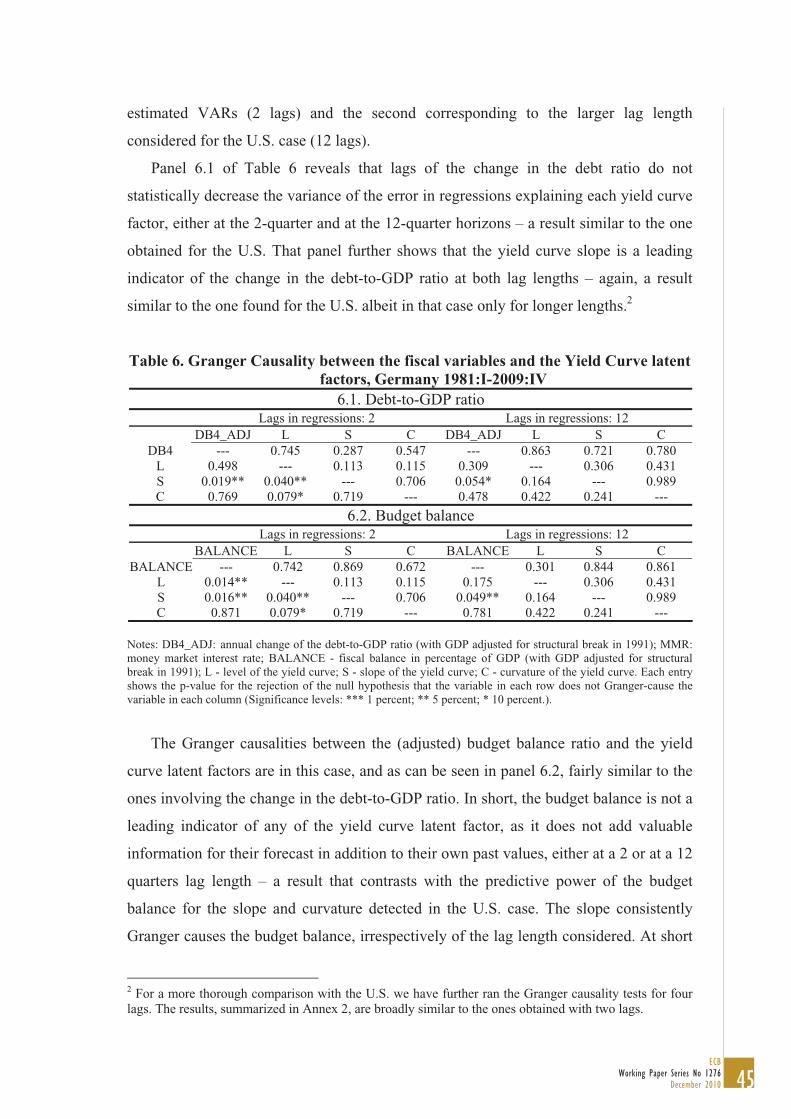
45ECB
Working Paper Series No 1276December 2010
estimated VARs (2 lags) and the second corresponding to the larger lag length
considered for the U.S. case (12 lags).
Panel 6.1 of Table 6 reveals that lags of the change in the debt ratio do not
statistically decrease the variance of the error in regressions explaining each yield curve
factor, either at the 2-quarter and at the 12-quarter horizons – a result similar to the one
obtained for the U.S. That panel further shows that the yield curve slope is a leading
indicator of the change in the debt-to-GDP ratio at both lag lengths – again, a result
similar to the one found for the U.S. albeit in that case only for longer lengths.2
Table 6. Granger Causality between the fiscal variables and the Yield Curve latent factors, Germany 1981:I-2009:IV
6.1. Debt-to-GDP ratio Lags in regressions: 2 Lags in regressions: 12 DB4_ADJ L S C DB4_ADJ L S C
DB4 --- 0.745 0.287 0.547 --- 0.863 0.721 0.780 L 0.498 --- 0.113 0.115 0.309 --- 0.306 0.431 S 0.019** 0.040** --- 0.706 0.054* 0.164 --- 0.989 C 0.769 0.079* 0.719 --- 0.478 0.422 0.241 ---
6.2. Budget balanceLags in regressions: 2 Lags in regressions: 12
BALANCE L S C BALANCE L S C BALANCE --- 0.742 0.869 0.672 --- 0.301 0.844 0.861
L 0.014** --- 0.113 0.115 0.175 --- 0.306 0.431 S 0.016** 0.040** --- 0.706 0.049** 0.164 --- 0.989 C 0.871 0.079* 0.719 --- 0.781 0.422 0.241 ---
Notes: DB4_ADJ: annual change of the debt-to-GDP ratio (with GDP adjusted for structural break in 1991); MMR: money market interest rate; BALANCE - fiscal balance in percentage of GDP (with GDP adjusted for structural break in 1991); L - level of the yield curve; S - slope of the yield curve; C - curvature of the yield curve. Each entry shows the p-value for the rejection of the null hypothesis that the variable in each row does not Granger-cause the variable in each column (Significance levels: *** 1 percent; ** 5 percent; * 10 percent.).
The Granger causalities between the (adjusted) budget balance ratio and the yield
curve latent factors are in this case, and as can be seen in panel 6.2, fairly similar to the
ones involving the change in the debt-to-GDP ratio. In short, the budget balance is not a
leading indicator of any of the yield curve latent factor, as it does not add valuable
information for their forecast in addition to their own past values, either at a 2 or at a 12
quarters lag length – a result that contrasts with the predictive power of the budget
balance for the slope and curvature detected in the U.S. case. The slope consistently
Granger causes the budget balance, irrespectively of the lag length considered. At short
2 For a more thorough comparison with the U.S. we have further ran the Granger causality tests for four lags. The results, summarized in Annex 2, are broadly similar to the ones obtained with two lags.
46ECBWorking Paper Series No 1276December 2010
lag lengths – either 2 or 4 quarters – the level of the yield curve is also a leading
indicator of the budget balance – a result that is new, both in comparison to the results
obtained for Germany with the debt indicator and in comparison to the budget balance
results for the U.S.
4.3.3. Sub-sample analysis
It could be argued that the VAR analyses carried out in the previous sub-sections
may suffer from econometric instability because of changes in the structure of the
economies as well as, most notably, changes in the fiscal and monetary regimes. While
such regimes changes are harder to pin down in the U.S. case, for Germany there is an
obvious policy regime change around 1999, with the introduction of the euro. Hence,
we now perform a VAR analysis for Germany splitting the sample into two sub-
samples, 1981:I-1998:IV and 1999:I-2009:IV, for which we estimate, as above, VAR(2)
models.3 However, we consider this analysis merely exploratory, given the lack of
degrees of freedom notably in the post-1999 sub-sample, and report in the text and
present in Annex 2 only a summary of the results (further details are available from the
authors upon request).
As figures A2.1 through A2.4 in Annex 2 show, the impulse response functions to
fiscal shocks are indeed different: fiscal shocks have had significant impacts over the
yield curve shape before 1999 but not after 1999. The impacts before 1999 are identical
for shocks to the change in the debt ratio and shocks in the budget balance ratio and are
similar – albeit more clear – to those obtained for the debt ratio in the whole sample. In
short, during the 3 quarters after the shock, a fiscal expansion leads to no change in the
level and slope of the yield curve but to a decrease in its curvature, i.e. a decrease in its
degree of concavity. Since the slope and the level do not change, the transitory fall in
concavity means that during such period, the medium-term yields fall and both the short
and the long-term yields increase.
Therefore, we obtain the interesting result that with the change in the monetary and
fiscal regime, with the introduction of the Stability and Growth Pact two years earlier,
and along with the deepening of the market for debt denominated in euros and of overall
economic and financial integration in Europe, fiscal shocks turned out somehow to be
3 Another potential regime change in the case of Germany would be the reunification in 1991, but this cannot really be tested since our available data sample only starts in 1981.
47ECB
Working Paper Series No 1276December 2010
less immediately connected with the shape of the yield curve in the main country of the
euro area.
5. Conclusion
In this paper we have studied the relation between fiscal behaviour and the shape
of the yield curve in the U.S. and in Germany for the period 1981:I-2009:IV. Following
a well-established tradition in the finance literature, we have described the shape of the
yield curve with estimates of time-varying latent factors that represent its level, slope
and curvature. We then estimated country-specific VAR models similar to those of an
also well-established macro-finance literature, developed with the addition of a fiscal
variable – the change in the debt-to-GDP ratio and, alternatively, the budget balance as
percent of GDP – and a control for financial stress conditions. The analysis of the
dynamics implied by the estimated VARs uncovered a set of basic stylized facts on the
relation between fiscal behaviour and the shape of the yield curve in the U.S. and
Germany, which add to the literature that has focused essentially on the effect of fiscal
policy on a sub-set of sovereign yields, especially long-term yields.
The results of our paper indicate that, during the last three decades, fiscal
behaviour has had a different impact on the yield curve in the U.S. and in Germany.
Fiscal developments have generated significant responses of the yield curve that spread
out through the subsequent three years in the U.S., while they generated virtually no
significant reactions of the shape of the yield curve in Germany. Our results are thus
consistent with the literature that, with distinct approaches, has detected stronger effects
of fiscal variables on yields in the case of the U.S. compared to Europe (e.g. Codogno,
Favero and Missale, 2003; Bernoth, von Hagen and Schuknecht, 2006; Faini, 2006;
Paesani, Strauch and Kremer, 2006; Afonso and Strauch, 2007; Ardagna, 2009).
In the U.S., fiscal shocks have led to an immediate response of the short-end of the
yield curve that is apparently associated with the reaction of monetary policy to the
macroeconomic effects of fiscal developments. Such reaction lasts a year and a half (for
debt ratio shocks) and two years (for budget balance shocks). Fiscal shocks further led
to an immediate response of the long-end segment of the yield curve – with fiscal
expansions leading to an increase in long-term sovereign yields – that lasts three years.
At the height of the effects, our estimates imply an elasticity of long-term yields to a
debt ratio shock of about 80 percent (10th-11th quarters after the shock) and an elasticity
to a budget balance shock of about 48 percent (12 quarters after the shock). The
48ECBWorking Paper Series No 1276December 2010
estimated duration of the impact of fiscal shocks on long-term yields is consistent with
the findings in Dai and Phillipon (2006) and our estimate for the elasticity of long-term
yields to the budget balance is not substantially different from their estimate. Yet, our
results differ from those in papers that found a smaller elasticity of long yields to the
debt ratio than to the budget balance (e.g. Laubach, 2009; Engen and Hubbard, 2004;
Kinoshita, 2006; Chalk and Tanzi, 2002), although such studies do not consider the full
yield curve latent factors as we do.
We have complemented the evidence with forecast errors variance decompositions
and Granger causality tests. Shocks to the change in the debt ratio account for most of
the variance of the errors in forecasting the level of the yield curve at horizons above 1
year and explain 40 percent of such variance at a 12 quarter horizon. Such shocks also
account for substantial, albeit smaller, fractions of the variance of the error in
forecasting the slope and the curvature of the yield curve. Shocks to the budget balance
ratio are also relevant in accounting for the variance of the errors of the yield curve
factors. Highlighting the importance of studying fiscal shocks we could not reject the
hypotheses that the change in the debt ratio Granger-causes the shape of the yield curve.
As regards the budget balance, Granger causality has only been found for the slope and
the curvature of the yield curve.
The results for Germany differ from those obtained for the U.S. On the one hand,
fiscal shocks entail no comparable reactions of the yield curve factors. On the other
hand, they generate no significant response of the monetary policy interest rate. The
results also differ across the two alternative fiscal variables. Shocks to the budget
balance ratio create no response from any component of the yield curve shape, while a
surprise increase in the change of the debt ratio causes a decline in the concavity of the
yield curve that implies an increase in both the short-end and the long-end of the yield
curve; yet, such reaction is very quick and transitory, as it is statistically significant only
during the 2nd and 3rd quarters after the shock. Our exploratory analysis of the effects of
fiscal shocks on the yield curve before and after 1999, has suggested that the results
found for shocks to the change in the debt ratio seem more due to the period before
1999, when they are recorded for both fiscal measures. Indeed, in the period 1981-1998,
fiscal shocks have led to a significant impact on the curvature of the German yield curve
in the three quarters after the shock, with expansionary fiscal shocks leading to
transitory increases in the yields of the shortest and of the longest maturities.
49ECB
Working Paper Series No 1276December 2010
The impulse response analysis has been complemented with forecast errors variance
decompositions. In Germany, fiscal shocks have been overall unimportant in accounting
for the variance of the forecast errors of the yield curve latent factors, with two
exceptions. First, the debt ratio shocks explain a not negligible part of the errors in
forecasting the curvature – consistently with the impulse responses; second, the budget
balance shocks are somewhat relevant in accounting for errors in forecasting the level of
the yield curve. In the case of Germany, the results from Granger causality tests agree
with the impulse responses and forecast errors variance decompositions, as it is not
possible to reject the hypothesis that either the debt ratio or the budget balance Granger-
cause any of the yield curve factors.
Finally, one needs to be aware that the sovereign debt of the two countries under
analysis are usually seen as a safe haven, both in times of fiscal stress in other countries,
and when economic conditions deteriorate globally.
References
Afonso, A. (2009). “Long-term Government Bond Yields and Economic Forecasts:
Evidence for the EU”, Applied Economics Letters, forthcoming.
Afonso, A. and Rault, C. (2010). “Long-run Determinants of Sovereign Yields”, CESIfo
Working Paper 3155.
Afonso, A., Strauch, R. (2007). “Fiscal Policy Events and Interest Rate Swap Spreads:
some Evidence from the EU”, Journal of International Financial Markets,
Institutions & Money, Vol. 17, No. 3, 261-276, 2007.
Alexopolou, Joana, Irina Bunda and Annalisa Ferrando (2009), “Determinants of
Government Bond Spreads in new EU Countries”, European Central Bank
Working Paper Series, No. 1093, September.
Ang, A. and Piazzesi, M. (2003). "A No-Arbitrage Vector Autoregression of Term
Structure Dynamics with Macroeconomic and Latent Variables", Journal of
Monetary Economics, Vol. 50, No. 4, 745-787.
Ang, A.; Piazzesi, M. and Wei, M. (2006). "What Does the Yield Curve Tell us about
GDP Growth?", Journal of Econometrics, Vol. 131, 359-403.
Ardagna, Silvia (2009), “Financial Markets’ Behavior Around Episodes of Large
Changes in the Fiscal Stance”, European Economic Review, Vol. 53, No. 1, 37-55.
50ECBWorking Paper Series No 1276December 2010
Ardagna, Silvia, Francesco Caselli and Timothy Lane (2007), “Fiscal Discipline and the
Cost of Public Debt Service: Some Estimates for OECD Countries”, The B.E.
Journal of Macroeconomics, Vol. 7, No. 1, 1-33, article 28.
Attinasi, Maria-Grazia; Checherita, Cristina and Nickel, Christiane (2009) “What
Explains the Surge in Euro Area Sovereign Spreads during the Financial Crisis of
2007-09?”, ECB Working Paper Series No. 1131, December.
Balakrishnan, Ravi; Stephan Danninger; Selim Elekdag and Irina Tytell (2009), “The
Transmission of Financial Stress from Advanced to Emerging Economies",
International Monetary Fund Working Paper No. WP/09/133, September.
Barrios, Salvador; Per Iversen; Magdalena Lewandowska and Ralph Setzer (2009),
“Determinants of intra-euro area government bond spreads during the financial
crisis”, European Economy Economic Papers, No. 388, November.
Barth, J. R., G. Iden, F. S. Russek and M. Wohar (1991), “The Effects of Federal
Budget Deficits on Interest Rates and the Composition of DomesticOutput”, in R.
G. Pennor (ed.), The Great Fiscal Experiment, Urban Institute Press, Washington
Bernoth, Kerstin, Jürgen von Hagen and Ludger Schuknecht (2006) “Sovereign Risk
Premiums in the European Government Bond Market”, GESY Discussion Paper
No. 151, May.
Bikbov, Ruslan; and Chernov, Mikhail (2006) “No-Arbitrage Macroeconomic
Determinants of the Yield Curve” Manuscript, 25 April.
Canzoneri, Matthew B., Robert E. Cumby, and Behzad Diba (2002) “Should the
European Central Bank and the Federal Reserve be Concerned About Fiscal
Policy?” in Rethinking Stabilization Policy, proceedings of the symposium
sponsored of the Federal Reserve Bank of Kansas City, Jackson Hole, Wyoming
August 29 - 31, 2002, pp. 333-389.
Carriero, A., Favero, C. and Kaminska, I. (2006). “Financial factors, macroeconomic
Information and the Expectations Theory of the Term Structure of Interest Rates”,
Journal of Econometrics, Vol. 131, No. 1-2, 339-358.
Chalk, N. and Vito Tanzi (2002), “Impact of Large Public Debt on Growth in the EU”,
Chapter 11 (pp. 186-211) in M. Buti, J. von Hagen and C. Martinez-Mongay
(eds.), The Behaviour of Fiscal Authorities: Stabilization, Growth and Institutions,
Palgrave.
51ECB
Working Paper Series No 1276December 2010
Christensen, Jens H. E., Francis X. Diebold, and Glenn D. Rudebusch (2009), “An
Arbitrage-Free Generalized Nelson-Siegel Term Structure Model," Econometrics
Journal, Vol. 12, pp. 33-64.
Codogno, L., Favero, C., Missale, A. (2003).“Yield spreads on EMU government
bonds”, Economic Policy, Vol. 18, 505–532.
Dai, Q. and Philippon, T. (2006) "Fiscal Policy and the Term Structure of Interest
Rates", revised version of NBER Working Paper 11754, November.
Dewachter, H. and Lyrio, M. (2006). “Macro factors and the term structure of interest
rates.” Journal of Money, Credit, and Banking, Vol. 38, No. 1, February, 119-140.
Diebold, F., Piazzesi, M. and Rudebusch, G. (2005), “Modeling Bond Yields in Finance
and Macroeconomics”, American Economic Review, Vol. 95, 415-420.
Diebold, F., Rudebusch, G. and Aruoba, B. (2006), “The macroeconomy and the yield
curve: a dynamic latent factor approach”, Journal of Econometrics, Vol. 131, 309-
338.
Diebold, F. and Li, C. (2006) “Forecasting the Term Structure of Government Bond
Yields”, Journal of Econometrics, Vol. 130, 337-364.
Elmendorf, Douglas W., and David L. Reifschneider (2002) “Short-Run Effects of
Fiscal Policy with Forward-Looking Financial Markets,” National Tax Journal,
Vol. 55, No. 3, September, 357-86.
Engen, Eric M. and R. Glenn Hubbard (2005) “Federal Government Debt and Interest
Rates,” in NBER Macroeconomics Annual 2004, Vol. 19.
Ehrmann, Michael; Fratzscher, Marcel; Gurkaynak, Refet and Swanson, Eric
“Convergence and Anchoring of Yield Curves in the Euro Area,” forthcoming in
Review of Economics and Statistics.
European Commission (2004), “Public Finances in EMU - 2004”, European Economy,
Vol. 3.
Faini, Riccardo (2006) “Fiscal policy and interest rates in Europe”, Economic Policy,
Vol. 21, No. 47, 443-489.
Favero, Carlo; and Giglio, Stefano (2006) “Fiscal policy and the Term Structure:
evidence from the case of Italy in the EMS and the EMU periods”, Universitá
Bocconi, IGIER Working Paper No. 312, July.
Gale, William G. and Peter R. Orszag, 2003, “Economic Effects of Sustained Fiscal
Deficits,” National Tax Journal, Vol. 56, No. 3, 463–85.

52ECBWorking Paper Series No 1276December 2010
Gale, William G. and Peter R. Orszag (2004), “Budget Deficits, National Saving, and
Interest Rates.” Brookings Papers on Economic Activity Vol. 2, 101-210.
Geyer, Alois; Kossmeier, Stephan and Pichler, Stefan (2004) “Measuring Systematic
Risk in EMU Government Yield Spreads”, Review of Finance, Vol. 8, 171-197.
Gurkaynak, Refet S., Sack, Brian and Wright, Jonathan H. (2007), “The U.S. Treasury
yield curve: 1961 to the present”, Journal of Monetary Economics, Vol. 54, 2291–
2304.
Harvey, Andrew C. (1989), Forecasting, Structural Time Series Models and the Kalman
Filter, Cambridge University Press.
Haugh, David; Ollivaud, Patrice and Turner, David (2009), “What Drives Sovereign
Risk Premiums,” OECD Economics Department Working Papers No. 718.
Hauner, David and Manmohan S. Kumar (2009), “Interest rates and budget deficits
revisited-evidence from the G7 countries”, Applied Economics, forthcoming.
Hoffmaister, Alexander; Jorge Roldós and Anita Tuladhar (2010), “Yield Curve
Dynamics and Spillovers in Central and eastern European Countries”,
International Monetary Fund Working Paper No. WP/10/51, February.
Hordahl, P., Tristani, O. and Vestin, D. (2006), “A joint econometric model of
macroeconomic and term structure dynamics”. Journal of Econometrics, Elsevier,
Vol. 131, No. 1-2, 405-444.
Kinoshita, Noriaki (2006) “Government Debt and Long-Term Interest Rates”,
International Monetary Fund Working Paper No. WP/06/63, March.
Laubach, Thomas (2009) “New Evidence on the Interest Rate Effects of Budget Deficits
and Debt”. Journal of the European Economic Association, Vol. 7, No. 4, 858-
885.
Litterman, R. and Scheinkman, J. (1991), “Common Factors Affecting Bond returns”,
Journal of Fixed Income, Vol. 1, 51-61.
Manganelli, Simone and Wolswijk, Guido (2009), “What drives spreads in the euro area
government bond market?”, Economic Policy, vol. 24, 191-240.
Nelson, C. and Siegel, A. (1987), “Parsimonious Modelling of Yield Curve”, Journal of
Business, vol. 60, 473-489.
Nickel, Christane, Philipp C. Rother and Jan Rülke (2009), “Fiscal Variables and Bond
Spreads – Evidence from eastern European Countries and Turkey”, European
Central Bank Working Paper No. 1152, February.

53ECB
Working Paper Series No 1276December 2010
Paesani, Paolo, Rolf Strauch and Manfred Kremer (2006), “Public Debt and Long-term
Interest Rates: The Case of Germany, Italy and the USA”, European Central Bank
Working Paper Series, No. 1101, October.
Pagan, Adrian (1984), "Econometric Issues in the Analysis of Regressors with
Generated Regressors," International Economic Review, Vol. 25, No. 1, February,
221-247.
Rudebusch, Glenn D. (2010) “Macro-Finance Models of the Interest Rates and the
Economy,” Federal Reserve Bank of San Francisco Working Paper 2010-01.
Rudebusch, Glenn D. and Wu, T.. (2008) “A Macro-Finance Model of the Term
Structure, Monetary Policy and the Economy.” Economic Journal, Vol. 118, 1-21.
Rudebusch, Glenn D. and Williams, John C. (2008) “Forecasting Recessions: The
Puzzle of the Enduring Power of the Yield Curve,” Federal Reserve Bank of San
Francisco Working Paper No. 2007-16.
Schuknecht, Ludger; von Hagen, J.; and Wolswijk, Guido (2010) “Government Bond
Risk Premiums in the EU revisited –The Impact of the Financial Crisis”, European
Central Bank Working Paper No. 1152, February.
Sgherri, Silvia; and Zoli, Edda (2009) “Euro Area Sovereign Risk During the Crisis”
International Monetary Fund Working Paper No. 09/222, October.
Svensson, Lars (1994) “Estimating and Interpreting Forward Interest Rates: Sweden
1992-1994”, National Bureau of Economic Research Working Paper Series No.
4871, September.
Terzi, Andrea (2007) “Fiscal deficits in the U.S. and Europe: Revisiting the link with
interest rates” Schwartz Center for Economic Policy Analysis Working Paper 2007- 4.

54ECBWorking Paper Series No 1276December 2010
Appendix – Data sources
US
Zero-coupon yields (1961:6-2009:12)
Maturities of 12, 24, 36, 48, 60, 72, 84, 96, 108 and 120 months: companion data to
Gurkaynak, Sack and Wright (2007), updated and available at (accessed April 2010)
http://www.federalreserve.gov/econresdata/researchdata.htm
Maturities of 3, 6, 9, 15, 18, 21 and 30 months: computed by the authors with the
Nelson-Siegel-Svensson formula and the coefficients made available at
http://www.federalreserve.gov/econresdata/researchdata.htm
GDP, GDP deflator. Source: International Financial Statistics, IMF.
Federal funds rate, 11160B..ZF... Source: International Financial Statistics, IMF.
Government debt, Federal debt held by the public, FYGFDPUN, Millions of Dollars.
Source: U.S. Department of the Treasury, Financial Management Service,
Government budgetary position: Federal Government Current Receipts and
Expenditures, Bureau of Economic Analysis.
Germany
Zero-coupon yields (1972:9-2010:03)
Maturities of 6, 12, 18, 24, 30, 36, 48, 60, 72, 84, 96, 108 and 120 months:
Bundesbank (data made available on April 2010).
Maturities of 3, 9, 15, 21 months: computed by the authors with the Nelson-Siegel-
Svensson formula and the coefficients made available by the Bundesbank.
GDP, GDP deflator. Source: Source: International Financial Statistics, IMF.
Monetary policy rate: Lombard rate, Germany, 1980:1-1998:4. Marginal lending
facility, ECB, 1999:1-2009:4.
Government debt, Central, state and local government debt; Total debt, excluding
hospitals (BQ1710, BQ1720). Source: Statistische Angaben: Umrechnungsart:
Endstand, Euro, Millions, Bundesbank.
Government spending, General government budgetary position; Expenditure, total
(BQ2190). Euro, Millions, Bundesbank.
Government revenue, General government budgetary position; Revenue, total
(BQ2180). Euro, Millions, Bundesbank.
55ECB
Working Paper Series No 1276December 2010
Financial stress index (FSI) suggested by Balakrishnan, Danninger, Elekdag and Tytell
(2009), available at (accessed May 2010)
http://www.imf.org/external/pubs/ft/wp/2009/update/wp09133.zip
The FSI computes the overall financial conditions faced by each individual country
considering seven financial variables (previously demeaned and standardized): (i) the
banking-sector beta, (ii) the TED spread – the 3-month LIBOR or commercial paper
rate minus the government short-term rate –, (iii) the inverted term spread – the
government short-term rate minus government long-term rate –, (iv) the corporate
debt spreads – corporate bond yield minus long-term government bond yield –, (v) the
stock market returns – the month-over-month change in the stock index multiplied by
minus one –, (vi) the stock market volatility – measured as the 6-month (backward
looking) moving average of the squared month-on-month returns – and (vii) the
foreign exchange market volatility –the 6-month (backward looking) moving average
of the squared month-on-month growth rate of the exchange rate (for details see the
link above and the file therein).

56ECBWorking Paper Series No 1276December 2010
Annex 1 – Hyper-parameters
Table A1.1 reports the estimates and corresponding significance levels of the
hyper-parameters included in the transition matrix, for the U.S (see related analysis in
the text).
Table A1.1. Transition matrices A and , U.S. 1961:6-2010:2 1tL 1tS 1tC
tL 0.9875 *** -0.0001 0.0133 *** 7.704 ***
tS -0.0006 *** 0.9695 *** 0.0231 -2.143 **
tC 0.0197 -0.0006 0.9333 *** -0.625 *
Notes: Each row shows the hyper-parameters of the transition equation for the respective latent factor. Significance levels: *** 1 percent; ** 5 percent; * 10 percent.
Table A1.2 reports estimates and significance levels of the hyper-parameters in the
variance-covariance matrix of the innovations to the transition system, for the U.S (see
related analysis in the text).
Table A1.2. Variance-covariance matrix Q, U.S. 1961:6-2010:2 tL tS tC
tL 0.0875 *** 3.705E-06 9.832E-06 ***
tS 0.2522 *** 2.467E-08
tC 0.5594 ***
Notes: Significance levels: *** 1 percent; ** 5 percent; * 10 percent.
Table A.1.3 provides information on the innovations to the measurement equations
– estimates and significance levels of their variance – as well as on the one-step-ahead
prediction errors of the observable vector – mean and standard deviation. The
innovations with higher variance are those to the equations of the yields of 3, 6, 9 and
12 months of maturity. Consistently, the one-step-ahead measurement errors of these
maturities display the larger mean values and higher standard deviations. In comparison
with the literature (Diebold, Rudebusch and Aruoba, 2006, Table 2) our measurement
errors have higher mean values at those maturities but lower mean values at the
remaining maturities, while overall the standard deviations of our errors are larger.
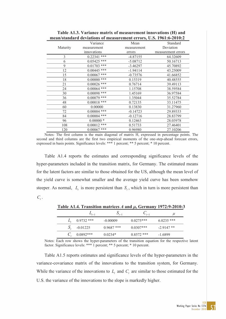
57ECB
Working Paper Series No 1276December 2010
Table A1.3. Variance matrix of measurement innovations (H) and mean/standard deviations of measurement errors, U.S. 1961:6-2010:2
MaturityVariance
measurement innovations
Meanmeasurement errors
Standard Deviation
measurement errors 3 0.22341 *** -4.87155 64.32609 6 0.05425 *** -5.08712 50.16713 9 0.01703 *** -3.46297 45.70892
12 0.00445 *** -1.94114 43.25009 15 0.00067 *** -0.73576 41.66852 18 0.00000 *** 0.15319 40.48555 21 0.00026 *** 0.76714 39.49113 24 0.00064 *** 1.15708 38.59584 30 0.00098 *** 1.45169 36.97584 36 0.00079 *** 1.35044 35.52784 48 0.00018 *** 0.72135 33.11475 60 0.00000 0.13830 31.27960 72 0.00004 *** -0.14723 29.89333 84 0.00004 *** -0.12716 28.83799 96 0.00000 * 0.12463 28.03978 108 0.00012 *** 0.51733 27.46401 120 0.00067 *** 0.96980 27.10206
Notes: The first column is the main diagonal of matrix H, expressed in percentage points. The second and third columns are the first two empirical moments of the one-step-ahead forecast errors, expressed in basis points. Significance levels: *** 1 percent; ** 5 percent; * 10 percent.
Table A1.4 reports the estimates and corresponding significance levels of the
hyper-parameters included in the transition matrix, for Germany. The estimated means
for the latent factors are similar to those obtained for the US, although the mean level of
the yield curve is somewhat smaller and the average yield curve has been somehow
steeper. As normal, tL is more persistent than tS , which in turn is more persistent than
tC .
Table A1.4. Transition matrices A and , Germany 1972:9-2010:3 1tL 1tS 1tC
tL 0.9732 *** -0.00009 0.0275*** 6.0235 ***
tS -0.01225 0.9687 *** 0.0307*** -2.9147 **
tC 0.0892*** 0.0234* 0.8572 *** -1.6899
Notes: Each row shows the hyper-parameters of the transition equation for the respective latent factor. Significance levels: *** 1 percent; ** 5 percent; * 10 percent.
Table A1.5 reports estimates and significance levels of the hyper-parameters in the
variance-covariance matrix of the innovations to the transition system, for Germany.
While the variance of the innovations to tL and tC are similar to those estimated for the
U.S. the variance of the innovations to the slope is markedly higher.
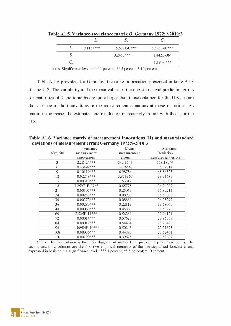
58ECBWorking Paper Series No 1276December 2010
Table A1.5. Variance-covariance matrix Q, Germany 1972:9-2010:3 tL tS tC
tL 0.1167*** 5.872E-07** 6.396E-07***
tS 0.2453*** 1.442E-06*
tC 1.1908 ***
Notes: Significance levels: *** 1 percent; ** 5 percent; * 10 percent.
Table A.1.6 provides, for Germany, the same information presented in table A1.3
for the U.S. The variability and the mean values of the one-step-ahead prediction errors
for maturities of 3 and 6 moths are quite larger than those obtained for the U.S., as are
the variance of the innovations to the measurement equations at those maturities. As
maturities increase, the estimates and results are increasingly in line with those for the
U.S.
Table A1.6. Variance matrix of measurement innovations (H) and mean/standard deviations of measurement errors Germany 1972:9-2010:3
MaturityVariance
measurement innovations
Meanmeasurement errors
Standard Deviation
measurement errors 3 2.28424*** 34.18545 153.18946 6 0.43499*** 14.76647 75.29714 9 0.10119*** 6.98754 48.86525
12 0.02243*** 3.336367 39.91686 15 0.00310*** 1.53812 37.10091 18 3.25971E-09** 0.65775 36.24207 21 0.00107*** 0.25063 35.89211 24 0.00258*** 0.08989 35.59082 30 0.00373*** 0.08881 34.75297 36 0.00289*** 0.22113 33.68060 48 0.00060*** 0.45867 31.59276 60 2.525E-11*** 0.56281 30.04124 72 0.00014*** 0.57621 28.96569 84 0.00012*** 0.54464 28.20496 96 1.46984E-10*** 0.50245 27.71625 108 0.00036*** 0.44897 27.52461 120 0.00190*** 0.39675 27.68607
Notes: The first column is the main diagonal of matrix H, expressed in percentage points. The second and third columns are the first two empirical moments of the one-step-ahead forecast errors, expressed in basis points. Significance levels: *** 1 percent; ** 5 percent; * 10 percent.
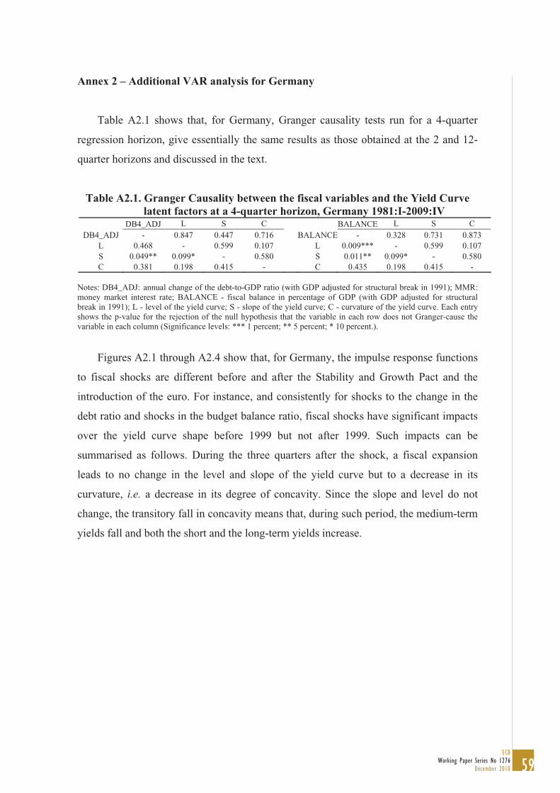
59ECB
Working Paper Series No 1276December 2010
Annex 2 – Additional VAR analysis for Germany
Table A2.1 shows that, for Germany, Granger causality tests run for a 4-quarter
regression horizon, give essentially the same results as those obtained at the 2 and 12-
quarter horizons and discussed in the text.
Table A2.1. Granger Causality between the fiscal variables and the Yield Curve latent factors at a 4-quarter horizon, Germany 1981:I-2009:IV
DB4_ADJ L S C BALANCE L S C DB4_ADJ - 0.847 0.447 0.716 BALANCE - 0.328 0.731 0.873
L 0.468 - 0.599 0.107 L 0.009*** - 0.599 0.107 S 0.049** 0.099* - 0.580 S 0.011** 0.099* - 0.580 C 0.381 0.198 0.415 - C 0.435 0.198 0.415 -
Notes: DB4_ADJ: annual change of the debt-to-GDP ratio (with GDP adjusted for structural break in 1991); MMR: money market interest rate; BALANCE - fiscal balance in percentage of GDP (with GDP adjusted for structural break in 1991); L - level of the yield curve; S - slope of the yield curve; C - curvature of the yield curve. Each entry shows the p-value for the rejection of the null hypothesis that the variable in each row does not Granger-cause the variable in each column (Significance levels: *** 1 percent; ** 5 percent; * 10 percent.).
Figures A2.1 through A2.4 show that, for Germany, the impulse response functions
to fiscal shocks are different before and after the Stability and Growth Pact and the
introduction of the euro. For instance, and consistently for shocks to the change in the
debt ratio and shocks in the budget balance ratio, fiscal shocks have significant impacts
over the yield curve shape before 1999 but not after 1999. Such impacts can be
summarised as follows. During the three quarters after the shock, a fiscal expansion
leads to no change in the level and slope of the yield curve but to a decrease in its
curvature, i.e. a decrease in its degree of concavity. Since the slope and level do not
change, the transitory fall in concavity means that, during such period, the medium-term
yields fall and both the short and the long-term yields increase.
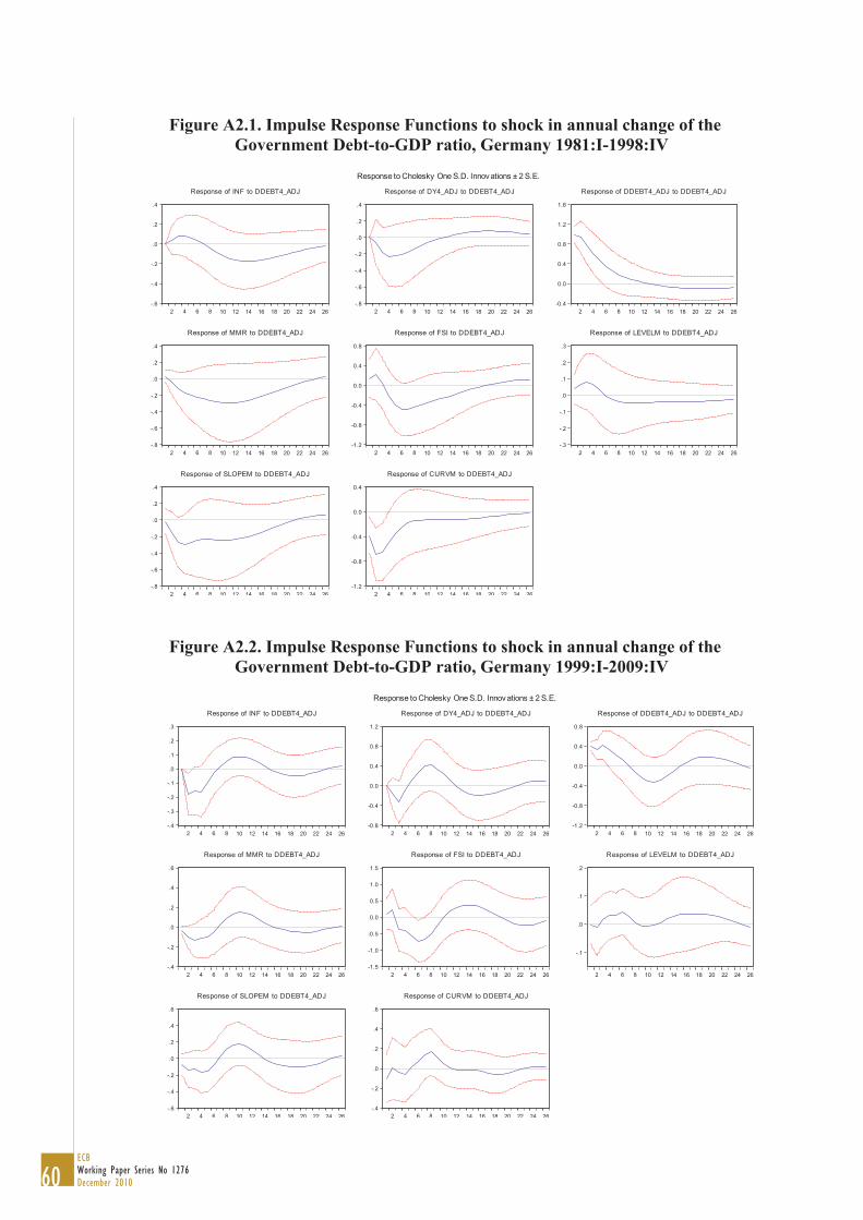
60ECBWorking Paper Series No 1276December 2010
Figure A2.1. Impulse Response Functions to shock in annual change of the Government Debt-to-GDP ratio, Germany 1981:I-1998:IV
-.6
-.4
-.2
.0
.2
.4
2 4 6 8 10 12 14 16 18 20 22 24 26
Response of INF to DDEBT4_ADJ
-.8
-.6
-.4
-.2
.0
.2
.4
2 4 6 8 10 12 14 16 18 20 22 24 26
Response of DY4_ADJ to DDEBT4_ADJ
-0.4
0.0
0.4
0.8
1.2
1.6
2 4 6 8 10 12 14 16 18 20 22 24 26
Response of DDEBT4_ADJ to DDEBT4_ADJ
-.8
-.6
-.4
-.2
.0
.2
.4
2 4 6 8 10 12 14 16 18 20 22 24 26
Response of MMR to DDEBT4_ADJ
-1.2
-0.8
-0.4
0.0
0.4
0.8
2 4 6 8 10 12 14 16 18 20 22 24 26
Response of FSI to DDEBT4_ADJ
-.3
-.2
-.1
.0
.1
.2
.3
2 4 6 8 10 12 14 16 18 20 22 24 26
Response of LEVELM to DDEBT4_ADJ
-.8
-.6
-.4
-.2
.0
.2
.4
2 4 6 8 10 12 14 16 18 20 22 24 26
Response of SLOPEM to DDEBT4_ADJ
-1.2
-0.8
-0.4
0.0
0.4
2 4 6 8 10 12 14 16 18 20 22 24 26
Response of CURVM to DDEBT4_ADJ
Response to Cholesky One S.D. Innovations ± 2 S.E.
Figure A2.2. Impulse Response Functions to shock in annual change of the Government Debt-to-GDP ratio, Germany 1999:I-2009:IV
-.4
-.3
-.2
-.1
.0
.1
.2
.3
2 4 6 8 10 12 14 16 18 20 22 24 26
Response of INF to DDEBT4_ADJ
-0.8
-0.4
0.0
0.4
0.8
1.2
2 4 6 8 10 12 14 16 18 20 22 24 26
Response of DY4_ADJ to DDEBT4_ADJ
-1.2
-0.8
-0.4
0.0
0.4
0.8
2 4 6 8 10 12 14 16 18 20 22 24 26
Response of DDEBT4_ADJ to DDEBT4_ADJ
-.4
-.2
.0
.2
.4
.6
2 4 6 8 10 12 14 16 18 20 22 24 26
Response of MMR to DDEBT4_ADJ
-1.5
-1.0
-0.5
0.0
0.5
1.0
1.5
2 4 6 8 10 12 14 16 18 20 22 24 26
Response of FSI to DDEBT4_ADJ
-.1
.0
.1
.2
2 4 6 8 10 12 14 16 18 20 22 24 26
Response of LEVELM to DDEBT4_ADJ
-.6
-.4
-.2
.0
.2
.4
.6
2 4 6 8 10 12 14 16 18 20 22 24 26
Response of SLOPEM to DDEBT4_ADJ
-.4
-.2
.0
.2
.4
.6
2 4 6 8 10 12 14 16 18 20 22 24 26
Response of CURVM to DDEBT4_ADJ
Response to Cholesky One S.D. Innovations ± 2 S.E.

61ECB
Working Paper Series No 1276December 2010
Figure A2.3. Impulse Response Functions to shock in the Budget Balance, Germany 1981:I-1998:IV
-.4
-.2
.0
.2
.4
2 4 6 8 10 12 14 16 18 20 22 24 26
Response of INF to BALANCE
-.4
-.2
.0
.2
.4
.6
2 4 6 8 10 12 14 16 18 20 22 24 26
Response of DY4_ADJ to BALANCE
-.3
-.2
-.1
.0
.1
.2
.3
.4
2 4 6 8 10 12 14 16 18 20 22 24 26
Response of BALANCE to BALANCE
-.4
-.2
.0
.2
.4
.6
2 4 6 8 10 12 14 16 18 20 22 24 26
Response of MMR to BALANCE
-.8
-.4
.0
.4
.8
2 4 6 8 10 12 14 16 18 20 22 24 26
Response of FSI to BALANCE
-.2
-.1
.0
.1
.2
.3
2 4 6 8 10 12 14 16 18 20 22 24 26
Response of LEVELM to BALANCE
-.6
-.4
-.2
.0
.2
.4
.6
2 4 6 8 10 12 14 16 18 20 22 24 26
Response of SLOPEM to BALANCE
-0.4
0.0
0.4
0.8
1.2
2 4 6 8 10 12 14 16 18 20 22 24 26
Response of CURVM to BALANCE
Response to Cholesky One S.D. Innovations ± 2 S.E.
Figure A2.4. Impulse Response Functions to shock in the Budget Balance, Germany 1999:I-2009:IV
-.2
-.1
.0
.1
.2
.3
.4
2 4 6 8 10 12 14 16 18 20 22 24 26
Response of INF to BALANCE
-1.2
-0.8
-0.4
0.0
0.4
0.8
2 4 6 8 10 12 14 16 18 20 22 24 26
Response of DY4_ADJ to BALANCE
-.4
-.2
.0
.2
.4
.6
2 4 6 8 10 12 14 16 18 20 22 24 26
Response of BALANCE to BALANCE
-.4
-.3
-.2
-.1
.0
.1
.2
.3
2 4 6 8 10 12 14 16 18 20 22 24 26
Response of MMR to BALANCE
-1.0
-0.5
0.0
0.5
1.0
1.5
2 4 6 8 10 12 14 16 18 20 22 24 26
Response of FSI to BALANCE
-.2
-.1
.0
.1
.2
2 4 6 8 10 12 14 16 18 20 22 24 26
Response of LEVELM to BALANCE
-.4
-.2
.0
.2
.4
.6
2 4 6 8 10 12 14 16 18 20 22 24 26
Response of SLOPEM to BALANCE
-.4
-.2
.0
.2
.4
2 4 6 8 10 12 14 16 18 20 22 24 26
Response of CURVM to BALANCE
Response to Cholesky One S.D. Innovations ± 2 S.E.

Work ing PaPer Ser i e Sno 1118 / november 2009
DiScretionary FiScal PolicieS over the cycle
neW eviDence baSeD on the eScb DiSaggregateD aPProach
by Luca Agnello and Jacopo Cimadomo