Fiscal delegation in a monetary union:Instrument assignment and stabilization properties∗

Henrique S. Basso and James CostainBanco de Espana, Calle Alcala 48, 28014 Madrid, Spain

henrique.basso@bde.es, james.costain@bde.es

May 2017

Abstract. Motivated by the failure of fiscal rules to eliminate deficit bias in Eu-rope, this paper analyzes an alternative policy regime in which each member stategovernment delegates at least one fiscal instrument to an independent authority with amandate to avoid excessive debt. Other fiscal decisions remain in the hands of membergovernments, including the allocation of spending across different public goods, andthe composition of taxation. We study the short- and long-run properties of dynamicgames representing different institutional configurations in a monetary union. Dele-gation of budget balance responsibilities to a national or union-wide fiscal authorityimplies large long-run welfare gains due to much lower steady-state debt. The presenceof the fiscal authority also reduces the welfare cost of fluctuations in the demand forpublic spending, in spite of the fact that the authority imposes considerable “austerity”when it responds to fiscal shocks.

Keywords: Fiscal authority, delegation, decentralization, monetary union, sovereigndebtJEL classification: E61, E62, F41, H63

∗Views expressed in this paper are those of the authors, and should not be attributed to theBanco de Espana or the Eurosystem. The authors are grateful for helpful comments from GiancarloCorsetti, Francesco Giavazzi, Jordi Galı, Luisa Lambertini, Eric Leeper, Javier Perez Garcıa, FedericoSignoretti, and Carlos Thomas, as well as seminar participants at the Banco de Espana (including the“Fiscal Sustainability: XXI Century” conference), at UC Santa Cruz, at the Bank of Finland, at theSimposio de Analisis Economico 2016, and at the 19th Banca d’Italia Workshop on Public Finance.The authors take responsibility for any errors.

1

1 Introduction

The legacy of high debt in the aftermath of recent global financial crises leaves policy

makers searching for stronger frameworks to ensure fiscal sustainability, especially in

Europe. In this context, many countries have now established agencies independent

of government with a mandate to monitor fiscal trends and to assess compliance with

fiscal rules. In this paper, we study the effects of a more ambitious form of fiscal

delegation, in which an independent authority is given direct control of one or more

fiscal instruments, with a mandate to ensure long-run budget balance.

That is, we study a regime in which member state governments maintain control

of almost all their fiscal decisions, except for a single instrument, which would instead

be set by an outside agency, independent of the government, with the goal of avoiding

excessive debt accumulation. While this type of fiscal delegation might benefit any

country that suffers from deficit bias, at the present time it may be more politically

realistic in Europe, where core countries worry about ballooning peripheral debt, while

peripheral countries fret about their inability to protect themselves unilaterally against

financial panics and speculative attacks. These concerns highlight the possibility of a

mutually beneficial accord, in which institutions to prevent the propagation of sovereign

and banking risks are made available to any peripheral countries that delegate control

of at least one powerful fiscal instrument to an agency of the European Union, such as

the new European Fiscal Board.1 Compared with existing fiscal rules and the intrusive

monitoring that comes with activation of the Excessive Deficit Procedure, delegating a

fiscal instrument to Brussels could both prove to be a more credible guarantee of fiscal

sustainability from creditors’ point of view, and simultaneously, a less burdensome

constraint on national fiscal sovereignty from debtors’ point of view.

In previous work (Basso and Costain, 2016) we studied how delegation of fiscal

instruments to an independent authority affects long-run, steady-state debt accumula-

tion in a monetary union. We identified several distinct mechanisms through which an

independent fiscal authority would tend to restrain debt growth: first, the debt aver-

sion induced by its mandate; second, its greater patience, compared with the elected

government; and third, the internalization of free-riding problems associated with de-

centralized fiscal choices in a monetary union. We extend this analysis in two crucial

dimensions. First, we investigate whether correcting long-term debt biases hinders the

cyclical stabilization of fluctuations in the demand for public spending. Second, we

relax the (probably unrealistic) assumption that an independent fiscal authority could

1For a description of the European Fiscal Board, see European Commission (19 October 2016).

2

control debt issuance directly, and instead consider dynamic games where the control

variables are public spending and taxes, while debt is determined as a residual.

We carry out our analysis in a reduced-form macroeconomic model in which output

is decreased by taxes and increased by surprise inflation, under the assumption that

society values low inflation, high output, and high public spending. We study how

the equilibrium of the dynamic policy game differs depending on which instruments

are controlled by each of the institutions considered (member state governments, the

central bank of the monetary union, and independent fiscal authorities either at the

national or union-wide level). All policy-making institutions are assumed to be benev-

olent planners, but (as in Rogoff, 1985) we assume that their different mandates lead

them to weight the components of social welfare differently. In particular, we make

two mild assumptions about institutional preferences: (1) elected institutions are more

impatient than nonelected ones, and (2) an institution mandated to achieve a simple,

feasible, quantitative goal will value that goal more strongly than the rest of soci-

ety does. Since institutions differ in their preferences, the irrelevance of instrument

assignment found by Dixit and Lambertini (2003a) does not apply.

Building on a simple macroeconomic model and a simple approach to institutional

preferences has two big advantages. First, it allows us to solve our dynamic game in

a fully nonlinear way, computing the economic dynamics and welfare implications in

steady state and along transition paths and in response to stochastic shocks. In our

numerical simulations, delegation to a fiscal authority implies a large decrease in steady-

state debt, inflation, and tax burdens, and raises social welfare almost to the level

achieved by a committed social planner. On the other hand, one might conjecture that

these long-run gains from fiscal discipline come at the cost of less effective stabilization

policy. However, this is not true: we find instead that establishing a fiscal authority

reduces the welfare cost of fluctuations in the demand for public spending, in spite

of the fact that the authority imposes considerable “austerity” when it responds to

fiscal shocks. We evaluate the cost of fluctuations both from an ex ante perspective

(expected losses due to future variance around the mean path), and also from an ex

post perspective (the welfare loss due to suffering a large negative shock to the fiscal

balance). From either perspective, the welfare cost of fluctuations is smaller in an

economy with a fiscal authority than it is in the status quo monetary union.

A second advantage of our simple setup is that we can focus on the details of the

policy game, in terms of instrument assignment and the timing of moves. Each policy

maker in our framework acts as a discretionary Ramsey planner, and in equilibrium

each planner must anticipate how its own control variables impact debt and thereby

affect the future choices of the other planners. A crucial observation is that the Euler

3

equation(s) determining debt dynamics reflects the impatience of the policy maker(s)

that actually chooses debt. So when we assume that the government or the fiscal

authority controls the debt, that agent’s discount factor enters the formula for the long-

run deficit level. But under the more realistic assumption that the government chooses

public spending, the fiscal authority chooses taxes, and the central bank chooses the

inflation rate, all three of these instruments determine debt jointly, and three Euler

equations reflecting three different discount factors all play a role in the dynamics.

Inflation bias becomes more severe in this scenario, and the fiscal authority becomes less

effective at controlling debt. Nonetheless, our main conclusions about the advantages

of fiscal delegation remain unchanged.

In the remainder of this section, we briefly review the related literature. We then

define the economic environment of our model. In Section 3, we define a series of

policy games representing different institutional configurations; we compute equilibria

of these games and discuss their long-run and short-run implications for debt, inflation,

and social welfare. Section 4 discusses how fiscal delegation might be implemented, in

practice, in the European context. Finally, Section 5 concludes.

1.1 Related literature

Economists from Mundell (1961) to Eichengreen and Wyplosz (1998) and Farhi and

Werning (2015) have emphasized the fiscal challenges implied by losing the freedom to

set monetary policy independently as a consequence of joining a monetary union. The

literature on monetary and fiscal interactions (Leeper, 1991; Sims, 2013) also points to

the fragility of monetary unions: the set of monetary and fiscal rules consistent with

solvency and equilibrium determinacy is likely to be reduced by joining a monetary

union (Bergin, 1998; Sims, 1999; Leith and Wren-Lewis, 2011). Yet another factor

that may increase the fiscal vulnerability of monetary unions is deficit bias. Dixit and

Lambertini (2003b) constructed an example in which joining a monetary union has

no effect on policy outcomes if all policy makers have identical objective functions.

But when policy makers’ preferences differ in plausible ways, for instance due to the

effects of electoral politics (Alesina and Tabellini, 1990; Battaglini, 2011), then joining

a monetary union can increase deficit bias, as multiple authors have shown (Beetsma

and Bovenberg, 1999; Buti, Roeger, and In’t Veld, 2001; Beetsma and Jensen, 2005;

Chari and Kehoe, 2007).

Following the logic of Rogoff (1985), policy delegation may be an effective solu-

tion for the biases that arise when excessively impatient policy makers face incentives

to break past promises. This insight is potentially applicable to deficit bias, as well

4

as inflation bias. Hence, over recent decades, as monetary policy delegation to inde-

pendent central banks has become the norm, many economists have also advocated

delegating some fiscal responsibilities to institutions independent of government. The

literature distinguishes fiscal councils— which monitor but do not implement fiscal

policy actions— from independent fiscal authorities (IFAs), which would actually con-

trol some of the fiscal decisions that are currently in the hands of government.2 Fiscal

councils are by now common, and are mandated under the recent European “Fiscal

Compact” treaty (European Council, 2012), but IFAs remain hypothetical.

Two main classes of IFA have been proposed. On one hand, the IFA might set a

deficit target, at the start of the annual budget cycle, which the government is (some-

how) bound to respect; proposals of this type include von Hagen and Harden (1995);

Eichengreen, Hausmann, and von Hagen (1999); and Wyplosz (2005). Alternatively,

an IFA might exercise executive control over some fiscal instrument with a strong bud-

getary impact; proposals include Ball (1997); Gruen (1997); Seidman and Lewis (2002);

Wren-Lewis (2002); and Costain and de Blas (2012a). These numerous practical pro-

posals contrast with the dearth of theoretical work to model the effects of fiscal policy

delegation. Some authors take the nonexistence of IFAs today as evidence that fiscal

delegation is not feasible, because fiscal decisions are multidimensional, complex, and

inherently political due to their redistributive implications.3 But this argument does

not apply to the fiscal framework considered in our model, for several reasons. First,

we assume that only one instrument (or a small subset of instruments) is delegated.

Second, we consider instruments with an across-the-board budget impact, thus min-

imizing distributional issues. Concretely, we compare delegation of debt issuance to

delegating control of the overall level of taxes. Third, we assume the mandate of the

IFA reflects a largely quantitative goal, such as maintaining long-run solvency, again

minimizing distributional issues.4

Even if fiscal delegation proves effective for reducing deficit bias, it is also important

to ask how it affects the stabilization of shocks, which may require countercyclical

policies and accommodative changes in debt levels. Leith and Wren-Lewis (2011)

look at monetary and fiscal interactions when sovereign debt is present. They find

that stabilization of fiscal shocks is heavily influenced by the effect of inflation on

2See Debrun, Hauner, and Kumar (2009); Hagemann (2010); and Costain and de Blas (2012a) forsurveys of fiscal policy delegation.

3See Hagemann (2010), Sec. II.C; or Calmfors (2011), Sec. 1.

4From a political economy perspective, Alesina and Tabellini (2007), Eggertsson and Borgne (2010),and Maskin (September 29, 2016) discuss the reasons why a democratic society may prefer to delegatecertain types of decisions from politicians to unelected technocrats.

5

the competitiveness of each union member, requiring optimal policy from a country

perspective to change debt gradually. Our reduced form model does not have variations

of terms of trade, which could amplify the shortcomings of fiscal delegation in providing

adequate stabilization. However, as opposed to the framework there, we solve for both

the dynamics and the steady state under discretion and find that the debt biases under

a monetary union are sufficiently strong that any gains from issuing more debt during

the transition are offset, making welfare higher under fiscal delegation. Gnocchi and

Lambertini (2016) also focus on public debt under a distortionary steady state, but

as opposed to us they always retain monetary policy commitment. Leeper, Leith, and

Liu (2016) also stress the importance of non-linear effects incorporated in models of

monetary-fiscal policy interaction solved using global methods. They find that in a

single country model, lack of commitment generates debt stabilization bias, as is the

case in our model. Interestingly, they find that for high levels of debt, monetary policy

is used more heavily; inflation and lower rates are used to reduce debt.

In contrast to the framework we study here, many high-profile calls for Euro-

pean institutional reforms have assumed that achieving adequate protection against

speculative attacks and banking crises makes full political integration inevitable (see

De Grauwe, 2012; Soros, 10 April 2013; or Pisani-Ferry, 2012). We agree that getting

fiscal policy right is crucial for strengthening monetary policy, but we argue that the

necessary reforms are more limited than is commonly supposed. What is essential is

that European authorities must be able to ensure long-run national budget balance,

and for this they must control at least one fiscal instrument of sufficient power in each

member state. In accord with the principle of subsidiarity, all other fiscal decisions

can remain at the national level. Sims (September 20, 2012) likewise stresses that fis-

cal discipline requires European control over some powerful budget instrument in each

member state, arguing that further fiscal integration is neither necessary nor politically

plausible. Similarly, some limited European tax powers form an essential backstop for

banking union, as envisioned by Schoenmaker and Gros (2012) or Obstfeld (2013), but

further fiscal integration is not required under these proposals.

2 The economic environment

Our setup extends the reduced-form framework of Beetsma and Bovenberg (1999) and

Basso and Costain (2016). It is not our goal to explain the imperfections in public

institutions’ decisions, such as excessive impatience or deficit bias, which have been

discussed extensively in the political economy literature. Instead, we aim to model

these features parsimoniously in order to study how equilibrium outcomes differ across

6

games in which policy variables are controlled by different sets of institutions. In

particular, we investigate how systematic policy biases are damped or enhanced by

different institutional configurations, for a typical country in a monetary union. To

address the effects on a typical country (and to simplify the math), we assume all

countries are symmetric.5

Time is discrete. Several regions j ∈ 1, 2, ...J each benefit from local public

spending, and face region-specific budget constraints. These regions might be consid-

ered nations, or subnational areas. Together, they form a monetary union, in which a

single inflation rate applies.

2.1 Social welfare and budget constraints

Let time t private-sector output in country j be xj,t. Our main macroeconomic

assumptions are that inflation πt stimulates output when it is unexpectedly high

(πt > πet ≡ Et−1πt), and that distorting taxes τj,t decrease output relative to its “nat-

ural” level x. That is,

xj,t = x+ ν(πt − πet − τj,t). (1)

Social welfare decreases quadratically as output, inflation, and government services

gj,t deviate from their bliss points. The bliss point for inflation is assumed to be zero,

and that for output is a constant x > 0. The bliss point for public spending, gj,t, varies

stochastically over time:6

gj,t = g + sj,t, (2)

sj,t = ρsj,t−1 + εj,t, (3)

where g > 0 is a constant and εj,t is normal i.i.d. shock with mean zero and variance

σ2. The loss function for region j is7

LSj = E0

T∑t=0

βtSαπSπ

2t + (xj,t − x)2 + αgS (gj,t − gj,t)2 . (4)

The weights απS > 0 and αgS > 0 represent the relative importance of deviations

of inflation and public services from their bliss points; without loss of generality the

weight on output deviations is one. The discount factor for social welfare is βS < 1.

5Small asymmetries between countries leave our results qualitatively unchanged; see footnote 15.

6The bliss points x and gj,t should be interpreted as extremely high levels of private and publicconsumption that are unlikely to be budget-feasible.

7Alesina and Tabellini (1987) derive an output relation of the form (1) from a more completemodel. Leith and Wren-Lewis (2011) derive a social welfare function of the form (4) from a NewKeynesian framework with government spending in the utility function.

7

Since we are modeling a set of independent states that lack consensus for full polit-

ical integration, we assume that policy is constrained by a distinct budget constraint

for each region. We write total government expenditure in region j at time t as qj,tgj,t,

where gj,t represents the quantity of public services, and qj,t is their price (in con-

sumption units). Region j has only two sources of revenue for its spending, both

distortionary: tax revenues τj,t, and seignorage revenues κπt (assumed to be linear in

inflation). Now, let dj,t−1 be the real debt of region j at the end of period t − 1. We

use bars to represent interregional averages; hence dt−1 = 1J

∑Jj=1 dj,t−1 represents real

average debt in the monetary union. We impose the following budget constraint on

region j:

dj,t =[R(dt−1) + χ(πet − πt)

]dj,t−1 + qj,tgj,t − τj,t − κπt. (5)

Here, R(dt−1) represents the expected real interest rate, while R(dt−1) +χ(πet − πt)is the ex post real interest rate, after inflation is realized. This formulation embodies

two key assumptions: nominal debt, and interest rate contagion. Parameter χ ∈ [0, 1]

can be interpreted as the fraction of debt that is nominal, and which therefore loses real

value in response to surprise inflation. Contagion is modeled by making the interest rate

a function of average debt in the union, dt−1, rather than country j’s own debt. Thus,

increased debt of region j raises the interest rate on bonds issued by all union members

(and likewise their debt affects the interest rate facing region j).8 For simplicity, we

assume a linear functional form:

R(dt) = 1 + r0 + δdt =1

βS+ δdt, (6)

which says that savers are willing to hold a “target” debt level d∗ ≡ 0 when the

interest rate just compensates their impatience.9 In addition to (5), debt must respect

an infinite horizon “no-Ponzi” condition, which simply means that expected interest

payments suffice to make it worthwhile for the private sector (with the appropriate

discount rate) to hold the bonds.

8Broto and Perez-Quiros (2013) present empirical evidence on interest rate contagion in Europe.Our formulation oversimplifies contagion; in practice some countries have been “safe havens”, bene-fitting form lower interest rates when the market began to distrust peripheral European debt. Ourinterest rate specification is best seen as representing contagion across peripheral countries. Delegationto a fiscal authority might be less relevant for a safe-haven country; but the presence of a safe-havencountry does not negate our analysis of the role of fiscal delegation for peripheral countries.

9But this is just a normalization. Assuming R(dt) = 1βS

+ δ(dt − d∗), where d∗ is an arbitrarytarget for debt, does not alter the qualitative results. So for simplicity, we set the target to zero.

8

Total public services in region j, gj,t, are a constant-elasticity aggregate of a variety

of differentiated services gj,k,t:

gj,t =

(∫ 1

0

ωj,k,t (gj,k,t)η−1η dk

) ηη−1

. (7)

where η > 1, and ωj,k,t > 0 are i.i.d. weights on the different services k. Total gov-

ernment spending is a sum over all public goods,∫ 1

0gj,k,tdk. Spending is allocated to

minimize the cost of the aggregate public services provided:

qj,tgj,t ≡min

gj,k,t1k=0

∫ 1

0

gj,k,tdk s.t.

(∫ 1

0

ωj,k,t (gj,k,t)η−1η dk

) ηη−1

> gj,t. (8)

Equation (8) serves to define the price of government services, qj,t.

We consider two possible scenarios for the public spending decision. On one hand,

the fiscal policy maker may know the distribution of ωj,k,t, but not observe its realiza-

tion. Then it is optimal to allocate spending equally across all goods, so that

qj,t = qH ≡ (Eω)η

1−η . (9)

At the opposite extreme, the policy maker may observe wj,k,t before choosing gj,k,t. It

is then optimal to spend more on the most-demanded services, according to

gj,k,tgj,l,t

=

(ωj,k,tωj,l,t

)η. (10)

This more efficient allocation makes aggregate public services less expensive:

qj,t = qL = (Eωη)1

1−η < qH . (11)

3 Policy games

3.1 Policy makers’ objectives

Next, we study equilibrium outcomes in scenarios S where several policy institutions

I interact. While all policy makers are essentially benevolent, the weights in their loss

functions LI differ from (4) in accordance with two realistic principles. First, policy

makers subject to democratic election are assumed to be impatient; second, policy

makers subject to a simple, quantitative mandate are assumed to value that goal more

strongly than society at large.

Our status quo monetary union scenario supposes a central bank C that interacts

with many regional governments Gj. The central bank chooses inflation for the whole

9

monetary union. It sums losses symmetrically across all J regions, with weight απC >

απS on inflation, weight αxC ≡ 1 on output, and weight αgC = αgS on public spending.

Each regional government Gj chooses some fiscal variables for region j, and its loss

function LGj only considers terms related to region j. It places weight απG = απS on

inflation, weight αxG ≡ 1 on output, and weight αgG = αgS on public spending.

Our alternative institutional scenarios will include other types of players. One envi-

ronment considered is the replacement of the regional governments by a single federal

government G that controls fiscal variables in all regions j. The federal government’s

loss function includes terms for all regions j, with the same weights as the regional

governments in the status quo scenario: απG = απS, αxG ≡ 1, and αgG = αgS.

We also study economies in which some fiscal instruments are delegated to a debt-

averse fiscal authority. This authority may be established by and for region j, in

which case we will call it Fj, and its loss function will include region j terms only.

Alternatively, it may be a union-wide institution, in which case we will call it F , and

we will assume that it sums losses across all regions. The loss coefficients of Fj and F

are απF = απS on inflation, αxF ≡ 1 on output, αgF = αgS on public spending, and

αdF > 0 on debt. Note that the fiscal authority is the only player that cares specifically

about the debt level, which does not appear in the social welfare function. We will

sometimes use the notation αdC = αdG ≡ 0 to emphasize the fact that the central bank

and the governments do not care specifically about debt.

Hence, while all policy institutions are assumed to value the same goals as society

and the planner, their different roles imply some differences in priorities, reflected in

the weighting coefficients shown in Table 1. The government is more impatient than

society, due to the short time horizons of electoral politics. Since the central bank and

the fiscal authority are insulated from political pressures, they are more patient than

the government. Moreover, since the central bank has a mandate to achieve a target

inflation rate, it dislikes inflation variability more than society does.10 Likewise, we

assume that the fiscal authority has a mandate to stabilize debt around some target

level, so it has a positive debt coefficient.

To obtain an equilibrium with intuitively reasonable properties, we impose a set of

natural restrictions on the quadratic objective functions.11

10Alesina and Tabellini (2007) discuss why society may prefer to delegate tasks with quantifiableobjectives to bureaucrats, instead of leaving them up to the democratic government.

11The role of these restrictions is discussed in depth in Basso and Costain (2016).

10

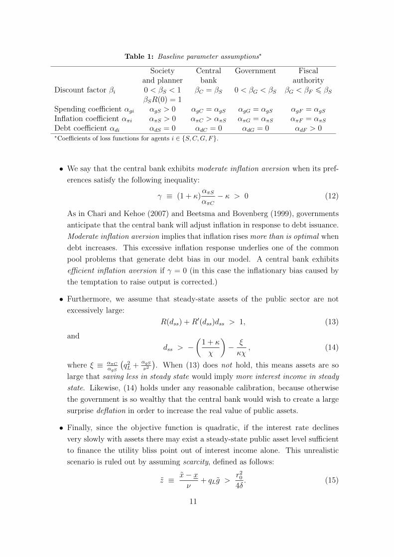
Table 1: Baseline parameter assumptions∗

Society Central Government Fiscaland planner bank authority

Discount factor βi 0 < βS < 1 βC = βS 0 < βG < βS βG < βF 6 βSβSR(0) = 1

Spending coefficient αgi αgS > 0 αgC = αgS αgG = αgS αgF = αgSInflation coefficient απi απS > 0 απC > απS απG = απS απF = απSDebt coefficient αdi αdS = 0 αdC = 0 αdG = 0 αdF > 0∗Coefficients of loss functions for agents i ∈ S,C,G, F.

• We say that the central bank exhibits moderate inflation aversion when its pref-

erences satisfy the following inequality:

γ ≡ (1 + κ)απSαπC− κ > 0 (12)

As in Chari and Kehoe (2007) and Beetsma and Bovenberg (1999), governments

anticipate that the central bank will adjust inflation in response to debt issuance.

Moderate inflation aversion implies that inflation rises more than is optimal when

debt increases. This excessive inflation response underlies one of the common

pool problems that generate debt bias in our model. A central bank exhibits

efficient inflation aversion if γ = 0 (in this case the inflationary bias caused by

the temptation to raise output is corrected.)

• Furthermore, we assume that steady-state assets of the public sector are not

excessively large:

R(dss) +R′(dss)dss > 1, (13)

and

dss > −(

1 + κ

χ

)− ξ

κχ, (14)

where ξ ≡ απCαgS

(q2L +

αgSν2

). When (13) does not hold, this means assets are so

large that saving less in steady state would imply more interest income in steady

state. Likewise, (14) holds under any reasonable calibration, because otherwise

the government is so wealthy that the central bank would wish to create a large

surprise deflation in order to increase the real value of public assets.

• Finally, since the objective function is quadratic, if the interest rate declines

very slowly with assets there may exist a steady-state public asset level sufficient

to finance the utility bliss point out of interest income alone. This unrealistic

scenario is ruled out by assuming scarcity, defined as follows:

z ≡ x− xν

+ qLg >r2

0

4δ. (15)

11

3.2 The generic policy game

To describe policy-makers’ optimization problems in each institutional scenario S, let~dt−1 ≡ dj,t−1Jj=1 be the vector of real debts of all the regions in the monetary union at

the beginning of period t, and similarly let ~st−1 and ~εt be vectors describing the shocks

to the government spending bliss point (its level at t − 1, and the innovation at t).

These three variables obviously affect equilibrium quantities. Pre-existing debt shifts

the current budget constraint; the lagged shock sj,t−1 shifts the expected demand for

public spending at the time expectations πet are formed; and thereafter the innovation

εj,t determines the new level of public demand, gj,t = g+ρsj,t−1+εj,t. Here we will study

equilibria that depend on the set of state variables ~Ωt ≡ (~dt−1, ~st−1,~εt), but no others.

By restricting attention in this paper to equilibria that depend only on the minimal

state ~Ωt, we rule out equilibria with more complex forms of history dependence, such

as reputational effects.

Thus, consider a policy maker Ij who acts in region j only, where I ∈ G,F. The

generic decision problem of such a policy maker can be written as:

V Ij(~Ωt) =max

ΘIjt

−1

2

απIπ

2t +

(xj,t + ν(πt − πet − τj,t)− x

)2+ αgI (gj,t − gj,t)2 + αdId

2j,t

+ βIEtVIj(~Ωt+1) + ΛIj

t

[dj,t −

(R(dt−1

)+ χ(πet − πt)

)dj,t−1 + τj,t + κπt − qj,tgj,t

].

(16)

This problem may represent the decision of a local government Gj or a local fiscal au-

thority Fj. The objective function contains quadratic losses as inflation, output, and

public spending deviate from their bliss points, with preference weights as described

in Table 1. We also allow for a loss term on debt, because we model the fiscal au-

thority’s mandate by assuming that it dislikes debt accumulation (αdF > 0). The set

of instruments controlled by this policy institution at time t is denoted ΘIjt , and the

multiplier on its budget constraint is ΛIjt . The price of public services gj,t differs with

instrument assignment, with qj,t = qL if public spending is allocated across services

by a local decision maker, or qj,t = qH if spending is instead chosen by some central

authority of the monetary union.

Alternatively, we may consider a policy maker I ∈ C,G, F that controls instru-

ments affecting all regions j:

V I(~Ωt) =maxΘIt

−1

2

απIπ2t +

1

J

J∑j=1

(xj,t + ν(πt − πet − τj,t)− x)2

+ αgI (gj,t − gj,t)2 + αdId2j,t

12

+ βIEtVI(~Ωt+1) +

1

J

J∑j=1

ΛIj,t[dj,t −

(R(dt−1

)+ χ(πet − πt)

)dj,t−1 + τj,t + κπt − qj,tgj,t

]. (17)

This institution’s preferences reflect losses in all regions j, and its decision must respect

a separate budget constraint for each region.

Finding a symmetric solution

We will derive Euler equation systems to characterize the policy functions implied

by each institutional scenario S. We restrict attention to symmetric equilibria in which

all regions j face the same parameters and the same initial conditions, and shocks, if

any, affect all regions equally. In a symmetric equilibrium, the state reduces to an

ordered triple of scalars, Ωt ≡ (dt−1, st−1, εt), as there is no longer any variation in

debt or shocks across j.12 Equilibrium under scenario S can then be characterized

by four policy functions: inflation πt = IS(Ωt), gross borrowing dt = BS(Ωt), output

xt = XS(Ωt), and government expenditure gt = GS(Ωt).

For each policy game we solve the functional equations implied by the Euler system,

approximating the policy functions as Chebyshev polynomials, and evaluating expec-

tations using Gauss-Hermite quadrature. Reducing the dimension of the state space by

imposing symmetry makes it much easier to solve these nonlinear functional equations.

Given the policy functions, we can then simulate the dynamics and calculate some

statistics. For example, we can calculate steady-state debt, defined as the fixed point

of the gross borrowing function when shocks are zero:13

dSss = BS(dSss, 0, 0). (18)

Controls versus residuals

We have written policy makers’ problems supposing that all the variables affected

by the choices of player I ∈ Gj, Fj, C,G, F are included in that player’s choice set,

ΘIt . But two cases should be distinguished. If a given variable yt appears only in the

choice set of one particular player I, then this means that I can unilaterally determine

the value of yt. In this case, we will refer to yt as a control variable of player I.

12No bars or j-subscripts are necessary on these variables since in a symmetric situation there is nodistinction between region-specific variables and cross-region averages.

13The fixed point of (18) using the borrowing function BS from our stochastic simulation, denoteddSss, is the “stochastic steady state”, meaning the point to which the dynamics converge conditionalon an arbitrarily long sequence of shocks equal to zero. For some simulations, we compute equilibriumassuming that the shocks ε have zero variance, making the model deterministic; then the fixed point,denoted dSns, is the nonstochastic steady state of the model.

13

But sometimes a variable yt appears in the choice sets ΘIt and ΘI′

t of two distinct

players I and I ′. In particular, the binding budget constraint at each t means that some

variable yt must be determined by the constraint, conditional on the controls chosen

by the players. We will then call yt a residual variable. For example, in some games

studied in section 3.3, inflation is chosen by the central bank, while taxes and debt are

chosen by the government(s); the quantity of public spending is then determined as the

equilibrium outcome of these simultaneous choices subject to the budget constraint.

Hence, in these games, public spending gj,t will be a residual, appearing in the choice

sets of government Gj and the central bank C. In some of the games of section

3.4, inflation is chosen by the central bank, while taxes and spending are chosen by

the government(s); new debt issuance dj,t is then a residual variable determined in

equilibrium by the budget constraint, appearing in the choice sets ΘGjt and ΘC

t . These

differences in instrument assignment turn out to be quantitatively important.

Welfare measures

To compare policy implications across regimes, it is useful to define notation for

the social welfare function. Each region’s welfare depends both on the policy regime,

and on the debts and shocks of all regions in the union; we define overall social welfare

by aggregating across all regions. Therefore, we calculate welfare as

W S(~Ω) = − 1

J

J∑j=1

LSj, (19)

the negative of the sum of the loss functions LSj, evaluated in the equilibrium that

occurs under institutional framework S, when the aggregate state is ~Ω ≡ (~dt−1, ~st−1,~εt).

In a symmetric situation, equilibrium can be simplified by writing it as a function

of the ordered triple Ωt = (dt−1, st−1, εt) rather than the full state variable ~Ω that char-

acterizes an asymmetric situation. We use the subscript ss to represent a stochastic

symmetric steady state. As such when we compare institutional scenarios S, we will

report debt dSss and inflation πSss. While most of our reported results come from stochas-

tic simulations, to calculate business cycle costs we also perform some nonstochastic

simulations, keeping the symmetry assumption. Welfare in the nonstochastic scenarios

is indicated by subscript n. The subscript ns will distinguish non-stochastic steady

states from stochastic steady states (subscripted ss). Hence:

W Sns ≡ W S

n (dSns, 0, 0), (20)

W Sss ≡ W S(dSss, 0, 0). (21)

14

A social planning problem

Before comparing equilibria across policy regimes, we establish a welfare benchmark

for our economy. For relevance in the European context, we consider a Ramsey planner

who maximizes social welfare taking market equilibrium conditions and region-specific

budget constraints as given. Our planner does not represent any existing European

institution, as it has unrealistic advantages in information and decision-making, but it

is useful as a benchmark against which hypothetical institutions can be compared, when

budgets are not aggregated across regions. For this purpose, we consider a planner that

is omniscient, thus it observes ωj,k,t; committed to a state-contingent inflation function;

cooperative, internalizing any externalities across borders; and Paretian, maximizing

welfare while obeying a distinct budget constraint for each region.

Since the planner commits to state-contingent policies that vary with the realization

of ~εt, we write the planner’s value function in terms of variables known at t − 1, as

V P (~dt−1, ~st−1), The ability to commit means that the planner chooses expected inflation

πet , subject to the constraint that this represents a rational expectation.

V P(~dt−1, ~st−1

)=

maxπet ,Θ

Pt

−1

2Et−1

απSπ2t +

1

J

J∑j=1

(xj,t + ν(πt − πet − τj,t)− x)2

+ αgS (gj,t − gj,t)2

+ βSEt−1VP(~dt, ~st

)+

1

J

J∑j=1

ΛPj,t[dj,t −

(R(dt−1

)+ χ(πet − πt)

)dj,t−1 + τj,t + κπt − qLgj,t

]s.t. πet = Et−1πt. (22)

The controls ΘPt = πt, gj,t, τj,t, dj,tJj=1 should be understood as contingent plans

that vary with ~εt, while πet is an expectation computed prior to the realization of ~εt.

The details of the solution to the planner problem are shown in the appendix. By

setting ~εt = 0 for all t, we can find the steady state analytically:

dPss = 0 and πPss =z

κP, (23)

where

zt =1

J

J∑j=1

(xj,t − xj,t

ν+ qLgj,t

), (24)

κP = κ+απSκαgS

(q2L +

αgSν2

). (25)

15

3.3 Policy games with debt as a control variable

We now compare several policy environments in which some decision maker directly

controls debt emission. Since budget constraints must bind at all times, treating debt

as a control implies that some other variable must be determined at each t by the

constraint, as a residual. The games studied here assume that the variable which

adjusts, to ensure the constraint holds, is public spending.

3.3.1 Institutional scenarios

Scenario M: Status quo model of a large monetary union

First, consider a scenario resembling the Eurozone today, with a single central bank

that chooses inflation πt for the whole union, while J governments Gj each choose re-

gional taxes τjt and regional debt djt. Given τjt, djt, and πt, government j spends the

resources it has available, according to budget constraint (5), so public spending gjt is

determined as a residual. Thus, the central bank’s choice set is ΘCt ≡ πt, gj,tJj=1,

and government j’s choice set is ΘGjt ≡ τjt, djt, gj,t. The market’s inflation expecta-

tions πet are set at the end of t − 1, rationally anticipating the outcome of the game

between the bank and the governments, but all policy makers act under discretion.

In each period and region, the marginal cost of tax distortions is set equal to the

marginal benefit of public spending according to a simple linear relation:

νxj,t =αgSqL

gj,t, (26)

where xj,t = xj,t − x and gj,t = gj,t − gj,t and are the deviations of output and public

spending from their bliss points.

Since the central bank cannot commit, it is tempted to choose higher inflation than

that expected by the public. Its resulting tradeoff between inflation and union-wide

mean public spending is

αgSqL

¯gt = − απCπt1 + κ+ χdt−1

≡ −απC πt, (27)

where we again use a bar to represent a cross-region mean, and have defined an adjusted

inflation variable, πt ≡ πt1+κ+χdt−1

.

When solving the planner’s problem (see the appendix) we find that it equates the

marginal cost of inflation to the average marginal benefit of public spending, so thatαgSqL

¯gt = −απSκπt. Thus, as long as αgG = αgS, the government trades off output versus

public spending just as the planner does. But the dynamics of the monetary union

differ from those of the planning problem in several intuitive ways. We see that the

16

central bank tends to choose more inflation than the planner would, especially when

debt is high. On the other hand, if it dislikes inflation more than the public and the

planner do (απC > απS), this will partially offset the inflation bias caused by its lack

of commitment.

Plugging (26) and (27) into the period budget constraint (5), we find that average

debt in the monetary union evolves according to

dt = R(dt−1

)dt−1 + (1 + χdt−1)(πet − πt)− κ(dt−1)πt + zt, (28)

where κ(dt−1) ≡ κ(1 + κ+χdt−1) + απCαgS

(q2L +

αgSν2

). Under the parameter assumptions

of Table 1, if dt−1 ≥ 0 and the central bank exhibits moderate inflation aversion,

then κ(dt−1) < (1 + κ + χdt−1)κP , which says that due to the central bank’s lack of

commitment, the monetary union has more inflation, relative to its level of private

output and public spending, than the planner’s solution does.

Next, consider the Euler equation that governs fiscal policy over time. If country

j is large, its choice of djt will affect the interest rate (both for its own debt and for

other union members); its debt will also influence the choices of other decision makers

at time t+ 1. But we will simplify by focusing on the limit of a large monetary union

(J = ∞) in which each individual country is infinitesimal. In this case, government j

ignores all the spillovers from its debt, and the region-j Euler equation simplifies to14

gj,t = βGR(dt)Etgj,t+1. (29)

When all countries are symmetric, we can use (27) to rewrite the Euler equation in

terms of inflation:15

πt = βGR(dt)Etπt+1. (30)

Note that since government j controls debt, (30) reflects the government’s discount

factor, in contrast with the planner’s solution, where society’s discount factor appears.

Second, since country j’s debt is a negligible part of the debt of the union, government

j simply takes the interest rate as given. This differs from the planner’s solution, in

which an R′ term appears, because the planner realizes that choosing higher debt in all

14The online appendix to Basso and Costain (2016) states the Euler equations for the finite J case,in which each country j is non-negligible, so that the effects of its debt decision on subsequent choicescannot be ignored.

15Again, we drop the bars on variables since there is no distinction between country-specificvariables and cross-sectional averages. Note that if there are instead some asymmetries across re-gions, then (30) only holds approximately. The exact equation is then πt = βS(R(dt))πt+1 −βSR

′(dt)αgSκαπSqL

Covt+1(gk,t+1, dk,t). But the covariance term is negligible when differences betweencountries are small, so all results in this paper are robust to small cross-country differences.

17

regions raises the interest rate (see (79) in the appendix). Both of these effects imply

faster inflation growth in the monetary union than what we observe in the planner’s

solution; since (26) and (27) link inflation to xt and gt, the output and public spending

loss terms also grow more quickly in the monetary union than the planner would wish.

Rapid growth of these distortions represents deficit bias: it means that the economy

suffers relatively small distortions in the near term, but finances the resulting deficit by

accumulating debt, which must be paid off in the future by suffering larger distortions

in the long run.

Illustrating our solution methodology, the symmetric solution of this scenario can

then be characterized by policy functions BM(Ωt), IM(Ωt), and IM(Ωt) = IM (Ωt)

1+κ+χdt−1

such that the following equations hold:

BM(Ωt) =R (dt−1) dt−1 + (1 + χdt−1)(Et−1[IM(Ωt)]− IM(Ωt))− κIM(Ωt) + zt, (31)

IM(Ωt) = βG(β−1S + δBM(Ωt)

)EtI

M(BM(Ωt), st, εt+1). (32)

where zt ≡ ν−1(x−x)+qLgt. Government spending and output can then be calculated

fromαgSqLGM(Ωt) = −απC IM(Ωt) and νXM(Ωt) =

αgSqLGM(Ωt).

Scenario I: A single country with its own monetary policy

The deficit bias suffered by a monetary union can also be seen by comparing it to

the case of a single country with its own independent central bank. The instrument

assignment is identical to the monetary union environment (ΘCt ≡ πt, gt, ΘG

t ≡τt, dt, gt) but we focus on the case J = 1, instead of the opposite extreme J =∞.

The tradeoffs between output, public spending, and inflation are unchanged, so (26)

and (27) still apply. Therefore the equation governing per capita debt is the same as

in the monetary union:

dt = R (dt−1) dt−1 + (1 + χdt−1)(πet − πt)− κ(dt−1)πt + zt. (33)

The differences show up in the Euler equation, which becomes16

πt = βGEt

(R(dt) +R′(dt)dt +

(γ + χ

απGαπC

dt

)∂πt+1

∂dt

)πt+1. (34)

The parameter γ, defined in (12), indexes the strength of the central bank’s preference

for surprise inflation.

As in scenario M , the discount factor in the Euler equation is βG, reflecting govern-

ment impatience, which raises inflation growth. But other terms in the Euler equation

16To solve equations (33)-(34), we can rewrite them in terms of d and π only, using the fact thatπ(d) = (1 + κ+ χd)π(d) to substitute out π′(d) = (1 + κ+ χd)π′(d) + χπ(d).

18

slow down inflation growth, relative to a monetary union. The government of a single

country recognizes that its debt affects the interest rate it pays, so the term R′(dt)dt

appears in the Euler equation, which reduces inflation growth whenever dt > 0. Sec-

ond, the central bank has an incentive to create surprise inflation (i) to boost output

and (ii) to decrease the real cost of servicing nominal debt; the strength of these in-

centives goes through the parameters γ and χ, respectively.17 Given the bank’s lack

of commitment, the government of a single country knows that its debt will influence

central bank inflation, and hence it cuts its deficit to correct for these inflation bias

terms. Again, this reduces inflation growth, compared with scenario M , where each

government regards the impact of its own debt as negligible.

Scenario G: A federal government for a monetary union

Creating a single government for the monetary union makes its political structure

formally identical to a single country, so our analysis of the J = 1 case applies. There-

fore, as we argued above, two forms of deficit bias should disappear when a monetary

union adopts a single government. Like a single country, but unlike a small member

of a monetary union, a federal government internalizes the effect of its debt on the

interest rate it pays. This gives it an incentive to accumulate less debt than member

states of a monetary union do. Similarly, the federal government recognizes the fact

that the central bank will raise inflation in response to any rise in the average debt

level, whereas small member states in a monetary union would fail to internalize this

effect and would therefore choose more debt on average.

However, in the European context, this setup has a major disadvantage. It gives up

“subsidiarity”: spending decisions are taken at the union level, where less information

is available. This raises the price of public services to qH > qL, more expensive than

they would be if they were allocated locally. The conditions linking inflation, public

spending, and output would then be

¯gt = −απCqHαgS

πt, (35)

¯xt = −απCνπt. (36)

Comparing with the corresponding relations for the monetary union, (26) and (27),

(35)-(36) show that the relation between inflation and output is unchanged, but that

for any given level of inflation and debt, the distance of government services from their

bliss point is increased.

17Under the parameter assumptions of Sec. 3.1, including moderate inflation aversion, we have0 < γ < 1. It can also be shown, under weak assumptions, that ∂π

∂d > 0. Therefore these additionalterms in the Euler equation reduce inflation growth.

19

Summarizing, the dynamics of the symmetric case are analogous to (33)-(34), except

that they now refer to per capita debt in the whole union.

dt = R (dt−1) dt−1 + (1 + χdt−1)(πet − πt)− κG(dt−1)πt + zGt , (37)

πt = βGEt

(R(dt) +R′(dt)dt +

(γ + χ

απGαπC

dt

)∂πt+1

∂dt

)πt+1, (38)

The only difference from scenario I is that public services are more expensive, which

alters the parameters in the equations as follows:

κG(dt−1) ≡ κ(1 + κ+ χdt−1) +απCαgS

(q2H +

αgGν2

), (39)

zGt ≡ ν−1(x− x) + qH gt. (40)

Scenario Fj: Delegation to regional fiscal authorities

While a federal government would avoid some aspects of the deficit bias that plagues

a monetary union, establishing such a government seems a very distant prospect in Eu-

rope today. Just to mention a few of the most critical problems involved, setting up

a central or federal government for Europe would require (1) convincing local politi-

cians to give up power in favor of new central institutions; (2) harmonizing local laws

and constitutions sufficiently to permit European governance; and (3) finding ways to

efficiently address local decisions via central or federal institutions. Even if these chal-

lenges could be overcome (slowly) from a technical perspective, establishing legitimacy

of new European institutions would remain (insurmountably?) difficult, all the more

so as nationalism has grown with recent crises.

This motivates us to ask instead whether delegation of fiscal instruments might serve

as a shortcut to credible long-run debt sustainability, avoiding many of the dilemmas

listed above. Delegating just one (or a few) effectively-designed fiscal instruments might

have a very large impact on budget balance, but would involve less surrender of power

by local politicians than the establishment of a federal government. Relatively fewer

changes to laws and constitutions would be required, and most local fiscal decisions

would remain under local control. Therefore, we now analyze the macroeconomic

implications of some policy games involving delegated fiscal powers.

First, we consider region-specific delegation. Concretely, we consider policy games

in which the central bank chooses inflation for the union, and regional governments

choose taxes and allocate public spending, but the choice of how much debt to issue is

delegated to an independent regional fiscal authority Fj. The overall quantity of local

public spending is treated as a residual variable; thus the instrument assignments are

given by ΘCt ≡ πt, gj,tJj=1, Θ

Gjt ≡ τjt, gj,t, and Θ

Fjt ≡ djt, gj,t. That is to say,

20

the amount of money spent by government Gj is only partly under its control (through

its choice of taxes), but the allocation of these funds across different uses is left entirely

in its hands.

As in scenario M , analysis is greatly simplified by considering a symmetric equilib-

rium with many small countries. Formally, assuming all countries are symmetric and

J = ∞ implies that each country is infinitesimal, so it ignores the impact of its own

debt on interest rates, inflation, and other countries’ debt. Then the Euler equation is

gj,t +qLαdFαgF

dj,t = βFR(dt)Etgj,t+1. (41)

Assuming a symmetric equilibrium, we can then rewrite the dynamics in terms of

inflation and average debt:

dt = R (dt−1) dt−1 + (1 + χdt−1)(πet − πt)− κ(dt−1)πt + zt (42)

πt =αdFαπC

dt + βFR(dt)Etπt+1. (43)

Comparing (28)-(30), the equilibrium system for scenario M , with (42)-(43), we see

two effects of the fiscal authority that inhibit inflation growth. First, for a given dt,

inflation grows more slowly in the presence of the fiscal authority if the government is

less patient than the fiscal authority (βG < βF ). Second, inflation grows more slowly

in the presence of the fiscal authority whenever dt > 0, as long as the fiscal authority

dislikes debt (αdF > 0).

Scenario F: Delegation to a union-wide fiscal authority

Rather than delegating debt issuance to a fiscal authority Fj within each region,

a possibly better alternative might be to delegate the issuance of each country’s debt

to a single authority F established for the union as a whole. Such an authority would

have an incentive to take externalities across regions into account. In this case, the

symmetric dynamics are given by

dt = R(dt−1)dt−1 + (1 + χdt−1)(πet − πt)− κ(dt−1)πt + zt, (44)

πt =αdFαπC

dt + βFEt

(R(dt) +R′(dt)dt +

(γ + χ

απGαπC

dt

)∂πt+1

∂dt

)πt+1. (45)

These equations are simplified using the parameter assumptions in Table 1.

This system combines two properties we have seen before. Like a model with fiscal

authorities at the regional level, debt slows down inflation growth, as long as the fiscal

authority is debt averse (αdF > 0). But in addition, inflation growth is affected by the

impact of debt on the interest rate (R′) and on inflation (∂πt+1

∂dt), because the union-

wide fiscal authority knows it can alter aggregate debt, just as the government did in

scenario I. Since inflation responds positively to a rise in debt, and the central bank

is assumed to exhibits moderate inflation aversion (implying γ > 0), inflation growth

is further reduced in this scenario, compared with scenario Fj.

21

3.3.2 Results

Parameters

We choose parameters so that our quantitative results can be given a plausible

economic interpretation, in spite of the reduced-form nature of our model. Specifically,

we calibrate with reference to the nonstochastic steady state of the baseline monetary

union scenario, taking care to respect the restrictions stated in Section 3.1.

The time unit is a year, and the goods unit is normalized so that annual private

output xMns is one in the nonstochastic steady state of scenario M . We set the discount

rate to βS = 1.02−1, and set δ = 0.03, so that the annual real interest rate is 2% when

debt is zero and 5% when debt is one (100% of output). Since European debt levels

still appear to have a strong tendency to increase, we assume that steady state debt

in scenario M is substantially higher, at dMns = 2. This is consistent with βG = 1.08−1.

We set the fiscal authority’s discount rate halfway between those of the planner and

the government: βF = (βS + βG)/2. We assume that half of debt is nominal, χ = 0.5.

We set ν = 1, implying that if tax collection rises by 1% of private output, then

private output falls by 1%. This is a conservative estimate of tax distortions; Gunter,

Riera-Crichton, Vegh, and Vuletin (2016) estimate that the long-run multiplier of tax

revenue on output is twice as large. Steady state taxes must be mutually consistent

with steady state output; assuming steady-state taxes are τMns = 0.5, we must have

x = xMns+ντMns = 1.5. We assume that inflation will rise to 10% (πMns = 0.1) in the steady

state of the monetary union,18 and that κ = 0.2, meaning that each percentage point of

inflation generates revenues equal to 0.2% of output. Given our assumptions so far, if

locally-produced public goods cost the same as private goods, then steady-state public

services in the monetary union are gMns = 1qL

(τMns + κπMns − r0d

Mns − δ(dMns)2

)= 0.36. We

assume that centralized provision of public goods is 50% more costly, qH = 1.5.

The bliss points x and g are hard to infer from steady-state behavior alone. We

set both to a level far above actual output, x = g = 5, and we confirm through

robustness calculations that large changes in these bliss points (x = g = 3 or 10) leave

our results qualitatively unchanged (see Table 4 for robustness calculations.) Given our

calibration targets and parameters thus far, the first-order condition between public

and private output requires αgS = νqL(xMns − x)/(gMns − g) = 0.8621. Likewise, the

first-order condition between output and inflation requires απC = −|xMns − x|(1 + κ +

χdMns)/πMns = 88. We calibrate the social cost of inflation so that the planner’s solution

22

Figure 1: Borrowing and inflation policies. Comparing institutional scenarios

Notes: Comparing policy functions across institutional scenarios, assuming debt is a control variable.

Left: Gross borrowing: debt dt as a function of dt−1.

Right: Inflation πt as a function of dt−1.

Black: planner. Blue: monetary union. Green: one country. Magenta: regional FAs. Red: Union-wide

FA. Cyan: federal government. Red stars: steady states.

has 2% inflation in steady state, which implies απS = 39.3333. Finally, we set the fiscal

authority’s loss coefficient on deviations of debt from target to αdF = 0.5.

Policy functions

We characterize the behavior of each scenario S by calculating the nonlinear policy

functions dt = BS(Ωt) and πt = IS(Ωt) consistent with the Euler equations derived

from that scenario. In this subsection we report the results for two specifications, both

of which are stochastic: an i.i.d. and an autocorrelated version. In the simulations, the

public spending demand shock εt affects all regions j symmetrically and is assumed

to have mean zero, standard deviation 0.02. For the autocorrelated version, we set

18Note that we have abstracted from default. Hence, steady-state inflation is a stand-in for themany costs associated with excessive debt, which is why we choose a rather high calibration targetfor πMns.

23

ρ = 0.7, so shocks to the spending bliss point die out fairly slowly.19

Figure 1 shows the policy functions under the i.i.d. specification, for scenarios P

(black), M (blue), I (green), Fj (magenta), F (red), and G (cyan). The right-hand

panel shows that the planner chooses nonzero inflation (πPss = 0.02) in the steady

state (dPss = 0). Lacking any nondistortionary revenue source, the planner collects a

small amount of seignorage, increasing very slightly with debt, to optimally trade off

the marginal losses from inflation and from distortionary taxes. In the left panel, the

borrowing function dt = BP (dt−1, 0, 0) has a slope of roughly 0.5. That is, when the

current debt level is one percentage point higher, the planner pays off half within one

period and carries the other half over to the next period.

Relative to the planner’s policies (black), the green curves that represent the equi-

librium policies of a single country (scenario I) are shifted upwards. The inflation

function II is both higher and steeper than the planner’s policy IP , because monetary

policy in scenario I is a discretionary decision, and the temptation to create surprise

inflation becomes stronger as debt increases. The borrowing function BI lies above the

planner’s policy BP because the impatience of the democratic government in scenario

I leads to more borrowing. In steady state, debt in scenario I rises to dIss = 71.5% of

output, with an inflation rate of 7% (see Table 2 for the numbers.)

The policy biases affecting scenario I are reinforced by free-riding effects in the sta-

tus quo monetary union scenario M (blue). The borrowing policy BM lies everywhere

above BI , because governments in scenario M ignore how their debt affects the interest

rate and the incentives of the central bank. Steady-state debt rises to dMss = 199.9% of

output. On the other hand, the inflation policy IM lies slightly below II , because the

central bank recognizes that government incentives are worse in the monetary union

than in a single country, so it restrains inflation at any given debt level. Nonetheless,

since steady-state debt is so much higher in the monetary union, steady-state inflation

also rises in scenario M , to πMss = 10.0%.

In contrast, establishing a fiscal authority shifts the borrowing function down. The

borrowing function of scenario Fj lies below that of scenario M , both because the

regional fiscal authorities are more patient than regional governments, and because the

fiscal authorities are averse to debt. Steady-state debt therefore falls to dFjss = 0.179.20

Also, the borrowing function BFj is less steeply sloped than BM (slope 0.3 rather than

19For comparison when we calculate the costs of business cycles, we will also calculate a fullynonstochastic specification. The nonstochastic case can be computed by assuming that εt has meanand variance equal zero, or by dropping εt entirely from the model so that the policy functions dependon debt only. We have run the calculations both ways, and obtained virtually identical results.

20The fact that BFj lies below BI is calibration-specific; it is not a general result.

24

Table 2: Debt, inflation, and welfare in scenarios S where debt is a control variable∗

Transition Crisis cost,b,c

Debta Inflation Welfareb gainb Crisis costb,c fixing debt Cyclical costb,d

dSss πSss W Sss −WM

ss WS(dMss ,0,0)−WMss WS(dSss,0,ε

g0)−WS

ss WS(0,0,εg0)−WS(0,0,0) WSss−WS

n (dSss,0,0)

Temporary shocks (autocorrelation 0)

Scenario P: Planner

0.1% 2.0% +19.5% +14.9% −0.39% −0.39% −0.12%Scenario I: single country with independent central bank

71.5% 7.0% +15.2% +12.0% −0.41% −0.39% −0.12%Scenario M: status quo monetary union

199.9% 10.0% 0% 0% −0.48% −0.42% −0.13%Scenario Fj: Monetary union with regional fiscal authorities

17.9% 5.8% +18.3% +13.9% −0.39% −0.39% −0.13%Scenario F: Monetary union with union-wide fiscal authority

8.7% 5.6% +18.6% +14.1% −0.39% −0.39% −0.13%Scenario G: Monetary union with union-wide federal government

78.4% 5.5% +14.9% +12.6% −0.47% −0.45% −0.17%aDebt expressed as a fraction of steady state private output of baseline scenario M .bAll welfare changes stated as equivalent variations of private output, starting from nonstochastic steady state of baseline scenario M .c“Crisis” refers to a four-percent rise in public goods demand at time 0, εg0 = 0.02.dComparing stochastic economy with εgt ∼ N(0, 0.02) to nonstochastic economy (εgt ≡ 0).

25

Table 3: Debt, inflation, and welfare in scenarios S where debt is a control variable∗

Transition Crisis cost,b,c

Debta Inflation Welfareb gainb Crisis costb,c fixing debt Cyclical costb,d

dSss πSss W Sss −WM

ss WS(dMss ,0,0)−WMss WS(dSss,0,ε

g0)−WS

ss WS(0,0,εg0)−WS(0,0,0) WSss−WS

n (dSss,0,0)

Correlated shocks (autocorrelation 0.7)

Scenario P: Planner

0.1% 2.0% +19.4% +14.8% −0.75% −0.75% −0.86%Scenario I: single country with independent central bank

71.4% 7.0% +15.3% +12.2% −0.78% −0.75% −0.68%Scenario M: status quo monetary union

199.7% 10.0% 0% 0% −0.90% −0.82% −0.83%Scenario Fj: Monetary union with regional fiscal authorities

17.9% 5.8% +18.4% +14.1% −0.75% −0.74% −0.70%Scenario F: Monetary union with union-wide fiscal authority

8.7% 5.6% +18.7% +14.2% −0.75% −0.75% −0.71%Scenario G: Monetary union with union-wide federal government

78.3% 5.5% 14.8% +12.6% −0.90% −0.88% −0.95%aDebt expressed as a fraction of steady state private output of baseline scenario M .bAll welfare changes stated as equivalent variations of private output, starting from nonstochastic steady state of baseline scenario M .c“Crisis” refers to a four-percent rise in public goods demand at time 0, εg0 = 0.02.dComparing stochastic economy with εgt ∼ N(0, 0.02) to nonstochastic economy (εgt ≡ 0).

26

0.5). This is a sign of austerity: when debt increases for any reason, it converges back

to its steady state more quickly in the economy with a fiscal authority than it does

in the status quo monetary union. Moreover, although the inflation policy IFj lies

(slightly) above II and IM , the lower steady state debt in scenario Fj also reduces

steady-state inflation, to πFjss = 0.058.

Finally, scenario F combines the debt-reducing incentives of scenarios I and Fj.

Like the regional fiscal authorities, a union-wide fiscal authority is less impatient than

national governments, and dislikes debt accumulation (the weights on per capita debt

in the loss functions in scenarios F and Fj are assumed equal). Like the government

of a single country, the union-wide fiscal authority internalizes the impact of its debt

on the interest rate and on central bank behavior (the effects of per capita debt on the

interest rate and on central bank preferences are assumed equal in scenarios F and I).

Therefore the borrowing function in scenario F lies below curves BI and BFj, which

both lie below BM . The resulting steady state debt level is dFss = 0.056, slightly below

that in scenario Fj.21

Interpreting the effects on debt

The steady-state debt ranking depicted in Figure 1 can be understood by consider-

ing the underlying biases that operate in each institutional scenario. The social planner

sets dPss = 0, the optimal steady-state debt. A decentralized economy where all institu-

tions have the same preferences, and where the time inconsistency problem is offset to

the appropriate degree that eliminates inflation bias, would also achieve this optimal

level of debt. In our set-up these conditions are represented by the parameterization

βG = βS and γ = 0.22 However, under the more realistic assumption that democrati-

cally elected officials act as if they are less patient than society as a whole, a positive

bias pushes up steady state debt. In a single country economy, this increase in debt

levels due to impatience is curtailed because the government is aware that (i) higher

debt worsens inflation bias in equilibrium, since it makes the central bank more willing

to raise inflation to boost output and inflate away nominal debt, and (ii) high levels

of debt increase real interest rates (see Beetsma and Bovenberg, 1999, and Leith and

Wren-Lewis, 2013, for discussion of these debt attenuation motives).

21As we discussed in Basso and Costain (2016), steady state debt in scenario Fj can be provedhigher than steady state debt in the planner’s solution, and steady state debt in scenario F is lowerthan that in scenario Fj. But the ranking of debt between scenarios P and F is ambiguous: a union-wide fiscal authority may actually choose a steady-state debt level that is inefficiently low comparedwith the social planner.

22See Dixit and Lambertini (2003a), Chari and Kehoe (2008), and Basso and Costain (2016), Section4.3.2, for in-depth discussion of these points.

27

While the members of a monetary union would benefit, in principle, from cooper-

atively restraining debt for the reasons just mentioned, in equilibrium each member

has an incentive to free-ride, increasing spending and reducing taxes, leaving debt con-

trol to the others. This represents a classic common pool problem, in which the only

equilibrium is that members accumulate too much debt because they fail to internalize

the effects on interest rates and inflation. Regional fiscal delegation, by shifting con-

trol of debt to an institution that is more impatient and less debt tolerant, provides a

countervailing force that limits the biases caused by democratic and non-cooperative

decision processes. Union-wide fiscal delegation has the same effects, but in addition

internalizes the impact of each member’s debt on equilibrium, directly taking account

of the tragedy of the commons.

Welfare implications

Besides lowering debt and inflation, Tables 2-3 also show that delegation to a fiscal

authority implies a large improvement in social welfare (see the third columns of the

tables). The steady-state social welfare W Sss of scenario S is reported as an equivalent

variation in private sector output x, compared with scenario M (hence the welfare

level in scenario M is shown as zero, by construction). The planner’s solution has

the highest steady-state welfare, representing a 19.5% permanent increase in private

sector output, relative to scenario M . This welfare gain both reflects the fact that it is

calculated at the lowest steady-state debt in the table, and the fact that, by definition,

it is the policy that optimizes social welfare at any given debt level. We have also seen

that the scenarios with higher steady-state debt have higher steady-state inflation.

In scenarios M , I, Fj, and F , inflation is related to public and private spending by

(26) and (27), linking higher inflation with larger gaps of public and private spending

from their bliss points. Therefore the ranking of social welfare across these scenarios

is the opposite of their debt ranking: WMss < W I

ss < W Fjss < W F

ss. Crucially, the fiscal

delegation scenarios lie substantially closer to the planner’s welfare level than to that

of the monetary union.

Of course, these welfare comparisons only apply in steady state; switching to a new

institutional regime does not produce welfare gains as large as those seen in the third

column of the tables immediately. Instead, for an economy that starts with a large

stock of debt, delegating fiscal responsibilities (or implementing the planner’s solution)

initially implies a costly transition period in which existing debt is paid off. To take

the costs of this initial austerity into account, the fourth columns of Tables 2 and 3

report the gains of moving to each possible alternative scenario S, starting from the

steady state debt level of scenario M . That is, we compare the welfare each alternative

28

S evaluated at the debt level inherited from the monetary union, W S(dMss , 0, 0), with

the welfare WMss ≡ WM(dMss , 0, 0) of remaining in scenario M .

Even taking into account transition costs, the benefits of delegating instruments

to a fiscal authority are very large, roughly equivalent to a 14% permanent increase

in private sector output, relative to the monetary union. This represents most of the

potential welfare gain from moving to the planner’s solution, which (including transi-

tion costs) is equivalent to a 15% output increase, relative to scenario M . Subtracting

the numbers in the third and fourth columns of Tables 2-3, we see that the initial

austerity cost of fiscal delegation is also large (roughly 4% of output), but the gains

from delegation are sufficient to overwhelm these costs.

Considering that we are solving a reduced-form model, these welfare numbers should

be taken as a qualitative illustration of the effects of fiscal delegation, rather than a

precise quantitative assessment of those effects. Nonetheless, finding welfare gains that

are orders of magnitude larger than Lucas’ (1987) estimate of the cost of business cy-

cles is unsurprising, because interest payments on sovereign debt (owned by foreigners)

are subtracted off of national income, directly affecting the budget available for con-

sumption. Hence, the welfare difference between scenarios M and S, when expressed

as an equivalent output variation, is at least as large as the steady-state change in the

sovereign interest burden, r(dMss )dMss − r(dSss)dSss. Moreover, besides the reduction in

the sovereign interest burden, moving from scenario M to any of the other scenarios

considered here also implies a large decrease in tax distortions and inflation.

Impulse responses

The results thus far suggest that fiscal delegation improves welfare by reducing

long-run debt. But debt accumulation offers a smoothing mechanism that may im-

prove welfare in response to shocks; so it is important to ask whether fiscal delegation

eliminates or weakens a buffer that protects the economy against excessive fluctuation

of payoff-relevant variables. To this end, Figures 2 and 3 compare impulse responses

to shocks to the demand for public spending across scenarios P (black with squares),

M (blue with stars), I (green with “x”), Fj (magenta with diamonds), F (red with

dots), and G (cyan line). We think of an increase in the demand for public spending as

a reasonable stand-in for recent crises in Europe and other advanced economies, where

large amounts of state funds were used to recapitalize banking systems, in an effort to

avoid a major contraction of credit supply to the private sector.

Concretely, the figures suppose a 4% increase in gj,t (from 5 to 5.2) at time 2

(the initial steady state position is shown at time 1, for reference).23 In Fig. 2, the

23This is a big shock. Since the bliss point g is far above equilibrium public spending, fully accomo-dating this demand shock (raising spending by 0.2) would require much more than a 4% percentageincrease in public spending.

29

Figure 2: Temporary public demand shock. Comparing institutional scenarios.

Notes: Impulse responses of debt, inflation, government spending, output, and instantaneous and

cumulated utility to a temporary 4% increase in the public spending bliss point g, assuming debt is a

control variable.

shock is assumed to be uncorrelated over time (as in Table 2), while in Fig. 3, it has

autocorrelation ρ = 0.7. We report the impulse responses as deviations from steady

state (rather than log deviations) so that the absolute size of each response can be

visually compared across scenarios S.

In the planner’s solution of the uncorrelated specification (black in Fig. 2), gov-

ernment spending rises from approximately 0.36 to 0.40 at the time of the shock. To

finance this increase, debt rises from d1 = dPss = 0 to d2 = 0.03, postponing almost

three quarters of the financing to the future. Therefore, there is a persistent decrease

in public spending for t ≥ 3, and a persistent decrease in output at times t ≥ 2, re-

flecting increased taxes. Also, the planner imposes a small burst of surprise inflation

on impact, raising the inflation rate temporarily from 2% to 2.04%. Since output and

public spending both fall relative to their bliss points, and inflation rises, the flow of

30

utility falls on impact by 0.7 utils.24

Turning next to scenario M , the public demand shock is again accommodated,

to roughly the same extent that it was in the planner’s solution. But the monetary

union relies less on increased taxation, so the fall in output is slightly smaller (by

0.011) than it is in the planner’s problem (where output falls by 0.014 on impact).

Instead, the monetary union issues slightly more debt than the planner does (it runs

a deficit of 0.034, raising the debt stock from dMss = 1.999 to d = 2.033 on impact).

More importantly, debt is much more persistent in scenario M than it is in scenario

P , so the shock has greater medium-term effects. Unlike the planner’s solution, where

inflation rises only on impact (when it is unexpected), inflation in the monetary union

responds strongly to increased debt, so there is a persistent rise in inflation and fall in

utility. The last two panels of the graph show the utility loss– the fifth panel shows

the deviation in utility from its steady state level, and the sixth cumulates this utility

loss over time. While the utility loss is smaller on impact in scenario M than it is in

scenario P , the ranking is reversed in the following period; the persistent losses in the

monetary union eventually cumulate to a total utility loss of roughly 0.9 utils, while in

the planner’s solution the cumulated losses are only 0.8.

Thus, scenariosM and P both permit a substantial rise in public spending, and both

delay most of the financing to the future, but the deficit bias in scenario M makes the

costs much more persistent. If we now compare what happens in the fiscal delegation

scenarios (magenta and red lines), we see that the response is less accomodative; public

spending rises by approximately 0.035 rather than 0.04 on impact. Also, there is less

smoothing over time; the rise in debt is around one-third smaller than it is in scenarios

M and P . Hence, more of the fiscal impact must be absorbed on impact by raising

taxes, so the fall in private sector output is much larger (it decreases by 0.18 under

fiscal delegation, rather than 0.11 in scenario M). Hence, instantaneous utility falls

more on impact under fiscal delegation than it does in the other scenarios considered;

but the advantage of this austerity is that debt becomes much less persistent. Just one

period after the shock, output and instantaneous utility are already higher in scenarios

Fj and F than they are in scenarios M and P . And when we sum the utility impact

of the shock over time, the overall loss in the fiscal delegation scenarios is virtually

indistinguishable from that in the planner’s solution, but is somewhat less than the

cumulated loss in the monetary union. In other words, while the fiscal authorities

impose painful austerity on impact, this is compensated by a rapid recovery of utility,

so in intertemporal terms they perform almost as well as the social planner.

24The figures illustrate the welfare impact as measured in utils. For welfare measures expressed asequivalent output variations, see the fifth columns of Tables 2-3.

31

These welfare conclusions are restated numerically in Table 2. The fifth column

reports the welfare impact of a four percent rise in public spending demand, starting

from steady state, in each scenario. That is, it reports W S(dSss, 0, εg0)−W S(dSss, 0, 0) for

each scenario S, where εg0 = 0.02, which is the present discounted value of the utility

losses caused by the shock graphed in Fig. 2. Unsurprisingly, the intertemporal welfare

loss is smallest in the social planner’s solution. But strikingly, even though output

falls more sharply on impact in the fiscal delegation scenarios than it does in scenario

M , the intertemporal welfare cost of the shock is approximately equal in the fiscal

delegation scenarios and in the planner’s solution, roughly equivalent in both cases to

a 0.39% permanent decrease in private output.25 In contrast, the smoother but more

persistent fall in output and rise in inflation implied by scenario M is somewhat more

costly, equivalent to a permanent loss of 0.42.% of private output.

We reach similar conclusions when we consider the impact of an autocorrelated

demand shock, in Table 3 and Fig. 3. Again, public spending accommodates the

demand shock more fully in the status quo monetary union than it does in the fiscal

delegation scenarios. Much more debt accumulates in scenario M than in the fiscal

delegation scenarios; the fiscal authorities raise taxes more in response to the shock,

causing private output to fall further over the first three periods of impact than it does

in scenario M .26 But again, the greater austerity of the fiscal authorities makes debt

less persistent, so from the fourth period onwards, instantaneous utility is higher in

scenarios Fj and F than it is in scenario M . Cumulating utility over time, the overall

utility loss caused by the crisis is similar in the fiscal delegation scenarios and in the

planner’s solution (Table 3, column five shows that it valued like a permanent 0.75%

decrease in private output), but is substantially larger in scenario M (representing a

permanent 0.90% decrease in private output).

A caveat to these results is that we have performed all these calculations at the

steady states corresponding to each scenario S. Steady state debt and inflation are

highest in scenario M , and steady state public and private consumption are corre-

spondingly lower. Since the utility function is concave, the marginal cost of any given

fluctuation in π, g, or x is higher in the status quo monetary union than it is in the

other scenarios. To control for this difference, the sixth columns of Tables 2 and 3

25To facilitate comparison of all the welfare changes that we report, equivalent variations are alwayscalculated as changes relative to the nonstochastic steady state of the monetary union scenario.

26An important qualitative difference in this case is that the planner does not use debt to smooththe shock. When the shock is sufficiently persistent, the planner chooses to avoid running a deficit,in order to avoid paying off the accumulated debt while public sector demand remains high. But ourcomparison between scenario M and the fiscal delegation scenarios is essentially unchanged.

32

Figure 3: Autocorrelated public demand shock. Comparing institutional scenarios.

Notes: Impulse responses of debt, inflation, government spending, output, and instantaneous and

cumulated utility to a 4% increase in the public spending bliss point g (autocorrelation ρ = 0.7),

assuming debt is a control variable.

compare the cost of a public spending demand shock across scenarios, starting at a

fixed level of debt, namely the planner’s steady state dPns = 0. Therefore we report

the welfare cost W S(0, 0, εg0)−W S(0, 0, 0), with εg0 = 0.02. Controlling for debt in this

way decreases the difference in the costs associated with the shock across scenarios, but

even here the shock is substantially more costly in scenario M , compared with the fiscal

delegation scenarios and with the planner, both for the i.i.d. and the autocorrelated

shock specifications.

Finally, rather than considering a one-time “crisis”, an alternative way to evaluate

the impact of fiscal delegation on countercyclical policy is to calculate the costs of

business cycles in the sense of Lucas (1987). To do so, we recalculate the equilibrium

of each scenario S under the assumption that shocks have variance zero, to define the

nonstochastic value function W Sn (d, 0, 0). We then calculate the difference in social

welfare between the stochastic and nonstochastic economies, evaluated at the same

33

debt level and conditioning on the same level of public sector demand, as if someone

could simply flip a switch to eliminate all uncertainty in the economy. Concretely,

we perform the calculation starting from the stochastic steady-state debt dSss level of

scenario S, assuming public demand is at its steady state (s = ε = 0), so we report

the welfare difference W Sn (dSss, 0, 0) − W S(dSss, 0, 0), again expressed as an equivalent

variation of private-sector output. In the i.i.d. specification (Table 2, column seven),

the cost of business cycles is roughly equal in the status quo monetary union and in

the fiscal delegation scenarios, valued like a 0.13% permanent decrease in private sector

output. In the autocorrelated specification (Table 3), the welfare cost of business cycles

is 0.83% of output in the monetary union scenario, falling to 0.70% of output in scenario

Fj, and 0.71% of output in scenario F .

In summary, all our simulations show that the “austere” policies of the fiscal au-

thority are not very costly in intertemporal terms. Of course, we are not claiming

that fiscal delegation is a much better mechanism for smoothing shocks. Rather, what

we found initially surprising is the absence of a tradeoff between the long-run welfare

gains from lower debt and the short-run implications for countercyclical policy. By

eliminating much of the deficit bias associated with discretionary fiscal decisions, the

fiscal delegation regime achieves a large increase in long-run welfare, but it also slightly

reduces the losses associated with public demand shocks.

Quantitative robustness

These qualitative conclusions continue to hold even when we make large changes

in the parameterization underlying our simulations. Table 4 shows how our most

important results are affected when we raise or lower several key parameters: the bliss

points x and g, the strength of tax and inflation distortions ν, the debt aversion αdF of

the fiscal authority, and the government’s discount factor βG. Rather than reporting

the details of all institutional scenarios, we highlight our main results by comparing

the monetary union scenario M with the union-wide fiscal authority scenario F under

each parameterization considered.

The parameters that have the biggest quantitative impact on our results are ν and

βG, which both affect the degree of fiscal distortions in the economy. If we raise the tax

multiplier to ν = 2 (consistent with the empirical estimate of Gunter et al., 2016), then

the welfare gains from fiscal delegation are even larger than those we reported for our

baseline specification, since carrying a large debt load becomes more burdensome if tax

distortions are stronger. The steady-state welfare gain from establishing a union-wide

fiscal authority is equivalent to a 38.3% permanent increase in private output; even

accounting for the cost of the transition path, the gains equate to 28.9% of private

34

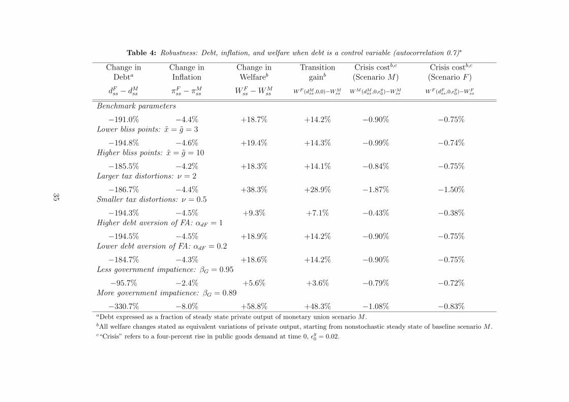
Table 4: Robustness: Debt, inflation, and welfare when debt is a control variable (autocorrelation 0.7)∗

Change in Change in Change in Transition Crisis costb,c Crisis costb,c

Debta Inflation Welfareb gainb (Scenario M) (Scenario F )

dFss − dMss πFss − πMss W Fss −WM

ss WF (dMss ,0,0)−WMss WM (dMss ,0,ε

g0)−WM

ss WF (dFss,0,εg0)−WF

ss

Benchmark parameters

−191.0% −4.4% +18.7% +14.2% −0.90% −0.75%Lower bliss points: x = g = 3

−194.8% −4.6% +19.4% +14.3% −0.99% −0.74%Higher bliss points: x = g = 10

−185.5% −4.2% +18.3% +14.1% −0.84% −0.75%Larger tax distortions: ν = 2

−186.7% −4.4% +38.3% +28.9% −1.87% −1.50%Smaller tax distortions: ν = 0.5

−194.3% −4.5% +9.3% +7.1% −0.43% −0.38%Higher debt aversion of FA: αdF = 1

−194.5% −4.5% +18.9% +14.2% −0.90% −0.75%Lower debt aversion of FA: αdF = 0.2

−184.7% −4.3% +18.6% +14.2% −0.90% −0.75%Less government impatience: βG = 0.95

−95.7% −2.4% +5.6% +3.6% −0.79% −0.72%More government impatience: βG = 0.89

−330.7% −8.0% +58.8% +48.3% −1.08% −0.83%aDebt expressed as a fraction of steady state private output of monetary union scenario M .bAll welfare changes stated as equivalent variations of private output, starting from nonstochastic steady state of baseline scenario M .c“Crisis” refers to a four-percent rise in public goods demand at time 0, εg0 = 0.02.

35

output. Greater tax distortions also increase the welfare cost of a fiscal crisis; but as

before, this cost is greater in scenario M than it is in scenario F (1.87% versus 1.5%

of private output in perpetuity).27 If we instead lower the tax distortion parameter to

ν = 0.5, all these effects are scaled down, but it remains true that establishing a fiscal

authority leads to a large welfare gain without creating a tradeoff against the costs of

stabilizing a crisis.28

Similar conclusions apply when we vary the government’s discount factor βG. De-

creasing βG to 0.89 hugely increases government debt, which makes the establishment

of a fiscal authority much more valuable.29 It also makes stabilizing a crisis more costly,

but less so in the presence of a fiscal authority than in the status quo monetary union.

Varying the debt aversion αdF of the fiscal authority has similar effects (in the opposite

direction), but quantitatively it is less important than βG, because all the values of αdF

considered result in low steady-state debt. Starting from the baseline parameterization

of scenario M , establishing a fiscal authority with αdF = 1 causes steady state debt to

fall from 199.7% to 5.2% of private output. If instead the authority’s debt aversion is

αdF = 0.2, steady state debt falls from 199.7% to 15.0% of private output; the welfare

implications are similar in both cases. Likewise, variations in the bliss points x and g

cause only mild quantitative changes in our results.

3.4 Games with debt as a residual

An additional robustness issue relates to the instruments that policy institutions control

in our model. The games considered thus far assumed that either the government or the

fiscal authority could unilaterally control time t debt issuance, and that public spending

would adjust as necessary to satisfy the budget constraint, given debt issuance and tax

revenues. While this assumption is not uncommon in macroeconomic models, it is

rather unrealistic. After all, standard budget procedures typically authorize spending

programs and set tax rates early in the fiscal year, issuing debt later in the budget cycle

as necessary to adjust for any unexpected imbalances. In such an environment, neither

the government nor a hypothetical independent fiscal authority controls debt so closely

as we have assumed. Therefore, in this section, we study how our previous results are

altered if debt is a residual. Concretely, we now assume that expenditure, inflation,

27Table 4 is directly comparable to Table 3, in which perturbations have autocorrelation 0.7.

28The table reports the costs of a one-time crisis, but similar results apply with respect to cyclicalcosts in the sense of Lucas (1987).

29In these examples we always assume that the impatience of the fiscal authority is intermediatebetween that of the government and society, βF = 0.5(βS + βG).

36

and taxes are control variables of the players in our game, while debt is the residual

variable that adjusts to ensure that the budget constraint is satisfied in equilibrium.

3.4.1 Institutional scenarios

Scenario Md: Status quo model of a large monetary union, with debt as a residual

We start by looking at a large monetary union, with a single central bank that

chooses inflation πt for the whole union, while J regional governments Gj each choose

regional taxes τjt and government expenditure gjt; djt is then given by the budget

constraint (5). Thus, the central bank’s choice set is ΘCt ≡ πt, dj,tJj=1, and gov-

ernment j’s choice set is ΘGjt ≡ τjt, djt, gj,t. As before, all policy makers act under

discretion. While previously the central bank recognized that high inflation implied

higher contempraneous output and public services, now it knows that raising inflation

raises output and lowers debt. This complicates its Euler equation, since it foresees

the impact of changing debt on other players’ choices in the next period:

απCπt + ν ¯xt = βSχdt−1 + κ

χdt + κEt

[(απCπt+1 + ν ¯xt+1)(R(dt) +R′(dt)dt) +

+

(1

ν+q2Lν

αgC

)(απCπt+1 + (1 + χdt + κ)ν ¯xt+1)

∂xt+1

∂dt+

+(χdtαπCπt+1 − ν ¯xt+1)∂πt+1

∂dt

]. (46)

Next, consider the Euler equation that governs fiscal policy over time. The govern-

ment still trades off its impact on public and private spending according to (26). Also,

we continue to focus on the limit of a large monetary union (J = ∞) in which each

individual country is infinitesimal, so government j ignores all the spillovers from its

decisions. Then its Euler equation simplifies to

xj,t = βGR(dt)Etxj,t+1. (47)

Previously, to calculate the symmetric solution of scenario M , we solved for two

policy functions. Now, equilibrium can be characterized by three policy functions:

gross borrowing dt = BMd(Ωt), inflation πt = IMd(Ωt), and the output deviation

XMd(Ωt) ≡ xt − x. Using (6), we can write the budget constraint and the Euler

equations as follows:

BMd(Ωt) = (β−1S + δdt−1)dt−1 + (1 + χdt−1)(Et−1[IMd(Ωt)]− IMd(Ωt)) +(1

ν+q2Lν

αgC

)XMd(Ωt)− κIMd(Ωt) + zt, (48)

XMd(Ωt) = βG(β−1S + δdt−1

)EtX

Md(BMd(Ωt), st, εt+1), (49)

37

απCIMd(Ωt) + νXMd(Ωt) =

βSχdt−1 + κ

χBMd(Ωt) + κ

[απCI

Md(BMd(Ωt), st, εt+1) + νXMd(BMd(Ωt), st, εt+1)] (β−1S + 2δBMd(Ωt)

)+(

1

ν+q2Lν

αgC

)[απCI

Md(BMd(Ωt), st, εt+1) + (1 + χBMd(Ωt) + κ)νXMd(BMd(Ωt), st, εt+1)] ∂XMd

∂dt(BMd(Ωt), st, εt+1)

+[χdtαπCI

Md(BMd(Ωt), st, εt+1)− νXMd(BMd(Ωt), st, εt+1)] ∂IMd

∂dt(BMd(Ωt), st, εt+1)

.

(50)

Finally, given BMd(Ωt),Md(Ωt), and XMd(Ωt), public spending calculated from (26).

Scenario Fjd: Delegation of the tax rate to regional fiscal authorities, with debt as a

residual

Next, we consider the effect of delegating control of taxes to an independent regional

fiscal authority Fj, while regional governments choose public spending. As before, the

central bank controls union-wide inflation. Debt is treated as a residual by all policy

makers, so ΘCt ≡ πt, dj,tJj=1, Θ

Gjt ≡ gj,t, dj,t, and Θ

Fjt ≡ τjt, djt. As in previous

policy games, we consider a symmetric equilibrium with many small countries.

The central bank’s decision problem is the same as in Scenario Md. But since taxes

and spending are now chosen by different policy makers, the linear equation (26) that

related output to public spending in previous scenarios no longer holds. Hence, the

central bank’s Euler equation is now given by

απCπt + ν ¯xt = βSχdt−1 + κ

χdt + κEt

[(απCπt+1 + ν ¯xt+1)(R(dt) +R′(dt)dt) +

+(αgC ¯gt+1(1 + χdt) + qL(απCπt+1 + ν ¯xt+1))∂ ¯gt+1

∂dt+

+

(1

ν

)(απCπt+1 + (1 + χdt + κ)ν ¯xt+1)

∂ ¯xt+1

∂dt+

+(χdtαπCπt+1 − ν ¯xt+1)∂πt+1

∂dt

]. (51)

Next, the region-j government Euler equation can be simplified to

gj,t = βGEt

[R(dt)gj,t+1 −

(qLαgG

xj,t+1 −1

νgj,t+1

)∂xt+1

∂dt

], (52)

and the regional fiscal authorities set taxes, or implicitly output, such that

νxj,t + αdFdj,t = βFEt

[νxj,t+1R(dt) + (qLνxj,t+1 − αgGgj,t+1)

∂gj,t+1

∂dt

]. (53)

38

The final equilibrium condition is given by the budget constraint. We must now solve

simultaneously for four policy functions: for the gross borrowing function, the inflation

function, and the output function, as in scenario Md, plus the policy function that

determines government expenditure, gt = GFjd(dt−1, st−1, εt).

Scenario Fd: Delegation of tax rates to a union-wide fiscal authority, with debt as a

residual

Finally, we consider delegating control of all regions’ taxes to a union-wide fiscal

authority, under the assumption that debt is a residual. The instrument allocation

is ΘCt ≡ πt, dj,tJj=1, Θ

Gjt ≡ gj,t, dj,t, and ΘF

t ≡ τjt, djtJj=1. As in scenario

Fjd, equilibrium is characterized by (51) for the central bank, and (52) and a budget

constraint for each regional government. Finally, (53) is replaced by an analogous

first-order condition for the union-wide fiscal authority:

ν ¯xt + αdF dt = βFEt

[ν ¯xt+1(R(dt) +R′(dt)dt)

+(qLν ¯xt+1 − αgG ¯gt+1

) ∂gt+1

∂dt− (απFπt+1 + ν ¯xt+1κ)

∂πt+1

∂dt

]. (54)

Here again we must solve for four policy functions simultaneously.

3.4.2 Results

The key messages from our previous analysis in which debt was a control variable

were (i) delegation of budget balance responsibilities to a national or union-wide fiscal

authority achieves a large reduction in debt, inflation, and tax burdens in steady state,

and thereby raises steady-state welfare and (ii) in response to a public demand shock,

the fiscal authority imposes greater austerity on impact than the status quo scenario

would imply, but the overall welfare cost of the shock is lower, because the presence of

the fiscal authority makes discretion less costly. Those conclusions remain true when

the control variable that may be delegated is taxes instead of debt. Figure 4 depicts the

policy functions; as before, fiscal authorities reduce debt and inflation relative to the

monetary union, but they do not allow as much smoothing of shocks (the borrowing

functions become flatter). As illustrated by Fig. 5, the inflation and debt responses

after a positive public spending shock are subdued by fiscal delegation, while output

falls more sharply. Again, the utility loss on impact is greater under a fiscal authority

than it is in the status quo monetary union, but the overall intertemporal welfare cost

of the shock is reduced by fiscal delegation, as we saw earlier in Fig. 3.

39

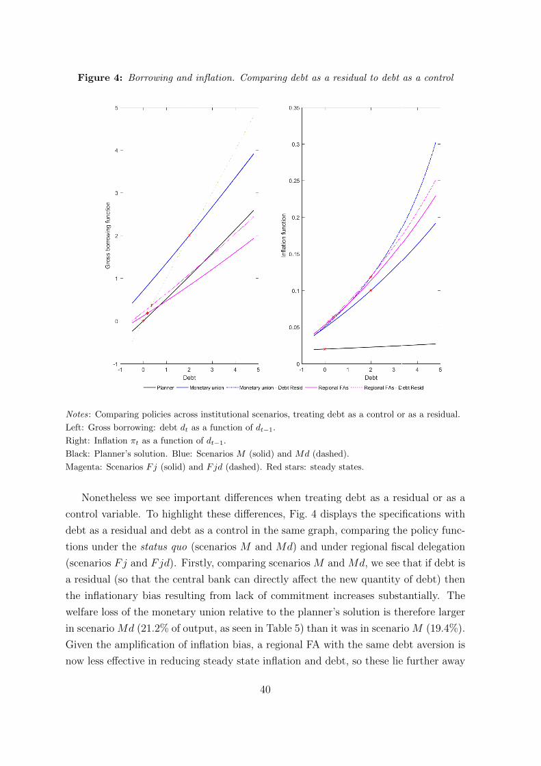
Figure 4: Borrowing and inflation. Comparing debt as a residual to debt as a control

Notes: Comparing policies across institutional scenarios, treating debt as a control or as a residual.

Left: Gross borrowing: debt dt as a function of dt−1.

Right: Inflation πt as a function of dt−1.

Black: Planner’s solution. Blue: Scenarios M (solid) and Md (dashed).

Magenta: Scenarios Fj (solid) and Fjd (dashed). Red stars: steady states.

Nonetheless we see important differences when treating debt as a residual or as a

control variable. To highlight these differences, Fig. 4 displays the specifications with

debt as a residual and debt as a control in the same graph, comparing the policy func-

tions under the status quo (scenarios M and Md) and under regional fiscal delegation

(scenarios Fj and Fjd). Firstly, comparing scenarios M and Md, we see that if debt is

a residual (so that the central bank can directly affect the new quantity of debt) then

the inflationary bias resulting from lack of commitment increases substantially. The

welfare loss of the monetary union relative to the planner’s solution is therefore larger

in scenario Md (21.2% of output, as seen in Table 5) than it was in scenario M (19.4%).

Given the amplification of inflation bias, a regional FA with the same debt aversion is

now less effective in reducing steady state inflation and debt, so these lie further away

40

from their optimal levels (comparing scenarios Fj and Fjd to the planner’s solution,

which is again shown in black). Therefore the welfare level achieved by fiscal delegation

is further from that of the planner’s solution in scenarios Fjd and Fd than it was in

scenarios Fj and F . Nonetheless, as a slightly less effective solution to a more serious

problem, the welfare gains from establishing a fiscal authority in a monetary union are

larger when debt is a residual (varying between 18.8% and 19.9% of private output, in

the four specifications reported in Table 5) than they were in our previous calculations

with debt as a control.

As for the effects of a public demand shock, Figure 5 graphs the effects of a 4%

increase in the public spending bliss point g, with autocorrelation 0.7, under the as-

sumption that debt is a residual, comparing scenarios P , Md, Fjd, and Fd. This

is comparable to Fig. 3, which studied the same shock but assumed that debt was a

control variable. The biggest quantitative differences between the specifications with

debt as a residual and as a control are seen in the output and inflation responses. The

fiscal authority reduces output more sharply in response to the shock in Fig. 5, where

it controls the tax rate, than it did in Fig. 3, where it was assumed to control debt

directly. On the other hand, because inflation bias is worse when debt is a residual,

the rise in inflation associated with the monetary union scenario Md (the blue curve

in Fig. 5) is greater than it was in scenario M (the blue curve in Fig. 3). Summing the

countervailing effects on output and inflation over time, public demand shocks are less

costly under the fiscal delegation scenarios Fjd and Fd than they are in the monetary

union scenario Md, as Fig. 5 and Table 5 both show.

4 Policy implications

Fear of moral hazard continues to hold back agreement on possible mechanisms to

prevent self-fulfilling attacks on Eurozone states’ sovereign debt (such as Eurobonds)

and cross-border panics in the European banking system (such as a Single Deposit

Insurance Mechanism). The basic problem is that any mechanism capable of prevent-

ing crises opens the door to irresponsible fiscal policies that count on future bailouts

instead of maintaining long-run national budget balance. Thus, designing an institu-

tional framework capable of ensuring long-run fiscal discipline is a crucial counterpart

to the establishment of crisis prevention mechanisms, so an adequate fiscal framework

could prove to be the key to the long-run stability of the Eurozone.

An independent fiscal authority for EMU

Our model points to a potentially powerful recipe for fiscal discipline: the establishment

41

Figure 5: Autocorrelated public demand shock. Comparing scenarios when debt is a residual.

Notes: Impulse responses of debt, inflation, government spending, output, and instantaneous and

cumulated utility to a 4% increase in the public spending bliss point g (autocorrelation ρ = 0.7),

assuming debt is a residual.

42

Table 5: Debt, inflation, and welfare in scenarios S where debt is a residual

Transition Crisis cost,b,c

Debta Inflation Welfareb gainb Crisis costb,c fixing debt Cyclical costb,d

dSss πSss W Sss −WM

ss WS(dMss ,0,0)−WMss WS(dSss,0,ε

g0)−WS

ss WS(0,0,εg0)−WS(0,0,0) WSss−WS

n (dSss,0,0)

Temporary shocks (autocorrelation 0)

Scenario P: Planner

0.1% 2.0% 21.2% +16.5% −0.39% −0.39% −0.12%Scenario Md: status quo monetary union

199.9% 11.8% 0% 0% −0.49% −0.43% −0.14%Scenario Fjd: Monetary union with regional fiscal authorities

36.4% 6.4% 18.8% +14.8% −0.40% −0.39% −0.12%Scenario Fd: Monetary union with union-wide fiscal authority

15.5% 5.9% 19.7% +15.2% −0.39% −0.39% −0.13%

Correlated shocks (autocorrelation 0.7)

Scenario P: Planner

0.1% 2.0% +21.2% +16.6% −0.75% −0.75% −0.86%Scenario Md: status quo monetary union

199.7% 11.8% 0% 0% −0.91% −0.83% −0.90%Scenario Fjd: Monetary union with regional fiscal authorities

36.4% 6.4% +18.9% +14.9% −0.76% −0.75% −0.74%Scenario Fd: Monetary union with union-wide fiscal authority

15.7% 5.9% +19.9% +15.4% −0.76% −0.75% −0.77%aDebt expressed as a fraction of steady state private output of baseline scenario M .bAll welfare changes stated as equivalent variations of private output, starting from nonstochastic steady state of baseline scenario M .c“Crisis” refers to a four-percent rise in public goods demand at time 0, εg0 = 0.02.dComparing stochastic economy with εgt ∼ N(0, 0.02) to nonstochastic economy (εgt ≡ 0).

43

of a budgetary agency within the European Commission, mandated to ensure long-run

budget balance, which for the sake of concreteness we will call the European Fiscal

Authority (EFA). What exactly would the EFA do? First, it would necessarily take

the form of a forecasting agency, monitoring and predicting fiscal trends in each member

state. Second, it could provide advice to member governments about the likely fiscal

impact of new policy proposals. These are tasks it would share with the national fiscal

councils that have been established in compliance with the “Fiscal Compact” treaty

(European Council, 2012).

Indeed, the “Five Presidents’ Report” (J. Juncker et al., 2015) has led to the cre-

ation of a similar monitoring council at the EU level. The new European Fiscal Board

will begin work in 2017, with a small staff and a mandate explicitly limited to moni-

toring and advice (European Commission, 19 October 2016). Nonetheless, if member

state governments wish it, this institutional seed could grow into something larger,

with expanded powers. Our concept of the EFA would go further, exercising execu-

tive control over one or more national fiscal instruments delegated to it by member

states. Importantly, these would have to be instruments with a sufficiently strong bud-

getary impact to give it effective control over the path of each member state’s public

debt. Our model suggests that by correcting biases caused by lack of commitment,

this setup would decrease debt accumulation, and might decrease the cost of economic

fluctuations even if it means that some shocks have sharper effects on impact.

In our model, all policy decisions are equilibrium outcomes of games between policy

makers with different instruments and preferences, representing different institutional

designs. Thus, our analysis is founded on the assumption that no policy makers can

truly commit to follow a rule, treating fiscal and monetary policies in a consistent way.30

Considering how pliable European fiscal rules have proved in practice, a model based

on discretion seems more informative than one based on commitment. But beyond

its role as a modeling device, we would also argue that granting discretion to fiscally

“conservative” institutions (in the sense of Rogoff, 1985) is a more realistic path for

Europe today than forever trying to make rules more binding. Just as independent

central banks may consider multiple short-run objectives while stabilizing inflation in

the long run, the EFA could take many short-run factors into account while nudging

its fiscal instrument(s) in the right direction to control debt in the long run. We em-

phasize long-run budget balance because avoiding permanent unidirectional transfers

30In our model, there is no equilibrium role for rules. An interesting extension would be a stochasticmodel of “sustainable equilibria”, which might allow us to incorporate rules and punishments asequilibrium outcomes, along the lines of Chari and Kehoe (1990). See Basso (2009) for an analysis ofmonetary delegation in a sustainable equilibrium model.

44

is essential to maintaining a long-run voluntary relationship between sovereign states.

This contrasts with the emphasis on uniform short-run deficit rules originally embodied

in the Maastricht Treaty of 1992, which have little justification in economic theory.

Likewise, we focus on strengthening the credibility of long-run budget balance rather

than centralizing fiscal decisions because the former seems a more realistic path for

Europe. Restricting the mandate of the EFA to fiscal sustainability leaves most fiscal

policy-making at the local level. Creating a federal government would instead centralize

fiscal policy, losing local information and hence decreasing the efficiency of spending.

Likewise, the decisions of a distant federal government might be perceived as less le-

gitimate and democratic. In this way, an unelected European body charged only with

ensuring long-run budget balance might actually produce a more democratic outcome

than would an elected European government with wider fiscal powers.

A credible quid pro quo

If we accept that this form of fiscal discipline is indeed beneficial, and compatible with

democracy, several further questions arise. First, is it politically feasible? Second,

can effective fiscal instruments be established, in practice? And finally, which fiscal

instrument(s) would be most appropriate for delegation to a hypothetical European

Fiscal Agency?

Although delegation of fiscal instruments is not standard practice today, it could

prove politically attractive in the current European context. Fiscally fragile countries

in the Eurozone still need backing from the monetary authorities in order to avoid

the risk of speculative attacks and banking panics, which the ECB is able to provide.

However, fiscally strong European countries oppose monetary protection against spec-

ulative attacks, because they fear moral hazard: the weaker countries might fail to

balance their budgets if they take ECB protection for granted.

These considerations point to a politically feasible quid pro quo. Let us suppose

that the mandate of the European Fiscal Board is expanded beyond an advisory role,

to ensuring long-run fiscal sustainability of member states by appropriately setting

the fiscal instruments that those member states choose to delegate to it. We will call

this hypothetical, more powerful agency the EFA. The first task of the EFA would

be to evaluate whether the instruments proposed for delegation by any given member

state are powerful enough and agile enough to give it effective control of that member

state’s debt. Once the EFA judges that it has been granted effective control of a

given member state’s debt level— including setting up the legal and administrative

framework for control of the proposed instruments by the EFA— then that member

45

state would become immediately eligible for ECB protection against speculative attacks

(by whatever mechanism the ECB judges appropriate).

Crucially, protection would remain contingent at all times on continuing approval

from the EFA. If at any time the EFA judges that its delegated instruments are less

powerful than expected, or if it judges that a member state has begun to “game the

system” in some way that makes it unable to control that state’s debt level, the EFA

would publicly revoke its approval of the delegated instruments (probably, but not nec-

essarily, after adequate advance warning to the member state). The ECB would then

be obliged to cease backing that state’s sovereign debt. One might question whether

it is credible to threaten to eliminate a member state’s protection against speculative

attacks. There could be scope for moral hazard if eliminating protection of the bonds

of one country caused contagion to others. But as long as the other fiscally fragile

countries are themselves participating in the EFA system, scope for contagion would

be greatly mitigated.

Which instruments to delegate?

Finally, we come to the question of which instrument(s), if any, would be appropriate

for delegating control of long-term budget balance to the European Commission. Our

paper has modeled instrument delegation in two ways. The simpler assumption is that

the fiscal authority actually issues each member state’s sovereign debt; the member

government is then free to spend the cash proceeds.31 We show that delegation of debt

issuance is very effective in reducing biases generated in a monetary union, theoretically

being the preferred option.

However, most forms of public spending involve long-term projects and long-term

contracts that are hard to adjust rapidly; therefore, in practice, most public spending

is planned long in advance, and sovereign debt issuance is typically a residual, chosen

after spending and taxes to compensate any difference between the two. Indeed, formal

control of debt issuance may not suffice for de facto control of the debt.32 The de facto

31When instead the authority is decreasing the debt stock in nominal terms, the implicit assumptionis that the fiscal authority is the first claimant on all period t tax revenues of region j until it achievesits desired debt level dj,t.

32A number of proposals, including Eichengreen, Hausmann, and von Hagen (1999), Wyplosz (2005),and Maskin (September 29, 2016), have advocated delegating the choice of a deficit limit, annually,to an independent fiscal authority. But this is better understood as delegating the choice of a target,rather than delegating an instrument. So this regime does not correspond to either version of ourmodel; instead, it is a game which requires discretionary action by the government, in a second stage,after the deficit limit is set, and therefore the debt level is not a control variable of the fiscal authority.

46

debt level may be affected by hidden securitization of future public revenues, by off-

balance sheet exposures (unfunded pensions, guarantees given to social security or

other state entities), or even by more explicit measures such as the issuance of scrip,

“platinum coins” (an instrument recently discussed in the US) or IOUs— or simply

delaying payments. These measures have in fact have been used quite frequently by

countries unable to formally issue more sovereign debt. Hence the second version of

our model assumes the fiscal authority controls taxes, instead of debt issuance per se.

While delegation is somewhat less effective in this case, it still significantly reduces

debt biases without imposing further constraints on stabilization.

An EFA could be granted control over taxes or government expenditure in a wide

variety of ways. In the case of taxes, probably the simplest idea is that of Gruen

(1997), who proposed defining a multiplicative shift factor in the Australian tax code.

He proposed applying this shift factor to income taxes, VAT taxes, and all other types

of taxes. Tax rates would take whatever complicated functional form the Australian

government chose, but would subsequently by multiplied by a factor Xt, which would

initially be set to one but would thereafter be adjusted by an independent fiscal au-

thority to ensure control of the debt level.

As for controlling government expenditure, Gomes (2011) argues that public sector

wages should optimally be state-contingent, rising in times of fiscal plenty and falling

when the budget is tight. Adjustments of this type would have a powerful budgetary

impact, and could in principle be performed very quickly, particularly if a shift factor

were spelled out explicitly ex ante in public contracts, instead of being an ad hoc crisis

response, as was the case in Spain and Portugal during the crisis. Additional adjust-

ment factors related to long-term budget trends offer another potentially powerful lever

that could be delegated to an independent fiscal authority. For example, in a recent

pension reform, the Spanish government established a “Factor de Revalorizacion An-

ual” that will be automatically adjust pensions each year in response to any persistent

deficits or surpluses in the pension system; see Sanchez (2014). However, any spending

adjustment that affects only part of the government budget could imply large distribu-

tional consequences across different groups in the population. Therefore, Costain and

de Blas (2012a,b), go a step further and point out that all public sector prices could be

made effectively state-contingent by budgeting them in an alternative unit of account,

the value of which could be determined by a fiscal authority.

Whether or not to participate in the EFA mechanism, and if so, which instrument(s)

to delegate to the fiscal authority, is ultimately a political decision that should be

taken democratically in each member state. But from the point of view of the political

quid pro quo between member states, the only essential question is whether a given

47

instrument has a sufficient budgetary impact to enable the EFA to adequately control

long-run debt. The only decision in the hands of the fiscal authority itself would be

the technical and quantitative question of what setting of its delegated instrument is

consistent with long-run budget balance under its forecasts, given the policies of the

member government.33 All other fiscal instruments would remain under the control of

the member government, consistent with the European principal of “subsidiarity”.

5 Conclusions

Motivated by the failure of fiscal rules to avoid deficit bias in Europe, this paper has

analyzed an alternative policy regime in which each member state government delegates

at least one fiscal instrument to an independent authority with a mandate to avoid

excessive debt. Other fiscal decisions remain in the hands of member governments,

including the allocation of spending across different public goods, and the composition

of taxation.

We have compared long run debt accumulation and the response to public spend-

ing shocks in dynamic games representing several different institutional configurations,

including a status quo monetary union scenario with many local governments, a mon-

etary union with a single federal government, and various fiscal delegation scenarios,

as well as a social planner’s solution. We made two simple assumptions to discipline

our treatment of different types of institutions: first, that elected institutions are rela-

tively impatient, and second, that an institution mandated to achieve a simple, feasible,

quantitative goal will value that goal more strongly than the rest of the society does.

In our numerical simulations, delegation of budget balance responsibilities to a

national or union-wide fiscal authority reduces debt, inflation, and tax burdens in

steady state, and thereby raises steady-state welfare, compared with the status quo

scenario. The welfare gains are large in our model, and it is plausible to suppose that

they could be large in practice too, because they are driven primarily by the fact that

a large change in steady-state debt implies a large reduction in the interest burden

on public debt, and hence on the burden of tax distortions. These conclusions hold

regardless of whether the fiscal authority chooses debt directly, or whether it instead

chooses the tax rate, implying that debt is determined as a budget residual.

33Since debt rather than deficits per se is the relevant issue for intertemporal budget balance, deficitsmay fluctuate substantially even when they are controlled by the EFA. There may even be circum-stances when a short-run deficit favors long-run budget balance, for example if a temporary deficitenables productive investments, or if the economy appears to be temporarily beyond the maximum ofits Laffer curve.

48

In response to a public spending shock, the fiscal authority imposes greater auster-

ity on impact than the status quo scenario would imply. Nonetheless, we find that the

overall welfare cost of the shock is lower under the fiscal authority, because its presence

makes lack of commitment less costly, so that paying back the initial debt increase is

much less distortionary. Similarly, the transition path when a fiscal authority is estab-

lished imposes substantial austerity as the high initial debt is paid down. Nonetheless,

the long-run welfare gains are so large that establishing a fiscal authority is preferred,

from an ex ante social welfare perspective, even when the economy starts at the high

steady-state debt level of the monetary union.

Going beyond the model, Section 4 discussed the role that fiscal delegation might

play in Eurozone reform, where a disciplined fiscal regime is a crucial counterpart (both

economically and politically) to most of the monetary and financial mechanisms cur-

rently under consideration to stabilize European economies and financial markets. A

European Fiscal Authority controlling at least one sufficiently powerful fiscal instru-

ment in a member state could guarantee that state’s long-run budget balance. The

member state itself would decide which instrument to delegate, while the EFA would

evaluate whether it is “sufficiently powerful”. Delegation to the EFA would be attrac-

tive if it made member states eligible for ECB protection against speculative attacks;

but even without such a guarantee it could be attractive as a way of improving fiscal

credibility and lowering risk premia. Therefore we have stressed that these institutions

could be constructed in a voluntary, step-by-step fashion. As long as fears of moral haz-

ard persist, peripheral countries can do little to achieve a union-wide agreement that

would protect them against any future shocks to the Eurozone. Reforming their fiscal

institutions— possibly unilaterally— is one way peripheral countries could jumpstart

the negotiations for such an agreement.

References

Alesina, A., and G. Tabellini (1987): “Rules and Discretion with Noncoordinated

Monetary and Fiscal Policies,” Economic Inquiry, 25(4), 619–30.

(1990): “A Positive Theory of Fiscal Deficits and Government Debt,” Review

of Economic Studies, 57(3), 403–14.

(2007): “Bureaucrats or Politicians? Part I: A Single Policy Task,” American

Economic Review, 97(1), 169–179.

Ball, L. (1997): “A Proposal for the Next Macroeconomic Reform,” Victoria Eco-

nomic Commentaries, 14(1), 1–7.

49

Basso, H. S. (2009): “Delegation, time inconsistency and sustainable equilibrium,”

Journal of Economic Dynamics and Control, 33, 1617–1629.

Basso, H. S., and J. Costain (2016): “Fiscal delegation in a monetary union with

decentralized public spending,” CESifo Economic Studies, Forthcoming.

Battaglini, M. (2011): “The Political Economy of Public Debt,” Annual Review of

Economics, 3(1), 161–189.

Beetsma, R. M., and H. Jensen (2005): “Monetary and fiscal policy interactions in

a micro-founded model of a monetary union,” Journal of International Economics,

67(2), 320–352.

Beetsma, R. M. W. J., and A. L. Bovenberg (1999): “Does monetary unification

lead to excessive debt accumulation?,” Journal of Public Economics, 74(3), 299–325.

Bergin, P. (1998): “Fiscal solvency and price level determination in a monetary

union,” Journal of Monetary Economics, 45, 37–53.

Broto, C., and G. Perez-Quiros (2013): “Disentangling contagion among

sovereign cds spreads during the european debt crisis,” Banco de Espana Working

Papers 1314, Banco de Espana.

Buti, M., W. Roeger, and J. In’t Veld (2001): “Stabilizing Output and Infla-

tion: Policy Conflicts and Co-operation under a Stability Pact,” Journal of Common

Market Studies, 39(5), 801–828.

Calmfors, L. (2011): “The Role of Independent Fiscal Policy Institutions,” CESifo

Working Paper Series 3367, CESifo Group Munich.

Chari, V. V., and P. J. Kehoe (1990): “Sustainable Plans,” Journal of Political

Economy, 98(4), 783–802.

(2007): “On the need for fiscal constraints in a monetary union,” Journal of

Monetary Economics, 54(8), 2399 – 2408.

(2008): “Time Inconsistency and Free-Riding in a Monetary Union,” Journal

of Money, Credit and Banking, 40(7), 1329–1356.

Costain, J., and B. de Blas (2012a): “The role of fiscal delegation in a monetary

union: a survey of the political economy issues,” Working Papers in Economic Theory

2012/11, Universidad Autonoma de Madrid.

50

(2012b): “Smoothing shocks and balancing budgets in a currency union,”

Moneda y Credito, 234, 37–91.

De Grauwe, P. (2012): “The Governance of a Fragile Eurozone,” Australian Eco-

nomic Review, 45(3), 255–268.

Debrun, X., D. Hauner, and M. S. Kumar (2009): “Independent Fiscal Agen-

cies,” Journal of Economic Surveys, 23(1), 44–81.

Dixit, A., and L. Lambertini (2003a): “Interactions of Commitment and Discretion

in Monetary and Fiscal Policies,” American Economic Review, 93(5), 1522–1542.

(2003b): “Symbiosis of monetary and fiscal policies in a monetary union,”

Journal of International Economics, 60(2), 235–247.

Eggertsson, G., and E. L. Borgne (2010): “A political agencies theory of central

bank independence,” Journal of Money, Credit and Banking, 42(4), 647–677.

Eichengreen, B., R. Hausmann, and J. von Hagen (1999): “Reforming Bud-

getary Institutions in Latin America: The Case for a National Fiscal Council,” Open

Economies Review, 10(4), 415–442.

Eichengreen, B., and C. Wyplosz (1998): “The Stability Pact: more than a

minor nuisance?,” Economic Policy, pp. 66–113.

European Commission (19 October 2016): “The European Fiscal Board: Questions

and Answers,” Press release, European Commission.

European Council (2012): “Treaty on Stability, Coordination, and Governance in the

Economic and Monetary Union,” .

Farhi, E., and I. Werning (2015): “Fiscal Unions,” Manuscript, Harvard Univer-

sity.

Gnocchi, S., and L. Lambertini (2016): “Monetary Commitment and the Level of

Public Debt,” Discussion paper.

Gomes, P. (2011): “Fiscal policy and the labour market: the effects of public sector

employment and wages,” European Economy - Economic Papers 439, Directorate

General Economic and Monetary Affairs (DG ECFIN), European Commission.

Gruen, N. (1997): “Making Fiscal Policy Flexibly Independent of Government,”

Agenda, 4(3), 297–307.

51

Gunter, S., D. Riera-Crichton, C. Vegh, and G. Vuletin (2016): “Non-linear

effects of tax changes on output: A worldwide narrative approach,” Manuscript,

Johns Hopkins University.

Hagemann, R. (2010): “Improving Fiscal Performance Through Fiscal Councils,”

OECD Economics Department Working Papers 829, OECD Publishing.

J. Juncker et al. (2015): “Completing Europe’s Economic and Monetary Union,” Eu-

ropean Commission.

Leeper, E. M. (1991): “Equilibria under ’active’ and ’passive’ monetary and fiscal

policies,” Journal of Monetary Economics, 27(1), 129–147.

Leeper, E. M., C. Leith, and D. Liu (2016): “Optimal Time-Consistent Mone-

tary, Fiscal and Debt Maturity Policy,” Working Papers 2016-04, Business School -

Economics, University of Glasgow.

Leith, C., and S. Wren-Lewis (2011): “Discretionary policy in a monetary union

with sovereign debt,” European Economic Review, 55(1), 93–117.

(2013): “Fiscal Sustainability in a New Keynesian Model,” Journal of Money,

Credit and Banking, 45(8), 1477–1516.

Lucas, R. S. (1987): Models of Business Cycles. Wiley-Blackwell.

Maskin, E. (September 29, 2016): “Should Fiscal Policy be Set by Politicians?,”

Seminar slides, ECB Annual Research Conference - Jean Monnet Lecture.

Mundell, R. (1961): “A Theory of Optimum Currency Areas,” American Economic

Review, 51(4), 657–665.

Obstfeld, M. (2013): “Finance at Center Stage: Some Lessons of the Euro Crisis,”

European Economy Economic Papers 493, European Commission.

Pisani-Ferry, J. (2012): “The Euro crisis and the new impossible trinity,” Policy

Contributions 674, Bruegel.

Rogoff, K. (1985): “The Optimal Degree of Commitment to an Intermediate Mon-

etary Target,” The Quarterly Journal of Economics, 100(4), 1169–89.

Sanchez, A. R. (2014): “The automatic adjustment of pension expenditures in Spain:

an evaluation of the 2013 pension reform,” Banco de Espana Working Papers 1420,

Banco de Espana.

52

Schoenmaker, D., and D. Gros (2012): “A European Deposit Insurance and Res-

olution Fund,” Working Document 364, CEPS.

Seidman, L. S., and K. A. Lewis (2002): “A New Design for Automatic Fiscal

Policy,” International Finance, 5(2), 251–84.

Sims, C. A. (1999): “The Precarious Fiscal Foundations of EMU,” De Economist,

147, 415–436.

(2013): “Paper money,” American Economic Review, 103, 563–584.

(September 20, 2012): “A least unlikely path to a sustainable EMU,” Seminar

slides, EABCN conference on “Fiscal and Monetary Policy in the Euro Area”.

Soros, G. (10 April 2013): “A European solution to the Eurozone’s problem,” Project

Syndicate.

von Hagen, J., and I. J. Harden (1995): “Budget processes and commitment to

fiscal discipline,” European Economic Review, 39(3-4), 771–779.

Wren-Lewis, S. (2002): “Fiscal policy, inflation, and stabilisation in EMU,” Mimeo,

Exeter University.

Wyplosz, C. (2005): “Fiscal Policy: Institutions versus Rules,” National Institute

Economic Review, 191(1), 64–78.

53

A Appendix: Deriving the Euler equations and com-

puting equilibrium

For each institution scenario considered, we construct a equilibrium in terms of the

state variables ~Ωt ≡ (~dt−1, ~st−1,~εt). To calculate the first-order conditions we must

initially allow for off-equilibrium deviations that would result in asymmetric states,

but ultimately we assume shocks are symmetric and solve for the resulting symmetric

equilibrium in terms of the reduced state Ωt ≡ (dt−1, st−1, εt). In this appendix, we

derive the functional equations that define the equilibrium policies for scenario M , and

then explain how we solve them. Our methodology is similar for other scenarios.

Scenario M treats debt, taxes, and inflation as controls, and public spending as a

residual. Thus, when we apply the generic decision problems (16)-(17) to scenario M ,

gj,t shows up in both the choice sets ΘCt and ΘGj

t :

Central bank: ΘCt = πt, gj,tJj=1

V C(~Ωt) =maxΘCt

−1

2

απCπ2t +

1

J

J∑j=1

(xj,t + ν(πt − πet − τj,t)− x)2

+ αgC (gj,t − gj,t)2

+ βCEtVC(~Ωt+1) +

1

J

J∑j=1

ΛCj,t[dj,t −

(R(dt−1

)+ χ(πet − πt)

)dj,t−1 + τj,t + κπt − qLgj,t

]. (55)

Regional government: ΘGjt = dj,t, τj,t, gj,t

V Gj(~Ωt) =max

ΘGjt

−1

2

απGπ2t +

(xj,t + ν(πt − πet − τj,t)− x

)2+ αgG (gj,t − gj,t)2

+ βGEtV

Gj(~Ωt+1) + ΛGjt[dj,t −

(R(dt−1

)+ χ(πet − πt)

)dj,t−1 + τj,t + κπt − qLgj,t

]. (56)

In equilibrium, each policy maker knows the strategies played by the others. To

make this explicit, we can write the decision problems showing that the variables not

chosen by C are instead given by Gj’s policy function, and vice versa. Hence, we define

Π(~Ωt) as the central bank’s inflation function, and Tj(~Ωt) as the tax policy function of

government Gj.

To write the Bellman equations precisely, we also write the gross borrowing function

of Gj as Bj(~Ωt), and we define the list of all country-specific borrowing functions,

~B(~Ωt) ≡ (B1(~Ωt), B2(~Ωt), . . . BJ(~Ωt)).

54

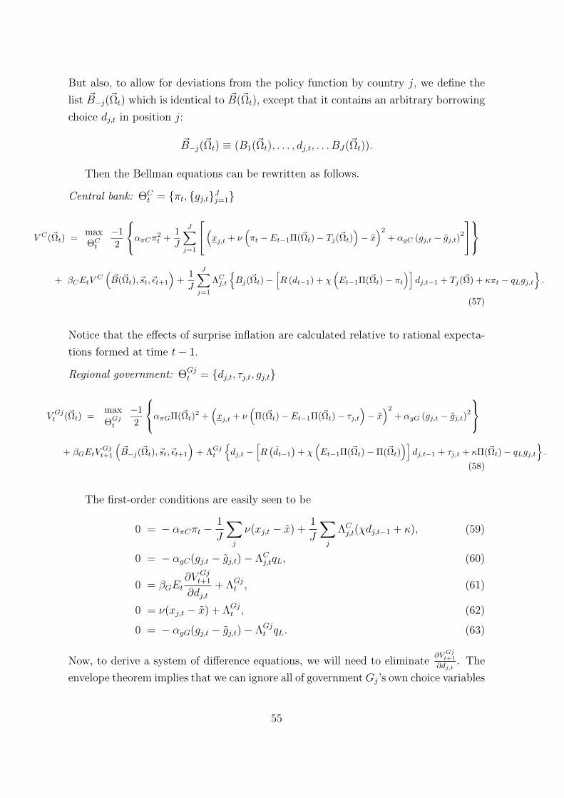
But also, to allow for deviations from the policy function by country j, we define the

list ~B−j(~Ωt) which is identical to ~B(~Ωt), except that it contains an arbitrary borrowing

choice dj,t in position j:

~B−j(~Ωt) ≡ (B1(~Ωt), . . . , dj,t, . . . BJ(~Ωt)).

Then the Bellman equations can be rewritten as follows.

Central bank: ΘCt = πt, gj,tJj=1

V C(~Ωt) =maxΘCt

−1

2

απCπ2t +

1

J

J∑j=1

(xj,t + ν(πt − Et−1Π(~Ωt)− Tj(~Ωt)

)− x)2

+ αgC (gj,t − gj,t)2

+ βCEtVC(~B(~Ωt), ~st,~εt+1

)+

1

J

J∑j=1

ΛCj,t

Bj(~Ωt)−

[R (dt−1) + χ

(Et−1Π(~Ωt)− πt

)]dj,t−1 + Tj(~Ω) + κπt − qLgj,t

.

(57)

Notice that the effects of surprise inflation are calculated relative to rational expecta-

tions formed at time t− 1.

Regional government: ΘGjt = dj,t, τj,t, gj,t

V Gjt (~Ωt) =max

ΘGjt

−1

2

απGΠ(~Ωt)2 +

(xj,t + ν

(Π(~Ωt)− Et−1Π(~Ωt)− τj,t

)− x)2

+ αgG (gj,t − gj,t)2

+ βGEtVGjt+1

(~B−j(~Ωt), ~st,~εt+1

)+ ΛGjt

dj,t −

[R(dt−1

)+ χ

(Et−1Π(~Ωt)−Π(~Ωt)

)]dj,t−1 + τj,t + κΠ(~Ωt)− qLgj,t

.

(58)

The first-order conditions are easily seen to be

0 = − απCπt −1

J

∑j

ν(xj,t − x) +1

J

∑j

ΛCj,t(χdj,t−1 + κ), (59)

0 = − αgC(gj,t − gj,t)− ΛCj,tqL, (60)

0 = βGEt∂V Gj

t+1

∂dj,t+ ΛGj

t , (61)

0 = ν(xj,t − x) + ΛGjt , (62)

0 = − αgG(gj,t − gj,t)− ΛGjt qL. (63)

Now, to derive a system of difference equations, we will need to eliminate∂V Gjt+1

∂dj,t. The

envelope theorem implies that we can ignore all of government Gj’s own choice variables

55

when calculating∂V Gjt

∂dj,t−1, but we cannot ignore the impact of dj,t−1 on other players’

choices. Thus we obtain

∂V Gjt

∂dj,t−1

= − ΛGjt

(R(dt−1) + χ(Et−1Π(~Ωt)− Π(~Ωt)) +

1

JR′(dt−1)dj,t−1

)−απGΠ(~Ωt)− κΛGj

t

∂Π

∂dj,t−1

−ν(xj,t − x)− χΛGj

t dj,t−1

( ∂Π

∂dj,t−1

− Et−1∂Π

∂dj,t−1

)+ βG

∑k 6=j

Et∂V Gj

t+1

∂dk,t

∂Bk

∂dj,t−1

. (64)

Taking expectations, the surprise inflation terms drop out. Therefore, (61) becomes

ΛGjt = βGEt

ΛGjt+1

(R(dt) +

1

JR′(dt)dj,t

)+απGΠ(B(~Ωt), ~st,~εt+1)− κΛGjt+1

∂Π

∂dj,t− βG

∑k 6=j

Et∂V Gjt+2

∂dk,t+1

∂Bk∂dj,t

.

(65)

In general, to evaluate this equation we would need to take another envelope condition

in order to eliminate the derivative∂V Gjt+2

∂dk,t+1. However, note that the factors ∂Π

∂dj,t,

∂V Gjt+2

∂dk,t+1

and ∂Bk∂dj,t

all scale proportionally to 1J

, while the summation operator in (65) scales

proportionally to J . Therefore, in the limit as J →∞, (65) reduces to

ΛGjt = βGR(B(~Ωt))EtΛ

Gjt+1, (66)

because all the other terms in the equation are of order 1J

. From here, simple algebra

leads to equations (28) and (30). Next, we restrict our calculations to the case of

symmetric shocks (εj,t = εt for all j), in which case the state of the economy can

be reduced from ~Ωt = (~dt−1, ~st−1,~εt) to the scalar triple Ωt = (dt−1, st−1, εt). We

therefore search for a symmetric solution, Bj(~Ω) = B(Ω) for all j, which must satisfy

the following functional equations:

BM(Ωt) = R (dt−1) dt−1 + (1 + χdt−1)[Et−1[IM(Ωt)]− IM(Ωt)

]− κIM(Ωt) + zt,

(67)

IM(Ωt) = βS(β−1S + δBM(Ωt)

)EtI

M(BM(Ωt), st, εt+1). (68)

We approximate the functions B(Ω) and I(Ω) with Chebyshev polynomials, and evalu-

ate the integral in (68) by Gauss-Hermite quadrature. We solve the model by searching

for Chebyshev coefficients such that (67)-(68) hold with sufficient accuracy.

56

A.1 Planner’s problem

Since the planner can commit, it can be viewed as choosing a plan, contingent on εt, for

each time t choice variable, including πt. Unlike the other environments, the equation

πet = Etπt not only holds as an equilibrium relation, but also enters as a constraint on

the planner’s problem. We will call the multiplier on this constraint λt. This multiplier

constrains the problem prior to the realization of εt, so in the planner’s solution it is

given by a function λt = λ(~dt−1, ~st−1) which does not depend on εt.

Solving problem (22), the following conditions must hold for any realization of the

shocks εt:

0 = − απSπt −1

J

∑νxj,t +

1

JΛPj,t(χdj,t−1 + κ)− λt (69)

0 = − αgS gj,t − ΛPj,tqL (70)

0 = βSEt∂V P

t+1

∂dj,t+

1

JΛPj,t (71)

0 = νxj,t + ΛPj,t (72)

dj,t = (R(dt−1) + χ(πet − πt))dj,t−1 + qLgj,t − τj,t − κπt (73)

πet = Et−1πt (74)

∂V Pt

∂dj,t−1

= − 1

JΛPj,t

(R( ¯dt−1) + χ(πet − πt)

)− 1

J2

∑k

R′(dt−1)dk,t−1ΛPk,t. (75)

By committing to πt as a function of εt, the planner is also committing (at t− 1) to an

expected inflation rate πet = Et−1πt. The first-order condition for πet is

0 = λt + Et−11

J

∑j

(νxj,t − χΛP

j,tdj,t−1

)gj,t. (76)

Simplifying, we see the usual intertemporal relation between x and g:

νxj,t =αgSqL

gj,t. (77)

Imposing symmetry to eliminate a covariance term, we can solve for λt:34

λt = −(1 + χdt−1)αgSqL

get , (78)

where get ≡ Et−1gt. Likewise, a symmetric equilibrium implies an Euler equation for

aggregate public spending:

gt = βS (R(dt) +R′(dt)dt)Etgt+1. (79)

34For comparability with our policy games, which were solved under the assumption of symmetricshocks to all regions at all times, we likewise solve the planner’s solution under a symmetric scenario.Therefore the planner’s policies depend on the ordered triple Ωt.

57

In contrast, there is no longer an analogous Euler equation for inflation, because

πt is shifted by the multiplier λt. Assuming symmetry, the first-order condition for

inflation is

−απSπt =αgSqL

(1 + κ+ χdt−1)gt + λt =καgSqL

gt + (1 + χdt−1)αgSqL

(gt − get ) . (80)

Note that λt is positive, and hence lowers the inflation rate πt chosen by the planner.

The inflation condition (80) can also be written as a relation between surprise inflation

and surprise public spending:

−απS (πt − πet ) =αgSqL

(1 + κ+ χdt−1) (gt − get ) (81)

The budget constraint for aggregate debt can be written as

dt = (R(dt−1 + χ(πet − πt))) dt−1 + (πet − πt) + q∗gt −καgSqLαπS

(1 + χdt−1)get + z, (82)

where

q∗ = qL +αgSqL

(1

ν2+

κ

απS(1 + κ+ χdt−1)

). (83)

We now have three equations, (79), (80), and (82), to solve for the three policy

functions G(Ω), B(Ωt), and Π(Ωt). Alternatively, we can eliminate inflation from the

budget constraint using (81):

dt = R(dt−1)dt−1 + (1 + χdt−1)(πet − πt) + q∗gt −καgSqLαπS

(1 + χdt−1)get + zt

= R(dt−1)dt−1 −αgSqLαπS

(1 + χdt−1)(1 + κ+ χdt−1) (gt − get ) + q∗gt −καgSqLαπS

(1 + χdt−1)get + zt

= R(dt−1)dt−1 +

(qL +

αgSν2qL

)gt +

κ2αgSqLαπS

get +αgSqLαπS

(κ2 − (1 + χdt−1)2) (gt − get ) + zt.

(84)

Now (79) and (84) suffice to determine the planner’s policies G(Ωt) and B(Ωt). The

relevant functional equations are:35

G(Ωt) = βS(β−1S + 2δB(Ωt)

)EtG(B(Ωt), st, εt+1), (85)

B(Ωt) = R(dt−1)dt−1 +

(qL +

αgSν2qL

)G(Ωt) +

κ2αgSqLαπS

Et−1G(Ωt)

+αgSqLαπS

(κ2 − (1 + χdt−1)2)(G(Ωt)− Et−1G(Ωt)

)+ zt. (86)

35A non-stochastic version of these two equations can be solved first, to find non-stochastic policyfunctions Gt(dt−1, st−1) and Bt(dt−1, st−1), which can then be used as an initial guess for solving thestochastic equations (79) and (84).

58