fiscal delegation in a monetary union ... - banco de españa

FISCAL DELEGATION IN A MONETARY UNION WITH DECENTRALIZED PUBLIC SPENDING

Henrique S. Basso and James Costain

Documentos de Trabajo N.º 1311

2013

FISCAL DELEGATION IN A MONETARY UNION WITH DECENTRALIZED

PUBLIC SPENDING

(*) Views expressed in this paper are those of the authors and should not be attributed to the Banco de España or the Eurosystem. The authors are grateful for helpful comments from Javier Andrés, Beatriz de Blas, Pablo Hernán-dez de Cos, Juan Francisco Jimeno, Bartosz Mackowiak, Albert Marcet, Javier Pérez, Giacomo Ponzetto, and seminar participants at CFE-ERCIM 2012, the Banco de España, the Bank of England, and the ECB-CFS Joint Lunch Seminar. The authors take responsibility for any errors.

Documentos de Trabajo. N.º 1311

2013

Henrique S. Basso and James Costain

BANCO DE ESPAÑA

FISCAL DELEGATION IN A MONETARY UNION

WITH DECENTRALIZED PUBLIC SPENDING (*)

The Working Paper Series seeks to disseminate original research in economics and fi nance. All papers have been anonymously refereed. By publishing these papers, the Banco de España aims to contribute to economic analysis and, in particular, to knowledge of the Spanish economy and its international environment.

The opinions and analyses in the Working Paper Series are the responsibility of the authors and, therefore, do not necessarily coincide with those of the Banco de España or the Eurosystem.

The Banco de España disseminates its main reports and most of its publications via the INTERNET at the following website: http://www.bde.es.

Reproduction for educational and non-commercial purposes is permitted provided that the source is acknowledged.

© BANCO DE ESPAÑA, Madrid, 2013

ISSN: 1579-8666 (on line)

Abstract

This paper studies the effects of delegating control of sovereign debt issuance to an

independent authority in a monetary union where public spending decisions are decentralized.

The model assumes that no policy makers are capable of commitment to a rule. However,

consistent with Rogoff (1985) and with the recent history of central banking, it assumes that

an institution may be designed to have a strong preference for achieving some clear, simple,

quantitative policy goal.

Following Beetsma and Bovenberg (1999), we show that in a monetary union where a single

central bank interacts with many member governments, debt is excessive relative to a social

planner’s solution. We extend their analysis by considering the establishment of an independent

fi scal authority (IFA) mandated to maintain long-run budget balance. We show that delegating

sovereign debt issuance to an IFA in each member state shifts down the time path of debt,

because this eliminates aspects of defi cit bias inherent in democratic politics. Delegating to

a single IFA at the union level lowers debt further, because common pool problems across

regions’ defi cit choices are internalized.

The establishment of a federal government with fi scal powers over the whole monetary

union would be less likely to avoid excessive defi cits, because only the second mechanism

mentioned above would apply. Moreover, the effective level of public services would be lower,

if centralized spending decisions are less informationally effi cient.

Keywords: fi scal authority, delegation, decentralization, monetary union, sovereign debt.

JEL classifi cation: E61, E62, F41, H63.

Resumen

Este trabajo estudia la delegación de la emisión de deuda soberana en una autoridad

independiente, en el contexto de una unión monetaria donde el gasto público se determina de

manera descentralizada. En el modelo, ningún agente puede comprometerse defi nitivamente

a seguir una regla. Pero, en línea con Rogoff (1985) y con la historia reciente de los bancos

centrales, el modelo supone que se puede diseñar una institución de manera que prefi era

cumplir con algún objetivo claro, concreto y cuantitativo.

Siguiendo el análisis de Beetsma y Bovenberg (1999), demostramos que el nivel de deuda

es excesivo (respecto a la solución de un planifi cador social) en una unión monetaria

donde un único banco central interactúa con muchos estados miembros. Extendemos el

modelo de Beetsma y Bovenberg para considerar el establecimiento de una autoridad fi scal

independiente (IFA en inglés) cuya meta es el mantenimiento del equilibrio presupuestario a

largo plazo. Demostramos que la delegación de la emisión de deuda soberana en una IFA

en cada estado miembro desplaza hacia abajo la senda temporal de la deuda. Esto se debe

a la eliminación de los factores del sesgo defi citario que son resultado de la política electoral.

Delegar la deuda soberana en una única IFA comunitaria disminuye aún más la deuda, al

internalizarse el problema de recursos en común entre los estados miembros.

Establecer un único gobierno federal para la unión monetaria tendría menos impacto

sobre el défi cit, porque se solucionaría el problema de recursos en común, pero no el del

sesgo defi citario de la democracia. Al mismo tiempo, el nivel efectivo de servicios públicos

proporcionado por el gobierno federal podría ser menor, debido a la menor efi ciencia de

información asociada con decisiones centralizadas.

Palabras clave: autoridad fi scal independiente, delegación de políticas, descentralización,

unión monetaria, deuda soberana.

Códigos JEL: E61, E62, F41, H63.

BANCO DE ESPAÑA 7 DOCUMENTO DE TRABAJO N.º 1311

1 Introduction

In the summer of 2012, when President Draghi expressed an unambiguous commitment

to preserve the Eurozone, returns on peripheral European debt plummeted. After

peaking at over 5%, premia on Spanish and Italian debt were both below 3% in early

2013,1 illustrating just how easily central banks can combat speculative attacks on

bonds issued in a currency they control. Since the ECB can, in principle, emit unlimited

quantities of euros, it can buy any quantity of euro-denominated debt, and thereby put

a floor under Eurozone sovereign bond prices. Nonetheless, further reforms are needed

to make Eurozone institutions viable in the long run. While the ECB can conjure

up a cap on the risk premium through monetary policy alone, this will eventually be

inflationary if peripheral countries fail to balance their budgets over the longer term.

Therefore a monetary mechanism to prevent speculative attacks must be accompanied

by an adequate fiscal regime if it is to ensure the permanence of the euro.

Proposals for fiscal reform have revolved around two competing interpretations of

“fiscal union”. Many economists and political leaders argue that it is time to con-

summate the founders’ vision of a strong federal Europe with a government able to

transfer resources countercyclically, from economies in expansion to those in recession.2

But European electorates are skeptical of placing more power in the hands of Brussels.

And core member states with healthy public finances have objected to a “fiscal transfer

union”, as they call it, because of the moral hazard it creates.3 Fearing that they could

end up paying for the fiscal imbalances of others, these members instead advocate a

“fiscal stability union”, meaning a reinforcement of the debt and deficit limits, backed

by monitoring and sanctions, that constituted the Stability and Growth Pact (SGP).

Unfortunately, there is no consensus about how to ensure that a rule-based framework

would succeed in the future, when so many member states broke the rules in the past.

However, it is wrong to assume that “fiscal transfer union” and “fiscal stability

union” are the only options for greater fiscal discipline in Europe. As a voluntary

association of nation states with large governments and distinct cultural identities,

the EMU is sui generis, and there is no reason to suppose that institutions which

1The Economist (19 January 2013).

2See for example Financial Times (8 December 2010), The Wall Street Journal (3 June 2011) orPisani-Ferry (2012).

3See The Economist (2 December 2010).


have succeeded elsewhere will be appropriate for Europe.4 While many countries suf-

fer budgetary problems today, fiscal indiscipline may be especially problematic in a

monetary union: member countries may overexploit the joint budget as a common re-

source; members may expect others to rescue them if they get into trouble; and market

doubts about any member’s solvency may spread contagiously across the union. For

all these reasons, members of a monetary union need strong fiscal regimes to ensure

long-run budget balance. But by itself this is not enough: beyond ensuring their own

solvency, peripheral Eurozone states must also convince core states that their solvency

is ensured. Otherwise, core members will be unwilling to help protect them from spec-

ulative attacks; and thus even if they slash deficits enough for solvency at low interest

rates, they will remain unprotected against a self-fulfilling spiral to higher rates at

which they become insolvent. This analysis suggests that the Eurozone requires much

stronger fiscal discipline than has been the norm in other economies.

This paper considers another way to reinforce fiscal discipline in Europe: the dele-

gation of executive control over one or more powerful fiscal instruments to an indepen-

dent institution with a mandate to ensure long-run budget balance. The motivation

for fiscal delegation follows from Rogoff’s (1985) analysis of central bank independence:

delegating discretionary control of monetary instruments can solve the problem of in-

flationary bias, without requiring an inflexible commitment to low inflation under all

circumstances, as long as the preferences of the central bank incorporate a counter-

vailing, anti-inflationary bias. Since the mandates of contemporary central banks are

strongly focused on low inflation, and since these banks control instruments that make

low inflation feasible, they have acted “conservatively” in Rogoff’s sense even in the

absence of formal rules relating to inflation only. Likewise, the establishment of an

independent authority with a mandate for low debt or low deficits might successfully

combat deficit bias, as long as it controls instruments of sufficient power to make debt

control feasible. While this idea has been largely absent from the current Eurozone

debate, frameworks like this have been proposed for many countries and regions, includ-

ing Australia and New Zealand (Ball (1996), Gruen (1997)); the US (Blinder (1997),

Seidman and Lewis (2002)); Latin America (Eichengreen, Hausmann, and von Hagen

(1999)); and the European Union (von Hagen and Harden (1995); Wren-Lewis (2002);

Wren-Lewis (2011); Calmfors (2003); Wyplosz (2005); Costain and de Blas (2012a)).

4In particular, in the short and medium run, we doubt that the US experience is informative forthe EMU, for two main reasons. First, the EMU has less consensus for political integration than theUS does; in fact, the crisis may be increasing the divisions between member states. Second, memberstates play a much larger fiscal role in the EMU than US states do, making a policy of zero deficitsat all times costlier (and less credible) for EMU members than it is for US states.


But while this idea has been widely advocated, there has been very little theoretical

work to evaluate the effects of policy delegation in a fiscal context.5

Thus, our model studies the effects of Rogoff-style delegation of fiscal powers in

the context of a monetary union. Our environment follows Beetsma and Bovenberg

(1999, henceforth BB99), who study the interaction of a single central bank with many

national (or regional) governments. Like Rogoff (1985), the BB99 paper posits a time-

inconsistency problem like that of Barro and Gordon (1983): a surprise increase in

inflation stimulates output, giving the central bank an incentive to choose an inflation

rate higher than the public expects. Inside a monetary union, this inflation bias also

gives rise to deficit bias by way of a common pool problem: while governments know

that the central bank will be tempted to inflate away the public debt, each individual

national government ignores the impact of its own debt, since this is only a small part of

the total. Therefore, BB99 conclude that welfare is improved if fiscal policy is bound by

rules limiting debt or deficits. But this analysis is built around a strange inconsistency:

it is unclear why they take for granted that the central bank must act under discretion

while assuming that the government’s fiscal decisions can (and advocating that they

should) be bound by a commitment to rules.6

Our paper strives for a more consistent treatment of rules versus discretion. We

assume that no policy makers can commit– that is, given the risk of unforeseen future

contingencies, no institution can irreversibly oblige itself to follow a rule. However,

consistent with Rogoff (1985) and with the recent history of central banking, we as-

sume that an institution may be designed to have a strong preference for achieving

some clear, simple, quantitative goal. Just as contemporary central banks display a

strong aversion to inflation, we consider a hypothetical independent budgetary author-

ity with a strong aversion to debt. We compare the baseline scenario of BB99, in

which the central bank has discretionary control of inflation and the government has

discretionary control of all aspects of fiscal policy, with an alternative institutional ar-

rangement in which the government controls the allocation of public spending, but an

independent fiscal authority controls the emission of debt. As BB99 already showed,

under the baseline scenario a monetary union with many member states exhibits ex-

cessive debt accumulation, relative to a social planner’s solution. We show in addition

5Persson and Tabellini (1994) explore a different aspect of fiscal policy delegation. They pointout that representative democracy is a form of policy delegation, and in line with Rogoff (1985),they argue that the median voter may prefer a representative with a relatively “conservative” view ofcapital taxation, in order to offset the problem of time inconsistency.

6Many papers written around the time of the introduction of the euro to provide theoretical backingfor the Stability and Growth Pact simply assumed that rules, once established, would be followed.See for example Buti, Roeger, and In’t Veld (2001).


that delegating control of debt issuance to an independent authority in each member

state decreases debt at all points in time. This follows from the greater debt aversion

and lower impatience of the fiscal authority, compared with a democratic government.

Delegating instead to a single independent authority at the level of the union shifts

down the time path of debt again, because a union-level authority internalizes common

pool problems associated with decentralized fiscal decisions. At the same time, this

alternative institutional setup maintains the advantages of subsidiarity, by leaving the

allocation of public spending to be decided at the national level, where information is

better and democratic legitimacy is greater.

In our baseline model, which follows BB99 closely, deficit bias in the monetary union

is a side-effect of inflation bias. Arguably, inflationary bias is not really relevant under

the current European monetary framework. However, other types of deficit biases, due

to moral hazard or contagion, might be present. Therefore, in Section 4, we extend

our model to include the possibility of contagion across governments’ borrowing rates.

We show that this contagion creates another form of deficit bias, also induced by a

common pool problem: each government feels the full benefit when it runs a higher

deficit, but the effect of higher debt on borrowing costs is shared across all members.

All results on the ranking of debt across different institutional regimes obtained in the

benchmark model continue to hold in the extended model with contagion.

While creating a new class of fiscal institutions might seem like an exotic remedy

for the Eurozone crisis, we feel our analysis provides grounds for optimism, because it

highlights a clear formula for political feasibility. Member states with precarious debt

levels would benefit from a European system to prevent speculative attacks. Mem-

ber states with strong finances fear providing this sort of guarantee precisely because

they worry that it would allow weaker members to continue running excessive budget

deficits. Therefore, a quid pro quo in which the ECB stops speculative attacks only for

countries that have adopted a truly credible budget balance regime appears politically

viable. The crucial point is that the fiscal regime must be solid enough to convince

core members that moral hazard has been eliminated. It is hard to see how any kind

of promise to follow a rule in all future circumstances, or how even the most savage

short-term austerity program, can really convince core members that moral hazard is

absent. This is why endowing an EU institution with instruments that give executive

control over national debt could prove to be the key to longer-term Eurozone survival.7

7See de Blas (7 June 2012, VoxEU) for details on institutional implementation.


1.1 Related literature

Economists have long emphasized the fiscal challenges implied by joining a monetary

union. Mundell (1961) argued that if a country gives up monetary independence,

it needs countercyclical fiscal policy to offset the amplified effects of asymmetric de-

mand shocks. More recent analyses focus on a more dramatic form of instability: by

giving up their ability to emit currency independently, member states (like emerging

economies that suffer from “original sin”) become vulnerable to speculative attacks on

their sovereign debt (Eichengreen and Wyplosz (1998); De Grauwe (2012)). Moreover,

this limits their ability to act as lenders of last resort for their domestic banks, so

troubles in the public and banking sectors become mutually reinforcing (Bruche and

Suarez (2010); Pisani-Ferry (2012)). The literature on monetary and fiscal interactions

(e.g. Leeper (1991); Sims (2013)) also points to the fragility of monetary unions: the

set of monetary and fiscal rules consistent with solvency and equilibrium determinacy

is likely to be reduced by joining a monetary union (Bergin (1998); Sims (1999); Leith

and Wren-Lewis (2011)). Another indication of fiscal vulnerabilities in a monetary

union comes from the literature on deficit bias. While Dixit and Lambertini (2003)

constructed an example in which joining a monetary union has no effect on policy

outcomes if all policy makers have identical objective functions, many other authors

argue that monetary union increases deficit bias when policy makers’ preferences differ

in plausible ways (Beetsma and Bovenberg (1999); Buti, Roeger, and In’t Veld (2001);

Beetsma and Jensen (2005); Chari and Kehoe (2007)).

Like inflation bias, deficit bias arises when policy makers are excessively impatient or

have incentives to break past promises; thus it is natural to ask whether Rogoff’s (1985)

proposal to combat inflation bias through policy delegation might also apply to deficit

bias. Like Rogoff, we model institutional differences parsimoniously by assuming differ-

ent weight parameters in their objective functions. First, we assume democratic politics

makes elected policy makers impatient (relative to society). This reflects widespread

findings in the political economy literature: for example, Alesina and Tabellini (1990)

show how alternating parties of opposing ideology may act impatiently, while Battaglini

(2011) shows how impatience may vary with the debt level, implying mean-reverting

dynamics like those of our extended model of Sec. 4. Second, we model the effects of a

policy mandate by placing extra weight on the mandated objective in the institution’s

preferences (relative to society).8 For a simple and quantifiable objective, this seems

8Adam and Billi (2008) show, in a microfounded New Keynesian model, that the benefits of“conservative” central banking extend to an economy with endogenous fiscal policy. Their modelshares some features with ours: they assume that the central bank’s preferences reflect those ofsociety, but place additional weight on inflation stabilization; and they consider the Markov perfectequilibria of a simultaneous game between monetary and fiscal policy makers, under discretion.


reasonable; central banks mandated to achieve low inflation do indeed appear to attach

great importance to this objective.9 Persson and Tabellini (1993) argue that central

banks might achieve better macroeconomic stabilization (and higher social welfare) if

they had more complex objectives in their mandates (or preferences). The tradeoff

between simple and complex objectives is an interesting issue, but probably requires

a deeper model of the effects of the mandate on institutions’ decisions. For the cur-

rent paper, which focuses on how systematic biases are affected by policy delegation,

Rogoff’s reduced-form approach provides useful insights.

Since the 1990s, as inflation fell and public debts grew in developed economies, many

economists have suggested delegating some fiscal responsibilities to an institution inde-

pendent of the government (see Debrun, Hauner, and Kumar (2009); Hagemann (2010);

and Costain and de Blas (2012a) for surveys), though few of these proposals have been

based on formal models. The literature distinguishes fiscal councils— which monitor

but do not implement fiscal policy actions— from independent fiscal authorities (IFAs),

which would make some of the fiscal decisions currently taken by the government. Fis-

cal councils are widespread today, and are mandated by recent European reforms,10 but

IFAs remain hypothetical. Two main types of IFA have been proposed. On one hand,

the IFA might set a deficit target, at the start of the annual budget cycle, which the

government is bound to respect; alternatively, it might exercise executive control over

some fiscal instrument with a strong budgetary impact.11 Some papers (see Hagemann

(2010), Sec. II.C; or Calmfors (2011), Sec. 1) take the nonexistence of IFAs today as

evidence of their inviability, arguing that delegation is less appropriate for fiscal than

for monetary policy since fiscal decisions are multidimensional, complex, and political.

However, the validity of this claim depends on which fiscal decisions are considered

(Alesina and Tabellini (2007) and Eggertsson and Borgne (2010) discuss what kinds of

decisions are appropriate to delegate from politicians to unelected technocrats). Our

model stresses the multidimensionality of fiscal policy, and envisions the delegation

of a single, quantitative decision to the IFA: the choice of the current deficit. This

9Alesina and Tabellini (2007) show that this may reflect the career concerns of the technically-skilled bureaucrats who lead them.

10See the “Fiscal Compact” treaty, European Council (2012). In accord with the treaty, the Spanishgovernment proposed legislation in June 2013 to establish a fiscal monitoring council; see Europa Press(28 June 2013).

11Proposals in the first class include von Hagen and Harden (1995); Eichengreen, Hausmann, andvon Hagen (1999); and Wyplosz (2005); those in the second class include Ball (1996); Gruen (1997);Seidman and Lewis (2002); Wren-Lewis (2002); and Costain and de Blas (2012a). Calmfors (2003)considers proposals of both types.


leaves the allocation of spending across different types of services (involving political

and distributional choices) within the democratic process.

In contrast, many high-profile calls for European monetary mechanisms to prevent

speculative attacks have assumed that this requires moves towards full political in-

tegration in Europe; see for example De Grauwe (2012), Soros (10 April 2013), and

Pisani-Ferry (2012). We agree that fiscal reforms are essential to backstop an enhanced

monetary policy, but we argue that the necessary reforms are much more limited than

is commonly supposed. What is essential is that European authorities have the ability

to ensure long-run national budget balance, and for this it suffices that they control at

least one fiscal instrument of sufficient power in each member state. In accord with the

principle of subsidiarity, the remaining fiscal decisions can remain at the national level.

Sims (September 20, 2012) has likewise stressed that fiscal discipline requires delegat-

ing from national governments to Europe some instrument with a strong impact on

each national budget, but that further fiscal integration is neither necessary nor likely

to prove politically feasible. Similarly, some limited European tax powers form an es-

sential backstop for the Schoenmaker and Gros (2012) framework for banking union,

but further fiscal integration is not required for their proposal.

2 The economic environment

The economic environment follows Beetsma and Bovenberg (1999, BB99) closely, but

is generalized to an arbitrary horizon T . Their paper, like Rogoff (1985) and Barro

and Gordon (1983), is built around a reduced-form model of the macroeconomy. Our

paper does not aim to explain the imperfections in public institutions’ decisions, such

as excessive impatience or deficit bias, which have been discussed extensively in the

political economy literature. Instead, our purpose is to build a model that incorporates

these features in a parsimonious way, in order to study how equilibrium outcomes differ

across games in which policy variables are controlled by different sets of institutions.

Our stripped-down model permits a detailed, analytical comparison of perfect foresight

equilibria across different policy regimes, to reveal how systematic policy biases are

damped or enhanced by different institutional configurations.12

12Our decision to study systematic biases analytically in a reduced-form model implies that we donot address the stabilization of shocks. Addressing optimal stabilization raises important additionalissues that are likely to require further microfoundations. These include the tradeoff between simpleand complex institutional objectives (Persson and Tabellini (1993)), and incentives that affect theoptimal speed of response to shocks, such as the impact of taxes on competitiveness in a monetaryunion (Leith and Wren-Lewis (2011)).


Time is discrete; we consider both finite- and infinite-horizon models. Several re-

gions j ∈ {1, 2, ...J} each benefit from local public spending, and face region-specific

budget constraints. These regions might be considered nations, or subnational areas.

Together, they form a monetary union, in which a single inflation rate applies.

2.1 Social welfare and budget constraints

Let time t private-sector output in country j be xj,t. We distinguish actual private

output from its target value xj,t (the bliss point). Our main assumption about the

macroeconomy is that actual output rises if inflation πt is higher than expected infla-

tion, πet , and that it falls with tax distortions τj,t:

xj,t = ν(πt − πet − τj,t). (1)

Social welfare decreases quadratically as output, inflation, and government services

gj,t deviate from their target values. The target level of inflation is assumed to be zero.

The loss function for region j is13

LSj =T∑t=0

βtS

{απSπ

2t + (xj,t − xj,t)

2 + αgS (gj,t − gj,t)2 .}

(2)

Here gj,t is the target level for government spending, and απS > 0 and αgS > 0

are weights representing the relative importance of deviations of inflation and public

services from their targets; without loss of generality the weight on output deviations

is set equal to one. The discount factor for social welfare is βS ≡ 11+ρS

< 1.

Since we are modeling a set of independent states that lack consensus for full polit-

ical integration, we assume that policy is constrained by a budget constraint for each

region. This takes the form

dj,t = Rdj,t−1 + pgj,tgj,t − τj,t − κπt, (3)

where dj,t is the real debt of region j at the end of period t (which must be paid off

at time t + 1). Our assumption that seignorage revenues κπt are linear in inflation,

independent of the debt level, effectively means that government bonds are issued in

real terms. If bonds were nominal, seignorage would also include a term proportional

to the product of inflation and debt. We make this assumption about seignorage

revenues for analytical convenience only; by optimizing a quadratic objective under

13Alesina and Tabellini (1987) derive an output relation of the form (1) from a more completemodel. Also, Leith and Wren-Lewis (2011) derive a social welfare function of the form (2) from astandard New Keynesian framework in which government spending enters the utility function.


linear constraints we can solve the model explicitly. But allowing for nominal debt

would only strengthen our results, since it would increase the gains from surprise

inflation, and thereby reinforce both the inflation and deficit biases in our model.

Note also that the real interest rate r is assumed constant, since quadratic pref-

erences imply certainty equivalence, so that R ≡ 1 + r represents the inverse of the

time-preference factor of the savers in the economy. Therefore, we impose the param-

eter restriction βSR = 1. Furthermore, if T is finite, then there is a final constraint

dj,T = 0 (4)

which simply says that the economy ends at time T , and therefore markets are unwilling

to make loans at T , since these loans will not be paid back. In an infinite-horizon

context, debt must instead respect the following “no-Ponzi” condition:

limt→∞

dj,tRt

≤ 0, (5)

which says that interest payments on debt are sufficient to make it worthwhile for the

private sector (with discount rate R−1) to hold the bonds.

Total public services in region j, gj,t, are a constant-elasticity aggregate of a variety

of differentiated services gj,k,t:

gj,t =

(∫ 1

0

ωj,k,t (gj,k,t)η−1η dk

) ηη−1

. (6)

where the ωj,k,t > 0 are weights on the different services k. Spending in region j is

financed by taxes in that region, τj,t, and by a share of seignorage revenues κπt. Total

government spending is a sum over all public goods,∫ 1

0gj,k,tdk. Spending is allocated

to minimize the cost of the public aggregate provided:

pgj,tgj,t ≡min

{gj,k,t}1k=0

∫ 1

0

gj,k,tdk s.t.

(∫ 1

0

ωj,k,t (gj,k,t)η−1η dk

) ηη−1

≥ gj,t (7)

Equation (7) serves to define the price of government services, pgj,t. We assume that

ωj,k,t is independently and identically distributed for all j, k, and t.

We consider two possible scenarios for the public spending decision. On one hand,

the policy maker that allocates public spending may know the distribution of ωj,k,t,

but not observe its realization. Then it is optimal to allocate spending equally across

all goods, so that

pgj,t = qH ≡ Eωη

η−1

j,k,t .


At the opposite extreme, the policy maker may observe wj,k,t before choosing gj,k,t.

In this case, it is optimal to allocate more spending to the most-demanded services,

according to the first-order condition

gj,k,tgj,l,t

=

(ωj,k,t

ωj,l,t

)η

This more efficient allocation makes aggregate public services less expensive:

pgj,t = qL < qH .

2.2 An omniscient, committed, cooperative Pareto planner

Given these objectives and constraints, we next establish a welfare benchmark for

our model. For relevance in the European context, we consider a Ramsey planner

who maximizes social welfare taking market equilibrium conditions and region-specific

budget constraints as given. Our planner does not represent any existing European

institution, as it has unrealistic advantages in information and decision-making, but it

represents a benchmark against which hypothetical institutions can be compared. For

this purpose, we study an omniscient, committed, cooperative Pareto planner :

• Omniscient : the planner observes ωj,k,t before choosing gj,k,t. This makes aggre-

gate public spending relatively inexpensive: pgj,t = qL.

• Commited : the planner can credibly commit to choose the inflation rate it has

previously announced. Therefore the inflation rate chosen by the planner is the

rate expected by the public: πt = πet .

• Cooperative: the planner chooses the policy variables for all regions j ∈ {1, ..., J},and thus internalizes any externalities across borders.

• Pareto: the planner obeys a distinct budget constraint for each region, maximiz-

ing social welfare insofar as this does not require transfers across regions.

We write the planner’s value function as VP,t, the maximized value of −LSj, summed

across all regions j. The value attainable depends on the debt levels of the regions,

according to the following Bellman equation:

VP,t

({dj,t−1}Jj=1

)=

maxπt, {dj,t, τj,t}Jj=1

−12

{απSπ

2t +

1

J

J∑j=1

[(ντj,t + xj,t)

2

+ αgS

(dj,t −Rdj,t−1 + τj,t + κπt

qL− gj,t

)2]}

+ βSVP,t+1

({dj,t}Jj=1

). (8)


The first-order conditions for inflation and for region-j taxes are

απSπt +1

J

J∑j=1

καgS

qL(gj,t − gj,t) = 0, (9)

ν (ντj,t + xj,t) +αgS

qL(gj,t − gj,t) = 0. (10)

At time T < ∞, the planner must obey the terminal condition (4), or if T = ∞ then

debt must satisfy (5). In all previous periods t < T , dj,t is chosen to satisfy

− 1

J

αgS

qL(gj,t − gj,t) + βS

∂VP,t+1

∂dj,t

({dk,t}Jk=1

)= 0. (11)

We can then use an envelope condition:

∂VP,t

∂dj,t−1

({dk,t−1}Jk=1

)=

1

J

RαgS

qL(gj,t − gj,t), (12)

to obtain an Euler equation for government spending in each region:

gj,t − gj,t = βSR(gj,t+1 − gj,t+1). (13)

Finally, the planner’s choices of taxes τj,t and debt dj,t determine current public services

gj,t through the period budget constraint:

dj,t = Rdj,t−1 + qLgj,t − τj,t − κπt. (14)

Two intratemporal properties of the planner’s solution are easily seen from the

first-order conditions. For each period and region, there is a fixed linear relationship

between output and public spending:

νxj,t =αgS

qLgj,t, (15)

where xj,t = xj,t − xj,t and gj,t = gj,t − gj,t and are the deviations of output and public

spending from their bliss points. There is also a constant linear relation between

inflation and average public spending:

απSπt = −καgS

qL¯gt, (16)

where ¯gt = J−1∑

j gj,t. Thus, inflation is positive as long as government spending is

below its bliss point, on average across countries.

Rewriting the Euler equation in terms of inflation, and plugging the within-period

relations (15)-(16) into the constraint (14), we obtain a simple difference equation

governing the aggregate dynamics of the planner’s problem:(dtπt+1

)=

(R −κP

0 1βSR

)(dt−1πt

)+

(10

)¯zt, (17)


where dt = J−1∑

j dj,t,¯zt = J−1

∑j(xj,t/ν + qLgj,t), and

κP = κ+απS

καgS

(q2L +

αgS

ν2

)(18)

If ¯z is constant, then the dynamics (17) have a steady state at zero inflation with

dss = −¯z

r. (19)

At this steady state, assets are so high (debt is so negative) that the bliss points of

output and public spending are affordable with interest earnings alone. The eigenvalues

around this steady state are R and (βSR)−1. Assuming that the second eigenvalue is

one, the system is saddle-path stable, and therefore has a unique equilibrium.

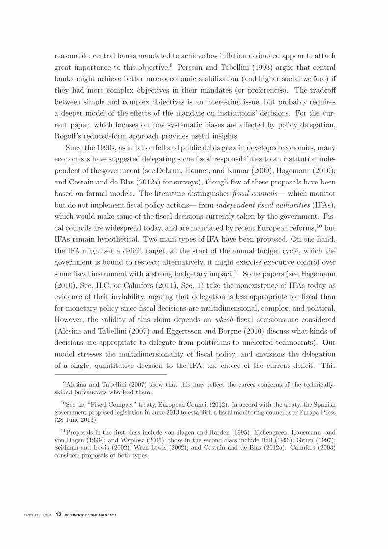
We can then summarize perfect foresight equilibrium behavior as follows.

• In an infinite horizon context, assuming βSR = 1, dSS is not the only steady

state. Instead, any debt level is a steady state (both in aggregate, and for each

region j separately).14 Debt is held constant by setting a constant inflation rate

π = (¯z + rd)/κP , thus smoothing seignorage distortions over time. (Likewise,

distortions in output and spending are smoothed over time in each country, at a

level consistent with unchanging debt.)

• In a finite horizon context, assuming βSR = 1, the planner smoothes seignorage

distortions over time by setting a constant inflation rate π. Inflation is chosen so

that aggregate debt hits zero at time T , dT = 0, given the aggregate constraint

dt = Rdt−1 − κPπ + ¯z. The required inflation rate is

π =1

κP

(¯z +

RT+1

RT+1 − 1rd−1

).

(Likewise, distortions in output and spending are smoothed over time in each

country, at a level consistent with dj,T = 0 for all j.)

3 Policy games

3.1 Policy makers’ objectives

Next, we consider equilibria in which several policy makers interact. Each one acts

to minimize a loss function that resembles (2), but they may have different discount

factors or different weighting coefficients on the loss terms.

14The existence of a continuum of steady states (or a random walk) for optimal debt is a standardfinding; see for example Benigno and Woodford (2003).


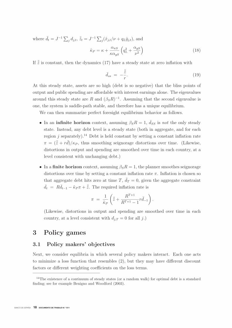
First, there is a central bank C, which chooses inflation for the whole monetary

union. The bank sums losses symmetrically across all J regions:

LC =T∑t=0

βtC

{JαπCπ

2t +

J∑j=1

[(xj,t − xj,t)

2 + αgC (gj,t − gj,t)2]} . (20)

Second, each region j has a government Gj which chooses each type of public spending

gj,k,t, and thereby chooses aggregate public spending gj,t. It may also be responsible

for choosing the tax rate, depending on the institutional scenario considered. The

government’s loss function LGj only reflects terms involving region j:

LGj =T∑t=0

βtG

{απGπ

2t + (xj,t − xj,t)

2 + αgG (gj,t − gj,t)2} . (21)

Third, we consider the possibility of a debt-averse fiscal authority. The fiscal au-

thority may be established by and for region j, in which case we will call it Fj, or it

may be a union-wide institution, in which case we will call it F . A regional authority

Fj is assumed to care only about regional variables, having the loss function

LFj =T∑t=0

βtF

{απFπ

2t + αdF

(dj,t − dj,t

)2

+ (xj,t − xj,t)2 + αgF (gj,t − gj,t)

2

}. (22)

This authority cares about the same terms as the society and government of region j,

but it also cares about the region’s real debt dj,t, suffering a loss if debt deviates from its

target value dj,t. The level of the target plays little role in the analysis, so we simply set

dj,t = 0. A debt term in the fiscal authority’s preferences is consistent with a mandate

for long-run budget balance, since respecting an intertemporal budget constraint means

that real debt cannot be too explosive. In contrast, the intertemporal budget constraint

says little about the time path of the deficit; indeed, optimal taxation theory highlights

the role of the deficit as a shock absorber, which may fluctuate strongly in order to

allow other, distorting instruments to be smoothed.

Alternatively, if there is a single union-wide fiscal authority, we assume that it sums

losses symmetrically across all regions:

LF =T∑t=0

βtF

{JαπFπ

2t +

J∑j=1

[αdF

(dj,t − dj,t

)2

+ (xj,t − xj,t)2 + αgF (gj,t − gj,t)

2

]}

(23)

Note that this function includes a separate term for each region’s debt, reflecting a

concern for budget balance in each individual region, above and beyond its concern for

union-wide budget balance. In other words, the fiscal authority is “Paretian”, like the

OCCPP planner.


Table 1: Baseline parameter assumptions

Society Central Government Fiscaland planner bank authority

Discount factor βi 0 < βS < 1 βC = βS 0 < βG < βS βG < βF ≤ βS

βSR = 1Spending coefficient αgi αgS > 0 αgC = αgS αgG = αgS αgF = αgS

Inflation coefficient απi απS > 0 απC > απS απG = απS απF = απS

Debt coefficient αdi αdS = 0 αdC = 0 αdG = 0 αdF > 0Coefficients of loss functions for agents i ∈ {S,C,G, F} .

3.1.1 Parameter assumptions

All these policy-making institutions are essentially benevolent, valuing the same goals

as society and the planner. However, their different roles may imply some differences

in priorities, reflected in the coefficients shown in Table 1. The central bank C and

the fiscal authority F have the same degree of patience as society, but the government

may be more impatient, due to the short time horizons of electoral politics. This is one

reason why the government’s decisions may exhibit deficit bias. All three institutions

i ∈ {C,G, F} value public spending to the same degree that society does. But the

central bank is assumed to have a mandate to achieve a target inflation rate; it therefore

weighs losses from inflation variability more strongly than society does.15 Likewise,

even though the debt level does not directly affect social welfare, we assume that the

fiscal authority has a mandate to stabilize debt around some target level, and that this

is reflected in its preferences. Therefore we include a positive coefficient on deviations

of debt from target in its objective function.

By themselves, the baseline parameter assumptions stated in Table 1 do not guaran-

tee the existence of an equilibrium with intuitively reasonable properties. This requires

some additional conditions.

• We say that governments exhibit moderate impatience when the discount rate

satisfies the following inequality:

βGR2 > 1. (24)

We will assume throughout that (24) holds, because otherwise the government’s

value function from (27) is unbounded in an infinite horizon context. In other

15Alesina and Tabellini (2007) discuss why society may prefer to delegate tasks with quantitative,verifiable objectives to bureaucrats, instead of leaving them up to the democratic government.


words, regardless of any other general equilibrium interactions, if (24) is not

satisfied, then the government’s partial equilibrium decision problem is not well

defined for the T =∞ case.

• We say that the central bank exhibits moderate inflation aversion when its pref-

erences satisfy the following inequality:

απC <1 + κ

καπS. (25)

Throughout Sec. 3, we will assume that (25) holds, because it is central to the

common pool problem of BB99, on which we base our model. As in Chari and

Kehoe (2007), governments anticipate that the central bank will adjust inflation

in response to their debt choices. If inflation rises more than is optimal when

debt increases (which is what moderate inflation aversion implies) then a single

government will hold down its debt in order to avoid the central bank’s inefficient

reaction; but as J →∞ this effect disappears, since each government regards its

own debt as negligible. We build on this particular common pool problem for

simplicity, and for consistency with BB99. But we will generalize to allow for

another version of the common pool problem in Section 4.

3.2 The game of BB99

Beetsma and Bovenberg (1999) assume that in period t, the central bank chooses πt,

while the governments choose τjt and djt. Each government then spends the resources

it has available, as given by the budget constraint (3). Market expectations are deter-

mined at the beginning of the period, rationally anticipating the outcome of the game

between the bank and the governments.

Each policy maker’s value is a function of the state of the economy, which includes

the debt of each region j. We search for an equilibrium in which no other state variable

is needed; that is, we rule out consideration of equilibria with more complex forms of

history dependence, such as reputational effects. We call the central bank’s value

function VC,t. Eliminating xj,t and gj,t using (1) and (3), its Bellman equation is:

VC,t

({dj,t−1}Jj=1

)=

maxπt

−12

{απCπ

2t +

1

J

J∑j=1

[(ν(πt − πe

t − τj,t)− xj,t)2

+ αgC


qL− gj,t

)2]}

+ βCVC,t+1

({dj,t}Jj=1

)(26)


Since policy makers cannot commit, this problem distinguishes between actual inflation

πt and expected inflation πet . Government j’s value VGj,t is governed by a similar

Bellman equation, which determines taxes and debt for country j:

VGj,t

({dk,t−1}Jk=1

)=

maxτj,t, dj,t

−12

{απGπ

2t + (ν(πt − πe


+ αgG


qL− gj,t

)2}

+ βGVGj,t+1

({dk,t−1}Jk=1

)(27)

The first-order condition for the central bank is

απCπt +1

J

J∑j=1

[ν (ν(πt − πe

t − τj,t)− xj,t) +καgC

qL(gj,t − gj,t)

]= 0. (28)

Compared with the social planner’s necessary condition (9), we see an additional term

relating to the central bank’s incentive to set inflation unexpectedly high. Government

j’s optimality condition for taxes is

−ν (ν(πt − πet − τj,t)− xj,t) +

αgG

qL(gj,t − gj,t) = 0. (29)

Like the social planner, the government must obey the terminal budget constraint (4)

or (5). For all periods t < T , government j sets

−αgG

qL(gj,t − gj,t) + βG

∂VGj,t+1

∂dj,t

({dk,t}Jk=1

)= 0. (30)

Its choices of taxes τj,t and debt dj,t then determine current spending gj,t according to

the period budget constraint:

dj,t = qLgj,t +Rdj,t−1 − τj,t − κπt. (31)

The presence of multiple policy makers of non-negligible size implies extra terms in

the value derivative in (30) which do not appear in the planner’s derivative (12). To

compute this derivative, we can ignore how dj,t impacts τj,t+1 and dj,t+1; these effects

have zero marginal value, by the envelope theorem. But we cannot ignore the fact

that changing dj,t will alter the central bank’s choice of πt+1, and other regions’ debt

choices dk,t+1, for k �= j; these interactions alter the marginal value of changing dj,t.

Differentiating (27), we obtain:

∂VGj,t

∂dj,t−1=

RαgG

qL(gj,t − gj,t)−

(απGπt +

καgG

qL(gj,t − gj,t)

)∂πt

∂dj,t−1+βG

∑k �=j

∂VGj,t+1

∂dk,t

∂dk,t∂dj,t−1

.

(32)


Note that we do not need to track how πet varies with dj,t−1. Any change in πe

t will

cancel with a corresponding change in πt, since under rational expectations πet = πt for

any value of dj,t−1.16 Next, yet another derivative appears in (32): the marginal effect∂VGj,t+1

∂dk,tof region k’s debt on government j’s value. Differentiating (27) again yields:

∂VGj,t

∂dk,t−1= −

(απGπt +

καgG

qL(gj,t − gj,t)

)∂πt

∂dk,t−1+ βG

∑l �=j

∂VGj,t+1

∂dl,t

∂dl,t∂dk,t−1

. (33)

Equations (28)-(29) are purely intratemporal, so they can be jointly simplified.

Assuming αgG = αgS, the relation between output and spending is the same as in the

social planner’s problem:

νxj,t =αgG

qLgj,t. (34)

Plugging (34) into (28), we can then calculate inflation in terms of the average deviation

of public spending from its bliss point:

απCπt = −(αgG + καgC

qL

)¯gt (35)

Comparing with the planner’s first-order condition (16), the right-hand side of (35)

contains an extra term reflecting the incentive for surprise inflation. On the other hand,

a high inflation aversion coefficient on the left-hand side tends to restrain inflation. We

can summarize the tradeoff between these two effects as follows:

• Under the baseline parameterization of Table 1, and assuming that the central

bank displaysmoderate inflation aversion, the BB99 equilibrium exhibits a higher

ratio of inflation to public spending distortions than the planner’s solution does.

3.2.1 Solution when J =∞Using the fact that value functions should be quadratic, and policy functions linear,

the model can be computed backwards for any J . But the solution is especially simple

if J = ∞ or if J = 1. First, neither inflation nor other regions’ debt will respond to

region j’s debt if region j is negligibly small. So when J =∞, (32) simplifies to

∂VGj,t

∂dj,t−1=

RαgG

qL(gj,t − gj,t) . (36)

Then, using (30) and (35), inflation obeys a very simple Euler equation:

πt = βGRπt+1. (37)

16Recall that, as in BB99, πet represents an expectation at the beginning of t, after time t−1 choices

and time t shocks have been revealed.


Summing debt across regions, the matrix dynamics of the model are(dtπt+1

)=

(R −κ0 1

βGR

)(dt−1πt

)+

(10

)¯zt, (38)

where dt and ¯zt were defined earlier, and

κ ≡ κ+(q2L +

αgG

ν2

) απC

αgG + καgC

. (39)

Notice:

• Assuming βG < βS, inflation grows faster in the BB99 economy than it does in

the OCCPP planning solution.

• Under the baseline parameterization of Table 1, κP > κ if and only if the central

bank exhibits moderate inflation aversion.

Both of these observations point to overaccumulation of debt in the BB99 economy.

First, faster inflation growth due to greater impatience means less inflationary financing

in the short run than in the long run, consistent with a short-run debt build-up, to be

paid off in the long run. Second, κP > κ shows that for any current pair (dt−1, πt),

if πt > 0, then the resulting debt level dt is lower in the social planner’s solution

than in the BB99 economy. This second effect, as we emphasized above, relies on the

assumption that the inflation aversion of the central bank is lower than optimal. As in

Chari and Kehoe (2007), this aspect of deficit bias is a side-effect of inflation bias.

Now, assuming ¯z is constant, these dynamics have the same steady state as the

social planner’s problem does, with zero inflation and debt level dss = − ¯zr. The

dynamics around the steady state are governed by the eigenvalues R and (βGR)−1,

which are both explosive. Therefore,

• In an infinite horizon context, no perfect foresight equilibrium with nonzero

bondholdings exists. With one predetermined variable (debt) and one jump vari-

able (inflation), existence of a (unique) infinite-horizon equilibrium would require

one stable and one unstable eigenvalue. Intuitively, the impatience of the govern-

ment is inconsistent with the discount rate of the bondholders in this economy,

so there is no infinite-horizon equilibrium in which the government’s debt is held.

• In a finite horizon context, inflation explodes at a constant rate over time, as

do output and spending distortions. That is, the impatient government chooses

low distortions initially; to pay off the resulting stock of debt, over time it must

increase inflation and taxes, while decreasing public services. The initial inflation

rate is chosen so that aggregate debt hits zero at time T , dT = 0, given the

aggregate dynamics dt = Rdt−1 − κπ + ¯z.


Focusing on constant ¯zt is reasonable, since our paper seeks to analyze systematic

deficit bias. When ¯zt is constant, we can show that the initial buildup of debt is

excessive, compared with the planner’s solution (see the appendix for the proof):

Proposition 1. Suppose T < ∞, J = ∞, βG < βS, and ¯zt = ¯z is

a constant. Then, starting from the same positive initial debt level

d−1 > 0, debt will be strictly higher at all times t ∈ {0, 1, ..., T − 1} in

the BB99 model than it is in the OCCPP planning solution.

3.2.2 Solution when J = 1

It is also relatively simple to analyze the case of a single region, J = 1. This case

is informative, since by comparing J = 1 with J = ∞ while holding other factors

fixed, we see the effects of joining a large monetary union. With only one region under

consideration, the last term of equation (32) drops out, and so (33) is not needed. We

can then derive the following Euler equation for public spending:

αgG

qLgt = βGR

αgG

qLgt+1 − βG

(απGπt+1 +

καgG

qLgt+1

)∂πt+1

∂dt. (40)

(The index j is suppressed here, since now there is only one region.) Using (35), we

can restate (40) in terms of inflation only:

πt = βG

(R + γ

∂πt+1

∂dt

)πt+1. (41)

where

γ = κ

(απG

απC

(αgG + καgC

καgG

)− 1

). (42)

We observe:

• Suppose the baseline parameter assumptions of Table 1 hold. Then γ < 1, and

γ > 0 if and only if the central bank displays moderate inflation aversion.

The matrix dynamics of the model are summarized by a system very similar to

those seen previously:(dtπt+1

)=

(R −κ0

[βG

(R + γ ∂πt+1

∂dt

)]−1)(

dt−1πt

)+

(10

)zt. (43)

Notice that moderate inflation aversion (γ > 0) will make inflation grow more slowly

for J = 1 than for J = ∞ as long as the central bank increases inflation in response

to greater debt (∂πt+1

∂dt> 0). Now, note that in this linear-quadratic model all control

variables should be linear functions of the states; and in particular, in an infinite-

horizon context ∂πt+1

∂dtwill simply be a constant. Lemma 1 states that moderate inflation

aversion suffices, but is not actually necessary, for this derivative to be positive.


Lemma 1. Suppose −κ2< γ. Then in any finite- or infinite-horizon perfect

foresight equilibrium of the BB99 game with J = 1, the response of

inflation to debt ∂πt+1

∂dtis positive at all times.

Given these results, we can now conclude that under moderate inflation aversion,

the model with a single region has lower inflation growth than the model with J =∞.

Since the κ term is the same in the J = 1 and the J = ∞ cases, the high inflation

growth of the J = ∞ case is associated with lower initial inflation, and higher final

inflation, and therefore implies that debt initially accumulates, to be paid off later

when inflation is high. Therefore:17

Proposition 2. Suppose βG < βS. Then:

(a.) A perfect foresight equilibrium exists when J = 1 if T <∞ or if γ is

sufficiently large.

(b.) Suppose T < ∞, and that the central bank exhibits moderate in-

flation aversion. Then, starting from the same positive per capita

debt level d−1 > 0, per capita debt will be strictly higher at all times

t ∈ {0, 1, ..., T − 1} if J =∞ than it would be if J = 1.

In other words, under moderate inflation aversion, a single region is less subject to

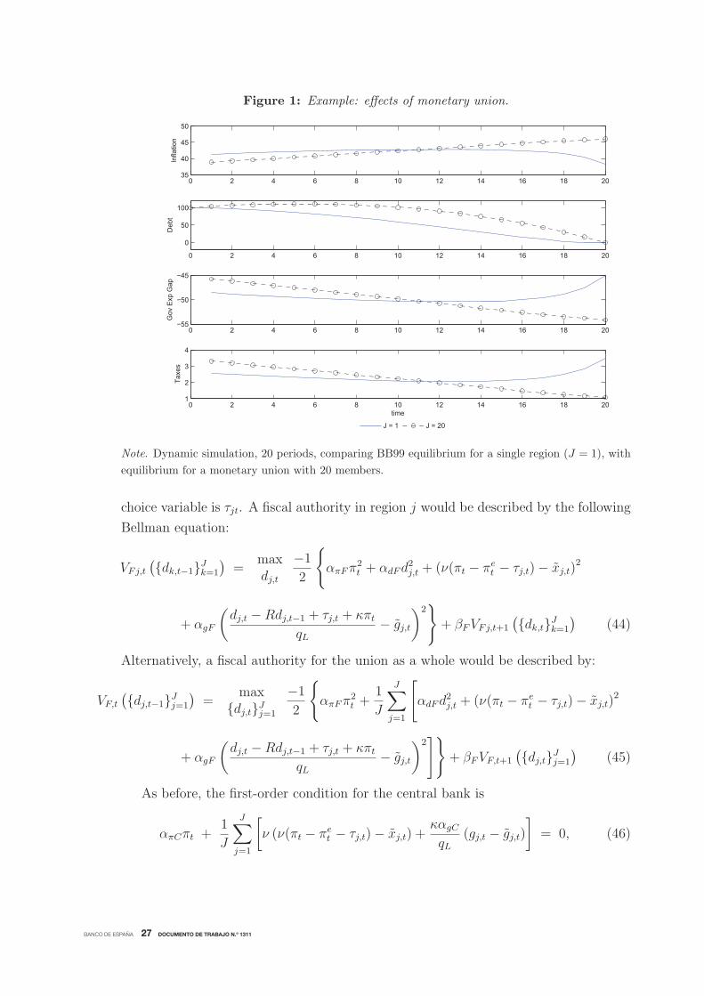
deficit bias than a monetary union (large J). This difference is illustrated for a finite-

horizon numerical example assuming “moderate impatience” and “moderate inflation

aversion”18, comparing J = 1 with J = 20, in Figure 1. We see that inflation, gov-

ernment services, and output vary less over time in the J = 1 economy, and that debt

declines roughly monotonically to zero by time T . In contrast, with J = 20, inflation

rises steadily with time, as a debt burden accumulates and then must eventually be

paid off; meanwhile government services and output decline steadily over time.

3.3 A game with a fiscal authority

Next, we solve a game in which debt is controlled by an independent debt-averse fiscal

authority. The central bank’s Bellman equation is given by (26), as in the BB99 game.

The Bellman equation of government j is identical to (27), except that now the only

17Result analogous to Prop. 2(b) are reported in the BB99 paper.

18The parameter values used in the numerical results are: βS = 0.96, R = 1/βS , ν = 1.94, q = 1,βG = 0.99βS , αgC = αgG = απG = 1, απC = 2 ∗ απG, x = −30, g = 100, d0 = 100 and d20 = 0.


Figure 1: Example: effects of monetary union.

0 2 4 6 8 10 12 14 16 18 2035

40

45

50

Infla

tion

0 2 4 6 8 10 12 14 16 18 20

0

50

100

Deb

t

0 2 4 6 8 10 12 14 16 18 20−55

−50

−45

Gov

Exp

Gap

0 2 4 6 8 10 12 14 16 18 201

2

3

4

Taxe

s

time

J = 1 J = 20

Note. Dynamic simulation, 20 periods, comparing BB99 equilibrium for a single region (J = 1), with

equilibrium for a monetary union with 20 members.

choice variable is τjt. A fiscal authority in region j would be described by the following

Bellman equation:

VFj,t

({dk,t−1}Jk=1

)=

maxdj,t

−12

{απFπ

2t + αdFd

2j,t + (ν(πt − πe


+ αgF


qL− gj,t

)2}

+ βFVFj,t+1

({dk,t}Jk=1

)(44)

Alternatively, a fiscal authority for the union as a whole would be described by:

VF,t

({dj,t−1}Jj=1

)=

max{dj,t}Jj=1

−12

{απFπ

2t +

1

J

J∑j=1

[αdFd

2j,t + (ν(πt − πe


+ αgF


qL− gj,t

)2]}

+ βFVF,t+1

({dj,t}Jj=1

)(45)

As before, the first-order condition for the central bank is

απCπt +1

J

J∑j=1

[ν (ν(πt − πe

t − τj,t)− xj,t) +καgC

qL(gj,t − gj,t)

]= 0, (46)


and government j’s necessary condition for taxes is

−ν (ν(πt − πet − τj,t)− xj,t) +

αgG

qL(gj,t − gj,t) = 0. (47)

Now suppose the fiscal authority is based in country j. Its terminal debt level must

satisfy the ”no Ponzi condition” (4) or (5) as in the previous models. In all periods

t < T it chooses debt to satisfy

−αgF

qL(gj,t − gj,t)− αdFdj,t + βF

∂VFj,t+1

∂dj,t

({dk,t}Jk=1

)= 0. (48)

Compared with the model of BB99, we notice that (48) includes a new, debt-related

term, derived from the fiscal authority’s debt aversion. Finally, the government’s tax

decision τj,t and the fiscal authority’s choice of debt dj,t jointly determine current

spending gj,t, via the period budget constraint:

dj,t = qLgj,t +Rdj,t−1 − τj,t − κπt. (49)

Since the players are not infinitesimal, each takes into account how its moves affect

future moves by other players. Thus, the fiscal authority’s marginal value of debt

includes its impact on future inflation and taxes, and on other regions’ future debts:

∂VFj,t

∂dj,t−1=

RαgF

qL(gj,t − gj,t) +

[ν(ν(πt − πe

t − τj,t)− xj,t)− αgF

qL(gj,t − gj,t)

]∂τj,t∂dj,t−1

−(απFπt +

καgF

qL(gj,t − gj,t)

)∂πt

∂dj,t−1+ βF

∑k �=j

∂VFj,t+1

∂dk,t

∂dk,t∂dj,t−1

=RαgF

qLgj,t −

(απFπt +

καgF

qLgj,t

)∂πt

∂dj,t−1+ βF

∑k �=j

∂VFj,t+1

∂dk,t

∂dk,t∂dj,t−1

(50)

The terms proportional to ∂τ∂d

cancel out of (50) using the baseline parameter assump-

tions from Table 1. Specifically, assuming αgG = αgF , they match the terms in the

government’s first-order condition (47), and therefore sum to zero. Evaluating (50)

also requires expressions for some cross derivatives, representing the marginal value to

Fj of region k’s debt, for k �= j. Again, the derivatives simplify if αgG = αgF :

∂VFj,t

∂dk,t−1=

[ν(ν(πt − πe

t − τj,t)− xj,t)− αgF

qL(gj,t − gj,t)

]∂τj,t

∂dk,t−1

−(απFπt +

καgF

qL(gj,t − gj,t)

)∂πt

∂dk,t−1+ βF

∑l �=j

∂VFj,t+1

∂dl,t

∂dl,t∂dk,t−1

= −(απFπt +

καgF

qLgj,t

)∂πt

∂dk,t−1+ βF

∑l �=j

∂VFj,t+1

∂dl,t

∂dl,t∂dk,t−1

. (51)


If instead the fiscal authority is a union-wide institution, for t < T it sets:

− 1

J

αgF

qL(gj,t − gj,t)− 1

JαdFdj,t + βF

∂VF,t+1

∂dj,t

({dk,t}Jk=1

)= 0. (52)

Using (45), the marginal value of country j’s debt is given by

∂VF,t

∂dj,t−1=

RαgF

qL

1

J(gj,t − gj,t)+

1

J

J∑k=1

[ν(ν(πt − πe

t − τk,t)− xk,t)− αgF

qL(gk,t − gj,t)

]∂τj,t∂dj,t−1

− 1

J

J∑k=1

(απFπt +

καgF

qL(gj,t − gj,t)

)∂πt

∂dj,t−1

=RαgF

JqLgj,t − 1

J

J∑k=1

(απFπt +

καgF

qLgj,t

)∂πt

∂dj,t−1. (53)

Here again, we have used αgG = αgF and (47) to eliminate the ∂τ∂d

terms. Notice

also that no value function derivatives occur on the right-hand side of (53); they are

eliminated using the envelope theorem.

The intratemporal first-order conditions can be simplified in the same way as in the

BB99 model. Equation (47) becomes

νxj,t =αgG

qLgj,t (54)

which is identical to (34). Likewise, plugging (54) into (46), we obtain:

απCπt = −(αgG + καgC

qL

)¯gt (55)

which is identical to (35).

3.3.1 Solving the FAj game when J =∞As in the BB99 model, calculating the value function derivatives generally requires a

numerical solution. But the main results can be seen by considering the limiting case

J = ∞, in which each region is infinitesimal, so neither inflation nor other regions’

debt will respond to region j’s debt. Then the envelope condition (50) simplifies to

∂VFj,t

∂dj,t−1=

RαgF

qL(gj,t − gj,t) . (56)

Plugging this expression into (48), we obtain an Euler equation for public spending:

αgF

qLgj,t + αdFdj,t = βFR

αgF

qLgj,t+1 (57)


Averaging across regions, we can write (63) in terms of inflation and average debt:

πt = αdF

(αgG + καgC

αgFαπC

)dt + βFRπt+1. (58)

Comparing (37) with (58), we see that the fiscal authority has two inflation-inhibiting

effects. First, at dj,t = 0, inflation grows more slowly in the presence of the fiscal

authority if βG < βF , that is, if the government is less patient than the fiscal authority.

Second, for any dj,t > 0 inflation grows more slowly in the presence of the fiscal

authority as long as αdF > 0, that is, if the fiscal authority dislikes debt.

The dynamics can be summarized in matrix form as(dtπt+1

)=

(R −κ−αβF

1+ακβFR

)(dt−1πt

)+

(1

− αβFR

)¯zt, (59)

where

α ≡ αdF

αgF

(αgG + καgC

απC

). (60)

We now summarize some key observations about these dynamics.

Prop. 3. Suppose the baseline parameter assumptions hold, and J =∞.

(a.) The model with a fiscal authority at the country level behaves exactly

as the BB99 model if βF = βG and αdF = 0.

(b.) If T = ∞ and βFR < 1, then no perfect foresight equilibrium ex-

ists if αdF = 0. A unique perfect foresight equilibrium exists if αdF is

sufficiently large.

(c.) Suppose T < ∞, βF > βG, αdF > 0, and ¯zt = ¯z is a constant. Then,

starting from the same positive initial debt level d−1 > 0, debt will be

strictly lower at all times t ∈ {0, 1, ..., T −1} in the regime with national

fiscal authorities than it would be in the BB99 model.

Prop. 3(a) points out that separating the choice of taxation and deficits from the

choice of spending has no effect if a local institution choosing taxes and deficits has

preferences identical to the government (because if so, the set of first-order conditions

defining equilibrium is equivalent).

To prove Prop. 3(b), we first show that both eigenvalues of the system (59) are real.

We then show that both eigenvalues are greater than one if αdF = 0, but that one of the

eigenvalues is less than one when αdF is sufficiently large. That is, sufficiently strong

debt aversion by the fiscal authority stabilizes debt dynamics, implying the existence

of a unique equilibrium. The condition for “sufficiently large” is:

αdF >1

κ

(απCαgF

αgG + καgC

)[R + βFR− βFR

2 − 1]. (61)


Condition (61) reduces to αdF > 0 if we impose βFR = 1, as in Table 1.

Part (c) is proved by relying again on the fact that the equilibrium policy functions

should be linear in debt. For T <∞, the coefficients of the linear function will change

over time, but they can be calculated by working backwards from the last period T . In

the appendix, we show that if the fiscal authority is less impatient than the government,

and/or exhibits debt aversion, then (starting from a positive debt level) debt always

remains higher in the BB99 economy than it does in the FAj economy.

3.3.2 Solving the FA game

Next, we solve the model with a single fiscal authority at the level of the monetary

union. To solve this case, note that given the linear form of the equilibrium, the

response of inflation to any given country’s debt must be 1/J times its response to

aggregate debt.19 Thus the envelope condition (53) becomes

∂VF,t

∂dj,t−1= =

1

J

RαgF

qLgj,t −

(απFπt +

καgF

qL¯gt

)1

J

∂πt

∂dt−1, (62)

so that the factor 1/J cancels out of the Euler equation:

αgF

qLgj,t + αdFdj,t = βFR

αgF

qLgj,t+1 − βF

(απFπt+1 +

καgF

qL¯gt+1

)∂πt+1

∂dt. (63)

We observe

• When debt is controlled by a single fiscal authority at the union level, the dy-

namics of the model are independent of the number of regions J .

If we now average over all regions, and substitute π for ¯g, we obtain the Euler

equation in terms of inflation:

πt = βF

(R + γF

∂πt+1

∂dt

)πt+1 + αdt, (64)

where α was defined in (60), and

γF = κ

(απF

απC

(αgG + καgC

καgF

)− 1

). (65)

We observe:

• Suppose the baseline parameter assumptions of Table 1 hold. Then γF = γ =< 1,

and γF > 0 if and only if the central bank displays moderate inflation aversion.

19This simplification would no longer be valid if we allowed for other parameter differences acrossregions, other than their initial debt level.


Writing the dynamics in matrix form, we have

(dtπt+1

)=

(R −κ−Rα

βF

(R+γF

∂πt+1∂dt

) 1+ακ

βF

(R+γF

∂πt+1∂dt

)

)(dt−1πt

)+

(1

− α

βF

(R+γF

∂πt+1∂dt

)

)¯zt.

(66)

This system combines two properties we have seen before. Like a model with fiscal

authorities at the regional level, debt alters the dynamics of inflation, as long as the

fiscal authority is debt averse (α > 0). But in addition, inflation growth is affected

by the term γF∂πt+1

∂dt, as in the BB99 model of a single region. This term is positive,

slowing down inflation growth, if the central bank exhibits moderate inflation aversion

and chooses ∂πt+1

∂dt> 0. Lemma 2 shows that inflation responds positively to debt in

the FA model under the same condition that applied to the BB99, J = 1 model.

Lemma 2. Suppose −κ2< γ. Then in any finite- or infinite-horizon perfect

foresight equilibrium of the FA game, the response of inflation to debt∂πt+1

∂dtis positive at all times.

Inflation growth is also slowed down, relative to the BB99 baseline model, by the

higher discount factor βF > βG. We summarize some key observations about system

(66) as follows.

Proposition 4. Suppose the baseline parameter assumptions hold.

(a.) The model with a single fiscal authority at the union level behaves

exactly as the BB99 model with J = 1 if βF = βG and αdF = 0.

(b.) If T =∞ and βFR ≤ 1, a unique perfect foresight equilibrium exists

if αdF is sufficiently large and/or if γ is sufficiently large.

(c.) Suppose T <∞, γF > 0, and ¯zt = ¯z is a constant. Then, fixing βF and

αdF and starting from the same positive initial debt level d−1 > 0, debt

will be strictly lower at all times t ∈ {0, 1, ..., T −1} under a union-wide

fiscal authority than it would be with national fiscal authorities.

Figure 2 shows a finite-horizon numerical example comparing the baseline BB99

scenario (with J = 20, as in Figure 1) and scenarios with regional or centralized fiscal

authorities assuming “moderate impatience” and “moderate inflation aversion”20.

20The parameter values used here are the same ones used in Figure 1. Additionally we set αdF = 0.1and βF = 0.995βS .


Figure 2: Example: effects of fiscal authority.

0 2 4 6 8 10 12 14 16 18 2030

40

50

Infla

tion

0 2 4 6 8 10 12 14 16 18 20

0

50

100

Deb

t

0 2 4 6 8 10 12 14 16 18 20−60

−50

−40

Gov

Exp

Gap

0 2 4 6 8 10 12 14 16 18 200

2

4

6

Taxe

s

time

Benchmark Union−wide FA Country FA

Note. Dynamic simulation, 20 periods, comparing three policy configurations for a monetary union

with 20 members: baseline BB99 equilibrium, equilibrium with fiscal authorities in each region, and

equilibrium with a single central fiscal authority.

3.4 A game with a federal government

Next, we briefly compare the behavior of an independent fiscal authority solely con-

cerned with budget balance with the behavior of a European federal government that

controls all aspects of fiscal policy. Given our specification of the previous games, it

now makes sense to assume that the budget constraint is

dj,t = Rdj,t−1 + qHgj,t − τj,t − sj,t − κπt. (67)

Government services now cost qH > qL, because taking all fiscal decisions at the union

level implies a loss of local knowledge about spending needs. The budget constraint

also reflects the possibility of transfers sj,t across regions. We could assume that the

government remains “Paretian”, so that regions remain fully responsible for their own

budgets, setting

sj,t = 0 (68)


for all j. But we could also consider a full “fiscal transfer union”, in which transfers

are constrained only byJ∑

j=1

sj,t = 0. (69)

The central bank’s Bellman equation now becomes:

VC,t

({dj,t−1}Jj=1

)=

maxπt

−12

{απCπ

2t +

1

J

J∑j=1

[(ν(πt − πe


+ αgC

(dj,t −Rdj,t−1 + τj,t + sj,t + κπt

qH− gj,t

)2]}

+ βCVC,t+1

({dj,t}Jj=1

)(70)

The government solves

VG,t

({dj,t−1}Jj=1

)=

max{dj,t, τj,t, sj,t}Jj=1

−12

{απGπ

2t +

1

J

J∑j=1

[(ν(πt − πe


+ αgG

(dj,t −Rdj,t−1 + τj,t + sj,t + κπt

qH− gj,t

)2]}

+ βGVG,t+1

({dj,t}Jj=1

)(71)

subject either to (68) or (69). Note that (71) is based on the assumption that the

European federal government is democratic. Consistent with our earlier assumptions,

we suppose that electoral politics tends to make the government more impatient than

society as a whole. And since the government must choose between many competing

uses of funds, there is no reason for it to be biased against debt, any more than an

individual region’s government would be.

Given our previous results, it is easy to see how this setup will behave. If the

government is Paretian, in the aggregate it acts just like our previous model of a single

government (with composite preferences) interacting with a single central bank. Thus

the dynamics are analogous to (43), except that they now refer to average debt over

the whole union:

(dtπt+1

)=

(R −κG

0[βG

(R + γ ∂πt+1

∂dt

)]−1)(

dt−1πt

)+

(10

)zGt . (72)

where

κG ≡ κ+(q2H +

αgG

ν2

) απC

αgG + καgC

, (73)

zGt ≡ qH gt +xt

ν. (74)


Note that these dynamics are independent of the number of regions, because the federal

government acts as a single decision-maker that internalizes the common pool problem

across regions. This is why the term γ ∂πt+1

∂dtappears in the inflation dynamics, as it does

in the BB99 model with J = 1, slowing down the explosion of inflation by counteracting

the impatience of the government.

A major disadvantage of this setup is the loss of “subsidiarity”: spending decisions

are taken at the union level, where less information is available, and therefore public

services are more expensive than they would be if they were allocated locally. The

relation between inflation, public spending, and output would be

¯gt = −(

απCqHαgG + καgC

)πt, (75)

xj,t = −αgG

ν

(απC

αgG + καgC

)πt (76)

Comparing with the corresponding relations for the BB99 economy, (34)-(35), which

also apply in the economy with a fiscal authority, (75) and (76) show that the relation

between inflation and output is unchanged, but that for any given level of inflation,

the distance of government services from their bliss point is increased.

We can summarize these observations as follows.

• Like a union-wide fiscal authority, a federal government for the monetary union

would internalize the common pool problem across regions. On the other hand,

the federal government would tend to accumulate more debt insofar as democratic

politics makes it more impatient and less debt averse than the fiscal authority.

• For a given level of inflation, the federal government would achieve the same

level of output, but a lower level of government services, compared with the fiscal

authority (and with the BB99 economy).

Intuitively, three forces restrain debt in the union-wide fiscal authority case: in-

creased patience, debt aversion and elimination of the common-pool problem. In the

federal government case, only the last of these three mechanisms applies. But beyond

the effects on the debt level, the federal government also causes a decrease in the ef-

ficiency of public spending, insofar as less information is available at the centralized

level for correctly allocating spending decisions.


3.4.1 Fiscal transfer union

If we instead consider a “fiscal transfer union”, in which nonzero transfers across regions

occur, the aggregate dynamics are still given by (72). The only difference is at the

regional level, at which all differences in distortions are eliminated. That is, gj,t and

xj,t are equalized across all regions, so that the marginal utilities of output and public

spending do not differ with j. This raises the level of social welfare in the aggregate,

but it is not a Pareto improvement: regions with higher debt (or less favorable shocks

gj,t or xj,t) benefit at the expense of regions with less debt or more favorable shocks,

from whom they receive transfers.21

4 Contagion and the common pool problem

Up to this point, our analysis has been based on a particular form of the budgetary

common pool problem, taken from BB99 and Chari and Kehoe (2007), in which deficit

bias arises only as a side-effect of inflation bias. Conveniently, this resulted in a linear-

quadratic model that we were able to characterize analytically in some detail. But

assuming that the central bank is insufficiently inflation averse does not seem like a

realistic description of the institutional setup in Europe. Therefore, in this section

we introduce a new form of the budgetary common pool problem, based on a more

appealing mechanism: contagion in sovereign bond markets. Realistically, we now

assume that the interest rate on sovereign bonds varies with the debt level. Outside

of a monetary union, we suppose that each country’s sovereign interest rate depends

only on its own debt. Inside a monetary union, we assume contagion increases: each

member state’s interest rate depends on its own debt, but also on the debt levels of the

other members. We model this contagion in the simplest and starkest way by treating

the interest rate throughout the monetary union as a function only of the average debt

level in the union.

This type of interest rate contagion implies a common pool problem in the monetary

union. A country with its own monetary policy would try to avoid debt accumulation,

in order to avoid an increase in the interest rate it pays. But a member of a large

monetary union knows that its debt is only an infinitesimal part of the total, and

therefore has no incentive to restrain its own debt accumulation even though a rise in

the union’s total debt raises interest rates for all. Under this assumption, “moderate

inflation aversion” of the central bank is no longer a necessary condition for inefficient

21Since the transfers sj,t are lump sum, only the present discounted value of transfers is determinedby the model, not the actual time path of transfers.


excess debt in the monetary union. An independent fiscal authority’s restraining effect

on debt is therefore additionally beneficial in this context.

When we build these effects into our model, the optimization problems of the plan-

ner, the central bank, the governments, and the fiscal authority (or authorities) are

identical to those considered in Section 3, except that now the interest rate varies with

debt, instead of being a constant r ≡ R − 1. For a country j with an independent

monetary policy, the interest rate on time t debt dj,t is

rj,t ≡ R(dj,t)− 1, (77)

where R is an increasing function. In a monetary union, the interest rate on all coun-

tries’ debt is instead

rt ≡ R

(J−1

J∑j=1

dj,t

)− 1. (78)

We will impose one weak restriction on debt and interest rates in equilibrium. We

say that the model exhibits extreme dynamic inefficiency if, at the steady-state debt

level dss,

R(dss) +R′(dss)dss ≤ 1. (79)

This condition cannot hold unless d is sufficiently low, so that d < 0 and/or R < 1; if it

holds, this means assets are so large that saving less in steady state would imply more

interest income in steady state. Since we are focusing our study on economies with

excessive debt, the extreme excess saving implied by (79) is of little interest. Therefore

we simply rule out any parameterization that implies (79).

The first order conditions are analogous to those seen previously. The equation

systems for the planner, for the individual country case (BB99, J = 1), for the monetary

union without a fiscal authority (BB99, J =∞), for the monetary union with country-

level fiscal authorities (FAj), and for the monetary union with a union-wide fiscal

authority (FA), are as follows.

Social Planner - OCCPP {dt = R(dt−1)dt−1 − κPπt + ¯zπt = βS

(R(dt) +R′dt

)πt+1.

(80)

BB99 - J = 1 {dt = R(dt−1)dt−1 − κπt + ¯z

πt = βG

(R(dt) +R′dt + γ ∂πt+1

∂dt

)πt+1.

(81)

BB99 - J =∞ {dt = R(dt−1)dt−1 − κπt + ¯zπt = βGR(dt)πt+1.

(82)


FAj - J =∞ {dt = R(dt−1)dt−1 − κπt + ¯zπt = αdt + βFR(dt)πt+1.

(83)

FA - J =∞ {dt = R(dt−1)dt−1 − κπt + ¯z

πt = αdt + βF

(R(dt) +R′dt + γ ∂πt+1

∂dt

)πt+1.

(84)

where R′ ≡ ∂R(J−1∑J

j=1 dj,t)∂dt

. We have not written these systems in matrix form, be-

cause they feature nonlinear interactions between inflation and debt. Using the budget

constraint, it is easy to show the following helpful fact:

Lemma 3. Consider any of the games defined by (80)-(84), and suppose

the model is not extremely dynamically inefficient. Then in any infinite-

horizon perfect foresight equilibrium the response of inflation to debt ∂π∂d

is positive at any stable steady-state debt level.

Comparing (81) with (82), we now see two distinct common pool problems. A single

government takes account of two effects of debt accumulation. Greater debt gives the

central bank a stronger incentive to create inflation, reflected in the term γ ∂π∂d, which

is positive at steady state, given Lemma 3, as long as the central bank is moderately

inflation averse (implying γ > 0). Also, greater debt implies a higher interest rate next

period, reflected in the term R′(d)d > 0. Both of these terms reduce inflation growth.

When there are multiple countries (of equal size), each country’s debt affects average

debt in proportion 1/J , so these terms are scaled down by the factor 1/J . In the limit

as J → ∞, these terms disappear, as we see in (82) and (83). The reduction of these

terms as J increases means that inflation growth increases with J (that is, deficit bias

rises with J), which is how the common pool problem is manifested here. While in the

baseline model there is a common pool problem only when γ > 0, with the additional

effect of interest rate contagion there remains a common pool problem even if γ is zero

or is mildly negative.

As before, the economies with fiscal authorities are equivalent to economies without

fiscal authorities under a particular parameterization. When βF = βG and αdF = 0

(which implies α = 0) the union with country level fiscal authority collapses to the

BB99, J = ∞ case, and the union with union-wide fiscal authority collapse to the

BB99, J = 1 case. Thus, propositions 3(a) and 4(a) continue to hold in the extended

model; and the parameterization under which fiscal authorities are neutral provides

a starting point for analyzing the effects of fiscal authorities under more interesting

parameterizations.


An advantage of the extended framework with a variable interest rate is that we

no longer need to focus the analysis on a finite-horizon context. When comparing the

regimes in our benchmark model, we focused on the path of debt for T < ∞, since

in many cases an infinite horizon solution did not exist. In the extended framework,

with interest rates that increase with debt, an infinite horizon rational expectations

equilibrium exists for all regimes, even if βG > 0 is arbitrarily small, as in Schmitt-

Grohe and Uribe (2003). Therefore we can now focus on infinite-horizon rather than

finite-horizon settings. In particular, our main findings can be seen by just comparing

the steady states of debt and inflation across policy regimes.

To obtain analytical formulas for the steady states of the various models, we now

assume a simple linear interest rate function

R(dt) =1

βS

+ δdt (85)

with an intercept term equal to the interest rate that compensates society’s utility dis-

count factor.22. For the first three cases, planner (OCCPP), BB99, J = 1 and BB99,

J = ∞, the steady states of the unique rational expectations dynamics are given in

the following table.

OCCPP BB99, J = 1 BB99, J =∞dSS 0 1

2δ

(1βG− 1

βS

)− γ

2δ∂π∂d

1δ

(1βG− 1

βS

)πSS

¯zκP

¯zκ+(

1β∗G− 1

)dSS

κ

¯zκ+(

1βG− 1

)dSS

κ

where 1β∗G≡ 1

2

(1βG

+ 1βS− γ ∂π

∂d

). Note that moderate inflation aversion (γ > 0) is

sufficient but not necessary for 1β∗G

< 1βG

.

G

The debt bias from the additional common pool problem associated with variable

interest rates can be seen by comparing the debt of an independent country with

the average debt in the union. The steady state debt of a single country with an

independent monetary policy (BB99, J = 1) is lower than that in the union (BB99, J =

∞) for two reasons. First, it internalizes the effect of debt on the interest rate, which

decreases steady state debt by 50%.23. Second, as previously discussed, it observes

that its debt might affect inflation and therefore decreases debt further if the central

bank exhibits moderate inflation aversion. This effect is seen in the second term in

the formula for debt in the BB99, J = 1 case. These findings are summarized in the

following results, which extend Props. 1 and 2 to the case of variable interest rates.

22Assuming R(dt) =1βS

+ δ(dt − d∗), where d∗ is an arbitrary target for debt, does not alter ourqualitative results. Thus, for simplicity, we set the target level to zero.

23This quantitative finding stems from the linearity R(dt); note that since R′ = δ,


Prop. 5. Suppose interest rates increase with debt according to (85); also,

let T = ∞, J = ∞, and βG < βS. Then steady-state debt is higher in

the BB99 monetary union than it is in the OCCPP planner solution.

Prop. 6. Suppose interest rates increase with debt according to (85); also,

let T =∞ and βG < βS. Then steady-state debt is higher in a monetary

union with J = ∞ than it is in a single country with an independent

monetary policy if the following condition holds:(1

βG

− 1

βS

)+ γ

∂π

∂d> 0. (86)

Moderate inflation aversion is sufficient but not necessary for (86).

We next consider the effects of introducing fiscal authorities. If J = ∞, and there

is a fiscal authority in each country j, the relevant system (83) can be rewritten as{dSS = πSS(1−βF /βS)

α+βF δπSS= gFAj(πSS)

πSS =¯zκ+ dSS

κ

(1βS− 1 + δdSS

)= f(dSS).

(87)

Function f is a parabola which represents the steady-state debt level consistent with

the budget constraint, given steady-state inflation; it is illustrated by the blue curve

in Figure 3. The inflation rate takes its minimum value, πmin = 1κ

(¯z − (1/βs−1)2

4δ

),

when debt takes the negative value dmin = 1−1/βS

2δ< 0. Note that πmin > 0 if and

only if ¯z > (1/βS−1)24δ

, which is a weak restriction since ¯z is likely to be large. If instead¯z < (1/βS−1)2

4δ, then the minimum value of inflation is negative, and the two debt levels

associated with πSS = 0 are both negative.

The function gFAj(πSS) represents the values of inflation and debt consistent with

the steady-state Euler equation. This function is weakly increasing, and can be used

to bound the possible values of debt: as inflation tends to zero, gFAj(πSS) → 0; and

as inflation tends to infinity, gFAj(πSS) → 1δ

(1βF− 1

βS

). Note that since βF > βG,

this upper bound is less than the debt level associated with the BB99, J = ∞ case

(see the third column in the previous table). On the other hand, for negative values

of inflation, gFAj(πSS) goes asymptotically to −∞ as πSS → − αβF δ

. Geometrically, we

conclude that if ¯z > (1/βS−1)24δ

or if α is sufficiently large, then f and gFAj have exactly

one crossing.24 This crossing occurs at a point where steady state debt and inflation are

both positive (both strictly positive, if βF < βS; but steady-state debt will be exactly

zero if βF = βS). These observations imply the following comparison across regimes:

24If neither of these conditions is satisfied, then f and g have three crossings, two of which occur atpoints where both inflation and debt are negative. These additional steady states seem uninterestingfor our purposes.


Proposition 7. Suppose interest rates increase with debt according to

(85); also, let T = ∞ and βG < βF < βS. Then if ¯z > (1/βS−1)24δ

or if α

is sufficiently large, there is a unique steady state of the FAj, J = ∞model, which has less debt than the BB99, J =∞ model, and (weakly)

more debt than the OCCPP planner’s solution:

0 ≤ dFAj

SS <1

δ

(1

βF

− 1

βS

)≤ 1

δ

(1

βG

− 1

βS

)= dBB99

SS (88)

The leftmost inequality holds strictly if βF < βS strictly.

This result is an infinite horizon version of Prop. 3(c): fiscal authorities at the country

level decrease debt, bringing the equilibrium closer to the planner’s solution.

If instead there is a single centralized fiscal authority, the relevant system of neces-

sary conditions can be written as{dSS = πSS(1−βF /βS−βF γ∂π/∂d)

α+2βF δπSS= gFA(πSS)

πSS =¯zκ+ dSS

(1βS− 1 + δdSS

)= f(dSS).

(89)

We can again bound the steady-state debt level using the function gFA(πSS) as we

did for Prop. 7. Function gFA is weakly increasing; when inflation tends to zero,

gFA(πSS) → 0 and when inflation tends to infinity gFA(πSS) → 12δ

(1βF− 1

βS− γ∂π

∂d

).

We must consider two possible cases:

Case 1 If(

1βF− 1

βS− γ∂π

∂d

)< 0, then when inflation increases, debt approaches its

lower bound (asset accumulation), and since the derivative is negative and increasing

in πSS, the steady state level of debt (dFA1SS ) is negative in this case.

Case 2(

1βF− 1

βS− γ∂π

∂d

)> 0, then when inflation increases, debt approaches its upper

bound, and since the derivative is positive and decreasing in πSS, the steady state level

of debt (dFA2SS ) is positive. Note, however, that both the upper bound and the derivative

are lower in the FA case relative for the FAj or gFA(πSS) |πSS→∞< gFAj(πSS) |πSS→∞

and ∂gFA(πSS)∂πSS

< ∂gFAj (πSS)∂πSS

. Thus, we can rank the debt levels in the two fiscal authority

scenarios, extending the conclusions of Prop. 4(c).

Proposition 8. Suppose interest rates increase with debt according to

(85), and let T = ∞. Then if ¯z > (1/βS−1)24δ

or if α is sufficiently large,

there is a unique steady state of the FA model, with less debt than the

steady state of the FAj, J =∞ model.


Summarizing, the large monetary union of BB99 has higher debt than a large

monetary union with national fiscal authorities, which in turn have higher debt than

a monetary union with a centralized fiscal authority. The debt with national fiscal

authorities is higher than in the social planner solution; but with a centralized fiscal

authority debt may actually be too low:

dFA1SS < 0 < dFA2

SS < dFAj

SS < dBB99SS . (90)

Figure 3 graphs the functions f(dSS) (the blue parabola) together with gFAj(πSS),

gFA1(πSS), gFA2(πSS). The horizontal axis represents inflation, and the vertical axis

represents debt. The parameterization shown satisfies ¯z > (1/βS−1)24δ

, so the minimum

value of πSS on the parabola f is positive.

5 Policy implications

Fear of moral hazard continues to hold back possible agreements among EU nations that

would prevent self-fulfilling attacks on member states’ sovereign debt and cross-border

panics in the European banking system. The basic fear is that any mechanism capable

of preventing crises opens the door to irresponsible fiscal policies that count on future

Figure 3: Functions used to calculate debt and inflation.

0 0.005 0.01 0.015−0.01

−0.008

−0.006

−0.004

−0.002

0

0.002

0.004

0.006

0.008

0.01

Inflation

Deb

t

f(dSS) gFAj(πSS) gFA1(πSS) gFA2(πSS)


bailouts instead of ensuring long-run national budget balance. Therefore, designing an

institutional framework capable of ensuring long-run fiscal discipline could be crucial

for the establishment of a crisis prevention mechanism, and thus could be prove to be

the key to the long-run stability of the Eurozone.

Our model points to one powerful framework for fiscal discipline: the establishment

of a budgetary agency within the European Commision, mandated to ensure long-

run budget balance, which for the sake of concreteness we will call the European Fiscal

Authority (EFA). What exactly would the EFA do? First, it would necessarily take the

form of a forecasting agency, monitoring and predicting fiscal trends in each member

state. Second, it could provide advice to member governments about the likely fiscal

impact of new policy proposals. In these aspects, it would be similar to the “fiscal

monitoring councils” that all member states are required to establish under recent

European agreements (European Council (2012)).

But most importantly, the EFA would go beyond monitoring and advice: it would

exercise executive control over one or more powerful national fiscal instruments. In

particular, it would set instruments with a sufficient budgetary impact to give it ef-

fective control over the path of each member state’s public debt. Our model suggests

that this setup would decrease debt accumulation in three ways. First, as a technical

arm of the European bureaucracy, it would be unlikely to suffer the impatience typi-

cal of elected bodies. Second, controlling just a few instruments under a mandate to

maintain long-run budget balance, it would be likely to care more about the debt level

than a would government charged with balancing the concerns of countless competing

interest groups. Third, by taking its decisions at the union level, it would internalize

the common pool problems in member states’ budget choices.

Together, according to our model, these three mechanisms imply that debt is lower

in an economy with a union-wide fiscal authority than it is in an economy with national

fiscal authorities (Props. 4c and 8), which in turn is lower than the debt level in the

BB99 model of a large monetary union (Props. 3c and 7). Decreasing debt relative to

the BB99 model is beneficial, since we have seen that it is excessively high, compared

with the social planner’s solution (Props. 1 and 5). Ironically, what our model does not

rule out is the possibility that a union-wide fiscal authority may go too far, increas-

ing public saving beyond the social optimum. Taking this result seriously, we might

conclude that some other institutional setting (country-specific fiscal authorities, or

a federal fiscal government) would be superior to a union-wide fiscal authority. But

our baseline model was built around a very limited and probably unrealistic form of

deficit bias: as in Chari and Kehoe (2007), deficit bias arises only as a side effect of an


insufficiently inflation-averse central bank. Therefore, in Section 4 we considered an ex-

tended model in which interest rate contagion also caused deficit bias in the monetary

union. Our ranking results were strengthened in this extension: moderate inflation

aversion was still sufficient, but no longer necessary, to prove that a monetary union

tends to accumulate more debt than a a single country (Prop. 5), and we showed that

a country-specific fiscal authority is insufficient, by itself, to reach the social planner’s

preferred debt level (Prop. 7).25

Our analysis is founded on the assumption that no policy makers can commit to

follow a rule. Thus, from the beginning we discard the possibility that the path of

debt may be altered by imposing rules on Eurozone member states. It is unclear to

us why advocates of “Fiscal Stability Union” are so eternally hopeful that rules will

be respected in the future when they have been broken repeatedly in the past. This

aspect of our analysis is more consistent than that of BB99, who build their model

on the assumption that the central bank cannot commit to follow a monetary policy

rule, but then inexplicably argue that governments could and should commit to a fiscal

rule. Instead, in our model all policy decisions represent equilibrium outcomes of games

between policy makers with different instruments and different preferences.26 Following

Rogoff (1985), we assume that institutional design may affect institutional preferences.

In particular, we assume that a budgetary agency with a mandate to maintain long-run

budget balance, with control over a few instruments that make this mandate feasible,

will act in a debt-averse manner. This is consistent with the apparent inflation aversion

of central banks that are mandated to maintain low inflation and control instruments

that make low inflation feasible.27

Our model addresses more explicitly the alternative possibility of establishing a

“Fiscal Transfer Union”, in which a federal government makes all fiscal decisions at the

union level. Such a framework would internalize the common pool problem in member

states’ budget decisions. But unlike the EFA framework, a federal government would

25Two additional sources of deficit bias that might further strengthen our results are nominal debt,and moral hazard in bailout decisions. Member states might accumulate more debt if they expect itto be inflated away, or if they expect to be bailed out, upon insolvency; such an expectation might bejustified if a failure to rescue them would induce contagion on other member states’ finances. Theseare interesting issues for future research.

26In our deterministic model, there is no equilibrium role for rules. But a model of “sustainableequilibria” might allow us to incorporate the imposition of rules and punishments as an equilibriumoutcome, along the lines of Chari and Kehoe (1990).

27Blinder (1998) strongly advocates interpreting the Rogoff (1985) model as an argument about theeffects of delegating instruments to an independent central bank, instead of the simplistic interpreta-tion that the bank should “hire a conservative” as its governor.


be subject to the budgetary disadvantages of the democratic political process: electoral

politics would make it impatient, and it would display no more debt aversion than any

other government. At the same time, it would give up the advantages of the European

principle of “subsidiarity”: by taking fiscal decisions at a more centralized level, it

would lose local information and thus would be likely to spend less efficiently. Our

model shows that this inefficient spending also tends to raise debt accumulation. For

all these reasons, the EFA is likely to provide stronger fiscal discipline than a European

government would. Moreover, keeping fiscal decisions as close as possible to the local

level is also a way of increasing their political legitimacy. In this sense, an unelected

European body charged only with ensuring long-run budget balance could actually

produce a more democratic outcome than would an elected European government with

wider fiscal powers.

If we accept that a strong fiscal disciplinary mechanism is indeed beneficial, and

compatible with democracy, several further questions arise. First, is it politically fea-

sible? Second, can effective fiscal instruments be established, in practice? And finally,

which fiscal instrument(s) would be most appropriate for delegation to a hypothetical

European Fiscal Agency?

In spite of the fact that delegation of fiscal instruments is not standard practice to-

day, it does seem politically feasible in the European context. Fiscally fragile countries

in the Eurozone still need assistance from the monetary authorities in order to avoid the

risk of speculative attacks coming from many possible directions (contagion in response

to the Cypriot bailout negotiations is only the most recent example). The monetary

authorities have many possible mechanisms to protect member states against specula-

tive attacks: one obvious possibility would be to cap the risk premium on a member

state’s debt, but there are many other alternatives. However, fiscally strong European

countries oppose monetary protection against speculative attacks, because they fear

moral hazard: the weaker countries might fail to balance their budgets if they take

ECB protection for granted.

These considerations point to a politically feasible quid pro quo. The European

Commission could establish a budget forecasting agency, which we will call the Euro-

pean Fiscal Authority. The Commission could then offer all member states the option

to delegate one or more fiscal instruments to the EFA, on a purely voluntary basis.

The EFA would then evaluate whether the instruments proposed for delegation by a

given member state give it effective control of that member state’s debt. When the

EFA judges that it has been granted effective control of the member state’s debt level—

including setting up the bureaucratic and legal framework for control of the proposed

instruments by the EFA— the member state would become immediately eligible for


ECB protection against speculative attacks (by whatever mechanism the ECB judges

appropriate).28

Crucially, protection would remain contingent at all times on continuing approval

from the EFA. If at any time the EFA judges that its delegated instruments are less

powerful than expected, or if it judges that a member state has begun to “game the

system” in some way that makes it unable to control that state’s debt level, the EFA

would publicly revoke its approval of the delegated instruments (probably, but not

necessarily, after adequate advance warning to the member state). The ECB would

then be obliged to stop providing protection against attacks on that state’s sovereign

debt. One might question whether it is credible to threaten to eliminate a member

state’s protection against speculative attacks. There could be scope for moral hazard

if eliminating protection of the bonds of one country caused contagion to others. But

assuming that other fiscally fragile countries would be likely to participate in the EFA

system, scope for contagion would be greatly mitigated.

Finally, we come to the question of which instrument(s), if any, would be appro-

priate for delegating control of long-term budget balance to the European Commis-

sion. Concretely, in our model, the fiscal authority actually issues each member state’s

sovereign debt; the member government is then free to spend the cash proceeds. But

this is an unrealistic assumption, made only for mathematical convenience (and for

comparability with the BB99 paper). Most forms of public spending involve long-

term projects and long-term contracts that are costly and difficult to adjust rapidly;

therefore, in practice, most public spending decisions are planned long in advance,

and sovereign debt issuance is typically a residual, chosen after spending and taxes to

compensate any difference between the two. Indeed, formal control of debt issuance

may not suffice for de facto control of the debt. A recent example is discussion of the

issuance of “platinum coins” as a way to get around the US Congress’ legal control over

the US debt level. Likewise, in recent years many countries and regions have resorted

to issuing scrip or IOUs— or simply delaying payments— when for some reason they

have been unable to formally issue more sovereign debt.

On the other hand, formal control of debt issuance may also not be necessary

to achieve de facto control of the debt, as long as the EFA has control over some

other instrument that can have a rapid and powerful effect on the current deficit.

There are many possible ways to construct a powerful budgetary instrument of this

sort. Probably the simplest idea is that of Gruen (1997), who proposed defining a

multiplicative shift factor in the Australian tax code. He proposed applying this shift

28See de Blas (7 June 2012, VoxEU), for further discussion of the establishment of an EFA.


factor to income taxes, VAT taxes, and all other types of taxes. Tax rates would take

whatever complicated functional form the Australian government decided, but would

subsequently by multiplied by a factor Xt, which would initially be set to one but

would thereafter be adjusted by an independent fiscal authority to ensure control of

the debt level.

Another instrument is implicit in the analysis of Gomes (2011), who shows that pub-

lic sector wages should optimally be state-contingent, rising in times of fiscal plenty

and falling when the budget is tight. Across-the-board shifts in public labor compen-

sation would have a powerful budgetary impact, and could in principle be performed

very quickly (particularly if they are a systematic aspect of public contracts, instead

of being an ad hoc crisis response, as they have often been in practice). Costain and

de Blas (2012a,b) go a step further and point out that all public sector prices could

be made effectively state-contingent by budgeting them in an alternative currency, the

value of which would be determined by the fiscal authority. In the European context,

this could be a way of reestablishing some of the nominal flexibility that is usually

assumed lost upon joining a monetary union.29 Finally, it is increasingly common that

pension systems automatically take into account demographic adjustment factors in

determining retirement ages or benefit levels. Additional adjustment factors related

to long-term budget trends would be another potentially powerful lever that could be

delegated to an independent fiscal authority.30

Each of these instruments has different political, economic, and distributional ef-

fects; ultimately it should be a democratic decision for each member state whether

or not to participate in the EFA mechanism, and if so, which instrument(s) it prefers

to delegate to the fiscal authority.31 All other fiscal instruments would remain un-

der the control of the member government, consistent with the European principle of

“subsidiarity”. The only decision in the hands of the fiscal authority itself would be

the technical and quantitative question of what setting of its delegated instrument is

consistent with long-run budget balance under its forecasts, given the fiscal decisions

of the member government.

29Dornbusch (1997) discusses a historical precedent for the idea of establishing a unit of accountdifferent from the medium of exchange: Brazil’s successful disinflation program of 1994.

30A panel of experts appointed by the Spanish government recently recommended the establish-ment of a “Factor de Revalorizacion Anual” that would regularly update pensions and/or pensioncontributions in response to any persistent differences between the two; see El Paıs (21 June 2013).

31Whether or not the analysis in this paper is robust to substituting actual debt issuance by anotherinstrument like those discussed here is an important question which we hope to pursue in future work.


6 Conclusions

This paper has analyzed the potential for the delegation of fiscal instruments to offset

systematic deficit bias in the fiscal decisions of democratic governments, with particu-

lar attention to the context of a monetary union. That is, we ask to what extent deficit

bias could be reduced by a fiscal authority that is independent of government and has

a mandate for long-run budget balance, just as independent, inflation-averse central

banks have helped reduce inflation bias. We follow the simple modeling strategy of

Rogoff (1985), characterizing differences across institutions by different weight param-

eters in their objective functions. First, we assume electoral politics induces impatience

in democratic institutions, relative to society’s discount rate; second, we assume that

mandating an institution to pursue a single, simple, quantitative objective skews its

preferences in favor of that objective, relative to the social welfare function.

This parsimonious treatment of institutions allows us to derive strong analytical

results comparing equilibrium outcomes across different institutional configurations.

We focus on perfect-foresight equilibria, in order to shed light on systematic biases.

We start from a baseline institutional framework, based on Beetsma and Bovenberg

(1999), in which a single central bank controls inflation for all the regions in a monetary

union, while region-specific democratic governments make all fiscal decisions in each

region. We compare several alternative configurations: (1) in each region, debt is issued

by a debt-averse regional fiscal authority, leaving all other fiscal decisions up to the

regional governments; (2) debt is issued for each region by a union-wide debt-averse

fiscal authority, leaving all other fiscal decisions up to the regional governments; (3) the

regional governments are replaced by a single, union-wide government. We show (a)

per capita debt is higher in the baseline scenario than it would be for a single country

with an independent monetary policy; (b) debt is excessive in the baseline scenario,

relative to a social planner’s solution; (c) debt is lower under region-specific fiscal

authorities than it is in the baseline scenario, and (d) it is lower still under a single,

union-wide fiscal authority. Under the scenario with a union-wide government (but

no fiscal authority), there is a tendency to accumulate less debt than in the baseline

scenario, because the common-pool problems in deficit choice are internalized, but the

other debt-avoiding properties of the fiscal authority are lost, and public spending

attains less bang for the buck due to a loss of informational efficiency.

Going beyond the model, we have discussed the role that fiscal delegation might

play in resolving the ongoing Eurozone crisis, where a disciplined fiscal regime is a

crucial counterpart (both economically and politically) to most of the monetary and

financial mechanisms currently under debate. A European Fiscal Authority controlling


at least one sufficiently powerful fiscal instrument in a member state could guarantee

that state’s long-run budget balance. The member state itself would decide which

instrument to delegate, while the EFA would evaluate whether it is “sufficiently pow-

erful”. Delegation to the EFA would be attractive if it made member states eligible

for ECB protection against speculative attacks; but even without such a guarantee it

could be attractive as a way of improving fiscal credibility and lowering risk premia.

Therefore we have stressed that these institutions could be constructed in a voluntary,

step-by-step fashion. As long as fears of moral hazard persist, peripheral countries can

do little to achieve a union-wide agreement that would protect them against any future

shocks to the Eurozone. Reforming their fiscal institutions— possibly unilaterally— is

one way peripheral countries could jumpstart the negotiations for such an agreement.


Benigno, P., and M. Woodford (2003): “Optimal monetary and fiscal policy: a

linear-quadratic approach,” NBER Macroeconomics Annual, pp. 271–333.

Bergin, P. (1998): “Fiscal solvency and price level determination in a monetary

union,” Journal of Monetary Economics, 45, 37–53.

Blinder, A. S. (1997): “Is government too political?,” Foreign Affairs, 76(6), 115–

126.

(1998): Central Banking in Theory and Practice. The MIT Press.

Bruche, M., and J. Suarez (2010): “Deposit insurance and money market freezes,”

Journal of Monetary Economics, 57, 45–61.

References

Adam, K., and R. Billi (2008): “Monetary Conservatism and Fiscal Policy,” Journal

of Monetary Economics, 55, 1376–1388.

Alesina, A., and G. Tabellini (1987): “Rules and Discretion with Noncoordinated

Monetary and Fiscal Policies,” Economic Inquiry, 25(4), 619–30.

(1990): “A Positive Theory of Fiscal Deficits and Government Debt,” Review

of Economic Studies, 57(3), 403–14.

(2007): “Bureaucrats or Politicians? Part I: A Single Policy Task,” American

Economic Review, 97(1), 169–179.

Ball, L. (1996): A Proposal for the Next Macroeconomic Reform. Victoria University

of Wellington Foundation.

Barro, R. J., and D. B. Gordon (1983): “Rules, discretion and reputation in a

model of monetary policy,” Journal of Monetary Economics, 12(1), 101–121.

Battaglini, M. (2011): “The Political Economy of Public Debt,” Annual Review of

Economics, 3(1), 161–189.

Beetsma, R. M., and H. Jensen (2005): “Monetary and fiscal policy interactions in

a micro-founded model of a monetary union,” Journal of International Economics,

67(2), 320–352.

Beetsma, R. M. W. J., and A. L. Bovenberg (1999): “Does monetary unification

lead to excessive debt accumulation?,” Journal of Public Economics, 74(3), 299–325.


Debrun, X., D. Hauner, and M. S. Kumar (2009): “Independent Fiscal Agen-

cies,” Journal of Economic Surveys, 23(1), 44–81.

Dixit, A., and L. Lambertini (2003): “Symbiosis of monetary and fiscal policies in

a monetary union,” Journal of International Economics, 60(2), 235–247.

Dornbusch, R. (1997): “Brazil’s Incomplete Stabilization and Reform,” Brookings

Papers on Economic Activity, 28(1), 367–404.

Eggertsson, G., and E. L. Borgne (2010): “A political agencies theory of central

bank independence,” Journal of Money, Credit and Banking, 42(4), 647–677.

Buti, M., W. Roeger, and J. In’t Veld (2001): “Stabilizing Output and Infla-

tion: Policy Conflicts and Co-operation under a Stability Pact,” Journal of Common

Market Studies, 39(5), 801–828.

Calmfors, L. (2003): “Fiscal Policy to Stabilise the Domestic Economy in the EMU:

What Can We Learn from Monetary Policy?,” CESifo Economic Studies, 49(3),

319–353.

(2011): “The Role of Independent Fiscal Policy Institutions,” CESifo Working

Paper Series 3367, CESifo Group Munich.

Chari, V. V., and P. J. Kehoe (1990): “Sustainable Plans,” Journal of Political

Economy, 98(4), 783–802.

(2007): “On the need for fiscal constraints in a monetary union,” Journal of

Monetary Economics, 54(8), 2399 – 2408.

Costain, J., and B. de Blas (2012a): “The role of fiscal delegation in a monetary

union: a survey of the political economy issues,” Working Papers in Economic Theory

2012/11, Universidad Autonoma de Madrid.

(2012b): “Smoothing shocks and balancing budgets in a currency union,”

Moneda y Credito, (234), 37–91.

de Blas, B. (7 June 2012): “‘Effective fiscal instruments for the European Commis-

sion,” VoxEU.

De Grauwe, P. (2012): “The Governance of a Fragile Eurozone,” Australian Eco-

nomic Review, 45(3), 255–268.


Leith, C., and S. Wren-Lewis (2011): “Discretionary policy in a monetary union

with sovereign debt,” European Economic Review, 55(1), 93–117.

Mundell, R. (1961): “A Theory of Optimum Currency Areas,” American Economic

Review, 51(4), 657–665.

Persson, T., and G. Tabellini (1993): “Designing institutions for monetary sta-

bility,” Carnegie-Rochester Conference Series on Public Policy, 39(1), 53–84.

(1994): “Representative democracy and capital taxation,” Journal of Public

Economics, 55, 53–70.

Eichengreen, B., R. Hausmann, and J. von Hagen (1999): “Reforming Bud-

getary Institutions in Latin America: The Case for a National Fiscal Council,” Open

Economies Review, 10(4), 415–442.

Eichengreen, B., and C. Wyplosz (1998): “The Stability Pact: more than a

minor nuisance?,” Economic Policy, pp. 66–113.

El Paıs (21 June 2013): “Los expertos aprueban el informe sobre pensiones con un

unico voto en contra,” El Paıs.

Europa Press (28 June 2013): “El gobierno crea la autoridad fiscal independiente,”

www.europapress.es.

European Council (2012): “Treaty on Stability, Coordination, and Governance in the

Economic and Monetary Union,” .

Financial Times (8 Dec. 2010): “Europe slithers towards fiscal union.,” Financial

Times.

Gomes, P. (2011): “Fiscal policy and the labour market: the effects of public sector

employment and wages,” European Economy - Economic Papers 439, Directorate

General Economic and Monetary Affairs (DG ECFIN), European Commission.

Gruen, N. (1997): “Making Fiscal Policy Flexibly Independent of Government,”

Agenda, 4(3), 297–307.

Hagemann, R. (2010): “Improving Fiscal Performance Through Fiscal Councils,”

OECD Economics Department Working Papers 829, OECD Publishing.

Leeper, E. M. (1991): “Equilibria under ’active’ and ’passive’ monetary and fiscal

policies,” Journal of Monetary Economics, 27(1), 129–147.


The Wall Street Journal (3 June 2011): “Europe’s central banker seeks deeper fiscal

union.,” The Wall Street Journal.

von Hagen, J., and I. J. Harden (1995): “Budget processes and commitment to

fiscal discipline,” European Economic Review, 39(3-4), 771–779.

Wren-Lewis, S. (2002): “Fiscal policy, inflation, and stabilisation in EMU,” Mimeo,

Exeter University.

(2011): “Comparing the delegation of monetary and fiscal policy,” Economics

Series Working Papers 540, University of Oxford, Department of Economics.

Wyplosz, C. (2005): “Fiscal Policy: Institutions versus Rules,” National Institute

Economic Review, 191(1), 64–78.

Pisani-Ferry, J. (2012): “The Euro crisis and the new impossible trinity,” Policy

Contributions 674, Bruegel.

Rogoff, K. (1985): “The Optimal Degree of Commitment to an Intermediate Mon-

etary Target,” The Quarterly Journal of Economics, 100(4), 1169–89.

Schmitt-Grohe, S., and M. Uribe (2003): “Closing small open economy models,”

Journal of International Economics, 61, 163–185.

Schoenmaker, D., and D. Gros (2012): “A European Deposit Insurance and Res-

olution Fund,” Working Document 364, CEPS.

Seidman, L. S., and K. A. Lewis (2002): “A New Design for Automatic Fiscal

Policy,” International Finance, 5(2), 251–84.

Sims, C. A. (1999): “The Precarious Fiscal Foundations of EMU,” De Economist,

147, 415–436.

(2013): “Paper money,” American Economic Review, 103, 563–584.

(September 20, 2012): “A least unlikely path to a sustainable EMU,” Seminar

slides, EABCN conference on “Fiscal and Monetary Policy in the Euro Area”.

Soros, G. (10 April 2013): “A European solution to the Eurozone’s problem,” Project

Syndicate.

The Economist (19 Jan. 2013): “Time to celebrate?,” The Economist.

The Economist (2 Dec. 2010): “Germany and the euro: We don’t want no transfer

union,” The Economist.


Therefore (93)-(94) hold if and only if

Cπt ≡ κCπ

t < κPCπ,Pt ≡ Cπ,P

t < R, (97)

επt ≡ κεπt ≤ κP επ,Pt ≡ επ,Pt ≤ ¯z, (98)

for all t ∈ {0, 1, ..., T − 1}.In the last period, the budget constraint dT = 0 implies

CπT = Cπ,P

T = R, (99)

επT = επ,PT = ¯z. (100)

In previous periods, we can evaluate the unknown coefficients by plugging (91)-(92)

into the inflation dynamics. For the BB99 regime (with J = ∞), we plug the linear

solution into (37) to evaluate Cπt and επt , given Cπ

t+1 and επt+1:

˜

7 Appendix: Proofs.

Proof of Proposition 1. We will use the superscript P to refer to the social planner

solution. Analogous quantities without superscripts refer to the BB99 model.

Given our linear-quadratic model, in which the only state variable is the debt level,

we expect a linear solution of the form

πt = Cπt dt−1 + επt (91)

dt = Cdt dt−1 + εdt (92)

where Cπt , ε

πt , C

dt , and εdt are coefficients to be determined, which will vary with time

in a finite-horizon solution. To show that the proposition is true, it will suffice to show

that for all times t ∈ {0, 1, ..., T − 1}, the coefficients satisfy

Cdt > Cd,P

t > 0, (93)

εdt ≥ εd,Pt ≥ 0. (94)

Positivity of the coefficients in (93)-(94) implies that if d−1 > 0, then dt > 0 for all

t ∈ {0, 1, ..., T − 1}. The ranking of the coefficients in (93)-(94) then allows us to

conclude that if dt ≥ dPt for some t, then dt+1 > dPt+1 in the next period, and likewise

in future periods.

In each policy regime, the budget constraint implies that the coefficients for debt

and inflation are linked by

Cdt = R− κCπ

t , εdt = ¯z − κεπt ; (95)

Cd,Pt = R− κPC

π,Pt , εd,Pt = ¯z − κP ε

π,Pt . (96)


It is also easily shown by induction that

Cπ,Pt επt = Cπ

t επ,Pt (106)

for all t ≤ T . Now, using (102) and (104), note that επt < επ,Pt if and only if

βGR(1 + βSRCπ,P

t+1

)(επt+1 + ¯zCπ

t+1

)< βSR

(1 + βGRCπ

t+1

)(επ,Pt+1 + ¯zCπ,P

t+1

)which, using (106), is true if and only if

βG

(επt+1 + ¯zCπ

t+1

)< βS

(επ,Pt+1 + ¯zCπ,P

t+1

). (107)

Starting from 0 < επT = επ,PT = ¯z and using βG < βS and (105), it is easy to verify by

induction that 0 < επt < επ,Pt for all t < T .

Finally, starting from επ,PT = ¯z, notice that επ,PT−1 is bounded above by ¯z:

επ,Pt = βSRεπt+1 + ztC

π,Pt+1

1 + Cπ,Pt+1

≤ ¯z if επt+1 ≤ ¯z (108)

Cπt =

βGR2Cπ

t+1

1 + βGRCπt+1

, (101)

επt =βGRεπt+1 + ¯zβGRCπ

t+1

1 + βGRCπt+1

. (102)

Under the social planner solution, the inflation dynamics are instead given by (17).

Therefore the coefficients evolve according to

Cπ,Pt =

βSR2Cπ,P

t+1

1 + βSRCπ,Pt+1

, (103)

επ,Pt =βSRεπ,Pt+1 + ¯zβSRCπ,P

t+1

1 + βSRCπ,Pt+1

. (104)

Now note that (103) implies Cπ,Pt < R for any t < T . Together with (101), note

that Cπt < Cπ,P

t holds if and only if

βGR2Cπ

t+1

(1 + βSRCπ,P

t+1

)< βSR

2Cπ,Pt+1

(1 + βGRCπ

t+1

),

which is true if and only if

βGCπt+1 < βSC

π,Pt+1 .

Therefore, starting from CπT = Cπ,P

T = R and using βG < βS, we conclude by mathe-

matical induction that

Cπt < Cπ,P

t < R for all t ∈ {0, 1, ..., T − 1}. (105)


Note that ρ− = 1 if√

T 2F − 4/βF = TF − 2. Squaring both sides, this requires

T 2F − 4/βF = T 2

F − 4TF + 4, which implies TF = β−1F + 1. Since ρ− decreases with TF ,

we conclude that ρ− < 1 as long as TF > β−1F + 1.

Using the definition of TF , we see that ρ− = 1 exactly if αdF = 0 and βFR = 1.

More generally, ρ− < 1 strictly as long as

1

βFR+

ακ

βFR+R− 1

βF

− 1 > 0, (113)

that is, as long as

αdF >1

κ

(απCαgF

αgG + καgC

)[R + βFR− βFR

2 − 1]. (114)

Thus there is one stable and one unstable eigenvalue, implying that a unique PFE

exists, as long as (114) is satisfied. QED.

And by induction we conclude

0 ≤ επt ≤ επ,Pt ≤ ¯z for all t ∈ {0, 1, ..., T − 1}. (109)

QED.

Proof of Prop. 3(b). The matrix governing the dynamics of (66) has trace

TF = R + 1+ακβFR

and determinant β−1F . The associated eigenvalues are

ρ+ ≡ TF +√T 2F − 4/βF

2, ρ− ≡ TF −

√T 2F − 4/βF

2. (110)

Note that T 2F −4/βF >

(R− 1

βFR

)2

> 0; therefore both eigenvalues are real. Therefore

we also have

ρ+ >R + 1+ακ

βFR+(R− 1

βFR

)2

= R +ακ

2βFR> 1. (111)

Since√

T 2F − 4/βF is real and is less than TF , ρ− is positive. If we regard this

eigenvalue as a function of TF , then its derivative is

dρ−dTF

=1

2− TF

2√T 2F − 4/βF

. (112)

Since√T 2F − 4/βF is real and is less than TF ,

dρ−dTF

is negative.


Proposition. Suppose J = ∞, T < ∞, βF > βG, αdF > 0, γF > 0,

and ¯zt = ¯z is a constant. Then starting from the same positive initial

average debt level d−1 = dFj

−1 = dF

−1 > 0, equilibrium implies

dt > dFj

t > dF

t for all t ∈ {0, 1, ..., T − 1}. (115)

Proof. As in Prop. 1, we expect a linear solution of the form (91)-(92). To prove

the proposition, we will show that for all t ∈ {0, 1, ..., T − 1}, the coefficients satisfy

Cdt > C

d,Fj

t > Cd,Ft > 0, (116)

εdt ≥ εd,Fj

t ≥ 0, (117)

εd,Fj

t ≥ εd,Ft , (118)

Proof of Lemmas 1 and 2. As in Prop. 1, we expect a linear solution of the form

(91)-(92). For both lemmas, the backwards updating equation for the coefficient Cπt

can be written in the form

Cπt = h(Cπ

t+1) ≡R

κ

(α + βCπ

t+1(R + γCπt+1)

κ−1 + α + βCπt+1(R + γCπ

t+1)

),

where we set β = βG and α = 0 for the BB99, J = 1 case, and β = βF for the FA case.

Assuming γ > 0, h(C) is an increasing, concave function for C ≥ 0, bounded

above by R/κ, which crosses the 45o line at exactly one positive C. (If α = 0, it

also crosses at C = 0, where it has slope greater than one, using the assumption of

moderate impatience.) Therefore, working backwards from CπT = R/κ, iteration on

h(C) converges to a positive limit Cπ∗.

If instead γ < 0, then h(C) is positive, increasing, concave, and bounded above

by R/κ on the interval(0, R

2|γ|

). If α > 0, then h(0) > 0; if instead α = 0, then

h(0) = 0 and h′(0) > 1 (using the assumption of moderate impatience). The function

h(C) achieves a maximum at R2|γ| , beyond which it decreases and eventually becomes

negative. Therefore, if Rκ< R

2|γ| , h(C) crosses the 45o line at exactly one C ∈(0, R

2|γ|

).

Therefore, if γ > − κ2, then working backwards from Cπ

T = R/κ, iteration on h(C)

converges to a positive limit Cπ∗. QED.

Proof of Propositions 3(c) and 4(c). We will use the superscripts Fj and F to

refer to the models with a country-specific or union-wide fiscal authority, respectively;

quantities without superscripts refer to the BB99 model. Using this notation, Props.

3(c) and 4(c) can be stated jointly as follows.


With a single union-wide authority (regardless of J), the inflation dynamics are given

by (64). Using the conjectured linear solution, we substitute ∂πt+1

∂dt≡ Cπ,F

t+1 in (64). The

evolution of the coefficients is then:

Cπ,Ft =

R(α + βFRCπ,Ft+1 + βFγF (C

π,Ft+1 )

2)

1 + κ(α + βFRCπ,Ft+1 + βFγF (C

π,Ft+1 )

2), (128)

επ,Ft =(βFR + βFγFC

π,Ft+1 )ε

π,Ft+1 + ¯z(α + βFRCπ,F

t+1 + βFγF (Cπ,Ft+1 )

2)


π,Ft+1 )

2). (129)

which will be true if and only if, for all t ∈ {0, 1, ..., T − 1},

Cπt < C

π,Fj

t < Cπ,Ft <

R

κ, (119)

επt ≤ επ,Fj

t ≤¯z

κ, (120)

επ,Fj

t ≤ επ,Ft . (121)

In the last period, the budget constraint dT = 0 implies

CπT = C

π,Fj

T = Cπ,FT =

R

κ, (122)

επT = επ,Fj

T = επ,FT =¯z

κ. (123)

Now for each policy regime, we can evaluate the coefficients by plugging (91)-(92) into

the inflation dynamics. For the BB99 regime (with J =∞), we have

Cπt =

βGR2Cπ

t+1

1 + κβGRCπt+1

, (124)

επt =βGRεπt+1 + ¯zβGRCπ

t+1

1 + κβGRCπt+1

. (125)

In the regime with national fiscal authorities (assuming J =∞), the inflation dynamics

are given by (58), which implies that the coefficients are governed by

Cπ,Fj

t =R(α + βFRC

π,Fj

t+1 )

1 + κ(α + βFRCπ,Fj

t+1 ), (126)

επ,Fj

t =βFRε

π,Fj

t+1 + ¯z(α + βFRCπ,Fj

t+1 )

1 + κ(α + βFRCπ,Fj

t+1 ). (127)


Given (124) and (126), note that Cπt < C

π,Fj

t if and only if

βGRCπt+1

(1 + κ(α + βFRC

π,Fj

t+1 ))

<(α + βFRC

π,Fj

t+1

) (1 + κβGRCπ,

t+1

),

which is true if and only if

βGRCπt+1 < α + βFRC

π,Fj

t+1 .

Using βG < βF and/or α > 0, and starting from CπT = C

π,Fj

T = R/κ, we conclude

by induction that Cπt < C

π,Fj

t for all t < T . Assuming moderate inflation aversion

(γF > 0), a similar argument comparing (126) and (128) shows that Cπ,Fj

t < Cπ,Ft for

all t < T . Also, (128) shows that Cπ,Ft < R/κ. Summarizing, if γF > 0, and if βF ≥ βG

and α ≥ 0 with at least one strict inequality, then

0 < Cπt < C

π,Fj

t < Cπ,Ft <

R

κfor all t ∈ {0, 1, ..., T − 1}. (130)

These arguments ranking the Cπ coefficients under the three regimes are illustrated

in Fig. 4, which shows that the graph of (128) lies everywhere above (126), which in

turn lies above (124). The coefficients at each time are derived by iterating backwards

on these difference equations starting from CπT = C

π,Fj

T = Cπ,FT = R/κ, converging

towards the points where the graphs cross the 45o line; the ranking across coefficients

thus holds at all times t and also in the limit as t→ −∞.

Next, note that in the final period, επ,Fj

T = ¯z/κ. From here we can work backwards

to bound επ,Fj

t at all times:

επ,Fj

T−1 =βFR¯z/κ+ ¯zΘt+1

1 + κΘt+1

≤¯z

κ,

where Θt+1 ≡ α + βFRCπ,Fj

t+1 . By induction, we also have επ,Fj

t ≤ ¯z/κ at all earlier t.

Now, if βF = βG and α = 0, then (127) is equivalent to (125) (because then

Cπt+1 = C

π,Fj

t+1 ). Differentiating, we find that the right-hand side of (127) is increasing

in βF , and it is also weakly increasing in α and Cπ,Fj

t+1 if and only if ¯z − κβFRεπ,Fj

t+1 ≥ 0,


Figure 4: Example: Inflation coefficients.

0 0.05 0.1 0.15 0.2 0.25 0.3 0.35 0.4 0.450

0.05

0.1

0.15

0.2

0.25

0.3

0.35

0.4

0.45

Cπt+1

Cπt

R/κ

Benchmark Union−wide FA Country FA

Note. Difference equation, calculating coefficient Cπt , given Cπ

t . Graph shows that coefficients for BB99

model (blue line) always lie below the coefficients for the model with region-specific fiscal authorities

(red crosses), which in turn lie below the coefficients for the model with a single union-wide fiscal

authority (black circles), as stated in equation (119).

which is true since επ,Fj ≤ ¯z/κ. Therefore, starting from επT = επ,Fj

T and CπT = C

π,Fj

T ,

we can reason backwards using (125) and (127) to show that επT−1 ≤ επ,Fj

T−1 ≤ ¯z/κ. But

also, the right-hand side of (127) is increasing in επ,Fj

t+1 . Thus we can work backwards

over all t < T , to conclude that if βF ≥ βG and α ≥ 0, and ¯zt = ¯z is a constant, then

επt ≤ επ,Fj

t ≤¯z

κfor all t ∈ {0, 1, ..., T − 1}. (131)

Finally, when γF = 0, (129) is equivalent to (127). Differentiating (129) and per-

forming some simplifications, it can be shown that επ,Ft is increasing in γF :

∂επ,Ft

∂γF=

¯ztβF (Cπ,Ft+1 )

2 + βFCπ,Ft+1 ε

π,Ft+1 + ακβFC

π,Ft+1 ε

π,Ft+1[


π,Ft+1 )

2)]2 > 0. (132)

It is also easy to see that if γF ≥ 0, then επ,Ft is increasing in επ,Ft+1. Therefore, starting

from επ,Fj

T = επ,FT = ¯z/κ, we can work backwards to show that under moderate inflation

aversion,

επ,Fj

t ≤ επ,Ft for all t ∈ {0, 1, ..., T − 1}. (133)


But notice that in contrast to (131), we can not conclude that επ,Ft is less than ¯z/κ.

Instead, starting from επ,FT = ¯z/κ, (128) implies επ,FT−1 > ¯z/κ if βF (R + γFCπ,FT ) > 1.

Now, (130) implies (116); (131) implies (117). Thus, starting from the same positive

debt level d−1 = dFj

−1 > 0, debt will remain higher in the BB99 monetary union than it

would be under national fiscal authorities; and in both cases, it will be positive:

dt > dFj

t > 0 for all t ∈ {0, 1, ..., T − 1}. (134)

Next, (133) implies (118). If dFt always remains positive, then (116) and (118) imply

that dFj

t > dFt at all times; if instead dFt eventually becomes negative, then we have

dFj

t > dFt since dFj

t is positive. Thus we have ranked the debt levels across the three

regimes at all times. QED.

Proof of Lemma 3. Considering any one of the systems (80)-(84), let π = Π(d) be

the equilibrium relation between debt and inflation, and let d′ = B(d) be the gross

borrowing function (equilibrium debt next period, as a function of debt this period).

The budget constraint implies that these functions are related as follows:

B(d) = R(d)d− κΠ(d) + z (135)

(κ is replaced by κP in the social planner version (80)). Differentiating and rearranging,

we must have

Π′(d) = κ−1 (R(d) +R′(d)d− B′(d)) . (136)

Note that a stable steady state d∗ is a point d∗ = B(d∗) characterized by B′(d∗) < 1.

Note that for any d, total interest payments are (R(d) − 1)d. Therefore interest

payments are increasing in debt if and only if R′(d)d + R(d) − 1 > 0. Thus, if

R′(d∗)d∗ + R(d∗) < 1 at the steady state debt level d∗, a permanent increase in debt

would imply permanently lower interest payments (equivalently, a permanent decrease

in asset holdings would imply permanently higher interest earnings). We have called

this extreme dynamic inefficiency, since an economy in this steady state could perma-

nently consume more by immediately eating up some of its savings (or by immediately

increasing its debt).

At a stable steady state where the economy is not extremely dynamically inefficient,

we have B′(d∗) < 1 < R′(d∗)d∗ +R(d∗), which implies Π′(d) > 0. QED.

BANCO DE ESPAÑA PUBLICATIONS

WORKING PAPERS

1201 CARLOS PÉREZ MONTES: Regulatory bias in the price structure of local telephone services.

1202 MAXIMO CAMACHO, GABRIEL PEREZ-QUIROS and PILAR PONCELA: Extracting non-linear signals from several

economic indicators.

1203 MARCOS DAL BIANCO, MAXIMO CAMACHO and GABRIEL PEREZ-QUIROS: Short-run forecasting of the euro-dollar

exchange rate with economic fundamentals.

1204 ROCIO ALVAREZ, MAXIMO CAMACHO and GABRIEL PEREZ-QUIROS: Finite sample performance of small versus

large scale dynamic factor models.

1205 MAXIMO CAMACHO, GABRIEL PEREZ-QUIROS and PILAR PONCELA: Markov-switching dynamic factor models in

real time.

1206 IGNACIO HERNANDO and ERNESTO VILLANUEVA: The recent slowdown of bank lending in Spain: are supply-side

factors relevant?

1207 JAMES COSTAIN and BEATRIZ DE BLAS: Smoothing shocks and balancing budgets in a currency union.

1208 AITOR LACUESTA, SERGIO PUENTE and ERNESTO VILLANUEVA: The schooling response to a sustained Increase in

low-skill wages: evidence from Spain 1989-2009.

1209 GABOR PULA and DANIEL SANTABÁRBARA: Is China climbing up the quality ladder?

1210 ROBERTO BLANCO and RICARDO GIMENO: Determinants of default ratios in the segment of loans to households in

Spain.

1211 ENRIQUE ALBEROLA, AITOR ERCE and JOSÉ MARÍA SERENA: International reserves and gross capital fl ows.

Dynamics during fi nancial stress.

1212 GIANCARLO CORSETTI, LUCA DEDOLA and FRANCESCA VIANI: The international risk-sharing puzzle is at business-

cycle and lower frequency.

1213 FRANCISCO ALVAREZ-CUADRADO, JOSE MARIA CASADO, JOSE MARIA LABEAGA and DHANOOS

SUTTHIPHISAL: Envy and habits: panel data estimates of interdependent preferences.

1214 JOSE MARIA CASADO: Consumption partial insurance of Spanish households.

1215 J. ANDRÉS, J. E. BOSCÁ and J. FERRI: Household leverage and fi scal multipliers.

1217 ARTURO MACÍAS and MARIANO MATILLA-GARCÍA: Net energy analysis in a Ramsey-Hotelling growth model.

1218 ALFREDO MARTÍN-OLIVER, SONIA RUANO and VICENTE SALAS-FUMÁS: Effects of equity capital on the interest rate

and the demand for credit. Empirical evidence from Spanish banks.

1219 PALOMA LÓPEZ-GARCÍA, JOSÉ MANUEL MONTERO and ENRIQUE MORAL-BENITO: Business cycles and

investment in intangibles: evidence from Spanish fi rms.

1220 ENRIQUE ALBEROLA, LUIS MOLINA and PEDRO DEL RÍO: Boom-bust cycles, imbalances and discipline in Europe.

1221 CARLOS GONZÁLEZ-AGUADO and ENRIQUE MORAL-BENITO: Determinants of corporate default: a BMA

approach.

1222 GALO NUÑO and CARLOS THOMAS: Bank leverage cycles.

1223 YUNUS AKSOY and HENRIQUE S. BASSO: Liquidity, term spreads and monetary policy.

1224 FRANCISCO DE CASTRO and DANIEL GARROTE: The effects of fi scal shocks on the exchange rate in the EMU and

differences with the US.

1225 STÉPHANE BONHOMME and LAURA HOSPIDO: The cycle of earnings inequality: evidence from Spanish social

security data.

1226 CARMEN BROTO: The effectiveness of forex interventions in four Latin American countries.

1227 LORENZO RICCI and DAVID VEREDAS: TailCoR.

1228 YVES DOMINICY, SIEGFRIED HÖRMANN, HIROAKI OGATA and DAVID VEREDAS: Marginal quantiles for stationary

processes.

1229 MATTEO BARIGOZZI, ROXANA HALBLEIB and DAVID VEREDAS: Which model to match?

1230 MATTEO LUCIANI and DAVID VEREDAS: A model for vast panels of volatilities.

1231 AITOR ERCE: Does the IMF’s offi cial support affect sovereign bond maturities?

1232 JAVIER MENCÍA and ENRIQUE SENTANA: Valuation of VIX derivatives.

1233 ROSSANA MEROLA and JAVIER J. PÉREZ: Fiscal forecast errors: governments vs independent agencies?

1234 MIGUEL GARCÍA-POSADA and JUAN S. MORA-SANGUINETTI: Why do Spanish fi rms rarely use the bankruptcy

system? The role of the mortgage institution.

1235 MAXIMO CAMACHO, YULIYA LOVCHA and GABRIEL PEREZ-QUIROS: Can we use seasonally adjusted indicators

in dynamic factor models?

1236 JENS HAGENDORFF, MARÍA J. NIETO and LARRY D. WALL: The safety and soundness effects of bank M&As in the EU:

Does prudential regulation have any impact?

1237 SOFÍA GALÁN and SERGIO PUENTE: Minimum wages: do they really hurt young people?

1238 CRISTIANO CANTORE, FILIPPO FERRONI and MIGUEL A. LEÓN-LEDESMA: The dynamics of hours worked and

technology.

1239 ALFREDO MARTÍN-OLIVER, SONIA RUANO and VICENTE SALAS-FUMÁS: Why did high productivity growth of banks

precede the fi nancial crisis?

1240 MARIA DOLORES GADEA RIVAS and GABRIEL PEREZ-QUIROS: The failure to predict the Great Recession. The failure

of academic economics? A view focusing on the role of credit.

1241 MATTEO CICCARELLI, EVA ORTEGA and MARIA TERESA VALDERRAMA: Heterogeneity and cross-country spillovers in

macroeconomic-fi nancial linkages.

1242 GIANCARLO CORSETTI, LUCA DEDOLA and FRANCESCA VIANI: Traded and nontraded goods prices, and

international risk sharing: an empirical investigation.

1243 ENRIQUE MORAL-BENITO: Growth empirics in panel data under model uncertainty and weak exogeneity.

1301 JAMES COSTAIN and ANTON NAKOV: Logit price dynamics.

1302 MIGUEL GARCÍA-POSADA: Insolvency institutions and effi ciency: the Spanish case.

1303 MIGUEL GARCÍA-POSADA and JUAN S. MORA-SANGUINETTI: Firm size and judicial effi cacy: evidence for the new

civil procedures in Spain.

1304 MAXIMO CAMACHO and GABRIEL PEREZ-QUIROS: Commodity prices and the business cycle in Latin America: living

and dying by commodities?

1305 CARLOS PÉREZ MONTES: Estimation of regulatory credit risk models.

1306 FERNANDO LÓPEZ VICENTE: The effect of foreclosure regulation: evidence for the US mortgage market at state level.

1307 ENRIQUE MORAL-BENITO and LUIS SERVEN: Testing weak exogeneity in cointegrated panels.

1308 EMMA BERENGUER, RICARDO GIMENO and JUAN M. NAVE: Term structure estimation, liquidity-induced

heteroskedasticity and the price of liquidity risk.

1309 PABLO HERNÁNDEZ DE COS and ENRIQUE MORAL-BENITO: Fiscal multipliers in turbulent times: the case of Spain.

1310 SAMUEL HURTADO: DSGE models and the Lucas critique.

1311 HENRIQUE S. BASSO and JAMES COSTAIN: Fiscal delegation in a monetary union with decentralized public spending.

Unidad de Servicios AuxiliaresAlcalá, 48 - 28014 Madrid

E-mail: [email protected]

fiscal delegation in a monetary union ... - banco de españa

Documents