Internal Report TCS-96-2August, 1996

Finite-state Automata on Infinite Inputs

Madhavan MukundSPIC Mathematical Institute

92 G N Chetty Rd, Madras 600 017, IndiaE-mail: madhavan@ssf.ernet.in

Abstract

This paper is a self-contained introduction to the theory of finite-state automata

on infinite words. The study of automata on infinite inputs was initiated by Buchi

in order to settle certain decision problems arising in logic. Subsequently, there

has been a lot of fundamental work in this area, resulting in a rich and elegant

mathematical theory. In recent years, there has been renewed interest in these

automata because of the fundamental role they play in the automatic verification

of finite-state systems.

Introduction

Buchi initiated the study of finite-state automata working on infinite inputs in [Bu60]. Hewas interested in showing that the monadic second order logic of infinite sequences (S1S)was decidable. Buchi discovered a deep and elegant connection between sets of models offormulas in this logic and ω-regular languages, the class of languages over infinite wordsaccepted by finite-state automata.

A few years later, Muller independently proposed an alternative definition of finite-state automata on infinite inputs [Mu63]. His work was motivated by questions in switch-ing theory.

The theory of ω-regular languages and automata on infinite words is substantially morecomplex than the corresponding theory for finite words. This was evident from Buchi’sinitial work, where he showed that non-deterministic automata over infinite inputs arestrictly more powerful than deterministic automata. This means that basic constructionslike complementation are correspondingly more intricate for this class of automata.

During the 1960’s, fundamental contributions were made to this area. McNaughtonproved that with Muller’s definition, deterministic automata suffice for recognizing allω-regular languages [Mc66]. Later, Rabin extended Buchi’s decidability result for S1S tothe monadic second order of the infinite binary tree (S2S) [Ra69]. The logical theory S2Sis extremely expressive and Rabin’s theorem can be used to settle a number of decisionproblems in logic.

Despite this strong connection between automata on infinite inputs and the decid-ability of logical theories, there was a lull in the area during the 1970’s. One reason forthis was Meyer’s negative result about the complexity of the automata-theoretic decisionprocedure for S1S and S2S [Me75]—he showed that, in the worst case, the automata thatone constructs would be hopelessly large and impossible to use in practice.

During the past decade or so, however, there has been renewed interest in apply-ing automata on infinite words to solve problems in logic. To a large extent, this isa consequence of the development of temporal logic as a formalism for specifying andverifying properties of programs [Em90, Pn77]. It turns out that automata on infinitewords (and trees) can be directly applied to settle important questions in temporal logic,without invoking S1S and S2S. In conjunction with these new applications, there hasbeen greater emphasis on evaluating the complexity of different constructions on theseautomata [Sa88, SV89, SVW87, VW94].

In this tutorial, we present a self-contained introduction to the theory of finite-stateautomata on infinite words. We begin with some preliminaries on the notation we willuse in the paper. In Section 1, we introduce Buchi automata and ω-regular languagesand prove some basic results. The next section describes in detail the connection betweenω-regular languages and formulas of S1S. In Section 3, we look at stronger definitions ofautomata, proposed by Muller, Rabin and Streett. The last technical section, Section 4,describes in detail a determinization construction for Buchi automata. We conclude witha quick summary of various aspects of the theory which could not discussed in the paper.

For a more detailed introduction to the area, the reader is encouraged to consult theexcellent survey by Thomas [Th90]. This tutorial—especially Sections 1 and 2—drawsheavily on the material presented in [Th90].

1

Notation

Throughout this paper, Σ denotes a finite set of symbols called an alphabet. A word is asequence of symbols from Σ. The set Σ∗ denotes the set of finite words over Σ while theset Σω is the set of infinite words over Σ. A language is a set of words. Every languagewe consider either consists exclusively of finite words or exclusively of infinite words.

Typically, elements of Σ will be denoted a, b, c, . . . , finite words will be denotedu, v, w, . . . , and infinite words will be denoted α, β, . . . . We use U, V, . . . to denote lan-guages of finite words—that is, subsets of Σ∗. L will be reserved for languages consistingexclusively of infinite words.

An infinite word α ∈ Σω is an infinite sequence of symbols from Σ. We shall representα as a function α : N0 → Σ, where N0 is the set {0, 1, 2, . . .} of natural numbers. Thus,α(i) denotes the letter occurring at the ith position. For natural numbers m and n, m ≤ n,α[m..n] denotes the finite word α(m)α(m+1) · · ·α(n−1)α(n) occurring between positionsm and n.

In general, if S is a set and σ an infinite sequence of symbols over S—in other words,σ : N0 → S—then inf(σ) denotes the set of symbols from S which occur infinitely oftenin σ. Formally, inf(σ) = {s ∈ S | ∃ωn ∈ N0 : σ(n) = s}, where ∃ω denotes the quantifier“there exist infinitely many”.

We shall assume some degree of familiarity with standard results from the theory ofregular languages over finite words.

1 Buchi automata

A Buchi automaton is a non-deterministic finite-state automaton which takes infinitewords as input. A word is accepted if the automaton goes through some designated“good” states infinitely often while reading it.

Automata An automaton is a triple A = (S,→, Sin) where S is a set of states, Sin ⊆ Sis a set of initial states and → ⊆ S×Σ×S is a transition relation. Normally, we writes

a−→ s′ to denote that (s, a, s′) ∈ →.

The automaton is said to be deterministic if Sin is a singleton and → is a functionfrom S × Σ to S.

We could have weakened the condition for deterministic automata by permitting → tobe a partial function from S×Σ to S. The present definition demands that at each statethere is precisely one outgoing transition for each letter of the input alphabet. The weakerdefinition would relax this to say that there is at most one outgoing transition per letter.A “weak” deterministic automaton can always be converted to a “strong” deterministicautomaton by adding a “dump” or “reject” state to take care of all missing transitions.Since it is often convenient to assume that deterministic automata are “complete” andnever get stuck when reading their input, we shall stick to the stronger definition in thispaper.

If u is a finite non-empty word, we write su

−→+ s′ to denote the fact that there is asequence of transitions labelled by u leading from s to s′. In other words, if u = a1a2 · · ·am,then s

u−→+ s′ if there exist states s0, s1, . . . , sm such that s = s0

a1−→ s1a2−→ · · ·

am−→ sm =s′.

2

���� ����s g

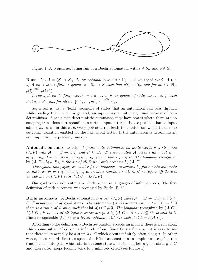
Figure 1: A typical accepting run of a Buchi automaton, with s ∈ Sin and g ∈ G.

Runs Let A = (S,→, Sin) be an automaton and α : N0 → Σ an input word. A runof A on α is a infinite sequence ρ : N0 → S such that ρ(0) ∈ Sin and for all i ∈ N0,

ρ(i)α(i)−→ ρ(i+1).

A run of A on the finite word w = a0a1 . . . am is a sequence of states s0s1 . . . sm+1 such

that s0 ∈ Sin and for all i ∈ {0, 1, . . . , m}, s1α(i)−→ si+1.

So, a run is just a “legal” sequence of states that an automaton can pass throughwhile reading the input. In general, an input may admit many runs because of non-determinism. Since a non-deterministic automaton may have states where there are nooutgoing transitions corresponding to certain input letters, it is also possible that an inputadmits no runs—in this case, every potential run leads to a state from where there is nooutgoing transition enabled for the next input letter. If the automaton is deterministic,each input admits precisely one run.

Automata on finite words A finite state automaton on finite words is a structure(A, F ) with A = (S,→, Sin) and F ⊆ S. The automaton A accepts an input w =a0a1 . . . am if w admits a run s0s1 . . . sm+1 such that sm+1 ∈ F . The language recognizedby (A, F ), L(A, F ), is the set of all finite words accepted by (A, F ).

Throughout this paper, we shall refer to languages recognized by finite state automataon finite words as regular languages. In other words, a set U ⊆ Σ∗ is regular iff there isan automaton (A, F ) such that U = L(A, F ).

Our goal is to study automata which recognize languages of infinite words. The firstdefinition of such automata was proposed by Buchi [Bu60].

Buchi automata A Buchi automaton is a pair (A, G) where A = (S,→, Sin) and G ⊆S. G denotes a set of good states. The automaton (A, G) accepts an input α : N0 → Σ ifthere is a run ρ of A on α such that inf(ρ) ∩G 6= ∅. The language recognized by (A, G),L(A, G), is the set of all infinite words accepted by (A, G). A set L ⊆ Σω is said to beBuchi-recognizable if there is a Buchi automaton (A, G) such that L = L(A, G).

According to the definition, a Buchi automaton accepts an input if there is a run alongwhich some subset of G occurs infinitely often. Since G is a finite set, it is easy to seethat there must actually be a state g ∈ G which occurs infinitely often along σ. In otherwords, if we regard the state space of a Buchi automaton as a graph, an accepting runtraces an infinite path which starts at some state s in Sin, reaches a good state g ∈ Gand, thereafter, keeps looping back to g infinitely often (see Figure 1).

3

����

����

����a b

b

a

s1 s2=⇒

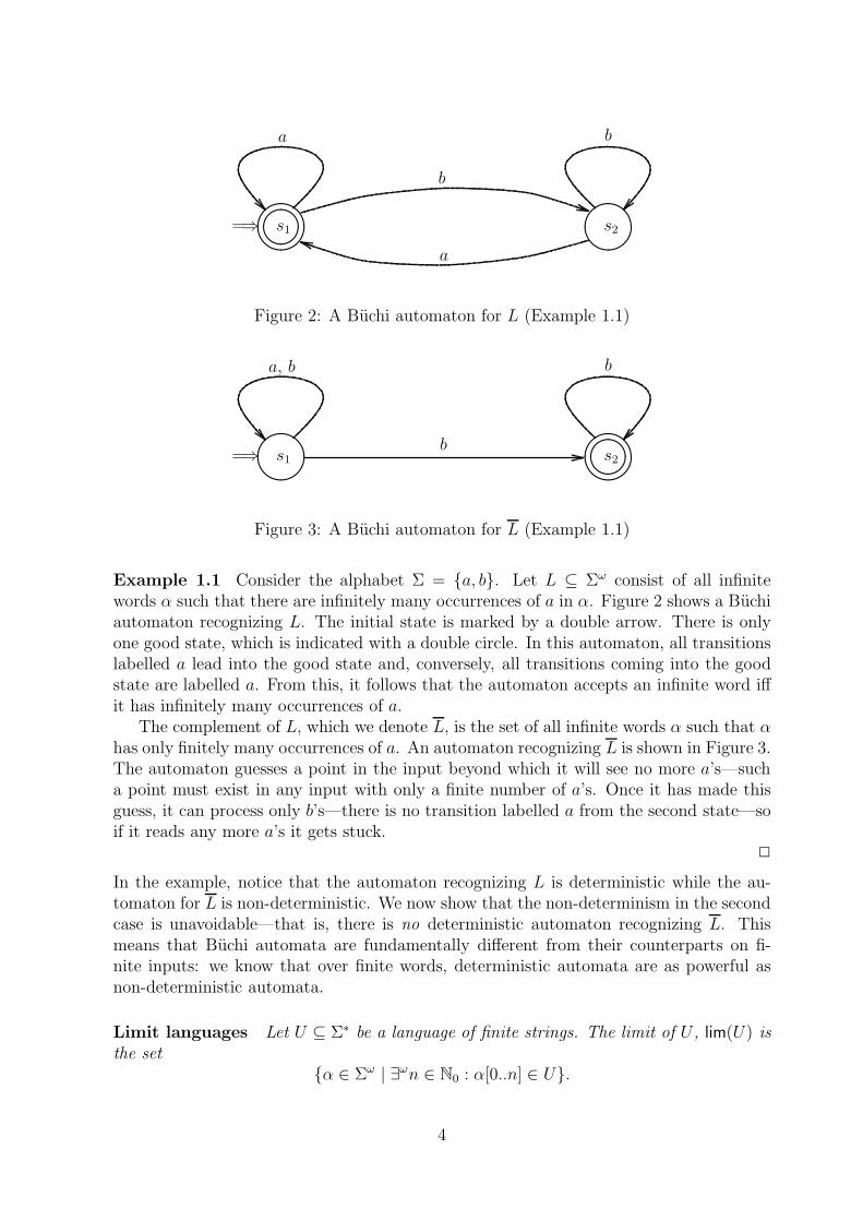
Figure 2: A Buchi automaton for L (Example 1.1)

����

��������b

s1 s2=⇒

a, b

b

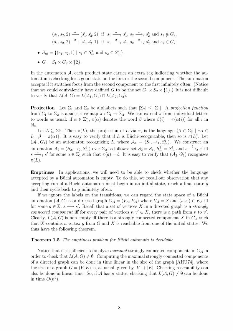
Figure 3: A Buchi automaton for L (Example 1.1)

Example 1.1 Consider the alphabet Σ = {a, b}. Let L ⊆ Σω consist of all infinitewords α such that there are infinitely many occurrences of a in α. Figure 2 shows a Buchiautomaton recognizing L. The initial state is marked by a double arrow. There is onlyone good state, which is indicated with a double circle. In this automaton, all transitionslabelled a lead into the good state and, conversely, all transitions coming into the goodstate are labelled a. From this, it follows that the automaton accepts an infinite word iffit has infinitely many occurrences of a.

The complement of L, which we denote L, is the set of all infinite words α such that αhas only finitely many occurrences of a. An automaton recognizing L is shown in Figure 3.The automaton guesses a point in the input beyond which it will see no more a’s—sucha point must exist in any input with only a finite number of a’s. Once it has made thisguess, it can process only b’s—there is no transition labelled a from the second state—soif it reads any more a’s it gets stuck.

2

In the example, notice that the automaton recognizing L is deterministic while the au-tomaton for L is non-deterministic. We now show that the non-determinism in the secondcase is unavoidable—that is, there is no deterministic automaton recognizing L. Thismeans that Buchi automata are fundamentally different from their counterparts on fi-nite inputs: we know that over finite words, deterministic automata are as powerful asnon-deterministic automata.

Limit languages Let U ⊆ Σ∗ be a language of finite strings. The limit of U , lim(U) isthe set

{α ∈ Σω | ∃ωn ∈ N0 : α[0..n] ∈ U}.

4

So, a word belongs to lim(U) iff it has infinitely many prefixes in U . We then have thefollowing characterization of languages recognized by deterministic Buchi automata.

Theorem 1.2 A language L ⊆ Σω is recognizable by a deterministic Buchi automaton iffL is of the form lim(U) for some regular language U ⊆ Σ∗.

Proof Let U be a regular language. Then, there exists a deterministic finite stateautomaton (DFA) of the form (A, F ) where A = (S,→, Sin) and F ⊆ S such that (A, F )recognizes U . It is easy to see that if we interpret F as a set of good states, the Buchiautomaton (A, F ) accepts lim(U).

Conversely, let L be recognized by a deterministic Buchi automaton (A, G). Treat Gas a set of final states and let U be the language recognized by the DFA (A, G). Onceagain, it is easy to see that L = lim(U). 2

We now show that the language L of Example 1.1 is not of the form lim(U) for anylanguage U . Recall that L is the set of all infinite words α over the alphabet Σ = {a, b}such that α contains only finitely many occurrences of a.

Suppose that L = lim(U) for some U ⊆ Σ∗. Since bω ∈ L, there must be some finiteprefix bn1 ∈ U . Since, bn1abω ∈ L, we can then find a prefix bn1abn2 ∈ U . From thefact that bn1abn2abω ∈ L, we obtain a prefix bn1abn2abn3 ∈ U . Proceeding in this way,we get an infinite sequence of words {bn1 , bn1abn2 , bn1abn2abn3 , . . .} ⊆ U . From this itfollows that the infinite word β = bn1abn2abn3a · · ·abnia · · · belongs to lim(U). But β hasinfinitely many occurrences of a, so it certainly does not belong to L, thus contradictingthe assumption that L = lim(U).

From this observation and Example 1.1, we deduce the following corollary.

Corollary 1.3 Non-deterministic Buchi automata are strictly more powerful than de-terministic Buchi automata—there are languages recognized by non-deterministic Buchiautomata which cannot be recognized by any deterministic Buchi automaton.

1.1 Characterizing Buchi-recognizable languages

For finite words, we can characterize the class of languages recognized by non-deterministicfinite state automata in a number of ways—for instance, in terms of regular expressions, orin terms of syntactic congruences. In the same spirit, we now describe a characterizationof Buchi-recognizable languages of infinite words. We first need to define the ω-iterationof a set of finite words. Let U ⊆ Σ∗. Then

Uω = {α ∈ Σω | α = u0u1u2 · · · where ui ∈ U for all i ∈ N0}.

Also, we observe that if U is a language of finite words and L is a language of infinitewords, we can define the language UL of infinite words obtained by concatenating eachfinite word in U with an infinite word from L. Formally, UL = {α | ∃u ∈ U : ∃β ∈ L :α = uβ}.

5

ω-regular languages A language L ⊆ Σω is said to be ω-regular if it is of the form⋃

i∈{1,2,...,n}UiVωi , where each Ui and Vi is a regular language of finite words.1

Theorem 1.4 A language is Buchi-recognizable iff it is ω-regular.

Proof(⇒):Let L be recognized by a Buchi automaton (A, G), where A = (S,→, Sin). We haveobserved earlier that each infinite word α ∈ L admits an accepting run ρ which begins inan initial state, reaches a good state g, and then loops back through g infinitely often. Fors, s′ ∈ S, let Vss′ = {w ∈ Σ∗ | s

w−→+ s′} denote the set of finite words which can lead from

s to s′. It is easy to see that Vss′ is regular—to recognize this set, use the non-deterministicautomaton (S,→, {s}) with {s′} as the set of final states. From our observation aboutaccepting runs, it follows that we can write L(A, G) as

⋃

s∈Sin, g∈G VsgVωgg.

(⇐):It is not difficult to show that the set of Buchi-recognizable languages satisfies the followingclosure properties:

(i) If U is regular, then Uω is Buchi-recognizable.

(ii) If U is regular and L is Buchi-recognizable then UL is Buchi recognizable.

(iii) If L1, L2, . . . , Ln are Buchi-recognizable, so is⋃

i∈{1,2,...,n} Li.

From this, it follows that every language of the form⋃

i∈{1,2,...,n}UiVωi , where each Ui and

Vi is regular, is Buchi-recognizable. 2

1.2 Constructions on Buchi automata

It turns out that the class of Buchi-recognizable languages is closed under boolean op-erations and projection. These operations will be crucially used when applying Buchiautomata to settle decision problems in logic.

Union To show closure under finite union (which we have already assumed when provingthe previous theorem!), let (A1, G1) and (A2, G2) be two Buchi automata. To constructan automaton (A, G) such that L(A, G) = L(A1, G1) ∪ L(A2, G2), we take A to be thedisjoint union of A1 and A2. Since we are permitted to have a set of initial states inA, we retain the initial states from both copies. If a run of A starts in an initial statecontributed by A1, it will never cross over into the state space contributed by A2 andvice versa. Thus, we can set the good states of A to be the union of the good statescontributed by both components.

1Technically speaking, both regularity and ω-regularity are defined algebraically, in terms of homo-

morphisms from the given language to a finite monoid. However, we shall ignore this complication and

stick to a more simple definition of ω-regularity.

6

Complementation Showing that Buchi-recognizable languages are closed under com-plementation is highly non-trivial. One problem is that we cannot determinize Buchiautomata, as we have observed in Corollary 1.3. Even if we could work with deterministicautomata, the formulation of Buchi acceptance is not symmetric with respect to comple-mentation in the following sense. Suppose (A, G) is a deterministic Buchi automaton andα is an infinite word which does not belong to L(A, G). Then, the (unique) run ρ

αof A

on α is such that inf(ρα) ∩ G = ∅. Let G denote the complement of G. It follows that

inf(ρα)∩G 6= ∅, since some state must occur infinitely often in ρ

α. It would be tempting

to believe that the automaton (A, G) recognizes Σω − L(A, G). However, there may bewords which admit runs which visit both G and G infinitely often. These words will beincluding both in L(A, G) as well as in L(A, G). So, there is no convenient way to expressthe complement of a Buchi condition again as a Buchi condition.

We shall postpone describing a complementation construction for Buchi automatauntil Section 4. Till then we shall, however, assume that we can complement theseautomata.

Intersection Turning to intersection, the natural way to intersect automata A1 and A2

is to construct an automaton whose state space is the cross product of the state spacesof A1 and A2 and let both copies process the input simultaneously. For finite words, theinput is accepted if each copy can generate a run which reaches a final state at the endof the word.

For infinite inputs, we have to do a more sophisticated product construction. Aninfinite input α should be accepted by the product system provided both copies generateruns which visit good states infinitely often. Unfortunately, there is no guarantee thatthese runs will ever visit good states simultaneously—for instance, it could be that thefirst run goes through a good state after α(0), α(2), . . . while the second run enters goodstates after α(1), α(3), . . . So, the main question is one of identifying the good states ofthe product system.

The key observation is that to detect that both components of the product visit goodstates infinitely often, one need not record every point where the copies visit good states;in each copy, it suffices to observe an infinite subsequence of the overall sequence of goodstates. So, we begin by focusing on the first copy and waiting for its run to enter a goodstate. When this happens, we switch attention to the other copy and wait for a goodstate there. Once the second copy reaches a good state, we switch back to the first copyand so on. Clearly, we will switch back and forth infinitely often iff both copies visit theirrespective good states infinitely often. Thus, we can characterize the good states of theproduct in terms of the states where one switches back and forth.

Formally, the construction is as follows. Let (A1, G1) and (A2, G2) be two Buchiautomata such that Ai = (Si,→i, S

iin) for i = 1, 2. Define (A, G), where A = (S,→, Sin),

as follows:

• S = S1 × S2 × {1, 2}

• The transition relation → is defined as follows:

(s1, s2, 1)a

−→ (s′1, s′2, 1) if s1

a−→1 s

′1, s2

a−→2 s

′2 and s1 /∈ G1.

(s1, s2, 1)a

−→ (s′1, s′2, 2) if s1

a−→1 s

′1, s2

a−→2 s

′2 and s1 ∈ G1.

7

(s1, s2, 2)a

−→ (s′1, s′2, 2) if s1

a−→1 s

′1, s2

a−→2 s

′2 and s2 /∈ G2.

(s1, s2, 2)a

−→ (s′1, s′2, 1) if s1

a−→1 s

′1, s2

a−→2 s

′2 and s2 ∈ G2.

• Sin = {(s1, s2, 1) | s1 ∈ S1in and s2 ∈ S2

in}

• G = S1 ×G2 × {2}.

In the automaton A, each product state carries an extra tag indicating whether the au-tomaton is checking for a good state on the first or the second component. The automatonaccepts if it switches focus from the second component to the first infinitely often. (Noticethat we could equivalently have defined G to be the set G1 × S2 ×{1}.) It is not difficultto verify that L(A, G) = L(A1, G1) ∩ L(A2, G2).

Projection Let Σ1 and Σ2 be alphabets such that |Σ2| ≤ |Σ1|. A projection functionfrom Σ1 to Σ2 is a surjective map π : Σ1 → Σ2. We can extend π from individual lettersto words as usual: if α ∈ Σω

1 , π(α) denotes the word β where β(i) = π(α(i)) for all i inN0.

Let L ⊆ Σω1 . Then π(L), the projection of L via π, is the language {β ∈ Σω

2 | ∃α ∈L : β = π(α)}. It is easy to verify that if L is Buchi-recognizable, then so is π(L). Let(A1, G1) be an automaton recognizing L, where A1 = (S1,→1, S

1in). We construct an

automaton A2 = (S2,→2, S2in) over Σ2 as follows: set S2 = S1, S

2in = S1

in and sb

−→2 s′ iff

sa

−→1 s′ for some a ∈ Σ1 such that π(a) = b. It is easy to verify that (A2, G1) recognizes

π(L).

Emptiness In applications, we will need to be able to check whether the languageaccepted by a Buchi automaton is empty. To do this, we recall our observation that anyaccepting run of a Buchi automaton must begin in an initial state, reach a final state gand then cycle back to g infinitely often.

If we ignore the labels on the transitions, we can regard the state space of a Buchiautomaton (A, G) as a directed graph GA = (VA, EA) where VA = S and (s, s′) ∈ EA ifffor some a ∈ Σ, s

a−→ s′. Recall that a set of vertices X in a directed graph is a strongly

connected component iff for every pair of vertices v, v′ ∈ X, there is a path from v to v′.Clearly, L(A, G) is non-empty iff there is a strongly connected component X in GA suchthat X contains a vertex g from G and X is reachable from one of the initial states. Wethus have the following theorem.

Theorem 1.5 The emptiness problem for Buchi automata is decidable.

Notice that it is sufficient to analyze maximal strongly connected components in GA inorder to check that L(A, G) 6= ∅. Computing the maximal strongly connected componentsof a directed graph can be done in time linear in the size of the graph [AHU74], wherethe size of a graph G = (V,E) is, as usual, given by |V |+ |E|. Checking reachability canalso be done in linear time. So, if A has n states, checking that L(A, G) 6= ∅ can be donein time O(n2).

8

2 The logic of sequences

Buchi’s original motivation for studying automata on infinite inputs was to solve a decisionproblem from logic. He discovered a deep and beautiful connection between ω-regularlanguages and sets of models of formulas in certain logics.

S1S

The logic that Buchi considered was the monadic second-order theory of one successor,abbreviated as S1S. This logic is interpreted over the set N0 of natural numbers. Ingeneral, second-order logic permits quantification over relations and functions, unlikefirst-order logic, which permits quantification over just individual variables. However, thefact that we are dealing with a “monadic” second-order logic restricts this extra powerto quantification over one-place relations. Since a one-place relation is just a subset, thiseffectively means that we can quantify over individual elements of N0 and subsets of N0.The fact that we are dealing with “one successor” means we are talking about N0 withthe usual ordering where each element has a unique successor. Permitting two successors,for instance, would produce the infinite binary tree which has countably many nodes buthas two successors for each node.

Formally, the logical language S1S is defined as follows.

Terms A term in S1S is built up from the constant 0 and individual variables x, y, . . .by application of the successor function succ. Thus, the following are terms: 0, succ(x),succ(succ(succ(0))), succ(succ(y)), . . . .

Atomic formulas Let t, t′, . . . be terms. An atomic formula is of the form t = t′ ort ∈ X, where X is a set variable.

Formulas A formula is built up from atomic formulas using the boolean connectives¬ (not) and ∨ (or), together with the existential quantifier ∃. The quantifier ∃ can beapplied to both individual and set variables—one can write ∃x and ∃X. In other words,if ϕ and ψ are inductively assumed to be formulas, so are ¬ϕ, ϕ∨ψ, (∃x) ϕ and (∃X) ϕ.

In addition, we can define the remaining boolean connectives like ∧ (and), ⇒ (if-then),⇔ (iff) as usual, in terms of ¬ and ∨: for instance, ϕ ⇒ ψ is defined as (¬ϕ ∨ ψ). We

also have the universal quantifier ∀ which is the dual of ∃: (∀x) ϕdef= ¬((∃x) ¬ϕ) and

(∀X) ϕdef= ¬((∃X) ¬ϕ).

Assigning truth values to formulas Formulas are interpreted over N0. The con-stant 0 denotes the number 0. Individual variables x, y, . . . are interpreted as naturalnumbers—that is, elements of N0. The function succ corresponds to adding one: succ(x)denotes the number which is one greater than the interpretation of x. Thus, the termsucc(succ(succ(0))) represents the number 3. And, if the current interpretation of x isthe number 47 then succ(x) denotes 48.

The connective = used in defining atomic formulas denotes equality, as usual. Thust = t′ is true provided t and t′ denote the same natural number.

9

Set variables like X, Y , . . . are interpreted as subsets of N0. The atomic formula t ∈ Xis true iff the number denoted by t belongs to the set denoted by X.

Once the interpretation of atomic formulas has been fixed, the meaning of compoundformulas involving ¬, ∨ and ∃ is the “natural” one.

Let ϕ be a formula. A variable is said to occur free in ϕ if it is not within the scope of aquantifier. For instance, in the formula (∃x)(∀Y ) (0 ∈ Y )∨(x = y)∨(x ∈ X), the variablesy and X occur free. Variables which do not occur free are said to be bound. In the pre-ceding formula, x and Y are bound. We write ϕ(x1, x2, . . . , xk, X1, X2, . . . , Xℓ) to indicatethat all the variables which occur free in ϕ come from the set {x1, x2, . . . , xk, X1, X2, . . . , Xℓ}.

Let−→X = (x1, x2, . . . , xk, X1, X2, . . . , Xℓ). To assign a truth value to the formula ϕ(

−→X ), we

have to first fix an interpretation of the variables in−→X . In other words, we must map each

individual variable xi to a natural number mi ∈ N0 and each set variable Xj to a subset

Mj ⊆ N0. Let−→M = (m1, m2, . . . , mk,M1,M2, . . . ,Mℓ). We write

−→M |= ϕ(

−→X ) to denote

that ϕ is true under the interpretation {xi 7→ mi}i∈{1,2,...,k} and {Xi 7→ Mi}i∈{1,2,...,ℓ}.Rather than go into formal details, we look at some illustrative examples.

Example 2.1

(i) Let Sub(X, Y ) = (∀x) x ∈ X ⇒ x ∈ Y .

Then (M,N) |= Sub(X, Y ) iff M ⊆ N .

(ii) Let Zero(X) = (∃x) [x ∈ X ∧ ¬(∃y)(y < x)].

This formula asserts that X contains an element which has no predecessors in N0.Thus, M |= Zero(X) iff 0 ∈M .

(iii) Let Lt(x, y) = (∀Z)[succ(x) ∈ Z ∧ (∀z)(z ∈ Z ⇒ succ(z) ∈ Z)] ⇒ (y ∈ Z).

Then (m,n) |= Lt(x, y) iff m < n. What the formula asserts is that any set Z whichcontains x+1 and is closed with respect to the successor function must also containy.

(iv) Let Sing(X) = (∃Y ) [Sub(Y,X) ∧ (Y 6= X) ∧¬(∃Z) (Sub(Z, Y ) ∧ (Z 6= X) ∧ (Z 6= Y ))].

In this formula, X 6= Y abbreviates ¬(X = Y ), where X = Y is itself an abbrevi-ation for Sub(X, Y ) ∧ Sub(Y,X). The formula asserts that X has only one propersubset, which is Y . This is true only for singletons, where Y is the empty set. So,M |= Sing(X) iff M is a singleton {m}.

2

A sentence is a formula in which no variables occur free. A sentence ϕ is either true orfalse—we do not have to interpret any variables to assign meaning to ϕ. For instanceconsider the sentence

(∀X) [0 ∈ X ∧ (∀x) (x ∈ X ⇒ succ(x) ∈ X)] ⇒ (∀x) x ∈ X.

This sentence is true: it expresses the familiar property of mathematical induction forsubsets of N0—if a set of natural numbers contains 0 and is closed with respect to thesuccessor function, then the set in fact includes all of N0.

10

Satisfiability An S1S formula ϕ(x1, . . . , xk, X1, . . . , Xℓ) is said to be satisfiable if we

can choose−→M = (m1, . . . , mk,M1, . . . ,Mℓ) such that

−→M |= ϕ(

−→X ).

Buchi showed how to associate an ω-regular language Lϕ with each S1S formula ϕ,such that every word in Lϕ represents an interpretation for the free variables in ϕ underwhich the formula ϕ evaluates to true. Moreover, every interpretation which makes ϕ trueis represented by some word in Lϕ. Thus, ϕ is satisfiable iff there is some interpretationwhich makes it true iff Lϕ is non-empty. The language Lϕ is defined over the alphabet{0, 1}m, where m is the number of free variables in ϕ.

In fact, Buchi showed that the converse is also true. Let us say that a languageL ⊆ ({0, 1}m)ω is S1S-definable if L = Lϕ for some S1S formula ϕ. We can always embedan arbitrary alphabet Σ as a subset of {0, 1}m for some suitable choice of m. In this way,any language L ⊆ Σω can be converted into an equivalent language L{0,1} over {0, 1}m.Buchi showed that if L is ω-regular, then L{0,1} is S1S-definable.

Thus, the notions of S1S-definability and ω-regularity are equivalent. The rest of thissection will be devoted to formally stating and proving this result.

We begin by defining Lϕ for an S1S formula ϕ(x1, x2, . . . , xk, X1, X2, . . . , Xℓ). Let−→M = (m1, m2, . . . , mk,M1,M2, . . . ,Mℓ) such that

−→M |= ϕ(

−→X ). We can associate with

−→M an infinite word α

Mover {0, 1}k+ℓ which represents the characteristic function of

−→M .

For i ∈ N0, and j ∈ {1, 2, . . . , k+ℓ}, let αM

(i)(j) denote the jth component of αM

(i).Then for i ∈ N0 and j ∈ {1, 2, . . . , k}, α

M(i)(j) = 1 iff i = mj and α

M(i)(j) = 0 iff

i 6= mj. Similarly, for i ∈ N0, and j ∈ {k+1, k+2, . . . , k+ℓ}, αM

(i)(j) = 1 iff i ∈ Mj andα

M(i)(j) = 0 iff i /∈Mj . Then

Lϕ = {αM|−→M |= ϕ(

−→X )}.

Next we define the {0, 1}-image L{0,1} corresponding to a language L over an arbitraryalphabet Σ. Let Σ = {a1, a2, . . . , am}. Then, each word α ∈ Σω can be represented bya word α{0,1} over {0, 1}m, where for all i ∈ N0 and j ∈ {1, 2, . . . , m}, α{0,1}(i)(j) = 1 ifα(i) = aj and α{0,1}(i)(j) = 0 if α(i) 6= aj. Then

L{0,1} = {α{0,1} | α ∈ L}.

We can now state Buchi’s result more precisely.

Theorem 2.2

(i) Let ϕ be an S1S formula. Then Lϕ is an ω-regular language.

(ii) Let L be an ω-regular language. Then L{0,1} is S1S-definable.2

Proof

(i) To show that Lϕ is ω-regular, we proceed by induction on the structure of ϕ. To dothis, it will be convenient to cut down the language S1S to an equivalent languageS1S0 which has a simpler syntax.

2We have fixed a apecific embedding of Σ into {0, 1}m which is relatively easy to describe in S1S. In

general, we can choose any embedding for defining L{0,1} and the result will still go through.

11

����

����

����s1 s2=⇒

〈1, 0〉

〈0, 0〉〈0, 1〉〈1, 1〉

Figure 4: Buchi automaton for the atomic formula X ⊆ Y

Formally, in S1S0 we do not have individual variables xi—there are only set variablesXj. The atomic formulas are of the form X ⊆ Y and succ(X, Y ). The first formulais true if X is a subset of Y while the second is true if X and Y are singletons {x}and {y} respectively and y = x+1.

We now argue that every S1S formula ϕ can be converted to an S1S0 formula ϕ0

such that Lϕ = Lϕ0.

We begin by eliminating nested applications of the successor function. For instance,if the S1S formula contains the atomic formula succ(succ(x)) ∈ X, we write instead

(∃y)(∃z) y = succ(x) ∧ z = succ(y) ∧ z ∈ X.

We then eliminate formulas of the form 0 ∈ X using the formula Zero(X) definedin Example 2.1.

Finally, we eliminate singleton variables using the formula Sing from Example 2.1.For instance, we rewrite (∀x)(∃y) succ(x) = y ∧ y ∈ Z as

(∀X) (Sing(X) ⇒ [(∃Y ) Sing(Y ) ∧ succ(X, Y ) ∧ Y ⊆ Z]).

Notice that we can uniformly replace Sub(X, Y ) by X ⊆ Y in Sing since X ⊆ Y isan atomic formula in SIS0.

We now construct for each S1S0 formula ϕ, a Buchi automaton (Aϕ, Gϕ) recognizingLϕ.

For the atomic formula X ⊆ Y , the corresponding automaton over {0, 1}×{0, 1} isshown in Figure 4. This automaton accepts any input word which does not contain〈1, 0〉—if α(i) = 〈1, 0〉, in the corresponding interpretation, i ∈ X but i /∈ Y , thusviolating the requirement that X ⊆ Y .

����

����

��������

=⇒

〈0, 0〉 〈0, 0〉

s1 s2 s3〈1, 0〉 〈0, 1〉

Figure 5: Buchi automaton for the atomic formula succ(X, Y )

12

The other atomic formula is succ(X, Y ). The corresponding automaton is shown inFigure 5. This automaton accepts inputs of the form 〈0, 0〉i〈1, 0〉〈0, 1〉〈0, 0〉ω, i ∈ N0,corresponding to the interpretation where X = {i} and Y = {i+1}.

For the induction step, we need to consider the connectives ¬, ∨ and ∃X.

Let ϕ = ¬ψ. Then, Lϕ is the complement of Lψ. By the induction hypothesis,there exists a Buchi automaton (Aψ, Gψ) which recognizes Lψ. As we mentionedearlier, there is an effective way to construct an automaton (Aϕ, Gϕ) recognizingthe complement of Lψ. The details will be described in Section 4.

If ϕ = ϕ1 ∨ ϕ2, then Lϕ = Lϕ1∪ Lϕ2

. By the induction hypothesis, there existautomata (Aϕ1

, Gϕ1) and (Aϕ2

, Gϕ2) such that L(Aϕi

, Gϕi) = Lϕi

for i = 1, 2.We have seen in Section 1.2 how to construct an automaton (Aϕ, Gϕ) such thatL(Aϕ, Gϕ) = Lϕ1

∪ Lϕ2.

Finally, if ϕ = (∃X1) ψ(X1, X2, . . .Xm), the language Lϕ corresponds to the projec-tion of Lψ via the function π : {0, 1}m → {0, 1}m−1 which erases the first componentof eachm-tuple in {0, 1}m. A word of (m−1)-tuples belongs to Lϕ if it can be paddedout with an extra component so that the resulting word over m-tuples is in Lψ. Thispadding operation corresponds to guessing a witness for the set X1. The automaton(Aϕ, Gϕ) recognizing Lϕ can be obtained from (Aψ, Gψ), the automaton recognizingLψ, as described in Section 1.2.

In this way, we inductively associate with each S1S0 formula ϕ, a Buchi automaton(Aϕ, Gϕ) such that Lϕ = L(Aϕ, Gϕ).

There is a slight technicality involved when we deal with sentences. Notice thatevery time we encounter an existential quantifier, we eliminate one component fromthe input alphabet of Aϕ. If ϕ is a sentence—that is, all variables in ϕ are bound—we would have erased all components of the input by the time we construct Aϕ. Inother words, Aϕ will be an input-free automaton whose states and transitions definean unlabelled directed graph. If we were dealing with languages of finite words, wecould say that a sentence ϕ is true iff Lϕ contains the empty word. Since the emptyword is not a member of Σω, we would have to slightly modify our definition of Lϕ toaccommodate this case cleanly in our framework. However, we shall not worry toomuch about this since it is clear that a sentence ϕ is true iff there is an unlabelledpath in the graph corresponding to Aϕ which begins at some initial state and visitsa good state infinitely often.

(ii) Let (A, G) be a Buchi automaton recognizing L ⊆ Σω, where Σ = {a1, a2, . . . , am}and A = (S,→, Sin), with S = {s1, s2, . . . , sk}. We use free variables A1, A2, . . . , Amto describe each infinite word over Σ—the variable Ai describes the positions inthe input where letter ai occurs. We then use existentially quantified variablesS1, S2, . . . , Sk to describe runs of the automaton over the input—the variable Sjdescribes the positions in the run where the automaton is in state sj .

The formula ϕL can then be written as follows:

13

(∃S1)(∃S2) · · · (∃Sk)

(∀x)∨

i∈{1,2,...,m}

(x ∈ Ai) ∧∧

i∈{1,2,...,m}

x ∈ Ai ⇒∨

j 6=i

x /∈ Aj

∧ (∀x)∨

i∈{1,2,...,k}

(x ∈ Si) ∧∧

i∈{1,2,...,k}

x ∈ Si ⇒∨

j 6=i

x /∈ Sj

∧∨

si∈Sin

(0 ∈ Si)

∧ (∀x)∨

(si,aj ,sk)∈→

(x ∈ Si) ∧ (x ∈ Aj) ∧ (succ(x) ∈ Sk)

∧∨

si∈G

(∀x)(∃y) (x < y) ∧ (y ∈ Si)

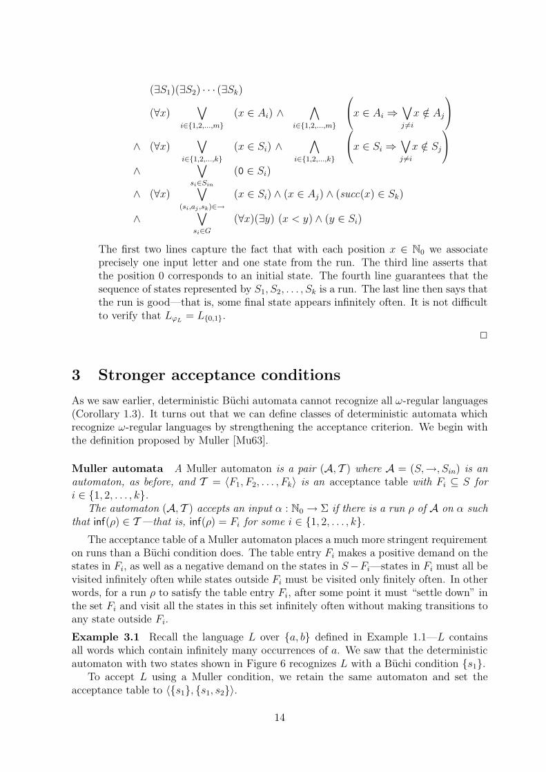
The first two lines capture the fact that with each position x ∈ N0 we associateprecisely one input letter and one state from the run. The third line asserts thatthe position 0 corresponds to an initial state. The fourth line guarantees that thesequence of states represented by S1, S2, . . . , Sk is a run. The last line then says thatthe run is good—that is, some final state appears infinitely often. It is not difficultto verify that LϕL

= L{0,1}.

2

3 Stronger acceptance conditions

As we saw earlier, deterministic Buchi automata cannot recognize all ω-regular languages(Corollary 1.3). It turns out that we can define classes of deterministic automata whichrecognize ω-regular languages by strengthening the acceptance criterion. We begin withthe definition proposed by Muller [Mu63].

Muller automata A Muller automaton is a pair (A, T ) where A = (S,→, Sin) is anautomaton, as before, and T = 〈F1, F2, . . . , Fk〉 is an acceptance table with Fi ⊆ S fori ∈ {1, 2, . . . , k}.

The automaton (A, T ) accepts an input α : N0 → Σ if there is a run ρ of A on α suchthat inf(ρ) ∈ T —that is, inf(ρ) = Fi for some i ∈ {1, 2, . . . , k}.

The acceptance table of a Muller automaton places a much more stringent requirementon runs than a Buchi condition does. The table entry Fi makes a positive demand on thestates in Fi, as well as a negative demand on the states in S−Fi—states in Fi must all bevisited infinitely often while states outside Fi must be visited only finitely often. In otherwords, for a run ρ to satisfy the table entry Fi, after some point it must “settle down” inthe set Fi and visit all the states in this set infinitely often without making transitions toany state outside Fi.

Example 3.1 Recall the language L over {a, b} defined in Example 1.1—L containsall words which contain infinitely many occurrences of a. We saw that the deterministicautomaton with two states shown in Figure 6 recognizes L with a Buchi condition {s1}.

To accept L using a Muller condition, we retain the same automaton and set theacceptance table to 〈{s1}, {s1, s2}〉.

14

����

����

a b

b

a

s1 s2=⇒

Figure 6: Automaton for L and L (Example 3.1)

We also saw that L, the complement of L could not be recognized by any deterministicBuchi automaton. However, it is easy to verify that L can be recognized with a Mullercondition by using the same automaton as for L, but with the acceptance table given by〈{s2}〉. 2

Simulations The example shows that deterministic Muller automata are strictly morepowerful than deterministic Buchi automata. It is quite straightforward to simulate aBuchi automaton by a Muller automaton—we construct an entry in the Muller tablefor each subset of states which contains a good state. Formally, let (A, G) be a Buchiautomaton, where A = (S,→, Sin). The corresponding Muller automaton is given by(A, TG) where TG = {F ⊆ S | F ∩ G 6= ∅}. It is easy to see that L(A, G) = L(A, TG)—any successful run of the Buchi automaton will satisfy one of the entries in the Mullertable. Conversely, any run which satisfies an entry in TG must visit a good state in-finitely often. Notice that the Muller automaton (A, TG) is deterministic iff the originalautomaton (A, G) was deterministic: this simulation neither introduces nor removes anynon-determinism.

Conversely, any Muller automaton can be simulated by a non-deterministic Buchiautomaton. Let (A, T ) be a Muller automaton, where T = 〈F1, F2, . . . , Fk〉. For eachi ∈ {1, 2, . . . , k}, we construct a Buchi automaton (Ai, Gi) such that (Ai, Gi) acceptsan input α iff there is a run ρ of (A, T ) on α with inf(ρ) = Fi. It is easy to see thatL(A, T ) =

⋃

i∈{1,2,...,k}L(Ai, Gi). As described in Section 1.2, we can then construct aBuchi automaton (AT , GT ) which recognizes L(A, T ).

To construct (Ai, Gi) we proceed as follows. When reading an input α, Ai simulates arun of A. At some point, A non-deterministically decides that no more states from S−Fiwill occur along the run being simulated. After this guess is made, Ai will only simulatemoves which stay within Fi. At the same time, Ai repeatedly cycles through Fi, checkingthat all states from Fi are seen infinitely often.

Let A = (S,→, Sin) and Fi = {si1, si2 , . . . , sim}. Then (Ai, Gi), with Ai =(Si,→i, S

iin), is defined as follows:

• Si = {(s, finite) | s ∈ S} ∪ {(s, infinite, j) | s ∈ Fi, j ∈ {0, 1, . . . , m−1}}.

• The transition relation →i is given as follows:

(s, finite)a

−→i (s′, finite) if sa

−→ s′.

15

(s, finite)a

−→i (s′, infinite, 0) if sa

−→ s′ and s′ ∈ Fi.

(s, infinite, k)a

−→i (s′, infinite, k) if sa

−→ s′, s′ ∈ Fi and s 6= sik+1.

(s, infinite, k)a

−→i (s′, infinite, (k+1) mod m) if sa

−→ s′, s′ ∈ Fi and s = sik+1.

• Siin = {(s, finite) | s ∈ Sin}.

• Gi = {(sim , infinite, m−1)}.

These two simulation constructions show that the class of Muller-recognizable languagescoincides with the class of Buchi-recognizable languages. In other words, Muller automataalso recognize ω-regular languages.

However, Example 3.1 suggests that deterministic Muller automata may suffice forrecognizing all ω-regular languages. In fact, this is the case—this non-trivial result wasproved by McNaughton [Mc66].

Theorem 3.2 (McNaughton) Every ω-regular language is recognized by a determinis-tic Muller automaton.

We shall prove McNaughton’s result indirectly in Section 4. Notice that McNaughton’stheorem, combined with the simulation constructions described above, yields a comple-mentation construction for Buchi automata. This is because complementing determin-istic Muller automata is easy. Let (A, T ) be a deterministic Muller automaton, whereA = (S,→, Sin). Let T = {F ⊆ S | F /∈ T }. It is straightforward to verify thatL(A, T ) = Σω −L(A, T ). So, to complement a Buchi automaton (A, G), we first convertit into an equivalent deterministic Muller automaton (A, T ) using McNaughton’s theo-rem. We then simulate (A, T ) using the construction described earlier to get a Buchiautomaton (AT , GT ) which accepts the complement of L(A, G).

Rather than follow this route, we shall describe an alternative determinization con-struction due to Safra [Sa88]. Safra’s construction converts a Buchi automaton to adeterministic automaton with a pairs table. Acceptance in terms of a pairs table firstdescribed by Rabin [Ra69].

Rabin automata A Rabin automaton is a structure (A,PT ) where A = (S,→, Sin)is an automaton, as before, and PT = 〈(G1, R1), (G2, R2), . . . , (Gk, Rk)〉 is a pairs tablewith Gi, Ri ⊆ S for i ∈ {1, 2, . . . , k}.

The automaton (A,PT ) accepts an input α : N0 → Σ if there is a run ρ of A on αsuch that for some i ∈ {1, 2, . . . , k}, inf(ρ) ∩Gi 6= ∅ and inf(ρ) ∩ Ri = ∅.

Thus each pair (Gi, Ri) in the pairs table of a Rabin automaton specifies a positiveand a negative requirement on the run, as in the acceptance table of a Muller automaton.The positive entry Gi is just a Buchi condition while the negative entry Ri is like the onespecified for S−Fi by an entry Fi in a Muller acceptance table. If we think of Gi and Ri

as “green lights” and “red lights”, a run ρ satisfies (Gi, Ri) if some green light from Gi

flashes infinitely often and no red light from Ri flashes infinitely often.Returning to Example 3.1, the language L is accepted by the automaton of Figure 6

with the pairs table 〈({s1}, ∅)〉, while L is accepted by the same automaton with the pairstable 〈({s2}, {s1})〉.

16

Buchi automata can be trivially simulated by Rabin automata—if (A, G) is a Buchiautomaton, the corresponding Rabin automaton is (A,PT G), where PT G = 〈{G, ∅}〉.

Conversely, we can simulate Rabin automata by Buchi automata using a constructionsimilar to the one for simulating Muller automata by Buchi automata. As before, itsuffices to construct a separate Buchi automaton (Ai, G

′i) for each entry (Gi, Ri) in the

pairs table of a Rabin automaton (A,PT ). The automaton (Ai, G′i) simulates a run of

A and guesses when no more states from Ri will be seen. It then checks that states fromGi occur infinitely often.

Let A = (S,→, Sin) and PT = 〈(G1, R1), (G2, R2), . . . , (Gk, Rk)〉. Then (Ai, G′i), with

Ai = (Si,→i, Siin), is defined as follows:

• Si = {(s, finite) | s ∈ S} ∪ {(s, infinite, j) | s ∈ (S − Ri), j ∈ {0, 1}}}.

• The transition relation →i is given as follows:

(s, finite)a

−→i (s′, finite) if sa

−→ s′.

(s, finite)a

−→i (s′, infinite, 0) if sa

−→ s′ and s′ /∈ Ri.

(s, infinite, 0)a

−→i (s′, infinite, 0) if sa

−→ s′, s′ /∈ Ri and s /∈ Gi.

(s, infinite, 0)a

−→i (s′, infinite, 1) if sa

−→ s′, s′ /∈ Ri and s ∈ Gi.

(s, infinite, 1)a

−→i (s′, infinite, 0) if sa

−→ s′ and s′ /∈ Ri.

• Siin = {(s, finite) | s ∈ Sin}.

• G′i = {(s, infinite, 1) | s ∈ (S − Ri)}.

Notice that a Rabin automaton can also simulated by a Muller automaton in quite astraightforward manner. Let (A,PT ) be a Rabin automaton, where A = (S,→, Sin)and PT = 〈(G1, R1), (G2, R2), . . . , (Gk, Rk)〉. Each pair (Gi, Ri) generates a Muller tableTi = {F ⊆ (S − Ri) | F ∩ Gi 6= ∅}. Let T =

⋃

i∈{1,2,...,k} Ti. It is easy to see that(A, T ) recognizes L(A,PT ). Once again, since we have not modified A, the simulatingautomaton is deterministic iff the original automaton was.

To simulate Muller automata using Rabin automata one has to use a constructionwhich is pretty much the same as the one for simulating Muller automata by Buchiautomata. Such a simulation introduces non-determinism: there is no straightforward wayto directly simulate a deterministic Muller automaton by a deterministic Rabin automatoneven though deterministic Rabin automata do recognize all ω-regular languages, as weshall see in the next section.

The last acceptance condition we look at is obtained by interpreting the pairs table ofa Rabin automaton in a complementary fashion.

Streett automata A Streett automaton is a structure (A,PT ) where A = (S,→, Sin)and PT = 〈(G1, R1), (G2, R2), . . . , (Gk, Rk)〉 are defined in the same way as for Rabinautomata.

The Streett automaton (A,PT ) accepts an input α : N0 → Σ if there is a run ρ ofA on α such that for every i ∈ {1, 2, . . . , k}, if inf(ρ) ∩ Gi 6= ∅ it is also the case thatinf(ρ) ∩Ri 6= ∅.

17

These automata were defined by Streett in [St88]. They are useful for describing fairnessconditions in infinite computations—for instance, conditions of the form “if a request fora resource is made infinitely often, then the system grants access to the resource infinitelyoften”. The following observation is immediate from the close connection between Rabinand Streett automata.

Proposition 3.3 Let (A,PT ) be a deterministic automaton with a pairs table. Let LRbe the language accepted by (A,PT ) when PT is interpreted as a Rabin condition and LSbe the language accepted by (A,PT ) when PT is interpreted as a Streett condition. ThenLS is the complement of LR.

As usual, simulating a Buchi automaton (A, G) by a Streett automaton is easy. LetA = (S,→, Sin). Construct an automaton (A,PT G) where PT G = 〈(S,G)〉. Sinceinf(ρ)∩S must be non-empty for any run ρ of A, it follows that a run ρ satisfies the pair(S,G) iff inf(ρ) ∩G 6= ∅, which is precisely what the Buchi condition demands.

In the converse direction, Safra describes a construction due to Vardi which showsthat Streett automata can be efficiently simulated by Buchi automata [Sa88].

Lemma 3.4 Let (A,PT ) be a Street automaton where A = (S,→, Sin). Let n = |S|and let k be the number of pairs in PT : that is, PT = 〈(G1, R1), (G2, R2), . . . , (Gk, Rk)〉.Then, we can construct a Buchi automaton (A′, G′) with A′ = (S ′,→′, S ′

in) such thatL(A′, G′) = L(A,PT ) and |S ′| = n · 2O(k).

Proof The automaton A′ simulates A. As usual, A′ guesses an initial prefix of therun after which every state which is visited by the run will in fact be visited infinitelyoften. After making this guess, A checks that the acceptance criterion is met for eachpair (Gi, Ri) ∈ PT . In other words, for every i such that some state from Gi appears inthe infinite portion of the run, A′ ensures that some state from Ri also appears infinitelyoften. To do this, A′ maintains two sets as part of its state. The first set accumulates thelist of indices corresponding to pairs (Gi, Ri) where some element of Gi occurs infinitelyoften. The second set repeatedly accumulates indices of pairs (Gi, Ri) for which someelement of Ri has been visited. Each time the second set becomes as large as the first, itis reset to empty. It is not difficult to see that the acceptance criterion specified by PTis met iff the second set is reset to empty infinitely often during the simulation.

Formally, we construct (A′, G′) as follows:

• S ′ = {(s, finite) | s ∈ S} ∪ {(s,X1, X2) | s ∈ S and X1, X2 ⊆ {1, 2, . . . , k}}.

• The transition relation →′ is defined as follows:

(s, finite)a

−→′ (s′, finite) if sa

−→ s′.

(s, finite)a

−→′ (s′, ∅, ∅) if sa

−→ s′.

(s,X, Y )a

−→′ (s′, X ∪Gs′, Y ∪ Rs′) if sa

−→ s′ and X ∪Gs′ 6⊆ Y ∪ Rs′,where Gs′ = {i ∈ {1, 2, . . . , k} | s′ ∈ Gi} and

Rs′ = {i ∈ {1, 2, . . . , k} | s′ ∈ Ri}.

(s,X, Y )a

−→′ (s′, X ∪Gs′, ∅) if sa

−→ s′ and X ∪Gs′ ⊆ Y ∪Rs′ .

18

• Siin = {(s, finite) | s ∈ Sin}.

• Gi = {(s,X, ∅) | s ∈ S,X ⊆ {1, 2, . . . , k}}.

2

4 Determinizing Buchi automata

We now describe an elegant construction due to Safra for determinizing Buchi automata[Sa88]. Safra’s construction converts a non-deterministic Buchi automaton (A, G) intoa deterministic Rabin automaton (AG,PT G) such that L(AG,PT G) = L(A, G). If weregard (AG,PT G) as a Streett automaton, we get a deterministic automaton recogniz-ing the complement of L(A, G). By Lemma 3.4, we can simulate the Streett automaton(AG,PT G) by a Buchi automaton. Thus Safra’s construction also solves the complemen-tation problem for Buchi automata.

Also, recall that it is easy to convert a deterministic Rabin automaton into a deter-ministic Muller automaton. As a consequence, Safra’s construction gives an indirect proofof McNaughton’s Theorem (Theorem 3.2).

Safra’s determinization construction for Buchi automata is a clever extension to theinfinite word case of the classical subset construction for determinizing automata on finitewords. In order to motivate the construction, we begin with the subset construction forfinite words and enhance it in a graded manner to achieve the final result.

Subset construction For automata on finite words, the subset construction is thestandard way to eliminate non-determinism. If the original automaton is (A, F ), withA = (S,→, Sin), each state of the subset automaton (Ssub,→sub, S

subin ) is a subset of S.

The (single) initial state of the subset automaton is the set Sin of initial states of A. Thesubset automaton’s transition relation →sub is defined as follows:

Xa

−→sub Y iff Y = {y ∈ S | ∃x ∈ X : xa

−→ y}.

Henceforth, we use δsub(X, a) to denote the set Y such that Xa

−→sub Y .The subset automaton satisfies the following property: If X

w−→+

sub Y then for eachstate y in Y , there is an state x ∈ X such that x

w−→+ y in the original automaton.

From this, it follows that if we set the set of final states of the subset automaton tobe Fsub = {X ⊆ S | S ∩F 6= ∅}, then (Asub, Fsub) recognizes the same set of words as theoriginal automaton.

Let (A, G) be a non-deterministic Buchi automaton, with A = (S,→, Sin). Thenatural extension of the subset construction to Buchi automata would set the good statesof the subset automaton to Gsub = {X ⊆ S | X ∩G 6= ∅}.

It is easy to see that if (A, G) accepts an input α, so will (Asub, Gsub). Unfortunately,the converse is not true—the subset automaton will accept words which are not part ofthe original language.

Example 4.1 Consider the automaton of Example 1.1 (Figure 3) which recognizes Lover {a, b} given by L = {α | α has only a finite number of occurrences of a}.

In this example, Gsub, the set of good states of the extended subset automaton, isgiven by {{s1, s2}, {s2}}. On the input (ab)ω = ababab · · ·, the (unique) run of the subset

19

��

��

��

��

'

&

$

%

��

��

'

&

$

%· · ·a ab b

s1 s1 s1

s2

s1 s1

s2

Figure 7: A run of the extended subset automaton for L on input (ab)ω (Example 4.1)

automaton is {s1}({s1}{s1, s2})ω = {s1}{s1}{s1, s2}{s1}{s1, s2}{s1}{s1, s2} · · ·. Since

this run visits Gsub infinitely often, the automaton (Asub, Gsub) accepts the word (ab)ω,even though a occurs infinitely often in this word.

The problem with the subset construction is best brought out by drawing all the“threads” between the individual subsets in this run of the subset automaton—see Fig-ure 7.

As we can see, every finite run of the original automaton which reaches a good stateactually dies out at that point. In general, all that this subset construction guarantees isthat the original automaton has arbitrarily long finite runs which visit good states. 2

Marked subset construction We next try to strengthen the subset construction sothat it explicitly keeps track of the threads between subsets. In the marked subset con-struction, in addition to keeping a subset of states, the subset automaton also has theability to “mark” each state in the subset. A state in the current subset is marked if itsatisfies one of two conditions: either it is a good state, or it has a marked predecessorin the previous subset. However, if all the states in the previous subset are marked, thenonly good states are marked in the current subset—no marks are inherited from a fullymarked state. The good states in the marked subset automaton are those where the entiresubset is marked.

Concretely, let (A, G) be the original non-deterministic Buchi automaton with A =(S,→, Sin). Then, the marked subset automaton (AM , GM), with AM = (SM ,→M , S

Min ),

is given as follows.

• SM = {(X, f) | X ⊆ S, f : X → {marked, unmarked}}.

• The transition function →M is as follows:

(X, f)a

−→M (Y, g) iff

– Y = δsub(X, a).(Recall that Y = δsub(X, a) iff in the normal subset automaton, X

a−→sub Y .)

– If f(x) = marked for all x ∈ Xthen

∀y ∈ Y : g(y) =

{

marked if y ∈ Gunmarked otherwise

else

∀y ∈ Y : g(y) =

marked if y ∈ G or

(∃x ∈ X : f(x) = marked and xa

−→ y)unmarked otherwise

20

• SMin = {(Sin, f) | ∀s ∈ Sin : f(s) = marked}.

• GM = {(X, f) | ∀x ∈ X : f(x) = marked}.

The main property satisfied by this automaton is the following.

Let ρ be a run of (AM , GM) on an input α such that ρ(i) = (Xi, fi) for alli ∈ Nat. Suppose that (Xk, fk) ∈ G for some k > 0. Let j be the largestnatural number less than k such that (Xj , fj) ∈ G—such a number j mustexist because the initial state of AM belongs to G.

Then, for each state y ∈ Yk, there is a state x ∈ Xj such that x −α[j..k−1]→∗ yin the original automaton and, moreover, when going from x to y on readingα[j..k−1], the original automaton goes through some good state.

From this observation, we can deduce that the marked subset construction is sound.

Proposition 4.2 Let (AM , GM) be the marked subset automaton which corresponds tothe Buchi automaton (A, G). Then, if (AM , GM) accepts an input α, so does (A, G).

Proof Let ρα

be the (unique) run of AM on an input α with ρα(i) = (Xi, fi) for i ∈ N0.

If (AM , GM) accepts α, there must be an infinite sequence of positions {i0, i1, . . .} ⊆ N0

such that 0 = i0 < i1 < · · · and (Xj , fj) ∈ G for all j ∈ {i0, i1, . . .}.From our previous observation about the marked subset construction, we know that

for each index ik+1 in the set {i0, i1, . . .} and for each state x ∈ Xik+1, there is a state

y ∈ Xik such that in the original automaton, there is a sequence of transitions leadingfrom y to x on the input α[ik..ik+1−1] which passes through some good state. Let us callsuch a state y a good predecessor of x.

We construct an infinite tree Tα as follows. The root of the tree is the set Sin of initialstates. At each level k of the tree, k ≥ 1, we have a node n(x,ik) corresponding to eachstate x ∈ Xik . The parent of a node n(x,j) at level j, j > 1, is a node n(y,j−1) at level j−1such y is a good predecessor of x. (Of course, x may have more than one good predecessor.If this is the case, we arbitrarily select one of them and make the corresponding node theparent of n(x,j) in the tree.)

The tree Tα is finitely branching and has an infinite number of nodes. By Konig’slemma, it must have an infinite path. Each infinite path in Tα corresponds to a run ofthe original automaton A on α. By construction, such a run must pass through a goodstate between each level in the tree. Thus, A has at least one run on α which meets Ginfinitely often. 2

Unfortunately, though the marked subset construction is sound, it is not complete—theremay be inputs accepted by (A, G) which are not accepted by (AM , GM). Consider thefollowing example.

Example 4.3In the Buchi automaton shown in Figure 8, the input aω generates the sequence of

subsets {s0}({s1, s2})ω. Since s2 is not a final state, the subset {s1, s2} never becomes

fully marked. Thus, though the original automaton has an accepting run s0sω1 on this

input, the marked subset construction fails to detect this. 2

The problem is that the marked subset construction demands too much from theunderlying runs. As the example shows, it should be sufficient to identify a portion of thesubset which is marked and which can infinitely often regenerate its marks.

21

���� ��

��

��������

((((((((((

hhhhhhhhhh

s0

s1

s2

a

a

a

a

=⇒

Figure 8: The marked subset construction is not complete (Example 4.3)

Hierarchical Marked Subset Construction A first attempt to weaken the markedsubset construction would be to have a hierarchy of marks. At the base level, the subsetautomaton runs the marked subset construction and marks states using a level 1 mark.The states which have level 1 marks then start off a nested copy of the marked subsetconstruction with level 2 marks. Similarly, the states which have level 2 marks start off amarked subset construction with level 3 marks. What we would like to detect is whethersome level i can get completely marked. This corresponds to checking if the set of nodesmarked at level i is equal to the set of nodes marked at level i+1. If so, we reset all marksat levels greater than i and continue.

Since the number of nodes marked at level i is always strictly greater than the set ofnodes marked at level i+1, there can be at most as many levels as there are states in theoriginal automaton.

To specify the acceptance condition, we need to verify that some level i+1 gets setto empty infinitely often and that level i does not get set to empty in between. In otherwords, level i denotes a permanent thread through the subset construction which getsmarked infinitely often. To do this, we have to pass from a Buchi condition to a Rabincondition—for each i, a positive condition for level i+1 has to be qualified by a negativecondition for level i.

Here is a formal description of a hierarchical marked subset construction which at-tempts to achieve this goal. Let (A, G) be a Buchi automaton, with A = (S,→, Sin).Define (AH ,PT H), with AH = (SH ,→H, S

Hin), as follows:

• Let |S| = n. SH consists of pairs of the form (σ, χ) where:

– σ : {1, 2, . . . , n} → 2S is a subset list satisfying the condition that σ(i+1) is aproper subset of σ(i) whenever σ(i) is non-empty.

– χ : {1, 2, . . . , n} → {white, green} is a colour list.

• SHin = (σ0, χ0), where σ0(1) = Sin, σ0(i) = ∅ for all i ∈ {2, 3, . . . , n} and χ(i) = white

for all i ∈ {1, 2, . . . , n}.

• The transition function →H performs the following sequence of actions. Initially,each level runs the subset construction locally. Next, any final states appearing inthe new subset at level i are added to the subset at level i+1—this corresponds togenerating fresh marks at level i. We now look for the smallest level i whose subset

22

is the same as that at level i+1. If such an i exists, we “clear out” the subset listfrom level i+1 onwards and set the colour of level i to green.

More formally, on reading an input a, the state (σ, χ) generates a new state (σ′, χ′)as follows:

(i) Let σ1 : {1, 2, . . . , n+ 1} → 2S be defined as follows:

– σ1(1) = δsub(σ(1), a).

– For i ∈ {2, 3, . . . , n}, σ1(i) = δsub(σ(i), a) ∪ (δsub(σ(i−1), a) ∩G).

– σ1(n+1) = δsub(σ(n), a) ∩G.

(ii) If there is no index i ∈ {1, 2, . . . , n} such that σ1(i) = σ1(i+1), then

– σ′(i) = σ1(i) for all i ∈ {1, 2, . . . , n}.

– χ′(i) = white for all i ∈ {1, 2, . . . , n}.

else, let m be the smallest index such that σ1(m) = σ1(m+1). Then,

– σ′(i) = σ1(i) for all i ∈ {1, 2, . . . , m} and σ′(i) = ∅ for all i > m.

– χ′(m) = green and χ′(i) = white for all i 6= m.

• The acceptance table PT H consists of n pairs 〈(G1, R1), (G2, R2), . . . , (Gn, Rn)〉where:

– Ri = {(σ, χ) | σ(i) = ∅}

– Gi = {(σ, χ) | χ(i) = green}

In this construction, the list σ implicitly records the levels of marks associated with thestates in the current subset—a state s belongs to σ(i+1) iff s has a level i mark in thecurrent subset. It is not difficult to show that this construction is complete.

Proposition 4.4 Let (AH ,PT H) be the hierarchical marked subset automaton whichcorresponds to the Buchi automaton (A, G). If (A, G) accepts an input α, so does(AH ,PT H).

Proof Suppose (A, G) accepts α. Then, α admits a run ρ which visits G infinitely often.We must show that the unique run ρ

αof AH on α satisfies some entry in PT H .

For j ∈ N0, let ρα(j) = (σj , χj). We know that for all j ∈ N0, σj(1) is the set of states

maintained by the subset construction. Since ρ is a valid run of A on α, σj(1) is alwaysnon-empty. So, ρ

αsatisfies condition R1. If it also satisfies G1 then (AH ,PT H) accepts

α and we are done.If ρ

αdoes not satisfy G1, let k0 be the last position where the colour of the first level

is green. We wait for the first position i0 > k0 where ρ, the accepting run of A on α,next visits a good state. We know that σj(2) is non-empty for all j ≥ i0—once the goodstate seen at position i0 gets pushed to level 2, the accepting run ρ will be part of thesubset construction maintained at level 2, thus guaranteeing that at least one valid stateis generated at each point. So, ρ

αsatisfies R2. If it also satisfies G2 we are done.

Otherwise, we repeat the argument above and deduce that ρα

satisfies R3, with theaccepting run ρ a part of σj(3) for all j greater than a finite index i1. We can repeat this

23

��������

����

����

����

PPPPPPPPPPPP

!!!!!!!!!AAAAAAA

g1

=⇒

a, b

g2

b

a

a

b

s

Figure 9: The hierarchical marked subset construction is not sound (Example 4.5)

argument only a finite number of times, till we reach level n. The subset maintained atlevel n can never be more than a singleton. If the accepting run ρ is part of the subsetconstruction at level n, it must generate the signal green infinitely often in which case ρ

α

satisfies the pair (Gn, Rn). 2

Unfortunately, the hierarchical subset construction is not sound. Consider this exam-ple.

Example 4.5The automaton shown in Figure 9 does not accept the input (ba)ω. However, the run

of the hierarchical marked subset automaton on this input is the following:

1 ({s},white)2 (∅,white)3 (∅,white)

b−→H

1 ({s, g1},white)2 ({g1},white)3 (∅,white)

a−→H

1 ({s, g2},white)2 ({g2}, green)3 (∅,white)

b−→H

1 ({s, g1, g2},white)2 ({g1, g2},white)3 ({g2},white)

a−→H

1 ({s, g2},white)2 ({g2}, green)3 (∅,white)

b−→H · · ·

Since level 2 remains populated forever and turns green infinitely often, the hierarchicalconstruction incorrectly accepts this input. 2

In the preceding example, the problem is that the good state g2 which appears to bepermanently part of level 2 is actually a transient state. Each time an a is read, the g2

state at level 2 disappears, only to be replaced by a fresh copy of g2 which is pushed fromlevel 1.

To rectify this defect, Safra’s construction maintains each level of marks as a disjointset of nodes. The hierarchy of subsets then becomes a tree, with the set at level 1 as theroot.

Safra’s Construction Before presenting Safra’s construction, we review some termi-nology regarding trees. A tree is a structure T = (V, vr, π) where V is a set of nodes,vr ∈ T is a special node known as the root and for all v ∈ V − {vr}, π(v) ∈ T fixes the

24

parent of the node. If v = πi(v′) for some i > 0, we say that v is an ancestor of v′. Theroot vr is an ancestor of every other node. If v′ = π(v) then v is said to be a child of v′.We assume that for any node v, all the children of v are ordered so that we can talk ofone child being to the left of another. This generates a total order on nodes—if v and v′

are nodes, we say that v < v′ if v is an ancestor of v′ or if there is a common ancestoru of v and v′ such that v is in the subtree rooted at a child u1 of v, v′ is in the subtreerooted at a child u2 of v and u1 is to the left of u2.

Given a Buchi automaton (A, G), with A = (S,→, Sin), Safra’s construction producesa Rabin automaton (AG,PT G), with AG = (SG,→G, S

Gin). The automaton (AG,PT G) is

as follows:

• Each state in SG is a structure (T, σ, χ, λ) where

– T = (V, vr, π) is a tree.

– σ : V → 2S associates a set of states of A with each node in V in such a waythat:

∗ The union of the sets associated with the children of a node v is a propersubset of σ(v).

∗ If v and v′ are two nodes such that v is not an ancestor of v′ and v′ is notan ancestor of v then σ(v) is disjoint from σ(v′).

∗ If σ(v) = ∅, then v is the root vr.

It is not difficult to verify that the conditions imposed on the function σ ensurethat |V | can be no larger than n, where n is the number of states in S.

– χ : V → {white, green} fixes a colour for each node.

– λ : V → L is an injective function which attaches a label from the set L ={ℓ1, ℓ2, . . . , ℓ2n} to each node. Notice that L has 2n elements.

• On reading an input a, the state (T, σ, χ, λ) is transformed to the state (T ′, σ′, χ′, λ′)as follows:

(i) Let T = (V, vr, π). Expand the T to a tree T1 = (V1, vr, π1) as follows: Foreach v ∈ V , if σ(v) ∩ G 6= ∅, add a node v′ such that π1(v

′) = v and v′ is theright-most child of v.

(ii) Extend σ and λ to functions σ1 and λ1 over T1 as follows:

For all nodes v in V1 ∩ V , let σ1(v) = σ(v). For a new node v ∈ V1 − V ,σ1(v) = σ(π1(v)) ∩G.

All nodes v in V1 ∩V inherit the label λ(v). For each node in V1 −V , choose anew label from L which is not assigned to any other node. Since there 2n labelsto choose from, this is always possible—each node in V generates at most onenew child in V1 and there were not more than n nodes in V .

(iii) For every node v, apply the subset construction locally. In other words, definea new function σ′

1 : V1 → 2S such that σ′1(v) = δsub(σ1(v), a) for all v ∈ V1.

At this stage, we have to “clean up” T1 and σ′1 so that the structure once again

satisfies the conditions specified for states of AG.

25

(iv) For every node v ∈ V1, if s ∈ σ′1(v) and s also belongs to σ′

1(v′) for some smaller

node v′, v′ < v, (recall the total order on all nodes in a tree) remove s fromσ′

1(v).

(v) Remove all nodes v such that σ′1(v) = ∅ and v is not the root vr.

(vi) For each node v such that σ′1(v) is equal to

⋃

{σ′1(v

′) | v = π1(v′)}, remove all

the children of v and set χ1(v) = green. For all other nodes, set χ1(v) = white.

(vii) Let the set of nodes remaining be V ′. For v ∈ V ′, σ′(v) is that part of σ′1(v)

which remains after discarding states which already appear to the left, as spec-ified in step (iv) above. The label λ′(v) of a node v is retained from T1. Finally,set χ′ = χ1.

• The initial state of AG is the tree ({vr}, vr, ∅) where σ(vr) = Sin, χ(vr) = white andλ(vr) = ℓ1.

• The pairs table PT G = 〈(G1, R1), (G2, R2), . . . , (G2n, R2n)〉 is defined as follows:

– Ri = {(T = (V, vr, π), σ, χ, λ) | ∀v ∈ V : λ(v) 6= ℓi}.

– Gi = {(T = (V, vr, π), σ, χ, λ) | ∃v ∈ V : λ(v) = ℓi and χ(v) = green}.

The labelling procedure guarantees that the labels of new nodes added at each stage aredisjoint from the labels of the existing nodes. In other words, if a node labelled ℓi isdeleted from the tree during a transition, the label ℓi temporarily disappears from thetree.

Thus, an entry (Gi, Ri) in the pairs table specifies the following condition. The condi-tion Ri is satisfied if at some stage a node labelled ℓi is added to the tree and it is neverdeleted henceforth. The condition Gi then says that this node turns green infinitely often.

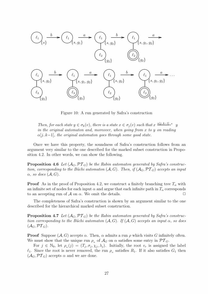
Figure 10 describes the run generated by Safra’s construction on the input (ba)ω forthe automaton shown in Figure 9. In the figure, each node of a tree is denoted by a circle,with the label indicated inside the circle and the associated subset written by its side.Nodes coloured green are drawn as double circles, while white nodes are drawn as singlecircles. When selecting labels for new nodes added to the tree at each stage, we havefollowed the policy of using the first “free” label in L.

At the second level of the tree, nodes labelled ℓ2 and ℓ3 turn green infinitely often,so the run satisfies G2 and G3. However, since both these labels also disappear from thetree infinitely often, the run does not satisfy R2 or R3, thus ensuring that the automatonrejects this input.

It is not difficult to see that Safra’s construction satisfies a property similar to theonly described for the marked subset construction:

Let ρ be a run of (AG,PT G) on an input α such that ρ(i) = (Ti, σi, χi, λi) forall i ∈ N0. Let j, k ∈ N0 with j < k and ℓ be a label from L such that:

• For all positions i ∈ {j, j+1, . . . , k}, there is a node v in the tree Ti suchthat λi(v) = ℓ.

• χj(v) = χk(v) = green and for all i such that j < i < k, χi(v) = white.

26

��������

��������

����

��������

����

��������

����

��������

��������

����

����

ℓ1

ℓ3

{g2}

ℓ1

ℓ3{g2}

ℓ1

ℓ2

ℓ1

ℓ2

b ba a· · ·

ℓ1{s}

ℓ1b

{s, g1}ℓ1

ℓ2

ℓ1

ℓ2{g2}

a b a

{s, g2} {s, g1, g2}{s, g2}

{g2} {g2}

{s, g1, g2}

{g2}

{s, g2} {s, g1, g2}

Figure 10: A run generated by Safra’s construction

Then, for each state y ∈ σk(v), there is a state x ∈ σj(v) such that x −α[j..k−1]→∗ yin the original automaton and, moreover, when going from x to y on readingα[j..k−1], the original automaton goes through some good state.

Once we have this property, the soundness of Safra’s construction follows from anargument very similar to the one described for the marked subset construction in Propo-sition 4.2. In other words, we can show the following.

Proposition 4.6 Let (AG,PT G) be the Rabin automaton generated by Safra’s construc-tion, corresponding to the Buchi automaton (A, G). Then, if (AG,PT G) accepts an inputα, so does (A, G).

Proof As in the proof of Proposition 4.2, we construct a finitely branching tree Tα withan infinite set of nodes for each input α and argue that each infinite path in Tα correspondsto an accepting run of A on α. We omit the details. 2

The completeness of Safra’s construction is shown by an argument similar to the onedescribed for the hierarchical marked subset construction.

Proposition 4.7 Let (AG,PT G) be the Rabin automaton generated by Safra’s construc-tion corresponding to the Buchi automaton (A, G). If (A, G) accepts an input α, so does(AG,PT G).

Proof Suppose (A, G) accepts α. Then, α admits a run ρ which visits G infinitely often.We must show that the unique run ρ

αof AG on α satisfies some entry in PT G.

For j ∈ N0, let ρα(j) = (Tj , σj, χj , λj). Initially, the root vr is assigned the label

ℓ1. Since the root is never removed, the run ρα

satisfies R1. If it also satisfies G1 then(AG,PT G) accepts α and we are done.

27

If ρα

does not satisfy G1, let k1 be the last position at which the root is coloured green.Let i1 be the first position after k where ρ, the accepting run of A on α, visits G. At thispoint, a child v1 of the root comes into existence.

We know that the accepting run ρ is part of the overall subset construction maintainedby the root node. Once v1 is created, we know that ρ is also being maintained at thefirst level. It would appear that the run is maintained by v1 itself, but there is a subtlecomplication to be taken into account. Since we only retain the left-most copy of eachstate, the run ρ may be passed on by v1 to some sibling on the left. In any case, it canonly move left a finite number of times. Let us suppose it eventually settles down at somenode v′1.

It is not difficult to verify that the node v′1 must already have been in the tree whenv1 was added. Let ℓi1 = λi1(v

′1) be the label of v′1. Since α never dies out, v′1 will never

be deleted from the tree. In other words, ρα

satisfies the condition Ri1 . If it satisfies thecorresponding condition Gi1 we are done.

Otherwise, let k2 be the last time where v′1 turns green. As before, we wait for i2, thenext time ρ visits a good state, and look at the child v2 of v′1 which is created at thispoint. The run ρ is copied into the subset maintained by v2 and passed on left a finitenumber of times till it settles down at a node v′2. If ℓi2 is the label of v′2, ρα

must satisfyRi2 . If ρ

αdoes not also satisfy Gi2 we push ρ down one more level.

Since there are only n levels in the tree, we cannot do this indefinitely. Thus, we musteventually find a node v′m labelled ℓim such that ρ

αsatisfies the pair (Gim , Rim). 2

The complexity of Safra’s construction The automaton AG has 2O(n logn) states,where n is the number of states in A. To see this, we estimate the number of bits requiredto write down a typical state of AG. We have to specify the structure (T, σ, λ, χ).

Since T has at most n nodes, we can “name” the nodes {1, 2, . . . , n}, with vr = 1. Thestructure (V, vr, π) can then be written down as a list of the form {π(i)}i∈{1,2,...,n}. Sinceπ(i) ∈ {1, 2, . . . , n} requires logn bits to write down, T can be described using n lognbits. Similarly, λ and χ can be written as lists of length n with each entry made up oflogn bits and 1 bit, respectively.

The only catch is with σ—if we naıvely represent the function σ : V → 2S as a list ofsubsets, we will need n bits to represent each entry, resulting in n2 bits overall. However,notice that if a state s belongs to σ(v) and σ(v′) for two different nodes v and v′ it mustbe the case that v is an ancestor of v′ or that v′ is an ancestor of v. Also, if s ∈ σ(v), smust belong to σ(v′) for every ancestor v′ of v, all the way upto the root. Thus, we cancharacterize the set of nodes where s appears in terms of the lowest node vs such thats ∈ σ(vs): if s ∈ σ(vs) then s ∈ σ(v′) for any other node v′ iff v′ is an ancestor of vs. Inthis way, σ can also be represented as a list of length n by matching each state s in S toits corresponding node vs in V . Each entry in this list can be written down using log nbits.

Since we can characterize a state of AG using O(n logn) bits, it follows that the numberof distinct states is bounded by 2O(n logn).

The number of pairs in PT G is O(n)—by construction, there is a pair (Gi, Ri) for eachlabel ℓi ∈ L and L contains exactly 2n elements.

By Lemma 3.4, we can simulate the Streett automaton (AG,PT G) by a Buchi automa-ton with 2O(n logn) states. Thus, complementing Buchi automata using Safra’s construction

28

results in the state space blowing up from n to 2O(n logn). Recall that for automata onfinite words, the number of states in the complement (via the subset construction) is 2O(n).It has been shown that the bound achieved by Safra’s construction is optimal [Mi88].

Why complement Buchi automata? We have seen that if we work with Muller,Rabin or Streett conditions, we can in fact accept all ω-regular languages using deter-ministic automata. So, why do we bother about complementing non-deterministic Buchiautomata?

The reason is that the natural translation of logical questions into automata necessarilyintroduces non-determinism. For instance, when we constructed the automaton (Aϕ, Gϕ)corresponding to an S1S formula ϕ in Section 2, non-determinism was unavoidable inthe inductive step for handling existential quantification. This non-determinism arisesregardless of what type of acceptance condition we choose to work with. Surprisingly,determinizing Muller or Rabin automata directly is no easier than first converting themto Buchi automata and then applying Safra’s construction [Sa88].

Arguably, for our purposes it should suffice to complement Buchi automata— deter-minization is a stronger construction which yields complementation as a corollary. In fact,Klarlund [Kl91] has shown that it is possible to directly complement non-deterministicBuchi automata without determinizing them and without sacrificing the optimal 2O(n logn)

bound achieved by Safra’s construction. However, there are applications where deter-minization is crucial—for instance, in the game-theoretic analysis of automata on infinitetrees [GH82].

5 Discussion

Our main focus in this survey has been in describing how Buchi automata can be used tosettle decision problems in logic. On the way, we have proved some simple results aboutω-regular languages. There has also been a lot of work on the algebraic and topologicalaspects of ω-regular languages which we have not even touched on. A detailed introductioncan be found in the survey [Th90].

As mentioned in the Introduction, Meyer showed in [Me75] that the decision procedurefor S1S has a non-elementary complexity. A formula of length n may generate an automa-

ton with 22···2

states, where the tower of exponentials is of height n. In other words, thesize of the automaton cannot be bounded by a function of constant exponential height.This result appears to make it impossible to use this elegant theory in a practical settingfor verifying properties of programs.

However, for temporal logics, it turns out that there are direct ways to construct aBuchi automaton (Aϕ, Gϕ) recognizing Lϕ for a temporal logic formula ϕ, such that thesize of Aϕ is exponential in the length of the formula [VW86]. As shown in [VW86],Buchi automata also provide a clean solution to the model-checking problem for finitestate systems. The model checking problem is the following—given a finite-state programP and a temporal logic formula ϕ, do all the computations of P satisfy ϕ?

Rabin showed that Buchi’s decidability result for S1S could be extended to the logicS2S, the monadic second order theory of the infinite binary tree [Ra69]. The logic S2S isvery powerful—for instance, it is powerful enough to embed the logic SωS, the monadicsecond order theory of the infinite countably branching tree.

29

Rabin’s results are proved by extending the techniques developed for automata oninfinite words to automata operating on infinite trees. These extensions are highly non-trivial—especially the result that automata on infinite trees are closed under complemen-tation. A number of attempts have been made to simplify Rabin’s difficult proof. Anovel and fruitful approach has been to analyze these automata in terms of infinite games[GH82].

Recently, there has been a lot of work on lifting the theory of Buchi automata and ω-regular languages to the setting of concurrent programs [GP92, EM93]. When dealing withconcurrent programs, it is often advantageous to regard the runs of the system as partialorders rather than as sequences. Two actions in such a run are unordered if they occurindependently. A sequential description of a concurrent program will generate a number ofequivalent interleavings for each partially ordered run. To verify properties of a concurrentprogram in terms of such a sequential description, we have to check all these equivalentinterleavings when, in principle, it should suffice to check one representative interleavingfor each partially ordered computation. By directly working with infinite labelled partialorders rather than infinite sequences, we can avoid some of this duplication of effort. Achallenging open problem is to extend the work of [GP92, EM93] to branching structureswith concurrency, corresponding to the case of infinite trees for sequential systems.

Acknowledgments I thank Deepak D’Souza, P. Madhusudan, Samik Sengupta andBarbara Sprick for patiently listening to me when I lectured on this material. Theirquestions and observations in class have greatly influenced the manner in which I haveorganized the material in this tutorial. In particular, Example 4.5 is due to Madhu andBarbara.

References

[AHU74] A.V. Aho, J.E. Hopcroft and J.D. Ullman: The Design and Analysisof Algorithms, Addison-Wesley, Reading (1974).

[Bu60] J.R. Buchi: On a decision method in restricted second order arithmetic, Z.Math. Logik Grundlag. Math, 6 (1960) 66–92

[EM93] W. Ebinger and A. Muscholl: Logical Definability on Infinite Traces,Proc. ICALP ’93, LNCS 700 (1993) 335–346.

[Em90] E.A. Emerson: Temporal and modal logic, in: J. van Leeuwen ed., Hand-book of Theoretical Computer Science: Volume B , North-Holland, Amsterdam(1990) 995–1072.

[GP92] P. Gastin and A. Petit: Asynchronous Cellular Automata for InfiniteTraces, Proc. ICALP ’92, LNCS 623 (1992) 583–594.

[GH82] Y. Gurevich and L. Harrington: Trees, automata and games, Proc 14thACM STOC, (1982) 60–65.

[Kl91] N. Klarlund: Progress measures for complementation of ω-automata withapplications to temporal logic, Proc. 32nd IEEE FOCS (1991) 358–367.

30

[Mc66] R. McNaughton: Testing and generating infinite sequences by a finite au-tomaton, Inform. Control, 9 (1966) 521–530.

[Me75] A. Meyer: Weak monadic second order theory of successor is not elementaryrecursive, Proc. Logic Colloquium, Lecture Notes in Mathematics 453 (1975)132–154.

[Mi88] M. Michel: Complementation is more difficult with automata on infinitewords, Manuscript (1988).

[Mu63] D.E. Muller: Infinite sequences an finite machines, Proc. 4th IEEE Symp.on Switching Circuit Theory and Logical Design, (1963) 3–16.

[Pn77] A. Pnueli: The temporal logic of programs, Proc. 18th IEEE FOCS (1977)46–57.

[Ra69] M.O. Rabin: Decidability of second order theories and automata on infinitetrees, Trans. AMS, 141(1969) 1–37.

[Sa88] S. Safra: On the complexity of ω-automata, Proc. 29th IEEE FOCS, (1988)319–327.

[SV89] S. Safra and M. Vardi: On ω-automata and temporal logic, Proc. 21stACM STOC, (1989) 127–137.

[SVW87] A.P. Sistla, M. Vardi and P. Wolper: The complementation problemfor ω-automata with applications to temporal logic, Theoret. Comput. Sci.,49 (1987) 217–237.

[St88] R. Streett: Propositional dynamic logic of looping and converse is elemen-tarily decidable, Inform. Control, 48 (1981) 261–283.

[Th90] W. Thomas: Automata on infinite objects, in J. van Leeuwen (ed.), Hand-book of Theoretical Computer Science, Volume B, North-Holland, Amsterdam(1990) 133–191.

[VW86] M. Vardi and P. Wolper: An automata theoretic approach to automaticprogram verification, Proc. 1st IEEE LICS, (1986) 332–345.

[VW94] M. Vardi and P. Wolper: Reasoning about infinite computations, Inform.Comput., 115(1) (1994) 1–37.

31