infinite color urn models
TRANSCRIPT

Infinite Color Urn Models
Debleena Thacker
Indian Statistical Institute
August, 2014
Revised: April, 2015.


Infinite Color Urn Models
Debleena Thacker
Thesis Supervisor: Antar Bandyopadhyay
Thesis submitted to the Indian Statistical Institute
in partial fulfillment of the requirements
for the award of the degree of
Doctor of Philosophy
August, 2014
Revised: April, 2015
Indian Statistical Institute
7, S.J.S. Sansanwal Marg, New Delhi, India.


Acknowledgments
I thank the faculty and the administrative staff of Indian Statistical Institute, New Delhi,
where I am affiliated as a graduate student, and carried out most of the research work available
in this thesis. I also thank the Theoretical Statistics and Mathematics Unit of Indian Statistical
Institute, Kolkata, where I am presently visiting.
This thesis in its current form, would have been impossible without the perennial support
and supervision of my thesis advisor, Antar Bandyopadhyay. I sincerely thank him for his
encouragements, thoughtful guidance, critical comments and corrections of the thesis. It has
been a pleasure and an honor to work with him.
I am truly grateful to the teachers of Indian Statistical Institute, New Delhi who taught
me. Special thanks to Abhay G. Bhatt, Rahul Roy, Arijit Chakrabarty, Anish Sarkar, Antar
Bandyopadhyay, Arup Pal and Rajendra Bhatia for the many basic and advanced level courses
that they offered.
I am highly indebted to Rahul Roy of Indian Statistical Institute, New Delhi, who has
constantly inspired and appreciated me in all my endeavors. This thesis would have never
materialized without his encouragement.
I am also grateful to Krishanu Maulik of Indian Statistical Institute, Kolkata. He gave useful
insights of research and suggested several valuable corrections in the first draft of one of my
papers.
I am grateful to Codina Cotar of University College, London, for being a wonderful mentor.
She provided timely advice on several crucial career oriented decisions.
Campus life in Indian Statistical Institute, New Delhi has been a memorable affair with
several friends, with whom I shared true moments of pure joy and unadulterated pleasure. Though
it is impossible to thank everyone individually here, I will express a few words of gratitude
to those who have been very close to me. First and foremost, my sincerest gratitude goes to
Farkhondeh Sajadi, who has been a wonderfully supportive friend through moments of crisis.
i

I thank Kumarjit Saha for providing me with useful advice. I specially thank Neha Hooda for
being a great friend, with whom I share many unforgettable memories. Another person with
whom I share a special bond of friendship is Pooja Soni. I cherish the memories that I have
with Neha and Pooja. I am highly indebted to Akansha Batra for her wonderful tips on several
occasions. I thank Sourav Ghosh for being a friend, with whom I could discuss novels and
fictions. I am grateful to Rahul Saha, Indranil Sahoo and Mohana Dasgupta for being wonderful
friends. I also thank Gursharn Kaur for being a wonderful colleague and a good friend.
Finally, I would like to pay deepest gratitude to my family and close friends. I especially
thank my mother, who always had unwavering faith and confidence in me. She is and will always
be my greatest friend and confidant. My deepest gratitude to Tamal Banerjee, to whom I always
turn to in moments of need.
I thank the anonymous referees for their helpful comments, remarks and suggestions. These
have significantly improved the quality of the thesis.
Debleena Thacker
August, 2014,
Revised: April, 2015.
ii

Contents
1 Introduction 1
1.1 Model description . . . . . . . . . . . . . . . . . . . . . . . . . . . . . . . . . 2
1.1.1 Urn models with infinitely many colors . . . . . . . . . . . . . . . . . 3
1.2 Motivation . . . . . . . . . . . . . . . . . . . . . . . . . . . . . . . . . . . . . 4
1.2.1 A simple but useful example . . . . . . . . . . . . . . . . . . . . . . . 6
1.3 Outline and brief sketch of the results . . . . . . . . . . . . . . . . . . . . . . 9
1.3.1 Central limit theorems for the urn models associated with random walks 9
1.3.2 Local limit theorems for the urn models associated with random walks . 9
1.3.3 Large deviation principle for the urn models associated with random walks 9
1.3.4 Representation theorem . . . . . . . . . . . . . . . . . . . . . . . . . 10
1.3.5 General replacement matrices . . . . . . . . . . . . . . . . . . . . . . 10
1.4 Notations . . . . . . . . . . . . . . . . . . . . . . . . . . . . . . . . . . . . . 10
2 Central limit theorems for the urn models associated with random walks 13
2.1 Central limit theorem for the expected configuration . . . . . . . . . . . . . . . 15
2.2 Weak convergence of the random configuration . . . . . . . . . . . . . . . . . 19
2.3 Rate of convergence of the central limit theorem: the Berry-Essen bound . . . . 26
2.3.1 Berry-Essen Bound for d = 1 . . . . . . . . . . . . . . . . . . . . . . 26
2.3.2 Berry-Essen bound for d ≥ 2 . . . . . . . . . . . . . . . . . . . . . . . 29
2.4 Urns with Colors Indexed by other lattices on Rd . . . . . . . . . . . . . . . . 31
3 Local limit theorems for the urn models associated with random walks 35
3.1 Local limit theorems for the expected configuration . . . . . . . . . . . . . . . 35
iii

3.1.1 Local limit theorems for one dimension . . . . . . . . . . . . . . . . . 36
3.1.2 Local limit theorems for higher dimensions . . . . . . . . . . . . . . . 45
4 Large deviation principle for the urn models associated with random walks 55
4.1 Large deviation principle for the randomly selected color . . . . . . . . . . . . 56
5 Representation theorem 61
5.1 Representation theorem . . . . . . . . . . . . . . . . . . . . . . . . . . . . . . 61
5.2 Color count statistics . . . . . . . . . . . . . . . . . . . . . . . . . . . . . . . 64
5.3 Applications of the representation theorem for finite color urn models . . . . . 67
5.3.1 Irreducible and aperiodic replacement matrices . . . . . . . . . . . . . 67
5.3.2 Reducible replacement matrices . . . . . . . . . . . . . . . . . . . . . 70
6 General replacement matrices 73
6.1 Infinite color urn models with irreducible and aperiodic replacement matrices . 73
6.2 Urn models associated with random walks on Zd . . . . . . . . . . . . . . . . 84
6.3 Urn models associated with bounded increment periodic random walk . . . . . 88
Bibliography 93
iv

Chapter 1
Introduction
In recent years, there has been a wide variety of work on random reinforcement models of
various kinds [26, 55, 47, 41, 5, 34, 48, 54, 14, 22, 25, 23, 44, 20, 17]. Urn models form an
important class of random reinforcement models, with numerous applications in engineering
and informatics [60, 42, 50] and bioscience [19, 30, 31, 5, 44]. In recent years there have been
several works on different kinds of urn models and their generalizations [41, 5, 34, 14, 25, 23,
45, 20, 44, 17]. For occupancy urn models, where one considers recursive addition of balls into
finite or infinite number of boxes, there are some works which introduce models with infinitely
many colors, typically represented by the boxes [29, 37, 39].
As observed in [51], the earliest mentions of urn models are in the post-Renaissance period
in the works of Huygen, de Moivre, Laplace and other noted mathematicians and scientists. The
rigorous study of urn models began with the seminal work of Polya [57, 56], where he introduced
the model to study the spread of infectious diseases. We will refer to this model as the classical
Polya urn model. Since then, various types of urn schemes with finitely many colors have been
widely studied in literature [36, 35, 3, 4, 53, 38, 40, 41, 5, 34, 14, 15, 25, 18, 17]. See [54] for
an extensive survey of the known results. However, other than the classical work by Blackwell
and MacQueen [13], there has not been much development of infinite color generalization of the
Polya urn scheme. In this thesis, we introduce and analyze a new Polya type urn scheme with
countably infinite number of colors.
1

2 Chapter 1: Introduction
1.1 Model description
A generalized Polya urn model with finitely many colors can be described as follows:
Consider an urn containing finitely many balls of different colors. At any time
n ≥ 1, a ball is selected uniformly at random from the urn, the color of the selected
ball is noted, the selected ball is returned to the urn along with a set of balls of
various colors which may depend on the color of the selected ball.
The goal is to study the asymptotic properties of the configuration of the urn. Suppose there
are K ≥ 1, different colors and we denote the configuration of the urn at time n by Un =
(Un,1, Un,2 . . . , Un,K), where Un,j denotes the number of balls of color j, 1 ≤ j ≤ K. The
dynamics of the urn model depend on the replacement policy. The replacement policy can be
described by a K ×K matrix, say R with non negative entries. The (i, j)-th entry of R is the
number of balls of color j which are to be added to the urn if the selected color is i. In literature,
R is termed as the replacement matrix. Let Zn denote the random color of the ball selected at
the (n+ 1)-th draw. The dynamics of the model can then be written as
Un+1 = Un +RZn (1.1.1)
where RZn is the Zn-th row of the replacement matrix R.
A replacement matrix is said to be balanced, if the row sums are constant. In this case,
after every draw a constant number of balls are added to the urn. For such an urn, a standard
technique is to divide each entry of the replacement matrix by the constant row sum, thus
without loss of generality, one may assume that the row sums are all 1, that is, the replacement
matrix is a stochastic matrix. In that case, it is also customary to assume U0 to be a probability
distribution on the set of colors, which is to be interpreted as the probability distribution of
the selected color of the first ball drawn from the urn. Note that, in this case the entries of
Un = (Un,1, Un,2 . . . , Un,K) are no longer the number of balls of different colors, instead the
entries of Un/ (n+ 1) are the proportion of balls of different colors. We will refer to it as the
(random) configuration of the urn. It is useful to note here that the random probability mass

1.1 Model description 3
function Un/ (n+ 1) represents the probability distribution of the random color of the (n+ 1)-th
selected ball given the n-th configuration of the urn. In other words, if Zn is the color of the ball
selected at the (n+ 1)-th draw, then,
P(Zn = i
∣∣∣U0, U1, . . . , Un
)=
Un,in+ 1
, 1 ≤ i ≤ K. (1.1.2)
Since R is a stochastic matrix and U0 a probability distribution on the set of colors, we can
now consider a Markov chain on the set of colors with transition matrix R and initial distribution
U0. We call such a chain, a chain associated with the urn model and vice-versa. In other words,
given a balanced urn model we can associate with it a Markov chain on the set of colors and
conversely, given a Markov chain there is an associated urn model with colors indexed by the
state space.
1.1.1 Urn models with infinitely many colors
The above formulation can now be easily generalized for infinitely many colors. Let the colors
be indexed by a finite or countably infinite set S, and the replacement matrix R, be a stochastic
matrix suitably indexed by S. Let Un := (Un,v)v∈S ∈ [0,∞)S , where Un,v is the weight of the
v-th color in the urn after n-th draw. In other words,
P(
(n+ 1)−th selected ball has color v∣∣∣Un, Un−1, · · · , U0
)∝ Un,v, v ∈ S. (1.1.3)
Starting withU0 as a probability vector, the dynamics of (Un)n≥0 is defined through the following
recursion
Un+1 = Un + χn+1R (1.1.4)
where χn+1 = (χn+1,v)v∈S is such that χn+1,Zn = 1 and χn+1,u = 0 if u 6= Zn, where Zn is
the random color chosen from the configuration Un. In other words,
Un+1 = Un +RZn
where RZn is the Zn−th row of the matrix R.
It is important to note here that in general Un,v is not necessarily an integer. When S is

4 Chapter 1: Introduction
infinite, Un,v can be made an integer after suitable multiplication only for certain restrictive cases.
One such case is when each row of R is finitely supported with all entries rational. However,
as discussed in Section 1.1, Un/ (n+ 1) will always denote the proportion of balls of various
colors.
When S is infinite we will call such a process an urn model with infinitely many colors.
The associated Markov chain is on the state space S, with transition probability matrix R and
initial distribution U0. As observed in the finite color case, in general, the random probability
mass function Un/ (n+ 1) represents the probability distribution of the random color of the
(n+ 1)-th selected ball given the n-th configuration of the urn. Recall that Zn denotes the
(n+ 1)-th selected color. Thus for any v ∈ S,
P(Zn = v
∣∣∣Un, Un−1, · · · , U0
)=
Un,vn+ 1
, (1.1.5)
which implies
P (Zn = v) =E [Un,v]
n+ 1. (1.1.6)
In other words, the distribution of Zn is given by the expected proportion of the colors at time n.
It is worthwhile to note here, (1.1.3) and (1.1.4) imply that(Unn+1
)n≥0
is a time inhomogeneous
Markov chain with state space as the set of all probability measures on S.
It is to be noted here, that we write all vectors as row vectors, unless otherwise stated.
1.2 Motivation
Our main motivations to study such a process have been twofold. It is known in the literature
[38, 40, 14, 15, 25], that the asymptotic properties of a finite color urn depend on the qualitative
properties of the underlying Markov chain. For example, for an irreducible aperiodic chain with
K colors, it is shown in [38, 40] that, as n→∞,
Un,jn+ 1
−→ πj a.s. (1.2.1)

1.2 Motivation 5
for all 1 ≤ j ≤ K, where π = (πj)1≤j≤K is the unique stationary distribution of the associated
Markov chain. It is also known [40, 41] that if the chain is reducible and j is a transient state
then, as n→∞,Un,jn+ 1
−→ 0 a.s. (1.2.2)
Further non-trivial scalings have been derived for the reducible case [40, 41, 14, 15, 25]. So one
may conclude that asymptotic properties of an urn model depend on the recurrence/transience of
the underlying states. We want to investigate this relation when there are infinitely many colors.
In [7], we studied the infinite color model, with colors indexed by Zd, where R is the transition
matrix of a bounded increment random walk on Zd. The bounded increment random walks on
Zd, is a rich class of examples of Markov chains on infinite states covering both the transient and
null recurrent cases. Needless to state, that for the finite color case, the associated Markov chain
can posses no null recurrent state. As we shall see later, our study will indicate a significantly
different phenomenon for the infinite color urn models associated with the bounded increment
random walks on Zd. In fact, we shall show that the asymptotic configuration is approximately
Gaussian, irrespective of whether the underlying walk is transient or recurrent.
Another motivation comes from the work of Blackwell and MacQueen [13], where the
authors introduced a possibly infinite color generalization of the Polya urn scheme. In fact, their
generalization even allowed uncountably many colors; the set of colors typically taken as some
Polish space. The model then describes a process whose limiting distribution is the Ferguson
distribution [12, 13], also known as the Dirichlet process prior in the Bayesian statistics literature
[33]. The replacement mechanism in [13] is a simple diagonal scheme, that is, it reinforces only
the chosen color. As in the classical finite color Polya urn scheme, where R is the identity matrix,
this leads to exchangeable sequence of colors. We complement the work of [13], by considering
replacement mechanisms with non-zero off-diagonal entries. We would like to point out that
due to the presence of off-diagonal entries in the replacement matrix, our models do not exhibit
exchangeability and hence the techniques used to study our model are entirely different and new.
We will present a coupling of the urn model with the associated Markov chain, which will be our
most effective method in analyzing the urn models introduced in this work.

6 Chapter 1: Introduction
1.2.1 A simple but useful example
We present a simple example to motivate the study of urn models with infinitely many colors.
Let the colors be indexed by N ∪ {0}, and U0 = δ0. The replacement matrix R is given by
R(i, j) =
1 if j = i+ 1 for all i, j ∈ N ∪ {0},
0 otherwise.(1.2.3)
Note that R has non-zero off diagonal entries. Since R is given by (1.2.3), after every draw a
new color is introduced with positive probability. Hence, even though the urn contains only
finitely many colors after every draw, we require to index the set of colors by the infinite set
N ∪ {0}, to define the process.
The associated Markov chain (Xn)n≥0 on the state space N ∪ {0}, with transition matrix R
given by (1.2.3), is a deterministic chain always moving one step to the right. Therefore, we call
this Markov chain the right shift and the corresponding urn process (Un)n≥0 as the urn model
associated with the right shift. Note that, the right shift is trivially a transient chain.
Theorem 1.2.1. Consider an urn model (Un)n≥0 associated with the right shift, such that theprocess starts with a single ball of color 0. If Zn denotes the (n+ 1)-th selected color then, asn→∞,
Zn − log n√log n
⇒ N(0, 1). (1.2.4)
To prove Theorem 1.2.1 we use the following lemma.
Lemma 1.2.1. Let (Ij)j≥1 be a sequence of independent Bernoulli random variables withE [Ij ] = 1
j+1 , j ≥ 1. If τn =∑n
j=1 Ij , and τ0 ≡ 0, then as n→∞,
τn − log n√log n
⇒ N (0, 1) . (1.2.5)
Proof. E [τn] =∑n
j=1 E [Ij ] =∑n
j=11j+1 . Therefore,
E [τn] ∼ log n, as n→∞, (1.2.6)
where for any two sequences (an)n≥1 and (bn)n≥1 of positive real numbers, we write an ∼ bnto denote lim
n→∞
anbn
= 1.

1.2 Motivation 7
Similar calculations show that
s2n = Var (τn) =
∑nj=1
1j+1 −
1(j+1)2
∼ log n, as n→∞. (1.2.7)
Since Ij can possibly take only two values, namely 0, and 1, so for any ε > 0, we have
1
s2n
n∑j=1
E[∣∣∣Ij − 1
j + 1
∣∣∣21{|Ij− 1j+1|>εsn}
]−→ 0, as n→∞.
Therefore, the Lindeberg-Feller Central Limit theorem (see page 129 of [28]) implies that asn→∞,
τn − E [τn]√log n
⇒ N (0, 1) , (1.2.8)
since the variance of τn is given by (1.2.7). Observe that,
τn − log n√log n
=τn − E [τn]√
log n+
E [τn]− log n√log n
.
It is easy to see that E [τn]− log n =∑n
j=11j+1 − log n −→ γ − 1, as n→∞, where γ is the
Euler’s constant (see page 192 of [2]). Therefore, from (1.2.8) and Slutsky’s theorem (see page105 of [28]), we get as n→∞,
τn − log n√log n
⇒ N (0, 1) . (1.2.9)
Proof of Theorem (1.2.1). As observed earlier in (1.1.6), we know that
P (Zn = v) =E [Un,v]
n+ 1. (1.2.10)
Therefore, the moment generating function E[eλZn
]for Zn is given by
1
n+ 1
∑j∈N∪{0}
E [Un,j ] eλj , for λ ∈ R. (1.2.11)
For every λ ∈ R, let x (λ) =(eλj)Tj∈N∪{0}. It is easy to see that eλ and x (λ) satisfy
Rx (λ) = eλx (λ) ,

8 Chapter 1: Introduction
where the equality holds coordiante-wise. Define the vector scalar product
Unx (λ) =∑
j∈N∪{0}
Un,jeλj . (1.2.12)
From (1.1.4) and (1.1.6), we know that
E[χn∣∣Un−1
]=Un−1
n.
Therefore, it follows that
E[Unx (λ)
∣∣Un−1
]=
(1 +
eλ
n
)Un−1x (λ) .
This implies,
1
n+ 1E [Unx (λ)] =
1
n+ 1
∑j∈N∪{0}
E [Un,j ] eλj =
1
n+ 1
(1 +
eλ
n
)E [Un−1]x (λ) .
Repeating the same iteration, we obtain
1
n+ 1E [Unx (λ)] =
1
n+ 1
n∏j=1
(1 +
eλ
j
)
=n+1∏j=1
(1− 1
j + 1+
eλ
j + 1
). (1.2.13)
Observe that the right hand side of (1.2.13) gives the moment generating function of τn, where τnis as in Lemma 1.2.1. Note that τn is a non-negative random variable for every n ≥ 0. Therefore,from Theorem 1 on page 430 of [32] it follows that for all n ≥ 0,
Znd= τn, (1.2.14)
where for any two random variables X and Y , the notation X d= Y denotes that X and Y have
the same distribution. Hence (1.2.5) implies (1.2.4). This completes the proof.
Later, in Chapters 2 and 5, we will further improve the representation (1.2.14) for urn models
with general replacement matrices. This representation is new and will serve as the key tool in
deriving the asymptotic properties of the urns with more general replacement matrices.

1.3 Outline and brief sketch of the results 9
1.3 Outline and brief sketch of the results
The rest of this work is broadly divided into five chapters. The first three chapters, Chapters 2,
3 and 4 discuss the various asymptotic properties of the urn models associated with bounded
increment random walks on Zd. Chapters 5 and 6 consider urn models with general replacement
matrices.
1.3.1 Central limit theorems for the urn models associated with random walks
Based on [7] and [8], in Chapter 2, we study an urn process when S = Zd, and R is the transition
matrix of a bounded increment random walk on Zd. This is a novel generalization of the Polya
urn scheme, which combines perhaps the two most classical models in probability theory, namely
the urn model and the random walk. We prove central limit theorems for the random color of the
n-th selected ball and show that, irrespective of the null recurrent or transient behavior of the
underlying random walks, the asymptotic distribution is Gaussian after appropriate centering
and scaling. In fact, we show that the order of any non-zero centering is always O (log n) and
the scaling is O(√
log n). In this chapter, we also prove Berry-Essen type bounds and show that
the rate of convergence of the central limit theorem is of the order O(
1√logn
).
1.3.2 Local limit theorems for the urn models associated with random walks
In Chapter 3, we further consider urn models associated with bounded increment random walks
on Zd. In this chapter, we obtain finer asymptotes for the distribution of the randomly selected
color. We derive the local limit theorems for the probability mass function of the randomly
selected color, [7].
1.3.3 Large deviation principle for the urn models associated with random walks
Based on [8], in Chapter 4, we study further asymptotic properties of urn models associated with
bounded increment random walks on Zd. Here, we show that for the expected configuration a
large deviation principle (LDP) holds with a good rate function and speed log n. Moreover, we
prove that the rate function is the same as the rate function for the large deviation of the random
10 Chapter 1: Introduction
walk sampled at random stopping times, where the stopping times follow Poisson distribution
with mean 1.
1.3.4 Representation theorem
In Chapter 5 we consider general urn models. Here S may be any countable set and the
replacement matrix R is any stochastic matrix suitably indexed by S. For this model, we present
a representation theorem (see Theorem 5.1.1), [6]. This theorem provides a coupling of the
marginal distribution of the randomly selected color with the associated Markov chain, sampled
at independent, but random times. We show some immediate applications of the representation
theorem by rederiving a few known results for finite color urn models.
1.3.5 General replacement matrices
In Chapter 6, based on [6], we consider urn models with infinite but countably many colors and
general replacement matrices. In this chapter, we consider several different types of general
replacement matrices and apply the representation theorem to deduce the asymptotic properties
of the corresponding urn models. In Section 6.1, we consider an urn model with an irreducible,
aperiodic R. If R is positive recurrent, with a stationary distribution π, then we show that the
distribution of the randomly selected color converges to π. In Sections 6.2 and 6.3, we further
generalize the model studied in Chapter 2. Here, we study urn models associated with general
random walks, not necessarily with bounded increments, and derive the central limit theorem for
the randomly selected color.
1.4 Notations
We mostly follow notations and conventions that are standard in the literature of urn models. For
the sake of completeness, we provide a list below.
• As mentioned earlier, for any two sequences (an)n≥1 and (bn)n≥1 of positive real numbers,
we will write an ∼ bn, if limn→∞
anbn
= 1.

1.4 Notations 11
• As mentioned earlier, all vectors are written as row vectors, unless otherwise stated. For
x ∈ Rd, we write x =(x(1), x(2), . . . , x(d)
)where x(i) denotes the ith coordinate. The
infinite dimensional vectors are written as y = (yj)j∈J where yj is the jth coordinate and
J is the indexing set. To be consistent, column vectors are denoted by xT , where x is a
row vector.
• For any vector x, x2 will denote a vector with the coordinates squared. That is, if
x = (xj)j∈J for some indexing set J , then
x2 =(x2j
)j∈J .
• The inner product of any two row vectors x and y is denoted by 〈x, y〉.
• The symbol Id will denote the d× d identity matrix.
• ByNd (µ,Σ) we denote the d-dimensional Gaussian distribution with mean vector µ ∈ Rd,
and variance-covariance matrix Σ. For d = 1, we simply write N(µ, σ2), where σ2 > 0.
• The standard Gaussian measure on Rd will be denoted by Φd. Its density φd is given by
φd (x) :=1
(2π)d/2e−‖x‖2
2 , x ∈ Rd.
For d = 1, we will simply write Φ for the standard Gaussian measure on R and φ for its
density.
• The symbol⇒ will denote weak convergence of probability measures.
• The symbolp−→ will denote convergence in probability.
• For any two random variables/vectors X and Y , we will write X d= Y , to denote that X
and Y have the same distribution.

12 Chapter 1: Introduction

Chapter 2
Central limit theorems for the urnmodels associated with random walks1
The main focus in this chapter is to study the urn models associated with bounded increment
random walks on Zd, d ≥ 1. Urn models associated with more general random walks are
discussed in Section 6.2 of Chapter 6. Here, we derive the central limit theorems for the
randomly selected colors, and its rate of convergence. In Section 2.4, we will further generalize
the model when the associated random walk takes values in general d-dimensional discrete
lattices.
Let (Yj)j≥1 be i.i.d. random vectors taking values in Zd with probability mass function
p (u) := P (Y1 = u) , u ∈ Zd. We assume that the distribution of Y1 is bounded, that is there
exists a non-empty finite subset B ⊂ Zd, such that p (u) = 0 for all u 6∈ B. We shall always
write
µ := E [Y1]
Σ = ((σij))1≤i,j≤d := E[Y T
1 Y1
]e (λ) := E
[e〈λ,Y1〉
], λ ∈ Rd.
(2.0.1)
It is easy to see that Σ is a positive semi definite matrix, that is, for all a ∈ Rd,
aΣaT = E[(aY T
1
)2] ≥ 0.
1This chapter is based on the papers entitled “Polya Urn Schemes with Infinitely Many Colors” [7] and “ Rateof Convergence and Large Deviation for the Infinite Color Polya Urn Schemes” [8]. The paper [8] is published inStatistics and Probability Letters, Vol. 92, 2014.
13

14 Chapter 2: Central limit theorems for the urn models associated with random walks
Observe that
Σ = D + µµT ,
where D is the the variance-covariance matrix of Y1.
In this chapter, we assume that Σ is positive definite. This will hold, if and only if, the set B
contains d linearly independent vectors. Later, in Section 6.2 we will relax the assumption that
Σ is positive definite. The matrix Σ1/2 will denote the unique positive definite square root of Σ,
that is, Σ1/2 is a positive definite matrix such that Σ = Σ1/2Σ1/2. When the dimension d = 1,
we will denote the mean and second moment (and not the variance) of Y1 simply by µ and σ2
respectively, that is
µ := E [Y1]
σ2 := E[Y 2
1
].
(2.0.2)
In that case we assume σ2 > 0.
Let Sn := Y0 + Y1 + · · · + Yn, n ≥ 0, be the random walk on Zd starting at Y0 and with
increments (Yj)j≥1 which are independent. Needless to say, that (Sn)n≥0 is a Markov chain,
with initial distribution given by the distribution of Y0 and the transition matrix
R := ((p (v − u)))u,v∈Zd . (2.0.3)
For the rest of this chapter, we consider the urn process (Un)n≥0, with replacement matrix
given by (2.0.3). Since the associated Markov chain is a random walk, we will call the urn
process as the urn process associated with a bounded increment random walk. The urn model
associated with the right shift as discussed in Subsection 1.2.1 of Chapter 1, is an example of an
urn model associated with a bounded increment random walk, which as discussed earlier, is a
deterministic walk always moving one step to the right.
We would like to note here that this model is a further generalization of a subclass of models
studied in [20], namely the class of linearly reinforced models. In [20], the authors prove that
for such models the number of balls of each color grows to infinity. As we will see in the next
section, our results will not only show that the number of balls of each color grows to infinity,
but will also provide the exact rates of their growths.

2.1 Central limit theorem for the expected configuration 15
2.1 Central limit theorem for the expected configuration
We present in this subsection the central limit theorem for the randomly selected color, [7]. The
centering and scaling of the central limit theorem (Theorem 2.1.1) are of the order O (log n)
and O(√
log n)
respectively. Such centering and scalings are available because the marginal
distribution of the randomly selected color behaves like that of a delayed random walk, where
the delay is of the order O (log n), see Theorem 2.1.2.
For simplicity, in Sections 2.1 and 2.2 we will assume that the initial configuration of the
urn consists of a single ball of color 0, that is, U0 = δ0. We will see at the end of Section 2.2
(Remark 2.2.1) that this assumption can be easily removed.
Theorem 2.1.1. Let Λn be the probability measure on Rd corresponding to the probabilityvector
(E[Un,v ]n+1
)v∈Zd
, and let
Λcsn (A) := Λn
(√log nAΣ1/2 + µ log n
),
where A is a Borel subset of Rd. Then, as n→∞,
Λcsn ⇒ Φd. (2.1.1)
If Zn denotes the (n+ 1)-th selected color then, its probability mass function is given by(E[Un,v ]n+1
)v∈Zd
. Thus Λn is the probability distribution of Zn, and Λcsn is the distribution of the
scaled and centered random vector Zn−µ logn√logn
. So the following result is a restatement of (2.1.1).
Corollary 2.1.1. Consider the urn model associated with the random walk (Sn)n≥0 on Zd, d ≥1, then as n→∞,
Zn − µ log n√log n
⇒ Nd(0, Σ). (2.1.2)
We begin by constructing a martingale which we will be need in the proof of Theorem 2.1.1.
Define Πn (z) =n∏j=1
(1 +
z
j
)for z ∈ C. It is known from Euler product formula for
gamma function, which is also referred to as Gauss’ formula (see page 178 of [21]), that
limn→∞
Πn(z)
nzΓ(z + 1) = 1, (2.1.3)
16 Chapter 2: Central limit theorems for the urn models associated with random walks
where the convergence is uniform on compact subsets of C \ {−1,−2, . . .}.
Recall for every λ ∈ Rd, e (λ) :=∑
v∈B e〈λ,v〉p(v) is the moment generating function of
Y1. Define x (λ) :=(e〈λ,v〉
)Tv∈Zd . It is easy to see that
Rx (λ) = e (λ)x (λ) ,
where the equality holds coordinate-wise.
Let Fn = σ (Uj : 0 ≤ j ≤ n) , n ≥ 0, be the natural filtration. Define
Mn (λ) :=Unx (λ)
Πn (e (λ)).
From the fundamental recursion (1.1.4), we get,
Un+1x (λ) = Unx (λ) + χn+1Rx (λ) .
Thus,
E[Un+1x (λ)
∣∣∣Fn] = Unx (λ) + e (λ)E[χn+1x (λ)
∣∣∣Fn] =(
1 + e(λ)n+1
)Unx (λ) .
Therefore, Mn (λ) is a non-negative martingale for every λ ∈ Rd. In particular, E[Mn (λ)
]=
M0 (λ). We now present a representation of the marginal distribution of Zn, in terms of the
increments (Yj)j≥1, where the distribution of Yj is given by p (·) for every j ≥ 1.
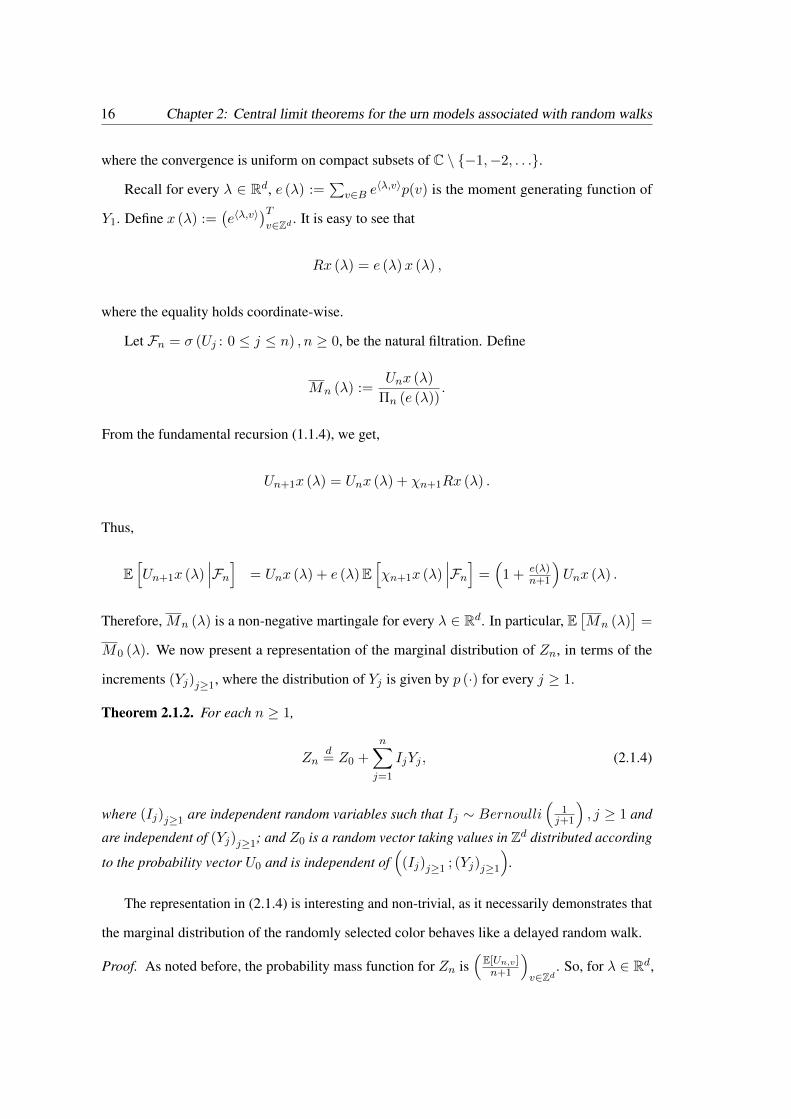
Theorem 2.1.2. For each n ≥ 1,
Znd= Z0 +
n∑j=1
IjYj , (2.1.4)
where (Ij)j≥1 are independent random variables such that Ij ∼ Bernoulli(
1j+1
), j ≥ 1 and
are independent of (Yj)j≥1; and Z0 is a random vector taking values in Zd distributed according
to the probability vector U0 and is independent of(
(Ij)j≥1 ; (Yj)j≥1
).
The representation in (2.1.4) is interesting and non-trivial, as it necessarily demonstrates that
the marginal distribution of the randomly selected color behaves like a delayed random walk.
Proof. As noted before, the probability mass function for Zn is(E[Un,v ]n+1
)v∈Zd
. So, for λ ∈ Rd,

2.1 Central limit theorem for the expected configuration 17
the moment generating function of Zn is given by
1
n+ 1
∑v∈Zd
e〈λ,v〉E [Un,v] =Πn (e(λ))
n+ 1E[Mn(λ)
]=
Πn (e(λ))
n+ 1M0(λ) (2.1.5)
= M0(λ)
n∏j=1
(1− 1
j + 1+e(λ)
j + 1
). (2.1.6)
The right hand side of (2.1.6) is the moment generating function of Z0 +∑n
j=1 IjYj . This proves(2.1.4).
Proof of Theorem 2.1.1. Since the initial configuration of the urn consists of a single ball ofcolor 0, that is, U0 = δ0, hence Z0 ≡ 0. It follows from (2.1.4) that
Znd=
n∑j=1
IjYj . (2.1.7)
Now, we observe that,
E
n∑j=1
IjYj
− µ log n =n∑j=1
1
j + 1µ− µ log n −→ (γ − 1)µ, (2.1.8)
where γ is the Euler’s constant.
Case I: Let d = 1. Let s2n = Var
(∑nj=1 IjYj
). It is easy to note that
s2n =
n∑j=1
1
j + 1E[Y 2
1
]− µ2
(j + 1)2∼ σ2 log n.
The cardinality of B is finite, so for any ε > 0, we have
1
s2n
n∑j=1
E[∣∣∣IjYj − µ
j + 1
∣∣∣21{|IjYj− µj+1|>εsn}
]−→ 0 as n→∞.
Therefore, by the Lindeberg Central Limit theorem (see page 129 of [28]), we conclude that asn→∞,
Zn − µ log n
σ√
log n⇒ N(0, 1).
This completes the proof in this case.Case II: Now suppose d ≥ 2. Let Σn := ((σk,l(n)))d×d denote the variance-covariance matrix

18 Chapter 2: Central limit theorems for the urn models associated with random walks
for∑n
j=1 IjYj . Then by calculations similar to those in one-dimension, it is easy to see that forall k, l ∈ {1, 2, . . . d},
σk,l(n)
σk,l log n−→ 1 as n→∞.
Therefore, for every θ ∈ Rd, by Lindeberg Central Limit Theorem in one dimension,
〈θ,n∑j=1
IjYj〉 − 〈θ, µ log n〉√log n (θΣθT )
⇒ N(0, 1) as n→∞.
Now using Cramer-Wold device (see Theorem 29.4 on page 383 of [11]), it follows that asn→∞,
n∑j=1
IjYj − µ log n
√log n
⇒ Nd (0, Σ) .
So we conclude that, as n→∞,
Zn − µ log n√log n
⇒ Nd (0, Σ) .
This completes the proof.
The following corollary is an immediate consequence of Corollary 2.1.1 .
Corollary 2.1.2. Consider the urn model associated with the simple symmetric random walk onZd, d ≥ 1. Then, as n→∞,
Zn√log n
⇒ Nd(0, d−1Id),
where Id is the d× d identity matrix.
The above result essentially shows that irrespective of the recurrent or transient behavior
of the under lying random walk, the associated urn models have similar asymptotic behavior.
In particular, the limiting distribution is always Gaussian with universal centering and scaling
orders, namely, O (log n) and O(√
log n)
respectively.

2.2 Weak convergence of the random configuration 19
2.2 Weak convergence of the random configuration
In this section we will present an asymptotic result for the random configuration of the urn. Let
M1 be the space of probability measures on Rd, d ≥ 1, endowed with the topology of weak
convergence. Let Λn be the random probability measure on Zd ⊂ Rd corresponding to the
random probability vector Unn+1 . It is easy to see that Λn is measurable.
Theorem 2.2.1. Consider the random measure
Λcsn (A) = Λn
(√log nAΣ1/2 + µ log n
),
for any Borel subset A of Rd. Then, as n→∞,
Λcsnp−→ Φd onM1. (2.2.1)
We note that Theorem 2.2.1 is a stronger version of Theorem 2.1.1, as the later follows from
the former by taking expectation.
We first present the results required to prove Theorem 2.2.1. We have already introduced
the martingales(Mn (·)
)n≥0
in Section 2.1. The next theorem states that on a non-trivial
closed subset of Rd with 0 in its interior, the martingales(Mn (λ)
)n≥0
are uniformly (in λ)
L2-bounded.
Theorem 2.2.2. There exists δ > 0, such that
supλ∈[−δ,δ]d
supn≥1
E[M
2n (λ)
]<∞. (2.2.2)
Proof. From (1.1.4), we obtain
E[(Un+1x (λ))2
∣∣∣Fn] = (Unx (λ))2 + 2e (λ)Unx (λ)E[χn+1x (λ)
∣∣∣Fn]+e2 (λ)E
[(χn+1x (λ))2
∣∣∣Fn] .It is easy to see that,
E[χn+1x (λ)
∣∣∣Fn] =1
n+ 1Unx (λ) ,
andE[(χn+1x (λ))2
∣∣∣Fn] =1
n+ 1Unx (2λ) .

20 Chapter 2: Central limit theorems for the urn models associated with random walks
Therefore, we get the recursion
E[(Un+1x (λ))2
]=
(1 +
2e (λ)
n+ 1
)E[(Unx (λ))2
]+e2 (λ)
n+ 1E [Unx (2λ)] . (2.2.3)
Let us write
Π2n+1 (e (λ)) :=
n+1∏j=1
(1 +
e (λ)
j
)2
.
Dividing both sides of (2.2.3) by Π2n+1 (e (λ)),
E[M
2n+1 (λ)
]=
(1 + 2e(λ)
n+1
)(
1 + e(λ)n+1
)2E[M
2n (λ)
]+e2 (λ)
n+ 1× E [Unx (2λ)]
Π2n+1 (e (λ))
. (2.2.4)
The sequence(Mn (2λ)
)n≥0
being a martingale, we obtain E [Unx (2λ)] = Πn (e (2λ))M0 (2λ).Therefore, from (2.2.4), we get
E[M
2n (λ)
]=
Πn (2e (λ))
Πn (e (λ))2M20 (λ)
+n∑k=1
e2 (λ)
k
n∏j>k
(1 + 2e(λ)
j
)(
1 + e(λ)j
)2
Πk−1 (e (2λ))
Π2k (e (λ))
M0 (2λ) .(2.2.5)
Recall that e (λ) =∑
v∈B e〈λ,v〉p(v). We observe that, as e (λ) > 0, so
1+2e(λ)j(
1+e(λ)j
)2 < 1 and
hence Πn(2e(λ))Π2n(e(λ))
< 1. Thus,
E[M
2n (λ)
]≤M2
0 (λ) + e2 (λ)M0 (2λ)n∑k=1
1
k
Πk−1 (e (2λ))
Π2k (e (λ))
. (2.2.6)
Using (2.1.3), we know that
Π2n (e (λ)) ∼ n2e(λ)
Γ2 (e (λ) + 1). (2.2.7)
Note that e (0) = 1, and e (λ) is continuous as a function of λ. So given η > 0, there exists0 < K1,K2 <∞, such that for all λ ∈ [−η, η]d, K1 ≤ e (λ) ≤ K2. Since the convergence in(2.1.3) is uniform on compact subsets of [0,∞) , given ε > 0, there exists N1 > 0, such that forall n ≥ N1 and λ ∈ [−η, η]d,
(1− ε) Γ2 (e (λ) + 1)
Γ (e (2λ) + 1)
n∑k≥N1
1
k1+2e(λ)−e(2λ)

2.2 Weak convergence of the random configuration 21
≤n∑
k≥N1
1
k
Πk−1 (e (2λ))
Π2k (e (λ))
≤ (1 + ε)Γ2 (e (λ) + 1)
Γ (e (2λ) + 1)
n∑k≥N1
1
k1+2e(λ)−e(2λ).
Since the setB is finite, λ 7→ e (λ), and λ 7→ 2e (λ)−e (2λ) are clearly continuous functions, thattake value 1 at λ = 0. Hence there exists a δ0 > 0, such that minλ∈[−δ0,δ0]d 2e (λ)− e (2λ) > 0.
Choose δ = min{η, δ0} and λ0 ∈ [−δ, δ]d so that minλ∈[−δ,δ]d 2e (λ) − e (2λ) = 2e (λ0) −e (2λ0) > 0. Therefore,
∞∑k=1
1
k1+2e(λ)−e(2λ)≤∞∑k=1
1
k1+2e(λ0)−e(2λ0).
Now find N2 > 0, such that ∀λ ∈ [−δ, δ]d,
∞∑k>N2
1
k1+2e(λ)−e(2λ)≤
∞∑k>N2
1
k1+2e(λ0)−e(2λ0)< ε.
The functions Γ2(e(λ)+1)Γ(e(2λ)+1) , e2 (λ) and M0 (2λ) are continuous in λ. Therefore, these are bounded
on [−δ, δ]d. Choose N = max{N1, N2}. From (2.2.6), we obtain for all n ≥ N ,
E[M
2n (λ)
]≤M2
0 (λ) + C1
N∑k=1
1
k
Πk−1 (e (2λ))
Π2k (e (λ))
+ C2ε (2.2.8)
for appropriate positive constants C1, C2.The functions
∑Nk=1
1k
Πk−1(e(2λ))
Π2k(e(λ))
and M20 (λ) are continuous in λ, and hence bounded on
[−δ, δ]d. Therefore, from (2.2.8) we obtain that there exists C > 0, such that for all λ ∈ [−δ, δ]d
and for all n ≥ 1,
E[M
2n (λ)
]≤ C.
This proves (2.2.2).
Lemma 2.2.1. Let δ be as in Theorem 2.2.2, then for every λ ∈ [−δ, δ]d, as n→∞,
Mn
(λ√
log n
)p−→ 1. (2.2.9)

22 Chapter 2: Central limit theorems for the urn models associated with random walks
Proof. Since U0 = δ0, from equation (2.2.5), we get
E[M
2n (λ)
]=
Πn (2e(λ))
Π2n (e(λ))
+Πn (2e(λ))
Π2n (e(λ))
n∑k=1
e2(λ)
k
Πk−1 (e(2λ))
Πk (2e(λ)).
Replacing λ by λn = λ√logn
, we obtain,
E[M
2n (λn)
]=
Πn (2e (λn))
Π2n (e (λn))
+Πn (2e (λn))
Π2n (e (λn))
n∑k=1
e2 (λn)
k
Πk−1 (e (2λn))
Πk (2e (λn)). (2.2.10)
We observe thatlimn→∞
e (λn) = 1. (2.2.11)
Since the convergence in formula (2.1.3) is uniform on compact sets of [0,∞), using (2.2.11)we observe that for λ ∈ [−δ, δ]d , and every fixed k
limn→∞
Πn (2e (λn))
Π2n (e (λn))
=Γ2 (2)
Γ (3)=
1
2. (2.2.12)
Using (2.2.11) and (2.2.12), we obtain
limn→∞
Πn (2e(λn))
Π2n (e(λn))
e2 (λn)
k
Πk−1 (e (2λn))
Πk (2e (λn))=
1
2
1
k
Πk−1(1)
Πk (2)
=1
(k + 2)(k + 1).
Now using Theorem 2.2.2 and the dominated convergence theorem, we get
limn→∞
Πn (2e (λn))
Π2n (e (λn))
n∑k=1
e2 (λn)
k
Πk−1 (e (2λn))
Πk (2e (λn))=
∞∑k=1
1
(k + 2)(k + 1)=
1
2.
Therefore, from (2.2.10) we obtain
E[M
2n (λn)
]−→ 1 as n→∞. (2.2.13)
Observing that E[Mn (λn)
]= 1, we get
Var(Mn (λn)
)→ 0, as n→∞. (2.2.14)
This impliesMn (λn)
p−→ 1 as n→∞,
completing the proof of the lemma.
2.2 Weak convergence of the random configuration 23
We will now present an elementary but technical result (Theorem 2.2.3) which we will use
in the proof of Theorem 2.2.1. It is really a generalization of the classical result for Laplace
transform, namely, Theorem 22.2 of [11], a slightly weaker version appears as Theorem 5 in
[43]. However, in the proof of Theorem 2.2.3 presented below, some of the arguments are similar
to that of Theorem 5 in [43]. It is important to note here that though Theorem 5 of [43] is stated
for d = 2, the author in [43] observes at the beginning of Section 3 in [43] that similar result can
be obtained for any dimensions d ≥ 1.
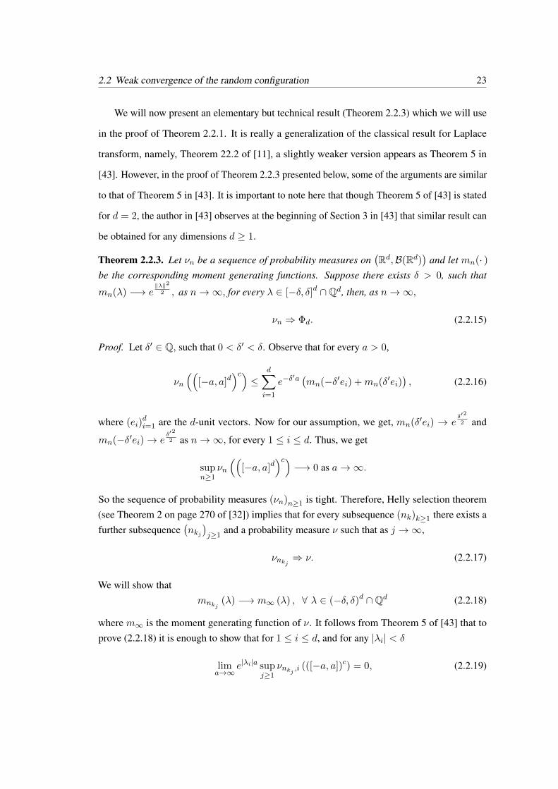
Theorem 2.2.3. Let νn be a sequence of probability measures on(Rd,B(Rd)
)and let mn(· )
be the corresponding moment generating functions. Suppose there exists δ > 0, such that
mn(λ) −→ e‖λ‖2
2 , as n→∞, for every λ ∈ [−δ, δ]d ∩Qd, then, as n→∞,
νn ⇒ Φd. (2.2.15)
Proof. Let δ′ ∈ Q, such that 0 < δ′ < δ. Observe that for every a > 0,
νn
(([−a, a]d
)c)≤
d∑i=1
e−δ′a(mn(−δ′ei) +mn(δ′ei)
), (2.2.16)
where (ei)di=1 are the d-unit vectors. Now for our assumption, we get, mn(δ′ei) → e
δ′22 and
mn(−δ′ei)→ eδ′22 as n→∞, for every 1 ≤ i ≤ d. Thus, we get
supn≥1
νn
(([−a, a]d
)c)−→ 0 as a→∞.
So the sequence of probability measures (νn)n≥1 is tight. Therefore, Helly selection theorem(see Theorem 2 on page 270 of [32]) implies that for every subsequence (nk)k≥1 there exists afurther subsequence
(nkj)j≥1
and a probability measure ν such that as j →∞,
νnkj ⇒ ν. (2.2.17)
We will show thatmnkj
(λ) −→ m∞ (λ) , ∀ λ ∈ (−δ, δ)d ∩Qd (2.2.18)
where m∞ is the moment generating function of ν. It follows from Theorem 5 of [43] that toprove (2.2.18) it is enough to show that for 1 ≤ i ≤ d, and for any |λi| < δ
lima→∞
e|λi|a supj≥1
νnkj ,i (([−a, a])c) = 0, (2.2.19)

24 Chapter 2: Central limit theorems for the urn models associated with random walks
where νnkj ,i denotes the i-th dimensional marginal for νnkj .For any |λi| < δ, we can choose δ′ ∈ Q, such that 0 < |λi| < δ′ < δ. Observe that a
calculation similar to (2.2.16) implies that for any a > 0, and for the chosen δ′
νnkj ,i (([−a, a])c) ≤ e−δ′a((mnkj
(−δ′ei) +mnkj(δ′ei)
)). (2.2.20)
Now using the assumption mn(λ) −→ e‖λ‖2
2 , as n → ∞, for every λ ∈ [−δ, δ]d ∩ Qd, weobtain,
e|λi|a supj≥1
νnkj ,i (([−a, a])c) ≤ Ke(|λi|−δ′)a, (2.2.21)
for an appropriate constant K > 0. This proves (2.2.19) and hence, (2.2.18) holds. But from ourassumption
mnkj(λ)→ e
‖λ‖22 , ∀ λ ∈ [−δ, δ]d ∩Qd.
So, we conclude that
m∞ (λ) = e‖λ‖2
2 , ∀ λ ∈ (−δ, δ)d ∩Qd.
Since both sides of the above identity are continuous functions on their respective domains,
we get that m∞ (λ) = e‖λ‖2
2 for every λ ∈ (−δ, δ)d. We know from (21.22) and Theorem30.1 of [11] for d = 1, the standard Gaussian is characterized by the values of its momentgenerating function in an open neighborhood of 0. For d ≥ 2, we can conclude that the standardGaussian distribution is characterized by the values of its moment generating function in an openneighborhood of 0, by using Theorem 30.1 of [11] and the Cramer-Wold device. So we concludethat every sub-sequential limit is standard Gaussian. This proves (2.2.15).
Proof of Theorem 2.2.1. Λn is the random probability measure on Zd ⊂ Rd, corresponding tothe random probability vector Un
n+1 . That is, for any Borel subset A of Rd,
Λn (A) =1
n+ 1
∑v∈A
Un,v.
For λ ∈ Rd, the corresponding moment generating function is given by
1
n+ 1
∑v∈Zd
e〈λ,v〉Un,v =1
n+ 1Unx (λ) =
1
n+ 1Mn (λ) Πn (e(λ)) . (2.2.22)
The moment generating function corresponding to the scaled and centered random measure Λcsnis ∑
v∈Zde〈λ, v−µ logn√
lognΣ−1/2〉 Un,v
n+ 1

2.2 Weak convergence of the random configuration 25
=1
n+ 1e−〈λ,µ
√lognΣ−1/2〉Unx
(λΣ−1/2
√log n
)(2.2.23)
=1
n+ 1e−〈λ,µ
√lognΣ−1/2〉Mn
(λΣ−1/2
√log n
)Πn
(e
(λΣ−1/2
√log n
)). (2.2.24)
To show (2.2.1), it is enough to show that for every subsequence (nk)k≥1, there exists afurther subsequence
(nkj)j≥1
such that, as j →∞,
e−〈λ,µ
√lognkj 〉
nkj + 1Mnkj
(λ√
log nkj
)Πnkj
(e
(λ√
log nkj
))−→ e
λΣλT
2 (2.2.25)
for all λ ∈ [−δ, δ]d, a.s. , where δ is as in Theorem 2.2.2. From Theorem 2.1.1, we know that
Zn − µ log n√log n
⇒ Nd (0, Σ) as n→∞.
Therefore, using (2.1.6), we obtain as n→∞,
e−〈λ,µ√
logn〉E[e〈λ, Zn√
logn〉]
=1
n+ 1e−〈λ,µ
√logn〉Πn
(e
(λ√
log n
))−→ e
λΣλT
2 .
Now using Theorem 2.2.3, it is enough to show (2.2.25) only for λ ∈ Qd ∩ [−δ, δ]d. This isequivalent to proving that for every λ ∈ Qd ∩ [−δ, δ]d, as j →∞,
Mnkj
(λ√
log nkj
)−→ 1 a.s.
From Lemma 2.2.1 we know that for all λ ∈ [−δ, δ]d
Mn
(λ√
log n
)p−→ 1 as n→∞.
Therefore, using the standard diagonalization argument we can say that given a subsequence(nk)k≥1, there exists a further subsequence
(nkj)j≥1
, such that for every λ ∈ Qd ∩ [−δ, δ]d,
Mnkj
(λ√
log nkj
)−→ 1 a.s.
This completes the proof.
Remark 2.2.1. It is worth noting here that the proofs of Theorems 2.1.1 and 2.2.1 go throughif we assume U0 to be non random probability vector such that there exists r > 0, with

26 Chapter 2: Central limit theorems for the urn models associated with random walks
∑v∈Zd e
〈λ,v〉U0,v < ∞, whenever ‖λ‖ < r. Further, if U0 is random and there exists r > 0,such that for any ‖λ‖ < r, ∑
v∈Zde〈λ,v〉U0,v <∞, a.s.
then (2.1.1) and (2.2.1) holds a.s.with respect to U0.
2.3 Rate of convergence of the central limit theorem: the Berry-Essen bound
In this section, we obtain the rate of convergence for the central limit theorem as discussed in
Theorem 2.1.1. We show that the rate of convergence is of the order O(
1√logn
), by deducing
the classical Berry-Essen type bound for any dimension d ≥ 1. The results discussed in this
section are available in [8].
2.3.1 Berry-Essen Bound for d = 1
We first consider the case when the associated random walk is a one dimensional walk and the
set of colors are indexed by the set of integers Z.
Theorem 2.3.1. Suppose U0 = δ0, then
supx∈R
∣∣∣∣P(Zn − µhn√nρ2
≤ x)− Φ (x)
∣∣∣∣ ≤ 2.75× ρ3√nρ
3/22
= O(
1√log n
), (2.3.1)
where hn :=n∑j=1
1
j + 1, Φ is the standard normal distribution function and
ρ2 :=1
n
σ2hn − µ2n∑j=1
1
(j + 1)2
(2.3.2)
and
ρ3 :=1
n
n∑j=1
1
j + 1E
[∣∣∣∣Y1 −µ
j + 1
∣∣∣∣3]
+ |µ|3n∑j=1
j
(j + 1)4
. (2.3.3)
Proof. We first note that when U0 = δ0, then (2.1.4) can be written as
Znd=
n∑j=1
IjYj (2.3.4)

2.3 Rate of convergence of the central limit theorem: the Berry-Essen bound 27
where (Yj)j≥1 are i.i.d. increments of the random walk (Sn)n≥0, (Ij)j≥1 are independent
Bernoulli variables such that Ij ∼ Bernoulli(
1j+1
)and are independent of (Yj)j≥1. Now
observe that
nρ2 =
n∑j=1
E[(IjYj − E [IjYj ])
2]
and nρ3 =
n∑j=1
E[|IjYj − E [IjYj ]|3
].
Thus from the Berry-Essen Theorem for the independent but non-identical increments (seeTheorem 12.4 of [10]), we get
supx∈R
∣∣∣∣∣P(∑n
j=1 IjYj − µhn√nρ2
≤ x
)− Φ (x)
∣∣∣∣∣ ≤ 2.75× ρ3√nρ
3/22
. (2.3.5)
The identities (2.3.4) and (2.3.5) imply the bound in (2.3.1).Finally to prove the last part of the equation (2.3.1), we note that from definition nρ2 ∼
C1 log n, and nρ3 ∼ C2 log n, where 0 < C1, C2 <∞, are some constants. Thus,
ρ3√nρ
3/22
= O(
1√log n
).
This completes the proof of the theorem.
The next result follows easily from the above theorem by observing the facts hn ∼ log n,
and nρ2 ∼ C1 log n, where C1 > 0 is a constant.
Theorem 2.3.2. Suppose U0,k = 0, for all but finitely many k ∈ Z, then there exists a constantC > 0, such that
supx∈R
∣∣∣∣P(Zn − µ log n
σ√
log n≤ x
)− Φ (x)
∣∣∣∣ ≤ C × ρ3√nρ
3/22
= O(
1√log n
), (2.3.6)
Φ is the standard normal distribution function and ρ2 and ρ3 are as defined in (2.3.2) and (2.3.3)respectively.
It is worth noting that unlike in Theorem 2.3.1 the constant C, which appears in (2.3.6)
above, is not a universal constant, it may depend on the increment distribution, as well as on U0.
Proof. Observe that
supx∈R
∣∣∣∣P(Zn − µ log n
σ√
log n≤ x
)− Φ (x)
∣∣∣∣ ≤ supx∈R
Jn(x) + supx∈R
Kn(x),

28 Chapter 2: Central limit theorems for the urn models associated with random walks
whereJn(x) =
∣∣∣∣P(Zn − µhn√nρ2
≤ xn)− Φ(xn)
∣∣∣∣ ,and xn = µ (logn−hn)√
nρ2+ xσ
√logn√nρ2
and
Kn(x) =
∣∣∣∣Φ(µ(log n− hn)√nρ2
+ xσ√
log n√nρ2
)− Φ (x)
∣∣∣∣ .From Theorem 2.3.1, we observe that
supx∈R
Jn(x) ≤ 2.75× ρ3√nρ
3/22
= O(
1√log n
). (2.3.7)
For a suitable choice of C1 > 0, we have
Kn(x) =
∣∣∣∣∣∣∣∣1√2π
µ(logn−hn)√
nρ2+xσ
√logn√nρ2∫
x
e−t22 dt
∣∣∣∣∣∣∣∣≤ C1e
−x2
2
∣∣∣∣µ(log n− hn)√nρ2
+ xσ√
log n√nρ2
− x∣∣∣∣
≤ C1
∣∣∣∣µ(log n− hn)√nρ2
∣∣∣∣+ C1e−x
2
2 |x|∣∣∣∣σ√log n√nρ2
− 1
∣∣∣∣Observe that hn = log n + γ + εn, where εn −→ 0, as n → ∞, and γ is the Euler constant.Also
√nρ2 ∼
√log n. Therefore, there exists a constant C2 > 0, such that for all n ∈ N,
C1
∣∣∣∣µ(log n− hn)√nρ2
∣∣∣∣ ≤ C2ρ3
√nρ
3/22
= O(
1√log n
). (2.3.8)
Note that the function e−x2
2 |x| attains its maximum at x = 1. Therefore,
C1e−x
2
2 |x|∣∣∣∣σ√log n√nρ2
− 1
∣∣∣∣ ≤ C1e− 1
2
∣∣∣∣σ√log n√nρ2
− 1
∣∣∣∣ .Since |
√x− 1| ≤
√|x− 1| for all x ∈ R, we obtain
C1e− 1
2
∣∣∣∣σ√log n√nρ2
− 1
∣∣∣∣ ≤ C3
√∣∣∣∣σ2 log n− nρ2
nρ2
∣∣∣∣ (2.3.9)

2.3 Rate of convergence of the central limit theorem: the Berry-Essen bound 29
for an appropriate constant C3 > 0. Observe that for some constant C4 > 0,
nρ2 − σ2 log n√nρ2
=
σ2
n∑j=1
1
j + 1− log n
− µ2n∑j=1
1
(j + 1)2
√nρ2
≤ C4ρ3
√nρ
3/22
= O(
1√log n
). (2.3.10)
Therefore, combining (2.3.8), (2.3.9) and (2.3.10) we can choose an appropriate constant C > 0,such that (2.3.6) holds.
2.3.2 Berry-Essen bound for d ≥ 2
Now, we consider the case when the associated random walk is two or higher dimensional and
the colors are indexed by Zd. Before we present our main result, we introduce a few notations.
For a matrix A = ((aij))1≤i,j≤d we denote by A (i, j), the (d− 1)× (d− 1) sub-matrix of
A, obtained by deleting the i-th row and j-th column. Let
ρ(d)2 :=
1
n
n∑j=1
1
(j + 1)
det(Σ − 1
j+1M)
det(Σ(1, 1)− 1
j+1M(1, 1)) , (2.3.11)
where M :=((µ(i)µ(j)
))1≤i,j≤d and
ρ(d)3 :=
1
nd
d∑i=1
γ3n (i)
n∑j=1
βj (i)
, (2.3.12)
where
γ2n(i) := max
1≤j≤n
det(Σ(i, i)− 1
(j+1)M(i, i))
det(Σ(1, 1)− 1
j+1M(1, 1))
and
βj(i) =1
j + 1E
∣∣∣∣∣Y (i)1 − µ(i)
j + 1
∣∣∣∣∣3+
j
(j + 1)4
∣∣∣µ(i)∣∣∣3 .
For any two vectors x and y ∈ Rd, we will write x ≤ y, if the inequality holds coordinate wise.
Theorem 2.3.3. Suppose U0 = δ0, then there exists a universal constant C (d) > 0, which may

30 Chapter 2: Central limit theorems for the urn models associated with random walks
depend on the dimension d, such that,
supx∈Rd
∣∣∣P((Zn − µhn)Σ−1/2n ≤ x
)− Φd (x)
∣∣∣ ≤ C (d)ρ
(d)3
√n(ρ
(d)2
)3/2= O
(1√
log n
),
(2.3.13)where Σn :=
∑nj=1
1j+1
(Σ − 1
j+1M)
and Φd is the distribution function of a standard d-dimensional normal random vector.
Proof. As in the one dimensional case, we start by observing that when U0 = δ0, then (2.1.4)can be written as
Znd=
n∑j=1
IjYj (2.3.14)
where (Yj)j≥1 are i.i.d. increments of the random walk (Sn)n≥0, (Ij)j≥1 are independent
Bernoulli variables such that Ij ∼ Bernoulli(
1j+1
)and are independent of (Yj)j≥1.
Now the proof of the inequality in (2.3.13) follows from equation (D) of [9] which deals withd-dimensional version of the classical Berry-Essen inequality for independent but non-identicalsummands, which in our case are the random variables (IjYj)j≥1. It is sufficient to observe that
βj(i) = E[∣∣∣IjY (i)
1 − E[IjY
(i)j
]∣∣∣3] ,and
Σn =n∑j=1
E[(IjYj − E [IjYj ])
T (IjYj − E [IjYj ])].
Finally, to prove the last part of the equation (2.3.13) as in the one dimensional case, we notethat from definition nρ(d)
2 ∼ C ′1 log n and nρ(d)3 ∼ C ′2 log n, where 0 < C ′1, C
′2 <∞, are some
constants. Thus,ρ
(d)3
√n(ρ
(d)2
)3/2= O
(1√
log n
).
This completes the proof of the theorem.
Remark 2.3.1. If we define Σ (1, 1) = 1, and M (1, 1) = 0, when d = 1, then Theorem 2.3.1follows from the above theorem except in Theorem 2.3.1 the constant is more explicit.
Just as in the one dimensional case, the following result follows easily from the above
theorem by observing hn ∼ log n.
Theorem 2.3.4. Suppose U0 = (U0,v)v∈Zd , is such that U0,v = 0 for all but finitely manyv ∈ Zd, then there exists a constant C > 0, which may depend on the increment distribution,

2.4 Urns with Colors Indexed by other lattices on Rd 31
such that
supx∈Rd
∣∣∣∣P((Zn − µ log n√log n
)Σ−1/2 ≤ x
)− Φd (x)
∣∣∣∣ ≤ C × ρ(d)3
√n(ρ
(d)2
)3/2= O
(1√
log n
),
(2.3.15)where Φd is the distribution function of a standard d-dimensional normal random vector.
Proof. Observe that
supx∈Rd
∣∣∣∣P((Zn − µ log n√log n
)Σ−1/2 ≤ x
)− Φd (x)
∣∣∣∣ ≤ supx∈Rd
Jn(x) + supx∈Rd
Kn(x),
where
Jn(x) =∣∣∣P((Zn − µhn)Σ−1/2
n ≤ xn)− Φd (xn)
∣∣∣ , (2.3.16)
where xn = µ (log n− hn)Σ−1/2n + x
√log nΣ1/2Σ
−1/2n and
Kn(x) = |Φd (xn)− Φd (x)| . (2.3.17)
It follows from Theorem 2.3.3, that
supx∈Rd
Jn(x) ≤ C (d)ρ
(d)3
√n(ρ
(d)2
)3/2= O
(1√
log n
).
Further, writing xn :=(x
(1)n , x
(2)n , . . . , x
(d)n
), we get
Kn(x) ≤d∑i=1
1√2π
∣∣∣∣∣∣∣x(i)n∫
x(i)
e−t22 dt
∣∣∣∣∣∣∣ .Note that Σn = hnΣ −
(∑nj=1
1(j+1)2
)M , so h−1
n Σn −→ Σ. The rest of the argument isexactly similar to that of the one dimensional case. This completes the proof.
2.4 Urns with Colors Indexed by other lattices on Rd
So far in this chapter, we have discussed urn models with colors indexed by Zd. We can further
generalize the urn models with colors indexed by certain countable lattices in Rd. Such a
model will be associated with the corresponding random walk on the lattice. To state the results

32 Chapter 2: Central limit theorems for the urn models associated with random walks
rigorously we consider the following notations.
Let (Yi)i≥1 be a sequence of random d-dimensional i.i.d. vectors with non empty support set
B ⊂ Rd, and probability mass function p. We assume that B is finite. Consider the countable
subset
Sd :={∑k
i=1 nibi : n1, n2, . . . , nk ∈ N, b1, b2, . . . , bk ∈ B}
of Rd, which will index the set of colors.
As earlier, we consider Sn := Y0 + Y1 + · · · + Yn, n ≥ 0, the random walk starting at Y0
and taking values now in Sd. The transition matrix for this walk is given by
R := ((p (u− v)))u,v∈Sd .
In this section, we consider an urn model (Un)n≥0 with colors indexed by Sd and replacement
matrix R. We will call this process (Un)n≥0, an infinite color urn model associated with the
random walk (Sn)n≥0 on Sd. Naturally, when Sd = Zd, this is exactly the process which is
discussed earlier.
We will use same notations as earlier for the mean, non-centered second moment matrix and
the moment generating function for the increment Y1 (see (2.0.1) for the definitions).
We will still denote by Zn, the (n+ 1)-th selected color and the expected configuration of
the urn at time n will be given by the distribution of Zn, but now on Sd.
We first note that Theorem 2.1.2 is still valid with exactly the same proof. This enable us to
generalize Theorem 2.1.1 and Theorem 2.2.1 as follows.
Theorem 2.4.1. Let Λn be the probability measure on Rd, corresponding to the probabilityvector 1
n+1 (E[Un,v])v∈Sd and let
Λcsn (A) := Λn
(√log nAΣ1/2 + µ log n
),
where A is a Borel subset of Rd. Then, as n→∞,
Λcsn ⇒ Φd. (2.4.1)
Theorem 2.4.2. Let Λn ∈M1 be the random probability measure corresponding to the random

2.4 Urns with Colors Indexed by other lattices on Rd 33
probability vector Unn+1 . Let
Λcsn (A) = Λn
(√log nAΣ1/2 + µ log n
).
where A is a Borel subset of Rd. Then, as n→∞,
Λcsnp−→ Φd inM1. (2.4.2)
The proofs of these theorems are similar to their counter part for the walks on Zd, and hence
are omitted.
We now consider a specific example, namely, the triangular lattice in two dimensions (see
Figure 2.1). For this the support set for the i.i.d. increment vectors is given by
B ={
(1, 0), (−1, 0), ω,−ω, ω2,−ω2},
where ω, ω2 are the complex cube roots of unity. The law of Y1 is uniform on B. This gives the
random walk on the triangular lattice in two dimensions.
Figure 2.1: Triangular Lattice
Following is an immediate corollary of Theorem 2.4.1.
Corollary 2.4.1. Consider the urn model associated with the random walk on two dimensionaltriangular lattice, then, as n→∞
Zn√log n
⇒ N2
(0,
1
2I2). (2.4.3)
Proof. Since 1 + ω + ω2 = 0, therefore it is immediate that µ = 0. Also we know thatω = 1
2 + i√
32 , where i is the imaginary square root of −1. Writing ω = Re (ω) + iIm (ω),

34 Chapter 2: Central limit theorems for the urn models associated with random walks
observe that E[(Y
(1)1
)2]
= 26
(1 + (Re (ω))2 +
(Re(ω2))2).
Since Re (ω) = Re(ω2), therefore, E
[(Y
(1)1
)2]
= 26
(1 + 2 (Re (ω))2
)= 1
2 . Similarly,
Im (ω) = −Im(ω2), and hence E
[(Y 2
1
)2]= 2
6
((Im (ω))2 +
(Im(ω2))2)
= 12 . Finally,
E[X
(1)1 X
(2)1
]= −2
6Im(1 + ω + ω2
)= 0. So Σ = 1
2I2. The rest is just an application of(2.4.1).

Chapter 3
Local limit theorems for the urnmodels associated with random walks 1
In this chapter, we obtain finer asymptotic properties for the distribution of the randomly
selected color and derive the local limit theorems. The local limit theorems derived here use
the representation (2.1.4). The proofs of the local limit theorems follow techniques similar to
that used in the classical case with i.i.d. increments. However, in our case the increments are
independent, but not identically distributed.
3.1 Local limit theorems for the expected configuration
Throughout this section, we consider an urn model associated with the bounded increment random
walk on Zd, d ≥ 1. In Theorem 2.1.1, it is shown that the sequence of random variables/vectors
(Zn)n≥0 satisfy the central limit theorem. In this section, we show that (Zn)n≥0 also satisfies
the local limit theorems. We first prove the local limit theorems for one dimension, and then
prove the same for dimensions higher than or equal to 2. As introduced in Chapter 2, let
Sn = Y0 +∑n
j=1 Yj , denote a random walk on Zd, with bounded increments (Yj)j≥1. For the
urn model (Un)n≥0, associated with the random walk (Sn)n≥0, the replacement matrix R is
given by (2.0.3). This section is based on [7].1This chapter is partially based on the paper entitled “Polya Urn Schemes with Infinitely Many Colors”, [7].
35

36 Chapter 3: Local limit theorems for the urn models associated with random walks
3.1.1 Local limit theorems for one dimension
In this subsection, we present the local limit theorems for urns with colors indexed by Z. As in
Chapter 2, µ, σ and e (·), will denote the mean, non-centered second moment and the moment
generating function of Y1 respectively. Note that, for Y1 a lattice random variable, we can write
P (Y1 ∈ a+ hZ) = 1, (3.1.1)
where a ∈ R and h > 0, is maximum value such that (3.1.1) holds. h is called the span for Y1
(see Section 3.5 of [28] for details on lattice random variables). We define
L(1)n :=
{x : x =
n
σ√
log na− µ
σ
√log n+
h
σ√
log nz, z ∈ Z
}. (3.1.2)
Theorem 3.1.1. Consider the urn model associated with a bounded increment random walk onZ. Assume that P (Y1 = 0) > 0. Then, as n→∞
supx∈L(1)n
∣∣∣∣σ√log n
hP(Zn − µ log n
σ√
log n= x
)− φ(x)
∣∣∣∣ −→ 0. (3.1.3)
Proof. From Theorem 2.1.2, we know thatZnd= Z0+
∑nj=1 IjYj . Yj is a lattice random variable,
therefore, IjYj is also a lattice random variable. Now by our assumption, P (Y1 = 0) > 0, wehave 0 ∈ B, where B is the support of Y1. Therefore, IjYj and Yj are supported on the samelattice.
Observe that Zn is a lattice random variable. Therefore, applying Fourier inversion formula,for all x ∈ L(1)
n , we obtain
P(Zn − µ log n
σ√
log n= x
)=
h
2πσ√
log n
πσh
√logn∫
−πσh
√logn
e−itxψn(t) dt (3.1.4)
where ψn (t) = E[eitZn−µ logn
σ√logn
]. Also, by Fourier inversion formula,
φ(x) =1
2π
∞∫−∞
e−itxe−t22 dt, for all x ∈ R. (3.1.5)

3.1 Local limit theorems for the expected configuration 37
Given ε > 0, there exists N, large enough, such that, for all n ≥ N,
∞∫σπh
√logn
φ(t) dt < ε.
Therefore, for all n ≥ N ,∣∣∣σ√log n
hP(Zn − µ log n
σ√
log n= x
)− φ(x)
∣∣∣≤ 1
2π
σπh
√logn∫
−σπh
√logn
∣∣∣ψn(t)− e−t22
∣∣∣dt+1
π
∞∫σπh
√logn
φ(t) dt
<1
2π
σπh
√logn∫
−σπh
√logn
∣∣∣ψn(t)− e−t22
∣∣∣dt+ε
π.
This implies that it is enough to prove that as n→∞
σπh
√logn∫
−σπh
√logn
∣∣∣ψn(t)− e−t22
∣∣∣dt −→ 0. (3.1.6)
Given M > 0, we can write for all n
σπh
√logn∫
−πσh
√logn
∣∣∣ψn(t)− e−t22
∣∣∣dt ≤ M∫−M
∣∣∣ψn(t)− e−t22
∣∣∣ dt+ 2
σπh
√logn∫
M
∣∣∣ψn(t)∣∣∣ dt
+2
σπh
√logn∫
M
e−t22 dt. (3.1.7)
We know from Theorem 2.1.1, that as n → ∞, Zn−µ lognσ√
logn⇒ N(0, 1). Hence, for all t ∈ R,
ψn(t) −→ e−t22 . Therefore, for any fixed M > 0, by bounded convergence theorem, we get as
n→∞,
M∫−M
∣∣∣ψn(t)− e−t22
∣∣∣dt −→ 0.

38 Chapter 3: Local limit theorems for the urn models associated with random walks
Let
I(n,M) =
σπh
√logn∫
M
∣∣∣ψn(t)∣∣∣dt. (3.1.8)
We will show that for any ε > 0, we can choose M > 0, such that for all n large enough
I(n,M) < ε. (3.1.9)
Since Znd= Z0 +
∑nj=1 IjYj , therefore,
ψn (t) = e−itµ lognσ E
[eit
Z0σ√logn
]E
[eit
∑nj=1 IjYj
σ√
logn
]. (3.1.10)
Let us denote by
gn (t) := E
[eit
∑nj=1 IjYj
σ√logn
]. (3.1.11)
It is easy to see from (3.1.10) that for all t ∈ R,∣∣∣ψn(t)∣∣∣ ≤ ∣∣∣gn (t)
∣∣∣. (3.1.12)
Therefore, from (3.1.8) we obtain
I(n,M) ≤
σπh
√logn∫
M
∣∣∣gn (t)∣∣∣dt.
Applying a change of variables t√logn
= w, we obtain,
I(n,M) ≤√
log n
πσh∫
M/√
logn
∣∣∣gn (w√log n) ∣∣∣ dw. (3.1.13)
Observe that,
E[eit∑nj=1 IjYj
]=
n∏j=1
(1− 1
j + 1+e (it)
j + 1
)=
1
n+ 1Πn (e (it))
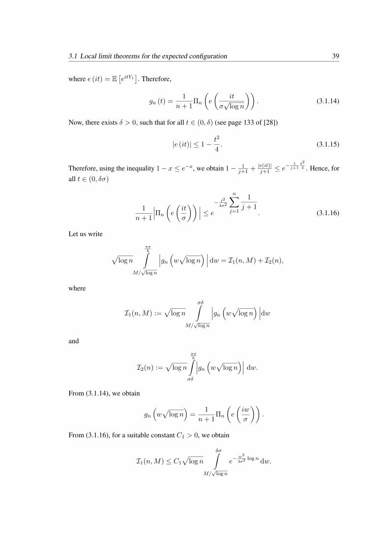
3.1 Local limit theorems for the expected configuration 39
where e (it) = E[eitY1
]. Therefore,
gn (t) =1
n+ 1Πn
(e
(it
σ√
log n
)). (3.1.14)
Now, there exists δ > 0, such that for all t ∈ (0, δ) (see page 133 of [28])
|e (it)| ≤ 1− t2
4. (3.1.15)
Therefore, using the inequality 1− x ≤ e−x, we obtain 1− 1j+1 + |e(it)|
j+1 ≤ e− 1j+1
t2
4 . Hence, forall t ∈ (0, δσ)
1
n+ 1
∣∣∣Πn
(e
(it
σ
)) ∣∣∣ ≤ e−t2
4σ2
n∑j=1
1
j + 1. (3.1.16)
Let us write
√log n
πσh∫
M/√
logn
∣∣∣gn (w√log n) ∣∣∣ dw = I1(n,M) + I2(n),
where
I1(n,M) :=√
log n
σδ∫M/√
logn
∣∣∣gn (w√log n) ∣∣∣dw
and
I2(n) :=√
log n
πσh∫
σδ
∣∣∣gn (w√log n)∣∣∣ dw.
From (3.1.14), we obtain
gn
(w√
log n)
=1
n+ 1Πn
(e
(iw
σ
)).
From (3.1.16), for a suitable constant C1 > 0, we obtain
I1(n,M) ≤ C1
√log n
δσ∫M/√
logn
e−w2
4σ2logn dw.
40 Chapter 3: Local limit theorems for the urn models associated with random walks
Applying a change of variables w√
log n = t, we obtain
I1(n,M) ≤ C1
δσ√
logn∫M
e−t2
4σ2 dt. (3.1.17)
Observe that for ε > 0, we can choose M > 0, such that
C1
∞∫M
e−t2
4σ2 dt < ε. (3.1.18)
This implies that
C1
δσ√
logn∫M
e−t2
4σ2 dt ≤ C1
∞∫M
e−t2
4σ2 dt < ε. (3.1.19)
This implies that for the chosen M ,
I1(n,M) < ε. (3.1.20)
Observe, that the span of Y1 is h. Therefore, for all t ∈[δ, 2π
h
), |e (it)| < 1. The charac-
teristic function being continuous in t, there exists 0 < η < 1, such that |e(itσ
)| ≤ η, for all
t ∈[δσ, πσh
]. Therefore,
1− 1
j + 1+|e(itσ
)|
j + 1≤ 1− 1
j + 1+
η
j + 1≤ e−
1−ηj+1 .
It follows that,
1
n+ 1
∣∣∣Πn
(e
(it
σ
)) ∣∣∣ ≤ e−n∑j=1
1− ηj + 1
≤ C2e−(1−η) logn
where C2 is some positive constant. So, as n→∞,
I2(n) ≤ C2σe−(1−η) logn (π − δ)
√log n −→ 0. (3.1.21)
Given ε > 0, choose M large enough, such that (3.1.18) holds and
∞∫M
e−t22 dt < ε.

3.1 Local limit theorems for the expected configuration 41
Therefore,
πσ√lognh∫
M
e−t2
2 dt ≤∞∫M
e−t22 dt < ε. (3.1.22)
Since (3.1.20) holds, and I2(n) −→ 0 as n→∞, therefore from (3.1.7) we obtain
limn→∞
σπh
√logn∫
−πσh
√logn
∣∣∣ψn(t)− e−t22
∣∣∣dt < 4ε. (3.1.23)
Theorem 3.1.1 covers the case when P (Y1 = 0) > 0. Suppose now, P (Y1 = 0) = 0 and let
h be the span for Y1. We can now write P (I1Y1 ∈ a+ hZ) = 1, where a ∈ R and h > 0 is the
span for I1Y1. It is easy to note that h ≤ h. The following result gives a local limit theorem for
the case when h < 2h. An example of such a walk is when P (Y1 = 1) = P (Y1 = 2) = 1/2.
Then, h = 1. The support for I1Y1 is {0, 1, 2} and h = 1. This example illustrates the case
when h < 2h holds.
Theorem 3.1.2. Assume that h < 2h, then, as n→∞
supx∈L(1)n
∣∣∣∣σ√log n
hP(Zn − µ log n
σ√
log n= x
)− φ(x)
∣∣∣∣ −→ 0, (3.1.24)
where L(1)n =
{x : x = n
σ√
logna− µ
σ
√log n+ h
σ√
lognz z ∈ Z
}.
Proof. The proof is similar to the proof of Theorem 3.1.1. So we omit certain details. Since forj ∈ N, the span of IjYj is h, for all x ∈ L(1)
n , we obtain by Fourier inversion formula,
P(Zn − µ log n
σ√
log n= x
)=
h
2πσ√
log n
πσ√lognh∫
−πσ√lognh
e−itxψn(t) dt
where ψn (t) = E[eitZn−µ logn
σ√
logn
].
Also, by Fourier inversion formula, for all x ∈ R,
φ(x) =1
2π
∞∫−∞
e−itxe−t22 dt.

42 Chapter 3: Local limit theorems for the urn models associated with random walks
The bounds for∣∣∣σ√logn
h P(Zn−µ lognσ√
logn= x
)−φ(x)
∣∣∣ are similar to those in the proof of Theorem3.1.1 except for that of I2(n), where
I2(n) =√
log n
σπh∫
σδ
∣∣∣gn (w√log n)∣∣∣ dw
and δ is chosen as in (3.1.15) and gn(·) is as in (3.1.11). We have to show
I2(n) −→ 0 as n→∞.
The span of Y1 being h, for all t ∈[δ, 2π
h
), |e (it)| < 1. We have assumed that h < 2h. The
characteristic function being continuous in t, there exists 0 < η < 1, such that, |e(itσ
)| ≤ η for
all t ∈[δσ, πσh
]⊂[δσ, 2πσ
h
). So, as n→∞,
I2(n) ≤ C2σe−(1−η) logn (π − δ)
√log n −→ 0. (3.1.25)
Remark 3.1.1. Observe that in the proof of Theorem 3.1.2, the assumption h < 2h is requiredonly to obtain the bound in (3.1.25). This assumption implies that
[δσ, πσh
]⊂[δσ, 2πσ
h
), which
guarantees the existence of 0 < η < 1, such that |e(itσ
)| ≤ η for all t ∈
[δσ, πσh
].
The next theorem is stated for the special case when the urn is associated with simple
symmetric random walk on Z, which is not covered by Theorem 3.1.1 or its generalization given
by Theorem 3.1.2.
Theorem 3.1.3. Assume that P (Y1 = 1) = P (Y1 = −1) = 12 . Then, as n→∞
supx∈L(1)n
∣∣∣∣√log nP(
Zn√log n
= x
)− φ(x)
∣∣∣∣ −→ 0 (3.1.26)
where L(1)n is given by (3.1.2) with µ = 0 = a and σ = 1 = h.
The following result is immediate from Theorem 3.1.3.
Corollary 3.1.1. Assume that P (X1 = 1) = P (X1 = −1) = 12 . Then, as n→∞
P (Zn = 0) ∼ 1√2π log n
. (3.1.27)

3.1 Local limit theorems for the expected configuration 43
Proof of Theorem 3.1.3. In this case P (Y1 = 1) = P (Y1 = −1) = 12 . Thus the span of Y1 is 2.
The random variables I1Y1 is supported on the set {0, 1,−1} and it has span 1. We have µ = 0
and σ = 1, so from (3.1.2), we get L(1)n = 1√
lognZ.
For all x ∈ L(1)n , we obtain by Fourier Inversion formula,
P(
Zn√log n
= x
)=
1
2π√
log n
π√
logn∫−π√
logn
e−itxψn(t) dt
where ψn (t) = E[eit Zn√
logn
]. Furthermore, by Fourier inversion formula, for all x ∈ R,
φ(x) =1
2π
∞∫−∞
e−itxe−t22 dt.
The proof of this theorem is also very similar to that of Theorem 3.1.1. The bounds for∣∣∣√log nP(
Zn√logn
= x)− φ(x)
∣∣∣ are similar to those in the proof of Theorem 3.1.1 except forthat of I2(n), where
I2(n) =√
log n
π∫δ
∣∣∣ψn (w√log n)∣∣∣ dw,
and δ is chosen as in (3.1.15). To show that I2(n) −→ 0 as n→∞, we observe that
E[eitZn
]=
n∏j=1
(1− 1
j + 1+
cos t
j + 1
)=
1
n+ 1Πn (cos t)
since E[eitY1
]= cos t. Therefore,
ψn(w√
log n) = E[eiwZn
]=
1
n+ 1Πn (cosw) .
We note that cosw is decreasing in[π2 , π
]and for all w ∈
[π2 , π
],−1 ≤ cosw ≤ 0. Therefore,
there exists η > 0 (small enough), such that, [π − η, π) ⊂(π2 , π
]and for all w ∈ [π − η, π), we
have −1 < cos(π − η) < 0, and∣∣∣ψn(w√
log n)∣∣∣ ≤ 1
n+ 1Πn (cos(π − η)) .

44 Chapter 3: Local limit theorems for the urn models associated with random walks
Since −1 < cos(π − η) < 0, so for all j ≥ 1,(
1 + cos(π−η)j
)< 1. Therefore,
Πn (cos(π − η)) ≤ 1. (3.1.28)
Let us writeI2(n) = J1(n) + J2(n),
where
J1(n) =√
log n
π−η∫δ
∣∣∣ψn (w√log n)∣∣∣ dw, (3.1.29)
and
J2(n) =√
log n
π∫π−η
∣∣∣ψn (w√log n)∣∣∣ dw.
It is easy to see from (3.1.28) that
J2(n) ≤ η
n+ 1
√log n −→ 0 as n→∞.
For all t ∈ [δ, π − η] , 0 ≤ |cos t| < 1, so there exists 0 < α < 1, such that, 0 ≤ |cos t| ≤ α forall t ∈ [δ, π − η]. Recall that
ψn(w√
log n) =n∏j=1
(1− 1
j + 1+
cosw
j + 1
).
Using the inequality 1− x ≤ e−x, it follows that for all t ∈ [δ, π − η]
1− 1
j + 1+|cos t|j + 1
≤ 1− 1
j + 1+
α
j + 1≤ e−
1−αj+1 ,
and hence,
1
n+ 1|Πn (cos t)| ≤ e
−
n∑j=1
1− αj + 1
≤ Ce−(1−α) logn
where C is some positive constant. Therefore, from (3.1.29) we obtain as n→∞,
J1(n) ≤ Ce−(1−α) logn (π − η − δ)√
log n −→ 0.

3.1 Local limit theorems for the expected configuration 45
3.1.2 Local limit theorems for higher dimensions
Now, we consider the case d ≥ 2. As in (2.0.1), µ, Σ and e (·), will denote the mean, non-
centered second moment matrix and the moment generating function of Y1 respectively. For Y1 a
lattice random vector taking values in Zd, let L be its minimal lattice, that is, P (Y1 ∈ x+ L) = 1
for every x ∈ Zd, such that, P (Y1 = x) > 0. We refer to the pages 226 – 227 of [10] for a
formal definition of the minimal lattice of a d-dimensional lattice random variable. If L′ is any
closed subgroup of Rd, such that P (Y1 ∈ y + L′) = 1 for some y ∈ Zd, then from the definition
of minimal lattice it follows that L ⊆ L′. We assume Y1 to be non-degenerate. This implies that
the rank of L is d. Let l = |det (L)| (see the pages 228 – 229 of [10] for more details). Now, x0
be such that, P (Y1 ∈ x0 + L) = 1 and we define
L(d)n :=
{x : x =
n√log n
x0Σ−1/2 −
√log nµΣ−1/2 +
1√log n
zΣ−1/2 : z ∈ L}.
(3.1.30)
Theorem 3.1.4. Assume that P (Y1 = 0) > 0. Then, as n→∞
supx∈L(d)n
∣∣∣∣∣det(Σ1/2)(√
log n)d
lP(Zn − µ log n√
log nΣ−1/2 = x
)− φd(x)
∣∣∣∣∣ −→ 0. (3.1.31)
Proof. From Theorem 2.1.2, we obtain Znd= Z0 +
∑nj=1 IjYj . The random vector Yj is a
lattice random vector. Therefore, IjYj is also a lattice random vector. By our assumption,P (Y1 = 0) > 0, so 0 ∈ B, therefore, Yj and IjYj are supported on the same lattice.
Observe that Zn is a lattice random vector, for every n ∈ N. For A ⊂ Rd and x ∈ R, wedefine
xA := {xy : y ∈ A},
andAΣ1/2 := {yΣ1/2 : y ∈ A}.
By Fourier inversion formula (see 21.28 on page 230 of [10]), we get for x ∈ L(d)n ,
P(Zn − µ log n√
log nΣ−1/2 = x
)=
l
(2π√
log n)ddet(Σ1/2)
∫(√
lognF∗Σ1/2)
ψn(t)e−i〈t,x〉 dt
where ψn(t) = E[ei〈t,Zn−µ logn√
lognΣ−1/2〉
], l = |det (L)| and F∗ is the fundamental domain for Y1

46 Chapter 3: Local limit theorems for the urn models associated with random walks
as defined in equation (21.22) on page 229 of [10]. Also, by Fourier inversion formula
φd(x) =1
(2π)d
∫Rd
e−i〈t,x〉e−‖t‖22 dt.
Given ε > 0, there exists N > 0 such that n ≥ N ,
∣∣∣det(Σ1/2)(√
log n)d
lP(Zn − µ log n√
log nΣ−1/2 = x
)− φd(x)
∣∣∣≤ 1
(2π)d
∫(√
lognF∗Σ1/2)
∣∣∣ψn(t)− e−‖t‖22
∣∣∣dt+1
(2π)d
∫Rd\√
lognF∗Σ1/2
e−‖t‖22 dt
≤ 1
(2π)d
∫(√
lognF∗Σ1/2)
∣∣∣ψn(t)− e−‖t‖22
∣∣∣dt+ ε.
Therefore, it is enough to prove that as n→∞∫(√
lognF∗Σ1/2)
∣∣∣ψn(t)− e−‖t‖22
∣∣∣ dt −→ 0. (3.1.32)
Given any compact set A ⊂ Rd, we have∫(√
lognF∗Σ1/2)
∣∣∣ψn(t)− e−‖t‖22
∣∣∣ dt ≤ ∫A
∣∣∣ψn(t)− e−‖t‖22
∣∣∣ dt+
∫(√
lognF∗Σ1/2)\A
∣∣∣ψn(t)∣∣∣ dt
+
∫Rd\A
e−‖t‖22 dt. (3.1.33)
By Theorem 2.1.1, we know that Zn−µ logn√logn
Σ−1/2 ⇒ Nd(0, Id) as n→∞. Therefore, for anycompact set A ⊂ Rd, by bounded convergence theorem,∫
A
∣∣∣ψn(t)− e−‖t‖22
∣∣∣dt −→ 0 as n→∞.
Let us write
I(n,A) =
∫(√
lognF∗Σ1/2)\A
∣∣∣ψn(t)∣∣∣dt. (3.1.34)
We will show that for any ε > 0, we can choose a compact subset A of Rd, such that for all n

3.1 Local limit theorems for the expected configuration 47
large enough
I(n,A) < ε.
Since Znd= Z0 +
∑nj=1 IjYj , calculations similar to (3.1.10) show that for every t ∈ Rd, and
each n ∣∣∣ψn(t)∣∣∣ ≤ ∣∣∣gn(t)
∣∣∣,where
gn (t) := E
[e〈it,
∑nj=1 IjYj√
lognΣ−1/2〉
]. (3.1.35)
Therefore, from (3.1.34) we obtain
I(n,A) ≤∫
(√
lognF∗Σ1/2)\A
∣∣∣gn(t)∣∣∣ dt. (3.1.36)
Observe that
E[ei〈t,
∑nj=1 IjYj〉
]=
n∏j=1
(1− 1
j + 1+e (it)
j + 1
)=
1
n+ 1Πn (e (it))
where e (it) = E[ei〈t,Y1〉
]. So, from (3.1.35)
gn(t) =1
n+ 1Πn
(e
(1√
log nitΣ−1/2
)).
Applying a change of variables t = 1√logn
w, to (3.1.34), we obtain
I(n,A) ≤ (√
log n)d∫
F∗Σ1/2\ 1√logn
A
∣∣∣gn (√log nw) ∣∣∣ dw. (3.1.37)
We can choose δ > 0, such that for all w ∈ B(0, δ) \ {0}, there exists b > 0, such that
|e(iw)| ≤ 1− b‖w‖2
2, (3.1.38)
(see Lemma 2.3.2(a) of [46] for a proof). Therefore, using the inequality 1− x ≤ e−x,
|gn(√
log nw)| =1
n+ 1|Πn
(e(iwΣ−1/2)
)|

48 Chapter 3: Local limit theorems for the urn models associated with random walks
≤n+1∏j=1
(1− 1
j + 1+|e(iwΣ−1/2
)|
j + 1
)
≤ e
−
n∑j=1
b
j + 1
‖w‖2
2≤ C1e
−bwΣwT
2logn (3.1.39)
for some positive constant C1. We write
(√
log n)d∫
F∗Σ1/2\ 1√logn
A
∣∣∣gn (√log nw) ∣∣∣ dw = I1(n,A) + I2(n)
where
I1(n,A) := (√
log n)d∫
(B(0,δ)Σ1/2\ 1√
lognA)∩F∗Σ1/2
|gn(√
log nw)|dw
and
I2(n) = (√
log n)d∫
F∗Σ1/2\B(0,δ)Σ1/2
|gn(√
log nw)|dw.
From (3.1.39), we obtain
I1(n) ≤ C1(√
log n)d∫
B(0,δ)Σ1/2\ A√logn
e−bwΣwT
2logn dw, (3.1.40)
for an appropriate positive constant C1. Applying a change of variables w(√
log n)
= t, weobtain
I1(n,A) ≤ C1
∫B(0,δ
√logn)Σ1/2\A
e−bwΣwT
2 dw. (3.1.41)
Given ε > 0, choose a compact subset A of Rd, such that
C1
∫Ac
e−bwΣwT
2 dw < ε. (3.1.42)
Therefore, for this choice of A,I1(n,A) < ε. (3.1.43)
Since the lattices for Y1 and I1Y1 are same, for all w ∈ F∗ \ B(0, δ), we get |e(iw)| < 1, sothere exists an 0 < η < 1, such that, |e(iwΣ−1/2)| ≤ η, for all w ∈ F∗Σ1/2 \ B(0, δ)Σ1/2
3.1 Local limit theorems for the expected configuration 49
Therefore, using the inequality 1− x ≤ e−x, we obtain
|gn(√
log nw)| ≤ e−∑nj=i
1j+1
(1−η) ≤ C2e−(1−η) logn (3.1.44)
for some positive constant C2. Therefore, using equation (21.25) on page 230 of [10], we obtain
I2(n) ≤ C ′2(√
log n)de−(1−η) logn −→ 0 as n→∞ (3.1.45)
where C ′2 is an appropriate positive constant.Given ε > 0, choose A, such that, (3.1.42) holds and∫
Ac
e−‖t‖22 dt < ε. (3.1.46)
From (3.1.33), (3.1.43), (3.1.45) and (3.1.46), we get
limn→∞
∫(√
lognF∗Σ1/2)
∣∣∣ψn(t)− e−‖t‖22
∣∣∣dt < 2ε. (3.1.47)
Observe that as in the one dimensional case, Theorem 3.1.4 covers only the case when
P (Y1 = 0) > 0. The next theorem is stated for the special case when the urn is associated with
simple symmetric random walk on Zd, d ≥ 2, which is not covered by the Theorem 3.1.4.
Theorem 3.1.5. Assume that P (Y1 = ±ei) = 12d , for 1 ≤ i ≤ d, where ei is the i-th unit vector
in direction i. Then, as n→∞,
supx∈L(d)n
∣∣∣∣∣(d)d2
(√log n
)dP
( √d√
log nZn = x
)− φd(x)
∣∣∣∣∣ −→ 0, (3.1.48)
where L(d)n is as defined in (3.1.30) with µ = 0 = x0, Σ = Id and L =
√dZd.
Similar to the one dimensional case, the next result is immediate from the above theorem.
Corollary 3.1.2. Assume that P (X1 = ±ei) = 12d , for 1 ≤ i ≤ d, where ei is the i-th unit
vector in direction i. Then, as n→∞,
P (Zn = 0) ∼ 1(√2πd log n
)d . (3.1.49)
Proof of Theorem 3.1.5. In this case, P (Y1 = ±ei) = 12d , for 1 ≤ i ≤ d, where ei is the i-th
unit vector in direction i, thus µ = 0 and Σ = 1dId.

50 Chapter 3: Local limit theorems for the urn models associated with random walks
For notational simplicity, we prove (3.1.48) for d = 2. The proof for general d can be writtensimilarly.
Now for each j ∈ N, IjYj is a lattice random vector with the minimal lattice Z2. It is easy tosee that 2πZ × 2πZ is the set of all periods for IjYj , and its fundamental domain is given by(−π, π)2. To prove (3.1.48), it is enough to show
supx∈ 1√
2L(2)n
∣∣∣∣(log n)P(
Zn√log n
= x
)− φ2, 1
2I2(x)
∣∣∣∣ −→ 0 as n→∞,
where φ2, 12I2(x) = 1
πe−‖x‖2 is the bivariate normal density with mean vector 0 and variance-
covariance matrix 12I2 and 1√
2L(2)n = 1√
lognZ2. By Fourier inversion formula (see 21.28 on page
230 of [10]), we get for x ∈ 1√2L(2)n
P(
Zn√log n
= x
)=
1
(2π)2 log n
∫(−√
lognπ,√
lognπ)2
ψn(t)e−i〈t,x〉 dt
Also, by Fourier inversion formula,
φ2, 12I2(x) =
1
(2π)2
∫R2
e−i〈t,x〉e−‖t‖24 dt.
Let us write Hn =(−√
log nπ,√
log nπ)2. Given ε > 0, there exists N > 0, such that, for
n ≥ N ,∣∣∣ log nP(
Zn√log n
= x
)− φ2, 1
2I2(x)
∣∣∣ ≤ 1
(2π)2
∫Hn
∣∣∣ψn(t)− e−‖t‖24
∣∣∣dt+1
(2π)2
∫R2\Hn
e−‖t‖24 dt
<1
(2π)2
∫Hn
∣∣∣ψn(t)− e−‖t‖24
∣∣∣dt+ ε.
Given any compact set A ⊂ R2, for all n large enough, we have∫Hn
∣∣∣ψn(t)− e−‖t‖24
∣∣∣ dt ≤ ∫A
∣∣∣ψn(t)− e−‖t‖24
∣∣∣ dt+
∫Hn\A
∣∣∣ψn(t)∣∣∣ dt+
∫Ac
e−‖t‖24 dt.
By Theorem 2.1.1, we know that Zn√logn⇒ N2(0, 1
2I2), as n→∞. Therefore, for any compactset A ⊂ R2, by bounded convergence theorem,∫
A
∣∣∣ψn(t)− e−‖t‖24
∣∣∣dt −→ 0 as n→∞.

3.1 Local limit theorems for the expected configuration 51
Let us write
I(n,A) =
∫Hn\A
∣∣∣ψn(t)∣∣∣dt.
We will show that for any ε > 0, we can choose a compact subset A of R2, such that, for alln large enough ∫
Ac
e−‖t‖24 dt < ε,
and
I(n,A) < ε.
Applying a change of variables t = 1√logn
w, we obtain
I(n,A) = logn
∫(−π,π)2\ 1√
lognA
∣∣∣ψn (√log nw) ∣∣∣dw.
We can write
I(n,A) = I1(n,A) + I2(n)
where
I1(n,A) = log n
∫(B(0,δ)\ 1√
lognA)∩(−π,π)2
|ψn(√
log nw)| dw
and
I2(n) = log n
∫(−π,π)2\B(0,δ)
|ψn(√
log nw)|dw.
where δ is as in (3.1.38). Using arguments similar to (3.1.43), we can show that for any ε > 0,
we can choose a compact subset A of R2, such that for all n large enough
I1(n,A) < ε.
Therefore, it is enough to show that I2(n) −→ 0, as n → ∞. To do so, we first ob-serve that for t =
(t(1), t(2)
)∈ R2, the characteristic function for Y1 is given by

52 Chapter 3: Local limit theorems for the urn models associated with random walks
e (it) = 12
(cos t(1) + cos t(2)
). So, if t ∈ [−π, π]2, be such that, |e (it)| = 1, then
t ∈ {(π, π), (−π, π), (π,−π), (−π,−π)}. The function cos θ is continuous and decreasingas a function of θ for θ ∈
[π2 , π
]. Choose η > 0, such that for t ∈ A1 = (−π, π)2 ∩
Bc(0, δ) ∩ Dc, we have |e (it)| < 1, where D = [π − η, π)2 ∪ [−π + η,−π) × [π − η, π) ∪[−π + η,−π)2 ∪ [π − η, π)× [−π + η,−π). Let us write
I2(n) = J1(n) + J2(n),
where
J1(n) = log n
∫A1
|ψn(√
log nw)|dw
and
J2(n) = logn
∫D
|ψn(√
log nw)|dw.
It is easy to note that,
J1(n) ≤ log n
∫A1
|ψn(√
log nw)|dw,
where A1 denotes the closure of A1. For w ∈ A1, there exists some 0 < α < 1, such that,|e (it)| ≤ α. Therefore, using bounds similar to that in (3.1.44), we can show that
J1(n) −→ 0 as n→∞.
We observe thatJ2(n) ≤ 4 log n
∫[π−η,π]2
|ψn(√
log nw)|dw.
Hence, it is enough to show that
log n
∫[π−η,π]2
|ψn(√
log nw)|dw −→ 0 as n→∞.
For w ∈ [π − η, π]2, we have 0 < |(
1 + e(iw)j
)| ≤
(1 + cos(π−η)
j
)≤ 1. Therefore,
|ψn(√
log nw)| = 1
n+ 1
n∏j=1
∣∣∣ (1 +e(iw)
j
) ∣∣∣ ≤ 1
n+ 1.

3.1 Local limit theorems for the expected configuration 53
So,
log n
∫[π−η,π]2
|ψn(√
log nw)|dw ≤ η2
n+ 1log n −→ 0 as n→∞.

54 Chapter 3: Local limit theorems for the urn models associated with random walks

Chapter 4
Large deviation principle for the urnmodels associated with random walks1
Urn models associated with bounded increment random walks were introduced in Chapter 2. Let
Sn = Y0 +∑n
j=1 Yj , denote a random walk on Zd, with bounded increments (Yj)j≥1. For the
urn model (Un)n≥0, associated with the random walk (Sn)n≥0, we consider the replacement
matrix R given by (2.0.3). As in (2.0.1), µ, Σ and e (·), will denote the mean, non-centered
second moment matrix and the moment generating function of Y1 respectively. For this model,
as shown in Theorem 2.1.1, if Zn is the randomly selected color at the (n+ 1)-th draw, then
Zn − µ log n√log n
⇒ Nd (0, Σ) as n→∞. (4.0.1)
It is easy to see that (4.0.1) implies
Znlog n
p−→ µ as n→∞. (4.0.2)
In the following section, we show that the sequence of probability measures(P(Zn
logn ∈ ·))
n≥2
satisfy a large deviation principle (LDP) with a good rate function and speed log n. A character-
ization of the rate function is also provided.
The large deviation principle discussed here uses the representation (2.1.4). Since the
increments (IjYj)j≥1 are independent, but not identically distributed, we require techniques
1This chapter is based on the paper “ Rate of convergence and large deviation for the infinite color Polya urnschemes, Statist. Probab. Lett., 92:232-240, 2014, [8].
55

56 Chapter 4: Large deviation principle for the urn models associated with random walks
different from the classical case. For this we use the Gartner-Ellis Theorem (see Remark (a) on
page 45 of [27] or page 66 of [16]).
4.1 Large deviation principles for the randomly selected color
The following standard notation is used in this section. For any subset A ⊆ Rd, we write A◦ to
denote the interior of A and A to denote the closure of A, under the usual Euclidean topology.
We present a few definitions (for more details see [27]), which are standard in the literature.
Definition 4.1.1. A sequence of probability measures (νn)n≥2 is said to satisfy a LDP with arate function I , and speed vn, if for all Borel subset A of Rd,
− infx∈A◦
I(x) ≤ limn→∞
log νn (A)
vn≤ lim
n→∞
log νn (A)
vn≤ − inf
x∈AI(x).
Definition 4.1.2. A rate function I is a lower semicontinuous function I : Rd → [0,∞]. A ratefunction is said to be good, if all the level sets {x : I(x) ≤ a} are compact subsets of Rd.
In the next theorem, we discuss the asymptotic behavior of the tail probabilities of Znlogn .
Theorem 4.1.1. The sequence of probability measures(P(Zn
logn ∈ ·))
n≥2satisfy a LDP with
rate function I (·) and speed log n, where I(·) is the Fenchel-Legendre dual of e (·)− 1, that is,for x ∈ Rd,
I(x) = supλ∈Rd{〈x, λ〉 − e(λ) + 1}. (4.1.1)
Moreover, I(·) is a good rate function which is also convex.
Proof. Let us define
αn (λ) :=1
log nlogE
[e〈λ,Zn〉
]. (4.1.2)
From (2.1.4), we know that
Znd= Z0 +
n∑j=1
IjYj .
Therefore, it follows from calculations similar to (2.1.5)
E[e〈λ,Zn〉
]=
1
n+ 1E[e〈λ,Z0〉
]Πn (e (λ))
where Πn (z) =∏nj=1
(1 + z
j
), z ∈ C. From (2.1.3), we get
αn (λ) −→ e (λ)− 1 <∞, ∀ λ ∈ Rd. (4.1.3)

4.1 Large deviation principle for the randomly selected color 57
Thus the LDP now follows from the Gartner-Ellis Theorem (see Remark (a) on page 45 of [27]or page 66 of [16]).
We next note that I(·) is a convex function because it is the Fenchel-Legendre dual ofe (λ)− 1, which is finite for all λ ∈ Rd.
Finally, we will show that I (·) is good rate function, that is, the level sets A (a) =
{x : I(x) ≤ a} are compact for all a > 0. The function I is a rate function. Hence bydefinition, it is lower semicontinuous. So, it is enough to prove that, A(a) is bounded for alla ∈ R. Observe that, for all x ∈ Rd,
I(x) ≥ sup‖λ‖=1
{〈x, λ〉 − e(λ) + 1} .
Now the function λ 7→ e (λ) is continuous and {λ : ‖λ‖ = 1} is a compact set. So ∃ λ0 ∈{λ : ‖λ‖ = 1}, such that sup‖λ‖=1 e (λ) = e (λ0). Therefore, for ‖x‖ 6= 0, choosing λ = x
‖x‖ ,we have I(x) ≥ ‖x‖ − e (λ0) + 1. So, if x ∈ A(a), then,
‖x‖ ≤ (a+ e (λ0)− 1) .
This proves that the level sets are bounded, which completes the proof.
Our next result is an easy consequence of (4.1.1) which can be used to compute explicit
formula for the rate function I .
Theorem 4.1.2. The rate function I is same as the rate function for the large deviation of theempirical means of i.i.d. random vectors with distribution corresponding to the distribution ofthe following random vector
W =
N∑i=1
Yi, (4.1.4)
where N ∼ Poisson (1) and is independent of (Yj)j≥1, which are the i.i.d. increments of theassociated random walk.
Proof. We first observe that logE[e〈λ,W 〉
]= e (λ)− 1. The rest then follows from (4.1.1) and
Cramer’s Theorem (see Theorem 2.2.30 of [27]).
For d = 1, one can get more information about the rate function I , in particular the following
result is a consequence of Theorem 4.1.2 and Lemma 2.2.5 of [27].
Proposition 4.1.1. Suppose d = 1, then I(x) is non-decreasing when x ≥ µ and non-increasing

58 Chapter 4: Large deviation principle for the urn models associated with random walks
when x ≤ µ. Moreover,
I(x) =
supλ≥0{xλ− e(λ) + 1} if x ≥ µ,
supλ≤0{xλ− e(λ) + 1} if x ≤ µ.
(4.1.5)
In particular, I(µ) = infx∈R I(x).
The following is an immediate corollary of the above result and Theorem 4.1.1.
Corollary 4.1.1. Let d = 1, then for any ε > 0,
limn→∞
1
log nlogP
(Zn
log n≥ µ+ ε
)= −I (µ+ ε) , (4.1.6)
andlimn→∞
1
log nlogP
(Zn
log n≤ µ− ε
)= −I (µ− ε) . (4.1.7)
We end the chapter with explicit computations of the rate functions for two examples of
infinite color urn models associated with random walks on one dimensional integer lattice.
Example 4.1.1. Our first example is the case when the random walk is the right shift asintroduced in Subsection 1.2.1, which moves deterministically one step to the right at a time. Inother words, Y1 = 1, with probability one. In this case µ = 1 and σ2 = 1. Also the momentgenerating function of Y1, is given by e (λ) := eλ, λ ∈ R. By Theorem 4.1.2, the rate functionfor the associated infinite color urn model is same as the rate function for a Poisson randomvariable with mean 1 (see page 96 of [28]), that is,
I(x) =
∞ if x < 0,
1 if x = 0,
x log x− x+ 1 if x > 0.
(4.1.8)
Example 4.1.2. Our next example is the case when the random walk is the simple symmetricrandom walk on the one dimensional integer lattice. For this case, we note that µ = 0, σ2 = 1
and the moment generating function Y1 is e (λ) = coshλ, λ ∈ R. Therefore, from (4.1.5), wehave
I(x) =
supλ≥0{xλ− coshλ+ 1} if x ≥ 0,
supλ≤0{xλ− coshλ+ 1} if x ≤ 0.
Fixing x ∈ R, define fx (λ) := xλ − coshλ + 1. Differentiating fx (λ) with respect to λ, we

4.1 Large deviation principle for the randomly selected color 59
obtaindfx (λ)
dλ= x− sinhλ, (4.1.9)
andd2fx (λ)
dλ2= − coshλ < 0 for all λ ∈ R. (4.1.10)
λ = sinh−1 x, solves the equation dfx(λ)dλ = 0, for every fixed x ∈ R. Therefore, the function
fx (λ) attains its maximum at λ = sinh−1 x. Hence, the rate function for the associated infinitecolor urn model turns out to be
I(x) = x sinh−1 x−√
1 + x2 + 1. (4.1.11)

60 Chapter 4: Large deviation principle for the urn models associated with random walks

Chapter 5
Representation theorem 1
In this chapter, we present a coupling of the urn model with the associated Markov chain,
which will improve the representation given in (2.1.4). This method is novel and useful in
deriving several results for the expected configuration of the urn. There are a few standard
methods for analyzing finite color urn models which are mainly based on martingale techniques
[38, 55, 14, 15, 25], stochastic approximations [44] and embedding into continuous time pure
birth processes [3, 40, 41, 5]. Typically, the analysis of a finite color urn is heavily dependent on
the Jordan decomposition [24] of matrices and the Perron-Frobenius theory [58] of matrices with
positive entries, [3, 38, 40, 41, 5, 14, 25]. The absence of such theories for infinite dimensional
matrices makes the analysis of urns with infinitely many colors quite difficult and challenging.
The improved representation derived here will help us bypass this difficulty.
5.1 Representation theorem
Theorem 5.1.1. Consider an urn model with colors indexed by a set S, replacement matrix Rand initial configuration U0. Let (Xn)n≥0 be the associated Markov chain. Then, there exists anincreasing non negative sequence of stopping times (τn)n≥0 with τ0 = 0, which are independentof the Markov chain (Xn)n≥0, such that, if Zn denotes the color of the (n+ 1)-th selected ball,then, for any n ≥ 0,
Znd= Xτn . (5.1.1)
1This chapter is based on the paper entitled “A New Approach to Polya Urn Schemes and Its Infinite ColorGeneralization”, [6].
61

62 Chapter 5: Representation theorem
Moreover, as n→∞,τn
log n−→ 1 a.s. (5.1.2)
andτn − log n√
log n⇒ N (0, 1) . (5.1.3)
Remark 5.1.1. Theorem 5.1.1 will be referred to as the representation theorem. It is worthwhileto note here that (5.1.1) gives only a marginal representation of Zn, for each n ≥ 0. Thefollowing need not be true:
(Zn)n≥0d= (Xτn)n≥0 . (5.1.4)
This is because (Xτn)n≥0 is a Markov chain, but (Zn)n≥0 is not necessarily Markov.
Observe that the probability mass function for Zn is(E[Un,v ]n+1
)v∈S
. Therefore (5.1.1) will be
useful in deriving results about the expected configuration of the urn. However, the representation
theorem may not be useful in deriving asymptotic properties of the random configuration of
the urn. It is worthwhile to note here that Theorem 5.1.1 holds for any S, be it finite or infinite.
Consequently, (5.1.1) will be used in the next section to rederive several known results for finite
colors. In the next chapter, we will apply Theorem 5.1.1 to derive new results for the infinite
color case.
Proof of Theorem 5.1.1. It is clear that the probability mass function for Zn is given by(E[Un,v ]n+1
)v∈S
. From (1.1.4), we have
Un = Un−1 + χnR.
Denote by R (u, v) the v-th entry of the u-th row of the matrix R, for all u, v ∈ S. So,
Unn+ 1
=n
n+ 1
Un−1
n+
1
n+ 1χnR
=n
n+ 1
Un−1
n+
1
n+ 1R (Zn−1, ·) . (5.1.5)
We will prove this theorem by induction on n ∈ N. Let (Xn)n≥0 be the Markov chain associatedwith the urn process. Then the initial distribution of (Xn)n≥0 is given by U0. Let us denote byPU0 the law of the Markov chain (Xn)n≥0. We know that the distribution of Z0 is given by U0.Therefore, (5.1.1) is trivially true for n = 0.
Let (Ij)j≥1 be a sequence of independent Bernoulli random variables, with E [Ij ] = 1j+1 ,
such that (Ij)j≥1 is independent of (Xn)n≥0 . Define τn =∑n
j=1 Ij , and τ0 ≡ 0. Observe that,

5.1 Representation theorem 63
the law of τn is same as in Lemma 1.2.1. It is easy to see that,
PU0 (Xτ1 = v) = PU0 ((1− I1)X0 + I1X1 = v)
=1
2PU0 (X0 = v) +
1
2PU0 (X1 = v) (5.1.6)
The distribution of Z0 is given by (U0,v)v∈S , therefore
E [R (Z0, v)] = PU0 (X1 = v) . (5.1.7)
Using equations (5.1.5), (5.1.6) and (5.1.7), we have proved (5.1.1) for n = 1. Let us assumethat the result is true for n, that is,
Znd= Xτn . (5.1.8)
We want to showZn+1
d= Xτn+1 .
We know that the distribution of Zn+1 is given by 1n+2 (E [Un+1,v])v∈S . For v ∈ S, we have
PU0
(Xτn+1 = v
)= PU0 ((1− In+1)Xτn + In+1Xτn+1 = v)
=n+ 1
n+ 2PU0 (Xτn = v) +
1
n+ 2PU0 (Xτn+1 = v) .
By assumption (5.1.8), we have
R (Zn, v) = P (Xτn+1 = v|Xτn) .
Therefore,E [R (Zn, v)] = PU0 (Xτn+1 = v) .
This proves (5.1.1).Now we will show (5.1.2) and (5.1.3). As observed in (1.2.6),
E [τn] ∼ log n as n→∞. (5.1.9)
From (1.2.7), we obtain
Var (τn) =∑n
j=11j+1 −
1(j+1)2
∼ log n as n→∞. (5.1.10)
Observe that,
∑n≥1
Var(In)
(log n)2 ≤∑n≥1
1
(n+ 1) (log n)2 <∞.

64 Chapter 5: Representation theorem
Therefore, by the Strong Law of Large Numbers for independent random variables (see Theorem2 on page 364 of [59]), we obtain as n→∞,
τn − E [τn]
log n−→ 0 a.s. (5.1.11)
From (1.2.6), we have E[τn]logn −→ 1 as n → ∞. This together with (5.1.11) implies that as
n→∞,
τnlog n
−→ 1 a.s.
This proves (5.1.2). The conclusion in (5.1.3) follows from Lemma 1.2.1.
The following proposition is immediate from the proof of Theorem 5.1.1.
Proposition 5.1.1. Under the assumptions made in Theorem 5.1.1, it is possible to choose(τn)n≥1, such that, for all n ≥ 1,
τn =
n∑j=1
Ij . (5.1.12)
where (Ij)j≥1 is a sequence of independent Bernoulli random variables, with E [Ij ] = 1j+1 , and
(Ij)j≥1 is independent of (Xn)n≥0.
5.2 Color count statistics
For every v ∈ S, and n ≥ 0, let
Nn,v :=
n∑m=0
1{Zm=v}
denote the color count statistics for v. Note that for every n ≥ 0,
∑v∈S
Nn,v = n+ 1.
Here, we present some results for the color count statistics, for both finite and infinite color
urn models.
Lemma 5.2.1. Consider an urn model with colors indexed by a set S, replacement matrix Rand initial configuration U0. If Zn denotes the color of the (n + 1)-th selected ball, then for

5.2 Color count statistics 65
every v ∈ S,
limn→∞
(Un,vn+ 1
− 1
n+ 1
∑u∈S
Nn,uR(u, v)
)= 0, a.s. (5.2.1)
where R(u, v) denotes the v-th element of the u-th row of R.
Proof. For n ≥ 0, the following is obvious from (1.1.4)
Un+1 = Un + χn+1R = U0 +
n+1∑k=1
χkR.
Writing χn = (χn,u)u∈S , we observe that χn,u = 1{Zn−1=u} for every u ∈ S. Therefore, itfollows that
Un,v = U0,v +∑u∈S
n∑m=0
1{Zm=u}R(u, v) = U0,v +∑u∈S
Nn,uR(u, v). (5.2.2)
This implies that, as n→∞,(Un,vn+ 1
− 1
n+ 1
∑u∈S
Nn,uR(u, v)
)=
U0,v
n+ 1−→ 0 a.s. (5.2.3)
Remark 5.2.1. It is worthwhile to note that the identity (5.2.2) imply that (5.2.1) holds for everyrealization.
Corollary 5.2.1. Consider an urn model with colors indexed by a set S, replacement matrix Rand initial configuration U0. Let π = (πu)u∈S be a solution to πR = π, such that πu ≥ 0, foreach u ∈ S. If for all v ∈ S,
Nn,v
n+ 1−→ πv a.s. as n→∞, (5.2.4)
then, for every v ∈ S,Un,vn+ 1
−→ πv a.s. as n→∞. (5.2.5)
Remark 5.2.2. For infinitely many colors, it is well known from the standard theory of Markovchains (see page 130 of [11]) that there exists a unique solution π = (πu)u∈S , with πu > 0, foreach u ∈ S and
∑u∈S πu = 1 to
πR = π,
if and only if, R is irreducible and positive recurrent. However, if R is irreducible and nullrecurrent, then πu = 0, for all u ∈ S.

66 Chapter 5: Representation theorem
Proof of Corollary 5.2.1. Assume (5.2.4) holds, then to prove (5.2.5), we observe that from(5.2.1), it is enough to prove that, for every v ∈ S,
limn→∞
1
n+ 1
∑u∈S
Nn,uR(u, v) = πv a.s. (5.2.6)
From (5.2.4), we know that for every u ∈ S, as n→∞,
Nn,u
n+ 1−→ πu a.s.
Therefore, by dominated convergence theorem, it follows that, as n→∞,
1
n+ 1
∑u∈S
Nn,uR(u, v) −→ πv a.s. (5.2.7)
for every v ∈ S.
Corollary 5.2.2. Consider an infinite color urn model with colors indexed by a set S, replace-ment matrix R and initial configuration U0. Let R be irreducible. Then, the following areequivalent:
(i) For every v ∈ S, limn→∞
Un,vn+ 1
= 0 a.s.;
(ii) For every v ∈ S, limn→∞
Nn,v
n+ 1= 0 a.s.
Proof. First we prove that (i) implies (ii). Fix v ∈ S. Since R is irreducible, given v ∈ S, thereexists u ∈ S, such that R(v, u) > 0. Since we have assumed (i) holds, we have
limn→∞
Un,un+ 1
= 0.
Therefore, (5.2.1) implies that for this chosen u ∈ S,
limn→∞
1
n+ 1
∑w∈S
Nn,wR(w, u) = 0 a.s. (5.2.8)
Since, for every w ∈ S, Nn,wR(w, u) ≥ 0, therefore, (5.2.8) implies that,
limn→∞
1
n+ 1Nn,wR(w, u) = 0. (5.2.9)
Since R(v, u) > 0, (5.2.9) implies that,
limn→∞
Nn,v
n+ 1= 0 a.s. (5.2.10)

5.3 Applications of the representation theorem for finite color urn models 67
This proves that (i) implies (ii).The proof that (ii) implies (i) is similar to the proof of Corollary 5.2.1.
Remark 5.2.3. It is worthwhile to note here that if R is reducible, then it may happen that
limn→∞
Un,vn+ 1
= 0 a.s. for some but not all v. (5.2.11)
Consider the following example where the S = N and R = ((R(i, j)))i,j∈N, such that
R(i, j) =
1 if i = 1, j ∈ N,
0 otherwise.
In this case, it follows trivially that
limn→∞
Un,1n+ 1
= 1, a.s.
and for all j ≥ 2,
limn→∞
Un,jn+ 1
= 0, a.s.
5.3 Applications of the representation theorem for finite color urnmodels
We will now present some applications of the representation theorem for finite color urn models.
These results are already available in literature, we will give alternative proofs as applications
of the representation theorem. More applications leading to new results for infinite color urn
models are available in Chapter 6.
5.3.1 Irreducible and aperiodic replacement matrices
Theorem 5.3.1. Consider an urn model with colors indexed by {1, 2, . . . ,K}. Let R be ir-reducible, and aperiodic, with a unique stationary distribution π = (πj)1≤j≤K . Then, asn→∞,
P (Zn = j) −→ πj , for every j ∈ {1, 2, . . . ,K} . (5.3.1)
The proof (5.3.1) is available in [3, 38, 40, 5] using techniques different from the representa-
tion (5.1.1). Here, we present the proof as an application of (5.1.1).

68 Chapter 5: Representation theorem
Proof. Since (Xn)n≥0 is irreducible and aperiodic, therefore using the standard limit theoremsfor Markov chains, see [11], we have as n→∞,
P (Xn = j) −→ πj , for every j ∈ {1, 2, . . . ,K} . (5.3.2)
From (5.1.1), we know that Znd= Xτn , where (τn)n≥1 is independent of (Xn)n≥0 . From (5.1.2),
we know that τn −→∞, as n→∞. This together with (5.3.2) implies that, as n→∞,
P (Zn = j) = P (Xτn = j) −→ πj , (5.3.3)
j ∈ {1, 2, . . . ,K}. This completes the proof.
Corollary 5.3.1. Consider an urn model with colors indexed by {1, 2, . . . ,K}. Let R beirreducible, and aperiodic, with a unique stationary distribution π = (πj)1≤j≤K . Then, asn→∞,
E [Nn,j ]
n+ 1−→ πj , for all 1 ≤ j ≤ K. (5.3.4)
Proof.
E [Nn,j ] =
n∑m=0
P (Zm = j) .
Therefore, from (5.3.1), it follows that for every 1 ≤ j ≤ K,
E [Nn,j ]
n+ 1=
1
n+ 1
n∑m=0
P (Zm = j) −→ πj as n→∞. (5.3.5)
If R be irreducible, and aperiodic, with unique stationary distribution π = (πj)1≤j≤K , then,
it is well known in literature [3, 38, 40, 5], as n→∞,
Un,jn+ 1
−→ πj a.s. for all j ∈ {1, 2, . . . ,K} . (5.3.6)
The proof of (5.3.6) is available in [38, 5], which uses the Perron-Frobenius theory and the
Jordan decomposition of matrices. The same is available in [40, 3], using the Athreya-Karlin
embedding of the urn processes into continuous time multi-type Markov branching processes.
The key to all these techniques is the existence of a dominant eigenvalue, as obtained from
Perron-Frobenius theory of matrices with positive entries [58] and the Jordan decomposition of
matrices [24]. Here we provide a simplification of the proof given in [5].
5.3 Applications of the representation theorem for finite color urn models 69
If R is irreducible, then by the Perron-Frobenius theory, 1 is a simple eigenvalue of R, and if
λ is any other eigenvalue of R, then Re (λ) < 1. As R is irreducible, there exists a non-singular
matrix T , such that R admits the following Jordan decomposition
T−1RT =
1 0 0 . . . 0
0 J1 0 . . . 0
. . . . . . . . . . . .
0 0 0 . . . Js
(5.3.7)
with
Jt =
λt 1 0 . . . 0
0 λt 1 . . . 0
... . . .. . . . . .
...
0 0 . . . λt 1
0 0 0 . . . λt
(5.3.8)
where 1, λ1, λ2, . . . , λs are the eigenvalues of R, with Re (λt) < 1, for all 1 ≤ t ≤ s. Let
α := max {Re (λt) : 1 ≤ t ≤ s},
and
β := max {βt : 1 ≤ t ≤ s},
where βt denotes the order of the matrix Jt. Observe that α < 1. It is shown in [5] that for all
n ≥ 0, and for all 1 ≤ j ≤ K,
Var (Un,j) ≤ CV 2n , (5.3.9)
for a suitable constant C > 0, where
Vn =
√n if α < 1
2 ,
√n logβ−
12 n if α = 1
2 ,
nα logβ−1 n if α > 12 .
(5.3.10)
70 Chapter 5: Representation theorem
Using (5.3.9) and (5.3.10), the authors in [5] showed that, for every j ∈ {1, 2, . . . ,K},
Un,j − E [Un,j ]
n+ 1−→ 0 a.s. as n→∞.
From (5.3.1) it is immediate that, for all j ∈ {1, 2, . . . ,K},
E [Un,j ]
n+ 1−→ πj as n→∞. (5.3.11)
This implies (5.3.6).
5.3.2 Reducible replacement matrices
Consider an urn model with finitely many colors, indexed by the set {1, 2, . . . ,K}. Suppose the
replacement matrix is reducible without isolated blocks, and can be written in an upper triangular
form, given by
R =
r11 r12 . . . r1k
.... . .
...
0 . . . Qqq
(5.3.12)
where Qqq is a q × q irreducible, aperiodic sub-matrix with a stationary distribution πq. The
block Qqq consists of the colors, indexed by Sq ⊂ {1, 2, . . . ,K}. Observe that if (Xn)n≥0 is the
associated Markov chain with transition probability matrixR, then Sq denotes the collection of all
its recurrent states. Furthermore, ifXm ∈ Sq for somem ≥ 0, then P (Xn ∈ Sq) = 1 for all n ≥
m. It has been proved in Proposition 4.3 of [38], that limn→∞Unn+1 = (0, 0, . . . , πq) a.s. Here,
we prove the expected version of this result using Theorem 5.1.1.
Corollary 5.3.2. Consider an urn model with replacement matrix given by (5.3.12) and station-ary distribution (0, 0, . . . , πq), where πq = (πq,j)j∈Sq . Then, as n→∞,
P (Zn = j) −→ 0, for j 6∈ Sq (5.3.13)
and
P (Zn = j) −→ πq,j , for j ∈ Sq. (5.3.14)

5.3 Applications of the representation theorem for finite color urn models 71
Proof. Since R is upper triangular matrix, given by (5.3.12), it follows that,
PU0 (Xn ∈ Sq for some n ≥ 0) = 1, (5.3.15)
where X0 ∼ U0. This implies that for every j 6∈ Sq,
PU0 (Xn = j) −→ 0 as n→∞. (5.3.16)
From (5.1.1), we know that Znd= Xτn , where (τn)n≥1 is independent of (Xn)n≥0 . From (5.1.2),
we know that τn −→∞, as n→∞. Hence, (5.3.16) implies (5.3.13). Since, Qqq is irreducibleand aperiodic, (5.3.14) follows immediately from (5.3.1).
We will now present a particular example to illustrate an application of Theorem 5.1.1.
Example 5.3.1. Consider an urn model with colors indexed by {0, 1}, with one “dominant”color. Let the replacement matrix be given by
R =
(s 1− s0 1
)(5.3.17)
where 0 < s < 1.
The associated Markov chain is on the state space S = {0, 1}. The color corresponding to
the absorbing state is the dominant color. The rate of growth for the non-dominant color has
been calculated [41] and [55, 14], and it is shown that
Un,0ns−→W a.s. (5.3.18)
whereW is some random variable. In [41], the author embedded the urn process into a continuous
time multi-type Markov branching process to obtain the distribution of W . In [14], the authors
have proved that W is non-degenerate using L2 bounded martingales. We will show that as
n→∞,
E [Un,0]
ns−→ 1
Γ (s+ 1). (5.3.19)
Though (5.3.19) is weaker than (5.3.18), our approach is simple and avoids martingale techniques
as well as the embedding into branching processes. We essentially use the representation (5.1.1).

72 Chapter 5: Representation theorem
To prove (5.3.19), note that from (5.1.1), we know that
P (Zn = 0) = P (Xτn = 0) .
Let us define T := inf{n ≥ 1: Xn = 1}. Then
P (Xτn = 0| τn) = P (T ≥ τn|τn) = sτn .
Therefore, P (Xτn = 0) = E [sτn ]. It follows from (5.1.12) that, τn =∑n
j=1 Ij , where (Ij)j≥1
is a sequence of independent Bernoulli random variables, with E [Ij ] = 1j+1 , independent of
(Xn)n≥0. Therefore,
E [sτn ] =
n∏j=1
(1− 1
j + 1+
s
j + 1
)
=1
n+ 1
n∏j=1
(1 +
s
j
)=
1
n+ 1Πn (s) , (5.3.20)
where Πn (s) =∏nj=1
(1 + s
j
). We know that P (Zn = 0) =
E[Un,0]n+1 . Therefore, from (5.3.20),
we have E [Un,0] = Πn (s). From (2.1.3), it follows that limn→∞Πn(s)ns = 1
Γ(s+1) . This implies
that, as n→∞,
E [Un,0]
ns=
Πn (s)
ns−→ 1
Γ (s+ 1).
Remark 5.3.1. Let us consider the Polya urn model with the set of colors indexed by{1, 2, . . .K}, K ≥ 2. Here, R = IK . The associated Markov chain is reducible into Kclasses, that is, every state is an absorbing state. From the representation theorem, it follows that
E [Un,j ]
n+ 1= P (Zn = j) = P (Xτn = j) = U0,j . (5.3.21)
Hence, (5.3.21) necessarily illustrates that the representation theorem does not provide anynew information regarding the Polya urn model from that already available in literature (see[57, 56, 51]).

Chapter 6
General replacement matrices 1
In the previous chapters, Chapters 2, 3 and 4, we have obtained various asymptotic results for
urn models associated with bounded increment random walks. This chapter will focus on urn
models with countably infinite set of colors and general replacement matrices. We will use the
representation (5.1.1), to derive asymptotic properties for these general urn models.
6.1 Infinite color urn models with irreducible and aperiodic re-placement matrices
In this section, we assume that R is irreducible and aperiodic, unless stated otherwise. For our
model, the weak convergence for the randomly selected color can be obtained from Theorem
5.1.1.
Theorem 6.1.1. Consider an urn model with colors indexed by a set S, replacement matrix Rand initial configuration U0. Let R be irreducible and aperiodic. Then, as n→∞,
P (Zn = v) −→ πv, for every v ∈ S, (6.1.1)
where (πv)v∈S is the unique stationary distribution if R is positive recurrent, otherwise πv = 0,for all v ∈ S.
Proof. Since R is irreducible and aperiodic, therefore from the standard limit theorems forMarkov chains, see [11], it follows that, as n→∞,
P (Xn = v) −→ πv, for every v ∈ S, (6.1.2)1This chapter is based on the paper entitled “A New Approach to Polya Urn Schemes and Its Infinite Color
Generalization”, [6].
73

74 Chapter 6: General replacement matrices
where (πv)v∈S is the unique stationary distribution if R is positive recurrent, otherwise πv = 0,for all v ∈ S. The rest of the proof is similar to the proof of (5.3.1).
The following corollary is immediate from Theorem 6.1.1 .
Corollary 6.1.1. Consider an urn model with colors indexed by a set S, replacement matrix Rand initial configuration U0. Let R be irreducible and aperiodic. Suppose there exists a nonrandom sequence (lv)v∈S , such that 0 ≤ lv ≤ 1, and
limn→∞
Un,vn+ 1
= lv a.s. (6.1.3)
Then, either lv > 0, for every v ∈ S and∑
v∈S lv = 1, or lv = 0, for every v ∈ S.
Proof. Suppose (6.1.3) holds. Observe that for every v ∈ S, 0 ≤ Un,vn+1 ≤ 1. Therefore, by the
bounded convergence theorem we know that
limn→∞
E [Un,v]
n+ 1= lv.
Note that P (Zn = v) =E[Un,v ]n+1 . Therefore, (6.1.1) implies that πv = lv for all v ∈ S. Hence, it
follows that either lv > 0 for every v ∈ S, and∑
v∈S lv = 1, or lv = 0, for every v ∈ S.
Recall that the distribution of Zn is given by E[Un]n+1 . Therefore, when R is irreducible,
aperiodic with stationary distribution π, (6.1.1) implies that
limn→∞
E [Un,v]
n+ 1= πv, for every v ∈ S. (6.1.4)
However, (6.1.4) is a weaker result compared to the finite color case, where we know (see
(5.3.6)) that
limn→∞
Un,vn+ 1
= πv, for every v ∈ S. (6.1.5)
As observed in Section 5.3, the proof of (6.1.5) requires techniques from matrix algebra, that
are mostly unavailable in infinite dimensions. Similar difficulty is observed in discrete time
multi-type Markov branching processes with countably many types, [52]. For infinite S, a
possible path to prove
limn→∞
Un,vn+ 1
= πv, for every v ∈ S, (6.1.6)
is discussed below.
6.1 Infinite color urn models with irreducible and aperiodic replacement matrices 75
Note that to prove (6.1.6), from Corollary 5.2.1, it follows that it is enough to prove that for
every v ∈ S,1
n+ 1
n∑k=0
1{Zk=v} −→ πv a.s. as n→∞. (6.1.7)
Observe that from (6.1.1), we obtain for every v ∈ S,
1
n+ 1E
[n∑k=0
1{Zk=v}
]=
1
n+ 1
n∑k=0
P (Zk = v) −→ πv as n→∞. (6.1.8)
Further observe that, for v ∈ S,
Var(1{Zk=v}
)= P (Zk = v) (1− P (Zk = v)) ≤ 1. (6.1.9)
Therefore, from Theorem 6 of [49], it follows that, if we prove
∑n≥0
1
n+ 1Var
(1
n+ 1
n∑k=0
1{Zk=v}
)<∞, (6.1.10)
then, as n→∞,1
n+ 1
n∑k=0
1{Zk=v} −→ πv a.s.
It is easy to see that,
Var
(1
n+ 1
n∑k=0
1{Zk=v}
)=
1
(n+ 1)2
n∑k=0
Var(1{Zk=v}
)+
2
(n+ 1)2
n∑k=0
n−k∑m=1
Cov(1{Zk=v}1{Zk+m=v}
).
Let us denote by
Jn,v(1) :=1
(n+ 1)2
n∑k=0
Var(1{Zk=v}
), (6.1.11)
and
Jn,v(2) :=2
(n+ 1)2
n∑k=0
n−k∑m=1
Cov(1{Zk=v}1{Zk+m=v}
). (6.1.12)
Therefore, to prove (6.1.10), it is enough to prove that for every v ∈ S,
∑n≥0
1
n+ 1Jn,v(1) <∞, (6.1.13)

76 Chapter 6: General replacement matrices
and ∑n≥0
1
n+ 1Jn,v(2) converges. (6.1.14)
It is easy to see that,
Jn,v(1) =1
(n+ 1)2
n∑k=0
P (Zk = v) (1− P (Zk = v)) .
From (6.1.1) 1(n+1)
∑nk=0 P (Zk = v) (1− P (Zk = v)) −→ πv (1− πv) as n→∞. Therefore,
for each v ∈ S, there exists a constant Cv > 0, such that,
∑n≥0
1
n+ 1Jn,v(1) ≤ Cv
∑n≥1
1
n2<∞. (6.1.15)
This proves (6.1.13). Hence, to prove (6.1.10), it is enough to prove (6.1.14) for each v ∈ S.
Note that,
Cov(1{Zk=v}1{Zk+m=v}
)= P (Zk = v, Zk+m = v)− P (Zk = v)P (Zk+m = v) . (6.1.16)
It easy to see that
P (Zk = v, Zk+m = v) = P(Zk+m = v
∣∣∣Zk = v)P (Zk = v) . (6.1.17)
A possible way to estimate P(Zk+m = v
∣∣∣Zk = v)
is through the following lemma.
Lemma 6.1.1. Consider an urn process (Un)n≥0 with replacement matrix R, where R is any
stochastic matrix. Then, there exists a Markov chain(Xn
)n≥0
on state space S with transition
matrix R, such that, for every u, v ∈ S,
P(Zk+m = u
∣∣Zk = v)
= PX0
(Xτm−1(k+1) = u
), (6.1.18)
where τm−1(k + 1)d=
k+m∑l=k+2
Il, for all m ≥ 1 and k ≥ 0, and the distribution of X0 is given by
E[Uk]+Rvk+2 , where Rv is the v-th row of R.
Proof. As observed earlier,(Unn+1
)n≥0
is a time inhomogeneous Markov chain with state space
as the set of all probability measures on S. Therefore, given (Zk = v), the law of Zk+m is sameas the law of Zm−1(k+ 1), for all m ≥ 1, where Zn(k+ 1) denotes the random color selected at

6.1 Infinite color urn models with irreducible and aperiodic replacement matrices 77
the (n+ 1)-th trial of the urn process(Un
)n≥0
with replacement matrix R, and U0 = E[Uk]+Rvk+2 .
Therefore, the distribution of Z0(k + 1) is given by E[Uk]+Rvk+2 . Observe that the distribution
of Z1(k + 1) is given by E[U1k+3
], and
E
[U1
k + 3
]=
(k + 2
k + 3
)E [Uk] +Rv
k + 2+
(1
k + 3
)E [Uk] +Rv
k + 2R.
Let(Xn
)n≥0
be the Markov chain associated with(Un
)n≥0
. Then the distribution of X0 is
given by U0 = E[Uk]+Rvk+2 . We will prove (6.1.18) by induction on m ≥ 1. Note that,
PU0
(Xτ1(k+1) = u
)=
(k + 2
k + 3
)E [Uk,u] +R (v, u)
k + 2+
(1
k + 3
)PU0
(X1(k + 1) = u
).
This proves (6.1.18) for m = 1. If we assume (6.1.18) holds for m ≥ 1, then the proof that(6.1.18) holds for (m+ 1), follows similar to the proof of (5.1.1).
We would like to note here, that we have been unable to find a general class of examples of
irreducible, and aperiodic replacement matrix R, for which almost sure convergence in (6.1.6)
holds. We could prove the almost sure convergence only for the particular example provided
below. However, we believe that (6.1.6) holds for any irreducible, and aperiodic replacement
matrix R.
Example 6.1.1. Consider an urn with colors indexed by N ∪ {0}, and the replacement matrixgiven by R := ((R (i, j)))i,j∈N∪{0}, where
R (0, j) = γj > 0, for j ∈ N ∪ {0},
R (j, 0) = 1.(6.1.19)
Since γj > 0, for all j ∈ N ∪ {0}, R is irreducible, aperiodic and positive recurrent.
Therefore, there exists a stationary distribution π = (πj)j∈N∪{0}, where
π0 =1
2− γ0, and πj =
γj2− γ0
, for all j ≥ 1.
It follows from (6.1.1), that limn→∞ P (Zn = j) = πj , for all j ∈ N ∪ {0}. In this particular
case, we will prove that for every i ∈ N ∪ {0}, as n→∞,
Un,in+ 1
−→ πi a.s. (6.1.20)
78 Chapter 6: General replacement matrices
To prove (6.1.20), we first observe that, if we prove
P (Zn = 0 for some n ≥ 0) = 1, (6.1.21)
then, without loss of generality, we may assume that U0 = δ0.
It is easy to see that P (Zn 6= 0 for all n ≥ 0) = limn→∞ P (Zk 6= 0, 1 ≤ k ≤ n). Since,
R is given by (6.1.19), therefore, P (Zk 6= 0, 1 ≤ k ≤ n) =∏nk=1
(1− U0,0+k
k+1
)U0,0 −→
0, as n→∞. This implies that,
P (Zn 6= 0 for all n ≥ 0) = 0.
Hence,
P (Zn = 0 for some n ≥ 0) = 1− P (Zn 6= 0 for all n ≥ 0) = 1.
As observed earlier, we need to show (6.1.14). Note that,
Cov(1{Zk=i}1{Zk+m=i}
)= P (Zk = i, Zk+m = i)− P (Zk = i)P (Zk+m = i)
= P (Zk = i)(P(Zk+m = i
∣∣Zk = i)− P (Zk+m = i)
) (6.1.22)
Therefore, it follows from (6.1.12), that
Jn,i(2) =2
(n+ 1)2
n∑k=0
P (Zk = i)n−k∑m=1
(P(Zk+m = i
∣∣Zk = i)− P (Zk+m = i)
). (6.1.23)
We first prove (6.1.14) for i = 0.
P (Zk+m = 0) = P(Zk+m = 0
∣∣Zk = 0)P (Zk = 0) +
∑i≥1
P(Zk+m = 0
∣∣Zk = i)P (Zk = i)
(6.1.24)
Observe that for every i ≥ 1, R (i, 0) = 1. Hence, it follows that for all i ≥ 1,
P(Zk+m = 0
∣∣Zk = i)
= P(Zk+m = 0
∣∣Zk = 1).

6.1 Infinite color urn models with irreducible and aperiodic replacement matrices 79
Therefore, from (6.1.24), it follows that,
P (Zk+m = 0) = P(Zk+m = 0
∣∣Zk = 0)P (Zk = 0)+P
(Zk+m = 0
∣∣Zk = 1)
(1− P (Zk = 0)) .
(6.1.25)
Therefore,
P (Zk+m = 0)− P(Zk+m = 0
∣∣Zk = 0)
=(P(Zk+m = 0
∣∣Zk = 0)− P
(Zk+m = 0
∣∣Zk = 1))
(1− P (Zk = 0)) . (6.1.26)
Now from (6.1.18) it follows that
P(Zk+m = 0
∣∣Zk = 0)
= PX0
(Xτm−1(k+1) = 0
),
where(Xn
)n≥0
is a Markov chain on the state space S, with transition probability ma-
trix R and the distribution of X0 is given byE[Uk]+(γj)j≥0
k+2 . Furthermore, τm−1(k + 1)d=∑k+m
l=k+2 Il, for all m ≥ 2. It is easy to see that,
PX0
(Xτm−1(k+1) = 0
)=
(k +m+ γ0
k +m+ 1
)PX0
(Xτm−2(k+1) = 0
)+
1
k +m+ 1
∑i≥1
PX0
(Xτm−2(k+1) = i
)=
1
k +m+ 1+
(k +m− 1 + γ0
k +m+ 1
)PX0
(Xτm−2(k+1) = 0
).
Repeating the same iteration, we obtain
PX0
(Xτm−1(k+1) = 0
)=
1
k +m+ 1+
(k +m− 1 + γ0)
(k +m+ 1) (k +m)
+(k +m− 2 + γ0) (k +m− 1 + γ0)
(k +m+ 1) (k +m) (k +m− 1)+ . . .
+Am(k)E [Uk,0] + γ0
k + 2,
(6.1.27)
where
Am(k) =(k +m− 1 + γ0) (k +m− 2 + γ0) . . . (k + 1 + γ0)
(k +m+ 1) (k +m) . . . (k + 3). (6.1.28)

80 Chapter 6: General replacement matrices
Similarly, it is clear that P(Zk+m = 0
∣∣Zk = 1)
= PX0
(Xτm−1(k+1) = 0
), where(
Xn
)n≥0
is a Markov chain on the state space S, with transition probability matrixR and the dis-
tribution of X0 is given by E[Uk]+(1,0,0...)k+2 . Furthermore, τm−1(k+1)
d=∑k+m
l=k+2 Il, for all m ≥
2. Iterating in a fashion similar to (6.1.27), we obtain
PX0
(Xτm−1(k+1) = 0
)=
1
k +m+ 1+
(k +m− 1 + γ0)
(k +m+ 1) (k +m)
+(k +m− 2 + γ0) (k +m− 1 + γ0)
(k +m+ 1) (k +m) (k +m− 1)+ . . .
+Am(k)E [Uk,0] + 1
k + 2.
(6.1.29)
where Am(k) is as in (6.1.28). From (6.1.27) and (6.1.29), it follows that
P(Zk+m = 0
∣∣Zk = 0)− P
(Zk+m = 0
∣∣Zk = 1)
=1
k + 2Am(k) (γ0 − 1) . (6.1.30)
Note that 1k+2Am(k) ≤ 1
k+m+1 . Hence, for all k sufficiently large, we obtain,
n−k∑m=1
∣∣∣P (Zk+m = 0∣∣Zk = 0
)− P
(Zk+m = 0
∣∣Zk = 1) ∣∣∣ =
n−k∑m=1
Am(k)1− γ0
k + 2
≤ (1− γ0)n−k∑m=1
1
k +m+ 1
≤ C (1− γ0) log(n+ 1),
(6.1.31)
where C > 0 is an appropriate constant. Therefore, from (6.1.26),
|Jn,0(2)| ≤ 2
(n+ 1)2
n∑k=0
P (Zk = 0)n−k∑m=1
∣∣∣P (Zk+m = 0∣∣Zk = 0
)− P (Zk+m = 0)
∣∣∣≤ C ′1
log(n+ 1)
(n+ 1)2
n∑k=1
P (Zk = 0) (1− P (Zk = 0))
(6.1.32)
for a suitable constant C ′1 > 0. It follows from (6.1.1), that
limn→∞
1
n+ 1
∑nk=1 P (Zk = 0) (1− P (Zk = 0)) = π0 (1− π0) .
6.1 Infinite color urn models with irreducible and aperiodic replacement matrices 81
So, for a suitable constant C ′2 > 0,
|Jn,0(2)| ≤ C ′2log(n+ 1)
n+ 1, (6.1.33)
which implies that∑
n≥01
n+1Jn,0(2) converges.
We will prove that for every i ≥ 1, there exists a constant Li > 0, such that,
|Jn,i(2)| ≤ Lilog(n+ 1)
n+ 1. (6.1.34)
This will imply that,
∣∣∑n≥0
1
n+ 1Jn,i(2)
∣∣ ≤ Li∑n≥0
log(n+ 1)
(n+ 1)2 <∞.
It is easy to see that,
P (Zk+m = i) =∑j≥0
P(Zk+m = i
∣∣Zk = j)P (Zk = j) . (6.1.35)
For every j ≥ 1, R (j, 0) = 1. Hence, it follows that, for any fixed i ≥ 0,
P(Zk+m = i
∣∣Zk = j)
= P(Zk+m = i
∣∣Zk = 1)
for every j ≥ 1.
Hence,
P (Zk+m = i) = P(Zk+m = i
∣∣Zk = 1)∑j≥1
P (Zk = j) + P(Zk+m = i
∣∣Zk = 0)P (Zk = 0)
= P(Zk+m = i
∣∣Zk = 1)
(1− P (Zk = 0)) + P(Zk+m = i
∣∣Zk = 0)P (Zk = 0) .
(6.1.36)
Using (6.1.36) and the fact that, P(Zk+m = i
∣∣Zk = i)
= P(Zk+m = i
∣∣Zk = 1)
for every
i ≥ 1, we obtain
P(Zk+m = i
∣∣Zk = i)− P (Zk+m = i)
=[P(Zk+m = i
∣∣Zk = 1)− P
(Zk+m = i
∣∣Zk = 0)]
P (Zk = 0) . (6.1.37)

82 Chapter 6: General replacement matrices
Therefore, from (6.1.23) and (6.1.37),
Jn,i(2)
=2
(n+ 1)2
n∑k=0
P (Zk = i)P (Zk = 0)n−k∑m=1
P(Zk+m = i
∣∣Zk = 1)− P
(Zk+m = i
∣∣Zk = 0).
(6.1.38)
It follows from (6.1.18) that,
P(Zk+m = i
∣∣Zk = 1)
= PX0
(Xτm−1(k+1) = i
)where
(Xn
)n≥0
is a Markov chain on the state space S, with transition probability matrix R
and X0 ∼ E[Uk]+(1,0,0...)k+2 . Furthermore, τm−1(k + 1)
d=∑k+m
l=k+2 Il, for all m ≥ 2. Therefore,
we have
PX0
(Xτm−1(k+1) = i
)=
k +m
k +m+ 1PX0
(Xτm−2(k+1) = i
)+
γik +m+ 1
PX0
(Xτm−2(k+1) = 0
).
Therefore, repeating this iteration, we obtain
P(Zk+m = i
∣∣Zk = 1)
=E [Uk,i]
k +m+ 1+
γik +m+ 1
m−1∑l=0
PX0
(Xτl(k+1) = 0
). (6.1.39)
Observe that from (6.1.18) for every l ≥ 0, and
PX0
(Xτl(k+1) = 0
)= P
(Zk+l+1 = 0
∣∣Zk = 1).
Therefore, from (6.1.39), we obtain
P(Zk+m = i
∣∣Zk = 1)
=E [Uk,i]
k +m+ 1+
γik +m+ 1
m−1∑l=0
P(Zk+l+1 = 0
∣∣Zk = 1). (6.1.40)
Similarly, we obtain
P(Zk+m = i
∣∣Zk = 0)
=E [Uk,i] + γik +m+ 1
+γi
k +m+ 1
m−1∑l=0
P(Zk+l+1 = 0
∣∣Zk = 0). (6.1.41)

6.1 Infinite color urn models with irreducible and aperiodic replacement matrices 83
From (6.1.30), it follows from
P(Zk+l+1 = 0
∣∣Zk = 0)− P
(Zk+l+1 = 0
∣∣Zk = 1)
=1
k + 2Al+1(k) (γ0 − 1) . (6.1.42)
Recall from (6.1.28) that
Am(k) =(k +m− 1 + γ0) (k +m− 2 + γ0) . . . (k + 1 + γ0)
(k +m+ 1) (k +m) . . . (k + 3).
Also recall from (2.1.3), that for Πn (z) =n∏j=1
(1 +
z
j
),
limn→∞
Πn(z)
nzΓ(z + 1) = 1
where the convergence is uniform on compact subsets of C \ {−1,−2, . . .}.
Therefore, there exists a constant C > 0, such that for all k large enough,
1
k + 2Al+1(k) =
(k + 1)
(k + l + 2) (k + l + 1)
(1 +
γ0
k + 1
)(1 +
γ0
k + 2
)(1 +
γ0
k + l
)=
(k + 1)
(k + l + 2) (k + l + 1)
Πk+l (γ0)
Πk (γ0)
≤ C(k + 1)
(k + l + 2) (k + l + 1)
(k + l
k + 1
)γ0. (6.1.43)
Hence, for all k large enough and some constant C ′ > 0,
∣∣∣P (Zk+l+1 = 0∣∣Zk = 0
)−P(Zk+l+1 = 0
∣∣Zk = 1) ∣∣∣ ≤ C ′ (k + 1)
(k + l + 2) (k + l + 1)
(k + l
k + 1
)γ0.
Therefore,
m−1∑l=0
∣∣∣P (Zk+l+1 = 0∣∣Zk = 0
)− P
(Zk+l+1 = 0
∣∣Zk = 1) ∣∣∣ ≤ C ′
m−1∑l=0
(k + 1)1−γ0 (k + l)γ0
(k + l + 2) (k + l + 1)
≤ C1(k + 1)1−γ0
(k +m+ 1)1−γ0
≤ C2, (6.1.44)

84 Chapter 6: General replacement matrices
for a suitable constants C1, C2 > 0. From (6.1.40) and (6.1.41), we obtain
∣∣∣P (Zk+m = i∣∣Zk = 1
)− P
(Zk+m = i
∣∣Zk = 0) ∣∣∣ ≤ C3
1
k +m+ 1
for some constant C3 > 0. Therefore,
n−k∑m=1
∣∣∣P (Zk+m = i∣∣Zk = 1
)− P
(Zk+m = i
∣∣Zk = 0) ∣∣∣ ≤ C3
n−k∑m=1
1
k +m+ 1
≤ C4 log (n+ 1) .
Putting this bound in (6.1.38), we obtain
∣∣∣Jn,i(2)∣∣∣ ≤ C4
log (n+ 1)
(n+ 1)2
n∑k=0
P (Zk = i)P (Zk = 0) . (6.1.45)
It follows from (6.1.1), that for every i ≥ 1,
limn→∞
1
n+ 1
∑nk=1 P (Zk = i)P (Zk = 0) = πiπ0.
This together with (6.1.45) imply that (6.1.34) holds. This completes the proof of (6.1.20)
6.2 Urn models associated with random walks on Zd
Urn models associated with random walks was first studied in Chapter 2, where the replacement
matrix was the transition matrix for a bounded increment random walk. In this section, we
consider urn models associated with random walks on Zd, d ≥ 1, where the increments are
not necessarily bounded. Let (Yj)j≥1 be i.i.d. random vectors taking values in Zd. Let the law
of Y1 be given by P (Y1 = v) = p(v), for v ∈ Zd, where 0 ≤ p(v) ≤ 1 and∑
v∈Zd p(v) = 1.
Let (Sn)n≥0 be a random walk on Zd, with increments (Yj)j≥1, and initial distribution U0.
Therefore, Sn = S0 +∑n
j=1 Yj , where S0 ∼ U0. Consider an urn model (Un)n≥0, with colors
indexed by Zd, associated with this random walk (Sn)n≥0. Therefore, the replacement matrix R,
which is the transition matrix for the random walk is given by R := ((R (u, v)))u,v∈Zd , where
R (u, v) = p(v − u)

6.2 Urn models associated with random walks on Zd 85
for all u, v ∈ Zd.
We assume that Y1 is such that E[Y T
1 Y1
]is a well defined matrix, that is, all its entries are
finite. This implies that E [Y1] is well defined, with all coordinates finite. We shall always write
µ := E [Y1] ,
Σ := E[Y T
1 Y1
].
(6.2.1)
Σ is assumed to be positive definite. Also Σ1/2 will denote the unique positive definite
square root of Σ, that is, Σ1/2 is a positive definite matrix such that Σ = Σ1/2Σ1/2.
Theorem 6.2.1. Let Λn be the probability measure on Rd corresponding to the probabilityvector
(E[Un,v ]n+1
)v∈Zd
, and let
Λcsn (A) := Λn
(√log nAΣ1/2 + µ log n
),
where A is a Borel subset of Rd. Then, as n→∞,
Λcsn ⇒ Φd. (6.2.2)
Theorem 2.1.1, available in Chapter 2 is immediate from Theorem (6.2.1). Recall that
if Zn denotes the (n+ 1)-th selected color, then, its probability mass function is given by(E[Un,v ]n+1
)v∈Zd
. Thus Λn is the probability distribution of Zn, and Λcsn is the distribution of the
scaled and centered random vector Zn−µ logn√logn
. So the following result is a restatement of (6.2.2).
Corollary 6.2.1. Consider the urn model associated with the random walk (Sn)n≥0 on Zd, d ≥1, then, as n→∞,
Zn − µ log n√log n
⇒ Nd(0, Σ). (6.2.3)
Proof of Theorem 6.2.1. LetD denote the variance-covariance matrix of Y1. SinceΣ is assumedto be positive definite, therefore, D is also positive definite.
Since (Yj)j≥1 are i.i.d. with finite second moments, from the Central Limit Theorem fori.i.d. random variables (see page 124 of [28]), it follows that
Sn − nµ√n
⇒ Nd (0, D) . (6.2.4)

86 Chapter 6: General replacement matrices
This implies that for all θ ∈ Rd \ {0},
〈θ, Slogn〉 − log n〈θ, µ〉√log n(θDθT )
⇒ N (0, 1) , as n→∞. (6.2.5)
For every θ ∈ Rd \ {0}, we have,
〈θ, Sτn〉 − log n〈θ, µ〉√log n(θDθT )
=〈θ, Sτn〉 − τn〈θ, µ〉√
log n (θDθT )−〈θ, Slogn〉 − log n〈θ, µ〉√
log n (θDθT )+〈θ, Slogn〉 − log n〈θ, µ〉√
log n(θDθT )
+〈θ, µ〉√θDθT
τn − log n√log n
.
Let us defineIn(1) :=
〈θ, Sτn〉 − τn〈θ, µ〉√log n (θDθT )
−〈θ, Slogn〉 − log n〈θ, µ〉√
log n (θDθT ),
In(2) :=〈θ, Slogn〉 − log n〈θ, µ〉√
log n(θDθT ),
andIn(3) :=
〈θ, µ〉√θDθT
τn − log n√log n
.
We will prove that, as n→∞,
|In(1)| =
∣∣∣∣∣〈θ, Sτn〉 − τn〈θ, µ〉√log n (θDθT )
−〈θ, Slogn〉 − log n〈θ, µ〉√
log n (θDθT )
∣∣∣∣∣ p−→ 0. (6.2.6)
For δ > 0,
P (|In(1)| > δ) = P(|In(1)| > δ,
∣∣ τnlog n
− 1∣∣ > ε
)+ P
(|In(1)| > δ,
∣∣ τnlog n
− 1| ≤ ε),
(6.2.7)where ε > 0. From (5.1.2), limn→∞
τnlogn = 1 a.s. Hence,
P(|In(1)| > δ,
∣∣ τnlog n
− 1∣∣ > ε
)≤ P
(∣∣ τnlog n
− 1∣∣ > ε
)−→ 0, as n→∞. (6.2.8)
Observe that,
In(1) =〈θ, Sτn − Slogn〉 − (τn − log n) 〈θ, µ〉√
log n (θDθT ).
So,
P(|In(1)| > δ,
∣∣ τnlog n
− 1∣∣ ≤ ε)

6.2 Urn models associated with random walks on Zd 87
≤ P
(sup
(1−ε) logn≤m≤(1+ε) logn|〈θ, Sm〉 −m〈θ, µ〉| > δ
√log n (θDθT )
). (6.2.9)
From Kolmogorov maximal inequality (Theorem 2.5.2 of [28]),
P
(sup
(1−ε) logn≤m≤(1+ε) logn|〈θ, Sm〉 −m〈θ, µ〉| > δ
√log n (θDθT )
)≤ 1
δ2 log n (θDθT )Var (〈θ, S2ε logn〉) =
2ε
δ2. (6.2.10)
Therefore, (6.2.8) and (6.2.10) imply (6.2.6).From (6.2.5), we know that In(2)⇒ N(0, 1), as n→∞. From (5.1.3), we have In(3)⇒
N (0, 1), as n→∞. Since Sn and τn are independent, it follows that
〈θ, Sτn〉 − log n〈θ, µ〉√log n(θDθT )
⇒ N
(0, 1 +
〈θ, µ〉2
θDθT
), as n→∞.
Writing µ :=(µ(1), µ(2), . . . , µ(d)
), it is easy to see that 〈θ, µ〉2 = θMθT , where M =((
µ(i)µ(j)))
1≤i,j≤d. D is positive definite, so for every θ ∈ Rd \ {0}, we have θDθT > 0.Therefore, (
θDθT)(
1 +〈θ, µ〉2
θDθT
)= θ (M +D) θT ,
where the matrix addition is taken entry-wise. Observe that M +D = Σ. Therefore, it followsthat as n→∞,
Sτn − µ log n√log n
⇒ Nd (0, Σ) . (6.2.11)
From (5.1.1), we have Znd= Sτn . Therefore, we can conclude that, as n→∞,
Zn − µ log n√log n
⇒ Nd (0, Σ) .
Remark 6.2.1. IfΣ is singular, then the proof of Theorem 6.2.1 clearly indicates that as n→∞,
Zn − µ log n√log n
⇒ Nd (0, Σ) , (6.2.12)
where Nd (0, Σ) is singular Normal (see pages 30-33 of [1] for definition of singular Normal).

88 Chapter 6: General replacement matrices
6.3 Urn models associated with bounded increment periodic ran-dom walk
Fix k ∈ N. For n = mk + r, where m ∈ N ∪ {0}, and 0 ≤ r < k, let
Sn = Smk + Ym+1(1) + Ym+1(2) + . . .+ Ym+1(r + 1), (6.3.1)
where {Yj(i), 1 ≤ i ≤ k, j ≥ 1} is a collection of independent d-dimensional random vectors,
such that, for each fixed i ∈ {1, 2, . . . k}, (Yj(i))j≥1 are i.i.d. We further assume that for each
fixed 1 ≤ i ≤ k, there exists a finite non-empty set Bi ⊂ Rd, such that P (Y1(i) ∈ Bi) = 1. This
implies that the law of Y1(i) is bounded for each i ∈ {1, 2, . . . , k}. We will assume Bi∩Bj = ∅,
for any 1 ≤ i 6= j ≤ k. This ensures that (Sn)n≥0 is a k-periodic random walk with increments
{Yj(i), 1 ≤ i ≤ k, j ≥ 1}. This is because, if V denotes the set of all possible sites that the
random walk (Sn)n≥0 can visit, then we can partition the set V into k disjoint subsets, say
V0, V1, . . . , Vk−1. This partition has the property that for n = mk+ r, where m ∈ N∪ {0}, and
0 ≤ r < k, Sn−1 ∈ Vr and the next increment of the walk is given by Ym+1(r+1). Furthermore,
Sn ∈ Vr+1, if 0 ≤ r < k − 1, and Sn ∈ V0, if r = k − 1. This implies that deterministically the
random walk will periodically visit sites in Vr exactly after k many steps for every 0 ≤ r < k. It
is in this setup that we say that the random walk is k-periodic. Such a partition of V necessarily
guarantees that Sn is a k-periodic Markov chain. A sufficient condition for such a partition of V
is Bi ∩Bj = ∅, for all 1 ≤ i 6= j ≤ k. Otherwise, the walk may be aperiodic.
For 1 ≤ i ≤ k, we shall write
µ(i) := E [Y1(i)] ,
µ := 1k
k∑i=1
µ(i),
Σ(i) := E[Y T
1 (i)Y1(i)].
(6.3.2)
We further assume thatΣ(i) is positive definite, for each 1 ≤ i ≤ k. Let us denote byΣ1/2(i) the
unique positive definite square root of Σ(i). Note that, then Σ = 1k
∑ki=1Σ(i) is also positive
definite. We denote by Σ1/2, the unique positive definite square root of Σ.

6.3 Urn models associated with bounded increment periodic random walk 89
In the remainder of this subsection, we will consider an urn model (Un)n≥0 associated with
the k-periodic random walk (Sn)n≥0.
Theorem 6.3.1. Let Λn be the probability measure corresponding to the probability vector E[Un]n+1 ,
and letΛcsn (A) := Λn
(√log nAΣ
1/2+ µ log n
),
where A is a Borel subset of Rd. Then, as n→∞,
Λcsn ⇒ Φd (6.3.3)
Λn is the probability distribution of Zn, and Λcsn is the distribution of the scaled and centered
random vector Zn−µ logn√logn
. So the following corollary is a restatement of (6.3.3) .
Corollary 6.3.1. Consider the urn model associated with the k-periodic random walk (Sn)n≥0,then as n→∞,
Zn − µ log n√log n
⇒ Nd(0, Σ). (6.3.4)
Proof of Theorem 6.3.1. For n = mk + r, where m ∈ N ∪ {0}, and 0 ≤ r < k,
E [Sn] = mk∑i=1
E [Y1(i)] +r+1∑i=1
E [Y1(i)]
= mkµ+r+1∑i=1
µ(i). (6.3.5)
Therefore,
E [Sn]
n−→ µ, as n→∞. (6.3.6)
Similarly, if Dn and D(i) denote the variance-covariance matrix for Sn, and Y1(i), for each1 ≤ i ≤ k, respectively, then,
Dn
n−→ D, as n→∞, (6.3.7)
where D = 1k
∑ki=1D(i), and the matrix convergence is entry-wise. Therefore, from the
Lindeberg-Feller Central Limit Theorem (see page 129 of [28]), it follows that as n→∞,
Sn − E [Sn]√n
⇒ Nd
(0, D
). (6.3.8)
90 Chapter 6: General replacement matrices
Let us writeSn − nµ√
n=Sn − E [Sn]√
n− nµ− E [Sn]√
n. (6.3.9)
Now, it is easy to see from (6.3.5) that, for n = mk + r, and some C > 0,
∣∣∣nµ− E [Sn]√n
∣∣∣ =∣∣∣rµ−∑r+1
i=1 µ(i)√n
∣∣∣ ≤ C√n−→ 0, as n→∞. (6.3.10)
Therefore, from Slutsky’s theorem (see page 105 of [28]), we obtain as n→∞,
Sn − nµ√n
⇒ Nd
(0, D
). (6.3.11)
Furthermore, it can be shown that, as n→∞,
Sτn − µ log n√log n
⇒ Nd
(0, Σ
). (6.3.12)
The proof of (6.3.12) is similar to (6.2.11). The rest of the proof now follows by observing thatZn
d= Sτn .
Example 6.3.1. As an application of Theorem 6.3.1, we present the example of the random walkon hexagonal lattice. Let H = (V,E) be the hexagonal lattice in R2 (see Figure 6.1). The vertexset V = V1 ∪ V2, where V1 and V2 are disjoint. V1 and V2 are defined as follows:
V1,1 :={
1, ω, ω2}, where ω is a complex cube root of unity,
andV2,1 :=
{v + 1, v + ω, v + ω2 : v ∈ V1,1
}.
For any n ≥ 2,V1,n :=
{v − 1, v − ω, v − ω2 : v ∈ V2,n−1
},
andV2,n =
{v + 1, v + ω, v + ω2 : v ∈ V1,n
}.
Finally, V1 = ∪j≥1V1,j and V2 = ∪j≥1V2,j . For any pair of vertices v, w ∈ V , we draw an edgebetween them, if and only if, either of the following two cases occur:
(i) v ∈ V1 and w ∈ V2 and w = v + u for some u ∈ {1, ω, ω2}, or
(ii) v ∈ V2 and w ∈ V1 and w = v + u for some u ∈ {−1,−ω,−ω2}.
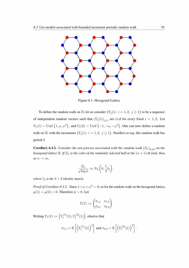
6.3 Urn models associated with bounded increment periodic random walk 91
Figure 6.1: Hexagonal Lattice
To define the random walk on H, let us consider {Yj(i) : i = 1, 2, j ≥ 1} to be a sequence
of independent random vectors such that (Yj(i))j≥1 are i.i.d for every fixed i = 1, 2. Let
Y1(1) ∼ Unif{
1, ω, ω2}, and Y1(2) ∼ Unif
{−1,−ω,−ω2
}. One can now define a random
walk on H, with the increments {Yj(i) : i = 1, 2, j ≥ 1}. Needless to say, this random walk has
period 2.
Corollary 6.3.2. Consider the urn process associated with the random walk (Sn)n≥0 on thehexagonal lattice H. If Zn is the color of the randomly selected ball at the (n+ 1)-th trial, then,as n→∞,
Zn√log n
⇒ N2
(0,
1
2I2),
where I2 is the 2× 2 identity matrix.
Proof of Corollary 6.3.2. Since 1+ω+ω2 = 0, so for the random walk on the hexagonal lattice,µ(1) = µ(2) = 0. Therefore µ = 0. Let
Σ(1) :=
(σ1,1 σ1,2
σ2,1 σ2,2
)
Writing Y1(1) :=(Y
(1)1 (1), Y
(2)1 (1)
), observe that
σ1,1 = E[(Y
(1)1 (1)
)2]
and σ2,2 = E[(Y
(2)1 (1)
)2].

92 Chapter 6: General replacement matrices
Also,σ1,2 = σ2,1 = E
[Y
(1)1 (1)Y
(2)1 (1)
].
Writing ω = Re (ω) + iIm (ω), it is easy to see that
σ1,1 =1
3
(1 + (Re (ω))2 +
(Re(ω2))2)
.
Since Re (ω) = Re(ω2), therefore,
σ1,1 =1
3
(1 + 2 (Re (ω))2
).
Since ω = 12 + i
√3
2 , therefore, this implies σ1,1 = 12 . Similarly, since Im (ω) = −Im
(ω2),
σ2,2 =1
3
((Im (ω))2 +
(Im(ω2))2)
=2
3(Im (ω))2 =
1
2.
Since, Re (ω) = Re(ω2), and Im (ω) = −Im
(ω2),
σ1,2 = σ2,1 =1
3
(Re (ω) Im (ω) + Re
(ω2)Im(ω2))
= 0.
This proves that Σ(1) = 12I2. Similar calculations show that Σ(2) = 1
2I2. This implies thatΣ = 1
2Σ(1) + 12Σ(2) = 1
2I2. This completes the proof.

Bibliography
[1] T. W. Anderson. An introduction to multivariate statistical analysis. Wiley Series in
Probability and Statistics. Wiley-Interscience [John Wiley & Sons], Hoboken, NJ, third
edition, 2003.
[2] Tom M. Apostol. Mathematical analysis. Addison-Wesley Publishing Co., Reading,
Mass.-London-Don Mills, Ont., second edition, 1974.
[3] Krishna B. Athreya and Samuel Karlin. Embedding of urn schemes into continuous time
Markov branching processes and related limit theorems. Ann. Math. Statist., 39:1801–1817,
1968.
[4] A. Bagchi and A. K. Pal. Asymptotic normality in the generalized Polya-Eggenberger
urn model, with an application to computer data structures. SIAM J. Algebraic Discrete
Methods, 6(3):394–405, 1985.
[5] Zhi-Dong Bai and Feifang Hu. Asymptotics in randomized urn models. Ann. Appl. Probab.,
15(1B):914–940, 2005.
[6] Antar Bandyopadhyay and Debleena Thacker. A new approach to Polya urn schemes and
its infinite color generalization. Preprint, 2014.
[7] Antar Bandyopadhyay and Debleena Thacker. Polya urn schemes with infinitely many
colors. (http://arxiv.org/pdf/1303.7374v2.pdf), 2014.
[8] Antar Bandyopadhyay and Debleena Thacker. Rate of convergence and large deviation for
the infinite color Polya urn schemes. Statist. Probab. Lett., 92:232–240, 2014.
93
BIBLIOGRAPHY BIBLIOGRAPHY
[9] Harald Bergstrom. On the central limit theorem in the case of not equally distributed
random variables. Skand. Aktuarietidskr., 32:37–62, 1949.
[10] R. N. Bhattacharya and R. Ranga Rao. Normal approximation and asymptotic expansions.
John Wiley & Sons, New York-London-Sydney, 1976. Wiley Series in Probability and
Mathematical Statistics.
[11] Patrick Billingsley. Probability and measure. Wiley Series in Probability and Mathematical
Statistics. John Wiley & Sons Inc., New York, third edition, 1995. A Wiley-Interscience
Publication.
[12] David Blackwell. Discreteness of Ferguson selections. Ann. Statist., 1:356–358, 1973.
[13] David Blackwell and James B. MacQueen. Ferguson distributions via Polya urn schemes.
Ann. Statist., 1:353–355, 1973.
[14] Arup Bose, Amites Dasgupta, and Krishanu Maulik. Multicolor urn models with reducible
replacement matrices. Bernoulli, 15(1):279–295, 2009.
[15] Arup Bose, Amites Dasgupta, and Krishanu Maulik. Strong laws for balanced triangular
urns. J. Appl. Probab., 46(2):571–584, 2009.
[16] Arijit Chakrabarty. When is a Truncated Heavy Tail Heavy? PhD thesis, Cornell University,
2010.
[17] May-Ru Chen, Shoou-Ren Hsiau, and Ting-Hsin Yang. A new two-urn model. J. Appl.
Probab., 51(2):590–597, 2014.
[18] May-Ru Chen and Markus Kuba. On generalized Polya urn models. J. Appl. Probab.,
50(4):1169–1186, 2013.
[19] Joel E. Cohen. A Model of Simple Competition, volume 41 of Annals of the Computation
Laboratory. Harvard University Press, Cambridge, Massachusetts, second edition, 1966.
[20] Andrea Collevecchio, Codina Cotar, and Marco LiCalzi. On a preferential attachment and
generalized Polya’s urn model. Ann. Appl. Probab., 23(3):1219–1253, 2013.

BIBLIOGRAPHY 95
[21] John B. Conway. Functions of one complex variable, volume 11 of Graduate Texts in
Mathematics. Springer-Verlag, New York, second edition, 1978.
[22] Codina Cotar and Vlada Limic. Attraction time for strongly reinforced walks. Ann. Appl.
Probab., 19(5):1972–2007, 2009.
[23] Edward Crane, Nicholas Georgiou, Stanislav Volkov, Andrew R. Wade, and Robert J.
Waters. The simple harmonic urn. Ann. Probab., 39(6):2119–2177, 2011.
[24] Charles W. Curtis. Linear algebra. Undergraduate Texts in Mathematics. Springer-Verlag,
New York, fourth edition, 1993. An introductory approach.
[25] Amites Dasgupta and Krishanu Maulik. Strong laws for urn models with balanced replace-
ment matrices. Electron. J. Probab., 16:no. 63, 1723–1749, 2011.
[26] Burgess Davis. Reinforced random walk. Probab. Theory Related Fields, 84(2):203–229,
1990.
[27] Amir Dembo and Ofer Zeitouni. Large deviations techniques and applications. Jones and
Bartlett Publishers, Boston, MA, 1993.
[28] Rick Durrett. Probability: theory and examples. Cambridge Series in Statistical and
Probabilistic Mathematics. Cambridge University Press, Cambridge, fourth edition, 2010.
[29] Michael Dutko. Central limit theorems for infinite urn models. Ann. Probab., 17(3):1255–
1263, 1989.
[30] W. J. Ewens. The sampling theory of selectively neutral alleles. Theoret. Population
Biology, 3:87–112; erratum, ibid. 3 (1972), 240; erratum, ibid. 3 (1972), 376, 1972.
[31] Warren J. Ewens. Mathematical population genetics. I, volume 27 of Interdisciplinary
Applied Mathematics. Springer-Verlag, New York, second edition, 2004. Theoretical
introduction.
[32] William Feller. An introduction to probability theory and its applications. Vol. II. Second
edition. John Wiley & Sons, Inc., New York-London-Sydney, 1971.

BIBLIOGRAPHY BIBLIOGRAPHY
[33] Thomas S. Ferguson. A Bayesian analysis of some nonparametric problems. Ann. Statist.,
1:209–230, 1973.
[34] Philippe Flajolet, Philippe Dumas, and Vincent Puyhaubert. Some exactly solvable models
of urn process theory. In Fourth Colloquium on Mathematics and Computer Science
Algorithms, Trees, Combinatorics and Probabilities, Discrete Math. Theor. Comput. Sci.
Proc., AG, pages 59–118. Assoc. Discrete Math. Theor. Comput. Sci., Nancy, 2006.
[35] David A. Freedman. Bernard Friedman’s urn. Ann. Math. Statist, 36:956–970, 1965.
[36] Bernard Friedman. A simple urn model. Comm. Pure Appl. Math., 2:59–70, 1949.
[37] Alexander Gnedin, Ben Hansen, and Jim Pitman. Notes on the occupancy problem with
infinitely many boxes: general asymptotics and power laws. Probab. Surv., 4:146–171,
2007.
[38] Raul Gouet. Strong convergence of proportions in a multicolor Polya urn. J. Appl. Probab.,
34(2):426–435, 1997.
[39] Hsien-Kuei Hwang and Svante Janson. Local limit theorems for finite and infinite urn
models. Ann. Probab., 36(3):992–1022, 2008.
[40] Svante Janson. Functional limit theorems for multitype branching processes and generalized
Polya urns. Stochastic Process. Appl., 110(2):177–245, 2004.
[41] Svante Janson. Limit theorems for triangular urn schemes. Probab. Theory Related Fields,
134(3):417–452, 2006.
[42] Donald E. Knuth. The art of computer programming. Vol. 3. Addison-Wesley, Reading,
MA, 1998. Sorting and searching, Second edition [of MR0445948].
[43] W. Kozakiewicz. On the convergence of sequences of moment generating functions. Ann.
Math. Statistics, 18:61–69, 1947.
[44] Sophie Laruelle and Gilles Pages. Randomized urn models revisited using stochastic
approximation. Ann. Appl. Probab., 23(4):1409–1436, 2013.

BIBLIOGRAPHY 97
[45] Mickael Launay and Vlada Limic. Generalized Interacting Urn Models. available at
http://arxiv.org/abs/1201.3495, 2012.
[46] Gregory F. Lawler and Vlada Limic. Random walk: a modern introduction, volume 123 of
Cambridge Studies in Advanced Mathematics. Cambridge University Press, Cambridge,
2010.
[47] Vlada Limic. Attracting edge property for a class of reinforced random walks. Ann. Probab.,
31(3):1615–1654, 2003.
[48] Vlada Limic and Pierre Tarres. Attracting edge and strongly edge reinforced walks. Ann.
Probab., 35(5):1783–1806, 2007.
[49] Russell Lyons. Strong laws of large numbers for weakly correlated random variables.
Michigan Math. J., 35(3):353–359, 1988.
[50] Hosam M. Mahmoud. Sorting. Wiley-Interscience Series in Discrete Mathematics and
Optimization. Wiley-Interscience, New York, 2000. A distribution theory.
[51] Hosam M. Mahmoud. Polya urn models. Texts in Statistical Science Series. CRC Press,
Boca Raton, FL, 2009.
[52] Shu-teh C. Moy. Extensions of a limit theorem of Everett, Ulam and Harris on multitype
branching processes to a branching process with countably many types. Ann. Math. Statist.,
38:992–999, 1967.
[53] Robin Pemantle. A time-dependent version of Polya’s urn. J. Theoret. Probab., 3(4):627–
637, 1990.
[54] Robin Pemantle. A survey of random processes with reinforcement. Probab. Surv., 4:1–79,
2007.
[55] Robin Pemantle and Stanislav Volkov. Vertex-reinforced random walk on Z has finite range.
Ann. Probab., 27(3):1368–1388, 1999.
BIBLIOGRAPHY BIBLIOGRAPHY
[56] G. Polya. Sur quelques points de la theorie des probabilites. Ann. Inst. H. Poincare,
1(2):117–161, 1930.
[57] Georg Polya. Uber eine Aufgabe der Wahrscheinlichkeitsrechnung betreffend die Irrfahrt
im Straßennetz. Math. Ann., 84(1-2):149–160, 1921.
[58] Eugene Seneta. Non-negative matrices and Markov chains. Springer Series in Statistics.
Springer, New York, 2006. Revised reprint of the second (1981) edition [Springer-Verlag,
New York; MR0719544].
[59] A. N. Shiryayev. Probability, volume 95 of Graduate Texts in Mathematics. Springer-
Verlag, New York, 1984. Translated from the Russian by R. P. Boas.
[60] Robert T. Smythe and Hosam M. Mahmoud. A survey of recursive trees. Teor. Imovır. Mat.
Stat., (51):1–29, 1994.