Geophys. J. Int. (2005) 163, 1087–1111 doi: 10.1111/j.1365-246X.2005.02780.x

GJI

Sei

smol

ogy

Finite-frequency effects in global surface-wave tomography

Ying Zhou,1,∗ F. A. Dahlen,1 Guust Nolet1 and Gabi Laske2

1Department of Geosciences, Princeton University, Princeton, NJ 08544, USA2IGPP, Scripps Institution of Oceanography, University of California San Diego, La Jolla, CA 92093-0225, USA

Accepted 2005 August 8. Received 2005 June 22; in original form 2004 December 30

S U M M A R YWe compare traditional ray-theoretical surface-wave tomography with finite-frequency to-mography, using 3-D Born sensitivity kernels for long-period, fundamental-mode dispersionmeasurements. The 3-D kernels preserve sidelobes beyond the first Fresnel zone, and fullyaccount for the directional dependence of surface-wave scattering, and the effects of time-domain tapering and seismic source radiation. Tomographic inversions of Love and Rayleighphase-delay measurements and synthetic checkerboard tests show that (1) small-scale S-wavevelocity anomalies are better resolved using finite-frequency sensitivity kernels, especiallyin the lowermost upper mantle; (2) the resulting upper-mantle heterogeneities are generallystronger in amplitude than those recovered using ray theory and (3) finite-frequency tomo-graphic models fit long-period dispersion data better than ray-theoretical models of compa-rable roughness. We also examine the reliability of 2-D, phase-velocity sensitivity kernels inglobal surface-wave tomography, and show that phase-velocity kernels based upon a forward-scattering approximation or previously adopted geometrical simplifications do not reliablyaccount for finite-frequency wave-propagation effects. 3-D sensitivity kernels with full con-sideration of directional-dependent seismic scattering are the preferred method of invertinglong-period dispersion data. Finally, we derive 2-D boundary sensitivity kernels for lateralvariations in crustal thickness, and show that finite-frequency crustal effects are not negligiblein long-period surface-wave dispersion studies, especially for paths along continent–oceanboundaries. Unfortunately, we also show that, in global studies, linear perturbation theory isnot sufficiently accurate to make reliable crustal corrections, due to the large difference inthickness between oceanic and continental crust.

Key words: Frechet derivatives, global seismology, sensitivity, surface waves, tomography.

1 I N T RO D U C T I O N

The large-scale seismic structure of the upper mantle has been pro-gressively mapped out by surface-wave tomography during the pastthree decades. Traditional surface-wave tomography is based uponJWKB ray theory, which is valid only if the lateral length scalesof the heterogeneities are larger than the characteristic wavelengthof the seismic waves. Therefore, only the largest-scale structurescan be trusted in traditional long-period surface-wave tomography;furthermore, because structure in the lowermost upper mantle ismainly constrained by surface waves of the longest periods, the spa-tial resolution decreases with depth in ray-theoretical tomography.The limitations of ray theory have received growing attention in re-cent theoretical studies, and sensitivity kernels have been developedto account for finite-frequency effects upon seismic surface-wavepropagation (e.g. Snieder & Nolet 1987; Li & Romanowicz 1995;

∗Now at: Seismological Laboratory, California Institute of Technology,Pasadena, CA 91125, USA. E-mail yingz@gps.caltech.edu

Friederich 1999; Spetzler et al. 2002; Zhou et al. 2004). Yomogida& Aki (1987) were the first to try to account for finite-frequencyeffects in surface-wave phase-velocity tomography, by introducingan ad hoc sensitivity within the first Fresnel zone, scaled expo-nentially to the phase delay between the great-circle ray and thedetoured scattering path. Meier et al. (1997) proposed a two-steptomographic method for surface-wave tomography, in which JWKBwaveform modelling is first used to obtain a preliminary 1-D S-wavevelocity model along each source–receiver path, and the remainingresiduals are then inverted based upon the Born scattering approx-imation. Yoshizawa & Kennett (2004) made use of simplified, 2-D,phase-velocity sensitivity kernels, with a uniform off-path sensi-tivity within the first one-third Fresnel zone, in a surface-wave to-mographic study of Australia. On a global scale, Ritzwoller et al.(2002) have inverted for whole-earth group-velocity maps, using asimplified, uniform-across-the-path version of the 2-D sensitivitykernels developed by Spetzler et al. (2002).

In this paper, we investigate finite-frequency effects in global,long-period, surface-wave, phase-delay tomography, focusing uponthree independent but related topics. First, we compare global

C© 2005 RAS 1087

1088 Y. Zhou et al.

tomographic results based upon traditional surface-wave ray theoryand 3-D, finite-frequency sensitivity kernels. The finite-frequencykernels applied in this study are based upon the single-scattering(Born) approximation, formulated in the framework of surface-wavemode summation (Zhou et al. 2004). The resulting 3-D kernelsfully account for the effects of directional scattering, the effectsof seismogram windowing or tapering, and the effects of seismicsource radiation. The preferred models of S-wave velocity and radialanisotropy in the upper mantle obtained using these finite-frequencysensitivity kernels are documented and discussed in a second paper(Zhou et al. 2005). In this paper, we show that, at the same levelof model roughness, finite-frequency tomography fits a global dis-persion data set better than ray-theoretical tomography, and that,because wave front healing and other diffractional effects are prop-erly accounted for, anomalies with lateral length scales smaller thanthe dominant wavelength are better resolved in finite-frequency to-mography. Second, we point out that surface-wave scattering dueto lateral heterogeneities is directional dependent, and that this de-pendence varies with depth; as a result, phase-velocity maps thatare obtained using approximated or simplified 2-D sensitivity ker-nels may have significant artefacts, and be no more reliable thanthose obtained using traditional ray theory. Third and finally, wedevelop finite-frequency sensitivity kernels for lateral variations incrustal thickness, and discuss the fundamentally intractable problemof making simple and accurate long-period, surface-wave crustalcorrections.

2 T H E O RY

2.1 Ray-theoretical tomography

Traditional surface-wave tomography is based upon JWKB raytheory—a high-frequency approximation. Strictly speaking, ray the-ory is valid only if the angular frequency of the waves is infinitelyhigh. In practice, the surface-wave JWKB approximation is accept-able if the lateral length scale of the 3-D velocity heterogeneity islarge compared to the characteristic wavelength. In this case, mea-sured surface-wave phase delays δφ(ω) can be written as a linearpath integral over the source–receiver great-circle ray:

δφ(ω) = − ω

c(ω)

∫ �

0

δc(ω, l)

c(ω)dl, (2.1)

where ω is the angular frequency, c(ω) is the unperturbed, spherical-earth surface-wave phase velocity, l is the distance along the great-circle ray, and � is the source–receiver epicentral distance. Thefrequency-dependent perturbation in surface-wave phase velocityδc can be expressed in terms of the perturbations in the shear-waveand compressional-wave velocities β and α through relations of theform

δc =∫ R

0

(∂c

∂β

)δβ dr, Love waves, (2.2)

δc =∫ R

0

[ (∂c

∂β

)δβ +

(∂c

∂α

)δα

]dr, Rayleigh waves, (2.3)

where the depth-dependent Frechet derivatives ∂c/∂β and ∂c/∂α

(Dahlen & Tromp 1998, Chapter 11) are functions of radius r andangular frequency ω, and the integration extends from the centre ofthe Earth, r = 0, to the surface, r = R.

2.2 Finite-frequency tomography

In finite-frequency tomography, surface-wave phase delays are sen-sitive not only to heterogeneities along the source–receiver great-circle ray, but also to anomalies that are off the reference ray. Inthis paper, we apply the 3-D, finite-frequency sensitivity kernels forfundamental-mode, surface-wave dispersion measurements devel-oped by Zhou et al. (2004). The measured phase delay at a specificangular frequency ω is written as a volumetric integration over allvelocity heterogeneities in the 3-D earth ⊕, so that eqs (2.1)–(2.3)are replaced by:

δφ(ω) =∫∫∫

⊕Kβ (ω, x)

δβ

β(x) d3x, Love waves (2.4)

δφ(ω) =∫∫∫

⊕

[Kβ (ω, x)

δβ

β(x) + Kα(ω, x)

δα

α(x)

]d3x,

Rayleigh waves, (2.5)

where we have ignored the effects of density perturbations for sim-plicity, based on the following considerations: (1) if we assume man-tle anomalies are dominantly thermal, velocity variations are muchmore significant than density variations; and (2) fundamental-modesurface-wave phase delays are most sensitive to velocity perturba-tions (Zhou et al. 2004).

The 3-D sensitivity kernels K β (ω, x) and K α(ω, x) are computedusing the single scattering approximation; the effects of surface-wave cross-branch mode coupling can be fully taken into accountby a double summation over all surface-wave modes at the fre-quency of interest (Zhou et al. 2004). However, our previous studieshave suggested that the importance of surface-wave cross-branchmode coupling depends upon the desired spatial resolution, andthat mode-coupling effects may be neglected at the current stageof global dispersion tomography, because (1) the spatial resolutionis limited by global path coverage and (2) the number of measure-ments affected by significant surface-wave mode coupling is likelyto be small in hand-picked data sets (Zhou et al. 2004). For thesereasons, we ignore the effects of cross-branch mode coupling inthis tomographic comparison study; this makes the computation ofthe finite-frequency sensitivity kernels very efficient. The factorsthat determine the geometry of the phase-delay kernels have beendiscussed in detail by Zhou et al. (2004); in brief, the cross-pathwidth of the region of significant sensitivity is proportional to thesquare root of the period of the wave. The frequency dependenceof the shear-velocity sensitivity kernel K β (ω, x) is illustrated inFig. 1, where it is seen that 5-mHz Love waves show a cross-pathsensitivity that is

√3 times broader than that of 15-mHz waves. The

3-D sensitivity kernels applied in this study are computed usingthe spherically symmetric reference earth model 1066A (Gilbert &Dziewonski 1975).

3 T O M O G R A P H Y

3.1 Data and model parametrization

To illustrate the importance of accounting for finite-frequency wavepropagation effects in surface-wave tomography, we invert a globaldata set of fundamental-mode Love-wave and Rayleigh-wave dis-persion (Laske & Masters 1996), which include waves that havepropagated along minor arcs (G1, R1) and major arcs (G2, R2), aswell as multiorbits (G3, G4, R3, R4). The phase-delay measurementsare made using a multitaper technique to reduce the bias in spectral

C© 2005 RAS, GJI, 163, 1087–1111

Finite-frequency effects in global surface-wave tomography 1089

Figure 1. 3-D phase-delay sensitivity kernel K β for (a) 15-mHz and (b) 5-mHz fundamental-mode Love waves. Map views of the 15- and 5-mHz sensitivitykernels K β are plotted at 80 and 250 km depth, respectively (dotted lines in the cross-sections). The cross-path variations in sensitivity at those depths are plottedbelow the cross-sections. The seismic source is strike-slip, with Love-wave radiation symmetric about the source–receiver great-circle path (see beachball).The epicentral distance is 80◦. Letters S, R, A and B denote the source, receiver and endpoints of the cross-section, respectively. Surface-wave mode couplingeffects are ignored.

estimates (Laske & Masters 1996). This data set includes a totalof ∼12 000 wave trains, including both Love waves and Rayleighwaves. The frequencies of the dispersion measurements range from5 to 15 mHz, with an interval of 1 mHz. All measurements are resid-uals with respect to model 1066A (Gilbert & Dziewonski 1975).

We parametrize the surface of the Earth using a set of sphericaltriangular grid points (Baumgardner & Frederickson 1985). The tri-angulation starts with 20 equal spherical triangles, and is iterativelyrefined by connecting the midpoint of the three sides of each trian-gle (Fig. 2). The spherical triangles used in this study are 16-fold,with 2562 vertexes and 5120 triangles. The lateral spacing betweenneighbouring grid points is 4.3◦ ± 0.3◦. We assume that the seis-mic velocity within any spherical triangle can be approximated bylinear spatial interpolations through the velocities at the three ver-texes. In the radial (depth) direction, the uppermost 580 km of theupper mantle is parametrized using nine grid points, with a nominalgrid spacing of 60 km in the uppermost 400 km; velocity pertur-bations are interpolated linearly between neighbouring depth gridpoints.

3.2 The inverse problem

We invert for the fractional S-wave velocity perturbations δβ/β

at the 2562 × 9 = 23 058 grid points. The P-wave velocity per-turbations are scaled to the S-wave velocity perturbations using therelation δα/α = 0.5 (δβ/β), adapted from laboratory measurementsbased on petrological models of the upper mantle (Montagner &Anderson 1989). We have experimented with scaling parameters inthe range 0 ≤ (δα/α)/(δβ/β) ≤ 1, and find that the tomographicresults do not vary significantly. The discrete forms of both ray-theoretical tomography, eqs (2.1)–(2.3), and finite-frequency tomog-raphy, eqs (2.4)–(2.5), can be written in the canonical form

Am = b, (3.1)

where A is the sensitivity kernel matrix, m is the vector of unknownparameters δβ/β, and b is the phase-delay data vector. To computethe finite-frequency kernel matrix A, the numerical integrations ineqs (2.4)–(2.5) are carried out with spatial samplings that are fineenough to avoid possible aliasing in the sensitivity kernels; all of

C© 2005 RAS, GJI, 163, 1087–1111

1090 Y. Zhou et al.

Figure 2. Icosahedral spherical triangulation (Baumgardner & Frederickson 1985). (a) The starting twenty equal spherical triangles. (b) The refined finalspherical triangles after a 16-fold triangulation; the spatial separation of neighbouring grid points is 4.3◦ ± 0.3◦.

Figure 3. Diagonal elements of the matrix products ATA in ray-theoretical (left) and finite-frequency (right) tomography, plotted at a depth of 180 km. In thetop two maps, (a) and (b), the matrix A includes sensitivities of Love waves with frequencies from 5 to 15 mHz and wave trains G1, G2, G3 and G4. In thebottom two maps, (c) and (d), the matrix A includes sensitivities of Rayleigh waves with frequencies from 5 to 15 mHz and wave trains R1, R2, R3 and R4.

the sidebands as well as spatial sensitivity variations within thefirst Fresnel zone are fully accounted for in the computation. Thediagonal elements of the ray-theoretical and finite-frequency matrixproducts ATA, a measure of the spatial coverage of the data, areplotted in Fig. 3. Naively, we might expect the matrix density ATAto be more uniform in finite-frequency tomography, because of theoff-ray spreading of the sensitivity. In practice, since the majority ofthe great-circle ray paths are not near the maximum of the outgoingsource radiation, the finite-frequency spatial coverage is comparableto that of ray theory.

Due to limited and uneven global path coverage, as well as con-tamination of the data by noise, the tomographic equation is under-

determined, and the inverse matrix (ATA)−1 is singular or ill-posed.In this study, we apply a Laplacian smoothing to regularize the least-squares inverse problem, (Am − b)T(Am − b) = minimum, and wesimultaneously invert for perturbations to the source origin timest = (. . . , tk , . . .), so that the tomographic problem becomes

χ 2 + ε ||Sm||2 + εt ||t||2 = minimum,

where χ2 =N∑

i=1

(Ai j m j + Hiktk − bi

σi

)2

. (3.2)

The quantity N is the total number of phase-delay measurements,

and χ 2 is the data misfit function, with σ i being the observational

C© 2005 RAS, GJI, 163, 1087–1111

Finite-frequency effects in global surface-wave tomography 1091

error associated with the ith measurement bi. The product Hiktk rep-resents the phase delay in the ith observation due to a shift tk in theorigin time of the kth earthquake. Summation over the model pa-rameter index j and the earthquake index k in eq. (3.2) is understood.The quantity

||Sm|| ≈(∫ ∫ ∫

⊕|∇2(δβ/β)|2 d3x

)1/2

(3.3)

is an approximate, discretized measure of the root-mean-square(rms) Laplacian of the fractional velocity perturbation. The smooth-ing parameter ε governs the trade-off between the model Laplacianof the inverted model and the misfit to the data; We choose anorigin-time damping parameter ε t such that the perturbations tk arenot greater than ±4 s; because the surface waves used in this studyare long-period (67–200 s), the differences between tomographicmodels inverted with and without origin-time corrections are neg-ligible. The sparse linear tomographic problem, eq. (3.2), is solvedusing the LSQR algorithm (Paige & Saunders 1982), iterated un-til full convergence. If the observations are contaminated by noisewith a Gaussian distribution, the data misfit χ2 of the recoveredearth model should approach the number of observations, that is,χ 2/N = 1.

We apply crustal corrections to the global phase-delay data set,based on a global crust model, CRUST2.0 (Laske et al. 2001), whichspecifies a seven-layer crust in each 2◦ by 2◦ grid. Maps of the lo-cal phase-delay corrections due to the CRUST2.0 crustal variationsare computed at each of the discrete frequencies of measurement,

Figure 4. Misfit versus roughness trade-off curves for finite-frequency (FF) and ray-theoretical (RT) tomography. In (a) and (b) both the Love and Rayleigh‘no-smoothing’ (ε = 0) finite-frequency models have roughness ||Sm||/||m|| ≈ 0.11; the corresponding ray-theoretical ‘no-smoothing’ models are out of thescale, with roughnesses ||Sm||/||m|| ≈ 0.52 and ||Sm||/||m|| ≈ 0.60, for Love and Rayleigh waves, respectively. Plots (c) and (d) show blowups of the regionsoutlined by the dotted boxes in (a) and (b). The black stars indicate the chosen ‘optimal’ finite-frequency models discussed in the paper; the white stars areray-theoretical models with the same roughness ||Sm||/||m||, and the grey stars are ray-theoretical models with the same misfit χ2/N . Map views of the starredtomographic models are plotted in Figs 5–8.

5–15 mHz, and ray-theoretical crustal corrections are then calcu-lated for each phase-delay observation by integration along the raypath. In Section 6, we show that finite-frequency crustal effects uponlong-period surface waves are not negligible; however, boundarytopography sensitivity kernels that are based upon the Born approx-imation are not sufficiently accurate to account for the large globalvariations in Moho depth. The observational errors σ i in eq. (3.2)are estimated from phase-delay measurements of closely spacedearthquake pairs, based upon the assumption that the surface wavesexcited by these repeating earthquakes sample approximately thesame region of the upper mantle, and therefore should experiencenearly equal phase delays. The rms of the estimated observationalerrors is about 45–75 per cent of the rms of the measured phasedelays (Zhou et al. 2005).

4 F I N I T E - F R E Q U E N C Y E F F E C T SI N 3 - D T O M O G R A P H Y

In this section, we compare S-wave velocity models obtained byinversion of the same phase-delay measurements using both finite-frequency and ray-theoretical kernel matrices A. Fig. 4 shows thetrade-offs between the model roughness (normalized model Lapla-cian) ||Sm||/||m|| and the data misfit χ 2/N , where the quantity||m|| = ||m||/√N is the rms of the velocity perturbation δβ/β.The roughness of the model is insensitive to the perturbation norm||m||. In both ray-theoretical and finite-frequency tomography, thenormalized data misfit χ2/N is greater than one, which indicates

C© 2005 RAS, GJI, 163, 1087–1111

1092 Y. Zhou et al.

that the errors assigned to the phase-delay measurements are under-estimated. In tomographic practice, it is often difficult to estimate theactual error in the data; furthermore, the assumption that the noiseis Gaussian may be invalid. For these reasons, we do not rescale theestimated errors in the data to force χ2/N = 1, but instead acceptmodels with misfits χ 2/N slightly greater than one.

4.1 3-D model comparison: kernels versus rays

The ‘optimal’ finite-frequency tomographic model discussed in thispaper is chosen to be near the lower left corner of the χ2/N versus||Sm||/||m|| trade-off curve, where small reductions in the misfitto the data begin to require large increases in the roughness of themodel. We compare the ‘optimal’ finite-frequency model (blackstars in Fig. 4) with two different ray-theoretical models, one chosento have the same roughness ||Sm||/||m|| (white stars) and the otherto have the same data misfit χ 2/N (grey stars). Map views of thevelocity models obtained by independent inversions of the Love-wave and the Rayleigh-wave data are plotted in Figs 5–8.

The poor agreement between the models obtained by invertingLove and Rayleigh phase delays confirms that there is strong ra-dial anisotropy in the upper mantle. A joint Love–Rayleigh inver-sion using isotropic kernels K β and K α results in a poor data fit,

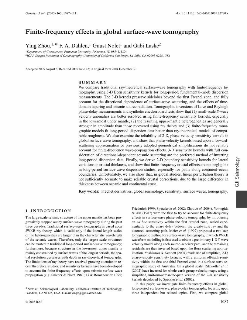
Figure 5. S-wave velocity model obtained by (a) ray-theoretical tomography and (b) finite-frequency tomography. The two models have the same modelroughness, ||Sm||/||m|| ≈ 0.016, with different values of χ2/N , as indicated. The velocity perturbations are with respect to model 1066A, with the sphericalaverage in each map removed for better illustration. Models are inverted using Love-wave phase delays, and are plotted at depths of 120, 250 and 390 km.Hotspots are indicated by red triangles, and the age contours (blue) indicate 10 Myr old seafloor. The two models agree in their large-scale structure; however,anomalies in the finite-frequency tomographic model are stronger in amplitude, with small-scale features better resolved.

with systematic Love–Rayleigh discrepancies, and, only the largest-scale common structures are well constrained. The inability of asingle isotropic S-wave velocity model to provide a satisfactory fitto both Love and Rayleigh waves has been widely reported in pre-vious surface-wave studies (e.g. Anderson 1961; Aki & Kaminuma1963). In this paper we confine ourselves to independent inversionsof Love and Rayleigh data, and focus upon the comparison betweentraditional surface-wave ray theory and finite-frequency sensitiv-ity kernels. In both the Love-wave and Rayleigh-wave inversions,finite-frequency tomographic models exhibit a better fit to the datathan ray-theoretical models, at the same level of model roughness||Sm||/||m|| (this is most evident in the magnified trade-off curvesin Fig. 4).

Figs 5 and 6 show map views of δβ/β at depths of 120, 250 and390 km, obtained by inverting Love-wave phase delays. The ray-theoretical model in Fig. 5 has the same roughness, ||Sm||/||m|| ≈0.016, as the ‘optimal’ finite-frequency model, whereas the model inFig. 6 has the same data misfit, χ2/N ≈ 1.51. The long-wavelengthfeatures in the finite-frequency and ray-theoretical Love-wavemodels are in good agreement; in particular, all three models arecharacterized by slow anomalies beneath midocean ridges and fastanomalies beneath continental cratons. A number of small-scalevelocity anomalies that are weak or absent in the ray-theoretical

C© 2005 RAS, GJI, 163, 1087–1111

Finite-frequency effects in global surface-wave tomography 1093

Figure 6. Same as Fig. 5, expect that the two models now fit the data equally well, χ2/N ≈ 1.51, with different values of the model roughness ||Sm||/||m||,as indicated. The S-wave velocity anomalies are stronger in the finite-frequency model, especially in the deeper part of the upper mantle.

models can be more easily identified using finite-frequency to-mography; notable examples are the slow anomalies at 390 kmdepth beneath the southern Pacific superswell, the Red Sea, theBasin and Range Province, and the North Mid-Atlantic Ocean.Figs 7–8 show map-view comparisons of the equal-roughness,||Sm||/||m|| ≈ 0.022, and equal-misfit, χ2/N ≈ 1.22, modelsobtained by inverting Rayleigh-wave phase delays. The essentialobservations are similar to those in the Love-wave comparisons.In the central Pacific, the differences between the ray-theoreticaland finite-frequency Rayleigh-wave models are significant in themiddle portion of the upper mantle; the western Pacific subduc-tion zones are better resolved in the finite-frequency model, par-ticularly at 390 km depth. Geographically, there does not appearto be any correlation between the ray-path density (Fig. 3) and thedifferences between the ray-theoretical and finite-frequency tomo-graphic velocity models. For example, the models differ signifi-cantly in the southern Pacific Ocean, where the ray-path coverageis relatively poor; on the other hand, there are also large differencesbeneath western North America, where the coverage is relativelydense.

In both the Love-wave and Rayleigh-wave comparisons, the finite-frequency model has stronger small-scale anomalies than eitherthe equal-roughness or the equal-misfit ray-theoretical model. Thisis mainly because the 3-D sensitivity kernels applied in finite-

frequency tomography account for the effects of wave front healing,that is, a diverging or converging surface wave heals as it propagatesbeyond the causative fast or slow velocity anomaly. As a result, thephase delays observed at seismic stations are generally smaller thanthe original phase delay incurred by a wave upon passage throughan anomaly. In ray theory, wave front healing effects are not ac-counted for, and as a result, the recovered anomalies are generallyweaker in amplitude. Analogous finite-frequency effects in body-wave tomography have been noted by Montelli et al. (2004) andHung et al. (2004). The main result is the same for surface wavesas for body waves: finite-frequency tomography generally recoversstronger small-scale anomalies than ray theory.

The mean velocity perturbation at every depth has been sub-tracted, so that the lateral variations in all of the maps 5–8 averageto zero. The updated, spherically averaged velocity profiles β(r ) ob-tained by finite-frequency tomography and ray-theoretical tomogra-phy are compared in Fig. 9. The degree-zero profiles β(r ) are seento be almost identical, so maps in Figs 5–8 can be properly com-pared. The rms velocity perturbations 〈(δβ/β)2〉1/2 are also plottedversus depth in Fig. 9. Regardless of whether the ray-theoreticalmodel is constrained to have the same roughness, ||Sm||/||m||, orthe same data misfit, χ 2/N , the rms velocity anomalies in the ‘op-timal’ finite-frequency model are larger at all depths, by as much as30 per cent.

C© 2005 RAS, GJI, 163, 1087–1111

1094 Y. Zhou et al.

Figure 7. Same as Fig. 5, except for Rayleigh waves rather than Love waves. The two models have the same roughness ||Sm||/||m|| ≈ 0.022.

4.2 Spectral power and model correlations

To further investigate the enhancement of small-scale features infinite-frequency tomography, we decompose the S-wave velocitymaps into spherical harmonics. We use the real spherical harmonicconvention of Dahlen & Tromp (1998, Section B.8), in which a real,zero-mean, function of geographical position ψ(θ , φ) is expandedin the form

ψ(θ, φ) =∞∑

l=1

[al0 Xl0(θ ) +

√2

l∑m=1

Xlm(θ )(alm cos mφ + blm sin mφ)

], (4.1)

where the orthonormality relation governing the real colatitudinalharmonics Xlm (θ ) is∫ π

0Xlm(θ )Xl ′′ (θ ) sin θdθ = 1

2πδll ′ . (4.2)

The power per degree l and per unit area is defined by

Pl = 1

2l + 1

[a2

l0 +l∑

m=1

(a2

lm + b2lm

)], (4.3)

and the correlation coefficient Cl is defined by

Cl =al0a′

l0 +l∑

m=1(alma′

lm + blmb′lm)√

l∑m=1

(a2

lm + b2lm

)√ l∑m=1

(a′2

lm + b′2lm

) , (4.4)

where alm, blm and a′lm, b′

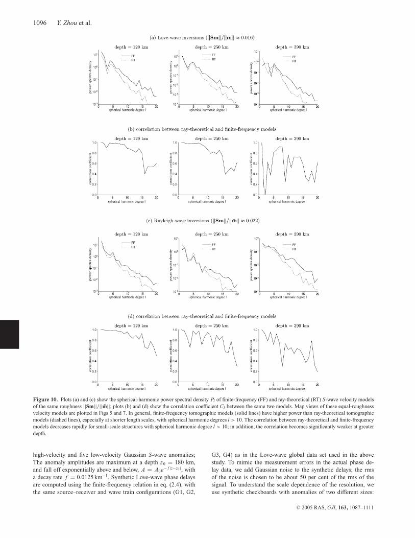
lm are the real spherical expansion har-monic coefficients of the two velocity maps being compared. Thepower spectral density Pl of the velocity perturbations δβ/β, aswell as the finite-frequency versus ray-theoretical correlation co-efficients Cl are plotted versus spherical harmonic degree l, at thethree depths 120, 250 and 390 km, in Figs 10 and 11. The spec-tral comparisons confirm that the imaged velocity anomalies arein general ‘stronger’ in finite-frequency tomography. The correla-tion Cl between the ray-theoretical and finite-frequency models de-creases rapidly with increasing spherical harmonic degree above l ≈10; in addition, the correlation is markedly weaker at greater depth(390 km) in both the Love-wave and the Rayleigh-wave inversions.These are both expected results, inasmuch as finite-frequency effectsbecome more significant with increasing wavelength, and deep-seated structures are mainly constrained by long-period surfacewaves. In Fig. 10, where the two models have the same roughness||Sm||/||m||, there is a clear and growing excess of high-degreepower in the finite-frequency model; this scale dependence of thedifference in Pl versus l is not as pronounced in Fig. 11, where thetwo models fit the phase-delay data equally well but have differentroughness.

4.3 Checkboard tests: scale-dependent resolution

In this subsection we investigate the resolution and fidelity ofray-theoretical and finite-frequency tomography using syntheticcheckboard tests. The input checkboards consist of five

C© 2005 RAS, GJI, 163, 1087–1111

Finite-frequency effects in global surface-wave tomography 1095

Figure 8. Same as Fig. 6, except for Rayleigh waves rather than Love waves. The finite-frequency and ray-theoretical models have the same data misfit,χ2/N ≈ 1.22. Small-scale structures differ significantly between the two models throughout the upper mantle.

Figure 9. Depth variation of the spherically averaged S-wave velocity β and the rms variation of the 3-D perturbations, 〈(δβ/β)2〉1/2, for both finite-frequency(FF) and ray-theoretical (RT) tomography.

C© 2005 RAS, GJI, 163, 1087–1111

1096 Y. Zhou et al.

Figure 10. Plots (a) and (c) show the spherical-harmonic power spectral density Pl of finite-frequency (FF) and ray-theoretical (RT) S-wave velocity modelsof the same roughness ||Sm||/||m||; plots (b) and (d) show the correlation coefficient Cl between the same two models. Map views of these equal-roughnessvelocity models are plotted in Figs 5 and 7. In general, finite-frequency tomographic models (solid lines) have higher power than ray-theoretical tomographicmodels (dashed lines), especially at shorter length scales, with spherical harmonic degrees l > 10. The correlation between ray-theoretical and finite-frequencymodels decreases rapidly for small-scale structures with spherical harmonic degree l > 10; in addition, the correlation becomes significantly weaker at greaterdepth.

high-velocity and five low-velocity Gaussian S-wave anomalies;The anomaly amplitudes are maximum at a depth z0 = 180 km,and fall off exponentially above and below, A = A0e− f |z−z0|, witha decay rate f = 0.0125 km−1. Synthetic Love-wave phase delaysare computed using the finite-frequency relation in eq. (2.4), withthe same source–receiver and wave train configurations (G1, G2,

G3, G4) as in the Love-wave global data set used in the abovestudy. To mimic the measurement errors in the actual phase de-lay data, we add Gaussian noise to the synthetic delays; the rmsof the noise is chosen to be about 50 per cent of the rms of thesignal. To understand the scale dependence of the resolution, weuse synthetic checkboards with anomalies of two different sizes:

C© 2005 RAS, GJI, 163, 1087–1111

Finite-frequency effects in global surface-wave tomography 1097

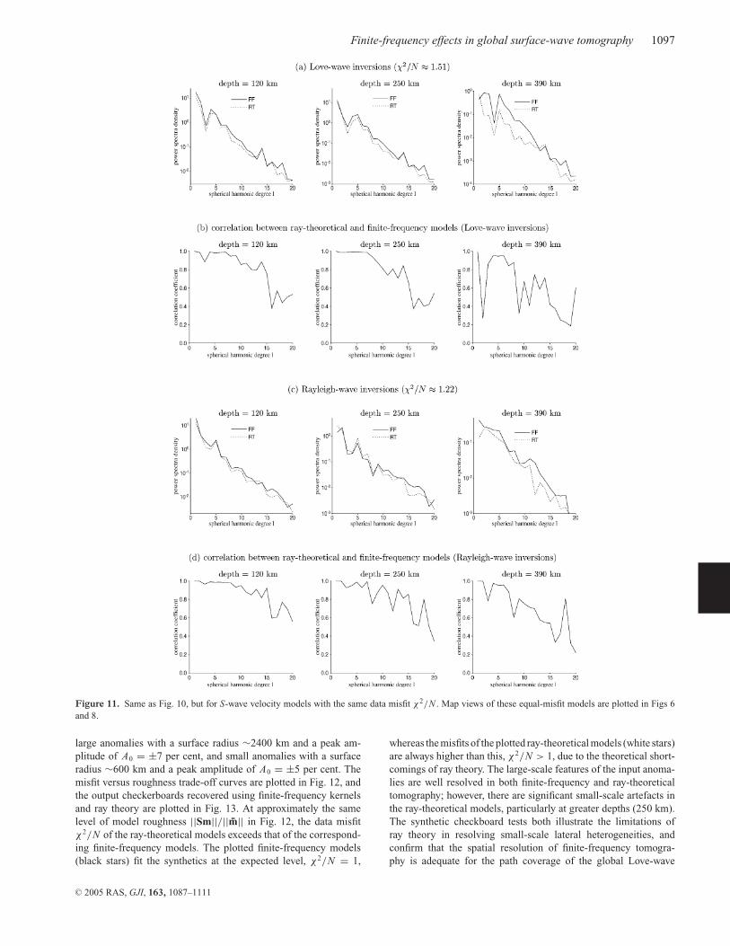
Figure 11. Same as Fig. 10, but for S-wave velocity models with the same data misfit χ2/N . Map views of these equal-misfit models are plotted in Figs 6and 8.

large anomalies with a surface radius ∼2400 km and a peak am-plitude of A0 = ±7 per cent, and small anomalies with a surfaceradius ∼600 km and a peak amplitude of A0 = ±5 per cent. Themisfit versus roughness trade-off curves are plotted in Fig. 12, andthe output checkerboards recovered using finite-frequency kernelsand ray theory are plotted in Fig. 13. At approximately the samelevel of model roughness ||Sm||/||m|| in Fig. 12, the data misfitχ 2/N of the ray-theoretical models exceeds that of the correspond-ing finite-frequency models. The plotted finite-frequency models(black stars) fit the synthetics at the expected level, χ2/N = 1,

whereas the misfits of the plotted ray-theoretical models (white stars)are always higher than this, χ2/N > 1, due to the theoretical short-comings of ray theory. The large-scale features of the input anoma-lies are well resolved in both finite-frequency and ray-theoreticaltomography; however, there are significant small-scale artefacts inthe ray-theoretical models, particularly at greater depths (250 km).The synthetic checkboard tests both illustrate the limitations ofray theory in resolving small-scale lateral heterogeneities, andconfirm that the spatial resolution of finite-frequency tomogra-phy is adequate for the path coverage of the global Love-wave

C© 2005 RAS, GJI, 163, 1087–1111

1098 Y. Zhou et al.

Figure 12. Trade-off curves of the checkboard tests for (a) large and (b) small anomalies. The ‘optimal’ models, shown as stars in the trade-off curves,are plotted in Fig. 13. Ray-theoretical inversions always show data misfit larger than χ2/N = 1, due to the theoretical errors inherent in ray theory. Thefinite-frequency ‘no-smoothing’ (ε = 0) models have roughnesses ||Sm||/||m|| equal to 0.06 and 0.07 for (a) large and (b) small anomalies, respectively; theray-theoretical “no-smoothing” models have roughnesses ||Sm||/||m|| equal to 0.28 and 0.11 for large and small anomalies, respectively.

Figure 13. Checkboard resolution tests of finite-frequency and ray-theoretical surface-wave tomography. (a) The checkboard anomalies are smooth Gaussiananomalies, with a peak amplitude of ±7 per cent at 180 km, and a radius ∼2400 km. The amplitude of the anomalies decreases both upward and downward,with an exponential decay rate f = 0.0125 km−1. (b) The peak amplitude of the Gaussian anomalies is ±5 per cent at 180 km, and the radius is ∼600 km. Thesynthetic Love-wave phase delays are computed using 3-D sensitivity kernels, with the same path and frequency configurations as in the global data set used inthis paper. The output models are all inverted with 50 per cent synthetic Gaussian noise. Ray-theoretical tomography recovers the large-scale structure of theinput model, but it poorly resolves small-scale anomalies, especially at deep depth (250 km). The trade-off curves are plotted in Fig. 12.

C© 2005 RAS, GJI, 163, 1087–1111

Finite-frequency effects in global surface-wave tomography 1099

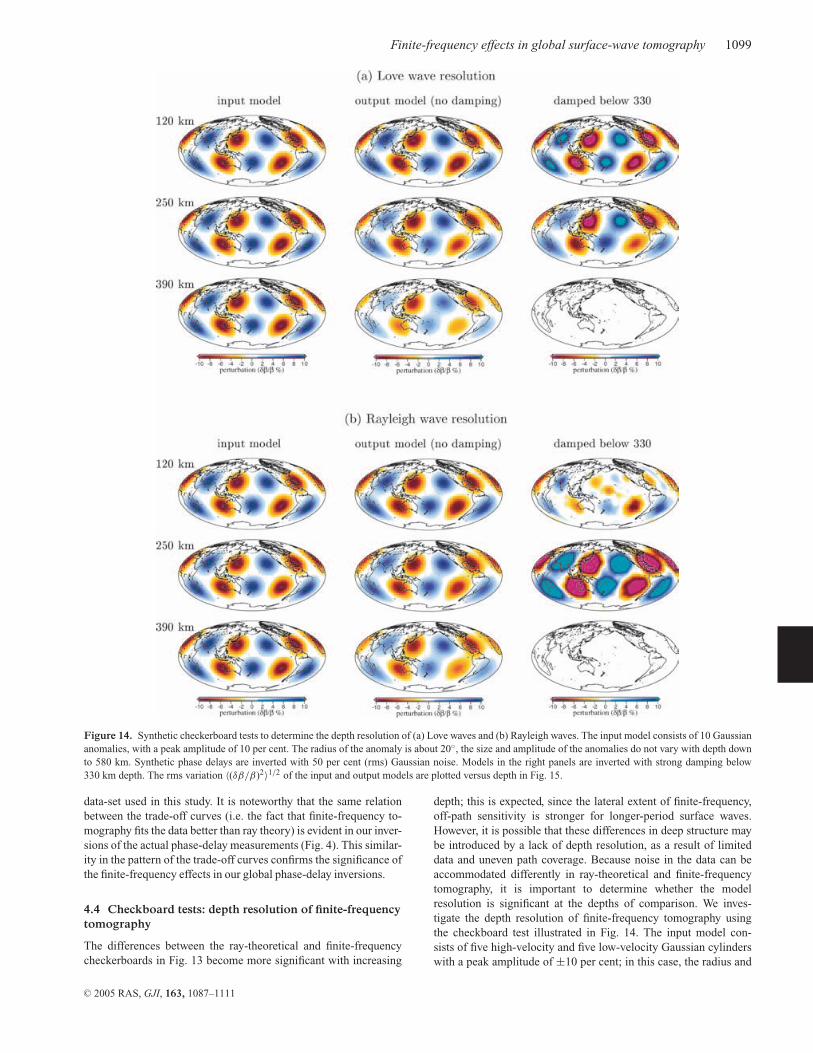
Figure 14. Synthetic checkerboard tests to determine the depth resolution of (a) Love waves and (b) Rayleigh waves. The input model consists of 10 Gaussiananomalies, with a peak amplitude of 10 per cent. The radius of the anomaly is about 20◦, the size and amplitude of the anomalies do not vary with depth downto 580 km. Synthetic phase delays are inverted with 50 per cent (rms) Gaussian noise. Models in the right panels are inverted with strong damping below330 km depth. The rms variation 〈(δβ/β)2〉1/2 of the input and output models are plotted versus depth in Fig. 15.

data-set used in this study. It is noteworthy that the same relationbetween the trade-off curves (i.e. the fact that finite-frequency to-mography fits the data better than ray theory) is evident in our inver-sions of the actual phase-delay measurements (Fig. 4). This similar-ity in the pattern of the trade-off curves confirms the significance ofthe finite-frequency effects in our global phase-delay inversions.

4.4 Checkboard tests: depth resolution of finite-frequencytomography

The differences between the ray-theoretical and finite-frequencycheckerboards in Fig. 13 become more significant with increasing

depth; this is expected, since the lateral extent of finite-frequency,off-path sensitivity is stronger for longer-period surface waves.However, it is possible that these differences in deep structure maybe introduced by a lack of depth resolution, as a result of limiteddata and uneven path coverage. Because noise in the data can beaccommodated differently in ray-theoretical and finite-frequencytomography, it is important to determine whether the modelresolution is significant at the depths of comparison. We inves-tigate the depth resolution of finite-frequency tomography usingthe checkboard test illustrated in Fig. 14. The input model con-sists of five high-velocity and five low-velocity Gaussian cylinderswith a peak amplitude of ±10 per cent; in this case, the radius and

C© 2005 RAS, GJI, 163, 1087–1111

1100 Y. Zhou et al.

Figure 15. Depth resolution of the fundamental-mode Love waves and Rayleigh waves used in this study. Plots (a) and (b) show the rms depth profiles〈(δβ/β)2〉1/2 of the Gaussian checkerboard models in Fig. 14(a). Plots (c) and (d) show the corresponding depth profiles of the models in Fig. 14(b). In (b) and(d) strong damping is applied to structures deeper than 330 km in the inversion; this results in large errors in the output model at shallow depths. The results ofthese resolution tests indicate both that the Love-wave and Rayleigh-wave data used in the paper have significant sensitivity to structures below 330 km, andthat Rayleigh waves have stronger sensitivity at below 330 km depth than Love waves.

amplitude of the anomalies are constant down to a depth of 580 km.As before, to make the inversion more realistic, we invert syn-thetic Love-wave and Rayleigh-wave phase delays contaminated by50 per cent (rms) random noise. The output models exhibit roughlyGaussian cylinders reasonably well-recovered geographically at alldepths; as expected, the recovered anomalies are weaker at greaterdepths because of the reduced data sensitivity (Fig. 14). To testthe model resolution in the lowermost upper mantle, we performadditional inversions, in which strong norm damping is applied toanomalies deeper than 330 km. The resulting velocity models showsignificant artefacts at shallow depths, especially in the Rayleigh-wave inversion. All of the output models in Fig. 14 fit the syn-thetic Love-wave phase-delay data equally well (χ2/N = 1). Therms variation of the recovered models is plotted versus depth inFig. 15. This final series of checkboard tests indicates that modelresolution below 330 km is less than that at shallower depths; nev-ertheless, the sensitivity in the lowermost upper mantle is suffi-cient that reliable model comparisons may be made even at thosedepths.

5 F I N I T E - F R E Q U E N C Y E F F E C T SI N P H A S E - V E L O C I T Y M A P S

In traditional, ray-theoretical, surface-wave tomography, dispersiondata are often used to make 2-D maps of the fractional perturba-tion in phase velocity, δc/c, at discrete frequencies (e.g. Trampert& Woodhouse 1995; Laske & Masters 1996; Ekstrom et al. 1997).Phase-velocity perturbations at high frequencies are associated withS-wave velocity perturbations at shallow depths, whereas perturba-tions at low frequencies are influenced by velocity anomalies downto greater depth. The intermediate 2-D phase velocity maps arethen used as input ‘data’ to constrain 3-D S-wave velocity anoma-lies, using depth-dependent Frechet kernels ∂c(ω)/∂β(r ). It hasbeen pointed out that in the presence of lateral heterogeneities,surface-wave phase-velocity measurements can be contaminated byinterference from scattered arrivals (Wielandt 1993). Whenever thelength scale of lateral heterogeneities is comparable to the wave-length of the surface waves, finite-frequency effects must be takeninto account. 2-D sensitivity kernels for the local phase-velocity

C© 2005 RAS, GJI, 163, 1087–1111

Finite-frequency effects in global surface-wave tomography 1101

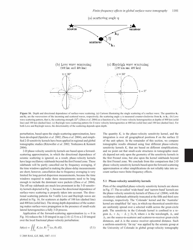
Figure 16. Depth and directional dependence of surface-wave scattering. (a) Cartoon illustrating the single scattering of a surface wave. The quantities k1

and k2 are the wavevectors of the incoming and scattered waves, respectively; the scattering angle η is measured counter-clockwise from k1 to k2. (b) Lovewave scattering pattern, that is, the scattering strength |�β | (Zhou et al. 2004) as a function of η, for S-wave velocity heterogeneities at depths of 400 km (solidline) and 100 km (dashed line). (c) Rayleigh wave scattering pattern for S-wave velocity heterogeneities at 400 km (solid line) and 100 km (dashed line). Forboth Love and Rayleigh waves, the directionality of the scattering depends upon depth.

perturbation, based upon the single-scattering approximation, havebeen developed (Spetzler et al. 2002; Zhou et al. 2004), and simpli-fied 2-D sensitivity kernels have been applied in regional and globaltomographic studies (Ritzwoller et al. 2002; Yoshizawa & Kennett2004).

2-D phase-velocity sensitivity kernels are based upon a forward-scattering approximation, in which the directional dependence ofseismic scattering is ignored; as a result, phase-velocity kernelshave large oscillatory sidebands beyond the first Fresnel zone. Thesesidebands will be partly cancelled out by frequency averaging, ifthe time windows applied in making the phase-delay measurementsare short; however, cancellation due to frequency averaging is verylimited for long-period dispersion measurements, because the timewindows required to make these measurements need to be longenough to include the dominant wave packets (Zhou et al. 2004).The off-ray sidebands are much less prominent in the 3-D sensitiv-ity kernels depicted in Fig. 1, because the directional dependence ofsurface-wave scattering is properly taken into account. The direc-tional scattering patterns for 5-mHz Love and Rayleigh waves areplotted in Fig. 16, for scatterers at depths of 100 km (dashed line)and 400 km (solid line). The strong depth dependence of the scatter-ing makes surface-wave propagation in the presence of small-scalelateral heterogeneities a fully 3-D process.

Application of the forward-scattering approximation (η = 0 inFig. 16) reduces the 3-D integral in eqs (2.4)–(2.5) to a 2-D integralover the local fractional phase-velocity perturbation:

δφ(ω) =∫∫

�

Kc(ω, r)δc

c(ω, r) d�. (5.1)

The quantity Kc is the phase-velocity sensitivity kernel, and theintegration is over all geographical positions r on the surface �

of the unit sphere. In the remainder of this section, we comparetomographic results obtained using four different phase-velocitysensitivity kernels Kc that are based on different simplifications,and we point out that small-scale structures in tomographic mod-els depend not only upon the geometry of the sensitivity kernels inthe first Fresnel zone, but also upon the kernel sidebands beyondthe first Fresnel zone. We conclude from this comparison that 2-Dphase-velocity sensitivity kernels based upon the forward-scatteringapproximation or other simplifications do not reliably take into ac-count surface-wave finite-frequency effects.

5.1 Phase-velocity sensitivity kernels

Plots of the simplified phase-velocity sensitivity kernels are shownin Fig. 17. The so-called ‘wide-band’ and ‘narrow-band’ kernels arethe phase-velocity sensitivity kernels of Zhou et al. (2004), with theoscillatory sidebands arbitrarily truncated at the fifth and third zerocrossings, respectively. The ‘Colorado’ kernel and the ‘Australia’kernel are simplified ‘fat’ rays, in which ray-theoretical sensitivitiesare uniformly spread over a selected width across the great-circlepath. The sensitivity in the Colorado kernel is confined to a re-gion �1 + �2 − � ≤ 3λ/8, where λ is the wavelength, �1 and�2 are the source-to-scatterer and scatterer-to-receiver great-circledistances, and � is the source–receiver epicentral distance. Sucha uniform-sensitivity ‘fat ray’ was applied by the seismic group atthe University of Colorado in global group-velocity tomography

C© 2005 RAS, GJI, 163, 1087–1111

1102 Y. Zhou et al.

Figure 17. Examples of 2-D phase-velocity sensitivity kernel Kc. Green star and triangle denote the source and receiver, respectively. The wide-band andnarrow-band sensitivity kernels are computed using the expressions given by Zhou et al. (2004), with the sidebands truncated at the fifth and third zero-crossing,respectively. The Colorado kernel, in which the cross-path sensitivity is constant within the region �1 + �2 − � ≤ 3λ/8 is adapted from Ritzwoller et al.(2002). The Australia kernel is that proposed to Yoshizawa & Kennett (2002), with a cross-path width �1 + �2 − � ≤ λ/18.

(Ritzwoller et al. 2002). The cross-path width of the Australia ker-nel is one-third of the first Fresnel zone, that is, �1 + �2 − � ≤λ/18 (Yoshizawa & Kennett 2002). Such a narrower ‘fat ray’ hasbeen applied in Australian regional phase-velocity tomography byYoshizawa & Kennett (2004).

5.2 Phase-velocity kernel comparisons

Love-wave phase-velocity maps at 5 and 15 mHz obtained usingtraditional ray theory, eq. (2.1), as well as the four different phase-velocity sensitivity kernels in eq. (5.1), are plotted in Fig. 18. All ofthe recovered maps fit the data equally well (χ 2/N ≈ 2). We attributeour inability to fit the data better than this to be due to the severity ofthe approximations used in the computation of the phase-velocitykernels. Regardless of the approximate inversion procedure, the re-sults agree regarding the distribution and amplitude of large-scaleanomalies. However, the smaller-scale heterogeneities vary signifi-cantly among the maps obtained using different sensitivity kernels,especially at low frequency (5 mHz). The maps obtained using theColorado finite-frequency kernel exhibit the strongest amplitudes,whereas those obtained using the Australia kernel most closely re-semble the ray-theoretical maps, due to the assumed narrow regionof sensitivity. The differences between the maps obtained using the

wide-band and narrow-band kernels are far from negligible, par-ticularly at at 5 mHz, where differences exist in the Pacific andIndian Oceans. This indicates that the sensitivity outside of the firstFresnel zone can have significant effects on the resolution of small-scale anomalies; in fact, these differences can be as large as thosebetween ray-theoretical tomography and finite-frequency tomogra-phy using 2-D phase-velocity kernels.

5.3 Phase-velocity checkboard tests

The poor resolution of small-scale anomalies in low-frequencyphase-velocity maps can be further demonstrated by syntheticcheckboard tests (Fig. 19). The synthetic 3-D model is the sameas in the top panel in Fig. 13; the radius of the Gaussian anomaliesis ∼2400 km. The synthetic phase delays at 5 mHz are generated fol-lowing the same procedure as in Fig. 13, and the rms of the addedrandom noise is again about 50 per cent of the rms of the struc-tural signal. The output models in Fig. 19, all fit the phase-delaydata approximately equally well (χ2/N ≈ 2). The checkboard testsconfirm that large-scale structure can be resolved in phase-velocitytomography, whereas small-scale structures are distorted in allphase-velocity maps regardless of the inversion method. The trade-off curves of the checkboard phase-velocity inversions are plotted

C© 2005 RAS, GJI, 163, 1087–1111

Finite-frequency effects in global surface-wave tomography 1103

Figure 18. Love-wave phase-velocity maps at (a) 5 mHz and (b) 15 mHz, obtained using the four phase-velocity sensitivity kernels in Fig. 17, compared withthe phase-velocity maps obtained using ray theory (top row). All maps fit the data equally well, χ2/N ≈ 2.

C© 2005 RAS, GJI, 163, 1087–1111

1104 Y. Zhou et al.

Figure 19. Checkboard resolution tests of the four phase-velocity sensitivity kernels in Fig. 17. (a) Input Love-wave phase-velocity map at 5 mHz, computedfrom the 3-D checkboard input model in Fig. 13(a). (b) Output model obtained using ray theory. (c)–(f) Output models obtained using the four 2-D, finite-frequency, phase-velocity kernels. All of the output models fit the synthetic data equally well, χ2/N ≈ 2. The misfit versus roughness trade-off curves areplotted in Fig. 20. Inversions using phase-velocity kernels are unable to recover the input model any more faithfully than ray theory.

Figure 20. Trade-off curves of 5-mhz Love-wave phase-velocity checkboard tests. Models with data misfit χ2/N ≈ 2 (stars) are plotted in Fig. 19. Thetrade-off curves are all very close, indicating that inversions using 2-D, finite-frequency, phase-velocity kernels do not fit the synthetic phase-delay data anybetter than ray theory.

in Fig. 20. The similarity between the ray-theoretical and the variousfinite-frequency trade-off curves indicates that 2-D phase-velocitysensitivity kernels are unable to fit the synthetic data any better thanray theory. Models that fit the data to within the errors (χ2/N = 1)are at the far right end of the trade-off curves, where the resultingtomographic models have been adjusted well beyond the boundsof physical reasonability to fit the noise in the data, and the model

roughness increases rapidly in return for very small reductions indata misfit.

5.4 Unreliability of phase-velocity kernels

We conclude from the above comparisons that large-scale featuresin ray-theoretical phase-velocity maps can be trusted, but that 2-D

C© 2005 RAS, GJI, 163, 1087–1111

Finite-frequency effects in global surface-wave tomography 1105

phase-velocity sensitivity kernels are unable to recover small-scaleanomalies significantly better than ray theory. The directionality ofsurface-wave scattering must be neglected in order to derive a self-consistent, 2-D, phase-velocity sensitivity kernel Kc, and this is nota very satisfactory approximation, particularly at the longest peri-ods. Accurate imaging of small-scale heterogeneities requires theuse of 3-D, finite-frequency sensitivity kernels, with the full direc-tional dependence of the surface-wave scattering properly taken intoaccount.

6 F I N I T E - F R E Q U E N C Y C RU S TA LC O R R E C T I O N S

Lateral variations in the thickness and structure of the earth’scrust exert significant effects upon fundamental-mode surface-wavephase delays, even at long period (e.g. Dziewonski 1971). In long-period, mantle surface-wave tomography, crustal contributions tothe phase delay are usually removed by applying crustal corrections.It has been noticed that corrections based upon linear perturbationtheory may not be adequate in global surface-wave tomography be-cause of the large variation in thickness between oceanic and conti-nental crust (Montagner & Jobert 1988). On the other hand, crustalcorrections based upon ray theory may be inadequate due to finite-frequency wave front healing, scattering and diffraction effects. Inthis section, we formulate finite-frequency sensitivity kernels forvariations in the depth of the Moho, and investigate the effects ofcrustal thickness variations upon long-period surface-wave phasedelays, based upon the first-order single-scattering approximation.For brevity, we suppress the dependence upon angular frequency ω.

6.1 Moho boundary sensitivity kernels

Consider a spherically symmetric reference earth model, in which aninternal solid–solid boundary (the Moho), denoted by�, is subject toa topographic perturbation δd, considered to be positive if the Mohois elevated. The surface-wave Green tensor G and associated stresstensor T are perturbed as a result of this topographic displacement:

G → G + δG, T → T + δT. (6.1)

The perturbations δG and δT satisfy the elastic momentum equation

−ρω2δG + ∇ · δT = 0 in ⊕, (6.2)

and the perturbed kinematic and dynamic boundary conditions

[δG]+− = −δd [∂r G]+− on �, (6.3)

[r · δT]+− = −δd [r · ∂r T]+− + ∇�δd [T]+− on�, (6.4)

where r is the outward pointing radial unit vector, ∇� = ∇ − r∂r

is the tangential gradient operator, and the symbol [ · ]+− denotes thejump discontinuity in the enclosed quantity in going from above tobelow the unperturbed spherical boundary. Upon utilizing the seis-mic representation theorem (Dahlen & Tromp 1998; Aki & Richards2002), the Green tensor perturbation δGrs can be expressed as

δGrs =∫∫

�

[(r · Txr)

T · δGxs − GTxr · (r · δTxs)

]+− d�. (6.5)

We have adopted the same notation as in Zhou et al. (2004), in whichthe roman subscripts s, r and x designate the source, receiver andthe scatterer. The quantities δGxs and δTxs represent perturbationsin the Green tensor and associated stress tensor at the scatterer x dueto a point-source at the source s. Because the unperturbed traction

is continuous across the solid–solid boundary, [r · Txs]+− = 0, theseperturbations satisfy the relation (Dahlen & Tromp 1998, eq. 13.64)

[r · δTxs · Grx + r · Txs · δGrx]+− = −δd [r · ∂r Txs · Grx

+ r · Txs · ∂r Grx]+−+ ∇�(δd) · [Txs · Grx]+−. (6.6)

Upon substituting eq. (6.6) into eq. (6.5) and utilizing the surfaceversion of Gauss’s theorem (Dahlen & Tromp 1998, eq. A.79), theGreen tensor perturbation δGrs due to the Moho depth perturbationδd becomes

δGrs =∫∫

�

δd [ −ρ ω2GrxGxs + εxs :C :εrx]+− d�

−∫∫

�

δd [ r · (C :εxs) · ∂r Grx + r · (C :εrx) · ∂r Gxs]+− d�.

(6.7)

The quantity C is the fourth-order elastic tensor, and ε = (1/2)[ ∇G + (∇G)T ] is the third-order strain tensor. The 2-D integrationis over the unperturbed spherical Moho �.

The far-field surface-wave Green tensor Grs in a spherically sym-metric earth model can be written as a summation over all surface-wave modes σ (Snieder & Nolet 1987; Dahlen & Tromp 1998,Section 11.3):

Grs =∑

σ

p∗s pr e−i(k�−nπ/2+π/4)

√8πk|sin �| , (6.8)

where p = rU − i kV + i(r × k)W is the surface-wave polarizationvector, with U (r ), V (r ) and W (r) being the surface-wave displace-ment eigenfunctions. The quantity k is the wavenumber, k is theunit wavevector in the direction of propagation, and n is the po-lar passage index, or the number of times that the wave train haspassed through either the source or its antipode. The quantity �

is the source–receiver epicentral distance; the asterisk denotes thecomplex conjugate. Upon substituting the Green tensor, eq. (6.8),into eq. (6.7), the perturbation δGrs becomes a double summationover all surface-wave modes:

δGrs =∑σ ′

∑σ ′′

∫∫�

δd

×(

p′∗s p′′

re−i[k′�′+k′′�′′−(n′+n′′−1)π/2]

8π√

k ′k ′′| sin �′|| sin �′′|[�(1) + �(2)

]+−

)d�,

(6.9)

where the single and double primes refer to the surface-wave modeσ ′ along the source-to-scatterer leg and the surface-wave mode σ ′′

along the scatterer-to-receiver leg, respectively. The quantities �′

and �′′ are the source-to-scatterer and scatterer-to-receiver great-circle distances, respectively. Finally, k ′ = kσ ′ and k ′′ = kσ ′′ are thewavenumbers of surface-wave modes σ ′ and σ ′′, whereas n′ = nσ ′

and n′′ = nσ ′′ are the associated polar-passage indices. The boundaryscattering coefficients �(1) and �(2) for an isotropic reference earthmodel are given in Appendix A. We have adopted the surface-wavenormalization of Tromp & Dahlen (1992).

The unperturbed displacement of surface-wave mode σ gener-ated by a moment-tensor source in the symmetrically symmetricreference earth model is (Snieder & Nolet 1987; Dahlen & Tromp1998, Section 11.4)

s = (iω)−1[M :∇sG

Trs

] · ν = S(

e−i(k�−nπ/2+π/4)

√8πk|sin �|

)R, (6.10)

where ν is the unit vector describing the polarization of the seis-mometer at the receiver, and M is the source moment tensor. The

C© 2005 RAS, GJI, 163, 1087–1111

1106 Y. Zhou et al.

source and receiver terms S = (iω)−1(M : Es∗) and R = pr · ν,

where E = (1/2) [∇p + (∇p)T] is the surface-wave strain tensor,are given in Zhou et al. (2004).

The perturbation in surface displacement produced by a moment-tensor source is (Snieder & Nolet 1987; Dahlen & Tromp 1998,Section 11.4):

δs = (iω)−1M :∇s

[δGT

rs

] · ν. (6.11)

Upon substituting eq. (6.9) the displacement of the scattered wave,eq. (6.11), becomes

δs =∑σ ′

∑σ ′′

∫∫�

δd

×(S ′ [

�(1) + �(2)]+− R′′ e−i[k′�′+k′′�′′−(n′+n′′−1)π/2]

8π√

k ′k ′′ sin �′|| sin �′′|

)d�,

(6.12)

where S ′ = (iω)−1M : E′∗s and R′′ = p′′

r · ν are the source andreceiver term of the scattered wave, respectively.

Correct to first order in the small perturbations, phase-delay per-turbations δ φ can be related to displacement perturbations δs byδφ = −Im [δs/s]. Upon utilizing eqs (6.10) and (6.12), the phase-delay perturbation δφ can be written as 2-D integral over the bound-ary �:

δφ =∫∫

�

Kd δd d�, (6.13)

where the boundary sensitivity kernel is given by

Kd =

−Im

( ∑σ ′

∑σ ′′

S ′

SR′′

Re−i[k′�′+k′′�′′−k�−(n′+n′′−n)π/2+π/4]√

8π (k ′k ′′/k)(| sin �′|| sin �′′|/| sin �|)

× [�(1) + �(2

]+−

).

(6.14)

In the rest of this section, we ignore the effects of mode coupling,and consider only fundamental-mode surface waves, that is, σ ′ =σ ′′ = σ = 0. The boundary sensitivity kernel in the absence of modecoupling can be written as:

Figure 21. 2-D Frechet kernels Kd , expressing the sensitivity to Moho depth variations, for 10-mHz fundamental-mode Love-wave phase delays. The Mohodepth in model CRUST2.0 (Laske et al. 2001) is contoured with a 10 km interval. In example (a) the cross-path crustal thickness variations are small and raytheory may be a good approximation. In example (b), the ray path runs along a continent–ocean boundary, and the variations in crustal thickness are significantwithin the sensitive region. The triangles indicate seismic stations; earthquake focal mechanisms are indicated by the beachballs.

Kd = −Im

(S ′

SR′′

Re−i[k�′+k�′′−k�−(n′+n′′−n)π/2+π/4]√

8πk(| sin �′|| sin �′′|/| sin �|)

× [(�(1) + �(2))

]+−

). (6.15)

It can be shown, upon applying the forward-scattering and paraxialapproximations as in Zhou et al. (2004, Sections 6 and 7), that if thecross-path length scale of the boundary-depth variations is muchlarger than the seismic wavelength, eqs (6.13) and (6.15) reduce toray theory,

δφ =∫ �

0δd

[(− k

c

) (∂c

∂d

)]dl, (6.16)

where (∂c/∂d) is the boundary Frechet derivative for sphericallysymmetric (1-D) boundary depth perturbations (Dahlen & Tromp1998, Sections 9.3 and 11.8).

Examples of the Moho boundary sensitivity kernel Kd for 10-mHzfundamental-mode minor-arc Love waves are plotted in Fig. 21. Thegeometry of the boundary kernels is similar to 3-D velocity kernelsat a specific depth, that is, the width of the kernel becomes narrowernear the source (or receiver) where the sensitivities are relativelystrong. In the example shown in Fig. 21(a), we may expect ray theoryto be a good approximation over the Pacific Ocean, where variationsin crustal thickness are smooth and the length scale of the variationsis larger than the wavelength of the 10-mHz Love wave. However,ray theory may not be adequate whenever the source–receiver pathis along a continent–ocean boundary, as in Fig. 21(b), so that thecrustal thickness varies significantly across the great-circle ray path.

6.2 Crustal corrections

The magnitude of the finite-frequency effects due to lateral varia-tions in crustal thickness is shown in Fig. 22, in which ray-theoreticalcrustal corrections are plotted versus corrections made using finite-frequency boundary sensitivity kernels, for the suite of path config-urations used in this study. To compute both corrections, we use theglobal crustal model, CRUST2.0 (Laske et al. 2001), which speci-fies a seven-layer crust in each 2◦ by 2◦ global cell. For simplicity,only variations in the crustal thickness (i.e. Moho depth) are consid-ered in this comparison. Ray-theoretical crustal corrections are pathintegrals of the local phase-velocity perturbations, computed using

C© 2005 RAS, GJI, 163, 1087–1111

Finite-frequency effects in global surface-wave tomography 1107

Figure 22. Finite-frequency effects of Moho depth perturbations upon Love and Rayleigh waves. Ray-theoretical crustal corrections are path integrals ofthe local crustal phase delay computed using linear perturbation theory; finite-frequency predictions are computed using the 2-D boundary sensitivity kernelsderived in this paper. The scatter plots include corrections for all Love wave trains G1, G2, G3 and G4, and all Rayleigh wave trains R1, R2, R3 and R4 in ourglobal data set. The reference earth model has a globally averaged seven-layer crust on top of the 1066A mantle. For many paths, finite-frequency effects arenot negligible, more so for Love waves and especially at low frequencies (5 mHz).

eq. (6.16). The finite-frequency crustal corrections are computed us-ing eqs (6.13) and (6.15), with mode-coupling effects ignored. Thescatterplots in Fig. 22 show that finite-frequency effects in crustalcorrections are significant, and that ray-theoretical corrections maynot be sufficient in making crustal corrections. In general, finite-frequency effects are more significant for long-period waves thanfor short-period waves, and they are more significant for Love wavesthan for Rayleigh waves.

The finite-frequency sensitivity kernels derived in this paper arebased upon first-order perturbation theory, which is valid when-ever the perturbations with respect to the reference earth model aresmall. To determine whether the boundary kernels are reliable formaking crustal corrections, we examine the validity of linear per-turbation theory in global crustal corrections, by comparing exactcrustal phase delays with predictions based upon linear perturba-tion theory. The exact phase delays in each 2◦ by 2◦ global cell arecomputed by solving the radial equations for spherically symmet-ric earth models with and without the perturbation in the thicknessof crust. The corrections based on linear perturbation theory arecomputed using the boundary depth Frechet derivative for a spher-ically symmetric perturbation, eq. (6.16). The crustal thickness inthe reference earth model is 19.2 km, the globally averaged crustalthickness in CRUST2.0. Maps of crustal corrections are plottedfor Love waves and Rayleigh waves in Figs 23 and 24, respec-tively. The comparisons show that linear perturbation theory over-predicts crustal corrections by about 20 per cent in regions of thickcrust, such as Tibet, the Andes and old continental cratons. The dis-crepancy between the maps is more significant at high frequency

(15 mHz). The magnitude of the errors introduced by first-orderperturbation theory (Figs 23 and 24) are comparable to the magni-tude of uncorrected finite-frequency effects in ray-theoretical crustalcorrections (Fig. 22).

Linear perturbation theory has been successfully applied inregional crustal studies, where variations in crustal thickness arerelatively small (e.g. Das & Nolet 1998). However, in global appli-cations, the crustal thickness varies from 7 km beneath the oceanicbasins to 75 km beneath elevated continent regions, and first-orderperturbation theory is inadequate in this case. Therefore, the finite-frequency boundary sensitivity kernels derived in this paper do notreliably account for finite-frequency effects in global studies. Thecrustal corrections applied in Section 3.2 are ray-path integrals ofthe exact local crustal phase delays; we have opted to use ray the-ory rather than first-order, finite-frequency perturbation theory as a‘lesser’ of two evils’ expedient. In any surface-wave tomographicstudy that employs traditional ray-based crustal corrections, theremay be biases in upper-mantle S-wave velocity maps, due to ne-glected finite-frequency crustal thickness effects. Incorporation offinite-frequency effects beyond the first-order Born approximationrequires a more comprehensive numerical treatment, such as that ofKomatitsch & Tromp (1999).

7 C O N C L U S I O N S

We consider three different aspects of the problem of invertinglong-period, fundamental-mode, surface-wave dispersion measure-ments. First, we show that finite-frequency tomography with 3-DBorn sensitivity kernels offers a significant improvement over

C© 2005 RAS, GJI, 163, 1087–1111

1108 Y. Zhou et al.

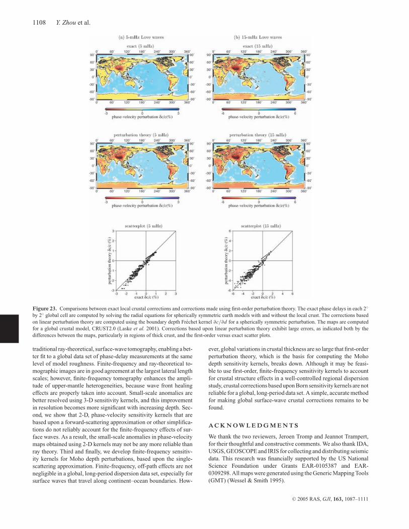
Figure 23. Comparisons between exact local crustal corrections and corrections made using first-order perturbation theory. The exact phase delays in each 2◦by 2◦ global cell are computed by solving the radial equations for spherically symmetric earth models with and without the local crust. The corrections basedon linear perturbation theory are computed using the boundary depth Frechet kernel ∂c/∂d for a spherically symmetric perturbation. The maps are computedfor a global crustal model, CRUST2.0 (Laske et al. 2001). Corrections based upon linear perturbation theory exhibit large errors, as indicated both by thedifferences between the maps, particularly in regions of thick crust, and the first-order versus exact scatter plots.

traditional ray-theoretical, surface-wave tomography, enabling a bet-ter fit to a global data set of phase-delay measurements at the samelevel of model roughness. Finite-frequency and ray-theoretical to-mographic images are in good agreement at the largest lateral lengthscales; however, finite-frequency tomography enhances the ampli-tude of upper-mantle heterogeneities, because wave front healingeffects are properly taken into account. Small-scale anomalies arebetter resolved using 3-D sensitivity kernels, and this improvementin resolution becomes more significant with increasing depth. Sec-ond, we show that 2-D, phase-velocity sensitivity kernels that arebased upon a forward-scattering approximation or other simplifica-tions do not reliably account for the finite-frequency effects of sur-face waves. As a result, the small-scale anomalies in phase-velocitymaps obtained using 2-D kernels may not be any more reliable thanray theory. Third and finally, we develop finite-frequency sensitiv-ity kernels for Moho depth perturbations, based upon the single-scattering approximation. Finite-frequency, off-path effects are notnegligible in a global, long-period dispersion data set, especially forsurface waves that travel along continent–ocean boundaries. How-

ever, global variations in crustal thickness are so large that first-orderperturbation theory, which is the basis for computing the Mohodepth sensitivity kernels, breaks down. Although it may be feasi-ble to use first-order, finite-frequency sensitivity kernels to accountfor crustal structure effects in a well-controlled regional dispersionstudy, crustal corrections based upon Born sensitivity kernels are notreliable for a global, long-period data set. A simple, accurate methodfor making global surface-wave crustal corrections remains to befound.

A C K N O W L E D G M E N T S

We thank the two reviewers, Jeroen Tromp and Jeannot Trampert,for their thoughtful and constructive comments. We also thank IDA,USGS, GEOSCOPE and IRIS for collecting and distributing seismicdata. This research was financially supported by the US NationalScience Foundation under Grants EAR-0105387 and EAR-0309298. All maps were generated using the Generic Mapping Tools(GMT) (Wessel & Smith 1995).

C© 2005 RAS, GJI, 163, 1087–1111

Finite-frequency effects in global surface-wave tomography 1109

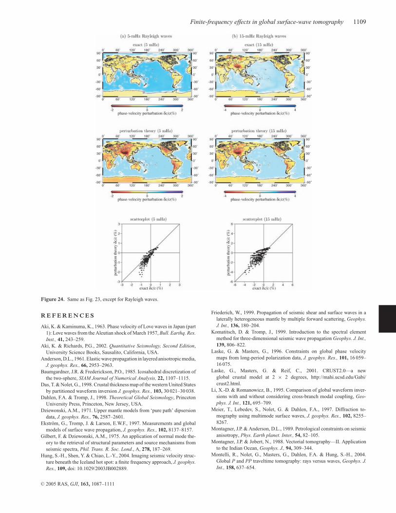
Figure 24. Same as Fig. 23, except for Rayleigh waves.

R E F E R E N C E S

Aki, K. & Kaminuma, K., 1963. Phase velocity of Love waves in Japan (part1): Love waves from the Aleutian shock of March 1957, Bull. Earthq. Res.Inst., 41, 243–259.

Aki, K. & Richards, P.G., 2002. Quantitative Seismology, Second Edition,University Science Books, Sausalito, California, USA.

Anderson, D.L., 1961. Elastic wave propagation in layered anisotropic media,J. geophys. Res., 66, 2953–2963.

Baumgardner, J.R. & Frederickson, P.O., 1985. Icosahedral discretization ofthe two-sphere, SIAM Journal of Numerical Analysis, 22, 1107–1115.

Das, T. & Nolet, G., 1998. Crustal thickness map of the western United Statesby partitioned waveform inversion J. geophys. Res., 103, 30 021–30 038.

Dahlen, F.A. & Tromp, J., 1998. Theoretical Global Seismology, PrincetonUniversity Press, Princeton, New Jersey, USA.

Dziewonski, A.M., 1971. Upper mantle models from ‘pure path’ dipsersiondata, J. geophys. Res., 76, 2587–2601.

Ekstrom, G., Tromp, J. & Larson, E.W.F., 1997. Measurements and globalmodels of surface wave propagation, J. geophys. Res., 102, 8137–8157.

Gilbert, F. & Dziewonski, A.M., 1975. An application of normal mode the-ory to the retrieval of structural parameters and source mechanisms fromseismic spectra, Phil. Trans. R. Soc. Lond., A, 278, 187–269.

Hung, S.-H., Shen, Y. & Chiao, L.-Y., 2004. Imaging seismic velocity struc-ture beneath the Iceland hot spot: a finite frequency approach, J. geophys.Res., 109, doi: 10.1029/2003JB002889.

Friederich, W., 1999. Propagation of seismic shear and surface waves in alaterally heterogeneous mantle by multiple forward scattering, Geophys.J. Int., 136, 180–204.

Komatitsch, D. & Tromp, J., 1999. Introduction to the spectral elementmethod for three-dimensional seismic wave propagation Geophys. J. Int.,139, 806–822.

Laske, G. & Masters, G., 1996. Constraints on global phase velocitymaps from long-period polarization data, J. geophys. Res., 101, 16 059–16 075.

Laske, G., Masters, G. & Reif, C., 2001. CRUST2.0—a newglobal crustal model at 2 × 2 degrees, http://mahi.ucsd.edu/Gabi/crust2.html.

Li, X.-D. & Romanowicz, B., 1995. Comparison of global waveform inver-sions with and without considering cross-branch modal coupling, Geo-phys. J. Int., 121, 695–709.

Meier, T., Lebedev, S., Nolet, G. & Dahlen, F.A., 1997. Diffraction to-mography using multimode surface waves, J. geophys. Res., 102, 8255–8267.

Montagner, J.P. & Anderson, D.L., 1989. Petrological constraints on seismicanisotropy, Phys. Earth planet. Inter., 54, 82–105.

Montagner, J.P. & Jobert, N., 1988. Vectorial tomography—II. Applicationto the Indian Ocean, Geophys. J., 94, 309–344.

Montelli, R., Nolet, G., Masters, G., Dahlen, F.A. & Hung, S.-H., 2004.Global P and PP traveltime tomography: rays versus waves, Geophys. J.Int., 158, 637–654.

C© 2005 RAS, GJI, 163, 1087–1111

1110 Y. Zhou et al.

Paige, C.C. & Saunders, M.A., 1982. LSQR: An algorithm for sparse linearequations and sparse lease squares, ACM TOMS, 8, 43–71.

Ritzwoller, M.H., Shapiro, N.M., Barmin, M.P. & Levshin, A.L., 2002.Global surface wave diffraction tomography, J. geophys. Res., 107, B12,10.1029/2002JB001777.

Spetzler, J., Trampert, J. & Snieder, R., 2002. The effects of scattering insurface wave tomography, Geophys. J. Int., 149, 755–767.

Snieder, R. & Nolet, G., 1987. Linearized scattering of surface waves on aspherical Earth, J. geophys. 61, 55–63.

Trampert, J. & Woodhouse, J.H., 1995. Global phase velocity maps of Loveand Rayleigh waves between 40 and 150 s, Geophys. J. Int., 122, 675–690.

Tromp, J. & Dahlen, F.A., 1992. Variational principles for surface wavepropagation on a laterally heterogeneous Earth—II. Frequency-domainJWKB theory, Geophys. J. Int., 109, 599–619.

Wessel, P. & Smith, W.H.F., 1995. New version of the Generic MappingTools released, EOS, Trans. Am. geophys. Un., 76, 329.

Wielandt, E., 1993. Propagation and structural interpretation of non-planewaves, Geophys. J. Int., 113, 45–53.

Yomogida, K. & Aki, K., 1987. Amplitude and phase data inversions forphase velocity anomalies in the Pacific Ocean basin, Geophys. J. R. astr.Soc., 88, 161–204.

Yoshizawa, K. & Kennett, B.L.N., 2002. Determination of the influence zonefor surface wave paths, Geophys. J. Int., 149, 440–453.

Yoshizawa, K. & Kennett, B.L.N., 2004. Multimode surface wave tomogra-phy for the Australian region using a three-stage approach incorporating fi-nite frequency effects, J. geophys. Res., 109, doi: 10.1029/2002JB002254.

Zhou, Y., Dahlen, F.A. & Nolet, G., 2004. Three-dimensional sensitiv-ity kernels for surface wave observables, Geophys. J. Int., 158, 142–168.

Zhou, Y., Nolet, G., Dahlen, F.A. & Laske, G., 2005. Global upper-mantlestructure from finite-frequency surface-wave tomography, J. geophys.Res., in press.

A P P E N D I X A : B O U N DA RY S C AT T E R I N G C O E F F I C I E N T S

In this appendix, we derive explicit expressions for the boundary scattering coefficients �(1) and �(2) in eqs (6.9), (6.12) and (6.14)–(6.15).The notation used in this appendix is the same as in the appendix of Zhou et al. (2004). The first scattering interaction coefficient �(1) can bewritten as:

�(1) = ρ ω2p′′∗· p′ − λ (tr E′′∗)(tr E′) − µ (E′′∗: E′), (A1)

where p′ = rU′ − i k

′V

′ + i (r × k′)W

′is the polarization vector of surface-wave mode σ ′ along the source-to-scatterer leg, and

p′′ = rU ′′ − i k′′V ′′ + i (r × k′′)W ′′ is the polarization vector of surface-wave mode σ ′′ along the scatterer-to-receiver leg. The quantitiesE ′ = (1/2)[∇p ′ + (∇p ′)T] and E ′′ = (1/2)[∇p′′ + (∇p′′)T] are the associated surface-wave strain tensors, and an asterisk denotes the complexconjugate. All quantities in eq. (A1) are evaluated at the scatterer. The detailed expressions for the scattering coefficient �(1), dependent uponthe scattering interaction, are:Love-to-Love scattering,

�(1)L ′ L ′′ = −ρ ω2W ′′W ′ cos η

+ µ (W ′′ − r−1W ′′)(W ′ − r−1W ′) cos η

+ µ k ′′k ′r−2W ′′W ′ cos 2η;

Rayleigh-to-Rayleigh scattering,

�(1)R′ R′′ = −ρ (U ′′U ′ + V ′′V ′ cos η)

+ λ (U ′ + 2r−1U ′ − k ′r−1V ′)(U ′′ + 2r−1U ′′ − k ′r−1V ′′)

+ µ [ 2U ′′U ′ + r−2(2U ′′ − k ′′V ′′)(2U ′ − k ′V ′) ]

+ µ (V ′′ − r−1V ′′ + k ′′r−1U ′′) (V ′ − r−1V ′ + k ′r−1U ′) cos η

+ µ k ′′k ′r−2V ′′V ′ cos 2η;

Love-to-Rayleigh scattering,

�(1)L ′ R′′ = ρ ω2V ′′W ′ sin η

− µ(V ′′ − r−1V ′′ + k ′′r−1U ′′)(W ′ − r−1W ′) sin η

− µk ′′k ′r−2V ′′W ′ sin 2η;

Rayleigh-to-Love scattering,

�(1)R′ L ′′ = −ρ ω2W ′′V ′ sin η

+ µ(W ′′ − r−1W ′′)(V ′ − r−1V ′ + k ′r−1U ′) sin η

+ µk ′′k ′r−2W ′′V ′ sin 2η.

The second scattering interaction coefficient �(2) can be written as:

σ′ �

(2)σ ′′ = [r · ∇xp′′∗] · {r · [λ(tr E′) I + 2µE′]} + {r · [λ(tr E′′∗)I + 2µE′′∗]} · [r · ∇xp′]. (A2)

In this case the detailed expressions are:Love-to-Love scattering,

�(2)L ′ L ′′ = −µ W ′′ [W ′ − r−1W ′] cos η

−µ W ′ [W ′′ − r−1W ′′] cos η;

C© 2005 RAS, GJI, 163, 1087–1111

Finite-frequency effects in global surface-wave tomography 1111

Rayleigh-to-Rayleigh scattering,

�(2)R′ R′′ = −λ U ′′ [U ′ + 2 r−1U ′ − k ′r−1V ′]

−λ U ′ [U ′′ + 2 r−1U ′′ − k ′′r−1V ′′]

−4µ U ′U ′′

−µ V ′′[V ′ + r−1k ′U ′ − r−1V ′] cos η

−µ V ′ [V ′′ + r−1k ′′U ′′ − r−1V ′′] cos η;

Love-to-Rayleigh scattering,

�(2)L ′ R′′ = µ V ′′ [W ′ − r−1W ′] sin η

+µ W ′ [V ′′ + r−1k ′′U ′′ − r−1V ′′] sin η;

Rayleigh-to-Love scattering,

�(2)R′ L ′′ = −µ V ′ [W ′′ − r−1W ′′] sin η

−µ W ′′ [V ′ + r−1k ′U ′ − r−1V ′] sin η.

The quantity η = arccos(k′ · k′′) is the scattering angle, measured counter-clockwise from the incoming wavevector k

′to the outgoing

wavevector k′′. A dot denotes differentiation of U ′, V ′, W ′ or U ′′, V ′′, W ′′ with respect to radius r.

C© 2005 RAS, GJI, 163, 1087–1111