Study guide: Finite dierence methods for wavemotion

Hans Petter Langtangen1,2

Center for Biomedical Computing, Simula Research Laboratory1

Department of Informatics, University of Oslo2

2016

Finite dierence methods for waves on a string

Waves on a string can be modeled by the wave equation

∂2u

∂t2= c2

∂2u

∂x2

u(x , t) is the displacement of the string

Demo of waves on a string.

The complete initial-boundary value problem

∂2u

∂t2= c2

∂2u

∂x2, x ∈ (0, L), t ∈ (0,T ] (1)

u(x , 0) = I (x), x ∈ [0, L] (2)

∂

∂tu(x , 0) = 0, x ∈ [0, L] (3)

u(0, t) = 0, t ∈ (0,T ] (4)

u(L, t) = 0, t ∈ (0,T ] (5)

Input data in the problem

Initial condition u(x , 0) = I (x): initial string shape

Initial condition ut(x , 0) = 0: string starts from rest

c =√

T/%: velocity of waves on the string

(T is the tension in the string, % is density of the string)

Two boundary conditions on u: u = 0 means xed ends (nodisplacement)

Rule for number of initial and boundary conditions:

utt in the PDE: two initial conditions, on u and ut

ut (and no utt) in the PDE: one initial conditions, on u

uxx in the PDE: one boundary condition on u at eachboundary point

Demo of a vibrating string (C = 0.8)

Our numerical method is sometimes exact (!)

Our numerical method is sometimes subject to seriousnon-physical eects

Demo of a vibrating string (C = 1.0012)

Ooops!

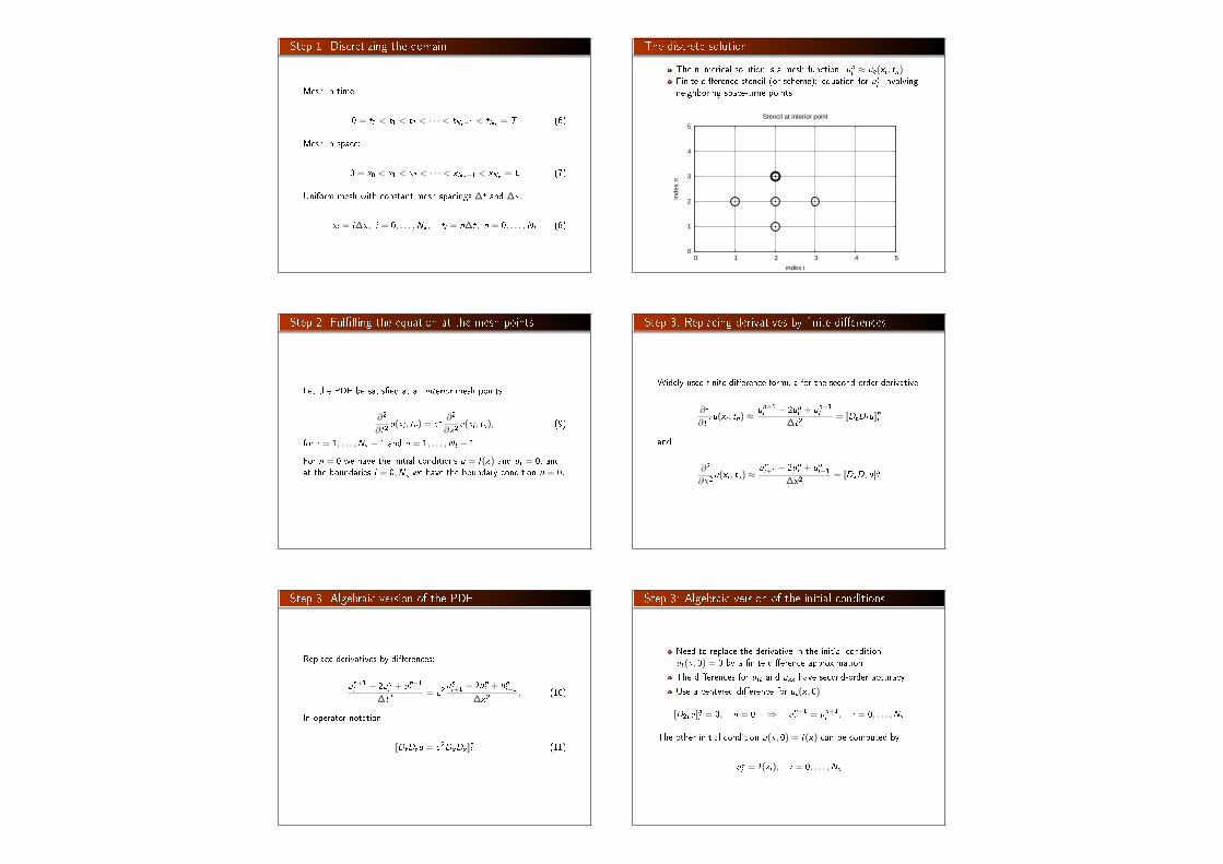
Step 1: Discretizing the domain

Mesh in time:

0 = t0 < t1 < t2 < · · · < tNt−1 < tNt= T (6)

Mesh in space:

0 = x0 < x1 < x2 < · · · < xNx−1 < xNx= L (7)

Uniform mesh with constant mesh spacings ∆t and ∆x :

xi = i∆x , i = 0, . . . ,Nx , ti = n∆t, n = 0, . . . ,Nt (8)

The discrete solution

The numerical solution is a mesh function: uni ≈ ue(xi , tn)Finite dierence stencil (or scheme): equation for uni involvingneighboring space-time points

0

1

2

3

4

5

0 1 2 3 4 5

inde

x n

index i

Stencil at interior point

Step 2: Fullling the equation at the mesh points

Let the PDE be satised at all interior mesh points:

∂2

∂t2u(xi , tn) = c2

∂2

∂x2u(xi , tn), (9)

for i = 1, . . . ,Nx − 1 and n = 1, . . . ,Nt − 1.

For n = 0 we have the initial conditions u = I (x) and ut = 0, andat the boundaries i = 0,Nx we have the boundary condition u = 0.

Step 3: Replacing derivatives by nite dierences

Widely used nite dierence formula for the second-order derivative:

∂2

∂t2u(xi , tn) ≈ un+1

i − 2uni + un−1i

∆t2= [DtDtu]ni

and

∂2

∂x2u(xi , tn) ≈ uni+1 − 2uni + uni−1

∆x2= [DxDxu]ni

Step 3: Algebraic version of the PDE

Replace derivatives by dierences:

un+1i − 2uni + un−1i

∆t2= c2

uni+1 − 2uni + uni−1∆x2

, (10)

In operator notation:

[DtDtu = c2DxDx ]ni (11)

Step 3: Algebraic version of the initial conditions

Need to replace the derivative in the initial conditionut(x , 0) = 0 by a nite dierence approximation

The dierences for utt and uxx have second-order accuracy

Use a centered dierence for ut(x , 0)

[D2tu]ni = 0, n = 0 ⇒ un−1i = un+1i , i = 0, . . . ,Nx

The other initial condition u(x , 0) = I (x) can be computed by

u0i = I (xi ), i = 0, . . . ,Nx

Step 4: Formulating a recursive algorithm

Nature of the algorithm: compute u in space att = ∆t, 2∆t, 3∆t, ...

Three time levels are involved in the general discrete equation:n + 1, n, n − 1

uni and un−1i are then already computed for i = 0, . . . ,Nx , andun+1i is the unknown quantity

Write out [DtDtu = c2DxDx ]ni and solve for un+1i ,

un+1i = −un−1i + 2uni + C 2

(uni+1 − 2uni + uni−1

)(12)

The Courant number

C = c∆t

∆x, (13)

is known as the (dimensionless) Courant number

Observe

There is only one parameter, C , in the discrete model: C lumpsmesh parameters ∆t and ∆x with the only physical parameter, thewave velocity c . The value C and the smoothness of I (x) governthe quality of the numerical solution.

The nite dierence stencil

0

1

2

3

4

5

0 1 2 3 4 5

inde

x n

index i

Stencil at interior point

The stencil for the rst time level

Problem: the stencil for n = 1 involves u−1i , but timet = −∆t is outside the mesh

Remedy: use the initial condition ut = 0 together with thestencil to eliminate u−1i

Initial condition:

[D2tu = 0]0i ⇒ u−1i = u1i

Insert in stencil [DtDtu = c2DxDx ]0i to get

u1i = u0i +1

2C 2(uni+1 − 2uni + uni−1

)(14)

The algorithm

1 Compute u0i = I (xi ) for i = 0, . . . ,Nx

2 Compute u1i by (14) and set u1i = 0 for the boundary pointsi = 0 and i = Nx , for n = 1, 2, . . . ,N − 1,

3 For each time level n = 1, 2, . . . ,Nt − 11 apply (12) to nd un+1

i for i = 1, . . . ,Nx − 12 set un+1

i = 0 for the boundary points i = 0, i = Nx .

Moving nite dierence stencil

web page or a movie le.

Sketch of an implementation (1)

Arrays:

u[i] stores un+1

i

u_1[i] stores uni

u_2[i] stores un−1

i

Naming convention

u is the unknown to be computed (a spatial mesh function), u_1denotes the latest computed time level, u_2 corresponds to onetime step back in time.

PDE solvers should save memory

Important to minimize the memory usage

The algorithm only needs to access the three most recent timelevels, so we need only three arrays for un+1

i , uni , and un−1i ,i = 0, . . . ,Nx . Storing all the solutions in a two-dimensional arrayof size (Nx + 1)× (Nt + 1) would be possible in this simpleone-dimensional PDE problem, but not in large 2D problems andnot even in small 3D problems.

Sketch of an implementation (2)

# Given mesh points as arrays x and t (x[i], t[n])dx = x[1] - x[0]dt = t[1] - t[0]C = c*dt/dx # Courant numberNt = len(t)-1C2 = C**2 # Help variable in the scheme

# Set initial condition u(x,0) = I(x)for i in range(0, Nx+1):

u_1[i] = I(x[i])

# Apply special formula for first step, incorporating du/dt=0for i in range(1, Nx):

u[i] = u_1[i] + 0.5*C**2(u_1[i+1] - 2*u_1[i] + u_1[i-1])u[0] = 0; u[Nx] = 0 # Enforce boundary conditions

# Switch variables before next stepu_2[:], u_1[:] = u_1, u

for n in range(1, Nt):# Update all inner mesh points at time t[n+1]for i in range(1, Nx):

u[i] = 2*u_1[i] - u_2[i] + \C**2(u_1[i+1] - 2*u_1[i] + u_1[i-1])

# Insert boundary conditionsu[0] = 0; u[Nx] = 0

# Switch variables before next stepu_2[:], u_1[:] = u_1, u

Verication

Think about testing and verication before you startimplementing the algorithm!

Powerful testing tool: method of manufactured solutions andcomputation of convergence rates

Will need a source term in the PDE and ut(x , 0) 6= 0

Even more powerful method: exact solution of the scheme

A slightly generalized model problem

Add source term f and nonzero initial condition ut(x , 0):

utt = c2uxx + f (x , t), (15)

u(x , 0) = I (x), x ∈ [0, L] (16)

ut(x , 0) = V (x), x ∈ [0, L] (17)

u(0, t) = 0, t > 0, (18)

u(L, t) = 0, t > 0 (19)

Discrete model for the generalized model problem

[DtDtu = c2DxDx + f ]ni (20)

Writing out and solving for the unknown un+1i :

un+1i = −un−1i + 2uni + C 2(uni+1 − 2uni + uni−1) + ∆t2f ni (21)

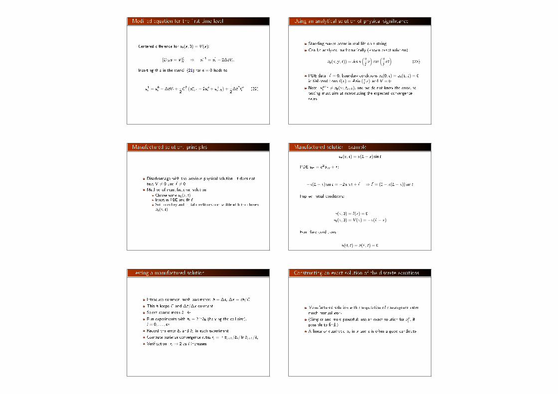
Modied equation for the rst time level

Centered dierence for ut(x , 0) = V (x):

[D2tu = V ]0i ⇒ u−1i = u1i − 2∆tVi ,

Inserting this in the stencil (21) for n = 0 leads to

u1i = u0i −∆tVi +1

2C 2(uni+1 − 2uni + uni−1

)+

1

2∆t2f ni (22)

Using an analytical solution of physical signicance

Standing waves occur in real life on a string

Can be analyzed mathematically (known exact solution)

ue(x , y , t)) = A sin(πLx)cos(πLct)

(23)

PDE data: f = 0, boundary conditions ue(0, t) = ue(L, t) = 0,initial conditions I (x) = A sin

(πLx)and V = 0

Note: un+1i 6= ue(xi , tn+1), and we do not know the error, so

testing must aim at reproducing the expected convergencerates

Manufactured solution: principles

Disadvantage with the previous physical solution: it does nottest V 6= 0 and f 6= 0

Method of manufactured solution:

Choose some ue(x , t)Insert in PDE and t f

Set boundary and initial conditions compatible with the chosenue(x , t)

Manufactured solution: example

ue(x , t) = x(L− x) sin t

PDE utt = c2uxx + f :

−x(L− x) sin t = −2 sin t + f ⇒ f = (2− x(L− x)) sin t

Implied initial conditions:

u(x , 0) = I (x) = 0

ut(x , 0) = V (x) = −x(L− x)

Boundary conditions:

u(0, t) = u(L, t) = 0

Testing a manufactured solution

Introduce common mesh parameter: h = ∆t, ∆x = ch/C

This h keeps C and ∆t/∆x constant

Select coarse mesh h: h0

Run experiments with hi = 2−ih0 (halving the cell size),i = 0, . . . ,m

Record the error Ei and hi in each experiment

Compute pariwise convergence rates ri = lnEi+1/Ei/ ln hi+1/hi

Verication: ri → 2 as i increases

Constructing an exact solution of the discrete equations

Manufactured solution with computation of convergence rates:much manual work

(Simpler and more powerful: use an exact solution for uni , ifpossible to nd.)

A linear or quadratic ue in x and t is often a good candidate

Analytical work with the PDE problem

Here, choose ue such that ue(0, t) = ue(L, t) = 0:

ue(x , t) = x(L− x)(1 +1

2t),

Insert in the PDE and nd f :

f (x , t) = 2(1 + t)c2

Initial conditions:

I (x) = x(L− x), V (x) =1

2x(L− x)

Analytical work with the discrete equations (1)

We want to show that ue also solves the discrete equations!

Useful preliminary result:

[DtDtt2]n =

t2n+1 − 2t2n + t2n−1∆t2

= (n + 1)2 − n2 + (n − 1)2 = 2

(24)

[DtDtt]n =tn+1 − 2tn + tn−1

∆t2=

((n + 1)− n + (n − 1))∆t

∆t2= 0

(25)

Hence,

[DtDtue]ni = xi (L− xi )[DtDt(1 +1

2t)]n = xi (L− xi )

1

2[DtDtt]n = 0

Analytical work with the discrete equations (1)

[DxDxue]ni = (1 +1

2tn)[DxDx(xL− x2)]i = (1 +

1

2tn)[LDxDxx − DxDxx

2]i

= −2(1 +1

2tn)

Now, f ni = 2(1 + 12 tn)c2 and we get

[DtDtue−c2DxDxue−f ]ni = 0−c2(−1)2(1+1

2tn)+2(1+

1

2tn)c2 = 0

Moreover, ue(xi , 0) = I (xi ), ∂ue/∂t = V (xi ) at t = 0, andue(x0, t) = ue(xNx

, t) = 0. Also the modied scheme for the rsttime step is fullled by ue(xi , tn).

Testing with the exact discrete solution

We have established thatun+1i = ue(xi , tn+1) = xi (L− xi )(1 + tn+1/2)

Run one simulation with one choice of c , ∆t, and ∆x

Check that maxi |un+1i − ue(xi , tn+1)| < ε, ε ∼ 10−14 (machine

precision + some round-o errors)

This is the simplest and best verication test

Later we show that the exact solution of the discrete equations canbe obtained by C = 1 (!)

Implementation The algorithm

1 Compute u0i = I (xi ) for i = 0, . . . ,Nx

2 Compute u1i by (14) and set u1i = 0 for the boundary pointsi = 0 and i = Nx , for n = 1, 2, . . . ,N − 1,

3 For each time level n = 1, 2, . . . ,Nt − 11 apply (12) to nd un+1

i for i = 1, . . . ,Nx − 12 set un+1

i = 0 for the boundary points i = 0, i = Nx .

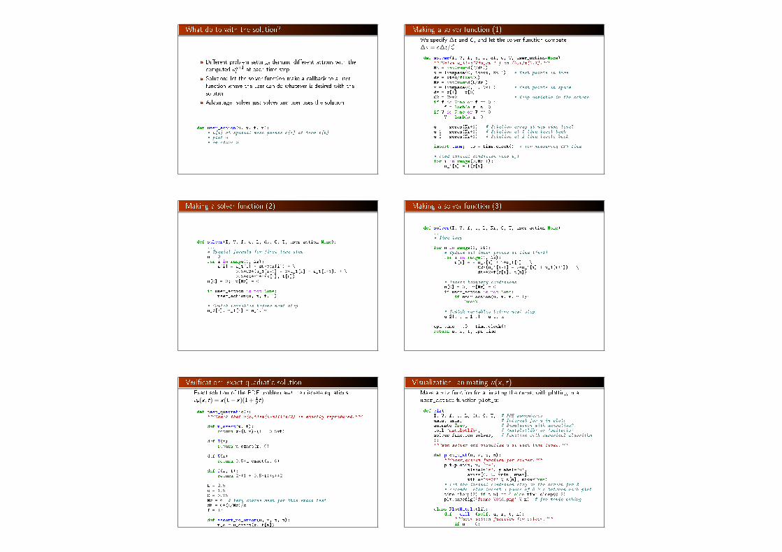
What do to with the solution?

Dierent problem settings demand dierent actions with thecomputed un+1

i at each time step

Solution: let the solver function make a callback to a userfunction where the user can do whatever is desired with thesolution

Advantage: solver just solves and user uses the solution

def user_action(u, x, t, n):# u[i] at spatial mesh points x[i] at time t[n]# plot u# or store u

Making a solver function (1)We specify ∆t and C , and let the solver function compute∆x = c∆t/C .

def solver(I, V, f, c, L, dt, C, T, user_action=None):"""Solve u_tt=c^2*u_xx + f on (0,L)x(0,T]."""Nt = int(round(T/dt))t = linspace(0, Nt*dt, Nt+1) # Mesh points in timedx = dt*c/float(C)Nx = int(round(L/dx))x = linspace(0, L, Nx+1) # Mesh points in spacedx = x[1] - x[0]C2 = C**2 # Help variable in the schemeif f is None or f == 0 :

f = lambda x, t: 0if V is None or V == 0:

V = lambda x: 0

u = zeros(Nx+1) # Solution array at new time levelu_1 = zeros(Nx+1) # Solution at 1 time level backu_2 = zeros(Nx+1) # Solution at 2 time levels back

import time; t0 = time.clock() # for measuring CPU time

# Load initial condition into u_1for i in range(0,Nx+1):

u_1[i] = I(x[i])

if user_action is not None:user_action(u_1, x, t, 0)

Making a solver function (2)

def solver(I, V, f, c, L, dt, C, T, user_action=None):...# Special formula for first time stepn = 0for i in range(1, Nx):

u[i] = u_1[i] + dt*V(x[i]) + \0.5*C2*(u_1[i-1] - 2*u_1[i] + u_1[i+1]) + \0.5*dt**2*f(x[i], t[n])

u[0] = 0; u[Nx] = 0

if user_action is not None:user_action(u, x, t, 1)

# Switch variables before next stepu_2[:], u_1[:] = u_1, u

Making a solver function (3)

def solver(I, V, f, c, L, Nx, C, T, user_action=None):...# Time loop

for n in range(1, Nt):# Update all inner points at time t[n+1]for i in range(1, Nx):

u[i] = - u_2[i] + 2*u_1[i] + \C2*(u_1[i-1] - 2*u_1[i] + u_1[i+1]) + \dt**2*f(x[i], t[n])

# Insert boundary conditionsu[0] = 0; u[Nx] = 0if user_action is not None:

if user_action(u, x, t, n+1):break

# Switch variables before next stepu_2[:], u_1[:] = u_1, u

cpu_time = t0 - time.clock()return u, x, t, cpu_time

Verication: exact quadratic solutionExact solution of the PDE problem and the discrete equations:ue(x , t) = x(L− x)(1 + 1

2 t)

def test_quadratic():"""Check that u(x,t)=x(L-x)(1+t/2) is exactly reproduced."""

def u_exact(x, t):return x*(L-x)*(1 + 0.5*t)

def I(x):return u_exact(x, 0)

def V(x):return 0.5*u_exact(x, 0)

def f(x, t):return 2*(1 + 0.5*t)*c**2

L = 2.5c = 1.5C = 0.75Nx = 6 # Very coarse mesh for this exact testdt = C*(L/Nx)/cT = 18

def assert_no_error(u, x, t, n):u_e = u_exact(x, t[n])diff = np.abs(u - u_e).max()tol = 1E-13assert diff < tol

solver(I, V, f, c, L, dt, C, T,user_action=assert_no_error)

Visualization: animating u(x , t)Make a viz function for animating the curve, with plotting in auser_action function plot_u:

def viz(I, V, f, c, L, dt, C, T, # PDE paramteresumin, umax, # Interval for u in plotsanimate=True, # Simulation with animation?tool='matplotlib', # 'matplotlib' or 'scitools'solver_function=solver, # Function with numerical algorithm):"""Run solver and visualize u at each time level."""

def plot_u_st(u, x, t, n):"""user_action function for solver."""plt.plot(x, u, 'r-',

xlabel='x', ylabel='u',axis=[0, L, umin, umax],title='t=%f' % t[n], show=True)

# Let the initial condition stay on the screen for 2# seconds, else insert a pause of 0.2 s between each plottime.sleep(2) if t[n] == 0 else time.sleep(0.2)plt.savefig('frame_%04d.png' % n) # for movie making

class PlotMatplotlib:def __call__(self, u, x, t, n):

"""user_action function for solver."""if n == 0:

plt.ion()self.lines = plt.plot(x, u, 'r-')plt.xlabel('x'); plt.ylabel('u')plt.axis([0, L, umin, umax])plt.legend(['t=%f' % t[n]], loc='lower left')

else:self.lines[0].set_ydata(u)plt.legend(['t=%f' % t[n]], loc='lower left')plt.draw()

time.sleep(2) if t[n] == 0 else time.sleep(0.2)plt.savefig('tmp_%04d.png' % n) # for movie making

if tool == 'matplotlib':import matplotlib.pyplot as pltplot_u = PlotMatplotlib()

elif tool == 'scitools':import scitools.std as plt # scitools.easyviz interfaceplot_u = plot_u_st

import time, glob, os

# Clean up old movie framesfor filename in glob.glob('tmp_*.png'):

os.remove(filename)

# Call solver and do the simulatonuser_action = plot_u if animate else Noneu, x, t, cpu = solver_function(

I, V, f, c, L, dt, C, T, user_action)

# Make video filesfps = 4 # frames per secondcodec2ext = dict(flv='flv', libx264='mp4', libvpx='webm',

libtheora='ogg') # video formatsfilespec = 'tmp_%04d.png'movie_program = 'ffmpeg' # or 'avconv'for codec in codec2ext:

ext = codec2ext[codec]cmd = '%(movie_program)s -r %(fps)d -i %(filespec)s '\

'-vcodec %(codec)s movie.%(ext)s' % vars()os.system(cmd)

if tool == 'scitools':# Make an HTML play for showing the animation in a browserplt.movie('tmp_*.png', encoder='html', fps=fps,

output_file='movie.html')return cpu

Note: plot_u is function inside function and remembers the localvariables in viz (known as a closure).

Making movie les

Store spatial curve in a le, for each time level

Name les like 'something_%04d.png' % frame_counter

Combine les to a movie

Terminal> scitools movie encoder=html output_file=movie.html \fps=4 frame_*.png # web page with a player

Terminal> avconv -r 4 -i frame_%04d.png -c:v flv movie.flvTerminal> avconv -r 4 -i frame_%04d.png -c:v libtheora movie.oggTerminal> avconv -r 4 -i frame_%04d.png -c:v libx264 movie.mp4Terminal> avconv -r 4 -i frame_%04d.png -c:v libpvx movie.webm

Important

Zero padding (%04d) is essential for correct sequence of framesin something_*.png (Unix alphanumeric sort)

Remove old frame_*.png les before making a new movie

Running a case

Vibrations of a guitar string

Triangular initial shape (at rest)

I (x) =

ax/x0, x < x0a(L− x)/(L− x0), otherwise

(26)

Appropriate data:

L = 75 cm, x0 = 0.8L, a = 5 mm, time frequency ν = 440 Hz

Implementation of the case

def guitar(C):"""Triangular wave (pulled guitar string)."""L = 0.75x0 = 0.8*La = 0.005freq = 440wavelength = 2*Lc = freq*wavelengthomega = 2*pi*freqnum_periods = 1T = 2*pi/omega*num_periods# Choose dt the same as the stability limit for Nx=50dt = L/50./c

def I(x):return a*x/x0 if x < x0 else a/(L-x0)*(L-x)

umin = -1.2*a; umax = -umincpu = viz(I, 0, 0, c, L, dt, C, T, umin, umax,

animate=True, tool='scitools')

Program: wave1D_u0.py.

Resulting movie for C = 0.8

Movie of the vibrating string

The benets of scaling

It is dicult to gure out all the physical parameters of a case

And it is not necessary because of a powerful: scaling

Introduce new x , t, and u without dimension:

x =x

L, t =

c

Lt, u =

u

a

Insert this in the PDE (with f = 0) and dropping bars

utt = uxx

Initial condition: set a = 1, L = 1, and x0 ∈ [0, 1] in (26).

In the code: set a=c=L=1, x0=0.8, and there is no need tocalculate with wavelengths and frequencies to estimate c!

Just one challenge: determine the period of the waves and anappropriate end time (see the text for details).

Vectorization

Problem: Python loops over long arrays are slow

One remedy: use vectorized (numpy) code instead of explicitloops

Other remedies: use Cython, port spatial loops to Fortran or C

Speedup: 100-1000 (varies with Nx)

Next: vectorized loops

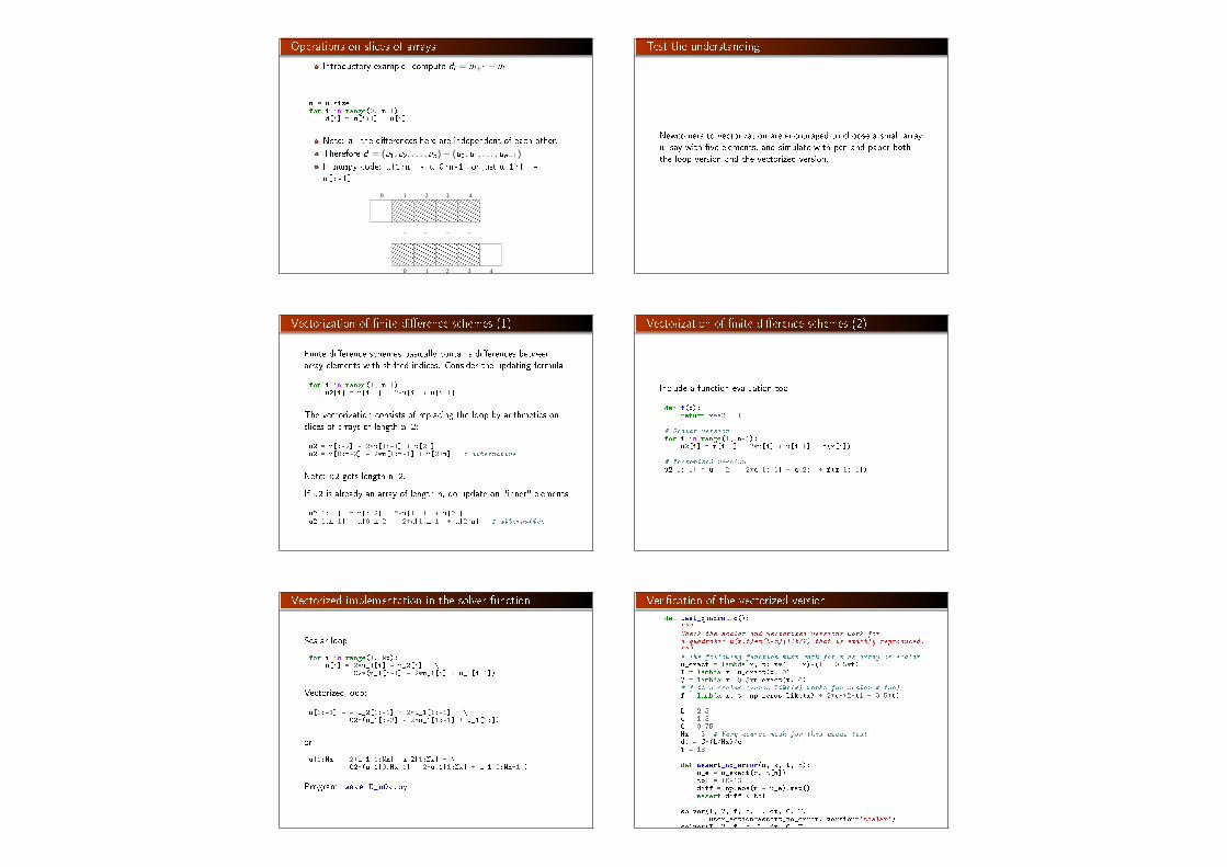
Operations on slices of arrays

Introductory example: compute di = ui+1 − ui

n = u.sizefor i in range(0, n-1):

d[i] = u[i+1] - u[i]

Note: all the dierences here are independent of each other.

Therefore d = (u1, u2, . . . , un)− (u0, u1, . . . , un−1)

In numpy code: u[1:n] - u[0:n-1] or just u[1:] -

u[:-1]

− −−−

0 1 2 3 4

0 1 2 3 4

Test the understanding

Newcomers to vectorization are encouraged to choose a small arrayu, say with ve elements, and simulate with pen and paper boththe loop version and the vectorized version.

Vectorization of nite dierence schemes (1)

Finite dierence schemes basically contains dierences betweenarray elements with shifted indices. Consider the updating formula

for i in range(1, n-1):u2[i] = u[i-1] - 2*u[i] + u[i+1]

The vectorization consists of replacing the loop by arithmetics onslices of arrays of length n-2:

u2 = u[:-2] - 2*u[1:-1] + u[2:]u2 = u[0:n-2] - 2*u[1:n-1] + u[2:n] # alternative

Note: u2 gets length n-2.

If u2 is already an array of length n, do update on "inner" elements

u2[1:-1] = u[:-2] - 2*u[1:-1] + u[2:]u2[1:n-1] = u[0:n-2] - 2*u[1:n-1] + u[2:n] # alternative

Vectorization of nite dierence schemes (2)

Include a function evaluation too:

def f(x):return x**2 + 1

# Scalar versionfor i in range(1, n-1):

u2[i] = u[i-1] - 2*u[i] + u[i+1] + f(x[i])

# Vectorized versionu2[1:-1] = u[:-2] - 2*u[1:-1] + u[2:] + f(x[1:-1])

Vectorized implementation in the solver function

Scalar loop:

for i in range(1, Nx):u[i] = 2*u_1[i] - u_2[i] + \

C2*(u_1[i-1] - 2*u_1[i] + u_1[i+1])

Vectorized loop:

u[1:-1] = - u_2[1:-1] + 2*u_1[1:-1] + \C2*(u_1[:-2] - 2*u_1[1:-1] + u_1[2:])

or

u[1:Nx] = 2*u_1[1:Nx]- u_2[1:Nx] + \C2*(u_1[0:Nx-1] - 2*u_1[1:Nx] + u_1[2:Nx+1])

Program: wave1D_u0v.py

Verication of the vectorized version

def test_quadratic():"""Check the scalar and vectorized versions work fora quadratic u(x,t)=x(L-x)(1+t/2) that is exactly reproduced."""# The following function must work for x as array or scalaru_exact = lambda x, t: x*(L - x)*(1 + 0.5*t)I = lambda x: u_exact(x, 0)V = lambda x: 0.5*u_exact(x, 0)# f is a scalar (zeros_like(x) works for scalar x too)f = lambda x, t: np.zeros_like(x) + 2*c**2*(1 + 0.5*t)

L = 2.5c = 1.5C = 0.75Nx = 3 # Very coarse mesh for this exact testdt = C*(L/Nx)/cT = 18

def assert_no_error(u, x, t, n):u_e = u_exact(x, t[n])tol = 1E-13diff = np.abs(u - u_e).max()assert diff < tol

solver(I, V, f, c, L, dt, C, T,user_action=assert_no_error, version='scalar')

solver(I, V, f, c, L, dt, C, T,user_action=assert_no_error, version='vectorized')

Note:

Compact code with lambda functionsThe scalar f value needs careful coding: return constant arrayif vectorized code, else number

Eciency measurements

Run wave1D_u0v.py for Nx as 50,100,200,400,800 andmeasuring the CPU time

Observe substantial speed-up: vectorized version is aboutNx/5 times faster

Much bigger improvements for 2D and 3D codes!

Generalization: reecting boundaries

Boundary condition u = 0: u changes sign

Boundary condition ux = 0: wave is perfectly reected

How can we implement ux? (more complicated than u = 0)

Demo of boundary conditions

Neumann boundary condition

∂u

∂n≡ n · ∇u = 0 (27)

For a 1D domain [0, L]:

∂

∂n

∣∣∣∣x=L

=∂

∂x,

∂

∂n

∣∣∣∣x=0

= − ∂

∂x

Boundary condition terminology:

ux specied: Neumann condition

u specied: Dirichlet condition

Discretization of derivatives at the boundary (1)

How can we incorporate the condition ux = 0 in the nitedierence scheme?

We used centeral dierences for utt and uxx : O(∆t2,∆x2)accuracy

Also for ut(x , 0)

Should use central dierence for ux to preserve second orderaccuracy

un−1 − un12∆x

= 0 (28)

Discretization of derivatives at the boundary (2)

un−1 − un12∆x

= 0

Problem: un−1 is outside the mesh (ctitious value)

Remedy: use the stencil at the boundary to eliminate un−1; justreplace un−1 by un1

un+1i = −un−1i + 2uni + 2C 2

(uni+1 − uni

), i = 0 (29)

Visualization of modied boundary stencil

Discrete equation for computing u30 in terms of u20 , u10 , and u21 :

Animation in a web page or a movie le.

Implementation of Neumann conditions

Use the general stencil for interior points also on the boundary

Replace uni−1 by uni+1 for i = 0

Replace uni+1 by uni−1 for i = Nx

i = 0ip1 = i+1im1 = ip1 # i-1 -> i+1u[i] = u_1[i] + C2*(u_1[im1] - 2*u_1[i] + u_1[ip1])

i = Nxim1 = i-1ip1 = im1 # i+1 -> i-1u[i] = u_1[i] + C2*(u_1[im1] - 2*u_1[i] + u_1[ip1])

# Or just one loop over all points

for i in range(0, Nx+1):ip1 = i+1 if i < Nx else i-1im1 = i-1 if i > 0 else i+1u[i] = u_1[i] + C2*(u_1[im1] - 2*u_1[i] + u_1[ip1])

Program wave1D_dn0.py

Moving nite dierence stencil

web page or a movie le.

Index set notation

Tedious to write index sets like i = 0, . . . ,Nx andn = 0, . . . ,Nt

Notation not valid if i or n starts at 1 instead...

Both in math and code it is advantageous to use index sets

i ∈ Ix instead of i = 0, . . . ,Nx

Denition: Ix = 0, . . . ,NxThe rst index: i = I0xThe last index: i = I−1x

All interior points: i ∈ I ix , I ix = 1, . . . ,Nx − 1I−x means 0, . . . ,Nx − 1I+x means 1, . . . ,Nx

Index set notation in code

Notation Python

Ix Ix

I0

x Ix[0]

I−1

x Ix[-1]

I+x Ix[1:]

I−x Ix[:-1]

I ix Ix[1:-1]

Index sets in action (1)

Index sets for a problem in the x , t plane:

Ix = 0, . . . ,Nx, It = 0, . . . ,Nt, (30)

Implemented in Python as

Ix = range(0, Nx+1)It = range(0, Nt+1)

Index sets in action (2)

A nite dierence scheme can with the index set notation bespecied as

un+1i = −un−1i + 2uni + C 2

(uni+1 − 2uni + uni−1

), i ∈ I ix , n ∈ I it

un+1i = 0, i = I0x , n ∈ I it

un+1i = 0, i = I−1x , n ∈ I it

Corresponding implementation:

for n in It[1:-1]:for i in Ix[1:-1]:

u[i] = - u_2[i] + 2*u_1[i] + \C2*(u_1[i-1] - 2*u_1[i] + u_1[i+1])

i = Ix[0]; u[i] = 0i = Ix[-1]; u[i] = 0

Program wave1D_dn.py

Alternative implementation via ghost cells

Instead of modifying the stencil at the boundary, we extendthe mesh to cover un−1 and unNx+1

The extra left and right cell are called ghost cells

The extra points are called ghost points

The un−1 and unNx+1 values are called ghost values

Update ghost values as uni−1 = uni+1 for i = 0 and uni+1 = uni−1for i = Nx

Then the stencil becomes right at the boundary

Implementation of ghost cells (1)

Add ghost points:

u = zeros(Nx+3)u_1 = zeros(Nx+3)u_2 = zeros(Nx+3)

x = linspace(0, L, Nx+1) # Mesh points without ghost points

A major indexing problem arises with ghost cells since Pythonindices must start at 0.

u[-1] will always mean the last element in u

Math indexing: −1, 0, 1, 2, . . . ,Nx + 1

Python indexing: 0,..,Nx+2

Remedy: use index sets

Implementation of ghost cells (2)

u = zeros(Nx+3)Ix = range(1, u.shape[0]-1)

# Boundary values: u[Ix[0]], u[Ix[-1]]

# Set initial conditionsfor i in Ix:

u_1[i] = I(x[i-Ix[0]]) # Note i-Ix[0]

# Loop over all physical mesh pointsfor i in Ix:

u[i] = - u_2[i] + 2*u_1[i] + \C2*(u_1[i-1] - 2*u_1[i] + u_1[i+1])

# Update ghost valuesi = Ix[0] # x=0 boundaryu[i-1] = u[i+1]i = Ix[-1] # x=L boundaryu[i+1] = u[i-1]

Program: wave1D_dn0_ghost.py.

Generalization: variable wave velocity

Heterogeneous media: varying c = c(x)

The model PDE with a variable coecient

∂2u

∂t2=

∂

∂x

(q(x)

∂u

∂x

)+ f (x , t) (31)

This equation sampled at a mesh point (xi , tn):

∂2

∂t2u(xi , tn) =

∂

∂x

(q(xi )

∂

∂xu(xi , tn)

)+ f (xi , tn),

Discretizing the variable coecient (1)

The principal idea is to rst discretize the outer derivative.

Dene

φ = q(x)∂u

∂x

Then use a centered derivative around x = xi for the derivative ofφ:

[∂φ

∂x

]n

i

≈φi+ 1

2

− φi− 1

2

∆x= [Dxφ]ni

Discretizing the variable coecient (2)

Then discretize the inner operators:

φi+ 1

2

= qi+ 1

2

[∂u

∂x

]n

i+ 1

2

≈ qi+ 1

2

uni+1 − uni∆x

= [qDxu]ni+ 1

2

Similarly,

φi− 1

2

= qi− 1

2

[∂u

∂x

]n

i− 1

2

≈ qi− 1

2

uni − uni−1∆x

= [qDxu]ni− 1

2

Discretizing the variable coecient (3)

These intermediate results are now combined to

[∂

∂x

(q(x)

∂u

∂x

)]n

i

≈ 1

∆x2

(qi+ 1

2

(uni+1 − uni

)− qi− 1

2

(uni − uni−1

))

(32)

In operator notation:

[∂

∂x

(q(x)

∂u

∂x

)]n

i

≈ [DxqDxu]ni (33)

Remark

Many are tempted to use the chain rule on the term ∂∂x

(q(x)∂u∂x

),

but this is not a good idea!

Computing the coecient between mesh points

Given q(x): compute qi+ 1

2

as q(xi+ 1

2

)

Given q at the mesh points: qi , use an average

qi+ 1

2

≈ 1

2(qi + qi+1) = [qx ]i (arithmetic mean) (34)

qi+ 1

2

≈ 2

(1

qi+

1

qi+1

)−1(harmonic mean) (35)

qi+ 1

2

≈ (qiqi+1)1/2 (geometric mean) (36)

The arithmetic mean in (34) is by far the most used averagingtechnique.

Discretization of variable-coecient wave equation inoperator notation

[DtDtu = DxqxDxu + f ]ni (37)

We clearly see the type of nite dierences and averaging!

Write out and solve wrt un+1i :

un+1i = −un−1i + 2uni +

(∆t

∆x

)2

×(1

2(qi + qi+1)(uni+1 − uni )− 1

2(qi + qi−1)(uni − uni−1)

)+

∆t2f ni (38)

Neumann condition and a variable coecient

Consider ∂u/∂x = 0 at x = L = Nx∆x :

uni+1 − uni−12∆x

= 0 uni+1 = uni−1, i = Nx

Insert uni+1 = uni−1 in the stencil (38) for i = Nx and obtain

un+1i ≈ −un−1i + 2uni +

(∆t

∆x

)2

2qi (uni−1 − uni ) + ∆t2f ni

(We have used qi+ 1

2

+ qi− 1

2

≈ 2qi .)

Alternative: assume dq/dx = 0 (simpler).

Implementation of variable coecients

Assume c[i] holds ci the spatial mesh points

for i in range(1, Nx):u[i] = - u_2[i] + 2*u_1[i] + \

C2*(0.5*(q[i] + q[i+1])*(u_1[i+1] - u_1[i]) - \0.5*(q[i] + q[i-1])*(u_1[i] - u_1[i-1])) + \

dt2*f(x[i], t[n])

Here: C2=(dt/dx)**2

Vectorized version:

u[1:-1] = - u_2[1:-1] + 2*u_1[1:-1] + \C2*(0.5*(q[1:-1] + q[2:])*(u_1[2:] - u_1[1:-1]) -

0.5*(q[1:-1] + q[:-2])*(u_1[1:-1] - u_1[:-2])) + \dt2*f(x[1:-1], t[n])

Neumann condition ux = 0: same ideas as in 1D (modied stencilor ghost cells).

A more general model PDE with variable coecients

%(x)∂2u

∂t2=

∂

∂x

(q(x)

∂u

∂x

)+ f (x , t) (39)

A natural scheme is

[%DtDtu = DxqxDxu + f ]ni (40)

Or

[DtDtu = %−1DxqxDxu + f ]ni (41)

No need to average %, just sample at i

Generalization: dampingWhy do waves die out?

Damping (non-elastic eects, air resistance)2D/3D: conservation of energy makes an amplitude reductionby 1/

√r (2D) or 1/r (3D)

Simplest damping model (for physical behavior, see demo):

∂2u

∂t2+ b

∂u

∂t= c2

∂2u

∂x2+ f (x , t), (42)

b ≥ 0: prescribed damping coecient.

Discretization via centered dierences to ensure O(∆t2) error:

[DtDtu + bD2tu = c2DxDxu + f ]ni (43)

Need special formula for u1i + special stencil (or ghost cells) forNeumann conditions.

Building a general 1D wave equation solver

The program wave1D_dn_vc.py solves a fairly general 1D waveequation:

utt = (c2(x)ux)x + f (x , t), x ∈ (0, L), t ∈ (0,T ] (44)

u(x , 0) = I (x), x ∈ [0, L] (45)

ut(x , 0) = V (t), x ∈ [0, L] (46)

u(0, t) = U0(t) or ux(0, t) = 0, t ∈ (0,T ] (47)

u(L, t) = UL(t) or ux(L, t) = 0, t ∈ (0,T ] (48)

Can be adapted to many needs.

Collection of initial conditions

The function pulse in wave1D_dn_vc.py oers four initialconditions:

1 a rectangular pulse ("plug")

2 a Gaussian function (gaussian)

3 a "cosine hat": one period of 1 + cos(πx , x ∈ [−1, 1]

4 half a "cosine hat": half a period of cosπx , x ∈ [−12 ,

12 ]

Can locate the initial pulse at x = 0 or in the middle

>>> import wave1D_dn_vc as w>>> w.pulse(loc='left', pulse_tp='cosinehat', Nx=50, every_frame=10)

Finite dierence methods for 2D and 3D wave equations

Constant wave velocity c :

∂2u

∂t2= c2∇2u for x ∈ Ω ⊂ Rd , t ∈ (0,T ] (49)

Variable wave velocity:

%∂2u

∂t2= ∇ · (q∇u) + f for x ∈ Ω ⊂ Rd , t ∈ (0,T ] (50)

Examples on wave equations written out in 2D/3D

3D, constant c :

∇2u =∂2u

∂x2+∂2u

∂y2+∂2u

∂z2

2D, variable c :

%(x , y)∂2u

∂t2=

∂

∂x

(q(x , y)

∂u

∂x

)+

∂

∂y

(q(x , y)

∂u

∂y

)+ f (x , y , t)

(51)

Compact notation:

utt = c2(uxx + uyy + uzz) + f , (52)

%utt = (qux)x + (quz)z + (quz)z + f (53)

Boundary and initial conditions

We need one boundary condition at each point on ∂Ω:

1 u is prescribed (u = 0 or known incoming wave)

2 ∂u/∂n = n · ∇u prescribed (= 0: reecting boundary)

3 open boundary (radiation) condition: ut + c · ∇u = 0 (letwaves travel undisturbed out of the domain)

PDEs with second-order time derivative need two initial conditions:

1 u = I ,

2 ut = V .

Mesh

Mesh point: (xi , yj , zk , tn)

x direction: x0 < x1 < · · · < xNx

y direction: y0 < y1 < · · · < yNy

z direction: z0 < z1 < · · · < zNz

uni ,j ,k ≈ ue(xi , yj , zk , tn)

Discretization

[DtDtu = c2(DxDxu + DyDyu) + f ]ni ,j ,k ,

Written out in detail:

un+1i ,j − 2uni ,j + un−1i ,j

∆t2= c2

uni+1,j − 2uni ,j + uni−1,j∆x2

+

c2uni ,j+1 − 2uni ,j + uni ,j−1

∆y2+ f ni ,j ,

un−1i ,j and uni ,j are known, solve for un+1i ,j :

un+1i ,j = 2uni ,j + un−1i ,j + c2∆t2[DxDxu + DyDyu]ni ,j

Special stencil for the rst time step

The stencil for u1i ,j (n = 0) involves u−1i ,j which is outside thetime mesh

Remedy: use discretized ut(x , 0) = V and the stencil for n = 0to develop a special stencil (as in the 1D case)

[D2tu = V ]0i ,j ⇒ u−1i ,j = u1i ,j − 2∆tVi ,j

un+1i ,j = uni ,j −∆tVi ,j +

1

2c2∆t2[DxDxu + DyDyu]ni ,j

Variable coecients (1)

3D wave equation:

%utt = (qux)x + (quy )y + (quz)z + f (x , y , z , t)

Just apply the 1D discretization for each term:

[%DtDtu = (DxqxDxu + Dyq

yDyu + DzqzDzu) + f ]ni ,j ,k (54)

Need special formula for u1i ,j ,k (use [D2tu = V ]0 and stencil forn = 0).

Variable coecients (2)Written out:

un+1i ,j ,k = −un−1i ,j ,k + 2uni ,j ,k

+∆t2

%i ,j ,k

1

∆x2(1

2(qi ,j ,k + qi+1,j ,k)(uni+1,j ,k − uni ,j ,k)−

1

2(qi−1,j ,k + qi ,j ,k)(uni ,j ,k − uni−1,j ,k))

+∆t2

%i ,j ,k

1

∆y2(1

2(qi ,j ,k + qi ,j+1,k)(uni ,j+1,k − uni ,j ,k)−

1

2(qi ,j−1,k + qi ,j ,k)(uni ,j ,k − uni ,j−1,k))

+∆t2

%i ,j ,k

1

∆z2(1

2(qi ,j ,k + qi ,j ,k+1)(uni ,j ,k+1 − uni ,j ,k)−

1

2(qi ,j ,k−1 + qi ,j ,k)(uni ,j ,k − uni ,j ,k−1))+

+ ∆t2f ni ,j ,k

Neumann boundary condition in 2D

Use ideas from 1D! Example: ∂u∂n = 0 at y = 0, ∂u∂n = −∂u

∂y

Boundary condition discretization:

[−D2yu = 0]ni ,0 ⇒uni ,1 − uni ,−1

2∆y= 0, i ∈ Ix

Insert uni ,−1 = uni ,1 in the stencil for un+1i ,j=0 to obtain a modied

stencil on the boundary.

Pattern: use interior stencil also on the bundary, but replace j − 1by j + 1

Alternative: use ghost cells and ghost values

Implementation of 2D/3D problems

utt = c2(uxx + uyy ) + f (x , y , t), (x , y) ∈ Ω, t ∈ (0,T ](55)

u(x , y , 0) = I (x , y), (x , y) ∈ Ω(56)

ut(x , y , 0) = V (x , y), (x , y) ∈ Ω(57)

u = 0, (x , y) ∈ ∂Ω, t ∈ (0,T ](58)

Ω = [0, Lx ]× [0, Ly ]

Discretization:

[DtDtu = c2(DxDxu + DyDyu) + f ]ni ,j ,

Algorithm

1 Set initial condition u0i ,j = I (xi , yj)

2 Compute u1i ,j = · · · for i ∈ I ix and j ∈ I iy3 Set u1i ,j = 0 for the boundaries i = 0,Nx , j = 0,Ny

4 For n = 1, 2, . . . ,Nt :1 Find un+1

i,j = · · · for i ∈ I ix and j ∈ I iy2 Set un+1

i,j = 0 for the boundaries i = 0,Nx , j = 0,Ny

Scalar computations: mesh

Program: wave2D_u0.py

def solver(I, V, f, c, Lx, Ly, Nx, Ny, dt, T,user_action=None, version='scalar'):

Mesh:

x = linspace(0, Lx, Nx+1) # mesh points in x diry = linspace(0, Ly, Ny+1) # mesh points in y dirdx = x[1] - x[0]dy = y[1] - y[0]Nt = int(round(T/float(dt)))t = linspace(0, N*dt, N+1) # mesh points in timeCx2 = (c*dt/dx)**2; Cy2 = (c*dt/dy)**2 # help variablesdt2 = dt**2

Scalar computations: arrays

Store un+1i ,j , uni ,j , and un−1i ,j in three two-dimensional arrays:

u = zeros((Nx+1,Ny+1)) # solution arrayu_1 = zeros((Nx+1,Ny+1)) # solution at t-dtu_2 = zeros((Nx+1,Ny+1)) # solution at t-2*dt

un+1i ,j corresponds to u[i,j], etc.

Scalar computations: initial condition

Ix = range(0, u.shape[0])Iy = range(0, u.shape[1])It = range(0, t.shape[0])

for i in Ix:for j in Iy:

u_1[i,j] = I(x[i], y[j])

if user_action is not None:user_action(u_1, x, xv, y, yv, t, 0)

Arguments xv and yv: for vectorized computations

Scalar computations: primary stencil

def advance_scalar(u, u_1, u_2, f, x, y, t, n, Cx2, Cy2, dt2,V=None, step1=False):

Ix = range(0, u.shape[0]); Iy = range(0, u.shape[1])if step1:

dt = sqrt(dt2) # saveCx2 = 0.5*Cx2; Cy2 = 0.5*Cy2; dt2 = 0.5*dt2 # redefineD1 = 1; D2 = 0

else:D1 = 2; D2 = 1

for i in Ix[1:-1]:for j in Iy[1:-1]:

u_xx = u_1[i-1,j] - 2*u_1[i,j] + u_1[i+1,j]u_yy = u_1[i,j-1] - 2*u_1[i,j] + u_1[i,j+1]u[i,j] = D1*u_1[i,j] - D2*u_2[i,j] + \

Cx2*u_xx + Cy2*u_yy + dt2*f(x[i], y[j], t[n])if step1:

u[i,j] += dt*V(x[i], y[j])# Boundary condition u=0j = Iy[0]for i in Ix: u[i,j] = 0j = Iy[-1]for i in Ix: u[i,j] = 0i = Ix[0]for j in Iy: u[i,j] = 0i = Ix[-1]for j in Iy: u[i,j] = 0return u

D1 and D2: allow advance_scalar to be used also for u1i ,j :

u = advance_scalar(u, u_1, u_2, f, x, y, t,n, 0.5*Cx2, 0.5*Cy2, 0.5*dt2, D1=1, D2=0)

Vectorized computations: mesh coordinates

Mesh with 30× 30 cells: vectorization reduces the CPU time by afactor of 70 (!).

Need special coordinate arrays xv and yv such that I (x , y) andf (x , y , t) can be vectorized:

from numpy import newaxisxv = x[:,newaxis]yv = y[newaxis,:]

u_1[:,:] = I(xv, yv)f_a[:,:] = f(xv, yv, t)

Vectorized computations: stencil

def advance_vectorized(u, u_1, u_2, f_a, Cx2, Cy2, dt2,V=None, step1=False):

if step1:dt = sqrt(dt2) # saveCx2 = 0.5*Cx2; Cy2 = 0.5*Cy2; dt2 = 0.5*dt2 # redefineD1 = 1; D2 = 0

else:D1 = 2; D2 = 1

u_xx = u_1[:-2,1:-1] - 2*u_1[1:-1,1:-1] + u_1[2:,1:-1]u_yy = u_1[1:-1,:-2] - 2*u_1[1:-1,1:-1] + u_1[1:-1,2:]u[1:-1,1:-1] = D1*u_1[1:-1,1:-1] - D2*u_2[1:-1,1:-1] + \

Cx2*u_xx + Cy2*u_yy + dt2*f_a[1:-1,1:-1]if step1:

u[1:-1,1:-1] += dt*V[1:-1, 1:-1]# Boundary condition u=0j = 0u[:,j] = 0j = u.shape[1]-1u[:,j] = 0i = 0u[i,:] = 0i = u.shape[0]-1u[i,:] = 0return u

def quadratic(Nx, Ny, version):"""Exact discrete solution of the scheme."""

def exact_solution(x, y, t):return x*(Lx - x)*y*(Ly - y)*(1 + 0.5*t)

def I(x, y):return exact_solution(x, y, 0)

def V(x, y):return 0.5*exact_solution(x, y, 0)

def f(x, y, t):return 2*c**2*(1 + 0.5*t)*(y*(Ly - y) + x*(Lx - x))

Lx = 5; Ly = 2c = 1.5dt = -1 # use longest possible stepsT = 18

def assert_no_error(u, x, xv, y, yv, t, n):u_e = exact_solution(xv, yv, t[n])diff = abs(u - u_e).max()tol = 1E-12msg = 'diff=%g, step %d, time=%g' % (diff, n, t[n])assert diff < tol, msg

new_dt, cpu = solver(I, V, f, c, Lx, Ly, Nx, Ny, dt, T,user_action=assert_no_error, version=version)

return new_dt, cpu

def test_quadratic():# Test a series of meshes where Nx > Ny and Nx < Nyversions = 'scalar', 'vectorized', 'cython', 'f77', 'c_cy', 'c_f2py'for Nx in range(2, 6, 2):

for Ny in range(2, 6, 2):for version in versions:

print 'testing', version, 'for %dx%d mesh' % (Nx, Ny)quadratic(Nx, Ny, version)

def run_efficiency(nrefinements=4):def I(x, y):

return sin(pi*x/Lx)*sin(pi*y/Ly)

Lx = 10; Ly = 10c = 1.5T = 100versions = ['scalar', 'vectorized', 'cython', 'f77',

'c_f2py', 'c_cy']print ' '*15, ''.join(['%-13s' % v for v in versions])for Nx in 15, 30, 60, 120:

cpu = for version in versions:

dt, cpu_ = solver(I, None, None, c, Lx, Ly, Nx, Nx,-1, T, user_action=None,version=version)

cpu[version] = cpu_cpu_min = min(list(cpu.values()))if cpu_min < 1E-6:

print 'Ignored %dx%d grid (too small execution time)' \% (Nx, Nx)

else:cpu = version: cpu[version]/cpu_min for version in cpuprint '%-15s' % '%dx%d' % (Nx, Nx),print ''.join(['%13.1f' % cpu[version] for version in versions])

def gaussian(plot_method=2, version='vectorized', save_plot=True):"""Initial Gaussian bell in the middle of the domain.plot_method=1 applies mesh function, =2 means surf, =0 means no plot."""# Clean up plot filesfor name in glob('tmp_*.png'):

os.remove(name)

Lx = 10Ly = 10c = 1.0

def I(x, y):"""Gaussian peak at (Lx/2, Ly/2)."""return exp(-0.5*(x-Lx/2.0)**2 - 0.5*(y-Ly/2.0)**2)

if plot_method == 3:from mpl_toolkits.mplot3d import axes3dimport matplotlib.pyplot as pltfrom matplotlib import cmplt.ion()fig = plt.figure()u_surf = None

def plot_u(u, x, xv, y, yv, t, n):if t[n] == 0:

time.sleep(2)if plot_method == 1:

mesh(x, y, u, title='t=%g' % t[n], zlim=[-1,1],caxis=[-1,1])

elif plot_method == 2:surfc(xv, yv, u, title='t=%g' % t[n], zlim=[-1, 1],

colorbar=True, colormap=hot(), caxis=[-1,1],shading='flat')

elif plot_method == 3:print 'Experimental 3D matplotlib...under development...'#plt.clf()ax = fig.add_subplot(111, projection='3d')u_surf = ax.plot_surface(xv, yv, u, alpha=0.3)#ax.contourf(xv, yv, u, zdir='z', offset=-100, cmap=cm.coolwarm)#ax.set_zlim(-1, 1)# Remove old surface before drawingif u_surf is not None:

ax.collections.remove(u_surf)plt.draw()time.sleep(1)

if plot_method > 0:time.sleep(0) # pause between framesif save_plot:

filename = 'tmp_%04d.png' % nsavefig(filename) # time consuming!

Nx = 40; Ny = 40; T = 20dt, cpu = solver(I, None, None, c, Lx, Ly, Nx, Ny, -1, T,

user_action=plot_u, version=version)

if __name__ == '__main__':test_quadratic()

Verication: quadratic solution (1)

Manufactured solution:

ue(x , y , t) = x(Lx − x)y(Ly − y)(1 +1

2t) (59)

Requires f = 2c2(1 + 12 t)(y(Ly − y) + x(Lx − x)).

This ue is ideal because it also solves the discrete equations!

Verication: quadratic solution (2)

[DtDt1]n = 0

[DtDtt]n = 0

[DtDtt2] = 2

DtDt is a linear operator:[DtDt(au + bv)]n = a[DtDtu]n + b[DtDtv ]n

[DxDxue]ni ,j = [y(Ly − y)(1 +1

2t)DxDxx(Lx − x)]ni ,j

= yj(Ly − yj)(1 +1

2tn)2

Similar calculations for [DyDyue]ni ,j and [DtDtue]ni ,j terms

Must also check the equation for u1i ,j

Analysis of the dierence equations

Properties of the solution of the wave equation

∂2u

∂t2= c2

∂2u

∂x2

Solutions:

u(x , t) = gR(x − ct) + gL(x + ct)

If u(x , 0) = I (x) and ut(x , 0) = 0:

u(x , t) =1

2I (x − ct) +

1

2I (x + ct)

Two waves: one traveling to the right and one to the left

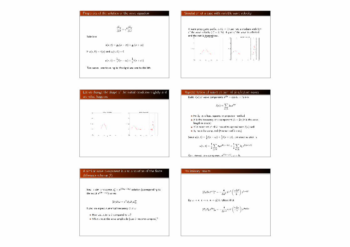
Simulation of a case with variable wave velocity

A wave propagates perfectly (C = 1) and hits a medium with 1/4of the wave velocity (C = 0.25). A part of the wave is reectedand the rest is transmitted.

Let us change the shape of the initial condition slightly andsee what happens

Representation of waves as sum of sine/cosine waves

Build I (x) of wave components e ikx = cos kx + i sin kx :

I (x) ≈∑

k∈Kbke

ikx

Fit bk by a least squares or projection method

k is the frequency of a component (λ = 2π/k is the wavelength in space)

K is some set of all k needed to approximate I (x) well

bk must be computed (Fourier coecients)

Since u(x , t) = 12 I (x − ct) + 1

2 I (x + ct), the exact solution is

u(x , t) =1

2

∑

k∈Kbke

ik(x−ct) +1

2

∑

k∈Kbke

ik(x+ct)

Our interest: one component e i(kx−ωt), ω = kc

A similar wave component is also a solution of the nitedierence scheme (!)

Idea: a similar discrete unq = e i(kxq−ωtn) solution (corresponding to

the exact e i(kx−ωt)) solves

[DtDtu = c2DxDxu]nq

Note: we expect numerical frequency ω 6= ω

How accurate is ω compared to ω?

What about the wave amplitude (can ω become complex)?

Preliminary results

[DtDteiωt ]n = − 4

∆t2sin2

(ω∆t

2

)e iωn∆t

By ω → k , t → x , n→ q) it follows that

[DxDxeikx ]q = − 4

∆x2sin2

(k∆x

2

)e ikq∆x

Insertion of the numerical wave component

Inserting a basic wave component u = e i(kxq−ωtn) in the schemerequires computation of

[DtDteikxe−iωt ]nq = [DtDte

−iωt ]ne ikq∆x

= − 4

∆t2sin2

(ω∆t

2

)e−iωn∆te ikq∆x

[DxDxeikxe−iωt ]nq = [DxDxe

ikx ]qe−iωn∆t

= − 4

∆x2sin2

(k∆x

2

)e ikq∆xe−iωn∆t

The equation for ω

The complete scheme,

[DtDteikxe−iωt = c2DxDxe

ikxe−iωt ]nq

leads to an equation for ω (which can readily be solved):

sin2(ω∆t

2

)= C 2 sin2

(k∆x

2

), C =

c∆t

∆x(Courant number)

Taking the square root:

sin

(ω∆t

2

)= C sin

(k∆x

2

)

The numerical dispersion relation

Can easily solve for an explicit formula for ω:

ω =2

∆tsin−1

(C sin

(k∆x

2

))

Note:

This ω = ω(k , c,∆x ,∆t) is the numerical dispersion relation

Inserting ekx−ωt in the PDE leads to ω = kc , which is theanalytical/exact dispersion relation

Speed of waves might be easier to imagine:

Exact speed: c = ω/k,Numerical speed: c = ω/k

We shall investigate c/c to see how wrong the speed of anumerical wave component is

The special case C = 1 gives the exact solution

For C = 1, ω = ω

The numerical solution is exact (at the mesh points),regardless of ∆x and ∆t = c−1∆x!

The only requirement is constant c

The numerical scheme is then a simple-to-use analyticalsolution method for the wave equation

Computing the error in wave velocity

Introduce p = k∆x/2(the important dimensionless spatial discretization parameter)

p measures no of mesh points in space per wave length inspace

Shortest possible wave length in mesh: λ = 2∆x ,k = 2π/λ = π/∆x , and p = k∆x/2 = π/2 ⇒ p ∈ (0, π/2]

Study error in wave velocity through c/c as function of p

r(C , p) =c

c=

2

kc∆tsin−1(C sin p) =

2

kC∆xsin−1(C sin p) =

1

Cpsin−1 (C sin p)

Can plot r(C , p) for p ∈ (0, π/2], C ∈ (0, 1]

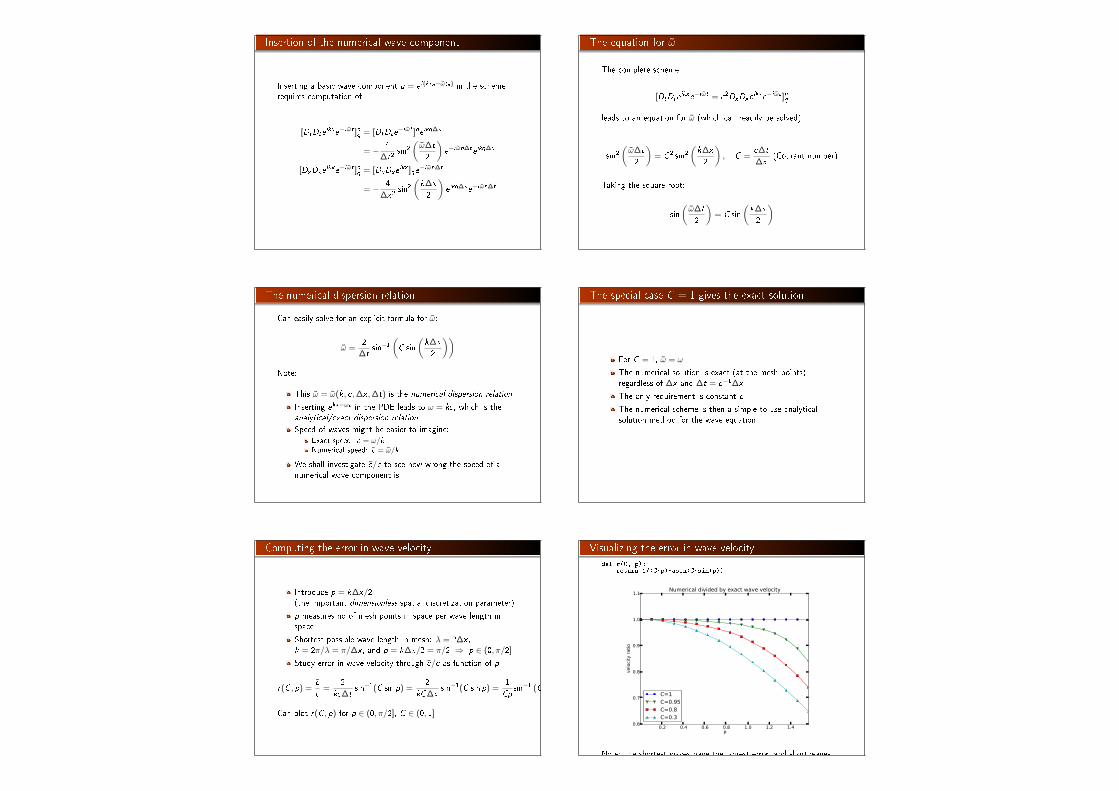
Visualizing the error in wave velocity

def r(C, p):return 1/(C*p)*asin(C*sin(p))

0.2 0.4 0.6 0.8 1.0 1.2 1.4p

0.6

0.7

0.8

0.9

1.0

1.1

velo

city

ratio

Numerical divided by exact wave velocity

C=1C=0.95C=0.8C=0.3

Note: the shortest waves have the largest error, and short wavesmove too slowly.

Taylor expanding the error in wave velocityFor small p, Taylor expand ω as polynomial in p:

>>> C, p = symbols('C p')>>> rs = r(C, p).series(p, 0, 7)>>> print rs1 - p**2/6 + p**4/120 - p**6/5040 + C**2*p**2/6 -C**2*p**4/12 + 13*C**2*p**6/720 + 3*C**4*p**4/40 -C**4*p**6/16 + 5*C**6*p**6/112 + O(p**7)

>>> # Drop the remainder O(...) term>>> rs = rs.removeO()>>> # Factorize each term>>> rs = [factor(term) for term in rs.as_ordered_terms()]>>> rs = sum(rs)>>> print rsp**6*(C - 1)*(C + 1)*(225*C**4 - 90*C**2 + 1)/5040 +p**4*(C - 1)*(C + 1)*(3*C - 1)*(3*C + 1)/120 +p**2*(C - 1)*(C + 1)/6 + 1

Leading error term is 16(C 2 − 1)p2 or

1

6

(k∆x

2

)2

(C 2 − 1) =k2

24

(c2∆t2 −∆x2

)= O(∆t2,∆x2)

Example on eect of wrong wave velocity (1)

Smooth wave, few short waves (large k) in I (x):

Example on eect of wrong wave velocity (1)

Not so smooth wave, signicant short waves (large k) in I (x):

Stability

sin

(ω∆t

2

)= C sin

(k∆x

2

)

Exact ω is real

Complex ω will lead to exponential growth of the amplitude

Stability criterion: real ω

Then sin(ω∆t/2) ∈ [−1, 1]

k∆x/2 is always real, so right-hand side is in [−C ,C ]

Then we must have C ≤ 1

Stability criterion:

C =c∆t

∆x≤ 1

Why C > 1 leads to non-physical waves

Recall that right-hand side is in [−C ,C ]. Then C > 1 means

sin

(ω∆t

2

)

︸ ︷︷ ︸>1

= C sin

(k∆x

2

)

| sin x | > 1 implies complex x

Here: complex ω = ωr ± i ωi

One ωi < 0 gives exp(i · i ωi ) = exp(−ωi ) and exponentialgrowth

This wave component will after some time dominate thesolution give an overall exponentially increasing amplitude(non-physical!)

Extending the analysis to 2D (and 3D)

u(x , y , t) = g(kxx + kyy − ωt)

is a typically solution of

utt = c2(uxx + uyy )

Can build solutions by adding complex Fourier components of theform

e i(kxx+kyy−ωt)

Discrete wave components in 2D

[DtDtu = c2(DxDxu + DyDyu)]nq,r

This equation admits a Fourier component

unq,r = e i(kxq∆x+ky r∆y−ωn∆t)

Inserting the Fourier component into the dicrete 2D wave equation,and using formulas from the 1D analysis:

sin2(ω∆t

2

)= C 2

x sin2 px + C 2

y sin2 py

where

Cx =c∆t

∆x, Cy =

c∆t

∆y, px =

kx∆x

2, py =

ky∆y

2

Stability criterion in 2D

Ensuring real-valued ω requires

C 2x + C 2

y ≤ 1

or

∆t ≤ 1

c

(1

∆x2+

1

∆y2

)−1/2

Stability criterion in 3D

∆t ≤ 1

c

(1

∆x2+

1

∆y2+

1

∆z2

)−1/2

For c2 = c2(x) we must use the worst-case valuec =

√maxx∈Ω c2(x) and a safety factor β ≤ 1:

∆t ≤ β 1c

(1

∆x2+

1

∆y2+

1

∆z2

)−1/2

Numerical dispersion relation in 2D (1)

ω =2

∆tsin−1

((C 2x sin

2 px + C 2y sin

py

) 12

)

For visualization, introduce k =√

k2x + k2y and θ such that

kx = k sin θ, ky = k cos θ, px =1

2kh cos θ, py =

1

2kh sin θ

Also: ∆x = ∆y = h. Then Cx = Cy = c∆t/h ≡ C .

Now ω depends on

C reecting the number cells a wave is displaced during a timestep

kh reecting the number of cells per wave length in space

θ expressing the direction of the wave

Numerical dispersion relation in 2D (2)

c

c=

1

Ckhsin−1

(C

(sin2(

1

2kh cos θ) + sin2(

1

2kh sin θ)

) 1

2

)

Can make color contour plots of 1− c/c in polar coordinates withθ as the angular coordinate and kh as the radial coordinate.

Numerical dispersion relation in 2D (3)

0.9450.8700.7950.7200.6450.5700.4950.4200.3450.270

erro

r in

wav

e ve

loci

ty