finite element modelling of shielded metal arc welding · this study involved the modelling and...
TRANSCRIPT

Finite Element Modelling of Shielded Metal Arc
Welding
By
M Cronje
Thesis presented at the University of Stellenbosch in
partial fulfilment of the requirements for the degree of
Master of Science in Mechanical Engineering
Department of Mechanical Engineering
Stellenbosch University
Private Bag X1, 7602 Matieland, South Africa
Study leader: Mr K. van der Westhuizen
Dr A.B. Taylor
December 2005

ii
Copyright © 2005 University of Stellenbosch
All rights reserved

iii
DECLARATION
I, the undersigned, hereby declare that the work contained in this thesis is my
own work and that I have not previously in its entirety or in part submitted it at
any university for a degree.
Signature:……………………………………………..
M. Cronje
Date:……………………………………………….…..

iv
ABSTRACT
Finite Element Modelling of Shielded Metal Arc Welding
M. Cronje
Department of Mechanical Engineering
Stellenbosch University
Private Bag X1, 7602 Matieland, South Africa
Thesis: MScEng (Mech) December 2005
This study involved the modelling and verification of the Shielded Metal
Arc Welding of mild steel with the focus on displacement and temperature
distribution prediction of welded plates.
The project was divided into three phases namely; the literature survey
into finite element modelling of welding processes, the modelling of a welding
process and verification of the modelling with experimental results.
A working welding model was created using a commercial finite element
software package with the capabilities to model welding processes. The welding
model was systematically developed from a two-dimensional model into a three-
dimensional full physics process model. Experimental measured welding heat
input parameters were applied in the model, temperature dependent material
properties were applied and actual structural restraints from the experiments
were modelled.
Displacement and temperature distributions were measured on mild steel
plates welded with the Shielded Metal Arc Welding process. The plate
temperature was measured at various locations with K-type thermocouples spot
welded onto the plates. Plate deformation was measured at various stages of the
manufacturing process. Tendencies in plate displacement were investigated with
a change in certain welding parameters. The finite element model was verified
and good correlations were found, especially for the temperature distribution in
the welded plates.

v
UITREKSEL
Eindige Element Modellering van Geskermde Metaal Vonk Sweis
M. Cronje
Departement Meganiese Ingenieurswese
Universiteit van Stellenbosch
Privaatsak X1, 7602 Matieland, Suid-Afrika
Tesis: MScIng (Meg) Desember 2005
Hierdie studie behels die modellering en verifiëring van Geskermde
Metaal Vonk Sweis van sagte staal met die fokus gemik op die verplasing en
temperatuur verspreiding van gesweiste plate.
Die projek was opgedeel in drie fases naamlik; die literatuurstudie van die
eindige element modellering van sweisprosesse, die modellering van ‘n
sweisproses en die verifiëring van die model met eksperimentele resultate.
’n Werkende model was geskep met die gebruik van ‘n kommersiële
eindige element pakket met die vermoë om sweisprosesse te modelleer. Die
sweis model was sistematies ontwikkel vanaf ’n twee-dimensionele model na ’n
volledige-proses drie-dimensionele model. Eksperimentele gemete sweis hitte-
inset parameters was toegepas in die model, temperatuur afhanklike materiaal
eienskappe en die strukturele beperkings van die eksperiment was gemodelleer.
Verplasing en temperatuur verspreiding van sagte staal plate, gesweis
met die Geskermde Metaal Vonk Sweisproses, was gemeet. Die plaat
temperatuur was gemeet by verskeie liggings met K-tipe termokoppels wat
gepuntsweis is op die plaat. Plaat verplasing was gemeet by verskillende
stadiums van die vervaardigingsproses. Tendense in plaat verplasing was
ondersoek met verandering in sekere sweis veranderlikes. Die resultate van die
eindige element metode was geverifieer en goeie korrelasie was gevind, veral vir
die temperatuur verspreiding in gesweiste plate.

vi
ACKNOWLEDGEMENTS
First of all, I would like to thank Dr Taylor and Mr Van der Westhuizen for
their persistent motivation, visionary guidance and continual support. You
believed in this project where others doubted. Your inspiration made this project
possible.
Many thanks to the modelling teams of Stellenbosch Automotive
Engineering (CAE) and IMEC (Belgium) who were always nearby and willing to
assist in the many challenges faced in this project. The free advice and support
you have given cannot be valued and I will always be in your debt.
The staff and artisans at SMD for all the mechanical services and
performing of the experiments, especially Mr Van der Vinne and Van der Berg for
their patience, support and advise which were unmistakably the backbone of the
project. Mr Cobus Zietsman who made everything possible and was never to
busy to give a helping hand.
Many friends, co-students and colleagues for their support and
understanding.
Lastly, my family who provided continuous support, love and motivation
and a very special lady friend, Hannelie, for the support and motivation during the
project.

vii
DEDICATIONS
I dedicate this to my father, you made this all possible.
viii
TABLE OF CONTENTS
DECLARATION ................................................................................................... iii
ABSTRACT.......................................................................................................... iv
UITREKSEL.......................................................................................................... v
ACKNOWLEDGEMENTS .................................................................................... vi
DEDICATIONS ................................................................................................... vii
TABLE OF CONTENTS......................................................................................viii
LIST OF FIGURES .............................................................................................. xi
LIST OF TABLES............................................................................................... xiv
NOMENCLATURE.............................................................................................. xv
LIST OF ABBREVIATIONS ...............................................................................xvii
1 INTRODUCTION ...........................................................................................1
2 WELDING......................................................................................................3
2.1 Background of Welding...........................................................................3
2.2 Physics of Welding .................................................................................4
2.2.1 Heat Transfer ..................................................................................4
2.3 Welding Processes.................................................................................5
2.3.1 Shielded Metal Arc Welding ............................................................6
2.3.2 Gas Metal Arc Welding....................................................................6
2.3.3 Gas Tungsten Arc Welding..............................................................7
2.4 Welding Distortions.................................................................................8
2.4.1 Control of Welding Distortions .........................................................9
2.4.2 Calculation of Welding Distortions.................................................13
2.5 Metallurgy of Welding ...........................................................................14
2.5.1 Low Carbon Steels ........................................................................14
2.6 Conclusion............................................................................................16
3 FINITE ELEMENT METHOD: APPLICATION TO WELDING......................17
3.1 Introduction...........................................................................................17

ix
3.2 Finite Element Analysis of Welding ......................................................17
3.2.1 Two-dimensional vs. Three-dimensional Modelling .......................18
3.2.2 Thermal and Structural Analysis....................................................21
3.2.3 Prediction of Welding Distortion ....................................................21
3.2.4 Modelling Assumptions..................................................................22
3.2.5 Applied Heat Source......................................................................23
3.2.6 Time Step Estimate .......................................................................27
3.2.7 Boundary Heat Loss Conditions ....................................................29
3.3 Material Properties ...............................................................................30
3.3.1 Conductivity...................................................................................30
3.3.2 Specific Heat .................................................................................31
3.3.3 Yield Strength................................................................................33
3.3.4 Alternative Material Property Methods...........................................34
3.4 Conclusion............................................................................................35
4 EXPERIMENTS...........................................................................................37
4.1 Introduction...........................................................................................37
4.2 Experimental Set Up.............................................................................38
4.3 Effect of Restraints ...............................................................................40
4.3.1 Introduction....................................................................................40
4.3.2 Results ..........................................................................................42
4.4 Effect of Plate Thickness ......................................................................44
4.4.1 Introduction....................................................................................44
4.4.2 Results ..........................................................................................46
4.5 Effect of Current Setting .......................................................................54
4.5.1 Introduction....................................................................................54
4.5.2 Results ..........................................................................................54
4.6 Temperature Measurement ..................................................................58
4.6.1 Introduction....................................................................................58
4.6.2 Results ..........................................................................................60
4.7 Conclusion on Experiments ..................................................................64
x
5 MODELLING OF WELDING EXPERIMENTS .............................................66
5.1 Introduction...........................................................................................66
5.2 Weld Modelling in MSC.Marc ...............................................................67
5.3 Weld Model Preparation .......................................................................67
5.3.1 Geometry and Element Meshing ...................................................67
5.3.2 Material Properties ........................................................................68
5.3.3 Boundary Conditions .....................................................................69
5.3.4 Element Activation/De-Activation ..................................................71
5.3.5 Coupled and Uncoupled Analysis..................................................72
5.4 Numerical Results ................................................................................73
5.4.1 Thermal Results ............................................................................73
5.4.2 Structural Results ..........................................................................75
5.4.3 Experiment vs. FEM ......................................................................81
6 CONCLUSION.............................................................................................83
6.1 Recommendations................................................................................85
REFERENCES ...................................................................................................86
APPENDIX A ......................................................................................................91
A.1 Calculation of Natural Convection ........................................................91
APPENDIX B EXPERIMENTAL RESULTS ........................................................95
B.1 Effect of Restraints ...............................................................................95
B.2 Effects of Plate Thickness ....................................................................99
B.3 Effect of Heat Input.............................................................................103
APPENDIX C EXPERIMENTAL TEMPERATURE RESULTS ..........................107

xi
LIST OF FIGURES
Figure 2-1: Shielded metal arc welding (SMAW) ..................................................6
Figure 2-2: Gas metal arc welding (GMAW). ........................................................7
Figure 2-3: Gas tungsten arc welding (GTAW). ....................................................8
Figure 2-4: Welded plate distortions (Faure, undated)..........................................9
Figure 2-5: Welding distortion in multiple-run welding (Faure, undated) .............10
Figure 2-6: The back-step method (Faure, undated). .........................................10
Figure 2-7: Angular distortion control with symmetrical welds (Faure, undated). 11
Figure 2-8: Thermal management techniques applied to welding.......................12
Figure 2-9: Effect of thermal management techniques on HAZ (Jung, 2004). ....13
Figure 2-10: Phase diagram for carbon steel during welding..............................15
Figure 3-1: Illustration of the 2D planes in the modelling of welded plates. ........19
Figure 3-2: Gaussian distributed volume heat source (Eagar, et al., 1983). .......25
Figure 3-3: Double ellipsoidal density heat source (Francis, 2002).....................26
Figure 3-4: Negative temperature effect due to small initial time step estimate
(MSC.Marc Manual, 2005)...........................................................................27
Figure 3-5: Temperature dependant thermal conductivity for mild steel (Goldak,
et al., 1984)..................................................................................................31
Figure 3-6: Specific heat for mild steel (British Iron and Steel Research
Association Metallurgy, 1953)......................................................................32
Figure 3-7: Zhu and Chao (2002) yield stress approximation for an Al alloy.......34
Figure 3-8: Thermal conductivity for 300WA and Common Steel (British Iron and
Steel Research Association Metallurgy, 1953). ...........................................35
Figure 4-1: Measurement of welded plates with dial gauge on measuring table.39
Figure 4-2: Distortion and plastic strain vs. clamping (www.esi-group.com) .......40
Figure 4-3: Clamping configurations investigated in experiments.......................41
Figure 4-4: Excessive distortion of welded plates due to misalignment. .............42
Figure 4-5: Welding distortion theory due to plate misalignment. .......................43

xii
Figure 4-6: Transverse displacement in middle of plate after welding but before
the removal of the clamping for different clamp settings..............................44
Figure 4-7: Transverse displacement in the middle of the pate after removal of
clamps. ........................................................................................................45
Figure 4-8: Order of the removal of clamps. .......................................................45
Figure 4-9: Welding speed vs. heat input per unit thickness for welding of plates
with different thickness. ...............................................................................49
Figure 4-10: Point of maximum deflection for welded plates in the experiments.50
Figure 4-11: Transverse displacement for different thickness after removal of
clamps. ........................................................................................................51
Figure 4-12: Final longitudinal displacement for different plate thickness, after
removal of all clamping. ...............................................................................52
Figure 4-13: Transverse displacement for different plate thickness with only
reference clamp on plates............................................................................53
Figure 4-14: Displacement of plates with reference clamp: longitudinal
displacement................................................................................................53
Figure 4-15: Transverse displacement for different current settings after clamp
removal. .......................................................................................................56
Figure 4-16: Final displacement for different current settings, longitudinal
displacement................................................................................................57
Figure 4-17: Thermocouple locations on welded plates......................................59
Figure 4-18: Thermocouple spot-welded to mild steel plate................................60
Figure 4-19: Maximum temperatures of thermocouples at distance 20 mm from
weld. ............................................................................................................62
Figure 4-20: Comparison of maximum temperatures in transverse line with
analytical solution. .......................................................................................63
Figure 4-21: Temperature distribution at distance 20 mm from weld in centre of
plate for three different experiments. ...........................................................63
Figure 5-1: Temperature distribution for different thickness, 50 mm from weld. .74
Figure 5-2: Transverse displacement for different thickness after clamp removal
(FEM)...........................................................................................................77

xiii
Figure 5-3: Longitudinal displacement for different thickness after clamp removal
(FEM)...........................................................................................................77
Figure 5-4: Weld pool size in FEA for 70 A model. .............................................79
Figure 5-5: Transverse displacement for 70A welding. .......................................80
Figure 5-6: Longitudinal displacement for 70A welding, 55mm from weld. .........80
Figure A-1: Convective heat transfer coefficient of heated horizontal plate. .......94

xiv
LIST OF TABLES
Table 3-1: Chemical composition for 300WA and Common Steel. .....................35
Table 4-1: Values of the welding parameters used in the experiments...............38
Table 4-2: Average welding process parameters for different plate thickness. ..46
Table 4-3: Energy input parameters for different plate thickness........................47
Table 4-4: Average welding process parameters for different current settings. ..55
Table 4-5: Average energy input parameters for different current settings. ........55
Table 4-6: Distance of thermocouple measuring point to centre of weld.............61
Table 5-1: Experimentally determined heat source parameters..........................70
Table 5-2: Volume heat source dimension used in FEA for different weld current
settings. .......................................................................................................78

xv
NOMENCLATURE
c - specific heat [J/kg.°C]
d - weld bead width [m]
E - Young’s modulus [GPa]
El - energy per unit length [J/mm]
g - gravitational acceleration [m/s²]
h - plate thickness [mm]
hc - convection heat transfer coefficient [W/m².°C]
hr - radiation heat transfer coefficient [W/m².°C]
I - electric current [A]
k - thermal conductivity [W/m.°C]
L - characteristic length [mm]
Nu - Nusselt number
P - power [W]
Ra - Rayleigh number
T - temperature [°C]
Tm - melting point temperature [°C]
t - time [s]
V - voltage [V]
v - welding speed [m/s]
Q - heat input [W]
q - heat flux [W/m²]
x,y,z - spatial coordinates [m]
α - thermal diffusivity [m²/s]
β - thermal coefficient of volume expansion [K-1]

xvi
ηarc - arc efficiency
ρ - density [kg/m³]
ν - kinematic viscosity [m²/s]

xvii
LIST OF ABBREVIATIONS
AC - Alternating current
DC - Direct current
EMF - Electromotive force
FE - Finite element
FEA - Finite element analysis
FEM - Finite element method
GMAW - Gas metal arc welding
GTA - Gas tungsten arc
HAZ - Heat affected zone
MIG - Metal inert gas
MSC - Macneal-Schwendler Corporation
NASA - National Aeronautical and Space Administration
NASTRAN - NASA Structural Analysis Program
SMAW - Shielded metal arc welding
TIG - Tungsten inert gas

1
1 INTRODUCTION
South Africa’s automotive component manufacturing industry is renowned
internationally for its expertise, flexibility and rapid growth in production. The
country has vast resources and already counts among the twenty largest vehicle
manufacturers in the world and is fast increasing its vehicle-manufacturing
capacity. However, South Africa is not at the leading edge of technological
development of manufacturing in the automotive industry (Lourens, 2002). South
Africa competes against the world: whether it is Mexico, China or Australia.
Therefore it is critical to improve and develop manufacturing technology that will,
if properly applied, improve productivity, add value to products and reduce waste.
The implementation of numerical techniques to model manufacturing processes
has the advantage of improving the product, perfecting the process, reducing
scrap rates, reducing product realization costs and improves the efficiency of the
manufacturing process. The graphical display of the modelling software available
also gives insight to the mechanics of the manufacturing process.
Modelling can be used as a tool in many stages of the life of a product: from a
concept evaluation tool to manufacturing analysis tool. There is a big market for
this kind of analysis in an industry where there are still heavily relied on extensive
testing and development. This primitive approach to production is not only
expensive but also time consuming.
The complex nature of the welding process causes difficulty in analysing and
modelling by numerical methods. These complexities include: temperature
dependent material properties, non-linear boundary conditions, moving heat
sources, phase changes and transformations, complex residual stress states and
the difficulties of making experimental measurements at high temperatures. In
addition to these complexities, finite element modelling of the weld process must
2
include complex thermo-mechanical interactions, filler metal deposit and moving
heat sources.
The objectives for the thesis could be summarised as:
• Create a thermal-mechanical finite element analysis of the welding
process.
• Perform welding experiments to determine the plate deflections and
temperature distribution in mild steel plates during shielded metal arc
welding (SMAW).
• Evaluate the verification of experimental and numerical results.
• Determine the parameters necessary for an accurate and effective weld
simulation and the sensitivity of modelling parameters on the results.
In Chapter 2 and 3 the literature survey done on welding and the application of
the finite element method (FEM) in weld modelling are discussed. The modelling
assumptions and techniques used by previous researchers used in the thesis are
discussed in Chapter 3. The experimental setup and results are discussed in
Chapter 4 with all the experimental results in Appendix B and C. The description
of the weld modelling is in Chapter 5 and the verification of numerical results with
experimental results is in Chapter 6. Conclusions and recommendations are
made in Chapter 7.

3
2 WELDING
2.1 Background of Welding
Although welding is considered a relatively new process as practiced today, its
origins can be traced to ancient times. Around 1000 B.C. the Egyptians and
others in the Mediterranean area learned to accomplish forge welding.
Blacksmiths from the Middle Ages developed the art of welding by hammering
metals to a high level of maturity.
It was not until the 1800s that the technological foundations of modern welding
were established when the electric arc and acetylene gas was discovered. The
development of electrical generators in the mid 1800s made electrical power
became available in amounts sufficient to sustain arc welding. At the turn of the
19th century, carbon arc welding had become a popular commercial process for
joining metals, but the process was still limited. Welding with a metal electrode
was developed and had the unique feature that the electrode added filler metal to
the welding joint (Groover, 1999).
Arc welding with a fusible electrode, the most important of the fusion processes,
was more complex in character and developed more slowly. In the early stages
of this development fusion welding was used primarily as a means of repairing
worn or damaged metal parts, but during the First World War, research was
initiated into the acceptability of the technique as a primary means of joining steel
plate and prototype structure were made.
Welding has been employed at an increasing rate for its advantages in design
flexibility, cost savings, reduced overall weight and enhanced structural
performance.

4
2.2 Physics of Welding
There are two main categories for welding: fusion and solid phase welding
processes. In fusion welding, two edges or surfaces to be joined are heated to
the melting point and, where necessary, molten filler metal is added to fill the joint
gap. For solid phase welding, two clean, solid metal surfaces are brought into
sufficiently close contact for a metallic bond to be formed. Solid phase welding
can be accomplished at temperatures as low as room temperature.
By using a heat source with sufficient power it is possible to fuse through a
complete section of very thick plate. The weld pool produced is difficult to control
and the heat affected zone (HAZ) of such welds has a relatively coarse grain,
adversely affecting the mechanical properties of the steel (Lancaster, 1965).
2.2.1 Heat Transfer
An understanding of the nature of heat transfer is essential for the proper
appreciation of the heat effect of fusion welding. Heat transfer theory can indicate
the minimum heat input rate to form a weld of any given width, and the essential
variables which govern the heating rate and cooling rate in the heat affected
zone and the weld metal.
The electric arc heat source is known as a surface heat source, which applies
heat over a small area on the metal surface. In most fusion welding a continuous
moving source is used. The continuous moving source has a special
characteristic: once steady conditions have been achieved, the temperature
distribution relative to the heat source is stationary. This condition is known as
the quasi-stationary state and in most cases it is convenient in developing
equations regarding the source as stationary and the heat flow medium (the work
piece) as moving. Equation 2-1 shows the conduction of heat in a homogeneous
isotropic solid in terms of rectangular co-ordinates (Lancaster, 1965):

5
01
2
2
2
2
2
2
=∂
∂−
∂
∂+
∂
∂+
∂
∂
t
T
z
T
y
T
x
T
α Equation 2-1
The power of the welding process is the product of the current I and voltage V
passing through the arc. The power is converted to heat, but due to convection,
conduction, radiation and spatter, heat losses occur. The temperature attainable
in an arc is limited by heat leakage rather than by a theoretical limit (Phillips,
1968). The effect of heat losses is expressed by the arc efficiency coefficient,
ηarc, in the calculation of the welding power.
VIP arcη= Equation 2-2
Welding arcs are usually maintained between an electrode and a plate work
piece. Such an arc is constricted at the rod and spreads out towards the plate.
The column temperature is highest where it is most constricted, in this instance
near the electrode. Having a clear understanding of the temperature and heat
flux distribution in an arc is very important for the load application in weld
modelling. An accurate representation of the thermal flux in the finite element
method (FEM) software package will help with more accurate and reliable
results.
2.3 Welding Processes
Arc welding is a fusion process in which coalescence of the metals is achieved
by the heat from an electric arc between an electrode and the work. Filler metal
is added in most welding processes to increase the volume and strength of the
weld joint. A pool of molten metal, consisting of base and filler metal is formed
near the tip of the electrode. As the electrode is moved along the joint, the molten
metal solidifies in its wake. In this section some of the common arc welding
processes that use consumable electrodes will be discussed.

6
2.3.1 Shielded Metal Arc Welding
Shielded metal arc welding (SMAW) use an electrode consisting of a filler metal
rod coated with chemicals that provide flux and shielding (Figure 2-1). The filler
metal used in the rods must be compatible with the metal to be welded, the
composition usually close to that of the base metal. Currents typically used in
SMAW range between 30 and 300 A at voltages from 15 to 45 V. Selection of the
power parameters depends on the metals being welded, electrode type and
length, and depth of penetration.
Shielded metal arc welding is performed manually and the equipment is portable
and low cost, making SMAW highly versatile. Base metals that could be welded
with SMAW include steels, stainless steels, cast irons and certain non-ferrous
alloys. The disadvantage of SMAW is the use of consumable electrode sticks
and needs to be replaced at regular intervals. The level of the current used is
also a limitation because the electrode length varies during the operation and
affects the heat resistance of the electrode.
Figure 2-1: Shielded metal arc welding (SMAW)
2.3.2 Gas Metal Arc Welding
Gas metal arc welding (GMAW) is an arc welding process in which the electrode
is a consumable bare wire and shielding is accomplished by flooding the arc with
a gas. The bare wire is fed continuously from a spool through the welding gun.

7
The GMAW have various advantages over SMAW, which make it popular in
fabrication operations. The combination of bare electrode wire and shielding gas
eliminates the formation of slag on the weld bead and thus precludes the use of
manual cleaning after welding. This makes GMAW popular for multi-pass
welding. Because GMAW is continuously wire fed, the electrode do not need
replacing at regular intervals such as in the case of SMAW, making this process
suitable for automated welding. The utilization of electrode material is higher than
with SMAW.
Figure 2-2: Gas metal arc welding (GMAW).
2.3.3 Gas Tungsten Arc Welding
Gas tungsten arc welding is an arc welding process that uses a non-consumable
tungsten electrode and an inert gas for arc shielding (Figure 2-3). The term TIG
(tungsten inert gas) welding and WIG (W is the chemical symbol for tungsten)
welding are often applied to this process. The GTAW can be implemented with or
without filler metal. When filler metal is used, it is added to the weld pool from a
separate rod or wire. The typical shielding gases used are argon, helium or a
mixture of these gases.
Advantages of GTAW in the applications to which it is suited includes high-quality
welds, no weld spatter because no filler metal is transferred across the arc and
little or no post weld cleaning because no flux is used. The welding costs of
GTAW are higher than SMAW or GMAW because specialized equipment is

8
used, lower manual speed and the use of an inert gas. GTAW will be typically
applied where a technical advantage is needed (Lancaster, 1965).
Figure 2-3: Gas tungsten arc welding (GTAW).
2.4 Welding Distortions
Welding distortions due to a weld in a plate arise primarily because the strip of
material which has been melted contracts on cooling down from melting point to
room temperature. Welding distortions can be separated into three types of
distortions: angular, longitudinal and transverse distortion.
The contraction of weld metal as it cools after deposition causes shrinkage that
takes place simultaneously in all directions, and therefore it causes several types
of distortion as illustrated in Figure 2-4. The levels of welding distortions depend
mostly on the heat input and the material thickness (Luo, Ishiyama, Murakawa,
1999). Material type also determines the extent of welding deformation.
If the contraction of the weld was unhindered, the longitudinal contraction of the
weld would be equal to αTm where α is the thermal expansion and Tm the melting
temperature. Assuming only elastic deformation the corresponding stress would
be EαTm where E is the Young’s modulus of the material. The value of EαTm is
greater than the elastic limit, so that plastic deformation of the weld takes place
during cooling and the residual stress in the weld exceeds the elastic limit.

9
Figure 2-4: Welded plate distortions (Faure, undated)
In multi-pass welding, the first run in a butt weld pulls the plates together when
shrinkage occurs (Figure 2-5). The second run is restrained by the first, which
has to be compressed before plates can move together. The pull at the top and
the push at the bottom of the weld give rise to angular distortion. A number of
superimposed runs trying to contract, along with the initial shrinkage of the first
run, cause a transverse shrinkage of the joint. Similar forces act along the length
of the joint, thus producing lengthwise distortion and longitudinal shrinkage.
2.4.1 Control of Welding Distortions
Distortion due to welding has been regarded as a critical issue and has led to the
development of various techniques and guidelines to minimize these distortions.
In general, most of the distortion mitigation techniques have been developed
according to theoretical, mathematical and generally accepted knowledge from
experience or analogy. Faure had suggested three rules for the prevention and
control of distortions (Faure, undated):
• Reduce the effective shrinkage force.
• Utilise shrinkage forces to reduce distortion.
• Balance shrinkage forces with other forces.
10
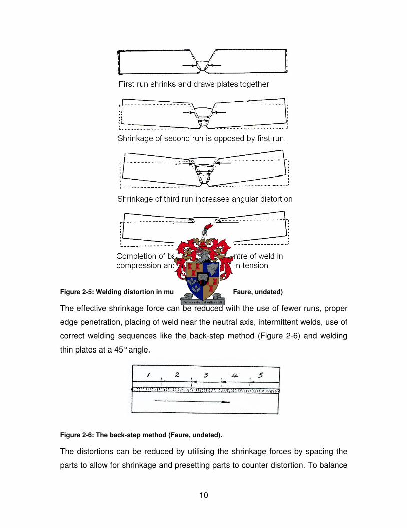
Figure 2-5: Welding distortion in multiple-run welding (Faure, undated)
The effective shrinkage force can be reduced with the use of fewer runs, proper
edge penetration, placing of weld near the neutral axis, intermittent welds, use of
correct welding sequences like the back-step method (Figure 2-6) and welding
thin plates at a 45° angle.
Figure 2-6: The back-step method (Faure, undated).
The distortions can be reduced by utilising the shrinkage forces by spacing the
parts to allow for shrinkage and presetting parts to counter distortion. To balance

11
shrinkage forces with other forces, a proper welding sequence can be used to
counter shrinkage force (Figure 2-7). Other techniques to reduce distortion and
residual stresses are tack welding to prevent movement of parts, peening for
stress relieving, using of heat to straighten parts, use of jigs and fixtures,
machining and stress-relieving heat treatment.
Figure 2-7: Angular distortion control with symmetrical welds (Faure, undated).
The use of optimised welding sequences changes the distribution of the residual
stresses but does not change the maximum residual stress. High residual stress
is formed in a region around the weld line irrespective of the welding sequence,
however, the welding sequence mainly effect the distortions in the weldment
(Kadivar, Jafarpur, Baradaran, 2000).
Distortion control becomes more difficult the larger and more complex the
structure becomes. It is advisable to attack the overall accuracy control problem
by starting at the end of the fabrication sequence and working backwards.
Current procedures to reduce welding distortion can be divided according to the
three stages at which it takes place:
• Pre-welding strategies such as fix devices, etc.
• In-process corrections such as speed adjustments, change of planned
weld sequence, etc.
• Post-welding adjustments such as flame heating.
It was suggested that better control of certain welding variables would eliminate
the conditions that promoted distortion (Tsai, Park, Cheng, 1999). This included

12
the reduction of fillet welds size and length, high speed welds, low heat input
welding process, intermittent welds, back stepping (Figure 2-6) and balancing
heat about the plate’s neutral axis in butt joint welding.
Thermal management techniques have been applied for distortion control of
welded plates. Two common techniques investigated (Figure 2-8) were the gas
tungsten arc (GTA) and heat sinking (Jung, Tsai, 2004) procedures. The GTA
increased the HAZ by preheating. Heat sinking reduced the HAZ by applying a
cooling chamber beneath the welding area (Figure 2-9).
Figure 2-8: Thermal management techniques applied to welding.
Jung and Tsai used plasticity-based distortion analysis (PDA) and elastic-plastic
analysis to obtain stress and strains results in welded T-joints. It was found that
the heat sinking increased angular distortion and that GTA preheating reduced it.
A combination of GTA preheating and external restraining effectively reduced the
angular distortion. The reduction of angular distortion during GTA preheating was
not fully understood, since there was little difference between the results from
GTA preheating and no thermal management.

13
Figure 2-9: Effect of thermal management techniques on HAZ (Jung, 2004).
2.4.2 Calculation of Welding Distortions
Welding deformation reduces the accuracy of manufacturing and decreases
productivity due to the need for correction work. The minimization of distortions
from as early as the design stage will lead to higher quality of products as well as
higher productivity. Prediction of welding distortions through analytical and
numerical methods like empirical equations and FEA form an essential part in
manufacturing.
With the use of more expensive steels or other metals, like stainless steel, larger
welding deformations can occur due to the materials’ properties. It is important to
foresee forthcoming welding deformations and its extent to prevent costly repairs
of inaccurate welds. The methods for analytical approaches for determination of
welding deformations of several researchers had been investigated.
It was found that the welding deformations calculation methods of Okerblom,
Walter, Horst Pflug, Sparagen–Etinger and Blodgett, applied to calculate
deformations of welded samples, gave results that differ greatly (cited by
Audronis and Bendikas, 2003). Their studies looked at the results for longitudinal
contraction, longitudinal deflection on the plate’s plane, transversal contraction
and transversal deflection. These results were compared with FEA results.

14
The calculations proposed by the abovementioned researchers must be used
with caution. These formulas are capable of reliable predictions within the
limitations upon which it is based. Any change of parameters, which has not
been included, can lead to a calculation error. In many cases these calculations
may serve the purpose of predicting no more than the order of the magnitude of
welding distortions. The formulas are however not suitable for predicting
distortions of large structures (Moshaiov, Eagar, 1990).
A method based on the inherent strain theory combined with FEM for the
prediction of welding deformations was proposed by various researchers (Luo, et
al., 1999 and Jang, Lee, 2003). The equivalent forces and moments that would
result in the same deformations as in welding could be obtained by using the
inherent strain method. Using the obtained equivalent nodal loads, the welding
deformation could be calculated by elastic FE analysis.
2.5 Metallurgy of Welding
Welding has the ability to join various metals, both similar and dissimilar. The
joining bond is metallurgical rather than just mechanical, as with riveting and
bolting. Due to the intense heating and fast cooling of the weld material the
microstructure of the metal undergoes considerably changes.
This region is termed the heat affected zone (HAZ). In cold worked metals the
HAZ may have experienced recrystallization and grain growth and thus a
diminishment of strength, hardness and toughness. Upon cooling residual
stresses may form in this region, which weakens the joint (Callister, 1997).
2.5.1 Low Carbon Steels
The metal most widely used in welded fabrication is carbon steel containing up to
about 0.3% carbon (mild steel). This material undergoes only minor hardening in
the heat-affected zone of fusion welds and normally is welded without any pre- or
post welding heat treatment. Higher carbon steels are more difficult to weld,

15
except in the form of thin sheet or bar, because hardening of the weld and heat
affected zone may result in embrittlement and cracking. One undesirable feature
common to all ferrous materials welded is grain growth in the region near the
fusion boundary.
A welded joint consists out of a molten pool zone (MPZ), a fusion zone (FZ) and
a heat affected zone (HAZ). The HAZ is defined as the part of the metal that has
not been melted but whose material properties or microstructure has been
altered by the heat of the welding. This zone is indicated by region 4 to 1 in
Figure 2-10.
Figure 2-10: Phase diagram for carbon steel during welding.
In region 1 the temperatures were close to melting point. The heat treatment has
refined the grain structure and austenitic grain growth takes place. There is an
improvement in toughness of the mild steel. If the cooling rate is high, the
microstructure can readily change to martensite.

16
The heat from the welding process has raised the temperature in region 2 to just
above the lower critical point. At this temperature the ferrite remains unchanged,
but the pearlite is dissolved to austenite. Upon cooling, the carbon is precipitated
in the form of small globules of cementite in ferrite. This type of structure is
acceptable as it produces softness and good ductility. In region 3 the metal was
heated to just above 600 °C and consists of newly formed fine equiaxed grains of
ferrite and pearlite. This temperature region undergoes relieving of residual
stress. Temperatures below 450 °C remain unchanged.
2.6 Conclusion
A literature study was carried out to gather information on the welding process
and the mechanics of plate deformation during welding. Sequence welding and
thermal management techniques used in distortion control and prevention in
welded plates were discussed. The use of optimised welding sequences helps to
control welding distortion during welding but have no effect on the maximum
stress values. Thermal management techniques can be used to control the size
of the HAZ and reduce residual stresses through stress relieving.
Theoretical equations were obtained to be used in first order derivatives of the
experimental and modelling results. In these first order derivatives the
experimental and modelling results were compared with the theoretical results to
insure the validity of the results. The use of thermal management techniques and
other welding mitigation techniques were not studied in depth in the literature
survey and can be looked into in future studies. The causes and control of
welding fracture can also be investigated in future welding research.

17
3 FINITE ELEMENT METHOD: APPLICATION TO
WELDING
3.1 Introduction
The finite element method (FEM) is a computational technique used to obtain
approximate solutions of boundary value problems in engineering. The finite
element method is a way of getting a numerical answer to a specific problem. A
simple description of FEM is the cutting of a structure into several elements,
describing the behaviour of each element in a simple way, reconnecting the
elements at ”nodes” as if it were pins or drops of glue that held the elements
together.
A literature survey was done to look at the development and history of the finite
element method, the role of FEM in welding analysis and the effect of welding
and modelling parameters on the results. The survey focused on temperature
field estimation and welding deformation. Weld modelling guidelines on element
mesh, boundary conditions and material properties from the survey were applied
in the thesis.
3.2 Finite Element Analysis of Welding
The numerical modelling of welding can be used as design tool or manufacturing
analysis tool. As a design tool, FEM can be used to evaluate the feasibility of
designs as early as the concept phase. As a manufacturing analysis tool, for
fixed designs, different welding processes and sequences can be evaluated to
minimize welding distortion (Michelaris, DeBiccari, 1996).
Despite the success that had been demonstrated by researchers over the past
few decades of conduction heat flow models in predicting fusion weld sizes, base

18
metal temperatures and processing requirements, FEA application in the welding
manufacturing world is still uncommon (Fuerschbach, Eisler, 2002).
Welding distortion prediction is still done empirically, results taken from
experiments done under various conditions. The results are used to develop
correlations parametrizing the effects of various welding and geometrical
conditions. These experimentally derived formulations are only applicable to the
conditions it is tested to.
For the past twenty years, the finite element method (FEM) was used for the
prediction of welding induced residual stresses and distortions. More recently
researchers focused on improving the earlier FEM models of welding by looking
at the effect of the welding on the whole structure (Michaleris, et al., 1996). Other
complexities that are also involved in the FEA of welding is temperature and
history dependent material properties, high gradients of temperature, stress and
strain fields with respect to both time and spatial coordinates, large deformations
in thin structures, phase transformation and creep phenomena.
3.2.1 Two-dimensional vs. Three-dimensional Modelling
A full three-dimensional model with a sufficiently fine mesh can model the heat
flow as accurately as the errors in the material properties, geometry, heat input,
convection and radiation parameters permit (Goldak, Bibby, Moore, House,
Patel, 1986). The reason that three-dimensional analysis has not been standard
procedure for the thermal analysis of welds is that it is time consuming and
resource intensive.
In choosing proper models for weld analysis, the analyst must balance accuracy
against cost. In two-dimensional (2D) cross-sectional models (Figure 3-1), heat
flow is constrained in the plane of the plate. These 2D models can achieve
accurate results for thin plates. Assuming heat transfer only in the cross-sectional

19
plane can provide a useful and economical approximation for many welding
situations. The results from a low cost cross-sectional analysis could be used in
designing an efficient mesh for more complex models (Michelaris, et al., 1996).
Figure 3-1: Illustration of the 2D planes in the modelling of welded plates.
Cross-sectional 2D offered accurate results for predicting residual stresses.
Large structures may buckle due to residual stresses parallel to the welding
direction. These 2D models cannot represent buckling caused by longitudinal
stresses. A fully three-dimensional thermo-mechanical simulation of a large
structure can represent this distortion mode (Bonifaz, 2000).
Earlier studies on weld response were limited to cross-sectional 2D modelling.
Studies had shown that good correlations were observed between numerical
predictions and experimental results for these models. Residual stress
predictions in 2D modelling provided accurate estimations comparable to 3D
analyses, since the stress field exhibits a uniform distribution through the length
of the work piece (Deo, Michelaris, Sun, 2002). These models have been
particularly useful for its high efficiency and accuracy in determining the solution
in the analysis plane and reduced computational requirements. Two-dimensional
analysis does create inaccurate results where tack welding or fixturing allow out-
20
of-plane movement. Longitudinal heat transfer, instability aspects and end effects
cannot be realized in cross sectional two-dimensional formulations.
Michaleris (1996) presented a numerical analysis technique for the prediction of
welding distortion by combining the in-plane 2D (Figure 3-1) welding simulation
with 3D structural analysis in a decoupled analysis approach. First, a 2D welding
simulation of the portion to be welded had to be performed to determine the
residual stress distribution. Then a 3D structural (elastic) analysis can be
performed on the whole structure, using the residual distribution of the welding
simulation as loading.
If temperature gradients through the thickness of the plates are minimal in the 3D
analysis then shell elements can be used to model the thermal welding process.
The advantage of the decoupled approach is computational simplicity and
efficiency. This approach allowed for the evaluation of the initial design and
following modifications without the need of performing any additional welding
simulations.
Weavar assumed full penetration welds at every joint using 2D shell elements
(Weaver, 1999). Goldak assumed that the temperature gradient through the
thickness, ∂T/∂z, of the plate was zero. The error in the model grows as the ∂T/∂z
grows and more heat flows in the z direction. Goldak assured that in sufficiently
thin plates, the 2D analysis does provide useful data away from the weld. It
permits variations in geometry and heat source to be analysed accurately and
economically (Goldak, et al., 1986). These assumptions are valid for the
experiments investigated in this thesis.
A 2D thermal analysis was initially used in the thesis to establish a working
welding model. The procedure for the 2D analysis was used as a basis to design
and perform a 3D analysis. Using a simple 2D model helped to identify and solve

21
problems that would have occurred in the 3D models. The 3D model proved to
be time consuming and shell elements was used for full process weld modelling.
3.2.2 Thermal and Structural Analysis
MSC.Marc (MSC.Marc Manual, 2005) is capable of performing a coupled
thermal-structural analysis. The definition of coupled systems includes the
multiple domains and independent or dependent variables describing different
physical systems. In the situation with multiple domains, the solution for both
domains is obtained simultaneously. In a coupled welding analysis the
temperature distribution and the thermal strains caused by the intense heat
source are calculated simultaneously.
Thermal and mechanical analysis were performed separately to simplify the
welding simulation and to make it more computationally efficient (Michelaris, et
al., 1997). The nodal temperature results from a thermal analysis were applied as
a boundary condition in the structural analysis. The advantages of decoupled
welding analyses was that shorter multiple analysis were run, making it quicker to
identify errors. More detail was applied to each individual analysis, making the
model more realistic and accurate. The effect of mechanical response on the
thermal behaviour was assumed negligible in uncoupled thermal and structural
analyses (Deo, et al., 2002).
3.2.3 Prediction of Welding Distortion
Distortions induced by welding have been regarded as a critical issue in terms of
performance, quality and productivity. Various welding mitigation and distortion
control techniques have been developed (Jung, et al., 2004). These methods
include external restraining, preheating, auxiliary side heating, heat sinking, etc.
To assess the effects of welding on structures efficiently, and in turn to
implement various distortion mitigation techniques, a validated method for
predicting welding induced distortion is necessary.

22
Warping is a common problem experienced in the welding fabrication of thin-
walled panel structures. This causes a loss of dimensional control and structural
integrity and increased fabrication costs due to poor fit between panels.
Correction work done to highly distorted plates can be expensive and can cause
more damage to the plates.
3.2.4 Modelling Assumptions
In the modelling of the welding process certain assumptions were made to
simplify the model. Parent metal and welded metal had the same mechanical
properties, i.e. softening of material was neglected. The deformation process was
rate independent, and an elastic-plastic constitutive model with kinematic
hardening assumed for the material. Mechanical properties are depended on
temperature, which meant the plasticization area was temperature-dependent
(Bonifaz, 2000).
The following assumptions were made: the weld pool is a zone of zero deviatoric
stress, as well as the regions where the temperatures exceed the melting
temperatures for the material. This was because a fluid could not resist shear
stress with resulting fluid motion if a shear stress is applied. Along the un-welded
portion of the joint, a stress-free condition was assumed. The residual stresses in
rolled plates were assumed negligible. The only significant stresses that could be
found in the plates were the stresses caused by the cutting process of the plates.
Any stresses that were in the plate before welding was relieved during the heat
process of the welding.
Michelaris and DeBicarri (1996) did not consider phase transformations in two-
dimensional thermo-mechanical welding simulations. The temperature
dependent material property data for a steel (SAE 1020) similar to the structural
steel AH-36 used by Michelaris in the experiments was used. It was assumed
that a little change in chemical composition had no significant effect on the

23
thermal properties of the steel. Section 3.3 discuses the material models and
assumptions used in the models.
3.2.5 Applied Heat Source
In 1946 Rosenthal presented a solution for the temperature distribution of a
travelling point source of heat. This had formed the basis for most subsequent
studies in heat flow. Experimental results indicated that Rosenthal’s equation
(Equation 3-1) gave good agreement with the actual weld size, but it did not
provide information on the shape of the weld pool.
απ
20
2
)xr(v
ekr
qTT
−−
=−
Equation 3-1
Rosenthal’s equation tends to over predict the weld depth and under estimate the
weld width at high process parameters. This was due to the point heat source
assumption that was made by Rosenthal. A point heat source gave infinite high
heat input near the heat source point. The solution also gave unrealistic
representations of the HAZ of the material.
Eagar and Tsai (1983) presented a solution for a travelling heat source on a
semi-infinite plate (Equation 3-2). This distributed heat source theory provided
the first estimate of weld pool geometry based on fundamentals of heat transfer.
The same assumptions that Rosenthal made was used: the absence of
convective and radiative heat losses, constant thermal properties and a quasi-
steady state semi-infinite medium. The only difference was the Gaussian
distributed representation of the heat source.
α
πσ2
2
22
2
)yx(
eq
)y,x(Q
+−
=
Equation 3-2

24
The theory provided gave good correlation with experiments done on carbon
steel, stainless steel, aluminium and titanium. Only weld depth did not have good
correlation with the experiments. An enhancement factor that estimated the
temperature profile of finite thickness plates proposed by Myers (cited by Eagar,
et al., 1983) gave much better agreement.
The maximum power generated during welding can be determined with the
power equation for electric current given in P = ηVI. This represented the net heat
input in equations. The heat loss due to radiation, conduction through the
electrode and heat consumed towards burning of flux and melting of electrode
was accounted for by the arc efficiency parameter η (Adak, Mandal, 2003).
Tsai and Eagar (1985) measured the arc efficiency for gas tungsten arc (GTA)
welding on a water-cooled copper anode. The arc efficiency was determined by
measuring the heat that arrived at the copper anode and divided it by the total
heat produced by the arc. The heat was calculated to be 80% of the heat
generated in the arc. This arc efficiency was much higher than the arc efficiency
of normal welding when a molten pool was presented.
Tsai also investigated the effects of arc lengths and proved to be the primary
parameter governing the heat distributions while the current dominated the
magnitude of the heat flux. A change in arc length influenced the heat distribution
parameter, σ. From Equation 3-2 it could be seen that the heat flux would drop
rapidly with a smallerσ. The heat distribution parameter is shown in Figure 3-2.
Jeong and Cheo introduced a similar 2D Gaussian heat source for a fillet weld
joint but with distribution parameters in the X and Y coordinate directions (cited
by Nguyen, Ohta, Matsuoka, Suzuki, Maeda, 1999). The conformal mapping
technique was used for the solution of the temperature field in the plate of finite
thickness for the fillet-welded joint. Even though the available solutions using the
Gaussian heat sources could predict the temperature at regions close to the heat

25
source, it was still limited by the shortcoming of the 2D heat source itself with no
effect of penetration.
Figure 3-2: Gaussian distributed volume heat source (Eagar, et al., 1983).
Goldak (1983) first introduced the three-dimensional (3D) double ellipsoidal
moving heat source. Finite element modelling (FEM) was used to calculate the
temperature field of a bead-on-plate and showed that this 3D heat source could
overcome the shortcoming of the previous 2D Gaussian model to predict the
temperature of the welded joints with much deeper penetration.
)b
z
a
y
c
xexp(
cba
Qr)z,y,x(Q
2
2
2
2
2
233336
−−−=ππ
Equation 3-3
Goldak initially proposed a semi-ellipsoidal heat source in which heat flux was
distributed in a Gaussian manner throughout the heat source’s volume (Equation
3-3). This heat source predicted the temperature gradients in front of the arc less
steep than experimentally observed and steeper behind the arc. A double
ellipsoidal heat source was proposed to overcome that problem.

26
The heat source consisted out of two different semi-ellipsoidal volumes that were
combined to give the new heat flux (Figure 3-3). An equation for a semi-
ellipsoidal in front and in back had to be specified where the source parameters
are a, b, cr and cf as described in Figure 3-3. Values for the source parameters
were obtained by the measurement of the weld pool geometry (Nguyen, et al.,
1999) or from measuring weld surface rippling effects. In the absence of better
data the distance in front of the heat source equal one half the weld width and
the distance behind the heat source equal twice the width (Goldak, Chakravarti,
Bibby, 1984).
The cost of preparing a fine mesh for FEA is relatively low compared to the
computing costs. It is more difficult to prepare a carefully graded mesh to achieve
the desired accuracy with low computing costs. Goldak (1986) presented
guidelines: the mesh had to be sufficiently fine to model the heat source with
adequate accuracy. Goldak stated that four quadratic elements be used along
each axis to capture the inflection of the Gaussian distribution.
Figure 3-3: Double ellipsoidal density heat source (Francis, 2002).

27
The length of the time step influenced the accuracy of the heat source model.
Goldak proposed that the heat source might move approximately one-half of a
weld pool length in one time step for in-plane and three-dimensional models
(Goldak, et al., 1986). The calculation of an optimised time step is described in
the next section.
3.2.6 Time Step Estimate
In non-linear heat transfer analysis, negative temperature values below absolute
zero can be calculated, which is not physically possible (Figure 3-4). This effect
is caused if the time step is too small and inaccurate FEM approximations are
obtained. When a too small time step or too large element is used in the welding
analysis, the energy of the element is not calculated at all the nodes of the
element. This results in an increase in heat flux at the nodes where it is applied
and a negative flux to cancel this effect out, leading to negative temperature
calculations. This is rectified if the time step is increased, mesh refined or lumped
heat capacity matrix (linear elements) is used.
Figure 3-4: Negative temperature effect due to small initial time step estimate (MSC.Marc
Manual, 2005).
To avoid inaccurate results or unstable solutions, the proper choice of the initial
time step was required. A responsible initial time step was dependent on a
number of factors, including the spatial size of the element mesh and the thermal

28
diffusivity of the material. Consider the heat conduction equation for an isotropic
material with constant thermal conductivity, no internal heat generation and heat
transfer in one direction only (Equation 3-4). For the same change in
temperature, Equation 3-5 can be used to estimate the relationship between the
spatial and time increments.
2
2
X
Tk
t
Tc p
∂
∂=
∂
∂ρ Equation 3-4
k
cxt
pρ2∆=∆ Equation 3-5
The length of the time step influenced the accuracy of the heat source model.
Goldak (1986) proposed that the heat source might move approximately one-half
of a weld pool length in one time step for in-plane and three-dimensional models.
Time integration is a numerical method used for the solving of the equations
used in the FEA. The default time integration method in MSC.Marc was the
Single Step Houbolt method. This method proved to be the best for the welding
analysis. The Single Step Houbolt procedure is unconditionally stable, second
order accurate and asymptotically annihilating.
In Msc.Marc both fixed and adaptive time stepping schemes were available for
transient heat transfer analysis. In fixed time stepping scheme, the program is
forced to step through the transient with a fixed time step that is user specified.
The convergence control of maximum allowed error in temperature estimate
used for property evaluation for an increment is used with the fixed time stepping
scheme. For the adaptive time stepping scheme the maximum allowable nodal
temperature change is used for time step estimation (Msc.Marc, 2005).
The fixed time stepping used less computation time than the adaptive time
stepping but with an accuracy penalty. The accuracy of results was dependent
on the time step used in the fixed time stepping. It was decided to use the

29
adaptive time stepping that gave more accurate results but were more time
consuming.
3.2.7 Boundary Heat Loss Conditions
Many researchers used a combined convective and radiation heat transfer
coefficient (Bonifaz, 2000). This allowed the use of one heat loss boundary
condition instead of two. Rykalin proposed a heat transfer coefficient in Equation
3-6 (cited by Goldak, et al., 1983).
611410124
.comb T.h ε−×= Equation 3-6
Goldak reported that this equation was not as accurate as applying both
Newton’s equations for cooling and the Stefan – Boltzmann equation for radiation
with appropriate coefficients. Radiation heat transfer is proportional to the fourth
power of the temperature difference and only becomes significant at very high
temperatures (> 800 °C). Preston ignored the radiation heat losses from the
plates since it had no influence on the residual stress results and incorporated it
into the arc efficiency (cited by Francis, 2002).
The combined heat transfer coefficient used in this thesis was calculated by
adding the convective and radiation heat transfer coefficients (Equation 3-7). The
convection heat transfer coefficient (Equation 3-8) was derived from the Nusselt
number for natural flow from a heated plate. See Appendix A for derivation of
Equation 3-8. The radiation heat transfer coefficient (Equation 3-9) was derived
from the linearization of the Stefan – Boltzman equation.
rc hhh +=
Equation 3-7

30
3
1
3
1
14.0
∆
=
g
v
k
hc
α
ρ
ρ
Equation 3-8
( )( )eer TTTTh ++= 22σε
Equation 3-9
3.3 Material Properties
For the past couple of decades the thermal properties in welding analysis had
been assumed constant. Rosenthal’s equation could not be extended to include
non-linear properties since the final solution applied was only valid for linear
equations. The error caused by assuming constant thermal properties was
proved by Goldak (1986) to be substantial. Values for conductivity were usually
chosen to obtain best agreement with welding experiments: 25 W/m.°C for 3D
heat flow and 41 W/m.°C for 2D heat flow, for low carbon steel.
Since the error in heat flux for a given temperature gradient was directly
proportional to the error in the conductivity, it was desirable to use the best data
available. Unfortunately, it was seldom possible to find the data needed and thus
unsuitable data was often used in calculations (Louhenkilpi, Markku, Kytonen,
Vapalathi, 2003). The temperature dependent material property data used in this
thesis was obtained from the internet and other published material data. In cases
where non-linear properties for a specific material were not available, data of
similar materials were used.
3.3.1 Conductivity
Weld pool convection is a complex phenomenon that is difficult to simulate. This
convection is therefore simulated by multiplying the conductivity with a factor
when the temperature exceeds the liquidus temperature. Values between eight
and ten had been proposed in the literature (Ericsson, 2003). The Msc.Marc
Manual proposed that conductivity must be increased to a high value at a

31
temperature just below the melting point (~1500 °C for steel) to account for
increased conductivity due to stirring effect in molten metal (Msc.Marc Manual,
2005). Goldak (1984) assumed a thermal conductivity of 120 W/m.°C in the liquid
range for low carbon steel. The model for the conductivity for low carbon steel is
shown in Figure 3-5. For this thesis, the value of the conductivity in the liquid
zone was assumed to be 120 W/m.°C.
25
35
45
55
65
75
85
95
105
115
125
0 200 400 600 800 1000 1200 1400 1600 1800 2000
Temperature [°C]
k [
W/m
.K]
Figure 3-5: Temperature dependant thermal conductivity for mild steel (Goldak, et
al., 1984).
3.3.2 Specific Heat
Heat capacity is the property that indicates the ability of the material to absorb
heat from the external surroundings. The specific heat represents the heat
capacity per unit mass. Zhu and Chao (2002) suggested the use of the constant
room temperature value for specific heat, while other authors put emphasis on
the use of temperature dependent material properties in welding simulations
(Goldak, et al., 1983 and Audronis, et al., 2003). The specific heat for low carbon
steel, similar in chemical content as SABS 1431 300 WA is shown in Figure 3-6.

32
A small change in chemical content has negligible influence on the thermal
properties of the materials. This assumption was used to obtain material data at
high temperatures.
400
600
800
1000
1200
1400
0 200 400 600 800 1000 1200 1400 1600 1800 2000
Temperature [°C]
c [
J/k
g.K
]
Figure 3-6: Specific heat for mild steel (British Iron and Steel Research Association
Metallurgy, 1953).
Latent heat can be induced because of a phase change that can be
characterized as solid-to-solid, solid-to-fluid, fluid-to-solid, depending on the
nature of the process. The effect of latent heat can be specified in the material
properties menu. The basic assumption of the latent heat option in MSC.Marc is
that the latent heat is uniformly released in a temperature range between the
solidus and liquidus temperatures of the materials. The latent heat can be
specified by varying the specific heat as a highly non-linear function of
temperature (MSC.Marc Manual, 2005).
A latent heat of fusion of 260 kJ/kg was specified for mild steel. Sufficient
experimental data for the solid-to-solid phase transformation in carbon steel was
33
available and a direct input of temperature dependent specific heat was used
(Figure 3-6). Conflicting reports on the use of latent heats were found. Bonifaz
(2000) considered latent heat in his models while Wu reported that the solid to
liquid phase latent heat had an insignificant effect on temperature results (Wu,
Syngellakis, Mellor, 2001).
3.3.3 Yield Strength
It was assumed that little change in chemical composition had negligible effect on
the thermal and mechanical properties of the material. In the case where no non-
linear data was available, an engineering approach proposed by Zhu and Choa
(2002) was used.
Zhu showed that previous researchers had looked at the effects of non-linear
material properties. Not only was temperature dependent properties difficult to
obtain but the use of these properties in FEM modelling were also computer
resource consuming. Zhu and Chao suggested an engineering approach using
simplified properties constituted by a piece-wise linear function with temperature
for the yield stress and constant room-temperature values of all the other
properties for computational weld simulation.
It was assumed that the yield stress for the material took the room temperature
value when 0 < T < 100 °C, 5% of the room temperature value when T > T1 = 2/3
of the melting temperature and a linear function of temperature in between i.e.
100 °C < T < T1 (Zhu, et al., 2002). Zhu and Chao investigated an aluminium
alloy, 5052-H32, and obtained results within 10% accuracy (Figure 3-7).

34
Figure 3-7: Zhu and Chao (2002) yield stress approximation for an Al alloy.
3.3.4 Alternative Material Property Methods
A problem in obtaining temperature dependent material data was that the
available properties were below the melting point of the material. Material
properties could change significantly with phase changes. Material properties at
temperatures above the specified range were to be taken constant with the value
at the highest given temperature. This assumption was tested for data that was
available for SABS 300WA and Common Steel.
The property values for 300WA were taken to be constant for the temperature
range of 1275 – 2000 °C. This assumption proved to be valid for the thermal
conductivity (Figure 3-8) but a significant difference in specific heat was noticed.
The difference between the specific heats of the two steels at 2000 °C was 155
J/kg.K (24%). At 725 °C the specific heats differed with 517 J/kg.K. This was
because the latent heat in the SABS 300WA data was taken into consideration,
while the Common Steel data considered it separately. From these graphs it was
decided to use the thermal properties of Common Steel for SABS 300WA even
though there was a slight difference in chemical composition (Table 3-1).

35
Table 3-1: Chemical composition for 300WA and Common Steel.
C [%] Si [%] Mn [%] P [%] S [%]
SABS 300 WA 0.22 0.5 1.6 0.04 0.05
Common Steel 0.17 0.55 1.6 0.04 0.04
25
30
35
40
45
50
0 500 1000 1500 2000 2500
Temperature [°C]
k [
W/m
.K]
mild steel common steel
Figure 3-8: Thermal conductivity for 300WA and Common Steel (British Iron and Steel
Research Association Metallurgy, 1953).
3.4 Conclusion
A literature study was carried out on the finite element modelling of welding. The
use of two-dimensional analyses proved to be accurate within the assumptions
made. Heat transfer is restricted to the plane perpendicular to the two-
dimensional cross-section analysis while the temperature gradient through the
plate thickness in an in-plane 2D analysis is assumed constant. A full three-
dimensional model with a sufficiently fine mesh can model the heat flow as
accurately as the errors in the material properties, geometry, heat input,
36
convection and radiation parameters permit. Two-dimensional analyses were
performed to sort out general problems that occurred during welding modelling
and helped in the design of the 3D modelling.
The modelling assumptions obtained from the literature survey were applied in
the modelling in the thesis. It was assumed that the filler and base metal had the
same material properties and the un-welded portion was stress free. Radiation
heat losses only had an influence at melting point temperatures and were
incorporated in combined convection and radiation heat loss boundary
conditions.
A double ellipsoidal volume heat flux model proposed by Goldak (1983) was
used in the weld modelling. The geometrical parameters used in the model were
obtained from measuring the ripples and size of the weld beads in the
experiments. The arc efficiency was not known and a value was chosen within
the theoretical arc efficiencies available in the literature.
Temperature dependent material properties specified were for thermal
conductivity, specific heat, Young’s modulus, yield strength and thermal
expansion. Temperature dependent material properties were hard to come by
and alternative methods were used to obtain these properties. Material property
approximations were used or material properties from metals with a similar
chemical content were used.
The literature study covered all the aspects of the modelling parameters used in
the weld modelling. The effect of material property values on the modelling
results can be investigated in future research for various materials.
37
4 EXPERIMENTS
4.1 Introduction
The objective of this thesis was to create a finite element model of a welding
process, but also to compare the modelling results with actual measured results
in order to verify if the model was adequate for welding process investigation.
Experiments with shielded metal arc welding on flat mild steel plates were carried
out to investigate the effect of:
• restraints,
• plate thickness and
• welding current on the deflection of the plates.
The temperature distribution in the plates was also measured to verify the finite
element analysis results.
The welding variables in the experiments were investigated with low, medium
and high values. The medium values were taken from the standard experiment
with the welding of 3 mm thick mild steel plate at a current setting of 90 A and a
total of four clamps on the plates. The low and high values were chosen by giving
the medium settings higher and lower values. Only one parameter was varied
between experiments.
Welding experiments were carried out to investigate the effect on displacement
results of changes in welding parameters. The experimental measurements
focused on verifying the accuracy of the welding simulation and the ability to
predict the distortion magnitude. Adequate information was obtained from the
experiments to simulate the same setup within the finite element method (FEM).

38
4.2 Experimental Set Up
The welding parameters varied in the experiments were the number of clamps on
the plates, plate thickness and the welding current used. Low, medium and high
values were given for these parameters with the settings used in the standard
experiment specified as the medium values. The standard experiment was the
welding of a 3 mm thick mild steel plate with a current setting of 90 A and four
clamps on the plates (Table 4-1).
Table 4-1: Values of the welding parameters used in the experiments.
Low Medium High
Restraints [Amount of Clamps] 2 4 8
Plate Thickness [mm] 2 3 4
Welding Current [A] 70 90 110
The experiments were carried out on a welding jig that allowed clamping of the
plates, gave a rigid support that was not influenced by the welding process and
allowed uniform cooling on the top and bottom of the plates. The contact area
between the plates and the jig were kept to a minimum to restrict contact heat
losses, but still allowed a rigid support for clamping. The jig acted as a heat sink
and the regions near the jig/plate interface cooled faster than in the middle of the
plate. The contact heat transfer coefficient was not known and had to be
determined through modelling.
A linear displacement transducer was used to measure the transient
displacement of the plates during the welding and cooling of the plates. The
transducer was placed in the middle of the plate on the far edge from the weld
(indicated with black dot in Figure 4-3). The transient displacement results during
welding and cooling of the plates were insignificantly small and not repeatable.
These results were not used for comparison with the finite element analysis
results.

39
The static displacement measurements for the first and last measurements were
done with a dial displacement gauge on a high precision measuring table. The
surface of the table was taken as the reference plane and all displacements were
taken relative to the reference plane. The measurements were taken on an
equally spaced 25-point grid marked on the plates (Figure 4-1).
Static displacement measurements were done at five stages of the experiment:
• before clamped to the jig,
• clamped to the jig before welding,
• after welding with all the clamps on the plates,
• after welding with one clamp on the plates and
• after the plates was removed from the jig.
Figure 4-1: Measurement of welded plates with dial gauge on measuring table.

40
A reference point was used to measure the displacement of the plates on the
welding jig. The displacements of the points on the plates were measured
relative to the reference point. The point on the measuring grid nearest the last
clamp removed from the plate was chosen as the reference point. This clamp
was referred to as the reference clamp. Measurements had shown that the
removal of the other clamps during the experiment had an insignificant effect on
the displacement of the reference point. This proved that the reference point was
rigid and was assumed absolute zero throughout the experiment.
The voltage of the welding process was measured over the welding cables and
recorded on a data logger. The welding current in the welding cables was
measured with a current clamp. These measurements were used to calculate the
power and heat input of the welding process.
4.3 Effect of Restraints
4.3.1 Introduction
The amount of restraint on a weldment determines the distortion control and
residual stress. The less restrained models give high displacements but low
residual stresses. With an increase in restraints, the displacements decrease
while the residual stresses increase. The effect of the degree of clamping on the
distortions and plastic strains on a welded structure could be seen in Figure 4-2.
Figure 4-2: Distortion and plastic strain vs. clamping (www.esi-group.com)

41
The clamping configuration of a weldment will determine the balance between
distortions and residual stresses. With optimised welding sequence the distortion
of a welded structure can be controlled but the maximum residual stresses due to
welding will remain the same (Tsai, et al., 1999). Under conditions of extreme
constraint most welds will fail due to cracking. In the case of minimal restraining,
distortions of components can lead to large and misaligned gaps, which in turn
cause sub-standard welds. The degree of restraint is a function of the type of
joint, the rigidity of the structure, the amount of gap between the abutting edges
and the plate thickness. Maximum restraint is obtained when a weld of small
cross-section joins two rigidly clamped thick plates, whilst minimum restraint
occurs in a weld of relatively large cross-section (Lancaster, 1965).
Figure 4-3: Clamping configurations investigated in experiments.

42
From the abovementioned definition, the 3 mm thick plate weld was considered a
minimal restraint weldment. The restraints on the plates were varied with the
change in amount of clamps on the plates. Three levels of restraints were
investigated: two, four and eight clamps in total on the welded plates. Figure 4-3
shows the clamping configurations and direction of welding.
4.3.2 Results
The welding in the two-clamp experiment (#1 in Figure 4-3) started at the end
with no clamps and was welded towards the edge with the clamps. This only
prevented movement of the plates at the end of the weld but the plates were free
to move at the beginning of the weld. This caused misalignment of the plates and
extreme distortion in one plate during welding (Figure 4-4).
Figure 4-4: Excessive distortion of welded plates due to misalignment.

43
The large welding distortions that occurred with the plate misalignment could be
explained as the contraction forces that formed a couple-moment during
contraction. The one plate was subjected to more filler metal than the other,
resulting in a larger contraction force in the one plate and created a moment
around the weld (Figure 4-5).
Figure 4-5: Welding distortion theory due to plate misalignment.
The displacement magnitudes for the two-clamp experiment were significantly
random but the trends observed were similar. The plates deflected upwards
away from the clamps and weldment. The randomness in magnitude of
displacement could be attributed to the difficulty in controlling the welding with
the plate movement. In the four- and eight-clamp experiments, the misalignment
and movement of the plates were controlled.
The displacement measurements of the plates after welding but before the
removal of the clamps had shown that the two-clamp experiment deflected the
most, while the distortion in the four-clamp and eight-clamp experiments were
insignificant (Figure 4-6). The abscissa in Figure 4-6 shows transverse distance
with the origin of the graph being the edge furthest from the weld and the 200
mm on the graph axis, the weld centreline.
The plates in the four- and eight-clamp experiments distorted significantly and to
a similar extent after the removal of all the clamps with the maximum deflections
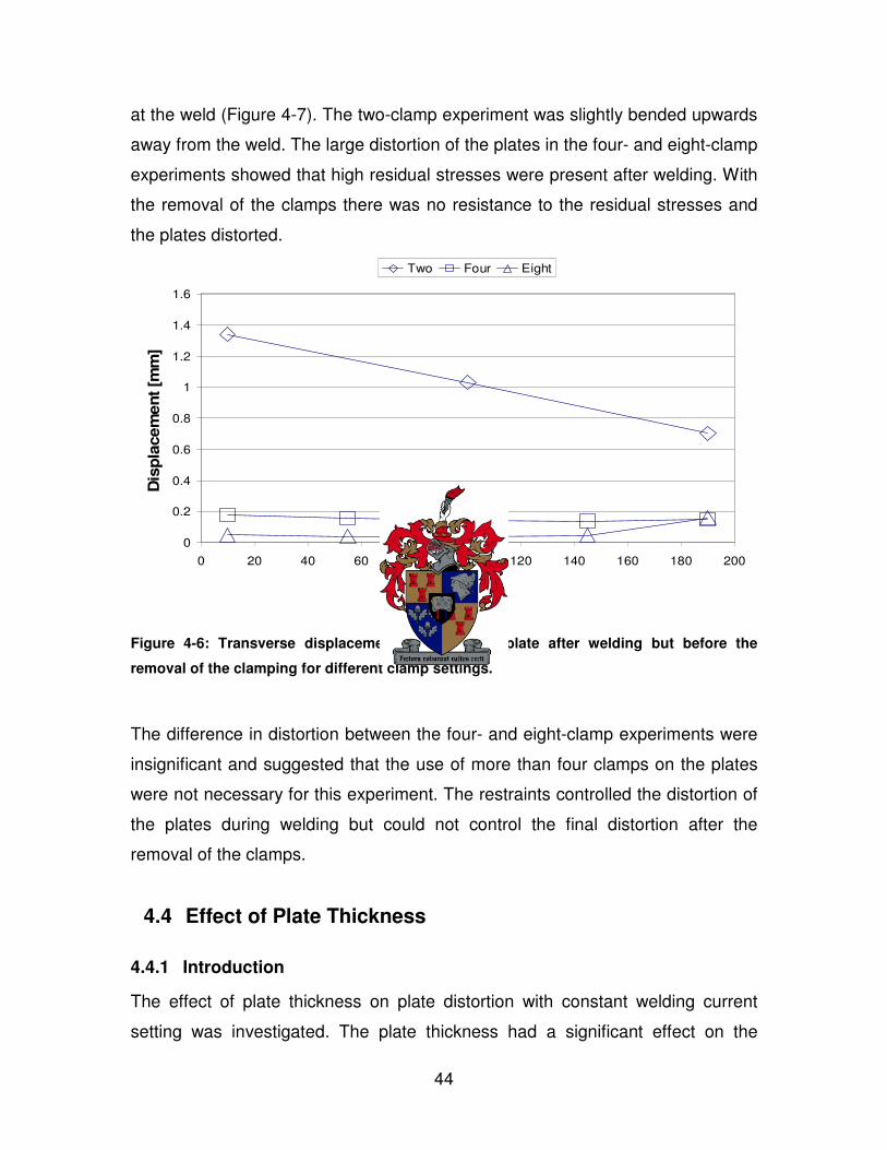
44
at the weld (Figure 4-7). The two-clamp experiment was slightly bended upwards
away from the weld. The large distortion of the plates in the four- and eight-clamp
experiments showed that high residual stresses were present after welding. With
the removal of the clamps there was no resistance to the residual stresses and
the plates distorted.
0
0.2
0.4
0.6
0.8
1
1.2
1.4
1.6
0 20 40 60 80 100 120 140 160 180 200
Y [mm]
Dis
pla
cem
ent [m
m]
Two Four Eight
Figure 4-6: Transverse displacement in middle of plate after welding but before the
removal of the clamping for different clamp settings.
The difference in distortion between the four- and eight-clamp experiments were
insignificant and suggested that the use of more than four clamps on the plates
were not necessary for this experiment. The restraints controlled the distortion of
the plates during welding but could not control the final distortion after the
removal of the clamps.
4.4 Effect of Plate Thickness
4.4.1 Introduction
The effect of plate thickness on plate distortion with constant welding current
setting was investigated. The plate thickness had a significant effect on the

45
magnitude of plate distortion with the thinner plates experiencing the largest
distortions. This phenomenon can be explained in terms of the thinner plates
being lighter in mass and less in bending stiffness. This means that thinner plates
are more likely to welding distortion than thicker plates.
3
3.5
4
4.5
5
5.5
6
6.5
0 20 40 60 80 100 120 140 160 180 200
Y [mm]
Dis
pla
cem
ent [m
m]
Two Four Eight
Figure 4-7: Transverse displacement in the middle of the pate after removal of clamps.
Figure 4-8: Order of the removal of clamps.

46
The experiment was done on 2, 3 and 4 mm thick mild steel plates. Four clamps
in total, two on each plate, were used and a welding current of 90 A was used.
The clamps in every experiment were removed in a specified order ending with
the reference clamp. The order of removal of the clamps is shown in Figure 4-8.
This procedure ensured repeatable experimental results.
4.4.2 Results
To avoid burning through of the plates, the welder increased the welding speed
with the thinner plates. The change in welding speed did not have an effect on
the current or voltage of the welding, thus the power output remained constant at
around 2157 W (Table 4-2). The average welding current and voltage for the
experiments were 85.76 A and 25.25 V respectively, giving an error of 4.7% for a
current setting of 90 A. The assumption of 25 V for the voltage of the process
proved to be an accurate assumption for the 90 A setting on the machine.
The average welding speed for the 2 mm thick plate was 5.53 mm/s, which was
significantly faster than the 3.71 and 3.26 mm/s for the 3 and 4 mm thick plates
respectively. The overall welding length for the 4 mm plate was shorter due to the
fact that the electrode was consumed before the end of the plates.
Table 4-2: Average welding process parameters for different plate thickness.
Power
[W]
Current
[A]
Voltage
[V]
Time of weld
[s]
Weld Length
[mm]
Weld Speed
[mm/s]
2 mm 2161.33 86.06 25.20 36.25 199.00 5.53
3 mm 2154.36 83.99 25.75 54.02 200.00 3.71
4 mm 2156.68 87.23 24.80 53.92 175.67 3.26
Ave 2157.46 85.76 25.25 48.06 191.56 4.17

47
Table 4-3: Energy input parameters for different plate thickness.
Energy [J] P/v [J/mm]
2 mm 78348.21 390.84
3 mm 116378.53 580.69
4 mm 116288.19 661.56
Ave 103671.64 544.36
The energy input determined the heat input into the weldment. Table 4-3 shows
the total energy in Joule and energy per unit length in Joule per millimetre. The
total energy was calculated from the product of the power and time of welding
(Equation 4-1). The total energy for the 3 and 4 mm (116 kJ) plates were almost
the same while significantly less energy was used for the 2 mm thick plate
(78 kJ). The welding processes could not be compared on grounds of total
energy input because the length of the welds was not the same for all of the
experiments.
VIP = Equation 4-1
The energy per unit length gave a better indication of the difference in heat input
of the welding process and was calculated with the power divided by the welding
speed (Equation 4-2). It was assumed that the power remained constant for the
experiments and the welding speed were the only variable. An increase in
welding speed resulted in less energy per unit length. This meant that the 2 mm
thick plate had 41% less heat input than the 4mm thick plates (Table 4-3. Even
with less heat input the 2 mm plate distorted more than the thicker plates.
v
PEl =
Equation 4-2
Wells developed approximations for the relationship between heat input and the
product of the welding speed and weld width divided by the thermal diffusivity of

48
the metal (cited by Lancaster, 1965). Equation 4-3 shows this relationship for the
2D case where the weldment had fused through the thickness of the plate. It was
assumed there was no temperature gradient through the thickness of the plate.
+=
α45
18
vdkT
h
qm Equation 4-3
Equation 4-3 shows that for a given plate thickness, h, a minimum rate of heat
input is required in order to make a full penetration weld. This was considered the
optimum welding heat input requirement for a given plate thickness and base
material. Figure 4-9 shows the theoretical heat input as determined with Equation
4-3 compared with the measured heat input in the experiments. From Figure 4-9
it can be seen that the heat input for the 3 mm thick plate was at the optimum
value while the 2 mm plate lay above the theoretical value and the 4 mm plate
below the line. This meant that the welder used the optimal current settings and
welding speed for the 3 mm thick plate. The heat input used for the 2 mm thick
plate were above the optimum values and explains the almost burning through of
the plates during welding. The graph in Figure 4-9 shows that more heat could be
put into the 4 mm plate to obtain a weld through the thickness of the plate.
The comparison of Equation 4-3 with the measured values proved that the
human welder operated at optimum conditions and had the ability to adjust the
welding process for different welding situations. The heat input values for the
standard 3 mm thick plate were repeatable. The spreading of the heat input for
the 2 mm thick plate could be attributed to difficulty controlling the welding at high
speeds.
The distortions of the welded plates increased with a decrease in plate thickness.
The displacement trends for the 2 and 3 mm plates were the same while the
4 mm plates showed little distortion. The maximum displacement recorded for the
2, 3 and 4 mm plates were 7.52, 5.18 and 1.27 mm respectively. All three the
maximum displacements were recorded at the coordinates X = 190 mm and Y =

49
190 mm, the point closest to where the weld was finished (see Figure 4-10). The
clamps closest to these maximum points were released first after welding. The 2
and 3 mm plates distorted much more than the 4 mm plate, even though more
energy was put into the 4 mm plate.
100000
200000
300000
400000
500000
600000
700000
800000
0 0.002 0.004 0.006 0.008
v [m/s]
q/w
[W
/m]
Theory 2D h = 2mm h = 3mm h = 4mm
Figure 4-9: Welding speed vs. heat input per unit thickness for welding of plates with
different thickness.
The location of the maximum deflection at the edge where the weld finished
could be due to the lack of heat dissipation near the edge of the plate. During
welding the heat flow away from the weld occurred through conduction of the
steel. Near the edge of the plate the amount of material in front of the welding
was less, thus a decreasing heat sink effect. This caused the plates to be the
hottest at the end of the weld and in turn creating larger distortions.
The plate deflection on a line perpendicular (transverse) to the weld in the middle
of the plate is shown in Figure 4-11. The 2 mm thick plate had the greatest
deflection near the weldment (Y = 190 mm) while the 4 mm plate had relatively

50
no displacement. The 3 mm plate experienced moderate deflection compared to
the 2 mm plate, with a maximum displacement of 3.15 mm at the weldment.
Figure 4-10: Point of maximum deflection for welded plates in the experiments.
The deflection of the plates on a line parallel (longitudinal) to the weldment at a
distance of 10 mm from the weld on the side opposite to the reference clamp are
shown in Figure 4-12. The deflection of the 2 mm plate showed the familiar
longitudinal bending-up of the plates at the edges. This phenomenon occurred
due to heat being dissipated at a slower rate at the edges than in the middle of
the plate. This effect was observed for the 3 and 4 mm thick plates but to a lesser
degree.

51
0.00
1.00
2.00
3.00
4.00
5.00
6.00
7.00
8.00
0 50 100 150 200
Y [mm]
Dis
pla
cem
ent [m
m]
2mm 3mm 4mm
Figure 4-11: Transverse displacement for different thickness after removal of clamps.
The plates deflected the most after the last clamp (reference clamp) had been
removed from the plates. During the removal of the other three clamps the plates
showed minimal distortion. This plate deflection occurred due to the welding
induced residual stress that caused the deflection of the plates when the
restrictive forces of the clamps were removed.
The displacements of the plates with only the reference clamp on the plates at
the locations as shown in Figure 4-11 and Figure 4-12 are shown in Figure 4-13
and Figure 4-14 respectively. The 2 mm thick plate showed large deflection with
only the reference clamp on the plates, while the 3 and 4 mm plates experienced
little deflection. In Figure 4-14 the plates deflected the most at the edge of the
plate where the first clamp was removed and the deflection decreasing up to the
location of the reference clamp (Y = 10 mm).

52
0.00
1.00
2.00
3.00
4.00
5.00
6.00
7.00
8.00
0 50 100 150 200
Y [mm]
Dis
pla
cem
ent [m
m]
2mm 3mm 4mm
Figure 4-12: Final longitudinal displacement for different plate thickness, after removal of
all clamping.
The results from the experiment had shown that the plate thickness had a greater
influence on the plate distortion than the energy input per unit length. The 2 and
3 mm thick plates had full penetration welds, while the 4 mm thick plate did not
have a full penetration depth. From Equation 4-3 it was seen that the 2 and 3 mm
plates were welded at optimal energy input and the 4 mm thick plate below the
optimal energy input value.
The excessive distortion of the 2 mm plate could be attributed to two factors.
Firstly, the thinner plate had less bending stiffness and less weight to resist the
deflection of the plates and secondly the 2 mm thick plates experienced the
maximum heat input, without burning through, causing excessive distortion.

53
-0.8
-0.6
-0.4
-0.2
0
0.2
0.4
0.6
0.8
1
1.2
0 50 100 150 200
Y [mm]
Dis
pla
cem
ent [m
m]
2 mm 3 mm 4 mm
Figure 4-13: Transverse displacement for different plate thickness with only reference
clamp on plates.
-0.4
-0.2
0
0.2
0.4
0.6
0.8
1
1.2
1.4
0 50 100 150 200
Y [mm]
Dis
pla
cem
ent [m
m]
2 mm 3 mm 4 mm
Figure 4-14: Displacement of plates with reference clamp: longitudinal displacement.

54
4.5 Effect of Current Setting
4.5.1 Introduction
The effect of plate displacement with different electric current settings was
investigated on the 3 mm mild steel plates. Welding current settings of 70, 90
and 110 A were investigated. The experiments were compared on final plate
displacement, power input and energy per unit length.
The increase of welding current means an increase in power and heat input. The
change in welding power was investigated to determine the influence on plate
distortion. With an increase of heat input, larger deflections were expected if all
other welding parameters remained the same. Since the welder was free to
change welding speed with different current settings, the heat input per unit
length did not increase with the current, as was expected.
4.5.2 Results
The amount of heat input gave an indication of the expected distortion: more heat
input meant more plate distortion. The heat input is increased by increasing the
welding current, but the welder succeeded in keeping the energy input constant
by changing the welding speed. The average calculated energy per unit length
for nine experiments was 556 J/mm (Table 4-5). The average measured current
for the 70, 90 and 110 A settings were 70.66, 83.99 and 104.19 A (Table 4-4).
The lower measured welding current for the 110 A setting could have been
caused by the rapid increase in temperature of the welding electrode since the
specified current for the electrode used was 69 – 95 A. An increase in electrode
temperature caused an increase in electrical resistance and a drop in current.

55
Table 4-4: Average welding process parameters for different current settings.
Power Current Voltage Time Length Speed
70 A 1716.89 70.66 24.39 64.54 199 3.10
90 A 2154.36 83.99 25.75 54.02 200 3.71
110 A 3008.62 104.19 28.76 35.62 200 5.64
Ave 2293.29 86.28 26.30 51.39 199.67 4.15
Table 4-5: Average energy input parameters for different current settings.
Energy [J] P/v [J/mm]
70 A 110808.08 553.84
90 A 116378.53 580.69
110 A 107167.04 533.44
Ave 111451.22 555.99
The 110 A current setting gave the least plate deflections and the 90 A setting
the highest. In the case of the 70 A setting low power was available from the
machine and the welder had to decrease the welding speed to obtain a sufficient
bond. With the high power input from the 110 A setting the welder increased the
welding speed to prevent burning through of the material. This adjustment of the
welding speed by the welder had resulted in the 110 A setting to have the lowest
heat input per unit length and the 90 A the highest (Table 4-5).
The maximum plate deflections measured for the 70, 90 and 110 A setting was
4.01, 4.74 and 2.49 mm respectively. Figure 4-15 shows the transverse
displacement at a distance 190 mm from the start of the weld. The 110 A setting
had by far the least deflection while the 70 and 90 A setting had similar
displacement results.
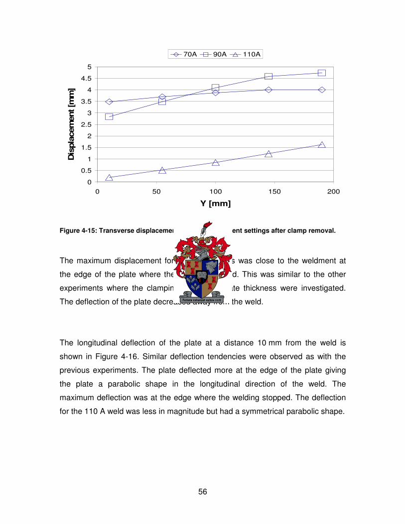
56
0
0.5
1
1.5
2
2.5
3
3.5
4
4.5
5
0 50 100 150 200
Y [mm]
Dis
pla
cem
ent [m
m]
70A 90A 110A
Figure 4-15: Transverse displacement for different current settings after clamp removal.
The maximum displacement for the experiments was close to the weldment at
the edge of the plate where the welding stopped. This was similar to the other
experiments where the clamping effect and plate thickness were investigated.
The deflection of the plate decreased away from the weld.
The longitudinal deflection of the plate at a distance 10 mm from the weld is
shown in Figure 4-16. Similar deflection tendencies were observed as with the
previous experiments. The plate deflected more at the edge of the plate giving
the plate a parabolic shape in the longitudinal direction of the weld. The
maximum deflection was at the edge where the welding stopped. The deflection
for the 110 A weld was less in magnitude but had a symmetrical parabolic shape.

57
1.00
1.50
2.00
2.50
3.00
3.50
4.00
4.50
5.00
0 50 100 150 200
X [mm]
Dis
pla
cem
ent [m
m]
70A 90A 110A
Figure 4-16: Final displacement for different current settings, longitudinal displacement.
The smaller deflections observed for the 110 A current setting could be attributed
to lower heat input per unit length caused by higher welding speeds. Full
penetration welding was not achieved along the whole length of the plate for the
110 A setting. This could have resulted in smaller contraction forces than for the
90 A settings where full penetration was achieved. The slow welding speed for
the 70 A setting resulted in better penetration and heat distribution than the
110 A setting, even though the welding machine were operating at less power
(Table 4-4).
The heat input was at its highest for the 90 A setting because the welding
electrode could operate normally and the plate thickness was sufficient to absorb
the heat input without burning through. The plate deflection was the most for the
90 A setting but the weld strength was the best due to better edge penetration.

58
4.6 Temperature Measurement
4.6.1 Introduction
The first step in creating a scientific base for the design and analysis of welds is
to accurately compute the transient temperature fields. The high temperatures
developed by the localised heat source cause significant metallurgical changes in
low carbon steels. The measured temperatures were used to determine the
temperature distribution in the plates for the experimental set up and to verify the
FEM temperature results with the experiments. The experiment was repeated
three times with the same settings and conditions to investigate the repeatability
of the results.
The thermocouple is the most common method used to measure temperature.
This is due to the fact that it is cheap, interchangeable and can measure a wide
range of temperatures. A thermocouple consists of two wires of different metals
that are joined at one end. A change in the temperature at the connection of the
two wires will induce a change in the electromotive force (EMF) between the
open ends. As the temperature changes, the EMF will change. Often the
thermocouple wires are located inside a metal or ceramic shield that protects it.
The most commonly used thermocouple type for measuring high temperatures is
the type K. It has one wire of nickel-chromium and one of nickel-aluminium.
Nine K – type thermocouples with a diameter of 0.5 mm wire, spot-welded onto
the plates at locations shown in Figure 4-17. The objective of the layout of the
thermocouples was to obtain temperature trends in the planes transverse and
longitudinal to the weld line. The temperature data was recorded with a
HP 34970A data acquisition unit at one-second intervals for every thermocouple.
The thermocouples were placed in rows transverse to the weldment at distances
20, 50 and 150 mm from the weldment and in longitudinal direction at distances
30, 50 and 100 mm from the start of the weld (Figure 4-17). The first row of

59
thermocouples (X = 30) was close to the welding jig/plate interface. The
temperature results from these thermocouples were compared with the other
temperatures at the other thermocouples to determine the heat sink effect of the
jig.
Figure 4-17: Thermocouple locations on welded plates.
The spot welding of thermocouples to a plate proved to be a sufficient bond, but
there was a problem with the wires that broke off easily at the spot weld. This
was solved by attaching the wires to the plate for a distance with an adhesive
bond to prevent a direct pull on the wires at the spot weld.
TIG welding was used to fuse the thermocouple wires in an inert gas
environment. The wires were fused into a small lump which was then spot
welded to the plate (Figure 4-18). Care was taken to ensure that the wires did not
make contact outside the spot weld. The thermocouples were located
underneath the plate, at the opposite face of the weld bead to minimize radiation
disturbance effects from the arc and the environment. It was assumed that the
temperature difference through the thickness of the plate was negligible.

60
Figure 4-18: Thermocouple spot-welded to mild steel plate.
4.6.2 Results
A thermocouple measures the temperature at the first contact between the two
wires (Dally, Riley & McConnell, 1993). The contact point of the thermocouple
wires was inside the spot weld and the distance of the spot weld to the centre of
the weld was measured. High spatial temperature gradients existed near the
weld and it was therefore important that the placement of the thermocouples had
to be accurate and repeatable for the three experiments.
The measured distances from the centre of the weld to the contact point of the
thermocouple is shown in Table 4-6. The average error in distance of the
measuring point relative to the specified point for the thermocouple was 1.6 mm.
The average error for the thermocouples 20 mm from the weld was 1.3 mm. This
was an acceptable tolerance level and it was assumed that the thermocouples
measured temperatures at the same distances from the weld in the three
experiments. The true distance of the thermocouples were used in the modelling.

61
Table 4-6: Distance of thermocouple measuring point to centre of weld.
Distance of thermocouple contact from centre of weld
Point 1 2 3 4 5 6 7 8 9
Specified
Distance 20 50 150 20 50 150 20 50 150
Experiment
#1 18 48 148.5 18 47 148 17 46 148
#2 21 53 149 21 51 152 20 50 151
#3 22 52 152 20 51 153 21 49 151
Average 20.3 51.0 149.8 19.7 49.7 151.0 19.3 48.3 150.0
The highest temperature variation was measured at the thermocouples located at
X = 100 mm, the centreline of the plate perpendicular to the weld. The
thermocouples close to the jig/plate interface (X = 30 and 50 mm) recorded lower
temperatures. The welding rig acted as a heat sink, which lead to faster cooling
of the plate near the welding rig. A difference of 41.4 °C was measured for the
maximum temperatures at the thermocouples 20 mm from the weld at 30 and
100 mm from the initial weld position (Figure 4-19). At 50 mm from the weldment
the difference of ΔT = 54 °C was bigger than at 20 mm from the weld.
The maximum temperatures measured at the thermocouples compared
significantly well with the analytical solution proposed by Rosenthal. The
temperatures from the analytical solution were higher because convective and
radiation heat losses are not taken into consideration and constant material
properties were assumed.
The temperatures were the highest at the centre of the plate, furthest away from
the jig. In the second experiment the temperatures close to the jig,
X = 30 and 50 mm, were higher than for the first and third experiment. The
clamps were not fastened as tight in the other experiments and the contact heat

62
transfer coefficient between the plate and jig was thus lower, resulting in higher
temperatures. The clamping force was not measured and was initially not
considered important in the temperature measurement experiment. From the
experiments it was clear that the contact pressure due to clamping had a
significant effect on the temperature distribution.
0.00
50.00
100.00
150.00
200.00
250.00
300.00
350.00
0 50 100 150 200 250 300
Time [s]
Tem
pera
ture
[°C
]
X = 30 mm X = 50 mm X = 100 mm
Figure 4-19: Maximum temperatures of thermocouples at distance 20 mm from weld.
The average percentage in maximum temperature difference between the
thermocouples in the three experiments was 3.04%. Little difference in results
could be seen for the temperature distribution graphs at a distance 20 mm from
the weld in the middle of the plate (Figure 4-21). The repeatability of the
temperature measurements for the three experiments was excellent and could be
used for verification with FEM results.

63
0
50
100
150
200
250
300
350
400
0 20 40 60 80 100 120 140 160
Distance [mm]
Tem
pera
ture
[°C
]
Row 1 Row 2 Row 3 Analytical
Figure 4-20: Comparison of maximum temperatures in transverse line with analytical
solution.
0.00
50.00
100.00
150.00
200.00
250.00
300.00
350.00
0 50 100 150 200 250 300
Tim e [s]
Tem
pera
ture
[°C
]
F1 F2 F3
Figure 4-21: Temperature distribution at distance 20 mm from weld in centre of plate for
three different experiments.

64
4.7 Conclusion on Experiments
Experiments were carried out to investigate the effect of changes in welding
parameters on the distortion of the welded plates. The parameters investigated
were;
• the number of restraints on the clamps,
• the plate thickness and
• the welding current.
Low, medium and high values were given to these parameters. The median
values were taken from a standard experiment that was created and values lower
and higher were appointed for the other experiments.
The effect of restraints was investigated for two, four and eight clamps on the
plates. The lack of restraint in the two-clamp experiment caused the plates to be
misaligned. This caused excessive distortion in one plate during welding. The
plates did not distort significantly more after the removal of the clamps.
In the four and eight clamp experiments no significant displacements was
measured after welding with all the clamps still on the plates and distorted after
the removal of the clamps. This indicated that residual stresses were building up
in the plates and caused the plates to distort after the removal of the restraining
forces.
The plate thickness had significant effect on the distortion of the plates. The
maximum displacement for the 2, 3 and 4 mm thick plates were 7.52, 5.18 and
1.27 mm respectively. The welder avoided burning through of the material with
the 2 mm thick plates by increasing the welding speed, thus decreasing the heat
input per unit length. The welding speed used for different plate thickness
coincided with theoretical equations.
An increase in welding current increases the power input of the welding process.
The power input of the welding process did not affect the heat input per unit

65
length. The welder maintained a constant heat input per unit length by increasing
the welding speed with an increase in welding current. The maximum
displacements for the 70, 90 and 110 A current settings were 4.01, 4.74 and 2.49
mm respectively.
66
5 MODELLING OF WELDING EXPERIMENTS
5.1 Introduction
Finite element analysis (FEA) has been used by many authors to predict welding
distortions and temperature distributions in different types of joints and materials
(Deo, et al., 2002, Michelaris, et al., 1996, Moshaiov, et al., 1990). Prediction is
difficult due to the complex variations of temperature, thermal contraction and
expansion and variation of material properties with temperature. Furthermore,
modelling of the weld process must account for the specialized effects of the
moving weld arc and material deposit.
Finite element (FE) models of the welding experiments were carried out to verify
the validity of the numerical results. The numerical and experimental results were
verified on temperature and plate displacement results. The finite element
method was used to obtain results that were not measured in the experiments
like stresses and strains, giving insight into the welding process that cannot be
seen in the workshop.
The main modelling parameters investigated were the material properties,
element mesh density, weld modelling tool options and analysis options. In the
analysis options the time step size, convergence tolerances and job options were
significant in the analysis. The application of the modelling parameters is
discussed in this chapter. The use of thermal analysis, structural analysis with
temperature history definition and coupled thermo-mechanical analysis were
performed in this thesis. Modelling techniques were investigated to obtain an
effective finite element model for welding simulation.
67
5.2 Weld Modelling in MSC.Marc
The FEM solver MSC.Marc with the pre- and postprocessors MSC.Patran and
MSC.Mentat were used in this research. MSC.Marc is a non-linear commercial
FEM software package that has the capabilities to perform welding simulations.
Special model definition options for the simulation of welding are available in
MSC.Marc/Mentat.
Welding is a thermal process with specialized boundary conditions. These
boundary conditions are specified through the definition of the weld flux in
conjunction with the specification of the weld path and filler metal options. The
pre-defined moving heat source tools include, but not limited to, the Goldak
double ellipsoidal heat source model. Filler metal deposition is defined via
element activation/de-activation.
Additional items to facilitate welding analysis in MSC.Marc are time stepping,
convergence checking and adaptive meshing. Adaptive time stepping was used
in the weld models where the increment time was estimated through the
allowable temperature change per increment. Convergence tolerances were
relaxed to decrease modelling time but without threatening the accuracy of the
results. Non-linear temperature dependent material properties and latent heat
effects were specified.
5.3 Weld Model Preparation
5.3.1 Geometry and Element Meshing
As with any finite element analysis, the first step was the modelling of the
geometry and element mesh. This was done in MSC.Patran due to its user-
friendly and powerful geometry and meshing tools. An input file was created in
MSC.Patran and imported into MSC.Mentat. MSC.Patran was not fully

68
compatible with all the capabilities of MSC.Marc while MSC.Mentat is the original
pre- and postprocessor for MSC.Marc.
Four node shell elements with the option of quadratic temperature distribution
through the thickness of the elements were used. The elements had the option of
three integration points through the thickness of the element, which was
considered to give an accurate estimation of the temperature distribution through
the plate thickness. These elements were suitable for thermal and coupled
thermal-structural analysis.
As a rule, elements behave best when it were of a compact regular shape (Cook,
R.D., 1995), thus the elements were kept rectangular throughout the model. The
element aspect ratio was kept below 5:1 in the weld region and increased
towards the far edge of the plate to an aspect ratio of 10:1.
The size of the elements in the welding region was determined through
guidelines that Goldak had proposed for accurate representation of the heat
source model. The Gaussian ellipsoidal model required approximately four
quadratic elements along each axis to capture the inflection of the Gaussian
distribution (Goldak, et al., 1986). An element size of 2 x 1 mm was used in the
weld zone which satisfied the guidelines proposed by Goldak. This captured
more accurate temperature results without an analysis time penalty. The
geometrical heat source values for the standard experiment were 5, 3, 2.5 and
10 mm for the width, depth, forward length and backward length respectively
resulting in 2.5 and 6.25 elements in the width and length of the heat source.
5.3.2 Material Properties
The metal most widely used in welded fabrication is carbon steel containing up to
about 0.3% carbon (mild steel). This material undergoes only minor hardening in
the heat-affected zone of fusion welds and normally is welded without any pre- or

69
post welding heat treatment. Mild steel is easily available, cheap and can be
welded by most of the welding processes. This steel was chosen for these
experiments due to its relatively problematic free weldability.
The material properties were discussed in Chapter 3.5. The temperature
dependent material properties specified in the model were conductivity, specific
heat, elastic modulus, yield strength and thermal expansion coefficient. Latent
heat of solidification can be specified in the material specification options list.
Various authors specified the latent heat of fusion for low carbon steel as
260 kJ/kg (Goldak, et al., 1986). The mass density remained constant at all times
with a value of 7850 kg/m³. The melting range for mild steel was taken as 1432 –
1526 °C.
Non-linear temperature dependent material properties were specified in the
model. The models were improved systematically from constant properties to
temperature dependent properties, improved conduction for weld pool convection
and latent heat effects. The use of temperature dependent material properties in
the structural analysis required smaller time steps, due to the low Young’s
modulus at high temperature.
5.3.3 Boundary Conditions
The loads and boundary conditions in a model are everything that operates in the
immediate environment that is not explicitly modelled. The loads and constraints
specified in the thesis were divided into two groups: thermal and structural
boundary conditions. The thermal boundary conditions were the heat source,
initial temperature, thermal contact, weld filler initial temperature and
convection/radiation heat losses. The structural conditions were the restraints put
on the plates by the welding jig and clamps and the restrictions in the plane of
symmetry. In the uncoupled structural analysis the thermal history was applied as
a state variable.

70
5.3.3.1 Thermal Boundary Conditions
The most important thermal boundary condition specified in the welding analysis
was the applied heat source. The double ellipsoidal heat flux volume was
discussed in Chapter 3.1.5 and will not be explained in detail in this section. No
guide for the sizing of the heat source model existed and values were chosen
until the correct molten zone size was produced. It was found that to get a correct
weld pool size, smaller dimensions had to be used. This is due primarily to the
interaction between the heat source power, which is Gaussian along the
longitudinal weld arc axis, and the volume specified by the double ellipsoid
dimensions (Francis, 2002).
The heat source parameters were determined by measuring the rippling effects
of the weld beads. In the absence of sufficient measurements the distance in
front of the heat source was taken equal to one-half the bead width and the
distance behind the heat source equal to twice the width (Goldak, et al., 1984).
The heat source parameters used in the modelling for the different experiments
are shown in Table 5-1. The welding speeds and power input were the average
calculated values from the experiments. The value of the arc efficiency was taken
as ηarc = 0.5 from the literature (Groover, 1999). Small changes in the arc
efficiency had a negligible effect on the temperature distribution since the filler
metal was specified with an initial melting point temperature of 1480 °C.
Table 5-1: Experimentally determined heat source parameters.
Width Depth Front length Back length Speed Power arc efficiency
Two 7 3 3.5 14 3.67 2174 0.7
Four 7 3 3.5 14 3.71 2155.4 0.7
Eight 7 3 3.5 14 3.31 2264 0.7
2 mm 6 2 3 12 5.53 2161.3 0.7
3 mm 7 3 3.5 14 3.71 2155.4 0.7
4 mm 8 4 4 16 3.26 2156.7 0.7
70 A 7 3 3 14 3.1 1716.89 0.7
90 A 7 3 3.5 14 3.71 2154.36 0.7
110 A 6 3 3 12 5.64 3008.62 0.65
Clamps
Plate
Thickness
Current

71
The theory on the combined convection and radiation heat transfer coefficient
was explained in Chapter 3.3.7 and Appendix A. This data was specified via a
face film boundary condition and applied to all the free surfaces of the plate.
The heat sinking effect of the welding jig had a significant effect in the
temperature results. In the thermal analysis heat transfer coefficients were
specified between the plate and welding jig. The contact heat transfer coefficient
was taken as 7500 W/m².°C and the near contact heat transfer coefficient as
1000 W/m².°C. The ambient temperature and initial temperature was taken as
25 °C.
5.3.3.2 Structural Boundary Conditions
The major boundary conditions specified for the structural analysis were the
welding jig contact and the clamps. The contact area of the welding jig and
clamps were modelled as rigid bodies. The jig was kept rigid for the whole
duration of the analysis, while the clamps were removed just before the end of
the model. Symmetrical boundaries conditions were applied at the centre of the
weld line to prevent movement perpendicular through the weld centreline (X -
translation fixed) and movement along (longitudinal and up-/downwards) the weld
centreline (Y - and Z - translation fixed).
In the uncoupled structural analysis the thermal history was specified as a state
variable. The state variable used the thermal history obtained in the thermal
analysis and mapped in on every node for the structural analysis.
5.3.4 Element Activation/De-Activation
MSC.Marc uses the element activation/de-activation option for the dynamic
creation of filler elements and the generation of associated boundary conditions.

72
Two methods are supported for the creation of the filler elements: the quiet
element method and the deactivated element method.
In the quiet element method the filler elements are initially used with scaled down
material properties with a default factor of 10-5. When the filler elements are
physically created by the moving heat source, all stresses and strains in the
elements are reset to zero and used with regular material properties. The
drawback of the quiet element method is that it is prone to ill conditioning due to
large discrepancy in the material stiffness.
In the deactivated element method, filler elements are initially deactivated in the
analysis and are not shown on the post file. The elements are physically created
when all the nodes are inside the “box” of the heat source model. This method
does not suffer from ill conditioning problems but can cause distorted filler
elements when used in large deformation welding analysis. The deactivated filler
elements were used in the coupled analysis and the quiet element method was
used in the uncoupled analysis.
5.3.5 Coupled and Uncoupled Analysis
The uncoupled analysis approach was used instead of the coupled thermo-
structural analysis. The coupled analysis proved to be resource intensive and
time consuming. By separating the thermal and structural analysis, better control
and monitoring of the analysis was achieved. It was assumed that the
deformations in the structural analysis had no influence on the temperature
distribution. The thermal analysis of the welding process was performed with
thermal contact of the welding jig taken into consideration. The jig and the plate
were modelled as rigid bodies with heat transfer capabilities.
The temperature results from the thermal analysis were applied as a boundary
condition in the structural analysis. All analyses were done for 600 s at which

73
time the plate temperature had cooled down close to ambient temperature. After
600 s the clamps on the plates were removed, to simulate the plate deformation
during the removal of the clamps.
5.4 Numerical Results
The modelling results did not compare accurately with the experimental results,
but similar trends were found in the FEM results. The displacement results were
compared directly with the experimental results, while each model was compared
on grounds of temperature distribution and vertical displacement.
5.4.1 Thermal Results
5.4.1.1 Effect of Different Plate Thickness
Even though the input power for the welding of different plate thickness was
constant, the time of weld differed greatly. This caused different heat input into
the steel plates. From the FEM results it was clear that the different welding
speeds affected the maximum temperatures and cooling of the plates.
With the slower welding speeds for the 3 and 4 mm thick plates, more heat was
put into the plates. This meant higher peak temperatures, which had several of
affects on the welded structure. This included a larger heat affected zone (HAZ)
and longer time of cooling to room temperature. The thicker plates have more
material and thus more heat storage capacity, thus keeping the heat longer.
Steel plates of different thickness welded at the same welding parameters had
difference in temperature distribution and cooling time of the plates. The thicker
plates could absorb more heat for a sufficient bond, thus causing higher peak
temperatures and longer cooling of the plates. After 600 s, there was a significant
difference between the plate temperatures for different plate thickness (Figure
5-1). This indicated that with an increase in plate thickness there is an increase in
production “recycling time”, due to slower plate cooling.

74
20.00
40.00
60.00
80.00
100.00
120.00
140.00
0.00 100.00 200.00 300.00 400.00 500.00 600.00
Time [s]
Tem
pera
ture
[°C
]
2mm 3mm 4mm
Figure 5-1: Temperature distribution for different thickness, 50 mm from weld.
5.4.1.2 Effect of Different Current Settings
The FEM results for different welding current settings have shown that the
highest temperature distribution was in the 70 A welding process. The slower
welding speed for the 70 A welding resulted in an increase in energy per unit
length (see Equation 4-2). The 110 A welding current setting gave the lowest
temperature distribution.
Although the 70 A current setting gave the highest temperatures, it did not give
the overall maximum plate displacement in the experiments. The plates welded
with the 90 A setting gave the largest displacement while the 110 A the least.
The displacement for the 70 A setting was in between. The structural results will
be discussed in Section 5.4.2.
Unlike the temperature results for different plate thickness, the cooling of the
plates were the same, which indicated that the plate thickness is an important

75
factor in the cooling of the plates. The cooling of the plates were almost the same
because in all three experiments the plates had the same stored heat capacity.
Steel plates of the same thickness welded at different welding current settings
have the same cooling time. The only difference was in the time of the weld itself:
the higher the current, the faster the welding speed. The difference in
temperature of the steel plates after 600 s did not differ greatly, thus concluding
that a difference in welding current do not have a significant effect on the
“recycling time” of a welded structure, except for the time of the weld itself.
5.4.2 Structural Results
The thermal results were applied as boundary conditions in the structural
analysis. Shell elements with quadratic temperature distribution between the
nodes were used in the structural analysis. The assumptions discussed in the
Section 3.2.4 were applied structural analysis.
It was assumed that the temperature distribution in the welded plates was
symmetrical and only one plate was modelled. Only the displacement results
were verified with experimental results, while the stress results gave insight to
the residual stress distribution in the welded plates. The displacement results
were investigated by using the same 25-point measuring grid used in the
experiments. The displacements were compared on lines parallel (longitudinal)
and perpendicular (transverse) to the weldment.
The welding process was modelled over a period of 600 seconds with the clamps
attached to the plates. From 600 to 610 seconds the contact surfaces of the
clamps were gradually released to simulate the removal of the clamps. The most
distortion of the plates occurred during the removal of the clamps.

76
Assumptions made in experiments and models regarding the environmental
effects could have attributed to results that did not validate accurately with the
experimental results. The effects of assumptions made in the modelling were not
investigated in this study, since it fell outside the scope of this thesis.
5.4.2.1 Effect of Different Plate Thickness
The displacement results of the welding analysis of 2, 3 and 4 mm thick mild
steel plates gave good comparison with the displacement tendencies observed in
the welding experiments but not as accurate in the magnitude of the plate
displacement. The experimental results were only used as a base of comparison
and were taken as absolute.
With the use of shell elements, the plate thickness could be changed without
changing the model. This did imply that the contact tolerances specified in the
models had to be adjusted accordingly with the change in plate thickness. The
welding heat input parameters were also specified with values obtained from the
experiments.
The thinner plates underwent the most distortion as was observed in the
experiments. The 4 mm plate showed the least distortion (0.06 mm) and the
2 mm thick plate showed overall the most deflection (1.96 mm), although the
maximum vertical displacement was found in the 3 mm thick plate model
(2.61 mm). Figure 5-2 shows the plate displacement perpendicular to the
weldment in the middle of the plate (X = 100 mm). In the graph the centre of the
weldment is at Y = 200 mm.
The maximum recorded vertical displacement (Z-direction) for the 3 mm FEM
model could be attributed to the contact tolerances in the model. With the
releasing of the clamps in the model, the shell elements can still “cling” onto the
contact surfaces moving away, before the deformable body and contact surface
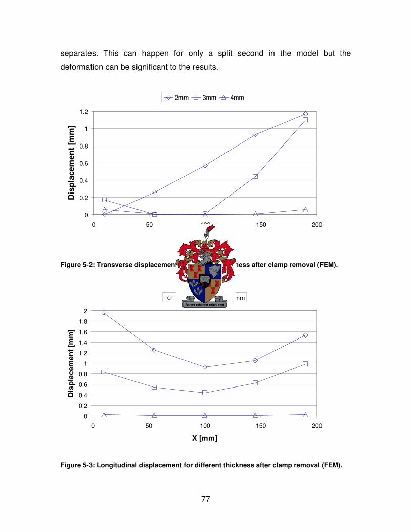
77
separates. This can happen for only a split second in the model but the
deformation can be significant to the results.
0
0.2
0.4
0.6
0.8
1
1.2
0 50 100 150 200
Y [mm]
Dis
pla
cem
en
t [m
m]
2mm 3mm 4mm
Figure 5-2: Transverse displacement for different thickness after clamp removal (FEM).
0
0.2
0.4
0.6
0.8
1
1.2
1.4
1.6
1.8
2
0 50 100 150 200
X [mm]
Dis
pla
ce
me
nt
[mm
]
2mm 3mm 4mm
Figure 5-3: Longitudinal displacement for different thickness after clamp removal (FEM).

78
5.4.1.2 Effect of Different Welding Current
The use of different welding currents implied the use of different magnitude heat
sources in a welding process. The variables for the models with different welding
currents were the welding power, weld pool dimensions and welding speed.
These variables were measured in the welding experiments and applied to the
models.
The volume weld heat source parameters were adapted till weldpool dimensions
were obtained that was the same as in the experiments. These dimensions were
smaller than the weld pools in the experiments (Table 5-2). This effect could be
attributed to the Goldak double ellipsoidal heat source volume that has a
Gaussian distribution within the specified volume. Goldak (1986) argued that
these dimensional distribution functions could be criticized as “fudge factors”, but
they do enable accurate temperature fields to be computed. The quadratic
temperature distribution used in the shell elements could also prevent Gaussian
distributed temperature within the weldpool elements.
Table 5-2: Volume heat source dimension used in FEA for different weld current settings.
a [mm] b [mm] c_f [mm] c_r [mm] P [W] v [mm/s] η
70A 3.5 3 2.225 6 858.5 3.1 0.7
90A 3.5 3 2.225 6 1077.7 3.71 0.7
110A 3 3 2 4 1504.31 5.64 0.5
Figure 5-4 shows the weld pool size obtained in the 70 A model. The effect of the
“quiet” element method used to represent the weld filler metal could be observed
in front of the molten zone in Figure 5-4. There is no temperature rise in the
elements in front of the heat source because the material properties of the
elements were reduced by a factor of 1e-5. These elements were activated when
they were within the boundaries of the specified volume heat source.
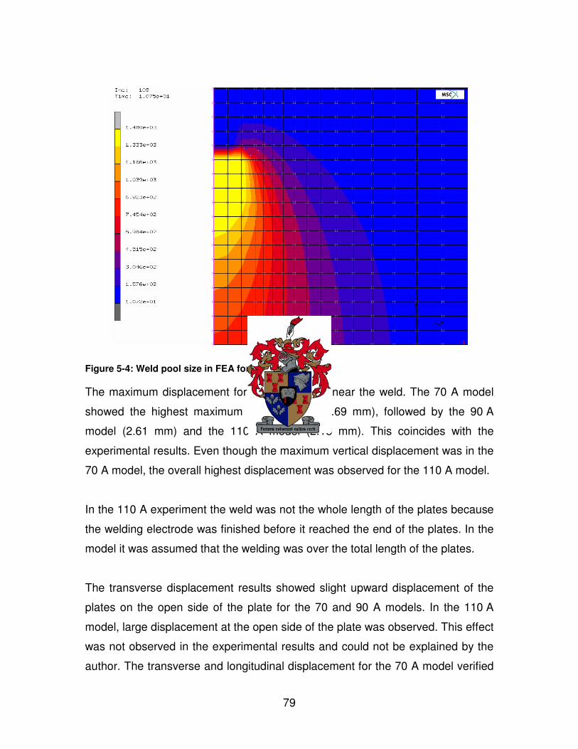
79
Figure 5-4: Weld pool size in FEA for 70 A model.
The maximum displacement for all models was near the weld. The 70 A model
showed the highest maximum displacement (2.69 mm), followed by the 90 A
model (2.61 mm) and the 110 A model (2.18 mm). This coincides with the
experimental results. Even though the maximum vertical displacement was in the
70 A model, the overall highest displacement was observed for the 110 A model.
In the 110 A experiment the weld was not the whole length of the plates because
the welding electrode was finished before it reached the end of the plates. In the
model it was assumed that the welding was over the total length of the plates.
The transverse displacement results showed slight upward displacement of the
plates on the open side of the plate for the 70 and 90 A models. In the 110 A
model, large displacement at the open side of the plate was observed. This effect
was not observed in the experimental results and could not be explained by the
author. The transverse and longitudinal displacement for the 70 A model verified

80
best with the experimental results for plate 2. The difference in displacement
results for the two plates in the experiments could be attributed to inaccuracies in
the experiments. This was discussed in more detail in Chapter 4.
0
0.5
1
1.5
2
2.5
3
3.5
4
4.5
0 50 100 150 200
Y [mm]
Dis
pla
cem
en
t [m
m]
FEM 70A EXP 70A P1 EXP 70A P2
Figure 5-5: Transverse displacement for 70A welding.
0
0.5
1
1.5
2
2.5
3
3.5
4
4.5
0 50 100 150 200
X [mm]
Dis
pla
cem
en
t [m
m]
FEM 70A EXP 70A P1 EXP 70A P2
Figure 5-6: Longitudinal displacement for 70A welding, 55mm from weld.

81
5.4.3 Experiment vs. FEM
The models did not converge to within an overall 80 % accuracy of the
experimental displacement results but did reveal agreement of tends. The points
of agreement between the experiments and FEA are discussed in this section.
With the verification of the experimental and modelling results, it was noticed that
everything from the experiments could not be modelled explicitly. This could have
led to inaccurate results. The design of the experiments was very robust and
more attention could have been focused on the retrieval of information. The
measuring technique used in the experiments was very robust and was used
because it was less time consuming.
The maximum displacements were observed close to the weld while the
distortion became less away from the weld. In lines parallel to the weldment
(longitudinal displacement) the plates bended upwards at the edges, resulting in
a parabolic shape of the plate (Figure 5-3 and Figure 5-6). In the 2 and 3 mm
cases (EXP) the maximum displacements was in the corner of the plate where
the welding finished while the in the 4 mm case the maximum displacement were
in the middle of the plate at the weldment.
The prediction of the location of the point of maximum displacement gave an
indication of the accuracy of the distortion modelling of the welded plates. The
most common point of maximum displacement in the experiments was measured
at the point closest to where the welding finished. Only the 3 mm model agreed
with the experiment. The 2 mm model predicted the maximum displacement at
the start of the welding and the 4 mm model in the middle of the plate on the
open side of the plate.
All three models investigating the effect of different welding current predicted the
maximum displacement of the plate correctly. These models also showed the
overall best agreement with welding tends.

82
In general, both the experiments and FEA agreed in parabolic shaped plates
parallel to the line of welding and the maximum displacement at the welding.
These results proved that the basic assumptions used in the models were correct
and laid a foundation for weld modelling.

83
6 CONCLUSION
The scope and objectives of the thesis to qualify for the MSc.Eng. degree
included:
• the development of a welding simulation using the finite element method,
• the verification of numerical results with those obtained in experiments
and
• the identification of the crucial parameters in weld modelling.
These objectives were successfully accomplished.
A literature survey was done on the welding process and prediction of welding
results in general. The survey was focused on temperature estimation, numerical
and analytical, and welding induced distortions. Guidelines proposed and used
by previous researchers were selected according to the specifications and
requirements of the model or weld. The use of two-dimensional in-plane weld
modelling had been accepted by various researchers as accurate
representations of the real welding process (Goldak, et al., 1986 and Deo, et al.,
2002). Based on the comments made by these researchers, the use of shell
elements for welding analysis was justified.
The use of temperature dependent material properties had been proved to be
crucial in the estimation of the temperature distribution of the plates. The greatest
limitation to computational weld mechanics was obtaining accurate temperature
dependent material properties (Goldak, et al., 1986). In cases where material
properties at elevated temperatures were not known, the properties of materials
with similar chemical content were used. Guidelines proposed for the calculation
of properties at elevated temperatures was also used (Zhu, et al., 2002).
Mild steel (SABS 1431 300WA) was used in the thesis because it was cheap,
had a good weldability and it was the most widely used metal in welding.

84
Shielded metal arc welding was used in the experiments. It was proved from the
experiments that the human welder gave repeatable results and welded at
optimal conditions. The parameters measured in the experiments were used as
input for the FE models. These parameters included the weld bead length,
welding speed and power input. The geometrical heat source parameters used in
the double ellipsoidal was taken from measurements of the weld bead. These
parameters were oversized with a factor less than 1.5 to obtain correct weld pool
size in the analysis.
The temperature results from the FE model were compared with the
experimental temperature results. The model parameters were changed within
the limits of the guidelines proposed by previous researchers until the results
were in acceptable tolerance of the experimental results. The element size,
material properties, volume weld flux, heat loss boundary conditions and analysis
options like the initial time step was experimented within the model until
satisfactory results were obtained.
Three-dimensional coupled analysis with contact as done and found to be time
consuming. The analysis was uncoupled and the nodal temperature history from
the thermal analysis was specified as a boundary condition in the structural
analysis. The three-dimensional analysis proved to be also time consuming and
inefficient. The welding was modelled with shell elements to save on computation
time.
The displacement magnitudes from the FEA models did not compare significantly
with the experiments, but the distortion tendencies observed in the experiments
were reflected in the models. The models were not valid to make accurate
distortion prediction but were sufficient to be used in welding feasibility case
studies and research.

85
6.1 Recommendations
The effect of the welding induced deformations was only investigated at local
area of the welding. Studies on the effects of welding on a complex structure can
to be investigated to determine the overall effect of the welding procedure on the
structure. This study will require the modelling of different weld geometries.
The available temperature dependent material properties were restricted and
innovative measures were taken to obtain these data. The thermo-physical
properties of mild steel at elevated temperatures can be investigated. The
metallurgical transformations of the steel during welding can be modelled to
determine the size and properties of the HAZ.
The simulation of other manufacturing processes like machining, forging, sheet
metal working and casting can be investigated. Little measurable financial impact
exists for modelling of manufacturing processes where the key elements of
successful modelling can be reviewed and to quantify the cost savings.

86
REFERENCES
Adak, M., Mandal, N.R., 2003, Thermo-Mechanical Analysis of Plates
Undergoing Line Heating Pseudolinear Equivalent Constant Rigidity System,
Transactions – Society of Naval Architects and Marine Engineers, v 111, p 353 –
361.
Adams, V., Askenazi, A., 1999, Building Better Products with Finite Element
Analysis, Onword Press, USA.
Audronis, M., Bendikas, J., 1983, The Welding Deformations of Chrome-Nickel
Stainless Steels, Material Science, Vol. 9, No. 2, p 169 – 173.
Bonifaz, E.A., 2000, Finite Element Analysis of Heat Flow in Single-Pass Arc
Welds, Welding Journal, v 79, p 121s – 125s.
Britsih Iron and Steel Research Association Metallurgy, 1953, Physical Constants
of Some Commercial Steels at Elevated Temperatures, London Butterworth
Scientific Publications.
Callister, W.D., 1997, Material Science and Engineering: An Introduction, John
Wiley and Sons, Inc., New York, USA.
Cook, R.D., 1995, Finite Element Modelling for Stress Analysis, John Wiley and
Sons, Inc., USA.
Dally, T.W., Riley, W.F., McConnell, K.G., 1993, Instrumentation for Engineering
Measurements, Second Edition, Wiley, New York, 1993.

87
Deo, M.V., Michaleris, P., Sun, J., 2002, Prediction of Buckling Distortion of
Welded Structures, Science and Technology of Welding and Joining.
Eagar, T.W., Tsai, N.S., 1983, Temperature Fields Produced by Travelling
Distributed Heat Sources, Welding Journal, v62, n12, p346 – 355.
Ericsson, M., 2003, Simulation of Robotic TIG-Welding, Department of
Technology, University of Trolhattan, Sweden.
Faure, W.C., Welding, Fabrication and Metal Work, Welding and Fabrication,
Bloemfontein, South Africa.
Francis, J.D., 2002, Welding Simulations of Aluminium Alloy Joints by Finite
Element Analysis, Master’s Thesis, Virginia Polytechnic Institute and State
University, Viginia, USA.
Fuersbach, P.W., Eisler, G.R., 2002, Determination of Material Properties for
Welding Models by Means of Arc Weld Experiments, 6th International Trends
Research, Pine Mountain, Georgia, USA.
Goldak, J., Chakravarti, A., Bibby, M., 1984, A New Finite Element Model for
Welding Heat Sources, Metallurgical Transactions B, Vol. 15B, p 299 – 305.
Goldak, J., Bibby, M., Moore, J., House, R., Patel, B., 1986, Computer Modeling
of Heat Flow in Welds, Metallurgical Transactions B, Volume 17B, p 587 – 600.
Groover, M.P., 1999, Fundamentals of Modern Manufacturing – Materials,
Processes and Systems, John Wiley and Sons, Inc, New York.
Hutton, D., Fundamentals of Finite Element Analysis, McGraw-Hill, New York,
2004.

88
Jang, C.D., Lee, C.H., 2003, Prediction of Welding Deformation of Ship Hull
Blocks, Proceedings of International Workshop on Frontier Technology in Ship
and Ocean Engineering.
Jung, G.H., Tsai, C.L., 2004, Fundamental Studies on the Effect of Distortion
Control Plans on Angular Distortion in Fillet Welded T-Joints, Welding Journal,
pp 213 – 223.
Kadivar, M.H., Jafarpur, K., Baradaran, G.H., 2000, Optimizing Welding
Sequence with Generic Algorithm, Computational Mechanics, v26, p 514 – 519.
Lancaster, J.F., 1965, The Metallurgy of Welding, Brazing and Soldering, George
Allen and Unwin Ltd, London.
Louhenkilpi, S., Markku, U., Kytonen, H., Vapalathi, S., 2003, Effect of
Thermophysical Material Data on Heat Transfer in Continuous Casting, Modelling
of Casting, Welding and Advanced Solidification Processes, pp 733 – 740.
Lourens, C., 2002, Wondermetal is poised to make inroads into the vehicle
sector, Industrial Reporter Business Day.
Luo, Y., Ishiyama, M., Murakawa, H., 1999, Welding Deformations of Plates with
Longitudinal Curvature, Transactions of Joining and Welding Research Institute,
Osaka, Japan, Vol. 28, No. 2.
Michaleris, P. and A. DeBiccari, 1996, Prediction of Welding Distortion, Welding
Journal, 76(4): 172s-180s
Michelaris, P., Feng, Z., Campbell, G., 1997, Evaluation of 2D and 3D FEA
Models for Predicting Residual Stress and Distortion, ASME PVP – Approximate

89
Methods in the Design and Analysis of Pressure Vessels and Piping
Components, 347, pp. 91 – 102.
Michaleris, P., Deo, M.V., 2002, Experimental Verification of Distortion Analysis
of Welded Stiffeners, Journal of Ship Production, 18(4):2 16-225.
Mills, A.F., 1995, Heat and Mass Transfer, Richard D. Irwin, Inc, USA.
Moshaiov, A., Eagar, T.W., 1990, Modelling of Distortion in Complex Structures,
Automation in the Design and Manufacture of Large Marine Systems, C.
Chryssostomidis ed., Hemisphere Publishing Corporation, New York.
Msc.Software Corporation, 2005, Msc.Marc Volume A: Theory and User
Information, Version 2005.
MSC.Software Corporation, 2003, MSC.Marc Introductory Course.
NAAMSA, 2003, New Vehicle Manufacturing Industry Data, www.naamsa.co.za,.
Phillips, A.L., 1968, Welding Handbook, Section One: Fundamentals of Welding,
American Welding Society, New York.
Pilipenko, A., 2001, Computer Simulation of Residual Stress and Distortion of
Thick Plates in Multi-Electrode Submerged Arc Welding. Their Mitigation
Techniques, Department of Machine Design and Materials Technology,
Norwegian University of Science and Technology, Norway
Tsai, C.L., Park, S.C., Cheng, W.T., 1999, Welding Distortion of a Thin-Plate
Panel Structure, Welding Journal, pp 156 – 165.

90
Tsai, N.S., Eagar, T.W., 1985, Distribution of the Heat and Current Fluxes in Gas
Tungsten Arcs, Metallurgical Transactions B, v16B, pp 841 – 846.
Weaver, M.A., 1999, Determination of Weld Loads and Throat Requirements
Using Finite Element Analysis with Shell Element Models – A Comparison with
Classical Analysis, Welding Journal, v78, n4, p 116s – 126s.
Wu, A., Syngellakis, S., Mellor, B.G., 2001, Finite Element Analysis of Residual
Stresses in a Butt Weld, Proceedings of the Seventh Postgraduate Conference in
Engineering Materials, p 37 – 38.
Zhu, X.K., Chao, Y.J., 2002, The Effect of Temperature-Dependent Material
Properties on Welding Simulation, Computers and Structures, Vol 80, pp 967 –
976.

91
APPENDIX A
A.1 Calculation of Natural Convection
Fluid motion past a surface increases the rate of heat transfer between the
surface and the fluid. A flowing fluid transports thermal energy by virtue of its
motion. As the air velocity increases, the isotherms move close together.
Isotherms are lines of constant temperature. Fourier’s law is not only valid in a
stationary solid, but it also applies in a moving fluid. Fourier’s law of heat
conduction states that in a homogeneous substance, the local heat flux is
proportional to the negative of the local temperature gradient (Mills, 1995):
0=∂
∂−=
y
sy
Tkq Equation A-1
As the isotherms move closer together and the temperature gradient normal to
the cylinder surface increases, so does the resulting heat conduction. The fluid in
contact with the cylinder is stationary due to viscous action and heat can be
transferred from the surface in the fluid by conduction only. The local heat
transfer rate is given by Equation A-2 (Mills, 1995).
Newton’s law of cooling defined the convective heat transfer coefficient by the
relation:
( )escs TThq −= Equation A-2
Combining Equations A-1 and A-2 give the convective heat transfer coefficient:
es
y
cTT
y
Tk
h−
∂
∂−
==0
Equation A-3

92
The effect of increasing the fluid velocity is to steepen the temperature gradient
at the surface, thereby increasing the heat transfer coefficient.
Natural convection, also known as free or buoyant convection occurs when
density differences due to heat differences take place and the earth’s
gravitational force produces a buoyancy force. Velocities associated with natural
convection are relatively small, not much more than 2 m/s. Convective heat
transfer coefficients tends to be low in the order of 5 W/m².°C (Mills, 1995).
For convective heat transfer dimensionless groups of pertinent variables are
used to organise experimental data for convective heat transfer coefficients. The
welded plates were assumed to be a heated plate facing up. The dimensionless
numbers needed to calculate the heat transfer coefficients were the Nusselt and
Rayleigh numbers. The Nusselt number, Nu, can be viewed as dimensionless
heat transfer coefficient in Equation A-4 and the Rayleigh number, Ra, was given
by Equation A-5.
k
LhNu c= Equation A-4
να
∆β 3TgLRa = Equation A-5
The convection input data in Patran/Marc in the convection load/BC’s menu
defines the film coefficient on faces of solid elements. The film coefficient is
defined as the convection coefficient for convective boundary conditions in
Patran. It can be entered either as a real constant or a reference to an existing
field definition. The film coefficient is user specified and is available from a
number of sources. Equation A-6 was for RaL > 107, turbulent thermals rise
irregularly above the plate and result in a Nusselt number independent of plate

93
size or shape. The Rayleigh number for the case of a welded plate was
calculated to be in the order of 1010.
31140
/LL Ra.Nu = ; 107
103102 ×<<× LRa Equation A-6
The heat transfer coefficient can be defined as a function of temperature by
substituting Equations A-4 and A-5 into Equation A-6 and the equation for hc for
free convection from a horizontal plate was given in Equation A-7.
31
31
140
/
/
c
g
k.
h
=να
ρ
ρ∆
Equation A-7
The heat transfer coefficient was specified in terms of the fluid’s physical
properties. Tables with temperature dependent data of these physical properties
were available (Mills, A.F., 1995) and the heat transfer coefficient as a function of
temperature is shown in Figure 2. These values may be conservative compared
to similar data found in the literature survey (Francis, J.D., 2002). Pilipenko used
a value of 30 W/m².K for the convective heat transfer coefficient which was much
higher than the values shown in Figure 2 (Pilipenko, A., 2001). The values in
Figure 2 were used in the simulation of the convective heat losses in the FE
modelling.

94
0
1
2
3
4
5
6
7
8
9
10
0 500 1000 1500 2000 2500 3000
Temperature [°C]
h [
W/m
².°C
]
Figure A-1: Convective heat transfer coefficient of heated horizontal plate.

95
APPENDIX B EXPERIMENTAL RESULTS
B.1 Effect of Restraints
B.1.1 Final Plate Transverse Displacement for Plate 1
Transverse Displacement: X = 10 mm
0
2
4
6
8
10
0 50 100 150 200
Y [mm]
h [
mm
]
Two Four Eight
Transverse Displacement: X = 55 mm
012345678
0 50 100 150 200
Y [mm]
h [
mm
]
Two Four Eight
Transverse Displacement: X = 100 mm
0
1
2
3
4
5
6
7
0 50 100 150 200
Y [mm]
h [
mm
]Two Four Eight
Transverse Displacement: X = 145 mm
012345678
0 50 100 150 200
Y [mm]
h [
mm
]
Two Four Eight
Transverse Displacement: X = 190 mm
0
2
4
6
8
10
0 50 100 150 200
Y [mm]
h [
mm
]
Two Four Eight

96
B.1.2 Final Plate Longitudinal Displacement for Plate 1
Longitudinal Displacement: 190 mm
from weld
0
1
2
3
4
5
6
7
0 50 100 150 200
X [mm]
h [
mm
]
Two Four Eight
Longitudinal Displacement: 145 mm
from weld.
0
2
4
6
8
0 50 100 150 200
X [mm]
h [
mm
]
Two Four Eight
Longitudinal Displacement: 100 mm
from weld
0
2
4
6
8
0 50 100 150 200
X [mm]
h [
mm
]
Two Four Eight
Longitudinal Displacement: 55 mm
from weld
0
2
4
6
8
10
0 50 100 150 200
X [mm]
h [
mm
]
Two Four Eight
Longitudinal Displacement: 10 mm
from weld.
0
2
4
6
8
10
0 50 100 150 200
X [mm]
h [
mm
]
Two Four Eight

97
B.1.3 Final Plate Transverse Displacement for Plate 2
Transverse Displacement: X = 10 mm
012345678
0 50 100 150 200
Y [mm]
h [
mm
]
Two Four Eight
Transverse Displacment: X = 55 mm
0
1
2
3
4
5
6
7
0 50 100 150 200
Y [mm]
h [
mm
]
Two Four Eight
Transverse Displacement: X = 100 mm
0
1
2
3
4
5
6
7
0 50 100 150 200
Y [mm]
h [
mm
]
Two Four Eight
Transverse Displacement: X = 145 mm
012345678
0 50 100 150 200
Y [mm]
h [
mm
]
Two Four Eight
Transverse Displacement: X = 190 mm
0
2
4
6
8
10
0 50 100 150 200
Y [mm]
h [
mm
]
Two Four Eight
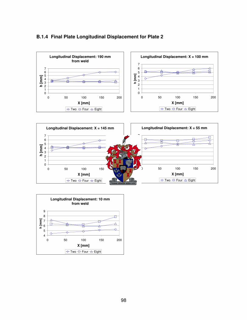
98
B.1.4 Final Plate Longitudinal Displacement for Plate 2
Longitudinal Displacement: 190 mm
from weld
01234567
0 50 100 150 200
X [mm]
h [
mm
]
Two Four Eight
Longitudinal Displacement: X = 145 mm
0
1
2
3
4
5
6
7
0 50 100 150 200
X [mm]
h [
mm
]
Two Four Eight
Longitudinal Displacement: X = 100 mm
0
1
2
3
4
5
6
7
0 50 100 150 200
X [mm]
h [
mm
]
Two Four Eight
Longitudinal Displacement: X = 55 mm
0
1
2
3
4
5
6
7
0 50 100 150 200
X [mm]
h [
mm
]
Two Four Eight
Longitudinal Displacement: 10 mm
from weld
4
5
6
7
8
9
0 50 100 150 200
X [mm]
h [
mm
]
Two Four Eight

99
B.2 Effects of Plate Thickness
B.2.1 Final Plate Transverse Displacement for Plate 1
Transverse Displacement: X = 10 mm
-2
0
2
4
6
8
0 50 100 150 200
Y [mm]
h [
mm
]
2mm 3mm 4mm
Transverse Displacement: X = 55 mm
-1
0
1
2
3
4
5
6
0 50 100 150 200
Y [mm]
h [
mm
]
2mm 3mm 4mm
Transverse Displacement: X = 100 mm
-1
0
1
2
3
4
5
6
0 50 100 150 200
Y [mm]
h [
mm
]
2mm 3mm 4mm
Transverse Displacement: X = 145 mm
0
1
2
3
4
5
6
0 50 100 150 200
Y [mm]
h [
mm
]
2mm 3mm 4mm
Transverse Displacement: X = 190 mm
01
2
34
56
78
0 50 100 150 200
Y [mm]
h [
mm
]
2mm 3mm 4mm

100
B.2.2 Final Plate Longitudinal Displacement for Plate 1
Longitudinal Displacement: 190 mm from weld
0
0.5
1
1.5
2
2.5
3
0 50 100 150 200
X [mm]
h [
mm
]
2mm 3mm 4mm
Longitudinal Displacement: 145 mm from weld
0
0.5
1
1.5
2
2.5
3
3.5
0 50 100 150 200
X [mm]
h [
mm
]
2mm 3mm 4mm
Longitudinal Displacement: 100 mm from weld
-1
0
1
2
3
4
5
0 50 100 150 200
X [mm]
h [
mm
]
2mm 3mm 4mm
Longitudinal Displacement: 55mm from weld
-101234567
0 50 100 150 200
X [mm]
h [
mm
]
2mm 3mm 4mm
Longitudinal Displacement: 10mm from weld
-2
0
2
4
6
8
0 50 100 150 200
X [mm]
h [
mm
]
2mm 3mm 4mm

101
B.2.3 Final Plate Transverse Displacement for Plate 2
Transverse Displacement: X = 10mm
-2
0
2
4
6
8
0 50 100 150 200
Y [mm]
h [
mm
]
2mm 3mm 4mm
Transverse Displacement: X = 55mm
-10123456
0 50 100 150 200
Y [mm]
h [
mm
]
2mm 3mm 4mm
Transverse Displacement: X = 100mm
-1
0
1
2
3
4
5
6
0 50 100 150 200
Y [mm]
h [
mm
]
2mm 3mm 4mm
Transverse Displacement: X = 145mm
-10
1
23
45
67
0 50 100 150 200
Y [mm]
h [
mm
]
2mm 3mm 4mm
Transverse Displacement: X = 190mm
-2
0
2
4
6
8
10
0 50 100 150 200
Y [mm]
h [
mm
]
2mm 3mm 4mm

102
B.2.4 Final Plate Longitudinal Displacement for Plate 2
Longitudinal Displacement: 190mm from weld.
-0.4-0.2
00.20.40.60.8
11.2
0 50 100 150 200
X [mm]
h [
mm
]
2mm 3mm 4mm
Longitudinal Displacement: 145mm from weld
-1-0.5
00.5
11.5
22.5
3
0 50 100 150 200
X [mm]
h [
mm
]
2mm 3mm 4mm
Longitudinal Displacement: 100mm from weld
-1
0
1
2
3
4
5
0 50 100 150 200
X [mm]
h [
mm
]
2mm 3mm 4mm
Longitudinal Displacment: 55mm from weld
-101234567
0 50 100 150 200
X [mm]
h [
mm
]
2mm 3mm 4mm
Longitudinal Displacement: 10mm from weld
-2
0
2
4
6
8
10
0 50 100 150 200
X [mm]
h [
mm
]
2mm 3mm 4mm

103
B.3 Effect of Heat Input
B.3.1 Final Plate Transverse Displacement for Plate 1
Trasnverse Displacement: X = 10mm
0.00
0.50
1.00
1.50
2.00
2.50
3.00
3.50
0 50 100 150 200
Y [mm]
h [
mm
]
70A 90A 110A
Transverse Displacement: X = 55mm
-0.50
0.00
0.50
1.00
1.50
2.00
2.50
3.00
0 50 100 150 200
Y [mm]
h [
mm
]
70A 90A 110A
Transverse Displacement: X = 100mm
-0.500.00
0.50
1.001.50
2.002.50
3.003.50
0 50 100 150 200
Y [mm]
h [
mm
]
70A 90A 110A
Transverse Displacement: X = 145mm
0.000.50
1.00
1.502.00
2.503.00
3.504.00
0 50 100 150 200
Y [mm]
h [
mm
]
70A 90A 110A
Transverse Displacement: X = 190mm
0.00
1.00
2.00
3.00
4.00
5.00
0 50 100 150 200
Y [mm]
h [
mm
]
70A 90A 110A

104
B.3.2 Final Plate Longitudinal Displacement for Plate 1
Longitudinal Displacement: X = 10mm
-0.500.000.501.001.502.002.503.003.504.00
0 50 100 150 200
Y [mm]
h [
mm
]
70A 90A 110A
Longitudinal Displacement: X = 55mm
0.000.50
1.00
1.502.00
2.503.00
3.504.00
0 50 100 150 200
Y [mm]
h [
mm
]
70A 90A 110A
Longitudinal Displacement: X = 100mm
0.00
1.00
2.00
3.00
4.00
5.00
0 50 100 150 200
Y [mm]
h [
mm
]
70A 90A 110A
Longitudinal Displacment: 145mm from weld
0.00
1.00
2.00
3.00
4.00
5.00
0 50 100 150 200
Y [mm]
h [
mm
]
70A 90A 110A
Longitudinal Displacement: 190 mm from weld
0.00
1.00
2.00
3.00
4.00
5.00
0 50 100 150 200
Y [mm]
h [
mm
]
70A 90A 110A

105
B.3.3 Final Plate Transverse Displacement for Plate 2
Transverse Displacement: X = 10mm
0.00
0.50
1.00
1.50
2.00
2.50
3.00
3.50
0 50 100 150 200
Y [mm]
h [
mm
]
70A 90A 110A
Transverse Displacement: X = 55mm
-0.500.00
0.50
1.001.50
2.002.50
3.003.50
0 50 100 150 200
Y [mm]
h [
mm
]
70A 90A 110A
Transverse Displacement: X = 100mm
-0.500.00
0.50
1.001.50
2.002.50
3.003.50
0 50 100 150 200
Y [mm]
h [
mm
]
70A 90A 110A
Transverse Displacment: X = 145mm
-1.00
0.00
1.00
2.00
3.00
4.00
0 50 100 150 200
Y [mm]
h [
mm
]
70A 90A 110A
Transverse Displacement: X = 190mm
0.00
1.00
2.00
3.00
4.00
5.00
0 50 100 150 200
Y [mm]
h [
mm
]
70A 90A 110A

106
B.3.4 Final Plate Longitudinal Displacement for Plate 2
Longitudinal Displacement: 190mm from weld.
-0.10
0.00
0.10
0.20
0.30
0.40
0 50 100 150 200
X [mm]
h [
mm
]
70A 90A 110A
Longitudinal Displacement: 145mm from weld
0.500.600.700.800.901.001.101.20
0 50 100 150 200
X [mm]
h [
mm
]
70A 90A 110A
Longitudinal Displacement: 100mm from weld
1.00
1.20
1.40
1.60
1.80
2.00
2.20
0 50 100 150 200
X [mm]
h [
mm
]
70A 90A 110A
Longitudinal Displacement: 55mm from weld
1.50
2.00
2.50
3.00
3.50
0 50 100 150 200
X [mm]
h [
mm
]
70A 90A 110A
Longitudinal Displacement: 10mm from weld
1.50
2.00
2.50
3.00
3.50
4.00
4.50
5.00
0 50 100 150 200
X [mm]
h [m
m]
70A 90A 110A

107
APPENDIX C EXPERIMENTAL TEMPERATURE RESULTS
C.1.1 Temperatures 30 mm from beginning of the weld
Temperature Distribution 20 mm from weld at X = 32
0
50
100
150
200
250
300
0 50 100 150 200 250 300
Time [s]
T [
°C]
Temperature Distribution 50 mm from weld at X = 30
20
30
40
50
60
70
80
90
0 100 200 300 400 500 600
Time [s]
T [
°C]
Temperature Distribution 150 mm from weld at X = 30
24
2628
3032
3436
3840
0 100 200 300 400 500 600
Time [s]
T [
°C]

108
C.1.2 Temperatures at 50 mm from the beginning of the weld
Temperature Distribution 20 mm from weld at X = 50
0
50
100
150
200
250
300
0 100 200 300 400 500 600
Time [s]
T [
°C]
Temperature Distribution 50 mm from weld at X = 50
20
40
60
80
100
120
0 100 200 300 400 500 600
Time [s]
T [
°C]
Temperature Distribution 150 mm from weld at X = 50
25
30
35
40
45
0 100 200 300 400 500 600
Time [s]
T [
°C]

109
C.1.3 Temperatures at 100 mm from beginning of weld
Temperature Distribution 20 mm from weld at X = 100
0
50
100
150
200
250
300
350
0 50 100 150 200 250 300
Time [s]
T [
°C]
Temperature distribution 50 mm from weld at X = 100
20
40
60
80
100
120
140
160
0 100 200 300 400 500 600
Time [s]
T [
°C]
Temperature Distribution 100 mm from weld at X = 100
25
30
35
40
45
0 100 200 300 400 500 600
Time [s]
T [
°C]

110
C.1.4 Temperature Distribution 20 mm From Weld
Temperatures 20 mm from weld
0
50
100
150
200
250
300
350
0 50 100 150 200 250 300
Time [s]
T [
°C]
X = 30
X = 50
X = 100 mm
Temperatures 50 mm from weld
20
40
60
80
100
120
140
160
0 100 200 300 400 500 600
Time [s]
T [
°C]
X = 30X = 50
X = 100
Temperatures 150 mm from weld
25
30
35
40
45
0 100 200 300 400 500 600
Time [s]
Tim
e [
s]
X = 30
X = 50
X = 100