finite-element em modelling on hexahedral grids with an fd

Geophys. J. Int. (2020) 223, 840–850 doi: 10.1093/gji/ggaa341Advance Access publication 2020 July 15GJI Marine geosciences and applied geophysics

Finite-element EM modelling on hexahedral grids with an FD solveras a pre-conditioner

Nikolay Yavich 1,2 and Michael S. Zhdanov2,3,4

1Skolkovo Institute of Science and Technology , CDISE, Moscow 143026, Russia. E-mail: [email protected] Institute of Physics and Technology Applied Computational Geophysics Lab, Dolgoprudny 141701, Russia3University of Utah Geology & Geophysics, Salt Lake City, UT 84112, USA4TechnoImaging LLC, Salt Lake City, UT 84107, USA

Accepted 2020 July 7. Received 2020 June 17; in original form 2019 July 26

S U M M A R YThe finite-element (FE) method is one of the most powerful numerical techniques for modelling3-D electromagnetic fields. At the same time, there still exists the problem of efficient andeconomical solution of the respective system of FE equations in the frequency domain. In thispaper, we concentrate on modelling with adapted hexahedral or logically rectangular grids.These grids are easy to generate, yet they are flexible enough to incorporate real topographyand seismic horizons. The goal of this work is to show how a finite-difference (FD) solver canbe used as a pre-conditioner for hexahedral FE modelling. Applying the lowest order Nedelecelements, we present a novel pre-conditioned iterative solver for the arising system of linearequations that combines an FD solver and simple smoothing procedure. The particular FDsolver that we use relies on the implicit factorization of the horizontally layered earth matrix.We assessed runtime and accuracy of the presented approach on synthetic and real resistivitymodels (topography of the Black Sea continental slope). We further compared performance ofour program versus publicly available Mare2DEM, ModEM and MUMPS programs/libraries.Our examples involve plane-wave and controlled source modelling. The numerical examplesdemonstrate that the presented approach is fast and robust for models with moderate contrast,supports highly deformed cells, and is quite memory-economical.

Key words: Controlled source electromagnetics (CSEM); Electromagnetic theory; Magne-totellurics; Numerical modelling; Numerical solutions.

1 I N T RO D U C T I O N

The role of 3-D electromagnetic (EM) forward modelling can hardlybe overestimated nowadays as it is used in EM survey design as wellas in EM data interpretation. In the frequency domain, the imple-mentation of a forward modelling routine generally involves thefollowing steps: computational grid generation, conductivity (andpossibly permittivity and susceptibility) averaging, system matrixpreparation, solution of the system of equations and interpolationof the solution to the receiver locations. In this paper, we addressthe problem of efficient solution of the finite-element (FE) systemof equations as it is the most computationally demanding step.

FE modelling on rectangular, more general hexahedral and tetra-hedral grids was discussed in a large number of relatively recentpublications (e.g. Silva et al. 2012; Cai et al. 2014, 2017; Li et al.2016, among many others); however, pre-conditioned iterative solu-tion is rarely considered, though we should note the work of Puzyrevet al. (2013), Um et al. (2013) and Ren et al. (2014).

Some authors studied the use of sparse direct solvers (Kordyet al. 2016) appealing to their universality and robustness. These

solvers require hundreds of Gb of auxiliary memory and hoursof CPU time at the factorization step for typical modelling. Withparallelization, this dramatic computational burden is somewhatreduced but remains significant.

To minimize the size of the FE system, grids with hanging nodesor octree grids can be used (Haber & Heldman 2007; Grayver &Kolev 2015). This kind of grids eliminates highly stretched cellsoutside the survey area. Although attractive in principle, solution ofthe respective system requires incorporation of a diffusion equationsolver, which ultimately raises computational complexity of a singleiteration.

Let us limit our consideration to adapted hexahedral gridsor logically rectangular grids (see Fig. 1a for 2-D illustration),that is, every cell in such a grid is received by finite deforma-tion of the respective cell of a rectangular grid (Fig. 1b). Log-ically rectangular grids directly accommodate land or seafloortopography or seismic horizons. It can be easily noted thatthe respective FE matrix shares many properties with the FEor finite-difference (FD) matrix constructed on the rectangulargrid.

840 C© The Author(s) 2020. Published by Oxford University Press on behalf of The Royal Astronomical Society.

Dow

nloaded from https://academ

ic.oup.com/gji/article/223/2/840/5871825 by U

niversity of Utah Eccles H

ealth Sciences Library user on 04 September 2020

http://orcid.org/0000-0002-8913-7710

mailto:[email protected]

Finite-element EM modelling on hexahedral grids 841

Figure 1. 2-D counterpart of an adapted (deformed) hexahedral grid or logically rectangular grid (a), (undeformed) rectangular grid (b), horizontally layeredearth model on the rectangular grid (c). Different filling pattern corresponds to conductivity values.

Figure 2. Six edges meeting at an internal node j of the hexahedral grid.

The key point of this paper is to check if an FD solver may beused as a pre-conditioner in FE modelling on logically rectangulargrids. As far as the authors are concerned, this type of solutionmethod was not published earlier. The particular FD solver that wewill test is based on the implicit and economical factorization ofthe horizontally layered earth matrix (Fig. 1c, see Appendix A orYavich et al. 2020).

This paper is organized as follows. At first, we formulate theFE system on a hexahedral grid. Next, we introduce FD matricesand discuss their relation to the FE system. After we describe asmoothing procedure, which happens to be necessary to warrantrobustness of the FD pre-conditioner for the FE problem. Finally, wepresent numerical examples that include both synthetic conductivitymodels, as a model with real marine topography. Our examplesinvolve plane-wave and controlled source modelling.

2 F I N I T E - E L E M E N T S Y S T E M O FE Q UAT I O N S

We consider a diffusion of EM field within 3-D heterogeneousconducting media with triaxial-anisotropic electrical conductivitytensor, σ (x, y, z):

σ (x, y, z) =⎛⎝

σx (x, y, z) 0 00 σy (x, y, z) 00 0 σz (x, y, z)

⎞⎠ . (1)

The conductivity is assumed to be non-zero in the air. Withinforward modelling, we look for the electric field E(x, y, z) thatsatisfies the following second-order system of partial differential

equations:

curl curl E − iωμ0σ E = iωμ0 J, (2)

where J is the source current density, i is the complex unity, ω

is the angular frequency and μ0 is magnetic permeability of thevacuum (Zhdanov 2002, 2009). These differential equations aresolved in a rectangular hexahedral computational domain V . Wefurther preferred secondary field modelling and thus complementedeq. (2) with zero Dirichlet boundary conditions,

E × ν = 0, (3)

where ν is the unit vector outward normal to the domain boundaryS.

We assumed that the computational domain is partitioned witha non-overlapping deformed hexahedral grid (see Fig. 1a) for a2-D illustration, and each cell will be denoted as Vj , j = 1..m.We further denote as n the number of internal edges. To find anapproximate solution to eqs (2) and (3) on the introduced grid,we follow the conventional FE technique. In this paper, we con-sidered lowest-order Nedelec FE basis functions (Nedelec 1986).For deformed hexahedra, they are completed by the covariant Pi-ola transform (Falk et al. 2011), which preserves continuity of thetangential components across interelement faces.

Using these basis functions, pk(x, y, z), k = 1..n, we expendthe unknown electric field, E, as follows:

E ≈n∑

k = 1

ekpk, e = (· · · ek · · · )T ∈ Cn . (4)

This discretization results in the following system of linear equa-tions:

A e = f, (5)

where A = R − iωμ0S, R = (Ri j ) , S = (Si j ), f = ( fi ) , i =1..n, j = 1..n,

Ri j = ∫V

curl pi · curl p j dV , Si j = ∫V

pi · σ p j dV ,

fi = iωμ0

∫V

pi · JdV .(6)

The obtained system is characterized by a large sparse complexsymmetric square matrix. The corresponding matrix equation canbe solved with both iterative and direct methods.

Dow





842 N. Yavich and M.S. Zhdanov

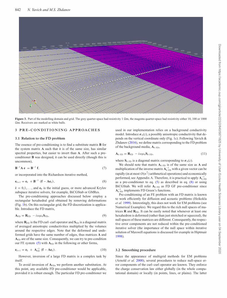
Figure 3. Part of the modelling domain and grid. The grey quarter-space had resistivity 1 �m, the magenta quarter-space had resistivity either 10, 100 or 1000�m. Receivers are marked as white balls.

3 P R E - C O N D I T I O N I N G A P P ROA C H E S

3.1 Relation to the FD problem

The essence of pre-conditioning is to find a substitute matrix B forthe system matrix A such that it is of the same size, has similarspectral properties, but easier to invert than A. After such a pre-conditioner B was designed, it can be used directly (though this isuncommon),

B−1A e = B−1 f, (7)

or incorporated into the Richardson iterative method,

ek+1 = ek + B−1 (f − Aek) , (8)

k = 0,1,. . . , and e0 is the initial guess, or more advanced Krylovsubspace iterative solvers, for example, BiCGStab or GMRes.

The pre-conditioning approaches discussed below employ arectangular hexahedral grid obtained by removing deformations(Fig. 1b). On this rectangular grid, the FD discretization is applica-ble. Introduce the FD matrix,

AFD = RFD − iωμ0SFD, (9)

where RFD is the FD curl–curl operator and SFD is a diagonal matrixof averaged anisotropic conductivities multiplied by the volumesaround the respective edges. Note that the deformed and unde-formed grids have the same number of edges, thus matrices A andAFD are of the same size. Consequently, we can try to pre-conditionour FE system (5) with AFD in the following or other forms,

ek+1 = ek + A−1FD (f − Aek) . (10)

However, inversion of a large FD matrix is a complex task byitself.

To avoid inversion of AFD, we perform another substitution. Atthis point, any available FD pre-conditioner would be applicable,provided it is robust enough. The particular FD pre-conditioner we

used in our implementation relies on a background conductivitymodel. Introduce σ b(z), a possibly anisotropic conductivity that de-pends on the vertical coordinate only (Fig. 1c). Following Yavich &Zhdanov (2016), we define matrix corresponding to the FD problemof the background media, Ab FD,

Ab FD = RFD − iωμ0Sb FD, (11)

where Sb FD is a diagonal matrix corresponding to σ b(z).We should note that matrix Ab FD is of the same size as A and

multiplication of the inverse matrix A−1b FD with a given vector can be

rapidly (in at most O(n43 ) arithmetical operations) and economically

performed, see Appendix A. Therefore, it is practical to apply A−1b FD

as a pre-conditioner to eq. (5) as described in eq. (8) or usingBiCGStab. We will refer Ab FD as FD GF pre-conditioner sinceA−1

b FD implements FD Green’s functions.Pre-conditioning of an FE problem with an FD matrix is known

to work efficiently for diffusion and acoustic problems (Heikoklaet al. 1999). Interestingly, this does not work for EM problems (seeNumerical Examples). We regard this to the rich null spaces of ma-trices R and RFD. It can be easily noted that whenever at least onehexahedron is deformed (rather than just stretched or squeezed), thenull spaces of these matrices are different. Consequently, the respec-tive error components are not reduced within the pre-conditionediterative solver (the importance of the null space within iterativesolution of Maxwell equations is discussed for example in Hiptmair1998).

3.2 Smoothing procedure

Since the appearance of multigrid methods for EM problems(Arnold et al. 2000), several procedures to reduce null-space er-ror components of the curl–curl operator are known. They enforcethe charge conservation law either globally (in the whole compu-tational domain) or locally (in points, lines, or plains). The latter

Dow






Figure 4. Electric field responses due to plane wave at 1 Hz for two-quarter-space model. Responses were computed using hexahedral FE program (Hex3D)and ModEM. The resistivity of the west quarter-space was 1 �m, the resistivity of east quarter-space was either 10, 100 or 1000 �m. (a)Ex component of theresponse due to x-polarized plane wave; b) Ey component of the response due to y-polarized plane wave.

Table 1. Iteration count and CPU time of hexahedral FE program (Hex3D)and ModEM. Iterative solver tolerance was 1e−7. The resistivity of the westquarter-space was 1 �m; the resistivity of east quarter-space was either 10,100 or 1000 �m.

East quarter-spaceresistivity (�m)

Hex3D Iterationcount/CPU time (min)

per polarizationModEM CPU time

(min) per polarization

10 58/2.86 3.86100 211/10.46 3.921000 433/21.71 3.92

Table 2. Iteration count and CPU time of hexahedral FE program (Hex3D)for a sequence of grids. Iterative solver tolerance was 1e−7. The resistivityof the west quarter-space was 1 �m; the resistivity of east quarter-space was100 �m.

Modelling grid Discrete problem size

Hex3D Iterationcount/CPU time (min)

per polarization

136 × 56 × 75 1 669 835 211/10.4668 × 28 × 37 200 565 197/0.8034 × 14 × 18 23 090 142/0.03

Dow






Figure 5. Model with simple seafloor bathymetry: sea-water layer (grey), sediments (red), source (leftmost white disk) and receivers (the other white disks).The modelling grid was adapted to the seafloor (blue lines).

Figure 6. BiCGStab convergence history pre-conditioned with either Ab FD matrix only (GF), or combined with pre-smoothing (S + GF), or pre- andpost-smoothing (S + GF + S) for the model with simple seafloor bathymetry

Table 3. Performance of the BiCGStab solver pre-conditioned with eitherAb FD matrix only (GF), or combined with pre-smoothing (S + GF), orpre- and post-smoothing (S + GF + S) for the model with simple seafloorbathymetry.

Pre-conditionedBiCGStab solver

Iterationcount

CPU time(min)

CPU time (min)per iteration

S + GF + S 6 0.16 0.026S + GF 9 0.17 0.019GF 16 0.22 0.014

procedures are referred to as smoothers within multigrid methodsbecause they smooth out spatial error components.

The smoothing procedure that has the smallest arithmetical com-plexity performs point smoothing in the block Jacobi fashion. Letp be the number of internal grid nodes. At any internal node ofa logically rectangular hexahedral grid, six edges meet (Fig. 2).Consider a node j . Let B j be an n × n matrix that coincideswith A at those columns and rows which correspond to the sixedges, while coinciding with the identity matrix at the rest of theentries.

Dow






Figure 7. Real and imaginary parts of the inline electric field components tangential to the seafloor. Hexahedral FE modelling (Hex3D) compared with 2-DFE modelling (M2D) of mare2DEM for the model with simple seafloor bathymetry

Note that the matrix B j is easy to invert and solution of a systemwith matrix B j enforces the charge conservation law in the point j .Now, the block Jacobi smoother can be written as follows:

ek+1 = ek + η

p∑j = 1

B−1j (f − A ek) . (12)

This procedure has linear arithmetical complexity and naturallyparallelizable. The scalar parameter η should be positive and lessthan 1. In our experiments, we picked η = 0.5 as this choice takesin account the fact that each edge is involved at most twice in thestencils, Fig. 2. (Yavich & Scholl 2012).

Now we have to combine the pre-conditioning step (eqs 10 and11) with the smoothing step (eq. 12). The next three-step algorithm

resulted in a robust solver,

ek+1/3 = ek + ηp∑

j = 1B−1

j (f − A ek) ,

ek+2/3 = ek+1/3 + A−1b F D

(f − A ek+1/3

),

ek+1 = ek+2/3 + ηp∑

j = 1B−1

j

(f − A ek+2/3

).

(13)

Practically, we do not implement eq. (13) as is, rather thesethree steps were implemented as a pre-conditioner to the BiCGStabiterative solver. Following the multigrid terminology, the first stepwe will be referred to as pre-smoothing, the last step we will bereferred to as post-smoothing.

Dow






Figure 8. Seafloor bathymetry.

To wrap up this section, let us summarize the properties of thedesigned pre-conditioner. Arithmetical complexity of a single ap-plication of eq. (13) is O(n

43 ). Initialization is momentary since it

involves manipulation with 1-D discrete problems only, needed toprepare for multiplication of A−1

b FD by a vector. Inversion of 6 × 6block arising in B−1

j is performed on-the-fly to minimize storageexpenses.

4 N U M E R I C A L E X A M P L E S

In this section, we present the results of 3-D numerical modelling ex-periments with the pre-conditioning scheme (13) introduced earlier.The scheme was incorporated into the BiCGStab iterative solver.The finite-element system of equations (5) was implemented inMatlab (program of Cai et al. 2014). The finite-difference pre-conditioner introduced in eq. (11) (Yavich & Zhdanov 2016) andsmoother (12) were implemented in C/C++ and linked to the Mat-lab code. Computations were performed on a Linux cluster node.All the presented results involve sequential computations.

4.1 Modelling on rectangular grids

We start off our experiments with a simple model (Fig. 3) consistingof two quarter-spaces of different resistivity. The west (x < 0) hasresistivity 1 �m, while the resistivity of the east quarter-space (x >

0) was different in different tests, 10, 100 and 1000 �m, respectively.A plane-wave electric field response at 1 Hz was recorded along a12 km profile, perpendicular to the contact interface. The resistivityof the air was 106 �m.

In this case, we used an FE grid that matched the FD grid. Themodelling domain occupied the volume [−85; 85] × [−80; 80] ×[−53; 71] km3 and cells in the central part had the size 125 × 125× 50 m3. Part of the grid is shown in Fig. 3. The grid had 136 × 56× 75 cells, making the discrete problem size 1 669 835 unknowns.

We compared accuracy and runtime of our program versus thoseof ModEM 2019, Egbert & Kelbert (2012) and Kelbert et al. (2014).ModEM has implemented Fortran 95 and its solver part combinesQMR iterations with ILU pre-conditioner and static divergence cor-rections. ModEM supports transfer function computation only, thusminor edits were implemented to obtain the electric fields due to aparticular polarization.

Both of the programs used the same modelling grid and accu-racy of the iterative solvers was set to 1e−7. Fig. 4 illustrates the

computed responses by the two programs for the three differentresistivities of the east quarter-space. The Ex component of the re-sponse due to x-polarized plane wave is shown in Fig. 4(a), whileEy component of the response due to y-polarized plane wave isshown in Fig. 4(b). The electric fields were normalized so that theywould pass through the unity at x = 0.

We observe a fairly good match of the responses. Though, somediscrepancies are notable in the 1000 �m case. We regard thisto different incorporation of the quarter-space: our program usessecondary field modelling, while ModEM uses primary field mod-elling.

Smoothing was not applied in this test since hexahedrons werenot deformed. Table 1 presents iteration count and CPU time of ourhexahedral FE program and ModEM. Our program was faster incase of moderate resistivity contrast, while in other cases, the num-ber of iterations tends to grow. For this model, the pre-conditioningmatrix Ab FD corresponds to a uniform half-space model. Conse-quently, this approach loses robustness. On the other hand, ModEMperforms fairly invariant to resistivity increase. We should notethat our program is experimental and involves Matlab code, nev-ertheless, in some cases, its performance is competitive with theindustry-standard program.

We also investigated the impact of the discrete problem sizein Table 2. The originally generated grid 136 × 56 × 75 wascoarsened either two or four times in each direction by remov-ing the respective grid lines. The table reports iteration count andCPU time required for modelling with these grids. We see thatthe grid size has a small impact on the iteration count, imply-ing that the resented approach is applicable for large-scale prob-lems.

4.2 Simple bathymetry modelling

In this section, we illustrate performance of the designed algorithmapplied for marine CSEM modelling in the presence of 2-D simpleseafloor topography. We considered a model formed by a 1000 mdeep sea-water layer and of 0.3 �m and homogenous seafloor of1 �m. The seafloor contains an elevation of 110 m uniform inthe y-direction (Fig. 5). The top of the elevation is located alongx = 0 and it spans approximately from x = −500 m to x =500 m.

We modelled a response of a x-directed dipole source centred in[−1500; 0; 900] m, that is, 100 m above the seafloor and 1.5 kmto the west of the elevation. The source was emitting at 1 Hz. Theseafloor receivers were inline to the source, along y = 0 andtangential to the seafloor.

For this set-up, a hexahedral grid was generated. The modellinggrid covered the volume [−3; 4] × [−3; 3] × [−5; 3] km3, had thesmallest cell size 100 × 100 × 50 m3 and was adapted to seafloortopography (Fig. 5). The grid had dimensions 70 × 36 × 81, makingthe size of the discrete problem 590 335.

Fig. 6 shows BiCGStab convergence history pre-conditioned witheither Ab FD matrix (11) only, or combined with pre-smoothing, orpre- and post-smoothing (13). See also Table 3. In all of the threecases, the iterative solver converged to the target residual of 1e−7quite fast: 16, 9 and 6 iterations respectively. Though, we shouldnote that the use of smoothing increased convergence speed con-siderably. Also, note that smoothing steps increased computationalcomplexity of a single iteration (Table 3). Nevertheless, the shortestCPU time was received when two smoothing steps were performedper iteration.

Dow






Figure 9. Hexahedral grid adapted to seafloor bathymetry. The source is marked as a blue ball, receivers are marked as white balls.

Figure 10. BiCGStab convergence pre-conditioned with FD GF completed with either no smoothing (GF), pre-smoothing (S + GF) or pre- and post-smoothing(S + GF + S).

Table 4. Performance of the pre-conditioned iterative and sparse directsolvers.

Solver CPU timePeak memory

usage

BiCGStab/S + GF + S 5.3 min 1 GbMUMPS factorize 8.0 hr

solve 0.7 min56 Gb

To conclude this experiment, we illustrate and compare the com-puted response with that of publicly available program 2.5-D finite-element code Mare2DEM (Key 2016). We should note that themodel used in this experiment is 2-D with y being the strike direc-tion, consequently such a comparison is fair. Fig. 7 shows real andimaginary parts of the electric field components. We observe a goodmatch, though some inaccuracies are notable near sign reversals.

Dow






Figure 11. Responses computed with the pre-conditioned iterative and sparse direct solvers. Real and imaginary parts of the inline electric field componenttangential to the seafloor are shown.

4.3 Real bathymetry modelling

We modelled a response of a horizontal electric dipole of 1 Hz towednear the seafloor. We assumed a homogeneous 1 �m subsurface,while seafloor bathymetry represents an 8 × 8 km2 area of the BlackSea continental slope (Daudina et al. 2014; Yavich et al. 2019),Fig. 8. In this area, depth varies from 450 to 1150 m. Sea-waterconductivity was 0.3 �m.

For this set-up, we generated a non-uniform 115 × 100 × 55 grid(Fig. 9) with overall 1.851 million discrete electric field unknowns.The grid was adapted to the seafloor bathymetry.

Fig. 10 illustrates convergence of the BiCGStab iterative solver,pre-conditioned with Ab FD completed with either no smooth-ing, pre-smoothing or pre- and post-smoothing. In the last case,the pre-conditioned iterative solver converged in 53 iterationsin 5.3 min to the residual norm of 1e−6. In other cases, noconvergence was observed. We conclude that for realistic mod-els, pre- and post-smoothing are necessary to gain robustness.Note that both smoothing and the FD GF pre-conditioner arenaturally parallelizable (Yavich & Scholl 2012; Yavich et al.2017).

Finally, we linked to the commonly used MUMPS sparse directsolver (Amestoy et al. 2001) to assess their performance versus thediscussed approach. In this study, we have looked at sequential per-formance leaving investigation of scalability aside. MUMPS 5.1.1was used and complex symmetricity of the matrix was employedduring factorization.

Table 4 shows CPU time and memory usage of the pre-conditioned iterative and MUMPS sparse direct solvers. It took8 hr and 56 Gb of memory for the direct solver to factorize thematrix. In contrast, the designed pre-conditioned iterative solver re-quired only near 1 Gb of memory. We conclude that in this example,the iterative solver was roughly 90 times faster and 50 times morememory-economical.

Both of the approaches can gain some speedup in a parallelenvironment, but the computational burden of the sparse directfactorization still will be significant.

Finally, Fig. 11 illustrates responses modelled with the twosolvers. The responses are essentially identical. This demonstratesthe fact that pre-conditioning eqs (10) and (12) corresponds to theequivalent transformation of the original linear system (5).

5 C O N C LU S I O N S

We designed and tested a pre-conditioning scheme for the hexahe-dral FE system of equations resulting from the discretization on alogically rectangular grid. The approach combines the FD GF pre-conditioner and pre- and post-smoothing procedures. Accuracy andruntime were compared versus commonly used in the EM commu-nity programs ModEM and Mare2DEM. The numerical examplespresented above demonstrate that the presented approach is fast androbust for models with moderate contrast. As far as the authors areconcerned, this type of pre-conditioning has not been published ear-lier. An attempt to further leverage the presented approach with thecontraction-operator transformation, which can potentially furtheraccelerate FE forward modelling, will be performed. Another wayto gain robustness would be to substitute point smoothing with linesmoothing (Mulder 2006).

Arbitrary unstructured tetrahedral and hexahedral grids or gridswith hanging nodes presumably cannot be used with the presentedapproach. Our consideration was limited to lowest order Nedelec ba-sis functions for logically rectangular grids, while the developed pre-conditioner can be directly reused for higher-order basis functions.We will also try to reuse this approach for time-domain modelling,where accurate incorporation of land topography is of paramountimportance.

A C K N OW L E D G E M E N T S

The authors acknowledge the Skoltech, MIPT, University of Utah’sConsortium for Electromagnetic Modeling and Inversion (CEMI)and TechnoImaging for help with this research and permissionto publish. The authors appreciate fruitful discussions with their

Dow






colleagues, Drs Hongzhu Cai, Mikhail Malovichko and PavelPushkarev. We also thank Drs G. Egbert and A. Kelbert for theopportunity to use ModEM software in this study. We would liketo appreciate the Skoltech CDISE’s high-performance computingcluster, Zhores (Zacharov et al. 2019), for providing the computingresources that have contributed to the results reported herein.

This research was supported by the Russian Science Foundation,project No. 18-71-10071.

R E F E R E N C E SAmestoy, P.R., Duff, I.S., Koster, J. & L’Excellent, J.-Y., 2001. A fully

asynchronous multifrontal solver using distributed dynamic scheduling,SIAM J. Matrix Anal. Appl., 23, 15–41.

Arnold, D.N., Falk, R.S. & Winther, R., 2000. Multigrid in H(div) andH(curl), Numer. Math., 85, 197–217.

Cai, H., Xiong, B., Han, M. & Zhdanov, M., 2014. 3D controlled-sourceelectromagnetic modeling in anisotropic medium using edge-based finiteelement method, Comput. Geosci., 73, 164–176.

Cai, H., Hu, X., Li, J., Endo, M. & Xiong, B., 2017. Parallelized 3D CSEMmodeling using edge-based finite element with total field formulation andunstructured mesh, Comput. Geosci., 99, 125–134.

Da Silva, N.V., Morgan, J.V., MacGregor, L. & Warner, M., 2012, A finiteelement multifrontal method for 3D CSEM modeling in the frequencydomain, Geophysics, 77(2), E101–E115.

Daudina, D., Malovichko, M., Myasoedov, N., Nikishin, A., Poludetkina,E., Tikhotskiy, S. & Tokarev, M., 2014. Joint inversion of multi-typegeophysical and geochemical data for hydrocarbon systems explorationat sea shelf, in 6th EAGE Saint Petersburg International Conference andExhibition, https://doi.org/10.3997/2214-4609.20140152.

Egbert, G.D. & Kelbert, A., 2012. Computational recipes for electromagneticinverse problems, Geophys. J. Int., 189(1), 251–267.

Falk, R.S., Gatto, P. & Monk, P., 2011. Hexahedral H(div) and H(curl) finiteelements, ESAIM: M2AN, 45(1), 115–143.

Grayver, A.V. & Kolev, Tz.V., 2015, Large-scale 3D geoelectromagneticmodeling using parallel adaptive high-order finite element method,Geophysics, 80(6), E277–E291.

Haber, E. & Heldmann, S., 2007. An octree multigrid method for quasi-staticMaxwell’s equations with highly discontinuous coefficients, J. Comput.Phys., 223(2), 783–796.

Heikkola, E., Kuznetsov, Y.A. & Lipnikov, K.N., 1999, Fictitious domainmethods for the numerical solution of three-dimensional acoustic scatter-ing problems, J. Comput. Acoust., 7(3), 161–183.

Hiptmair, R., 1998. Multigrid method for Maxwell’s equations, SIAM J.Numer. Anal., 36(1), 204–225.

Kelbert, A., Meqbel, N., Egbert, G.D. & Tandon, K., 2014. ModEM: a mod-ular system for inversion of electromagnetic geophysical data, Comput.Geosci., 66, 40–53.

Key, K., 2016. MARE2DEM: a 2-D inversion code for controlled-sourceelectromagnetic and magnetotelluric data, Geophys. J. Int., 207(1), 571–588.

Kordy, M., Wannamaker, P., Maris, V., Cherkaev, E. & Hill, G., 2016. 3-Dmagnetotelluric inversion including topography using deformed hexahe-dral edge finite elements and direct solvers parallelized on SMP computers– Part I: forward problem and parameter Jacobians, Geophys. J. Int., 204,74–93.

Li, J., Farquharson, C.G. & Hu, X., 2016. 3D vector finite-element elec-tromagnetic forward modeling for large loop sources using a total-fieldalgorithm and unstructured tetrahedral grids, Geophysics, 82(1), E1–E16.

Mulder, W.A., 2006, A multigrid solver for 3D electromagnetic diffusion,Geophys. Prospect., 54, 633–649.

Nedelec, J.-C., 1986. A new family of mixed finite elements in R3, Numer.Math., 50(1), 57–81.

Puzyrev, V., Koldan, J., de la Puente, J., Houzeaux, G., Vazquez, M. &Cela, J.M., 2013, A parallel finite-element method for three-dimensionalcontrolled-source electromagnetic forward modelling, Geophys. J. Int.,193(2), 678–693.

Ren, Zh., Kalscheuer, Th., Greenhalgh, St. & Maurer, H., 2014, A finite-element-based domain-decomposition approach for plane wave 3D elec-tromagnetic modeling, Geophysics, 79(6), E255–E268.

Um, E.S., Commer, M. & Newman, G.A., 2013. Efficient pre-conditionediterative solution strategies for the electromagnetic diffusion in the Earth:finite-element frequency-domain approach, Geophys. J. Int., 193(3),1460–1473.

Yavich, N. & Scholl, C., 2012. Advances in multigrid solution of 3D forwardMCSEM problem, in 5th EAGE St. Petersburg International Conferenceand Exhibition on Geosciences, EAGE. https://doi.org/10.3997/2214-4609.20143665

Yavich, N. & Zhdanov, M., 2016. Contraction pre-conditioner in finite-difference electromagnetic modelling, Geophys. J. Int., 206, 1718–1729.

Yavich, N., Malovichko, M., Khokhlov, N. & Zhdanov, M., 2017. Advancedmethod of FD electromagnetic modeling based on contraction operator,79th EAGE Conference and Exhibition, https://doi.org/10.3997/2214-4609.201701354.

Yavich, N., Malovichko, M. & Zhdanov, M., 2019, Towards efficient finite-element EM modeling on hexahedral grids, 81st EAGE Conference andExhibition, https://doi.org/10.3997/2214-4609.201901487.

Yavich, N., Malovichko, M. & Shlykov, A., 2020. Parallel simulation ofaudio- and radio-magnetotelluric data, Minerals, 10(1), 42.

Zacharov, I. et al. 2019. “Zhores”—Petaflops supercomputer for data-driven modeling, machine learning and artificial intelligence installedin Skolkovo Institute of Science and Technology, Open Eng., 9, 512–520.

Zaslavsky, M., Druskin, V., Davydycheva, S., Knizhnerman, L., Abubakar,A. & Habashy, T., 2011, Hybrid finite-difference integral equationsolver for 3D frequency domain anisotropic electromagnetic problems,Geophysics, 76(2), F123–F137.

Zhdanov, M., 2002. Geophysical Inverse Theory and Regularization Prob-lems. Elsevier.

Zhdanov, M., 2009, Geophysical Electromagnetic Theory and Methods. El-sevier.

A P P E N D I X A : FA S T I N V E R S I O N O F Ab FD

In this appendix, we describe an approach for direct factorizationof matrix Ab FD, an FD matrix corresponding to Maxwell equationsin a possibly anisotropic medium of conductivity σ b(z). Eq. (2) inthis case read as follows in explicit form:

−∂2 Ex

∂y2− ∂2 Ex

∂z2+ ∂2 Ey

∂x∂y+ ∂2 Ez

∂x∂z− iωμ0σbx (z)Ex = iωμ0 Jx ,

−∂2 Ey

∂x2− ∂2 Ey

∂z2+ ∂2 Ex

∂x∂y+ ∂2 Ez

∂y∂z− iωμ0σby(z)Ey = iωμ0 Jy,

−∂2 Ez

∂x2− ∂2 Ez

∂y2+ ∂2 Ex

∂x∂z+ ∂2 Ey

∂y∂z− iωμ0σbz(z)Ez = iωμ0 Jz .

(A1)

We assume that the non-uniform FD grid is formed by Nx ×Ny × Nz cells. In complexity and size estimates, we assume thenumbers of grid cells in all directions are of the same order. We willpresent an algorithm to efficiently solve

Ab FDv = g (A2)

for v while g ∈ Cn is given. For magnetic field modelling on Lebe-

dev grids, a similar algorithm was presented in Zaslavsky et al.(2011). The below-described approach is analogous to using doubleFourier transform for solution of differential equation system (A1).

Matrix Ab FD inherits the structure of eq. (A1). It can be presentedin the following way:

Ab FD =⎛⎝

Axx Axy Axz

Ayx Ayy Ayz

Azx Azy Azz

⎞⎠ . (A3)

Dow





http://dx.doi.org/10.1137/S0895479899358194

http://dx.doi.org/10.1007/PL00005386

http://dx.doi.org/10.1016/j.cageo.2014.09.008


http://dx.doi.org/10.1190/geo2010-0398.1

https://doi.org/10.3997/2214-4609.20140152

http://dx.doi.org/10.1111/j.1365-246X.2011.05347.x

http://dx.doi.org/10.1051/m2an/2010034


http://dx.doi.org/10.1016/j.jcp.2006.10.012

http://dx.doi.org/10.1142/S0218396X99000126

http://dx.doi.org/10.1137/S0036142997326203


http://dx.doi.org/10.1093/gji/ggw290

http://dx.doi.org/10.1093/gji/ggv410


http://dx.doi.org/10.1111/j.1365-2478.2006.00558.x

http://dx.doi.org/10.1007/BF01389668

http://dx.doi.org/10.1093/gji/ggt027


http://dx.doi.org/10.1093/gji/ggt071

https://doi.org/10.3997/2214-4609.20143665

http://dx.doi.org/10.1093/gji/ggw237

https://doi.org/10.3997/2214-4609.201701354

https://doi.org/10.3997/2214-4609.201901487

http://dx.doi.org/10.3390/min10010042

http://dx.doi.org/10.1515/eng-2019-0059

http://dx.doi.org/10.1190/1.3552595


We will use a special representation of matrix Ab FD. To introduceit, we need some auxiliary notations. Note that discretization of eq.(A1) involves backward, forward and central FE operators. The

Kronecker product (Appendix B) will let us write components ofAb FD explicitly,

Axx = I zd ⊗ Ay

d ⊗ I xn + Az

d ⊗ I yd ⊗ I x

n − iωμ0�x ⊗ I y

d ⊗ I xn ,

Axy = I zd ⊗ F y

dn ⊗ F xnd ,

Axz = I zdn ⊗ I y

d ⊗ F xnd ,

· · ·Azz = I z

n ⊗ Ayd ⊗ I x

d + I zn ⊗ I y

d ⊗ Axd − iωμ0�

Z ⊗ I yd ⊗ I x

n .

(A4)

Here, I xd , I y

d , etc., are identity matrices; �x , � y and �z are diago-nal matrices corresponding to σbx (z), σby(z) and σbz(z), respectively;F x

nd and F ydn are backword and forward difference operators result-

ing from discretization of ∂2

∂x∂y ; matrices Axd , etc., correspond to

discretization of ∂2

∂x2 . An important feature of all the matrices in-volved in the right-hand side of eq. (A4) is that they are eitherdiagonal, bidiagonal or tridiagonal. Also they are relatively smallin size, O(Nx ), since they correspond to 1-D ordinary differentialoperators. However, the blocks Axx , etc., are large and have a largeband.

We will now simplify the structure of Ab FD and invert it usingspectral and singular value decompositions of earlier introducedmatrices Ax

d , F xnd , etc. This is achieved in three steps.

Step 1–Symmetrization. Matrix Ab FD is not symmetric generally.We can symmetrize it by using a diagonal matrix,

D = diag(Dz

d ⊗ Dyd ⊗ Dx

n , Dzd ⊗ Dy

n ⊗ Dxd ,

Dzn ⊗ Dy

d ⊗ Dxd

). (A5)

Here, Dxd , etc., are diagonal matrices of grid steps in the respective

directions. Now we can put,

A = D12 Ab FD D− 1

2 . (A6)

Now solving (A2) is equivalent to solving

A v = g , (A7)

with

v = D12 v, g = D

12 g. (A8)

After this scaling, matrix A is always symmetric.Step 2–Diagonalization. Matrices involved in A can now be di-

agonalized using eigenvalue decomposition. At this step we diag-onalize those matrices that correspond to FD differentiation in thehorizontal direction. The respective eigenvector basis is denoted asW x

d , W yd , etc. Define,

W = diag(I z

d ⊗ W yd ⊗ W x

n , I zd ⊗ W y

n ⊗ W xd ,

I zn ⊗ W y

d ⊗ W xd

).

(A9)

and put

T = WT A W. (A10)

Matrix T benefits from the eigenvector basis and has the followingform:

T =⎛⎝

Txx Txy Txz

Tyx Tyy Tyz

Tzx Tzy Tzz

⎞⎠ , (A11)

Txx = I zd ⊗ �

yd ⊗ I x

n + Azd ⊗ I y

d ⊗ I xn − iωμ0�

x ⊗ I yd ⊗ I x

n ,

Txy = −I zd ⊗ (�y

nd )12 T ⊗ (�x

nd )12 ,

Txz = −Fzdn ⊗ I y

d ⊗ (�xnd )

12 ,

· · ·Tzz = I z

n ⊗ �yd ⊗ I z

d + I zn ⊗ I y

d ⊗ �xd − iωμ0�

z ⊗ I yd ⊗ I x

n .

(A12)

Switching from A to T in (A7) gives us,

T u = f, f = WT g, u = WT v. (A13)

An important feature of the above matrix is that all FD derivativeswith respect to x and y are gone. All of the nine blocks of T areeither diagonal, bidiagonal or tridiagonal. Consequently, we canfactorize it efficiently (see the next step).

Step 3–Factorization. In order to solve eq. (A13), it remains todiscuss an approach to factorize T. As it was noted above, matrixT involves only FD derivatives with respect to z. Further note thatTzz block is diagonal. Consequently, we can eliminate the respectivesubset of unknowns while keeping sparsity of the remaining blocksof the matrix. Under an appropriate renumbering, the obtained ma-trix will be block diagonal with O(Nx Ny) blocks and each blockbeing a symmetric seven-diagonal matrix of size O(Nz). Thus, wecan factorize every block using L DLT -algorithm in linear time.This is performed on-the-fly.

Solution of eq. (A2) can be summarized as follows: apply diag-onal scaling D (A8), then perform conversion to the eigenvaluebasis (A13), after this, find the discrete harmonics, then performconversion from the eigenvalue basis, and finally remove diagonalscaling.

All the operations performed in the algorithm above are linearwith respect to the problem size n except conversions from/to theeigenvalue basis which require O(Nz Nx Ny(Nx + Ny)) or O(n

43 )

operations. Thus, the latter complexity dominates in the solutionof eq. (A2). At initialization, eigenvalue decomposition of fourtridiagonal matrices is performed. The overall complexity of thisstep is O (n2

x ) = O(n23 ).

A P P E N D I X B : K RO N E C K E R P RO D U C TA N D I T S P RO P E RT I E S

Given an m × n matrix A = {ai j } and some matrix B, their Kro-necker product matrix A ⊗ B is a block matrix defined as

A ⊗ B =⎛⎝

a11 B · · · a1n B· · ·

am1 B · · · amn B

⎞⎠ . (B1)

We used the following properties of this product within this note:

(A ⊗ B )T = AT ⊗ BT , (B2)

(A ⊗ B )−1 = A−1 ⊗ B−1, (B3)

(A ⊗ B) (C ⊗ D) = (AC) ⊗ (BD) . (B4)

The identity (B3) holds under the assumption that A and B areinvertible, while (B4) holds under the assumption that the respectivematrix products are well defined.

Dow





finite-element em modelling on hexahedral grids with an fd

Documents