volume rendering of unstructured hexahedral meshes

5Results

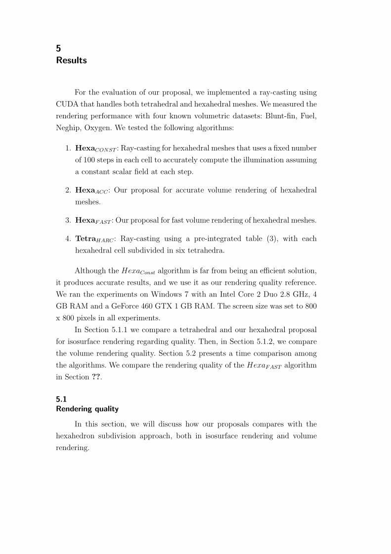
For the evaluation of our proposal, we implemented a ray-casting using

CUDA that handles both tetrahedral and hexahedral meshes. We measured the

rendering performance with four known volumetric datasets: Blunt-fin, Fuel,

Neghip, Oxygen. We tested the following algorithms:

1. HexaCONST : Ray-casting for hexahedral meshes that uses a fixed number

of 100 steps in each cell to accurately compute the illumination assuming

a constant scalar field at each step.

2. HexaACC : Our proposal for accurate volume rendering of hexahedral

meshes.

3. HexaFAST : Our proposal for fast volume rendering of hexahedral meshes.

4. TetraHARC : Ray-casting using a pre-integrated table (3), with each

hexahedral cell subdivided in six tetrahedra.

Although the HexaConst algorithm is far from being an efficient solution,

it produces accurate results, and we use it as our rendering quality reference.

We ran the experiments on Windows 7 with an Intel Core 2 Duo 2.8 GHz, 4

GB RAM and a GeForce 460 GTX 1 GB RAM. The screen size was set to 800

x 800 pixels in all experiments.

In Section 5.1.1 we compare a tetrahedral and our hexahedral proposal

for isosurface rendering regarding quality. Then, in Section 5.1.2, we compare

the volume rendering quality. Section 5.2 presents a time comparison among

the algorithms. We compare the rendering quality of the HexaFAST algorithm

in Section ??.

5.1Rendering quality

In this section, we will discuss how our proposals compares with the

hexahedron subdivision approach, both in isosurface rendering and volume

rendering.

DBD

PUC-Rio - Certificação Digital Nº 0921332/CA

Volume rendering of unstructured hexahedral meshes 28

5.1.1Isosurface rendering

Figure 5.1 compares the isosurface of the Bucky dataset.

As can be noted, our proposal presents smoother isosurfaces, as expected,

since we consider a trilinear scalar function. Both algorithms (HexaACC and

HexaFAST ) presents similar results.

5.1(a): TetraHARC 5.1(b): HexaACC 5.1(c): HexaFAST

Figure 5.1: Bucky dataset isosurfaces.

DBD



5.1.2Volume Rendering Quality

We evaluate our ray-casting algorithms regarding rendering quality. We

first devised an experiment using synthetic volume data composed by only

one hexahedral cell. Figure 5.2 shows the scalar values set to each vertex and

presents the four images achieved by the four algorithms. For these images, we

used a transfer function with six thin spikes, isolating six different slabs. Even

though such a scalar field variation is rare in actual datasets, this synthetic test

aims to show how the subdivision of an hexahedron can lead to unrecognizable

results. The test also demonstrates that both of our proposals are capable of

rendering scalar fields with complex variations.

Figure 5.3 shows and compares the results achieved by the four al-

gorithms for rendering the Bucky model. Figures 5.3(e), 5.3(f) and 5.3(g)

shows the difference between the images achieved with our two proposals and

the subdivision scheme when compared to our quality reference. It’s possible

to notice a clear difference between the rendering images, with our propos-

als more similar to our quality reference. The HexaFAST proposal presents a

subtle difference, expected because of our approximations of the ray integral.

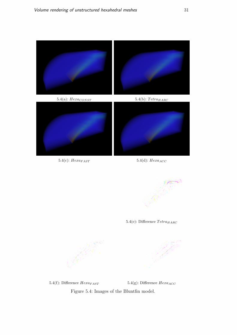
Figure 5.4 shows the result of a similar experiment but now considering

the Bluntfin model. As can be noted, the results are equivalent: our algorithm

produces images with a better quality. In this example, our two proposal

present similar results.

S7=1S5=1

S6=0S4=0

S0=1 S2=0

S1=0 S3=0

y

z

x

5.2(a): Scalar val-ues at vertices

5.2(b):HexaCONST

5.2(c):TetraHARC

5.2(d):HexaFAST

5.2(e): HexaACC

Figure 5.2: Rendering on a synthetic model composed by on hexahedron.

DBD



5.3(a): HexaCONST 5.3(b): TetraHARC

5.3(c): HexaFAST 5.3(d): HexaACC

5.3(e): Difference TetraHARC

5.3(f): Difference HexaFAST 5.3(g): Difference HexaACC

Figure 5.3: Images of the Bucky model.

DBD



5.4(a): HexaCONST 5.4(b): TetraHARC

5.4(c): HexaFAST 5.4(d): HexaACC

5.4(e): Difference TetraHARC

5.4(f): Difference HexaFAST 5.4(g): Difference HexaACC

Figure 5.4: Images of the Bluntfin model.

DBD



5.1.3Comparassion with regular data rendering

We also compared our algorithm with a regular data ray-casting, de-

tailed in Appendix D. Figure 5.5 shows the difference between the different

algorithms. To highlight the differences, we used a transfer function with 100

control points.

As can be seen, our proposal (both using quadrature and linear approx-

imation) presents a better representation of the volume. Due to the trilinear

interpolation during the 3D texture fetch, the rendering of the regular ray-

casting algorithm does not appear as smooth as our proposal. Another prob-

lem is that, even with a 100 steps pre-integrated table, the regular ray-casting

algorithm misses some of the transfer function control points, unlike our pro-

posal, that stops at every control point.

DBD



5.5(a): HexaConst

5.5(b): HexaACC 5.5(c): HexaFAST

5.5(d): Regular ray-casting, using pre-integrated table

5.5(e): Regular ray-casting

Figure 5.5: Achieved images using a synthetic model.

DBD



5.2Time results

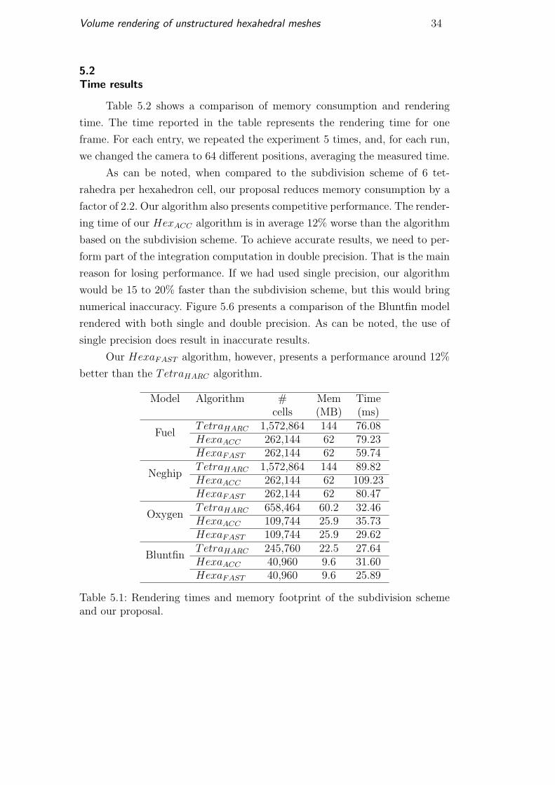
Table 5.2 shows a comparison of memory consumption and rendering

time. The time reported in the table represents the rendering time for one

frame. For each entry, we repeated the experiment 5 times, and, for each run,

we changed the camera to 64 different positions, averaging the measured time.

As can be noted, when compared to the subdivision scheme of 6 tet-

rahedra per hexahedron cell, our proposal reduces memory consumption by a

factor of 2.2. Our algorithm also presents competitive performance. The render-

ing time of our HexACC algorithm is in average 12% worse than the algorithm

based on the subdivision scheme. To achieve accurate results, we need to per-

form part of the integration computation in double precision. That is the main

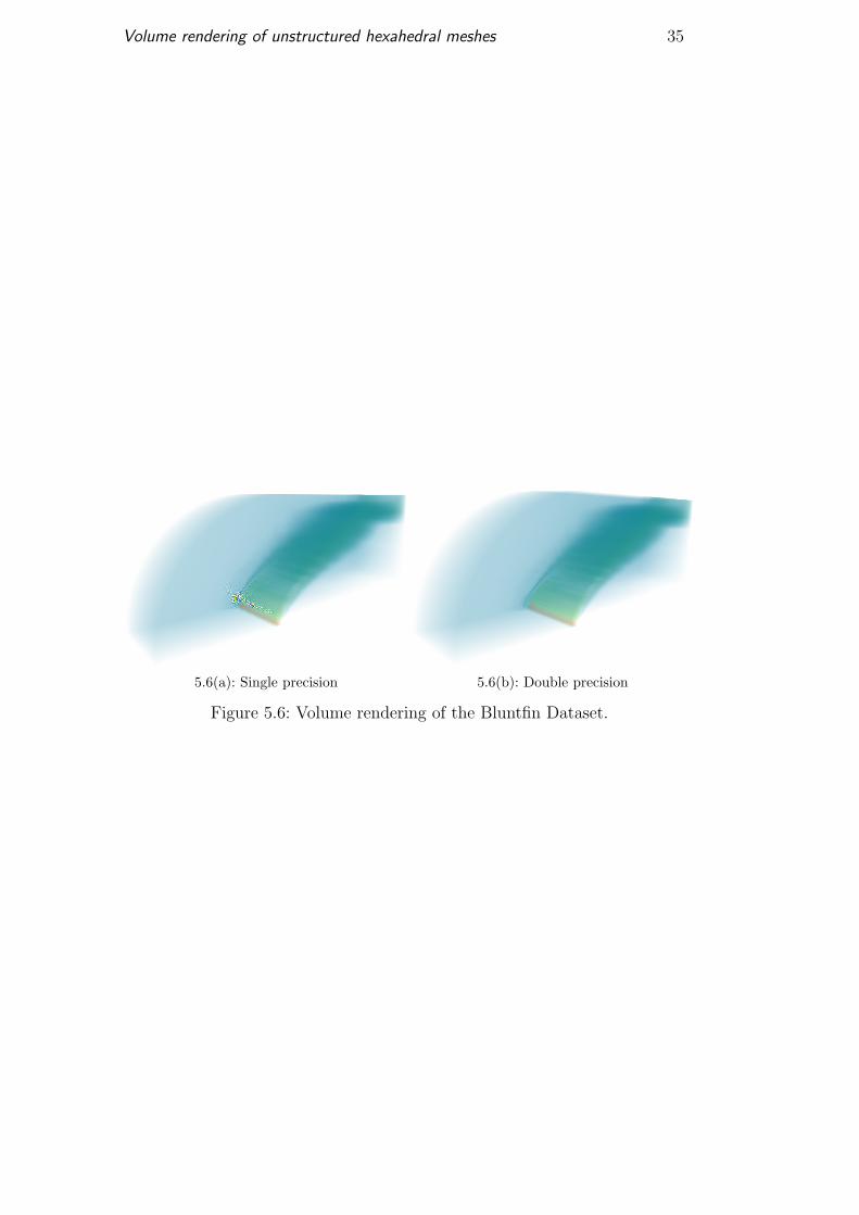
reason for losing performance. If we had used single precision, our algorithm

would be 15 to 20% faster than the subdivision scheme, but this would bring

numerical inaccuracy. Figure 5.6 presents a comparison of the Bluntfin model

rendered with both single and double precision. As can be noted, the use of

single precision does result in inaccurate results.

Our HexaFAST algorithm, however, presents a performance around 12%

better than the TetraHARC algorithm.

Model Algorithm # Mem Timecells (MB) (ms)

FuelTetraHARC 1,572,864 144 76.08HexaACC 262,144 62 79.23HexaFAST 262,144 62 59.74

NeghipTetraHARC 1,572,864 144 89.82HexaACC 262,144 62 109.23HexaFAST 262,144 62 80.47

OxygenTetraHARC 658,464 60.2 32.46HexaACC 109,744 25.9 35.73HexaFAST 109,744 25.9 29.62

BluntfinTetraHARC 245,760 22.5 27.64HexaACC 40,960 9.6 31.60HexaFAST 40,960 9.6 25.89

Table 5.1: Rendering times and memory footprint of the subdivision schemeand our proposal.

DBD



5.6(a): Single precision 5.6(b): Double precision

Figure 5.6: Volume rendering of the Bluntfin Dataset.

DBD


volume rendering of unstructured hexahedral meshes

Documents