financial development, financial fragility, and growth · wp/05/170 financial development,...

WP/05/170

Financial Development, Financial Fragility, and Growth

Norman Loayza and Romain Ranciere

© 2005 International Monetary Fund WP/05/170

IMF Working Paper

Research Department

Financial Development, Financial Fragility, and Growth

Prepared by Norman Loayza and Romain Ranciere1

Authorized for distribution by Paolo Mauro

August 2005

Abstract

This Working Paper should not be reported as representing the views of the IMF. The views expressed in this Working Paper are those of the author(s) and do not necessarily represent those of the IMF or IMF policy. Working Papers describe research in progress by the author(s) and are published to elicit comments and to further debate.

This paper studies the apparent contradictions between two strands of the literature on the effects of financial intermediation on economic activity. On the one hand, the empirical growth literature finds a positive effect of financial depth as measured by, for instance, private domestic credit and liquid liabilities. On the other hand, the banking and currency crisis literature finds that monetary aggregates, such as domestic credit, are among the best predictors of crises and their related economic downturns. This paper accounts for these contrasting effects based on the distinction between the short- and long-run effects of financial intermediation. JEL Classification Numbers: G21, O11, O16 Keywords: Growth empirics, banking crisis, pooled mean group estimation Author(s) E-Mail Address: [email protected]; [email protected]

1 The first draft of this paper was written when both authors were with the Central Bank of Chile. We would like to thank Jason Cummins, Jess Benhabib, and Carlos Vegh for useful comments. Guillermo Vuletin provided excellent research assistance.

- 2 -

Contents Page

I. Introduction .................................................................................................................3 II. Short- and Long-Run Growth Effects of Financial Intermediation ............................5 A. Methodology .........................................................................................................6 B. Data and Results....................................................................................................9 III. Financial Fragility, Alongside Financial Depth, in the Path to Financial Development .......................................................................................................12 A. Theoretical Discussion........................................................................................14 B. Analysis of Short-Run Coefficients ....................................................................15 C. Classical Growth Regressions: The Role of Financial Volatility and Crises......17 D. Data and Methodology........................................................................................20 E. Results ................................................................................................................21 IV. Conclusions...............................................................................................................23 References..........................................................................................................................28 Tables 1. The Long- and Short-Run Effect of Financial Intermediation on Economic Growth ..................................................................................................................10 2. The Long- and Short-Run Effects of Financial Intermediation on Economic Growth, Reduced Sample ......................................................................................13 3. Short-Run Coefficients on Financial Intermediation, Banking Crises, And Financial Volatiliy..........................................................................................16 4. Short-Run Effects of Financial Intermediation Depending on Presence of Banking Crises and Volatility................................................................................18 5. The Growth Effect of Financial Depth, Financial Volatility, and Financial Crises......................................................................................................................22 Figures 1. Economic Growth and Financial Intermediation Around Banking Crises .................4 2. Economic Growth and Financial Intermediation in the Long Run.............................4 3. Frequency Distribution of Short-Run Coefficients for Various Groupings..............19 Appendices I. Sample of Countries .................................................................................................24 II. Definitions and Sources of Variables Used in Regression Analysis........................26 III. Descriptive Statistics.................................................................................................27

- 3 -

I. INTRODUCTION

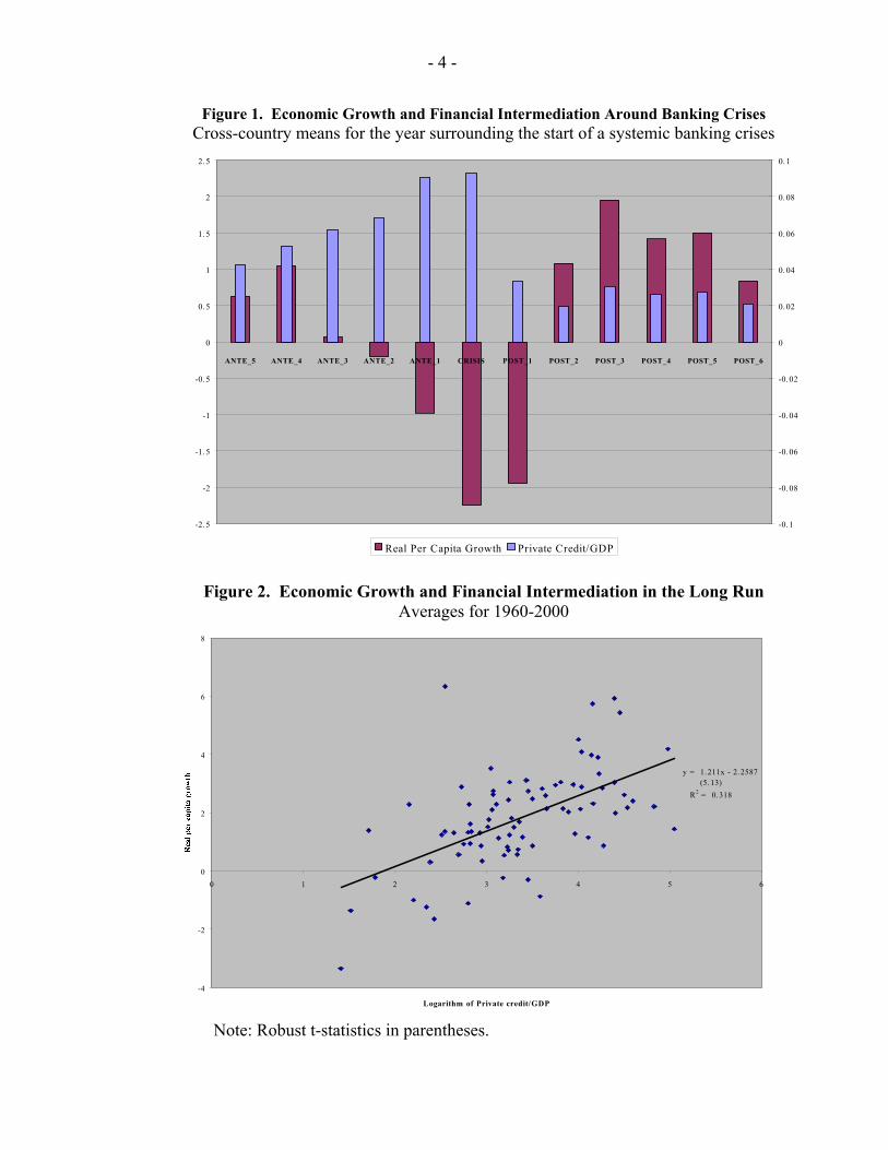
This paper analyzes the apparent contradiction between two strands of the literature on the effects of financial intermediation on economic activity. On the one hand, the empirical growth literature finds a positive effect of measures of private domestic credit and liquid liabilities on per capita GDP growth (see Figure 1). This is interpreted as the growth enhancing effect of financial development (e.g., King and Levine, 1993; Levine, Loayza, and Beck, 2000). On the other hand, the banking and currency crisis literature finds that monetary aggregates, such as domestic credit, are among the best predictors for crises (e.g., Demirguc-Kunt and Detragiache 1998 and 2000; Gourinchas, Landerretche, and Valdés, 2001; Kaminsky and Reinhart, 1999). Since banking crises usually lead to recessions, an expansion of domestic credit would then be associated with growth slowdowns (see Figure 2).

A similar divide exists at the theoretical level. According to the endogenous growth literature, financial deepening leads to a more efficient allocation of savings to productive investment projects (see Greenwood and Jovanovic, 1990; Bencivenga and Smith, 1991). Conversely, the financial crisis literature points to the destabilizing effect of financial liberalization as it may lead to an unduly large expansion of credit. Overlending may occur owing to a number of factors, including a limited monitoring capacity of regulatory agencies, the inability of banks to discriminate good projects during investment booms, and the existence of an explicit or implicit insurance against banking failures (Schneider and Tornell, 2004; Aghion, Bacchetta and Banerjee, forthcoming). Not surprisingly, each strand of the literature has produced its own set of policy implications. Thus, researchers who emphasize the findings of the endogenous growth literature advocate financial liberalization and deepening (e.g., Roubini and Sala-i-Martin, 1992), whereas those who concentrate on crises caution against “excessive” financial liberalization (e.g., Balino and Sundarajan, 1991; Gavin and Hausmann, 1995).

This paper contributes to the debate on the effects of financial deepening from an empirical perspective. First, we highlight the contrasting effects of financial liberalization and credit expansion on economic activity. Second, we attempt to provide an empirical explanation for these contrasting effects. In particular, on the one hand, we relate the positive influence of financial depth on investment and growth to the long-run effect of financial liberalization; but, on the other, we identify a link between the negative impact of financial volatility and crisis and the short-run effect of liberalization. Although it is not our aim to test competing theories, our empirical results provide support to some recent theoretical models predicting that financial liberalization can generate both short-run instability and higher long-run growth.

- 4 -

Figure 1. Economic Growth and Financial Intermediation Around Banking Crises Cross-country means for the year surrounding the start of a systemic banking crises

-2.5

-2

-1.5

-1

-0.5

0

0.5

1

1.5

2

2.5

ANTE_5 ANTE_4 ANTE_3 ANTE_2 ANTE_1 CRISIS POST_1 POST_2 POST_3 POST_4 POST_5 POST_6

-0.1

-0.08

-0.06

-0.04

-0.02

0

0.02

0.04

0.06

0.08

0.1

Real Per Capita Growth Private Credit/GDP

Figure 2. Economic Growth and Financial Intermediation in the Long Run Averages for 1960-2000

y = 1.211x - 2.2587(5.13)

R2 = 0.318

-4

-2

0

2

4

6

8

0 1 2 3 4 5 6

Logarithm of Private credit/GDP

Note: Robust t-statistics in parentheses.

- 5 -

The paper is organized as follows. In Section II we examine the output growth effects of cyclical and trend changes of financial intermediation. We estimate a model that incorporates both short- and long-run effects using a panel of cross-country and time-series observations. Our basic econometric technique is the Pooled Mean Group estimator developed by Pesaran, Shin, and Smith (1999). By focusing on effects at different time horizons, we set the basis for an explanation of the apparently contradictory effects of financial intermediation on economic activity. In Section III, we further develop this explanation. First, we link our short- and long-run results to recent theoretical models on the effects of financial liberalization. Second, since our econometric methodology allows us to estimate country-specific short-run effects of financial intermediation on output growth, we analyze their relationship with country-specific measures of financial fragility, namely, banking crises and volatility. And third, we return to the classic context of growth regressions and consider whether the volatility and crises aspects of financial liberalization are relevant growth determinants, along with the usual measures of financial depth. Finally, Section IV concludes.

II. SHORT- AND LONG-RUN GROWTH EFFECTS OF FINANCIAL INTERMEDIATION

In this section, we estimate an empirical model that encompasses the short- and long-run growth effects of financial intermediation. We use the estimation results to formulate an empirical explanation of the apparently contradictory effects of financial intermediation on economic activity. This explanation is based on the distinction between the cycle and trend changes of financial intermediation and their corresponding effects on output growth.

Instead of averaging the data per country to isolate trend effects, we estimate both short- and long-run effects using a data field composed of a relatively large sample of countries and annual observations. Our method can be summarized as a panel error-correction model, where short- and long-run effects are estimated jointly from a general autoregressive distributed-lag (ARDL) model and where short-run effects are allowed to vary across countries.

We propose this panel error-correction method as an alternative to the traditional method of time averaging for the following reasons. First, while averaging clearly induces a loss of information, it is not obvious that averaging over fixed-length intervals effectively eliminates business-cycle fluctuations. Second, averaging eliminates information that may be used to estimate a more flexible model that allows for some parameter heterogeneity across countries. Third, and most importantly for our purposes, averaging hides the dynamic relationship between financial intermediation and economic activity, particularly the presence of opposite effects at different time frequencies.2

2 Similar arguments are made by Attanasio, Picci, and Scorcu (2000) in their cross-country study on the dynamic relationship between saving, investment, and growth.

- 6 -

A. Methodology

Empirical estimation poses two issues. The first is the need to separate and estimate short- and long-run effects without the need to decompose directly trend and transitory components of growth, financial intermediation, and the other explanatory variables. We treat this issue below in the context of single-country estimation. The second issue is the likely possibility that the parameters in the relationship between financial intermediation and economic activity be different across countries. It can be argued that country heterogeneity is particularly relevant in short-run relationships, given that countries are affected by overlending and financial crises to widely different degrees. On the other hand, we can expect that long-run relationships would be more homogeneous across countries. We discuss below the issue of heterogeneity in the context of multi-country estimation.

Single-Country Estimation The challenge we face is to estimate long- and short-run relationships without observing the long- and short-run components of the variables involved. Over the last decade or so, a booming cointegration literature has focused on the estimation of long-run relationships among I(1) variables (Johansen 1995, Phillips and Hansen 1990). From this literature, two common misconceptions have been derived. The first one is that long-run relationships exist only in the context of cointegration among integrated variables. The second one is that standard methods of estimation and inference are incorrect.

A recent literature, represented in Pesaran and Smith (1995), Pesaran (1997) and Pesaran and Shin (1999), has argued against both misconceptions. These authors show that simple modifications to standard methods can render consistent and efficient estimates of the parameters in a long-run relationship between both integrated and stationary variables and that inference on these parameters can be conducted using standard tests. Furthermore, these methods avoid the need for pre-testing and order-of-integration conformability given that they are valid whether the variables of interest are I(0) or I(1). The main requirements for the validity of this methodology are that, first, there exist a long-run relationship among the variables of interest and, second, the dynamic specification of the model be sufficiently augmented so that the regressors are strictly exogenous and the resulting residuals are serially uncorrelated.3 Pesaran and co-authors label this the “autoregressive distributed lag (ARDL) approach” to long-run modeling.

In order to comply with the requirements for standard estimation and inference, we embed a long-run growth regression equation into an ARDL (p, q) model. In error-correction form, this can be written as follows:

3 It is worth noting that the assumption of a unique long-run relationship underlies implicitly the various single-equation based estimators of long-run relationships commonly found in the cointegration literature. Without such assumption, these estimators would at best identify some linear combination of all the long-run relationships present in the data.

- 7 -

( ) ( ) ( ) ( ) ( ){ }[ ] ittiii

tii

q

jjti

ijjti

p

j

ijti XyXyy εββϕδγ ++−+∆+∆=∆ −−

−

=−−

−

=∑∑ 1101

1

0

1

1 (1)

where y is the per capita GDP growth rate, X represents a set of growth determinants including financial depth and control variables, γ and δ are the short-run coefficients related to growth and its determinants, β are the long-run coefficients, ϕ is the speed of adjustment to the long-run relationship, ε is a time-varying disturbance, and the subscripts i and t represent country and time, respectively. The term in square brackets contains the long-run growth regression, which acts as a forcing equilibrium condition:

( ) ( ) )0(~ e wher ,,10 IXy tititiii

ti µµββ ++= (2)

Multi-Country Estimation The sample we use for estimation is a “data field,” in the sense that it is characterized by time-series (T) and cross-section (N) dimensions of roughly similar magnitude. In such conditions, there are a number of alternative methods for multi-country estimation that vary in the extent to which they allow for parameter heterogeneity across countries. At one extreme, the fully heterogeneous-coefficient model imposes no cross-country parameter restrictions and can be estimated on a country-by-country basis—provided the time-series dimension of the data is sufficiently large. When, in addition, the cross-country dimension is also large, the mean of long- and short-run coefficients across countries can be estimated consistently by the unweighted average of the individual country coefficients. This is the mean group (MG) estimator introduced by Pesaran, Smith, and Im (1996). At the other extreme, the fully homogeneous-coefficient model requires that all slope and intercept coefficients be equal across countries. This is the simple pooled estimator.

In between the two extremes, there is a variety of estimators. The dynamic fixed effects estimator restricts all slope coefficients to be equal across countries but allows for different country intercepts. The pooled mean group (PMG) estimator, introduced by Pesaran, Shin and Smith (1999), restricts the long-run slope coefficients to be the same across countries but allows the short-run coefficients (including the speed of adjustment) and the regression intercept to be country specific. The PMG estimator also generates consistent estimates of the mean of short-run coefficients across countries by taking the simple average of individual country coefficients (provided that the cross-sectional dimension is large).

The choice among these estimators faces a general trade-off between consistency and efficiency. Estimators that impose cross-country constraints dominate the heterogeneous estimators in terms of efficiency if the restrictions are valid. If they are false, however, the restricted estimators are inconsistent. In particular, imposing invalid parameter homogeneity in dynamic models typically leads to downward-biased estimates of the speed of adjustment (Robertson and Symons, 1992; Pesaran and Smith, 1995).

- 8 -

For our purposes, the pooled mean group estimator offers the best available compromise in the search for consistency and efficiency. This estimator is particularly useful when the long run is given by conditions expected to be homogeneous across countries while the short-run adjustment depends on country characteristics such as vulnerability to domestic and external shocks, monetary and fiscal adjustment mechanisms, financial-market imperfections, and relative price and wage flexibility. Furthermore, the PMG estimator is sufficiently flexible to allow for long-run coefficient homogeneity over only a subset of variables and/or countries.

Therefore, we use the PMG method to estimate a long-run relationship that is common across countries (i.,e, β1

i = β1

j for all countries i, j) while allowing for unrestricted country

heterogeneity in the adjustment dynamics and fixed effects. The interested reader is referred to Pesaran, Shin and Smith (1999), where the PMG estimator is developed and compared with the MG estimator. Briefly, the PMG estimator proceeds as follows. First, the estimation of the long-run slope coefficients is done jointly across countries through a (concentrated) maximum likelihood procedure. Second, the estimation of short-run coefficients (including the speed of adjustment ϕi), country-specific intercepts β0

i, and country-specific error variances is done on a country-by-country basis, also through maximum likelihood and using the estimates of the long-run slope coefficients previously obtained.4

An important assumption for the consistency of the PMG estimates is the independence of the regression residuals across countries. In practice, non-zero error covariances usually arise from omitted common factors that influence the countries’ ARDL processes. We attempt to eliminate these common factors and, thus, ensure the independence condition by allowing for time-specific effects in the estimated regression; this is equivalent to a regression in which each variable enters as deviations with respect to the cross-sectional mean in a particular year.

As indicated in the previous section, for each country the order of the ARDL process must be augmented to ensure that the residual of the error-correction model be exogenous and serially

4 The comparison of the asymptotic properties of PMG and MG estimates can be put also in terms of the general trade-off between consistency and efficiency noted in the text. If the long-run coefficients are in fact equal across countries, then the PMG estimates will be consistent and efficient, whereas the MG estimates will only be consistent. If, on the other hand, the long-run coefficients are not equal across countries, then the PMG estimates will be inconsistent, whereas the MG estimator will still provide a consistent estimate of the mean of long-run coefficients across countries. The long-run homogeneity restrictions can be tested using Hausman or likelihood ratio tests to compare the PMG and MG estimates of the long- run coefficients. In turn, comparison of the small sample properties of these estimators relies on their sensitivity to outliers. In small samples (low T and N), the MG estimator, being an unweighted average, is very sensitive to outlying country estimates (for instance those obtained with small T). The PMG estimator performs better in this regard because it produces estimates that are similar to weighted averages of the respective country-specific estimates, where the weights are given according to their precision (that is, the inverse of their corresponding variance-covariance matrix).

- 9 -

uncorrelated. At the same time, with a limited number of time-series observations, the ARDL order should not be overextended as this imposes excessive parameter requirements on the data. When the main interest is on the long-run parameters, the lag order of the ARDL can be selected using some consistent information criteria (such as the Schwartz-Bayesian Criterion) on a country-by-country basis. However, when there is also interest in analyzing and comparing the short-run parameters, it is recommended to impose a common lag structure across countries, in accordance to the characteristics of the analytical model to be studied and the limitations of the data. We use the latter approach in this paper’s implementation of the ARDL approach.

B. Data and Results

The sample consists of 75 countries with annual data during the period 1960-2000. See Appendix 1 for the list of countries included in the sample. Given the procedure’s requirements on the time-series dimension of the data, we include only countries that have at least 20 consecutive observations. The dependent variable is the growth rate of GDP per capita. The measure of financial intermediation is private domestic credit as ratio to GDP.5 The control variables are the initial level of GDP per capita, government consumption as ratio to GDP, structure-adjusted trade openness,6 and the inflation rate. In order to capture proportional effects, all control variables are specified in natural logs. See Appendix II for definitions and sources of all variables used in the paper, and Appendix III for their descriptive statistics. Table 1 presents the results on specification tests and the estimation of long- and short-run parameters linking per capita GDP growth, financial intermediation, and other growth determinants. We emphasize the results obtained using the pooled mean group (PMG) estimator, which we prefer given its gains in consistency and efficiency over other panel error-correction estimators. For comparison purposes, we also present the results obtained with the mean group (MG) and the dynamic fixed-effects (DFE) estimators. As outlined in the previous section, the consistency and efficiency of the PMG estimates relies on several specification conditions. The first is that the regression residuals be serially uncorrelated and that the explanatory variables can be treated as exogenous. We seek to fulfill these conditions by including in the ARDL model, 3 lags of the growth rate, 3 lags of the measure of finance intermediation, and 1 lag of each control variable. We

5 The other popular measure of financial intermediation is the ratio of liquid liabilities to GDP. As a robustness check, we have repeated all empirical exercises presented in the paper substituting liquid liabilities for private credit. Since these results are essentially the same as those using private credit/GDP, we have omitted them in this version of the paper but can make them available upon request. 6 Trade openness is the residual of a regression of the log of the ratio of exports (in 1995 U.S. dollar) to GDP (in 1995 U.S. dollar), on the logs of area and population, and dummies for oil exporting and for landlocked countries.

- 10 -

Variables Coef. St.Er. Coef. St.Er. h-test p-val Coef. St.Er.Long-Run CoefficientsFinancial intermediation 0.708 0.179 0.948 1.226 0.04 0.84 0.121 0.473Initial GDP per capita -8.609 0.571 -13.803 4.52 1.34 0.25 -3.489 0.488Government size -5.705 0.463 -9.217 4.122 0.48 0.49 -2.022 0.462Trade openness 1.059 0.281 5.176 2.199 4.56 0.03 1.504 0.340Inflation -5.969 0.684 4.335 5.899 0.08 0.78 -4.979 0.767

Joint Hausman Test: 8.5 0.13

Error Correction CoefficientsPhi -0.973 0.063 -2.36 0.156 -0.943 0.034

Short-Run Coefficients ∆ Growth (-1) 0.178 0.056 1.003 0.121 0.041 0.027∆ Growth (-2) 0.02 0.035 0.447 0.07 -0.017 0.020∆ Financial intemediation -4.517 1.136 -2.814 2.008 -10.258 2.137∆ Financial intermediation (-1) -0.591 1.028 -0.087 1.662 4.930 2.328∆ Financial intermediation (-2) -0.856 1.310 0.486 1.617 -5.570 2.262∆ Initial GDP per capita -4.954 2.947 -9.019 5.052 -5.142 1.919∆ Government size -0.08 1.751 3.76 2.288 -2.894 0.738∆ Trade openness 3.344 2.223 -4.294 3.626 2.127 0.752∆ Inflation -2.258 1.842 -0.782 5.046 -0.674 0.871Intercept -1.24 2.273 -10.121 13.104 -0.010 0.007

Sum of Coefficients on Financial Intermediation Σ∆ Financial intemediation coeffs. -5.964 2.316 -2.415 4.24

No. Countries 75 75 75No. Observations 2501 2501 2501Avg. Rbar squared 0.454 0.67 0.484

Source: Authors' estimates

Pooled Mean Group Mean Group Hausman Tests Dynamic Fixed Effect

Table 1. The Long- and Short-Run Effect of Financial Intermediation on Economic Growth Estimators: Pooled Mean Group, Mean Group, and Dynamic Fixed Efffects, All Controlling for Country and Time Effects

Dynamic Specification: ARDL (3, 3, 1, 1, 1, 1)Sample: All Countries, Annual Data 1960-2000

- 11 -

could not expand the lag structure any further because we would run into problems of lack of degrees of freedom. We chose to use a richer (longer) lag structure for the dependent variable (growth) and the variable of interest (financial intermediation) because our main concern was to characterize their long- and short-run relationships.

The second specification condition is that both country-specific effects and cross-country common factors be accounted for. We control for country-specific effects by allowing for an intercept for each country, and we attempt to eliminate cross-country common factors by demeaning the data using the corresponding cross-sectional means for every period (which is algebraically the same as allowing for year-specific intercepts). The third condition refers to the existence of a long-run relationship (dynamic stability) and requires that the coefficient on the error-correction term be negative and not lower than -2 (that is, within the unit circle). In the second panel of Table 1, we report the estimates for the pooled error-correction coefficient and its corresponding standard error. This coefficient falls within the dynamically stable range in the cases of the PMG and dynamic fixed effects estimators. The fact that the pooled error correction coefficient falls outside the allowed range in the case of the mean group estimator reveals that for some countries the dynamic stability condition does not hold. We come back to this issue below.

The fourth condition is that the long-run parameters be the same across countries. As explained in the section on econometric methodology, we can test the null hypothesis of homogeneity through a Hausman-type test, based on the comparison between the Pooled Mean Group and the Mean Group estimators. In Table 1 we present the Hausman test statistic and the corresponding p-values for the coefficients on each of the explanatory variables and for all of them jointly. The homogeneity restriction is not rejected jointly for all parameters; it is not rejected for individual parameters either except in the case of trade openness.

Regarding the estimated parameters, our analysis focuses on those obtained with the PMG estimator. In the long run, the growth rate of GDP per capita is negatively related to initial income, the size of government, and the inflation rate, and positively related to international trade openness. These are standard results from the empirical growth literature, and it is reassuring that we are able to reproduce them with our methodology.

Most importantly for our purposes, we find that economic growth is positively and significantly linked to the measure of financial intermediation in the long run. This effect is also economically significant--the estimated coefficient implies that if a country deepens its financial market so as to move from the 25th to the 50th percentile of the world distribution of private credit/GDP (from 15.4% to 26%), it will increase its per capita GDP growth rate by 1.45 percentage points.

The short-run coefficients on financial intermediation tell a different story. As explained earlier, short-run coefficients are not restricted to be the same across countries, so that we do not have a single pooled estimate for each coefficient. Nevertheless, we can still analyze the average short-run effect by considering the mean of the corresponding coefficients across

- 12 -

countries. We find that the short-run average relationship between the growth rate of GDP per capita and the measure of financial intermediation appears to be strongly negative, with a point estimate several times larger than that of the long-run effect of financial intermediation. Thus, comparing the long- and short-run estimates, a first broad conclusion is that the sign of the relationship between economic growth and financial intermediation depends on whether their movements are temporary or permanent.

In the next section we will take advantage of the cross-country variation of short-run coefficients to draw a connection between the negative effects of financial intermediation and the occurrence of financial volatility and crisis. Before we do that, however, we need to make sure that our results are robust to the exclusion of outlying and dynamically unstable observations. In particular, we want to check to what extent the long-run coefficients and especially the average of short-run coefficients are sensitive to the exclusion of countries whose estimated short-run effects are considerably larger (in absolute value) than typical effects in the sample and countries that present error-correction coefficients that statistically fall outside the dynamic stable range. We exclude the countries whose short-run coefficients fall outside 2 standard deviations from the mean: Dominican Republic, Ghana, Sierra Leone, Thailand, Turkey, and Democratic Republic of Congo. We also exclude the countries for which the estimates do not meet the econometric condition of dynamic stability.

The results on the restricted sample are presented in Table 2. They are qualitatively similar to those on the full sample. The signs and statistical significance of all long-run and most short-run coefficients remain unchanged. The Hausman test does not reject the joint homogeneity of all long-run parameters; and it does not reject the homogeneity of individual long-run coefficients except for that on initial income. Moreover, the long- and short-run effects of private credit on growth are not only qualitatively but also quantitatively very similar for the restricted and full samples.

III. FINANCIAL FRAGILITY, ALONGSIDE FINANCIAL DEPTH,

IN THE PATH TO FINANCIAL DEVELOPMENT

By focusing on the effects of financial intermediation at different time horizons, the analysis conducted in the previous section helps us set the basis for an explanation of the apparently contradictory effects of financial intermediation on economic activity. In this section, we discuss and develop further this explanation. First, we review a selected set of recent theoretical models that examine the evolution of the effects of financial liberalization through time. All of them differentiate between short- and long-run effects on economic growth. Moreover, they highlight the point that financial liberalization is not only associated with financial depth but also to financial fragility (as captured by banking crises and financial volatility), and it is this aspect of financial liberalization that explains why intermediation may have a negative short-run effect on growth. Second, we consider this possibility by examining the connection between country-specific measures of financial volatility and crisis

- 13 -

Pooled Mean Group Mean Group Hausman Tests Dynamic Fixed Effect

Variables Coef. St.Er. Coef. St.Er. h-test p-val Coef. St.Er.

Long-Run CoefficientsFinancial intermediation 0.632 0.259 0.165 1.314 0.06 0.81 0.107 0.260Initial GDP per capita -5.181 0.513 -13.886 3.893 5.09 0.02 -3.423 0.512Government size -2.342 0.41 -1.53 4.06 0.04 0.84 -2.022 0.462Trade openness 2.422 0.188 2.871 3.133 0.03 0.89 1.458 0.352Inflation -5.029 0.596 -4.568 5.849 0.01 0.94 -5.162 0.771

Joint Hausman Test: 7.72 0.17

Error Correction CoefficientsPhi -0.901 0.069 -1.867 0.118 -0.916 0.035

Short-Run Coefficients ∆ Growth (-1) 0.144 0.049 0.739 0.091 0.056 0.028∆ Growth (-2) 0.001 0.031 0.314 0.053 -0.003 0.021∆ Financial intemediation -5.056 1.033 -4.571 1.762 -2.453 0.591∆ Financial intermediation (-1) -0.113 1.090 -1.027 1.675 -0.079 0.591∆ Financial intermediation (-2) -0.534 1.029 -0.64 1.434 -0.346 0.594∆ Initial GDP per capita -6.115 2.613 -7.511 4.192 -4.712 2.007∆ Government size -6.509 2.171 -7.14 3.525 -3.192 0.751∆ Trade openness 3.358 2.18 -2.819 2.719 2.660 0.816∆ Inflation -4.789 1.576 4.752 4.14 -1.873 0.901Intercept -0.881 1.312 -7.696 10.063 -0.004 0.007

Sum of Coefficients on Financial Intermediation Σ∆ Financial intemediation coeffs. -5.702 1.628 -6.238 4.31

No. Countries 66 66 66No. Observations 2206 2206 2206Avg. Rbar squared 0.449 0.65 0.47

Source: Authors' estimates

Table 2. The Long- and Short-Run Effects of Financial Intermediation on Economic Growth, Reduced Sample Estimators: Pooled Mean Group, Mean Group, and Dynamic Fixed Efffects, All Controlling for Country and Time Effects

Dynamic Specification: ARDL (3, 3, 1, 1, 1, 1)Sample: Countries That are not Ouliers or Dynamically Unstable (66 Countries), Annual Data 1960-2000

- 14 -

frequency and the country-specific short-run effects of financial intermediation estimated in the previous section. Finally, as a further test of the relevance of our results, we take the usual approach of empirical growth analysis in order to consider whether the volatility and crisis aspects of financial liberalization, and not only the customary measures of financial depth, are significant determinants of economic growth.

A. Theoretical Discussion

How can we explain the contrast between the short- and long-run effects of financial intermediation? Recent theories on the aftermath of financial liberalization can provide some guidance to answer this question. We do not attempt to tell them apart by testing their particular implications; rather, we intend to draw on their similarities to build a sensible explanation. Gaytán and Rancière (2003) develop a model of banking development where banks serve the purpose of providing liquidity insurance — which avoids the need for costly asset liquidation — but are subject to confidence crises leading to bank runs. Banks have the option to insure against these crises, but this is costly as it entails less money available for investment. Gaytán and Ranciere find that in emerging market countries it is optimal for banks to be only partially covered against the risk of bank runs. This is so because in these countries the opportunity cost of full insurance, given by the marginal rate of return to investment, is too high. As countries develop and capital productivity decreases, it becomes optimal for banks to be fully covered against crises. Therefore, the model predicts that in the short run after financial liberalization, there is the chance that emerging market countries will face financial crises, switch from non-crisis to crisis equilibria, and thus experience volatility of credit and low output growth. In the long run, however, financial development would foster stable growth.

Dell’Ariccia and Marquez (2004a, 2004b) view the aftermath of financial liberalization as a period marked by excessive lending, as banks’ screening incentives are not at par with the rapid growth of credit demand. In their model, banks’ incentives to screen potential borrowers come from adverse selection among banks: in fact, banks screen to avoid financing firms whose projects have been tested and rejected by other banks. When financial markets are liberalized and many new and untested projects request funding, banks do not have strong incentives to screen their pool of applicants and rapid credit expansion ensues. In this case the quality of banks’ portfolio is likely to deteriorate and over-lending will result in financial fragility. At the macroeconomic level, as negative shocks occur, financial fragility will give way to financial instability and output losses. Over time, however, as most potential borrowers are tested, banks’ screening incentives and practices are restored, and lending begins to grow at stable rates. Then, whereas the short run of financial liberalization is marked with financial crisis, volatility, and low output growth, in the long run financial liberalization is bound to improve economic growth. Rajan (1994) develops a similar mechanism that focuses on bankers’ incentives to explain financial fragility. In his model, bank managers tend to hide non-performing loans by maintaining liberal credit policies when most borrowers are solvent (“good” times). When the economy is hit by an aggregate shock and the relative ability of individual managers becomes less discernible, they have the incentive to tighten credit policy. This procyclical credit practice tends to finance bad projects in good times and squeeze credit away from

- 15 -

worthy firms in distress times. The way to solve this inefficient credit practice is through proper banking supervision. However, in the short run after financial liberalization, a great need for credit expansion occurs in the face of poor development of supervisory capacity. In this context, cycles of booms and busts in credit and output growth are likely to arise, and they are only gradually replaced by stable financial depth and output growth as institutional and supervisory capacities develop. Wynne (2002) argues that the fundamental problem underlying financial fragility does not reside in banks’ incentives to screen and monitor potential borrowers; rather, the problem is that it takes time and effort for firms to build financial reputation and public knowledge about the quality of their investment projects. This is important because of the intrinsic asymmetry of information between potential borrowers and creditors. Firms create “information” capital only gradually through a higher survival rate and wealth accumulation. When financial liberalization occurs and a large cohort of new firms enters the market, the absence of information capital leads to high interest rates, risky banks’ loan portfolios, and credit misallocation. At the macroeconomic level, this may result in banking crises, cycles of credit expansion and contraction, and low output growth, particularly if the economy is hit by large shocks. Over time, however, good firms build information capital, lending rates decrease, and banks’ loan portfolios become safer. At the aggregate level, in the long run proper credit allocation results in higher and more stable productivity growth.

All these models predict a positive long-run relationship between financial intermediation and economic growth. They also predict that in the short run this relationship may be negative, and explain through what channels this might occur. What these explanations have in common is that they all link the potential negative short-run impact of financial intermediation with the presence of financial volatility and the likelihood of banking crises. Given that our panel data methodology allows us to recover country-specific short-run coefficients, we can analyze their connection with financial volatility and crises, and to this we turn next.

B. Analysis of Short-Run Coefficients

We consider the question of whether the negative short-run relationship between growth and financial intermediation can be linked to the occurrence of systemic banking crisis and financial volatility. We quantify this short-run relationship by the short-run coefficients on financial intermediation estimated previously for each country in the sample. As a proxy for financial crises, we use the number of years in the period 1960-2000 that the country has experienced systemic banking crises, according to Caprio and Klingebiel (2003). We measure financial volatility as the standard deviation of the growth rate of the private credit to GDP ratio over the period 1960-2000.

Table 3 reports the simple and rank correlation coefficients--along with the corresponding p-values--between the short-run coefficients and the measures of financial crisis and financial volatility. We present statistics corresponding to both the full and restricted samples. Not surprisingly, the correlation between crises and volatility is positive and significant, with values between 0.35 and 0.40. This is large enough to reveal a meaningful connection but sufficiently small to indicate that each variable contains independently relevant information.

- 16 -

(a) Sample: All Countries, Average 1960-2000

Short-run coefficients Number of crises Financial volatility-0.303 -0.379(0.008) (0.001)

-0.2693 0.449(0.0195) (0.000)-0.2980 0.3947(0.0094) (0.0005)

(b) Sample: 66 Countries, Average 1960-2000

Short-run coefficients Number of crises Financial volatility-0.243 -0.345(0.049) (0.005)

-0.2740 0.366(0.0260) (0.002)-0.3153 0.3565(0.0099) (0.0033)

Note: p-values reported in parentheses.Source: Authors' estimates

Number of crises

Financial volatility

1

1

Short-run coefficients

Number of crises

Financial volatility


1

1

1

1

Standard Correlation Coefficients in Upper Rigth Triangular Matrix Spearman Rank Correlation Coefficients in Lower Left Triangular Matrix

Table 3. Short-Run Coefficients on Financial Intermediation, Banking Crises, and Financial Volatility

- 17 -

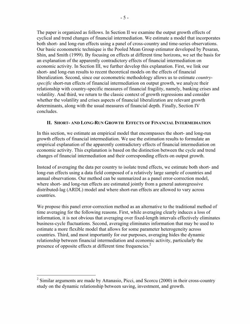
Most importantly, both financial crises and volatility have a negative and significant correlation (close to -0.30) with the estimated short-run coefficients; that is, larger volatility or higher frequency of crises are related to more negative short-run impacts of financial intermediation on output growth. Another approach to examine this connection is by dividing the sample of countries according to criteria given by financial crises and volatility and then comparing the corresponding group means of short-run coefficients. Regarding financial crises, we divide the sample, first, according to whether countries had any crises during the 40 year period (about 60% had at least one year of crisis), and, second, according to whether they are above or below the median number of crises. Regarding financial volatility, we divide the sample using as thresholds, first, the 75th percentile of volatility and, second, its median value. Table 4 presents the tests of the difference in short-run coefficient means for the various ways of grouping countries. We do so for both the full and restricted samples. Countries that experienced financial crises in the last 40 years exhibit an average short-run impact of financial intermediation on output growth that is significantly more negative than the average of countries that did not have any crisis. In fact, for the non-crisis countries, the average short-run impact of intermediation on growth is statistically zero. A similar result is obtained when we divide the sample according to the median frequency of crises: high-crisis countries show significantly more negative short-run impacts than low-crisis countries, and for the latter this impact is indistinguishable from zero. Concerning financial volatility, when we divide the sample using its 75th percentile as threshold, we find that the group of high financial volatility has an average short-run effect that is significantly more negative than the group of low and medium volatility. The results are similar when we use the median volatility as threshold, but in this case the difference in the average short-run coefficients between the two groups is not statistically significant at conventional levels. Figure 3 (a) presents the (smoothed) frequency distributions of short-run coefficients for the groups of crisis and non-crisis countries. Figure 3 (b) does the same for the groups of high-volatility and medium-to-low-volatility countries (using the 75th percentile as threshold). In both cases we consider only the restricted sample of countries (that is, without outliers and dynamically unstable observations). The distributions appear to be basically symmetrical. We can see that the groups of crisis and high-volatility countries not only have more negative average short-run coefficients but also have more dispersed distributions, with fatter tails particularly towards the negative portion of the spectrum.

C. Classical Growth Regressions: The Role of Financial Volatility and Crises

So far our analysis has used a novel empirical estimator to distinguish between short- and long-run effects of financial intermediation on economic growth. This methodology uses the time-series dimension of the data at least as intensively as the cross-country dimension. It represents a departure from the typical empirical growth literature in which high-frequency movements in the data are averaged out prior to estimation. Typical panel-data growth studies work with country data averaged for periods of 5 or 10 years and, therefore, are likely to combine short- and long-run effects. In previous sections of the paper, we have argued that the contrasting effects of financial intermediation come from different aspects associated to

- 18 -

Table 4. Short-Run Effects of Financial Intermediation Depending on Presence of Banking Crises and Volatility

(a) No Crisis Vs. Some Crisis

Mean short-run coefficients

Std. error N° obs. Mean short-run coefficients

Std. error N° obs.

No Crisis -0.199 2.58 30 -1.093 1.77 29 Some Crisis -9.808 3.36 45 -9.315 2.49 37

Test of difference in means:Ho: mean(no crisis) - mean(some crisis) = diff = 0 vs. Ha: diff > 0

diff t-value p-value diff t-value p-value9.609 2.27 0.013 8.222 2.69 0.005

(b) Low Crisis Vs. High Crisis



Std. error N° obs.

Low crisis -0.343 2.33 34 -1.472 1.62 32 High crisis -10.626 3.64 41 -9.684 2.7 34

Test of difference in means: Ho: mean(crisis below median) - mean(crisis above median) = diff = 0 vs. Ha: diff > 0


(c) Low and Medium Financial Volatility Vs. High Financial Volatility



Std. error N° obs.

Low and medium volatility -3.064 2.53 56 -4.227 1.91 51 High volatility -14.515 4.92 19 -10.717 3.16 15

Test of difference in means:Ho: mean(fin. vol. below 75 percentile) - mean(fin. vol. above 75 percentile) = diff = 0 vs. Ha: diff > 0


(d) Low Financial Volatility Vs. High Financial Volatility



Std. error N° obs.

Low volatility -3.933 2.9 37 -3.903 2.41 36 High volatility -7.943 3.6 38 -7.861 2.23 30

Test of difference in means:Ho: mean(fin. vol. below median) - mean(fin. vol. above median) = diff = 0 vs. Ha: diff > 0


Notes: - Crisis: Number of years when the country experienced a systemic banking crisis during the period 1960-2000, from Caprio and Klingebiel (2003) - Financial volatility: Standard deviation of the growth rate of private credit/GDPSource: Authors' calculations

Full sample Restricted sample


Full sample


Restricted sample

- 19 -

(a) No crisis vs. Some crisisSample: 66 Countries 1961-2000

(b) Low and medium financial volatility vs. High financial volatilitySample: 66 Countries 1961-2000

Figure 3. Frequency Distribution of Short-Run Coefficients for Various Groupings

0

0.01

0.02

0.03

0.04

-60 -40 -20 0 20 40


Some crisis No crisis

0

0.01

0.02

0.03

0.04

-60 -40 -20 0 20 40


High fin. vol. Low and Medium fin. vol

- 20 -

the process of financial development—financial depth and fragility. The growth literature has emphasized the role of financial depth and found a positive and significant effect on growth (see King and Levine, 1993a, 1993b; and Levine, Loayza, and Beck, 2000). In order to provide further support to the arguments developed in the paper, we would like to use the typical growth-regression framework to analyze whether financial fragility is also a relevant determinant of growth.7

D. Data and Methodology

We work with a pooled (cross-country, time-series) data set consisting of 82 countries and, for each of them, at most 8 non-overlapping five-year periods over 1960-2000. See Appendix 1 for the list of countries in the sample. As is standard in the literature, our growth regression equation is dynamic in the sense that it includes the initial level of per capita output as an explanatory variable. In addition, the regression includes as control variables the average rate of secondary school enrollment, the average structure-adjusted ratio of trade volume to GDP, the average ratio of government consumption to GDP, and the average inflation rate. The explanatory variables of interest were introduced above. They are the average ratio of private credit to GDP, as measure of financial depth, and the frequency of systemic banking crises and the standard deviation of the growth rate of private credit/GDP, as measures of financial fragility. Finally, the regression equation allows for both unobserved time-specific and country-specific effects. We use an estimation method that is suited to panel data, deals with a dynamic regression specification, controls for unobserved time- and country-specific effects, and accounts for some endogeneity in the explanatory variables. This is the generalized method of moments (GMM) for dynamic models of panel data developed by Arellano and Bond (1991) and Arellano and Bover (1995). The regression equation to be estimated is the following,

')1( ,,,,1,1,, tiittitititititi FFFDXyyy εηµγδβα ++++++−=− −− (3)

where y is the logarithm of real per capita output, X is a set of control variables, FD is the indicator of financial depth, FF represents the indicator(s) of financial fragility, µt is a time-specific effect, ηi is an unobserved country-specific effect, and ε is the error term. The subscripts i,t represent country and time-period, respectively. We relax the assumption of strong exogeneity of the explanatory variables by allowing them to be correlated with current and previous realizations of the error term ε. However, we assume that future realizations of the error term do not affect current values of the

7 See Hnatkovska and Loayza (forthcoming) for a general treatment of the link between economic growth and macroeconomic volatility, whether this comes from financial fragility, external shocks, monetary instability, or other sources.

- 21 -

explanatory variables. Furthermore, we assume that the error term ε is serially uncorrelated. We allow the unobserved country-specific effect ηi to be correlated with the explanatory variables. However, following a stationarity condition, we assume that changes in the explanatory variables are uncorrelated with the country-specific effect. As Arellano and Bond (1991) and Arellano and Bover (1995) show, this set of assumptions generates moment conditions that allow estimation of the parameters of interest. The instruments corresponding to these moment conditions are appropriately lagged values of the levels and differences of the explanatory and dependent variables. Since typically the moment conditions over-identify the regression model, they also allow for specification testing through a Sargan-type test.

E. Results

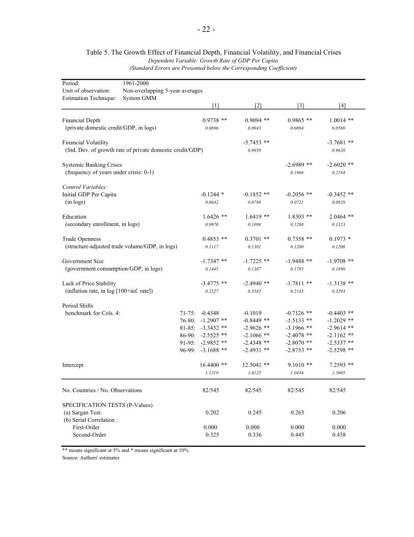
Table 5 reports the regression estimation results as well as the Sargan and serial-correlation specification tests. These tests indicate that the hypothesis of correct identification cannot be rejected, thus supporting the estimation results to which we turn next. The first column presents the results of a typical growth regression. It confirms the negative growth impact of initial GDP per capita (conditional convergence), the size and burden of government, and monetary instability through high inflation. It also shows the positive growth effect of education investment, international trade openness, and, most importantly for our purposes, financial depth. The period shifts are also significant and indicate that world conditions deteriorated in the last twenty years making it more difficult for countries to grow in the 1980s and 1990s than in the previous decades. The second and third columns include, respectively, financial volatility and the frequency of systemic banking crises as additional explanatory variables. The fourth column includes both indicators of financial fragility at the same time. Whether individually or together, financial volatility and the frequency of banking crises present a significantly negative coefficient. Financial depth maintains its positive and significant coefficient in all regressions. We can get a broad sense of the economic importance of these effects by using the point estimate of the regression coefficients to calculate the growth impact of a change in our financial measures. An increase in financial volatility by one standard deviation leads to a decrease of 0.3 percentage points in the annual growth rate of GDP per capita, and an analogous increase in the frequency of systemic banking crises produces a 0.7 percentage point drop in annual growth. On the other hand, an increase in financial depth by one standard deviation leads to economic growth by 0.9 percentage points. Naturally, these are ceteris paribus calculations, and our conjecture is that the total effect of financial liberalization and intermediation may be a combination of these effects, with weights for financial depth and financial fragility depending on the country’s stage of financial development.

- 22 -

Period: 1961-2000Unit of observation: Non-overlapping 5-year averagesEstimation Technique: System GMM

[1] [2] [3] [4]

Financial Depth 0.9738 ** 0.9094 ** 0.9865 ** 1.0014 ** (private domestic credit/GDP, in logs) 0.0896 0.0943 0.0894 0.0569

Financial Volatility -5.7453 ** -3.7681 ** (Std. Dev. of growth rate of private domestic credit/GDP) 0.9959 0.9638

Systemic Banking Crises -2.6989 ** -2.6020 ** (frequency of years under crisis: 0-1) 0.1966 0.2184

Control Variables:Initial GDP Per Capita -0.1244 * -0.1852 ** -0.2056 ** -0.3452 ** (in logs) 0.0642 0.0788 0.0721 0.0928

Education 1.6426 ** 1.6419 ** 1.8303 ** 2.0464 ** (secondary enrollment, in logs) 0.0970 0.1098 0.1288 0.1323

Trade Openness 0.4853 ** 0.3701 ** 0.7358 ** 0.1973 * (structure-adjusted trade volume/GDP, in logs) 0.1117 0.1301 0.1200 0.1206

Government Size -1.7347 ** -1.7225 ** -1.9488 ** -1.9708 ** (government consumption/GDP, in logs) 0.1445 0.1387 0.1785 0.1898

Lack of Price Stability -3.4775 ** -2.4940 ** -1.7811 ** -1.3138 ** (inflation rate, in log [100+inf. rate]) 0.2527 0.3582 0.2143 0.3293

Period Shifts benchmark for Cols. 4: 71-75: -0.4348 -0.1019 -0.7126 ** -0.4403 **

76-80: -1.2907 ** -0.8449 ** -1.5133 ** -1.2029 **81-85: -3.3432 ** -2.9626 ** -3.1966 ** -2.9614 **86-90: -2.5525 ** -2.1066 ** -2.4078 ** -2.1162 **91-95: -2.9852 ** -2.4348 ** -2.8070 ** -2.5337 **96-99: -3.1688 ** -2.4931 ** -2.8753 ** -2.5298 **

Intercept 16.4400 ** 12.5041 ** 9.1010 ** 7.2593 **1.1319 1.6125 1.0434 1.5605

No. Countries / No. Observations 82/545 82/545 82/545 82/545

SPECIFICATION TESTS (P-Values) (a) Sargan Test: 0.202 0.245 0.263 0.206 (b) Serial Correlation : First-Order 0.000 0.000 0.000 0.000 Second-Order 0.325 0.336 0.445 0.438

** means significant at 5% and * means significant at 10%Source: Authors' estimates

Table 5. The Growth Effect of Financial Depth, Financial Volatility, and Financial Crises Dependent Variable: Growth Rate of GDP Per Capita

(Standard Errors are Presented below the Corresponding Coefficient)

- 23 -

IV. CONCLUSIONS

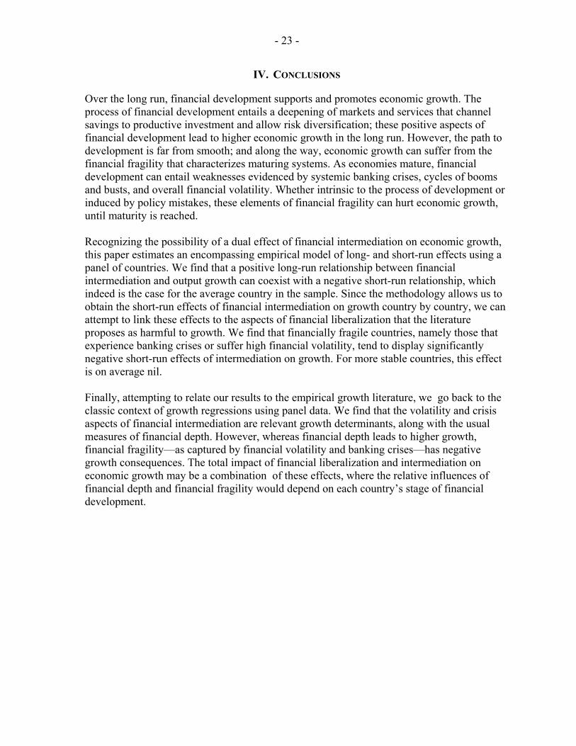
Over the long run, financial development supports and promotes economic growth. The process of financial development entails a deepening of markets and services that channel savings to productive investment and allow risk diversification; these positive aspects of financial development lead to higher economic growth in the long run. However, the path to development is far from smooth; and along the way, economic growth can suffer from the financial fragility that characterizes maturing systems. As economies mature, financial development can entail weaknesses evidenced by systemic banking crises, cycles of booms and busts, and overall financial volatility. Whether intrinsic to the process of development or induced by policy mistakes, these elements of financial fragility can hurt economic growth, until maturity is reached. Recognizing the possibility of a dual effect of financial intermediation on economic growth, this paper estimates an encompassing empirical model of long- and short-run effects using a panel of countries. We find that a positive long-run relationship between financial intermediation and output growth can coexist with a negative short-run relationship, which indeed is the case for the average country in the sample. Since the methodology allows us to obtain the short-run effects of financial intermediation on growth country by country, we can attempt to link these effects to the aspects of financial liberalization that the literature proposes as harmful to growth. We find that financially fragile countries, namely those that experience banking crises or suffer high financial volatility, tend to display significantly negative short-run effects of intermediation on growth. For more stable countries, this effect is on average nil. Finally, attempting to relate our results to the empirical growth literature, we go back to the classic context of growth regressions using panel data. We find that the volatility and crisis aspects of financial intermediation are relevant growth determinants, along with the usual measures of financial depth. However, whereas financial depth leads to higher growth, financial fragility—as captured by financial volatility and banking crises—has negative growth consequences. The total impact of financial liberalization and intermediation on economic growth may be a combination of these effects, where the relative influences of financial depth and financial fragility would depend on each country’s stage of financial development.

- 24 - APPENDIX I

Full Sample (75 countries)

Restricted Sample (66 countries)

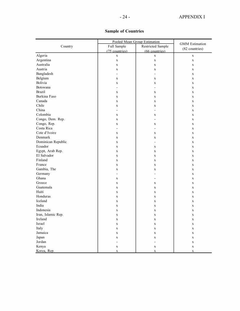
Algeria x x xArgentina x x xAustralia x x xAustria x x xBangladesh - - xBelgium x x xBolivia x x xBotswana - - xBrazil x x xBurkina Faso x x xCanada x x xChile x x xChina - - xColombia x x xCongo, Dem. Rep. x - xCongo, Rep. x x xCosta Rica - - xCote d' Ivoire x x xDenmark x x xDominican Republic x - xEcuador x x xEgypt, Arab Rep. x x xEl Salvador x x xFinland x x xFrance x x xGambia, The x x xGermany - - xGhana x - xGreece x x xGuatemala x x xHaiti x x xHonduras x x xIceland x x xIndia x x xIndonesia x x xIran, Islamic Rep. x x xIreland x x xIsrael x x xItaly x x xJamaica x x xJapan x x xJordan - - xKenya x x xKorea, Rep. x x x

Pooled Mean Group Estimation GMM Estimation (82 countries)

Country

Sample of Countries

- 25 - APPENDIX I

Full Sample (75 countries)

Restricted Sample (66 countries)

Madagascar x x xMalawi x x xMalaysia x x xMexico x x xMorocco x x xNetherlands x x xNew Zealand x x xNicaragua x x xNiger x x xNigeria x x xNorway x x xPakistan x x xPanama x x xPapua New Guinea - - xParaguay x x xPeru x x xPhilippines x x xPortugal x x xSenegal x - xSierra Leone x - xSingapore x x xSouth Africa x x xSpain x x xSri Lanka x x xSweden x x xSwitzerland x x xSyrian Arab Republic x x xThailand x - xTogo x x xTrinidad and Tobago x x xTunisia x x xTurkey x - xUganda x - -United Kingdom x x xUnited States x x xUruguay x x xVenezuela, RB x x xZambia x - xZimbabwe - - x

Pooled Mean Group Estimation GMM Estimation (82 countries)

Country

Sample of Countries

- 26 - APPENDIX II

Variable Definition and Construction SourceGDP per capita Ratio of total GDP to total

population. GDP is in 1985 PPP-adjusted US$.

Authors' construction using Summers and Heston (1991) and World Bank (2002).

GDP per capita growth Log difference of real GDP per capita.


Initial GDP per capita Initial value of ratio of total GDP to total population. GDP is in 1985 PPP-adjusted US$.


Education Ratio of total secondary enrollment, regardless of age, to the population of the age group that officially corresponds to that level of education.

World Development Network (2002) and World Bank (2002).

Private credit Ratio of domestic credit claims on private sector to GDP

Author’s calculations using data from International Financial Statistics (IFS), the publications of the central bank and Penn World Tables (PWT). The method of calculations is based on Beck, Demirguc-Kunt and Levine (1999).

Trade openness Residual of a regression of the log of the ratio of exports and imports (in 1995 US$) to GDP (in 1995 US$), on the logs of area and population, and dummies for oil exporting and for landlocked countries.

Author’s calculations with data from World Development Network (2002) and World Bank (2002).

Government size Ratio of government consumption to GDP.

World Bank (2002).

CPI Consumer price index (1995 = 100) at the end of the year

Author’s calculations with data from International Financial Statistics .

Inflation rate Annual % change in CPI Author’s calculations with data from International Financial Statistics .

Systemic banking crises Number of years in which a country underwent a systemic banking crisis, as a fraction of the number of years in the corresponding period.

Author’s calculations using data from Caprio and Klingebiel (1999), and Kaminsky and Reinhart (1998).

Period-specific shifts Time dummy variables. Authors’ construction.

Definitions and Sources of Variables Used in Regression Analysis

- 27 - APPENDIX III

(a) U

niva

riat

eD

ata

in 5

-Yea

r Pe

riods

Dat

a in

1-Y

ear

Perio

ds82

Cou

ntrie

s, 5

45 O

bser

vatio

ns75

Cou

ntrie

s, 2

908

Obs

erva

tions

Mea

nSt

d. D

ev.

Min

.M

ax.

Mea

nSt

d. D

ev.

Min

.M

ax.

Gro

wth

rat

e of

GD

P pe

r ca

pita

1.61

422.

7577

-10.

9242

10.1

276

1.80

444.

4232

-33.

8733

35.4

460

Priv

ate

dom

estic

cre

dit/G

DP

(in lo

gs)

3.37

520.

8944

-1.0

841

5.43

463.

2808

0.93

53-1

.512

85.

4680

Initi

al G

DP

per

capi

ta (i

n lo

gs)

7.77

511.

5594

4.97

6910

.735

47.

7432

1.57

534.

7932

10.7

531

Stru

ctur

e-ad

juste

d tra

de v

olum

e/G

DP

(in lo

gs)

0.04

530.

4902

-1.4

605

1.44

54-0

.006

50.

5572

-2.8

184

1.82

85G

over

nmen

t con

sum

ptio

n /G

DP

(in lo

gs)

2.64

380.

3778

1.45

643.

6370

2.60

180.

3786

1.12

753.

9985

Infla

tion

(in

log

[100

+in

f. r

ate]

)4.

7341

0.17

444.

5851

6.13

524.

7250

0.18

053.

9158

6.47

52St

d. D

ev. o

f gro

wth

of p

rivat

e cr

edit/

GD

P0.

0854

0.07

410.

0072

0.70

54Fr

eque

ncy

of y

ears

und

er b

anki

ng c

risis

0.11

300.

2685

0.00

001.

0000

Seco

ndar

y en

rollm

ent (

in lo

gs)

3.64

180.

8365

0.11

264.

9231

(b) B

ivar

iate

Cor

rela

tions

. D

ata

in 5

-Yea

r pe

riod

s, 8

2 co

untr

ies

(low

er le

ft tr

iang

ular

mat

rix)

and

Dat

a in

1-Y

ear

peri

ods

(upp

er r

igth

tria

ngul

ar m

atri

x)

Gro

wth

rat

e of

GD

P pe

r ca

pita

Priv

ate

dom

estic

cr

edit/

GD

P (in

logs

)

Initi

al G

DP

per

capi

ta (i

n lo

gs)

Stru

ctur

e-ad

just

ed

trade

vo

lum

e/G

DP

(in lo

gs)

Gov

ernm

ent

cons

umpt

ion

/GD

P (in

lo

gs)

Infla

tion

(in

log

[100

+in

f.

rate

])

Std.

Dev

. of

grow

th o

f pr

ivat

e cr

edit/

GD

P

Freq

uenc

y of

ye

ars

unde

r ba

nkin

g cr

isis

Seco

ndar

y en

rollm

ent

(in lo

gs)

Gro

wth

rat

e of

GD

P pe

r ca

pita

10.

1229

6489

80.

150.

03-0

.048

8839

8-0

.2Pr

ivat

e do

mes

tic c

redi

t/GD

P (in

logs

)0.

291

0.72

0.09

0.38

8084

107

-0.3

3548

991

Initi

al G

DP

per

capi

ta (i

n lo

gs)

0.23

0.71

1-0

.17

0.41

-0.1

1St

ruct

ure-

adju

sted

trad

e vo

lum

e/G

DP

(in lo

gs)

0.07

0.1

-0.1

81

0.2

-0.2

1G

over

nmen

t con

sum

ptio

n /G

DP

(in lo

gs)

-0.0

40.

350.

410.

231

0.2

Infla

tion

(in

log

[100

+in

f. r

ate]

)-0

.35

-0.4

-0.1

3-0

.27

-0.0

91

Std.

Dev

. of g

row

th o

f priv

ate

cred

it/G

DP

-0.3

7-0

.45

-0.3

60

-0.0

40.

481

Freq

uenc

y of

yea

rs u

nder

ban

king

cris

is-0

.26

-0.1

2-0

.15

0.03

-0.1

0.27

0.26

1Se

cond

ary

enro

llmen

t (in

logs

)0.

210.

580.

78-0

.06

0.35

-0.0

2-0

.23

0.02

1

Sour

ce: A

utho

rs' c

alcu

latio

ns

Des

crip

tive

Stat

istic

s

- 28 -

REFERENCES

Aghion, Philippe, Philippe Bacchetta, and Abhijit Banerjee (forthcoming), “Capital Markets and the Instability of Open Economies,” Journal of Monetary Economics.

Alonso-Borrego, Cesar, and Manuel Arellano, 1999, “Symmetrically Normalized Instrumental-Variable Estimation Using Panel Data,” Journal of Business & Economic Statistics, Vol.17, pp. 36–49.

Arellano, Manuel, and Stephen Bond, 1991, “Some Tests of Specification for Panel

Data: Monte Carlo Evidence and an Application to Employment Equations,” Review of Economic Studies, Vol. 58, pp. 277–97.

Arellano, Manuel, and Olympia Bover, 1995, “Another Look at the Instrumental-

Variable Estimation of Error-Components Models,” Journal of Econometrics, Vol. 68, pp. 29–51.

Attanasio, Orazio, Lucio Picci, and Antonello Scorcu, 2000, “Saving, Growth and

Investment: A Macroeconomic Analysis Using a Panel of Countries,” Review of Economics and Statistics, Vol. 82 (2), pp.182–211.

Balino, Tomas, and V. Sundararajan, 1991, editors, Banking Crises: Cases and Issues,

Washington: International Monetary Fund. Barro, Robert, 2000, “Economic Growth in a Cross Section of Countries,” Quarterly

Journal of Economics, Vol.106 (2) pp. 407–43. Beck, Thorsten, Asli Demirguc-Kunt, and Ross Levine, 2000, “A New Database on

Financial Development and Structure,” World Bank Economic Review, 14 (3), pp. 597–605.

Beck, Thorsten, Ross Levine, and Norman Loayza, 2000, “Financial Development and

the Sources of Growth,” Journal of Financial Economics, Vol. 58 (1-2), pp. 261–300.

Bencivenga, Valerie, and Bruce Smith, 1991, ''Financial Intermediation and Endogenous

Growth,” Review of Economic Studies, 58, pp.195–209.

Blundell, Richard, and Stephen Bond, 1998, “Initial Conditions and Moment Conditions in Dynamic Panel Data Models,” Journal of Econometrics, Vol. 87, pp.115–43.

Caprio, Gerard, and Daniela Klingebiel, 1996, “Bank Insolvencies: Cross-Country

Experience,” World Bank Policy Research Working Paper No. 1620. ———, 2003, “Episodes of Systemic and Borderline Financial Crises” (unpublished;

Washington: The World Bank).

- 29 -

Caselli, Francesco, Gerardo, Esquivel, and Fernando Lefort, 1996, “Reopening the Convergence Debate: A New Look at the Cross-Country Growth Empirics,” Journal of Economic Growth, 1 (3), pp. 363–89.

Demirguc-Kunt, Asli, and Enrica Degatriache, 1998, “The Determinants of Banking

Crises in Developing and Developed Countries,” International Monetary Fund Staff Papers, Vol. 45 (1) pp. 81–109.

———, 2000, “Banking Sector Fragility: A Multivariate Logit Approach” World Bank

Economic Review, 14 (2), pp. 287–307.

De Gregorio, Jose, and Pablo Guidotti, 1995, “Financial Development and Economic Growth,” World Development, 23(3), p. 433–48.

Dell’Ariccia, Giovanni and Robert Marquez, 2004a, “Lending Booms and Lending

Standards,” (unpublished). ———, 2004b, “Information and Bank Credit Allocation,” Journal of Financial

Economics, 72 (1), pp.185–214. Eichengreen, Barry, and Andrew Rose, 1998, “Staying Afloat When the Wind Shifts:

External Factors and Emerging-Market Banking Crises,” NBER Working Paper 6370 (Cambridge, Massachusetts: National Bureau of Economic Research).

Gavin, Michael, and Ricardo Hausmann, 1998, “The Roots of Banking Crises: The

Macroeconomic Context,” in Banking Crises in Latin America, Ricardo Hausmann and Liliana Rojas-Suarez, editors, Washington: Interamerican Development Bank.

Gaytan, Alejandro, and Romain Rancière, 2003, “Banks, Liquidity Crises and Economic

Growth,” (unpublished). Gourinchas, Pierre-Olivier, Oscar Landerretche, and Rodrigo Valdes, 2001, “Lending

Booms: Latin America and the World,” Economia, 1 (2), pp. 47–100.

Greenwood, Jeremy, and Boyan Jovanovic, 1990, “Financial Development, Growth, and the Distribution of Income,” Journal of Political Economy, Vol. 98, pp.1076–107.

Griliches, Zvi, and Jerry Hausmann, 1986, "Errors in Variables in Panel Data," Journal of

Econometrics, Vol. 31, pp. 93–118. Hnatkovska, Viktoria, and Norman Loayza, (forthcoming), “Volatility and Growth,” in

Managing Volatility and Crises: A Practitioner’s Guide, edited by Joshua Aizenman and Brian Pinto; Cambridge University Press.

Holtz-Eakin, Douglas, Newey Whitney, and Harvey Rosen, 1988, “Estimating Vector

Autoregressions with Panel Data,” Econometrica, 56 (6), pp. 1371–95.

- 30 -

Johansen, Soren, 1995, “Likelihood Based Inference of Cointegration in the Vector Error Correction Mode,” Oxford University Press.

Kaminsky, Graciela, and Carmen Reinhart, 1999, “The Twin Crises: The Causes of

Banking and Balance of Payments Problems,” American Economic Review, Vol. 89, No. 3, pp. 473–500.

King, Robert, and Ross Levine, 1993a, “Finance and Growth: Schumpeter Might Be

Right,” Quarterly Journal of Economics, Vol.153(3), pp. 717–38.

———, 1993b, "Finance, Entrepreneurship, and Growth: Theory and Evidence," Journal of Monetary Economics, Vol. 32 (3), pp. 513–42.

Levine, Ross, Norman Loayza, and Thorsten Beck, 2000, “Financial Intermediation and

Growth: Causality and Causes,” Journal of Monetary Economics, 46 (1), pp. 31–77.

Pesaran, Hashem, 1997, “The Role of Econometric Theory in Modeling the Long Run,” Economic Journal, 107, pp.178–191.

———, and Ron Smith, 1995, “Estimating Long-Run Relationships from Dynamic

Heterogeneous Panels,” Journal of Econometrics, 68 (1995), pp. 79–113. ———, ———, and Kyung Im, 1996, “Dynamic Linear Models for Heterogenous

Panels,” The Econometrics of Panel Data, L. Matyas and P. Sevestre, editors, pp.145–195, (Dordrecht: Kluwer Academic Publishers).

———, and Yongcheol Shin, 1999, “An Autoregressive Distributed Lag Modelling

Approach to Cointegration,” Chapter 11 in Econometrics and Economic Theory in the 20th Century; The Ragnar Frisch Centennial Symposium, Cambridge University Press.

Pesaran, Hashem, Yongcheol Shin, and Richard Smith, 1999, “Pooled Mean Group

Estimation of Dynamic Heterogeneous Panels,” Journal of the American Statistical Association, 94, pp. 621–34.

Philipps, Peter, and Bruce Hansen, 1990, “Statistical Inference in Instrumental Variables

Regression with I(1) Processes,” The Review of Economic Studies, 57 (1), pp. 99–125. Rajan, Raghuram, 1994, "Why Bank Credit Policies Fluctuate: A Theory and Some

Evidence," Quarterly Journal of Economics, 109, pp. 399–442

Robertson, Donald, and James Symons, 1992, “Some Strange Properties of Panel Data Estimators,” Journal of Applied Econometrics, 7, pp.175–89.

Roubini, Nouriel, and Xavier Sala-i-Martin, 1992, “Financial Repression and Economic

Growth,” Journal of Development Economics, Vol. 39 (1), pp. 5–30.

- 31 -

Sachs, Jeffrey, Aaron Tornell, and Andres Velasco, 1996, “Financial Crises in Emerging

Markets: The Lessons from 1995,” Brookings Papers on Economic Activity, pp. 147–98. Schneider, Martin, and Aaron Tornell, (2004), “Balance Sheet Effects, Bailout

Guarantees and Financial Crises,” Review of Economic Studies Vol. 71, pp. 883–913.

Wynne, Jose, 2002, “Information Capital, Firm Dynamics and Macroeconomic

Performance,” (unpublished).

financial development, financial fragility, and growth · wp/05/170 financial development,...

Documents