final report of the opgt/mjs plasma wave science team · · 2013-08-31final report of the...
TRANSCRIPT

1 September 1972
FINAL REPORT OF THE OPGT/MJSPLASMA WAVE SCIENCE TEAM
Prepared by
F. L. Scarf, Team Leader
for
National Aeronautical and Space AdministrationWashington, D.C. 205*t6
Contract NASW 2228
Space Sciences Department
TRW Systems GroupOne Space Park
Redondo Beach, California 902?84
https://ntrs.nasa.gov/search.jsp?R=19720026115 2018-06-27T17:55:37+00:00Z

Page 1
1. TEAM ORGANIZATION AND MEMBERSHIP
The Plasma Wave Team Leader is Dr. F. L. Scarf of TRW Systems, and the
official team members are Dr. D. A. Gurnett (University of Iowa), Dr. R. A.
Helliwell (Stanford University), Dr. R. E. Holzer (UCLA), Dr. P. J. Kellogg
(University of Minnesota), Dr. E. J. Smith (JPL), and Dr. E. Ungstrup (Danish
Space Research Institute). Mr. A. M. A. Frandsen of JPL serves as Team Member
and Experiment Representative.
In addition, the Plasma Wave Team solicited the continuing support and
assistance of several other outstanding scientists, and we have designated
these participants as Team Associates; the Associates are Dr. N. M. Brice
(Cornell University), Dr. D. Cartwright (University of Minnesota), Dr. R. W.
Fredricks (TRW), Dr. H. B. Liemohn (Boeing), Dr. C. F. Kennel (UCLA), and
Dr. R. Thome (UCLA) .
2. GENERAL TEAM ACTIVITIES FEBRUARY 1972-AUGUST 31, 1972(See the mid-year report for a summary of the earlier work)
During this period Dr. Scarf attended all SSG Meetings except the last
one, where Dr. E. J. Smith represented the Plasma Wave Team. There were a
number of Team Meetings and several additional .conferences at JPL concerning
EMI and other potential spacecraft problems.
The major development during this interval involved the decision not to
go ahead with the Grand Tour. The change to the Mariner Jupiter/Saturn Mis-
sion required some redirection of the Headquarters-funded supporting studies.
In particular, for the MJS 77 Jupiter flybys at L = 5.8 and L = 7-2, the

Page 2
radiation hazard was no longer considered to be severe, and we terminated the
JPL studies of radiation tolerance. Instead, the JPL Team Members focused
attention on EMI problems and on the problems that developed in trying to fit
a shielded magnetic search coil on the Mariner Astromast.
Dr. Scarf also redirected his efforts to study characteristics of the
Saturn and Jupiter flybys, instead of considering all outer planets.
The general Stanford University study proceeded without .change.
3. RESULTS
Our results are described in detail in a series of Appendices. Here we
briefly summarize the contents of the individual sections.
1. A detailed study of the Plasma Environment and Magnetosphere of
Saturn was carried out. The report is contained in Appendix 1. This paper
was submitted to Cosmic Electrodynamics and is now in press.
2. Dr. Scarf analyzed the possible electrical hazards associated with
differential spacecraft charging during the MJS flyby of Jupiter. A memo was
transmitted to the Project, and a copy is contained in Appendix 2.
3. Dr. Scarf, Dr. Smith, and Mr. Frandsen conferred with the MJS Pro-
ject on potential EMI problems and helped prepare specifications for the AFO
package. Some memos on this topic are contained in Appendix 3.
k. Dr. Scarf prepared a handout for the final SSG Meeting, and Dr.
Smith circulated this Summary of the Plasma Team effort to Headquarters per-»
sonnel. A copy is contained in Appendix k.

Page 3
5. The Stanford Study directed by Dr. Helliwell was completed, and a
Final Report is attached as Appendix 5.

18864-6004-RO-OO
APPENDIX 1
to
FINAL REPORT OF THE OPGT/MJS
PLASMA WAVE SCIENCE TEAM

18864-6003-RO-OO
SOME COMMENTS ON THE MAGNETOSPHERE AND PLASMA
ENVIRONMENT OF SATURN
by
Frederick L. ScarfSpace Sciences Department
20 April 1972
'Space Sciences DepartmentTRW Systems GroupOne Space Park
Redondo Beach, California 90278

Page i
SOME COMMENTS ON THE MAGNETOSPHERE AND PLASMA
ENVIRONMENT OF SATURN
ABSTRACT
Some properties of a model magnetosphere for Saturn are studied in order
to determine the bounds that can be set on the surface field strength and the
trapped particle population. The primary observational constraint is that
non-thermal radiation similar to the Jovian radio emissions must be undetect-
able from Earth. It is argued that for a Saturn surface field of approxi-
mately one gauss, those particles that are energized as they diffuse in from
the magnetopause with conservation of magnetic moment will produce synchro-
tron radiation levels that are undetectable at a range of 9.5 AU. The plasma
instabilities that heat the oncoming wind particles at the bow shock and
others that can limit the stably-trapped flux levels are also discussed
briefly.

SOME COMMENTS ON THE MAGNETOSPHERE AND PLASMA
ENVIRONMENT OF SATURN
1. INTRODUCTION
There is no direct evidence that the solar wind flows out to 9.5 AU in
an ordered manner^ but almost all theories of the heliosphere termination
indicate that Saturn should be immersed in the wind (Axford, 1972). We also
have no direct evidence that the magnetic moment of Saturn is finite, but
the great physical similarities between Saturn and Jupiter suggest that it
is very dangerous to assume that Saturn is unmagnetized. Therefore, we make
the plausible assumptions that Saturn is magnetized and exposed to the solar
wind, and we can then proceed toward construction of a general model for the
planetary magnetosphere and trapped radiation belts. The single observational
•constraint, that Saturn should not produce non-thermal radio emission detect-
able on earth (Gulkis et a!., 1969) appears easy to satisfy if we use the
same type of reasoning that apparently works for Jupiter.
This note contains an outline of these-concepts. In Section 2, the
properties of the solar wind at 9.5 AU are considered. Section 3 contains
an initial evaluation of the magnetospheric configuration, trapped radiation
belts, and synchrotron emission for a one-gauss Saturn surface field. The
role of plasma waves in controlling the wind-magnetosphere interaction and
the trapped particle population of Saturn is discussed in Section 4. In the
final section we summarize our considerations, and we argue that Saturn can
indeed possess a significant magnetosphere with a sizeable trapped particle
population. Thus, the non-detection of radio emission from Saturn must not
be interpreted as evidence that Saturn has no magnetosphere.

Page 2
2. " THE SOLAR WIND AT 9.5 AU
No matter what general type of interaction occurs between a planetary
object and the solar wind, the shock or interface actually forms within the
interplanetary plasma. If the object is big enough, as Saturn certainly is,
then a bow shock will develop, even for B = 0; in order to assess what this
shock will look like, we have to know the ambient interplanetary characteris-
ti cs.
It is actually a straightforward matter to extrapolate some solar wind
parameters over the 1 AU to 9.5 AU range. We assume V(wind) = const (no
heliosphere termination or neutral hydrogen "friction"), and this gives N(r) ^- 2 - 1 2r . The same reasoning tells us that B ^ r , BQ r (the Parker model),
and we readily find the numbers that are contained in Table 1, but some
further comments are required to explain the significance of the last two
entries.
Near Earth, the interplanetary right-hand polarized (n2 = R) electron
whistler mode wave appears to play a significant role in providing a dc mag-
netic field jump at the bow shock. For f - f_"/2, this wave has a phase speed =\f
cf /2 f " =: 900 km/sec, and this is greater than the nominal 400 km/sec windc pspeed. As f increases past f ~/2 and toward f ~ the phase speed drops and for
C C
some intermediate f (f ~/2 < f < f ~)» (w/k) = V(wind). In this case, theu c u o
Doppler-shifted frequency u>' = w. - k-V = 0, and a dc magnetic pulse stands0 tflf *»
in the wind to form a thin shock with \ - c/2?rf ~ - 2 kilometers. Table 1
shows that a similar situation can develop at Saturn, since (w/k),.,.,, at 9.5 AU =
770 km/sec is still greater than the wind speed. The main difference is that
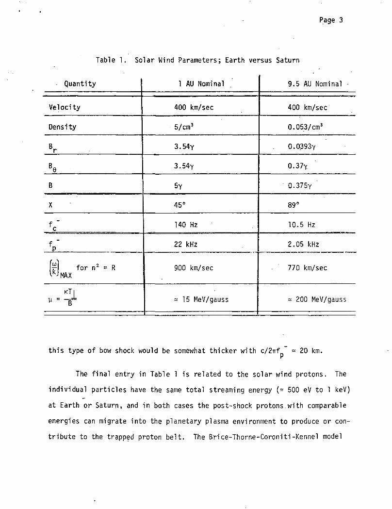
Page 3
Table 1. Solar Wind Parameters; Earth versus Saturn
Quantity
Velocity
Density
Br
V
B
X
fc"
V
(F! for "2 = RWMAXKTi
y B
1 AU Nominal
400 km/sec
5/cm3
3.54y
3.54Y
5Y
45°
140 Hz
22 kHz
900 km/sec
= 15 MeV/gauss
9.5 AU Nominal -
400 km/sec
0.053/cm3
0.0393Y
0.37Y
0.375Y
89°
10.5 Hz
2.05 kHz
770 km/sec
= 200 MeV/gauss
this type of bow shock would be somewhat thicker with c/2irf ~ = 20 km.
The final entry in Table 1 is related to the solar wind protons. The
individual particles have the same total streaming energy (= 500 eV to 1 keV)
at Earth or Saturn, and in both cases the post-shock protons.with comparable
energies can migrate into the planetary plasma environment to produce or con-
tribute to the trapped proton belt. The Brice-Thorne-Coroniti-Kennel model

Page 4
of the Jupiter proton belts (Brice, 1972; Thorne and Corom'tl, 1972; Kennel.
1972) is based on diffusion with conservation of y = mvi2/B. Here we note
that u at Saturn is huge in comparison with the 1 AU value.
The thermal state of the solar wind at Saturn is much more uncertain.
At 1 AU, we already have T_ t \ (T,,)_ + (T,)_, (Tii/T,)_ i (Tii/T,)+, where
prefer to electrons and protons, and the parallel-perpendicular subscripts
refer to directions for thermal fluctuation speeds with respect to the mag-
netic field orientation. We don't really know how to account for the 1 AU
temperatures, and any extrapolation is highly speculative. However, a number
of simple physical models can be used. For instance, we can neglect the
anisotropies (i.e., assume K+ = (Tii/T|)+ - 1) and neglect the electron-— II j_ ~proton temperature difference. Then a one-fluid (singly) adiabatic model
gives P = NKT ^ NY, or T ^ r^. For y = 3/2, T(r) ^ r . A two-fluid
generalization of this is obvious, and a more sophisticated two-fluid "double
adiabatic" model has KT_/B = constant, icT,, B2/N2 = constant, for electrons and
protons separately (see, for instance, Scarf, 1969). The results of these nu-
merical explorations are gathered in Table 2, and several points are worth noting,
1 /2a) In all cases, A_ = (2i<T_/m) ' is quite low near Saturn, in compari-
son to the solar wind flow speed. For fast streams we could see V(wind) =
A . This is very significant because high frequency electrostatic plasma
waves with f = f have phase speeds near A . Thus, w^ = u - k*V can be nearp - «»• *>
zero in the planet frame, and a dc electric field jump can provide a new type
of bow shock.

Table 2
Page 5
Quantity
<T>
\
A_
<V
A+
<T_>
A_
•<V|
(T+)J_
K+
\
<T.)||
<T.>1
K_
A_
1 AU
105°K
41 km/sec
1750 km/sec
5 x lO^K
29 km/sec
1.5 x 10⁵°K
2140 km/sec
7.5 x 10*°K
3 x 10"°K
2.5
29 km/sec
1.6 x 1050K
1.4 x 10⁵°K
1.14
2140 km/sec
9.5 AU
1.05 x lO^K
13.3 km/sec
570 km/sec
5.2 x 10³°K
9.5 km/sec
1.6 x lO^K
690 km/sec
1.5 x 10³oK
2.24 x 10³°K
0.67
5.8 km/sec
3.45 x 10"°k
1.05 x lO^K
0.314
550 km/sec
One-fluidsingly adiabatic
Y = 3/2
Two-fluidsingly adiabatic
Y = 3/2
Two-fluiddoubly adiabatic
Page 6
b) Near Earth K+ > 1, K £1, and the solar wind is a plasma that is
unstable with respect to growth of magnetosonic waves (the Firehose) and low
frequency (f - f ) electron whistler mode waves (Kennel and Scarf, 1968).C '
With the double adiabatic model, K+ < 1 and K_ < 1 at r = 9.5 All. In this
case the solar wind is again unstable, but completely different plasma waves
grow spontaneously. For K± < 1, we should expect growth of ion and electron
cyclotron waves (n2 = L, f - f , and n2 = R, f - f ~)> and the wind at 10 AU
should therefore be fundamentally different from that near earth (-see also,
Scarf. 1969).
3. THE MAGNETOSPHERE OF SATURN !
Let us assume that Saturn has a centered dipole with moment M = 2.16 x
1029 cgs units and equatorial surface magnetic field equal to one gauss. This
assumption is convenient and plausible because:
a) The f " value at the surface is 2.8 MHz. If Saturn does have deca-
roetric-type radio emission, it would be invisible from Earth in this frequency
range.
b) This value for B (r ) is about equal to one obtained with the as-5 *>
sumption that the magnetic moment is proportional to the angular momentum.
While a magnetic "Bode's Law" may be open to severe questioning for general
applicability, it seems reasonable when we are merely comparing Saturn to
Jupiter. •-
c) Brice and Ioannidis.(1970, 1971) have carried out many calculations
of magnetospheric shape, corotation effects, etc. for a one-gauss surface
field plus a 10-hour spin period, and it is convenient to be able to draw on
these reports.

Page 7
With this assumption we can locate the subsolar magnetopause R-value
using (Nra+v2)wl-ncj
= RS6B 2(R=Rs)/8TrR
6. Using the parameters of Table 1 we
then find R(mpause) = 39 R = 2.4 million kilometers. Thus, Saturn's mag-
netosphere can be intermediate between that of Earth (R = 10 R ) and that of
Jupiter (R * 53 R,). The crucial question concerns the trapped population of
Saturn's belts. What fluxes will be present? What will the particle energy
distributions be? Why are non-thermal radio emissions undetectable?
Let us first consider the protons and their energies. As in the case
of Jupiter (Brice, 1972, and the other Workshop papers), we assume that some
fraction of the solar wind or magnetosheath population diffuses across a
porous magnetopause conserving u. If the particles then diffuse down to L =
2 (the known outer limit of the A-ring), still conserving y, then E/. 2\ -
^sheath) [B(L=2)/B(sheath)]' At Saturn> B(sheath) 1s rou9h1^ one-half of
the value at Jupiter (i.e., B(interDlanetarv) at 9'5 AU is about half the
value at 5.2 All), but we have assumed B(surface} at Saturn is one-twelfth of
the value at Jupiter. This means E+ (Saturn, L=2) = E+ (Jupiter, L=2)/6.
The upper limit Jupiter models of Brice (1972), Thome and Coroniti (1972),
and Kennel (1972) give a characteristic proton energy of 100 MeV at L = 2,
and therefore at Saturn E (L=2) == E (maximum) might be near 15 MeV.
We can use precisely this idea to scale the electrons for Saturn. The
cited upper limit model, and interpretations of Jovian radio emissions, give
E~(L=2, Jupiter) - 20 MeV, so that at Saturn we would not expect E~(L=2) =
E~(max) to be much greater than 3 MeV.

Page 8
In fact, the origin of the high electron energy is rather obscure at
Jupiter, and this number might well be an overestimate for Saturn, even if
B (L=l) = 1 gauss. The point is that the solar wind electrons originally
have very low values of y = mVi2/B. At Jupiter the incident electrons have
T_ - 8 x 10³°K, or y = <T~/B - 0.1 MeV/gauss. A theory of the electron belts
of Jupiter similar to the diffusion theory of the proton belts seems to require
that the electrons become greatly energized at the shock so that y~ jumps to
perhaps 10 MeV/gauss in the Jovian magnetosheath.
However, at Saturn the electrons in the wind still have only about
0.1 MeV/gauss (T and B go as r~ ), and as we have seen in Section 2, the bow
shock at Saturn may be vastly different from the one at Jupiter. It would
seem prudent to take at least E~ fixed as proportional to Bsurface x y~(wind),
and this gives E~(L=2; Saturn) * E~(L=2; Jupiter)/12 = 1.7 MeV.
This type of analysis can certainly be quite wrong in detail, but it
does suggest a very plausible explanation for the non-detection of synchrotron
radiation from Saturn. The energy radiated is
fdWdt
- 4 x 10"9 B2 sin2a E (l + -U (1)
synch 2E.
where EQ - 0.5 MeV. If E(L) ^ B(L) by diffusion with conservation of y, then
(dW/dt) ~ B " (E » E ), or'B 3 (E * 2EJ. A reduction in B from 12 gaussmax o max o(Jupiter, L=l) to one-eighth of a gauss (Saturn at L = 2, or the outer edge of
A-ring) therefore gives an intensity reduction that can exceed 108. Moreover,
if the electron energies are as low as (1-3) MeV, then the beaming effect will

Page 9
be greatly reduced. Finally, Saturn is observed at twice the distance of
Jupiter, and this also lowers the flux received at Earth. It does seem from
these considerations that we have no real reason to assume that Saturn is un-
magnetized. It is more likely that the planet resembles Jupiter, with a
weaker magnetic field that simply contains trapped particles of lower energy.
4. THE ROLE OF PLASMA WAVES ' .
Wave-particle interactions must play a crucial role in governing the
dynamics of the Saturn plasma environment, just as they do near Earth and at
Jupiter. We can list a few distinct effects as follows:
a) Wave-particle interactions directly determine the energy transfer
processes at the bow shock of Saturn. The wind is extremely dilute and cool
here, and plasma instabilities provide the only mechanism for conversion of
directed proton energy into thermal energy for magnetosheath electrons and
protons. Since the magnetosheath particles are the ones that are incident
on the magnetosphere and since they are also the basis for the ultimate ener-
getic particle population, it is clear that the bow shock wave-particle
interactions do play a fundamental role in the dynamics of the magnetosphere.
b) The incoming sheath particles become energized and anisotropic
[icT|~(L) = u~B(L)] as they diffuse across L-shells, and this diffusion requires
fluctuating E or B fields. High frequency waves allow fast (Bohm) diffusion
(i.e., orre gyradius per gyroperiod), but ULF fluctuations allow this to pro-
ceed much more slowly. The actual state is a balance of local effects; the

Page 10
distribution depends on the wave spectrum via the cross-L diffusion coeffi-
cient, and it is also dependent on the pitch-angle diffusion coefficient
(below). Thus, the total flux of trapped particles also directly depends
on the local wave characteristics.
c) The loss-cone anisotropy (Ti > Tn) must trigger ion and electron
cyclotron turbulence that causes pitch angle diffusion and particle precipi-
tation. This mechanism, which operates in the magnetosphere of the Earth
[see Kennel and Petschek (1966) and Cornwall et al. (1970)], limits the flux
of particles that can be stably trapped, and this also determines the overall
intensity of the radio emission. The particles that are in resonance with
cyclotron waves have A+ = (Ti/Tn )+ >. A = [ft ~/w - 1] , and_ J_ 1 - c c
nZ ~1
A quantitative evaluation of the stably-trapped limit for Saturn requires
knowledge of N(L). As with Jupiter, we expect a Brice-type cold plasma dis-
tribution governed by photoemission from the ionosphere and dominated by co-
rotation out to the boundary at R - 39 R$. However, a rigorous calculation of
N(L) for Saturn (with 25 percent of the Jovian photoflux and a different ion-
ospheric scale height) is not yet available: Therefore as a first working es-
timate we simply take N (L) - 0.25 N,(L), where N, is the Brice-Ioannidiss j <j
density profile. This initial model (which assumes that the reduced photoflux
yields a"corresponding reduction in photoelectron density) allows us to calcu-
late all characteristic wave frequencies in the hypothetical magnetosphere of
Saturn, and we can then also discuss the stable trapping phenomenon for Saturn.
At the end of this section we discuss some more realistic density characteris-
tics for Saturn.

Page 11
It is useful to contrast the situations at Jupiter and Saturn, and ac-
cordingly Figure 1 compares the wave frequency versus L-value plots for both
planets. Here we use B,(L=1) = 10 gauss = 10 B (L=l), N,(L) = the Brice-u S J
loannidis profile, and N (L) = Nj(L)/4. The two plots'are similar with shifts
toward lower frequencies at Saturn, and some additional specific features are
worth mentioning. In particular, it can be seen that while the surface elec-
tron gyrofrequency at Jupiter is several tens of Megahertz (well above the
Earth's ionospheric window), the model being used here predicts a surface
gyrofrequency at Saturn of 2.8 MHz, or well below the window. Thus, as
already noted at the beginning of Section 3, decametric-type radio emission
from Saturn would not be detected by Earth-based radio telescopes with this
model. However, the highest frequency emission from Saturn is probably much
less than f ~(L=1) because of the rings. If it is assumed that particles
cannot be trapped on L-shells that intersect the rings, then shells with L <$
2.3 (the outer limit of the A-ring) are removed from consideration, and the
maximum equatorial gyrofrequency for an L-shell having a stable population is
f (max) = 530 kHz. If this argument is expanded to exclude emission from, \+
I -6 4 (the possible outer limit of the During) then the highest equatorial
gyrofrequency on an L-shell containing particles is f ~(L=4) * 44 kHz, but
the critical frequency at the density peak (near L - 9-10) is f " - 45 kHz,
and so none of this wave energy would be radiated from the planet.
In the diffusion models discussed above, the magnetosheath particles
migrate inward from the dayside boundary with approximate conservation of
magnetic moment, y = mV|2/2B. Thus, A = (T|/T| ) increases with decreasing L
and wherever Equation (2) is satisfied, the cyclotron resonance instabilities

Page 12
then produce spontaneous growth of ion and electron whistler mode waves that
scatter the particles and limit the trapped flux. This instability is impor-
tant where the flux is high enough and where (B2/8irN), the minimum resonant
energy, is.less than the characteristic energy, E.(L) = y(mV|2/2) = yB(L)./ \ " "
Using the y^~'-values discussed above, the region of instability can be found
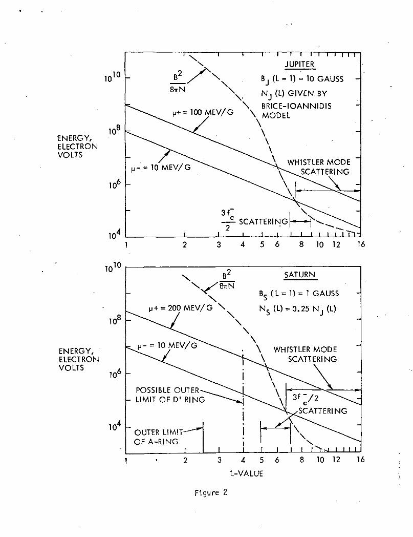
graphically, and Figure 2 shows how EI and (.B2/8-rrN) vary with L for Jupiter
and Saturn. The Jupiter plot is essentially the same as the one presented by
Thome and Coroniti (1972), but the Saturn graph utilizes a y -value twice as
large as the Jupiter one (to account for the 50 percent decrease in the inter-
planetary field at 9.5 AD), while the y~-value is kept fixed at 10 MeV/gauss
(as discussed above), it can be seen that with these specific magnetospheric
models the resonant particle instabilities can readily limit the trapped elec-
tron fluxes beyond L(Jupiter) - 7.2 or L(Saturn) =6.5.
However, the resonant-particle electromagnetic cyclotron instabilities
are not the only ones that are important in the Earth's magnetosphere.
Recently, it was found that intense electrostatic waves with f =< 3f ~/2
develop and that these emissions can provide strong diffusion and precipita-
tion for electrons (Kennel et al.. 1970; Young, 1971; Scarf et al., 1972;
Holzer and Sato, 1972). This electrostatic instability appears to develop
when (fc~/f ~) is of order unity (Oya, 1972), and Figure 1 shows that for
the models under consideration this condition occurs on slightly different
L-shells at Jupiter and Saturn. Specifically, for Jupiter (f~/f ~) equalsc p
unity near L = 7.7 while for Saturn the equality occurs near L = 5.9. Of
course, this result depends in detail on the precise B and N models adopted*
for the two planets, and the numerical prediction cannot be taken very
seriously. However, the disparity in the locations of the (f ~/f ") = 1c p

Page.13
regions does suggest an additional possible distinction between the Jupiter
and Saturn magnetospheres. As noted in Figure 2, if the 3f "/2-scattering
region for Jupiter is centered around L = 7.7.(say from L = 6.7 to L = 8.7),
then the 3f ~/2 instability overlaps the electromagnetic loss-cone instability
that already can provide strong diffusion. Thus, the second electrostatic
instability has a relatively minor effect here. However, if the electrostatic
instability at Saturn is operative from L = 4.9 to L = 6.9, for.instance, then
this additional wave-particle scattering process extends the unstable region
by a significant amount. Thus, for the Saturn model used here, it is con-
ceivable that completely stable trapping would only develop in the narrow
region between the outer limit of the A- or During, and L - 5.
Since all of these results do depend in detail on the selected N (L')
profile, it is worth considering qualitatively how a more realistic density
estimate would change the characteristic frequencies and the hypothetical
magnetosphere stability. A correct generalization of the Jupiter model has
corotating photoelectrons of ionospheric origin populating the magnetos pliers
beyond the boundary where gravitational attraction balances the centrifugal
force. At Jupiter this boundary is at about 2.2 Rj in the equatorial plane
(Brice and loannidis, 1970), but Saturn has a somewhat smaller mass, and so
for Saturn the same boundary is near r = 1.8 R . In both of the outer planet•>
cases the plasma should be in diffusive equilibrium at these radii, and any
photoelectrons that have enough energy should populate the corotation region
beyond the boundaries. However, one important correction becomes apparent
here: Since an electron in synchronous orbit around Saturn has only about
35 percent of the kinetic energy of a synchronous electron around Jupiter, a
larger fraction of the ionospheric photoelectron distribution will escape the
Page 14
gravitational barrier, and thus beyond 1.8 R the plasma density at Saturn
should be considerably higher than the value indicated by scaling the photo-
flux (I am indebted to Dr. C. F. Kennel for suggesting this important point).
Thus, use of N (L) = 0.25 N,(L) actually gives a lower density limit for thes oinner magnetosphere of Saturn? for low L-values (B2/8irN)s is expected to be
lower than the quantity shown in Figure 2, so that the inner magnetosphere of
Saturn is probably more unstable than suggested above.
Another correction is required at higher L-values because the NS(L) pro-
file should be limited by finite 3 effects. However, in Figures 1,2, the
density is reduced by a factor of four and B2 is reduced by a factor of one-
hundred, so that at high L-values, the Saturn 3 adopted here is much higher
than the reasonable values used by Brice and loannidis (1970). Thus, at
Saturn, a realistic density profile should probably peak at a somewhat lower
L-value, and it should remain lower than the 0.25 N,(L) curve beyond say L =
7. However, this change does not seriously affect the stability with respect
to whistler mode turbulence since there is already a large instability margin
beyond the peak density region.
5. DISCUSSION
Ground-based observers have never clearly detected non-thermal radio emis-
sions from Saturn at any frequencies above the Earth's 10 MHz ionospheric win-
dow (Newburn and Gulkis, 1971). This result is frequently taken to imply that
Saturn has no trapped particle belts, and in some discussions the negative
result is interpreted as evidence that Saturn has no magnetic field at all.
In fact, these conclusions do not follow from the radiometric data, and the
main purpose of the present discussion is to demonstrate that plausible models
of the Saturn magnetosphere, based on analogy with recent Jupiter models, pro-
vide no detectable radio emissions at Earth.

Page 15
The basic point is that the electrons trapped in the magnetosphere of
Jupiter attain extremely high energies (many tens of MeV) and produce such
intense synchrotron radiation only because the Jovian magnetic field strength
is so high-. If we consider an analog of Jupiter with a surface field of one
(rather than 10 or 12) gauss, then a number of phenomena combine to produce
a tremendous decrease in the radiated power levels and beaming effects. The
characteristic electron energy at a given L-shell will be down by an order
of magnitude, and the radiated power will be decreased by three or four orders
of magnitude [see Equation (1)], even if all other factors are constant. For
Saturn, there are additional potential loss mechanisms associated with the
rings, and local electromagnetic and electrostatic plasma instabilities may
independently act to limit the trapped flux levels. Finally, if the surface
field is as low as one gauss, the analog of the Jovian decametric radiation
would occur at low enough frequencies so that the Earth's ionosphere would
screen out the signal.
We conclude that the radiometric observations from Saturn are entirely
consistent with a Jupiter-type magnetosphere model having a surface field on
the order of one gauss. This result should not be surprising since the Earth,
with a substantial population of energetic particles trapped in a 0.3 gauss
surface field, provides no detectable synchrotron radiation at all. This
experimental point is quite significant, and.it is certainly well known that
synchrotron radiation from the Earth would not be intense enough to be de-
tected by an observer on Saturn. However, the case is even stronger than
this: Natural synchrotron radiation from the Earth's trapped particle belts*
has not even been clearly detected by radio experiments traversing the belts

Page .16
in Earth orbit (R. G. Stone, private communication). In fact, the onl^ unam-
biguous published accounts of synchrotron radiation from the Earth's belts
are associated with the artificial injection of relativistic electrons into
trapped orbits following the July 9, 1962 high-altitude nuclear explosion
(Ochs et al., 1963; Dyce and Horowitz, 1963; Peterson and Hower, 1963).
Thus, it is prudent to approach the problem of exploring Saturn assuming
that it does have a magnetic field and trapped particle population, with the
radiometric observations being used to set a plausible limit of about one
gauss for a surface field. There is presently no well-founded theory of
planetary magnetism that can be used to provide a better estimate, but Saturn
is somewhat smaller than Jupiter and the surface field reduction by an order
of magnitude seems reasonable. For instance, Saturn's mass, angular momentum,
and volume are about 30 percent, 22 percent, and 60 percent of the corres-
ponding quantities for Jupiter (in the respective order), so that many semi-
empirical models would predict a smaller planetary field. The use of a model
one-gauss surface field is therefore suggested until direct flyby measurements
provide more precise information.
ACKNOWLEDGMENTS
Several ideas discussed in this note were directly stimulated by the pre-
sentations of Drs. N. M. Brice, F. V. Coroniti, C. F. Kennel, and R. M. Thorne
at the Jupiter Radiation Belt Workshop. I am also grateful to Dr. Kennel for
some helpful comments about possible density distributions in the magnetosphere
of Saturn, and I thank Dr. Thorne for permission to adapt one of his drawings
for the upper part of Figure 2. This work was supported by the National Aero-
nautical and Space Administration under Contract NASW -2228.

Page 17
REFERENCES
Axford, W. I.: 1972, in Proc. Asilomar Conf. on the Solar Wind, in press.
Brice, N. M. and loannidis, G. A.: 1970, Icarus 1£. 173.
Brice, N. M.: 1972, in Proc. of the Jupiter Radiation Belt Workshop, Jet
Propulsion Laboratory, in press.
Cornwall, J. M., Coroniti, F. V., and Thome, R. M.: 1970, J_. Geophys. Res.
7£, 4699.
Dyce, R. B. and Horowitz, S.: 1963, J_. Geophys. Res. 68_, 713.
Gulkis, S., McDonough, T. R., and Craft, H.: 1969, Icarus 10, 421.
Holzer, T. E., and Sato, T.: 1972, submitted to J_. Geophys. Res,
loannidis, G. A. and Brice. N. M.: 1971, Icarus 14. 360.
Kennel, C. F. and Petschek, H.: 1966, J_. Geophys. Res. 71_, 1.
Kennel, C. F. and Scarf, F. L.: 1968, J_. Geophys. Res. 73_, 6149.
Kennel, C. F., Scarf, F. L., Fredricks, R. W., McGehee, J. H., and Coroniti,
F. V.: 1970, J_. Geophys. Res. 75_, 6136.
Kennel, C. F.: 1972, in Proc. of the Jupiter Radiation Belt Workshop, Jet
Propulsion Laboratory, in press.
Newburn, Jr., R. L. and Gulkis, S.: 1971, Jet Propulsion Laboratory Technical
Report 32-1529.
Ochs, G. R., Farley, Jr., D. T., Bowles, K. L., and Bandyopadhay, P.: 1963,
J_. Geophys. Res. 68., 701.
Oya, H.: 1972, submitted to J_. Geophys. Res.
Page 18
REFERENCES (Cont'd)
Peterson, A. M. and Hower, G. L.: 1963, vh Geophys. Res. 68, 723.
Scarf, F. L.: 1969, Planet, and Space Sci. 17, 595.
Scarf, F. L., Fredricks, R. W., Kennel, C. F., and Coroniti, F. V.: 1972,
submitted to J_. Geophys. Res.
Thome, R. M. and Coroniti, F. V.: 1972, in Proc. of the Oupiter Radiation
Belt Workshop. Jet Propulsion Laboratory, in press.
Young, T. S. T.: 1971, Ph.D. Thesis, Report LPP-1, Massachusetts Institute
of Technology.

Page 19
FIGURE CAPTIONS
Figure.!. Equatorial characteristic frequency profiles for the model mag-
netospheres of Saturn and Jupiter. It is assumed that the magnetic
fields are centered dipoles, and that the densities are represented
by Brice-Ioannidis functions. The positions of the planetary satel-
lites and the Saturn rings are noted at the top. Here f ~ repre-
sent the electron and proton gyrofrequencies, the plasma frequencies
are f ~, fyH is the upper hybrid frequency, and f.,,R is the lower
hybrid frequency. It is likely that the actual density profile in
the magnetosphere of Saturn is higher than 0.25 N,(L) within abouto
L = 7, and lower than 0.25 Nj(L) beyond (see discussion in text).
Figure 2. Comparison of model electron-proton energy profiles for Jupiter and
Saturn with B2/8irN, the minimum resonant energy that leads to strong
pitch angle scattering via the cyclotron- resonant loss-cone insta-
bilities. The (3f ~/2) scattering regions occur where (fc~/f ~)
is of order unity (see Figure 1). The models used here indicate
that the trapped electron flux at Saturn has relatively low charac-
teristic energy, and that there are potentially important loss
mechanisms associated with the rings and with the (3f ~/2) wave-v*
particle interactions. A more realistic density profile for Saturn
would probably enhance the whistler mode instability at lower L-
- values.

ENCELADUS
MIMAS
RINGS-
10
10'
10C
JANUSA8 VV
TETHYS
DIONE
RHEA
10-FREQUENCY,HERTZ
10'
10
CBA
•CASSINI'SDIVISION
SATURN
B $ ( L = 1) = 1 GAUSS
NQ (L) = 0.25 N. (L)
7 9
L-VALUE
11 13 15 1
IO EUROPA GANYMEDE
JUPITER
Bj (L=1)= 10 GAUSS
Nj (L) GIVEN BY
BRICE-IOANNIDISMODEL
f,
7 9
L-VALUE
11 13 15
Figure 1
1010
ENERGY,ELECTRONVOLTS
108
10°
10'
I I I
M~ ~
JUPITER2
sTisi
M+
(L = 1) = 10 GAUSS
^ (L) GIVEN BY
, \ BR~O-IOANNJDIS= 100MEV/G \ MODEL
\
\WHISTLER MODE
3f
~2j i i
jr i N—- SCATTERING!*-*f
4 5 6 8 1 0 1 2 1 6
1010
io£
ENERGY,ELECTRONVOLTS
10
SATURN
(L= 1)= 1 GAUSS
25 N , (L)NS(L) =
\ WHISTLER MODE\ SCATTERING
POSSIBLE OUTERLIMIT OF D1 RING
OUTER LIMIT-OF A-RING
L
3f;/2
SCATTERING
I
3 4 5 6
L-VALUE
8 10 12 16
Figure 2

APPENDIX 2
to
FINAL REPORT OF THE OPGT/MJS
PLASMA WAVE SCIENCE TEAM

8301-72-83Bldg R-), Rm 107.02 May 1972
To: E. J. Smith
From: F. L. Scarf
Subject: Possible Spacecraft Charging Problems near Jupiter
1. Background
Recently, de Forest (JGR, February 1, 1972) showed that the 10-20
keV electrons encountered in earth orbit (r - 6.6 Re) during substorm
injection events cause overall potential shifts (relative to the plasma)
on the order of (1-10) kV. Moreover, differential charging produces local
E-fields ranging up to several hundred volts/meter. In fact, we can antici-
pate that if ATS-5 primarily had insulation (rather than an aluminum band)
surrounding the spacecraft equator, then the local fields could have been
as high as (1-10) .kV/meter. In essence, the illuminated side would de-
velop one potential (say -300 volts), while the dark side would charge to
about 1 to 10 kV negative. There is also evidence that in earth orbit
some other spacecraft with insulated outer surfaces have actually experi-
enced local potential gradients greater than 1 or 2 kV/meter during mul-
tiple substorm injection events; these very large local fields develop when
the i n i t i a l substorms have removed the quiescent cold plasma, and the re-
maining plasma then has <T ^ 10-20 keV. If we ignore secondaries, and
scattered particles, then the sunlit side of the spacecraft (or one of its
subsystems) has
e<J> = -KT £nN /KT /me e e
j(photo)(1)
and the dark side has
(2)
SYSTEMS GROUP OF TRW INC. • OWE SPACE PARK, REOONDO BEACH, CALIFORNIA 90278 • (213) 535-4321

Page 2
Here j (photo) - 5 x 10⁹ (cm'sec)'1 , N is typically (1-10) cm"3, KT = 10-C G
20 keV, and T <\/ T . Since KT is so large, even small differences betweenp e ethe logarithmic factors can provide very high local electric field strengths.
2. Relevance to Jupiter
The substorm electrons observed by ATS-5 are thought to achieve their .
high energies by convecting inward toward the earth with conservation of y =
mvi2/B. Precisely the same process is involved at Jupiter, but B is much
larger and hence the electron energies become much larger. The radiation
workshop (and the analysis of Jupiter's radio emissions) gives KT = 20 MeV
from L = 1 to L = 21 Clearly, if there is not a sufficiently dense cold
plasma, then differential charging effects can give local E-fields at Jupiter
three orders of magnitude larger than corresponding values seen in earth orbit.
The Brice model of the Jupiter cold plasma (icT = 5~10 eV) distribution
does predict a fairly high density in the spin-equatorial plane. The enclosed
figures compare the fluxes of energetic protons and electrons (radiation work-1 /2 'shop upper limit) with [N(<T/m) ]+ given by the Brice model. On the proton
chart we also show j(photo; Jupiter) - j(photo, earth)/27 - 2 x 10⁸ (cm2sec)
There are also some predictions of the Brice-type models for locations away
from the equator. The cold plasma density falls off as N exp (-Ar/H),
where H = 0.5-1.0 R,, and Ar is the displacement along the field line from thejequator. Note that at high latitudes (e.g., the planned k$° Pioneer G encoun-
ter) there are essentially no cold particles. Thus, xT in Equations (l),(2)
w i l l be given by the radiation workshop model (many MeV) for a high latitude
trajectory.
Assuming that Brice is right, then even near the equator, large vol-
tage pulses w i l l develop in the plasma sheath. Within L = 2-k, j (many MeV) »6
j (10 eV), and in Equations (l),(2), we would use KT - E (the radiatione e oworkshop characteristic energy); thus, differential charging would give
A<J>/A£ = (several MV/(characterist i c length).
Page 3
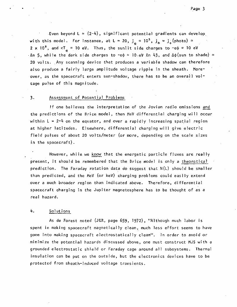
Even beyond L = (2- ), significant potential gradients can develop
with this model. For instance, at L = 20, j = 109, j+ = j. (photo) -
2 x 10⁸, and <T = 10 eV. Thus, the sunlit side charges to -e<j> - 10 eV
Sin 5, while the dark side charges to -e<j> - 10.eV £n k3, and A$(sun to shade) =
20 volts. .Any scanning device that produces a variable shadow can therefore
also produce a fairly large amplitude voltage ripple in the sheath. More-
over, as the spacecraft enters sun-shadow, there has to be an overall vol-
tage pulse of this magnitude.
i •
3. Assessment of Potential Problems
If one believes the interpretation of the Jovian radio emissions and
the predictions of the Brice model, then MeV differential charging w i l l occur
within L = 2-k on the equator, and over a rapidly increasing spatial region
at higher latitudes. Elsewhere, differential charging w i l l give electric
field pulses of about 20 volts/meter (or more, depending on the scale sizes
in the spacecraft).
However, while we know that the energetic particle fluxes are really
present, it should be remembered that the Brice model is only a theoretical
prediction. The Faraday rotation data do suggest that N(l_) should be smaller
than predicted, and the MeV (or keV) charging problems could easily extend
over a much broader region than indicated above. Therefore, differential
spacecraft charging in the Jupiter magnetosphere has to be thought of as a
real hazard.
A. Solutions
As de Forest noted (JGR, page 659, 1972), "Although much labor is
spent in making spacecraft magnetically clean, much less effort seems to have
gone into making spacecraft electrostatically clean". In order to avoid or
minimize the potential hazards discussed above, one must construct MJS with a
grounded electrostatic shield or Faraday cage around all subsystems. Thermal
insulation can be put on the outside, but the electronics devices have to be
protected from sheath-indu-ced voltage transients.

NEGATIVE (ELECTRON) CURRENTS POSITIVE (PROTON AND PHOTOEMISSION) CURRENTS
1010L_
V io8h-(CM2SEC)"]
10C
n l r ' ' ' ' I ' *~j_ ASSOCIATED WITH10 EV ELECTRONS
(BRICE-IOANNIDIS MODEL) "A
j_, AT
EQUATOR
EQ = 6 MEV
j_, RADIATION
WORKSHOP UPPERLIMIT MODEL
I i i i
1010
10*
10C
l T I I i i i i T
j+ASSOCIATED WITH
10 EV PROTONS (BRICE-IOANNIDIS MODEL)
t
AT EQUATOR^
j^ EMISSION OF
PHOTOELECTRONS•FROM ILLUMINATED
SURFACES
/ RADIATION'
WORKSHOP UPPERLIMIT MODEL
i i i i i i I4 6 8 10
JUPITER L-VALUE
20 30 4 6 8 10
JUPITER L-VALUE
20 30
18864-600^-RO-OO
APPENDIX 3
to
FINAL REPORT OF THE OPGT/MJS
PLASMA WAVE SCIENCE TEAM

-.->--: »~-«. f., ,-" fj
'•*./ • 8301-72-86
Bldg R-l, Rm 10705 Kay 1972
Dr. E. J. Smi thSpace Sciences DivisionJet Propulsion LaboratoryIj800 Oak Grove DrivePasadena, California 91109
Dear Ed:
Several people left the May 3 EMC Specification Meeting with very dis-quieting feelings about the s u i t a b i l i t y of using present Mariner orViking spacecraft fabrication techniques without change for the MJSmission. For the past year we have talked about a payload that is abouthalf particles, waves and fields, and this type of payload has beenwidely advertised to SAG, SSB, and others. Yet if MJS is really b u i l twith unshielded boxes and cables, and with minimum or non-existent EMCspecifications on spacecraft subsystems, then modern particle, fieldand wave instruments w i l l not work on the spacecraft. For instance,as discussed at the meeting, energetic particle experiments on Pioneer 9(Webber) and on IMP-6 (McDonald) gave spurious readings in i n i t i a lground tests because of noise on the engineering lines. These problemswere fixed up, and the instruments work perfectly in space. However,IMP and Pioneer, as well as OGO, Injun, Vela, all recent Air Forcespacecraft, etc. are b u i l t to operate with a variety of magnetosphericinstruments, and they all have grounded shields around every electronicsubsystem, power cable, etc.
The argument presented at the meeting (that previous Mariners haven'thad trouble) is really irrelevant. The last Mariner to carry particlesand fields instruments was Mariner 5, and this used rather old experi-ment technology. We are now asking people to draw on recently developedinstrument techniques. I assume that MJS is intended to carry out com-parative Saturn-Jupiter investigations that are at least as sophisticatedas the one now being carried out on Pioneer F,G. Yet all the Pioneer F,Gelectronics is within a shielded container, and all spacecraft subsystemsand cabling are shielded. I doubt very much that any of the four PioneerF,G energetic particle experiments could operate correctly within an opencompartment, with 100 volt peak to peak square waves at 2.4 kHz, and noshielding of any spacecraft subsystems. Of course, many experimentersw i l l propose on the basis of IMP H,I,J technology, and these very moderninstruments w i l l certainly not tolerate the noise environment presentlycontemplated.
SYSTEMS CROUP OF TflW INC. « ONE SPACE PARK. HEDONOO BEACH, CALIFORNIA 90278 • (213) 535-4321
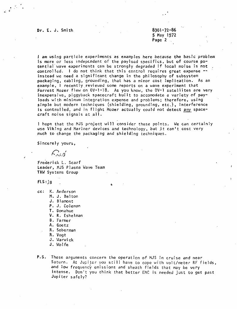
Dr. E. J. Smith 8301-72-865 May 1972Page 2 .
I am using particle experiments as examples here because the basic problemjs more or less independent of the payload specifics, but of course po-tential wave experiments can be strongly degraded if local noise is not .controlled. I do not think that this control requires great expense —instead vie need a significant change in the philosophy of subsystempackaging, cabling, grounding, that has a minor cost implication. As anexample, I recently reviewed some reports on a wave experiment thatForrest Mozer flew on OV-1-18. As you know, the OV-1 satellites are veryinexpensive, piggyback spacecraft built to accomodate a variety of pay-loads with minimum integration expense and problems; therefore, usingsimple but modern techniques (shielding, grounding, etc.), interferenceis controlled, and in flight Mozer actually could not detect ajny_ space-craft noise signals at .all.
1 hope that the MJS project will consider these points. We can certainlyuse Viking and Mariner devices and technology, but .it can't cost verymuch to change the packaging and shielding techniques.
Sincerely yours,
Frederick L. ScarfLeader, MJS Plasma Wave TeamTRW Systems Group
FLS:jg
cc: K. AndersonM. J. Bel tonJ. BlamontP. J. ColemanT. DonahueV. R. EshelmanB. FarmerA. GoetzR. SobermanR. VogtJ. WarwickJ. Wolfe
P.S. These arguments concern the operation of MJS in cruise and nearSaturn. At Jupiter you s t i l l have to cope with volt/meter RF fields,and low frequency emissions and sheath fields that may be veryintense. Don't you think that better EMC is needed just to get pastJupiter safely?
JET PROPULSION LABORATORY
TO: R. L. Heacock
FROM: T. E. Gindorf/J. G. Bastow
SUBJECT: EMC Testing of Viking Hardware in Support of MJS'77
INTEROFFICE MEMORANDUM2946-72-40/2949-72-41
.15 May 1972 .
Some of the field and wave experimenters interested inMJS'77 opportunities have expressed concern about the EMC practicesfollowed on Mariner spacecrafts. If a comparison is nade with otherNASA programs, it is readily apparent that the EMC testing effort ismuch smaller on JPL programs. In the past this effort has beenadequate because the spacecraft have carried a minimum of sensitivewave and field experiments. i
j
Two major problems are created by the Mariner style ofopen subassembly packaging. First, any circuitry or wiring notshielded from the interplanetary plasma results in a coupling ofsignals and noise on the circuit or wire directly into the PlasmaWave/Radio Astronomy E-field antennas. This condition can only beresolved by ensuring that the complete external surface of the spacecraft is a continuous electric shield and that all wires that pene-trate outside this shield are also shielded.
The second problem is the coupling of extraneous signalsand noise between subassemblies within the spacecraft bus eitherdirectly between unshielded sub'systen circuits, or by means ofunshielded or poorly shielded wires and cables. Such interferencecauses a more serious problem to sensitive analog experiments thanit does to engineering subsystems or less sensitive experiments.In the latter cases immunity can be built into the subsystems inmany cases and the level of allowable interference can be quite highif intended signals arc also relatively high (on the order of volts),as is most often the case. This is the philosophical basis forViking conducted noise generation and immunity requirements. Withwave and field experiments, however; all interference is detrimental.Even -though it cannot be completely eliminated, any interferencereduction is beneficial. From a science point of view, significantreduction has been described as essential and has been achieved onother spacecraft, notably I.MP-I.
Although the open style subassembly packaging has beenemployed by JPL for a considerable length of time, most non-JPLspacecraft subsystems (Pioneer, OGO, IMP, etc.) have been completely

R. L. Heacock —2— 2946-72-40/2949/72-4115 May 1972
contained in shielded enclosures. It is impossible to confidentlyestimate the interference generated by Mariner type pubassembliesas virtually no measurements have been made of either the generatedconducted or radiated interference as a function of frequency in theMIL Spec manner since 1963. Consequently, it :Ls currently impossibleto comprehend either what the real adverse effects would be on sensi-tive experiments or to what extent corrective .£MC measures couldeconomically be adapted on JPL spacecraft. It is safe to say that wehave made little real progress with EMC since '..larger and actually areonly scratching the surface in the Viking program. To some extent • /prior spacecraft have not required stringent control because of less *^sensitive experiments or spacecraft subsystems. As a point ofreference, the EMC requirements on the J?L CR3ETER are considerablyless stringent than those being imposed on the MARTIN LANDER. It isunfortunate that progressive design and test improvement has not beenmade in EMC at JPL as has been done with other environmental disciplines.
It is strongly recommended that the MJS'77 project persuadethe Viking Orbiter project to conduct (with assistance as requested),passive EMC measurements on inherited Viking prototype or type approvalhardware at the earliest practical dace. Such measurements could beintegrated into the present more limited Viking subsystem test programwith minimum impact or cost. Such information would serve as a basisfor understanding necessary corrective measures on the MJS'77 and futureprograms and also provide experimenters with information essential toadpatir.g their experiment to the spacecraft environment. This testing,involving about seven subsystems would probably require an additionalday for those subsystems to be EMI tested in-house and two days at JPLfor those to be tested for Viking at contractor facilities. Equipmentand facilities required for these tests are available on Lab. Totaladded cost would be on the order of S20K. These tests would furnishearly information on the adequacy of JPL/Mariner class spacecraft ascompared to the Pioneer spacecraft in providing a suitable platform forfield, particle and wave experiments and indicate the degree of improve-ment necessary in Viking hardware.
JGB/TEG:hem
cc: D. T. Frar.kosM. Frandsen
D. S. KessR. F. DraperW. S. ShipleyE. J. SmithH. M. Schurmeier
/J. G. Bastow/T. .£<" Gindc-rfEnvironmental Requi rements Section
CONFERENCE REPORT
JET PROPULSION LABORATORYREPORT NO..
Page 1 of 3_
SUBJECT Summary of an MJS Electromagnetic Compatibility Meeting
PROJECT MJS1 77 CONTRACTOR CONTRACT or
ACTION REQUIRED BY.
TELECON Initiated by
CONFERENCE at JPL. 183-427
Dote of Occurrence May_3,1972
Report Prepared by A .M.A. Frandsen
Date Prepared 5/15/72
Revised 5/25/72
Participants Distribution
J. G. Bastow,T. N. Divine,R. F. Draper,A. M. A. Frandsen,T. E. Gindorf,D. P. Martin,R. Pelzer,W. Pfeiffer,F. L. Scarf,E. J. Smith,R.. L. Stoller,J. W. Warwick,R. Weber,
JPLJPLJPLJPLJPLJPLU. of Mich.U. of IowaTRWJPLJPLU. of Colo.GSFC
Participants, MJS Plasma Wave Team,MJS Radio Astronomy Team,T. H. Bird, JPLC. B. Farmer, JPLW. G. Fawcett, JPLH. L. Friedman, JPL-J. K. Haas, • JPLR. L. Heacock, JPLM. A. Mitz, NASA HQD. G. Rea, JPLL. L. Simmons, JPLH. M. Schurmeier, JPLF. H. Wright, JPL
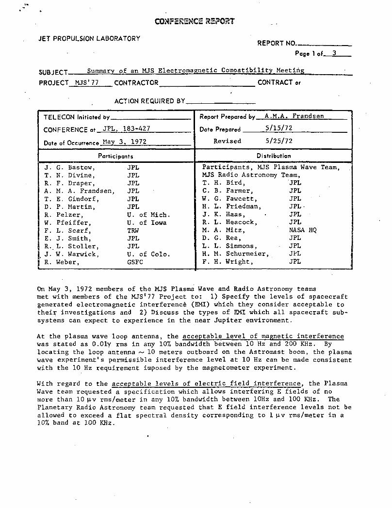
On May 3, 1972 members of the MJS Plasma Wave and Radio Astronomy teamsmet with members of the MJS'77 Project to: 1) Specify the levels of spacecraftgenerated electromagnetic interference (EMI) which they consider acceptable totheir investigations and 2) Discuss the types of EMI which all spacecraft sub-systems can expect to experience in the near Jupiter environment.
At the plasma wave loop antenna, the acceptable level of magnetic interferencewas stated as O.Oly rms in any 10% bandwidth between 10 Hz and 200 KHz. Bylocating the loop antenna ~ 10 meters outboard on the Astromast boom, the plasmawave experiment's permissible interference level at 10 Hz can be made consistentwith the 10 Hz requirement imposed by the magnetometer experiment.
With regard to the acceptable levels of electric field interference, the PlasmaWave team requested a specification which allows interfering E fields of nomore than 10 u-v rms/meter in any 107o bandwidth between lOHz and 100 KHz. ThePlanetary Radio Astronomy team requested that E field interference levels not beallowed to exceed a flat spectral density corresponding to 1 p,v rms/meter in a10% band at 100 KHz.
-2-
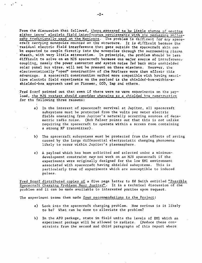
Frora the discussion that folicved, thera appeared to be little chance of age- tineither tear.s' electric field interfqrer.ee requlr_a_mer.ts with theophy traditionally used on the . Marlivsrs. The problem Is difficult for" as y spacc-creft carrying raoncpoles mounted on the structure. It is difficult because tharesidual electric field interference thaz gets outside the spacecraft skin canbe expected to couple directly into the sr.onopoles through the surrounding plasmasheath, with very little attenuation. In principle, the problem should bo. lessdifficult to solve on an HJS spacecraft because ona major source of interferencecoupling, namely the power converter and systsc noise fed back onto unshieldedsolar panel bus wires, will not be present on these missions. However, theelectrostatically "open" construction of the Mariners more than off sate thisadvantage. A spacecraft construction method more compatible with having sensi-tive electric field experiments on the payload is the shielded-bcx-within-a-shielded-box approach used on Pioneer, OGO, Imp and others.
Fred Scarf pointed out that even if there were no wave experiments on the pay-load, the MJS project should consider changing to a shielded box constructi.cnfor the following thrse reasons :
a) In the interest of spacecraft survival at Jupiter, all spacecraftsubsystems must be protected from the volts per meter electricfields emanating from Jupiter's naturally occurring sources of deca-metric radio noise. (Bob Pelzer points out that this is not unlikerequiring the spacecraft to operate within a screen room containinga strong RF transmitter) .
b) The spacecraft subsystems must be protected from the effects of arcingcaused by the large differential electrostatic charging phenomenalikely to occur within Jupiter's plasmasphere .
c) A payload which has been solicited and selected under a minimum-development constraint mayi not work on an MJS spacecraft if theexperiments were originally designed for the low EMI environmentassociated with spacecraft having shielded subsystems. This isparticularly true of experiments which are susceptible to inducedpulses .
Fred Scarf distributed copies of a five page letter to Ed Smith entitled "PossibleSpacecraft Charging Problems Near Jupiter" . It is a technical discussion of theproblem and it can be made available to interested parties upon request.
The experiment teams then made four recommendations to the Project;
a) 'Look into the spacecraft charging problem. How serious is it likelyto be? What can be done to alleviate the problem?
b) In the AFO package, state in field units the levels of EMI which anexperiment package will be allowed to radiate. (Deduce these con-straints from the second and third paragraphs of this report where
-3-
the acceptable levels of interference at the wave experimenters'antennas are given). Also include in .the AFO package a constrainton the maximum allowable conducted interference which can be gen-erated on experiment interface lines, namely 30 mv.
c) Consider changing the subsystem packaging and bonding philosophiesso that each subsystem represents an enclosed conducting box.Consider changing the shielding philosophy so that a shield surround-ing an inter-subsystem wire bundle is an extension of both subsystems'chassis - even through a connector, where the connector shell is alsopart of the shield envelope. Consider tight twisting and doubleshielding of the 50 volt AC power distribution lines within the space-craft. ,
d) As soon as it becomes practical, measure the radiated and conductedinterference levels associated with Viking hardware. After theseresults are evaluated, and prior to the issuance of a spacecraftsystem RFP, negotiate with the selected payload experimenters toestablish the final EMI constraints that will apply to both instru-ments and subsystems.

1886A-60Q1»-RO-00
APPENDIX k
to
FINAL REPORT OF THE OPGT/MJS
PLASMA WAVE SCIENCE TEAM

PLASMA WAVE TEAM ORGANIZATION AND EXPERIENCE
TEAM MEMBERS SUCCESSFUL S/C LAUNCHES(WAVE EXPERIMENTS)
PENDING LAUNCHES
F. SCARF -
TRW SYSTEMS GROUP
, OV3-3
PIONEER 8
PIONEER 9
OGO-5
IMP-H
ATS-G (?)
D. GURNETT
UNIVERSITY OF IOWA
INJUN 3, INJUN 5
IMP-6, S3-A
IMP-J, HELIOS A,
HELIOS B, INJUN F,
ATS-G (?)
R. HELLIWELL
STANFORD UNIVERSITY
OGO-1 , OGO-2, OGO-3
OGO-4, OGO-6
E. SMITH, A. FRANDSEN
JET PROPULSION LAB
R. HOLZER
UCLA
P. KELLOGG
UN IV OF MINNESOTA
OGO-1, OGO-2, OGO-3
OGO-4, OGO-5, OGO-6
IMP-6 HELIOS A, HELIOS B
E. UNGSTRUP
DANISH SPACE RESEARCH
CENTER
HEOS A2 GEOS
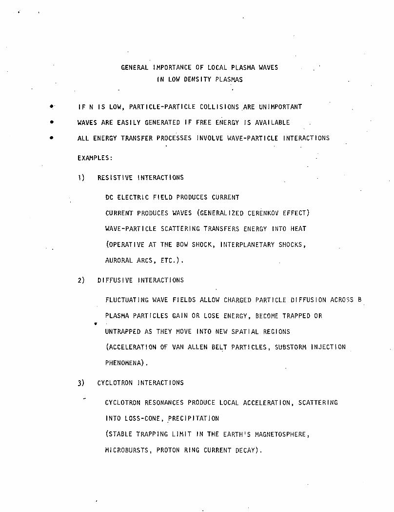
GENERAL IMPORTANCE OF LOCAL PLASMA WAVES - . 'IN LOW DENSITY PLASMAS
• IF N IS LOW, PARTICLE-PARTICLE COLLISIONS .ARE UNIMPORTANT
• WAVES ARE EASILY GENERATED IF FREE ENERGY IS AVAILABLE
• ALL ENERGY TRANSFER PROCESSES INVOLVE WAVE-PARTICLE INTERACTIONS
EXAMPLES:
1) RESISTIVE INTERACTIONS
DC ELECTRIC FIELD PRODUCES CURRENT
CURRENT PRODUCES WAVES (GENERALIZED CERENKOV EFFECT)
WAVE-PARTICLE SCATTERING TRANSFERS ENERGY INTO HEAT
(OPERATIVE AT THE BOW SHOCK, INTERPLANETARY SHOCKS,
AURORAL ARCS, ETC.).
2) DIFFUSIVE INTERACTIONS
FLUCTUATING WAVE FIELDS ALLOW CHARGED PARTICLE DIFFUSION ACROSS B
PLASMA PARTICLES GAIN OR LOSE ENERGY, BECOME TRAPPED OR«
UNTRAPPED AS THEY MOVE INTO NEW SPATIAL REGIONS
(ACCELERATION OF VAN ALLEN BELT PARTICLES, SUBSTORM INJECTION
PHENOMENA).
3) CYCLOTRON INTERACTIONS
CYCLOTRON RESONANCES PRODUCE LOCAL ACCELERATION, SCATTERING
INTO LOSS-CONE, PRECIPITATION
(STABLE TRAPPING LIMIT IN THE EARTH'S MAGNETOSPHERE,
MICROBURSTS, PROTON RING CURRENT DECAY).

THE ROLE OF PLASMA WAVE MEASUREMENTS FOR MJS
1. ORIGIN AND DYNAMICS OF THE JUPITER RADIATION BELTS
(SUMMARY OF RADIATION WORKSHOP MODELS)
HUGE ROTATION SPEED GIVES A MAGNETOSPHERE BOUNDARYTHAT IS "POROUS"
BOW SHOCKAT 70 R.
JUPITER
SOLAR WIND
ELECTROSTATIC WAVES ATTHE "BOW SHOCK CAUSE RE-SISTIVE PARTICLE HEATINGTHERE ARE JUMPS IN(<T/B) TO ABOUT 100 MeV/GAUSS
VARIOUS WAVESALLOW INWARDDIFFUSION WITHCONSERVATION OF
ION AND ELECTRON CYCLOTRONMODE TURBULENCE DEVELOPSFOR T > 1,, . PARTICLES
> B2/8fTN ARE SCATTERED
'AWITH EAND THE STABLYIS LIMITED
TRAPPED FLUX
2. OTHER ASPECTS OF PARTICLE-PLASMA WAVE INTERACTIONS AT JUPITER
'CYCLOTRON RESONANT INTERACTIONS CAN LOCALLY ACCELERATE PAR-TICLES, IN ADDITION TO CAUSING PRECIPITATION AND DIFFUSION.
WE KNOW THAT NEAR THE EARTH, ELECTROSTATIC WAVES ARE MOSTEFFICIENT IN CAUSING SCATTERING, BUT THE RADIATION WORKSHOPMODELS IGNORE THESE MODES.
THE 10-MODULATION OF THE DECAMETER RADIATION IS COMMONLY IN-TERPRETED IN TERMS OF PHENOMENA INVOLVING LOCAL PLASMAWAVES (SUCH AS TURBULENT RESISTIVITY). MILLISECOND MODU-LATION IS DETECTABLE AT EARTH.
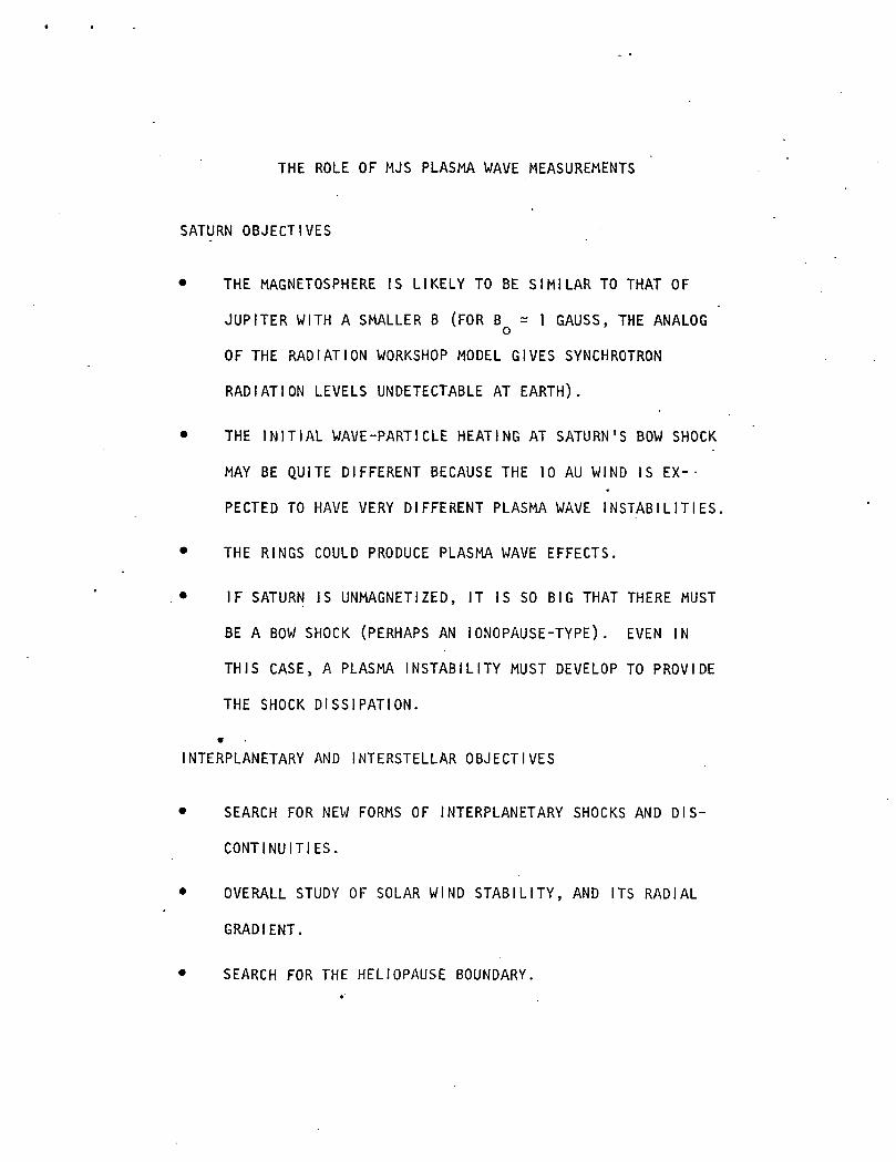
THE ROLE OF MJS PLASMA WAVE MEASUREMENTS
SATURN OBJECTIVES
• THE MAGNETOSPHERE IS LIKELY TO BE SIMILAR TO THAT OF
JUPITER WITH A SMALLER B (FOR B = 1 GAUSS, THE ANALOGo
OF THE RADIATION WORKSHOP MODEL GIVES SYNCHROTRON
RADIATION LEVELS UNDETECTABLE AT EARTH).
• THE INITIAL WAVE-PARTICLE HEATING AT SATURN'S BOW SHOCK
MAY BE QUITE DIFFERENT BECAUSE THE 10 AU WIND IS EX--
PECTED TO HAVE VERY DIFFERENT PLASMA WAVE INSTABILITIES.
• THE RINGS COULD PRODUCE PLASMA WAVE EFFECTS.
• IF SATURN IS UNMAGNETIZED, IT IS SO BIG THAT THERE MUST
BE A BOW SHOCK (PERHAPS AN IONOPAUSE-TYPE). EVEN IN
THIS CASE, A PLASMA INSTABILITY MUST DEVELOP TO PROVIDE
THE SHOCK DISSIPATION.
*
INTERPLANETARY AND INTERSTELLAR OBJECTIVES
• SEARCH FOR NEW FORMS OF INTERPLANETARY SHOCKS AND DIS-
CONTINUITIES.
• OVERALL STUDY OF SOLAR WIND STABILITY, AND ITS RADIAL
GRADIENT.
• SEARCH FOR THE HELIOPAUSE BOUNDARY.
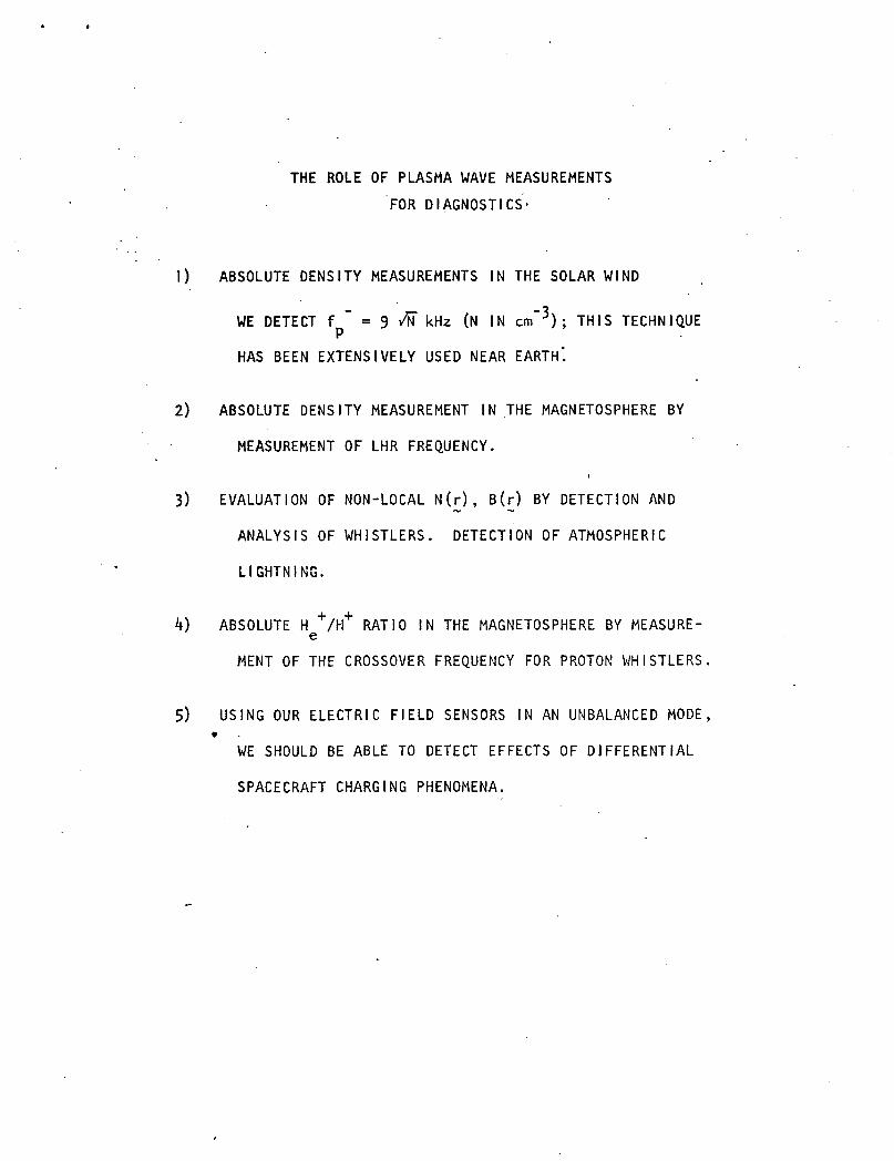
THE ROLE OF PLASMA WAVE MEASUREMENTS
FOR DIAGNOSTICS-
1) ABSOLUTE DENSITY MEASUREMENTS IN THE SOLAR WIND
WE DETECT f " = 9 v¥ kHz (N IN cm"3); THIS TECHNIQUE
HAS BEEN EXTENSIVELY USED NEAR EARTH*.
2) ABSOLUTE DENSITY MEASUREMENT IN THE MAGNETOSPHERE BY
MEASUREMENT OF LHR FREQUENCY.
3) EVALUATION OF NON-LOCAL N(r), B(r) BY DETECTION AND
ANALYSIS OF WHISTLERS. DETECTION OF ATMOSPHERIC
LIGHTNING.
ABSOLUTE H +/H+ RATIO IN THE MAGNETOSPHERE BY MEASURE-
MENT OF THE CROSSOVER FREQUENCY FOR PROTON WHISTLERS
5) USING OUR ELECTRIC FIELD SENSORS IN AN UNBALANCED MODE,•
WE SHOULD BE ABLE TO DETECT EFFECTS OF DIFFERENTIAL
SPACECRAFT CHARGING PHENOMENA.

MJS PLASMA WAVE INSTRUMENT
MEASUREMENTS
HIGH TIME RESOLUTION BANDPASS CHANNELS .
32-CHANNEL SPECTRUM ANALYZER (20 Hz-200,000 Hz)CONTINUOUS AVERAGE READINGSPEAK SAMPLE AND HOLD FOR IMPULSESSWITCH FROM E TO B
WAVEFORM (ASSUMES 10 kb BUFFER)
10 TO 300 Hz E OR B WAVEFORMSCAPTURE 1 SEC SNAPSHOTS AND READ OUT.
PLASMA WAVELOOP ANTENNA
MAGNETOMETEi
15.2m BOOM
-RAD!0 ASTRONOMY/PLASMA WAVE DETECTORS^Om)

U
z
ENCELADUS
MIMAS
1 - r
10'
10C
i - 1 - 1 - 1: 32-CHANNEL
SPECTRUM ANALYZER,. PEAK AND AVERAGE
io
10 r
TETHYS
DIONE
RHEA
SATURN
B S ( L = 1) = 1 GAUSS
N$(L) = 0.25Nj(L)
0 20 40 \ 1
ATTENUATION, db WAVEFORM
AMALTHEA IO EUROPA GANYMEDE
JUPITER
Bj (L=l)= 10 GAUSS
Nj (L) GIVEN BY
BRICE-IOANNIDISMODEL
11 , 13 15

32 -CHANNELSPECTRUM ANALYZER,PEAK AND AVERAGES
106F
105 r
(Hz)
10"
10 I
EARTH
20 40
ATTENUATION, db WAVEFORM
WAVE MODES IN THE SOLAR WIND,AT THE PLAN ETARY BOW SHOCKS,AND IN THE PLANETARY MAGNETOSHEATHSOR IONOSHEATHS
EXTENDED MISSION

MISSION REQUIREMENTS
WEIGHT: k.O IBS + SENSORS. POWER: 2.0 WATTS
SENSORS: WE MUST HAVE AN ELECTRIC DIPOLE; THE MAGNETIC SENSOR
IS A VITAL BACKUP.
TM: WE WANT SEVERAL HUNDRED BITS/SEC AT ENCOUNTER TO
OBTAIN THE NECESSARY HIGH TIME RESOLUTION.
BUFFER: WE PROPOSE TO CAPTURE AUDIO FREQUENCY (10 TO 300 Hz)
WAVEFORMS THROUGHOUT THE MISSION USING A 10 kb BUFFER.
EMC CONSIDERATIONS
MARINER FACES SEVERE ELECTRICAL HAZARDS PASSING JUPITER:
• IT IS KNOWN THAT THERE WILL BE AMBIENT RF FIELDS WITH VOLT/
METER AMPLITUDES.
• THERE WILL BE VLF FIELDS WITH UNDETERMINED AMPLITUDES (NO
PIONEER F,G DATA).
• THERE CAN BE SEVERE SPACECRAFT CHARGING PROBLEMS (ATS-5 AND
OTHER SPACECRAFT DETECT 300 V/M TO 3 keV/METER LOCAL E-FIELDS
IN REGIONS OF EARTH ORBIT WHERE KT * 5 TO 20 keV; THE6
JOVIAN BELTS HAVE HUNDREDS OF keV TO MeV THERMAL ENERGIES).
MEASURES MUST BE TAKEN TO PROTECT MARINER SUBSYSTEMS FROM THESE
HAZARDS (ELECTRICAL SHIELDING OF THE ENTIRE SPACECRAFT, OF ALL
CABLES, OF ALL SUBSYSTEMS).
THESE SAME MEASURES WILL AUTOMATICALLY SOLVE THE POTENTIAL PLASMA
WAVE EMC PROBLEMS (THE ABSENCE OF SOLAR PANELS IS A GREAT HELP
IN THIS AREA; THESE PANELS HAVE ALWAYS BEEN A MAJOR SOURCE OF NOISE)
I8864-600A-RO-00
APPENDIX 5
to
FINAL REPORT OF THE OPGT/MJS
PLASMA WAVE SCIENCE TEAM

Plasma Wave Experiment for OPGT
byR. L. Smith and R. A. Helliwell
July 1972
Final Report
Prepared under
TRW Systems GroupSubcontract 105GB1-SC
wn^Fn'III n.1 UM f m
PLASMA WAVE EXPERIMENT FOR OPGT
R. L. Smith and R. A. HelliwellRadioscience Laboratory
Stanford UniversityStanford.California
Final Report
Prepared Under
TRW Systems GroupSubcontract 105GB1-SC
July 1972

CONTENTS
Page
LOW-NOISE PREAMPLIFIERS 1
MULTI-COUPLERS 3
PRACTICAL SENSITIVITIES 4
SUGGESTED INTERFERENCE SPECIFICATIONS 6
SPACECRAFT SYSTEM INTERFERENCE SOURCES 10
GROUP INTERFACES 11
RADIO ASTRONOMY INTERFACE 12
1. Orientation of Electric Antenna 12
2. Feed Point of Electric Antenna 13i
DUAL SWEEPING EXPERIMENT 14
LOGARITHMIC SWEEPING RECEIVER 14
REFERENCES . , , '................ 16
iii

ILLUSTRATIONS
Characteristics of minimum detectable signals 2
2 Sensitivities of EOGO, POGO, and a possible OPGT vlfsystem of magnetic field detectors, compared to currentOPGT interference specifications 5
3 Electric field sensitivities, OGO-III, based on laboratoryand inflight measurements 7
4 Maximum allowable dynamic magnetic field at one meterdue to a subsystem 8
5 Maximum allowable generated electric field inter-ference levels 9
iv

PLASMA WAVE EXPERIMENT FOR OPGT
R. L. Smith and R. A. HelliwellRadioscience LaboratoryStanford UniversityStanford,California
This report deals with the proposed plasma wave experiment for
the Outer Planets Grand Tour (OPGT). The emphasis is on sensitive
receivers for the detection of magnetic and electric fields at very
low frequencies, interference specifications, interference reduction,
and interfaces with other experiments.
The results of .our study reflect previous experience on five OGO
spacecraft, and a previous proposal to measure electric and magnetic
fields on the Jupiter mission (Pioneers F and G). Substantial parts
of this report are based on work growing out of a meeting of R. L.
Smith and Al Frandsen with L. H- Rorden of DeveVo, inc. Mr. Rorden.
was the design engineer for four of the Stanford University/Stanford
Research Institute vlf experiments on OGO, and also participated in
the Jupiter mission proposal.
We first give a short discussion on available sensitivities of
magnetic and electric sensors to form a basis for some of the later
suggestions. A section on practical measured and predicted sensi-
tivities follows. A number of specific suggestions are made for
reducing interference. The problems of interfacing to related experi-
ments are reviewed . A possible plasma wave experiment is then briefly
discussed.

LOW-NOISE PREAMPLIFIERS
An excellent discussion of low noise broadband vlf receiving tech-
niques is given by Rorden [1965]. The fundamental limitations are the
noise temperature of the preamplifier, the "effective volume" of the
antenna, the antenna bandwidth and the desired frequency and system
bandwidth. The effective volume of a dipole is approximately
dip ~ Loga/a)-l
where £ is the half length and "a" the wire radius. The effective
volume of a single turn loop is
2K3_ Jt D
loop Log(b/a)
where "b" is the loop radius, and "a" the wire radius. The antenna
bandwidth in radians per second is given by
"dip = G/C
0,loop
for the dipole and loop, respectively, where G is the parallel con-
ductance of a dipole with an effective capacitance C, and R is the
series resistance of a loop with inductance L. These quantities are
functions of the antenna geometry, size, and the amount of conducting
material (mass). The effective volume, antenna bandwidth and preamplifier
noise temperature set a lower limit on the minimum detectable power in a
unit bandwidth at a.given frequency for a narrowband system. Generally
this curve has a slope of -2 with frequency (in log coordinates) as
- 1 -
watts/Hz
10 dB
a,b
0,01 f 0,1 f, 10 f, 100 f.
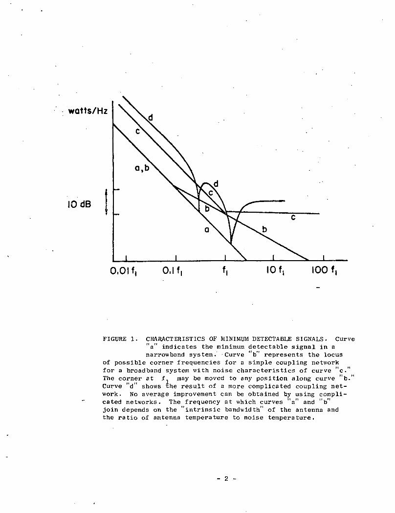
FIGURE 1. CHARACTERISTICS OF MINIMUM DETECTABLE SIGNALS. Curve"a" indicates the minimum detectable signal in anarrowband system. Curve "b" represents the locus
of possible corner frequencies for a simple coupling networkfor a broadband system with noise characteristics of curve "c."The corner at f.. may be moved to any position along curve "b."Curve "d" shows the result of a more complicated coupling net-work. No average improvement can be obtained by using compli-cated networks. The frequency at which curves "a" and "b"join depends on the "intrinsic bandwidth" of the antenna andthe ratio of antenna temperature to noise temperature.
- 2 -

shown schematically by curve "a" in Figure 1.
The variation of minimum detectable signal with frequency for a
broadband system depends on the nature of the coupling network between
the antenna and preamplifier. For a simple coupling network, responses
of the type indicated by curve "c" can be obtained, where the best
obtainable noise performance can be specified at only one frequency.
More complicated networks can be used to improve the noise performance
in certain frequency ranges, but only at the expense of performance in
other frequency ranges. This is illustrated by curve "d." Note that
the frequency response gain characteristics can be obtained independently
of the noise sensitivity response.
MULTI-COUPLERS
When broadband systems are contemplated for highly reactive sources
(i.e., the problem at hand for either loops or dipoles for antenna sizes
much less than a wavelength), one might be inclined to use a set of pre-
amplifiers with multi-coupler elements added between the source and each
amplifier. Although this problem has not received the consideration it
deserves, the result of some thought and lack of any supportable counter-
proposals indicates that the signal-to-noise ratio can only be degraded
over that of a single amplifier by such an arrangement. The only advan-
tages appear to be redundancy, wherein if one preamplifier fails, the
other(s) might continue to work, and reduction of exposure to inter-
modulation distortion from strong signals widely separated in frequency.
A noiseless active filter in the multi-coupler would work if one were
available, but in that case the fictitious noiseless active element could
just as well serve as the amplifier.
- 3 -

An improvement can be obtained by using separate antennas and
amplifier systems, provided they are uncoupled. An alternative scheme
would be to physically switch preamplifier coupling networks sequentially.
PRACTICAL SENSITIVITIES
It is reasonable to base the estimated sensitivities of inter-
planetary probes on prior satellites, such as EOGO's which have penetrated
this space at least locally. The principles discussed above were used
in the design of the Stanford University/Stanford Research Institute vlf
magnetic receivers for the EOGO and POGO spacecraft. The effective
volume of the OGO antennas is roughly 5 cubic meters. This may be
compared with a possible OPGT antenna in the form,of a rectangle 6 ft.
by 6 in., using 1/4 kg of copper, which has an effective volume of
0.03 cubic meters, a loss of 22 db with respect to OGO. The frequency
of optimum sensitivity for EOGO was set at 100 kHz, and that for POGO at
10 kHz. Thus the theoretical low frequency sensitivity of POGO is about
10 db better than that of EOGO. At 200 Hz the measured sensitivities
/ 1/2were -106 db and -88 db with respect to IY/HZ • If we assume that
the OPGT coupling network will have a corner frequency at 3 kHz, the
sensitivity will be comparable to EOGO below that frequency. At an
assumed upper frequency limit of 15 kHz, the performance will be degraded
from EOGO by 14 db. These various sensitivities are illustrated in
Figure 2.
The laboratory measurements of the electric field sensitivities of
OGO-3, assuming an effective length equal to half the length from boom
1/2tip to boom tip varies from -36 db to -53 db with respect to lu.V/m/Hz '
over the frequency range from 200 Hz to 100 kHz. This assumes that the
- 4 -

dB BELOWlr/H2l/2
-40
-60
-80
-100
-120
-140
-160
-180
CURRENT OPGTINTERFERENCE SPECIFICATION
10 Hz 100 Hz kHz 10 kHz 100 kHz
FIGURE 2. SENSITIVITIES OF EOGO, POGO, AND A POSSIBLEOPGT VLF SYSTEM OF MAGNETIC FIELD DETECTORS,COMPARED TO CURRENT OPGT INTERFERENCESPECIFICATIONS.
- 5 -

antenna impedance is small compared to the input impedance. Laboratory
measurements and typical in-flight noise measurements are shown in
Figure 3.
SUGGESTED INTERFERENCE SPECIFICATIONS
It is somewhat difficult to translate the above figures into
interference specifications of the type given in the OPGT tables because
certain assumptions must be made regarding the nature of the interference.
The most severe assumption is that the interference may be radiated with
an intensity varying as inverse distance from, say, the main body. A
somewhat relaxed assumption is an inverse square or inverse cube law.
Probably the simplest approach is to assume that the sensors (antennas)
will be placed one meter from the main body and use the OGO figures
directly. If the sensors are placed further from the interference points,
the values can be relaxed. If we assume an inverse cube variation, the
equivalent interference can be increased by 18 db for each factor of 2
of the spacing of the sensors from the interference points. No OPGT
specifications are indicated for electric fields in Figure 3 because
the current existing specification is being rewritten.
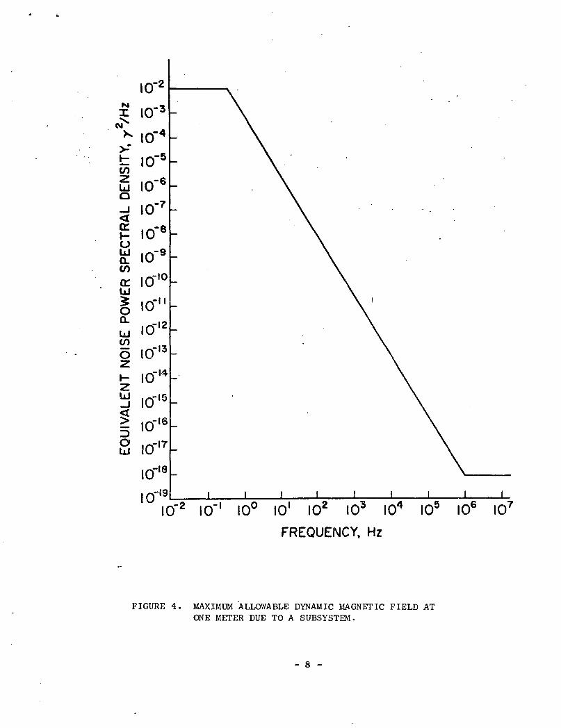
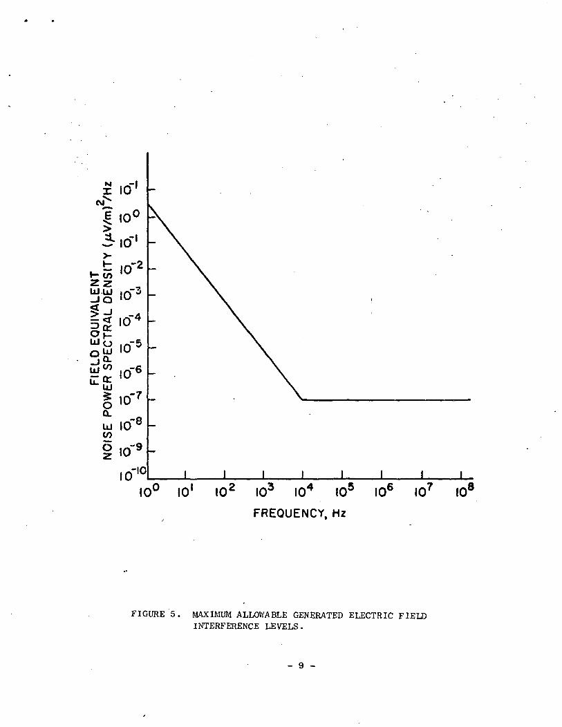
A suggestion is made in Figures 4 and 5 for the maximum inter-
ference levels that should be permitted at the OPGT vlf experiment. In
deriving these curves, the following assumptions were made: 1) The OPGT
spacecraft will be no noisier than the OGO series. 2) For the magnetic
levels, the same values were used below 30 Hz as given in the OPGT
tables. The straight line approximation was continued for higher
— 1 S 2frequencies to a level of 10 y /Hz. This corresponds quite closely
to the best obtainable OGO performance. 3) The levels of magnetic and
- 6 -

dB(/-LV/m/Hzl/2)
+60
+40
+20
0
-20
-40
-60
100 I kHz 10 kHz 100 kHz
FIGURE 3. ELECTRIC FIELD SENSITIVITIES, OGO-III, BASED ONLABORATORY AND INFLIGHT MEASUREMENTS. The laboratorymeasurement assumed a low antenna impedance.
- 7 -
N
10 10° 10° 10'FREQUENCY, Hz
FIGURE 4. MAXIMUM ALLOWABLE DYNAMIC MAGNETIC FIELD ATONE METER DUE TO A SUBSYSTEM.
- 8 -
£ 10f
*-;>-
i-w l0"22zUJui ,n-3-JO IU
Ig l0"4
oUJ l0"5
g« '0«UJ
gio'7(L
UJ IO"8tni io'9
IO'10 _LI01 I02 I03 10' 10' 10' 108
FREQUENCY, Hz
FIGURE 5. MAXIMUM ALLOWABLE GENERATED ELECTRIC FIELDINTERFERENCE LEVELS.
- 9 -

electric fields at 10 MHz correspond to the needs of the Radio Astronomy
experiment.
SPACECRAFT SYSTEM INTERFERENCE SOURCES
Previous experience has shown that major interference sources
frequently are part of the spacecraft system, especially in the power
supply inverters with their associated ripple filters, and in the solar
panels. Proper design and specifications can result in a low noise
spacecraft. It is important to consider the noise problems before the
spacecraft design becomes "frozen."
A common source of a-c magnetic interference is the ripple filter,
not the inverter proper. Three specific recommendations can be made as
follows:
1. Use as high an inverter frequency as possible.
2. The ripple filter toroid must be wound uniformly. This isfrequently not done, with the result that very large dipolemoments remain. The toroids must not be "scramble wound."
3. An eddy current shield should be made as small as possible,surrounding only the coils &nd transformers, not the othercomponents. Walls of the shields should have a continuouslarge cross section. Fasteners, joints, etc., should beeliminated to whatever extent is feasible.
Although solar cells are not planned for OPGT, it is worth noting
that there are various ways in which solar cells may cause trouble, both
in planned and unplanned ways. However a great deal of trouble can be
avoided if the solar cell is designed to trickle charge the battery.
It is vital that all exposed potential surfaces, especially those with
positive potential, be thoroughly insulated. The wires to the solar
cells should be arranged -to minimize loop paths. Note that voltage
regulation does not of itself solve interference problems since noise
currents will frequently show up as voltages on the solar array.
- 10 -

Each wire should be treated as a source of electric and magnetic
fields. The most important wires are those which penetrate the basic
spacecraft skin. Wherever possible the wires penetrating the skin should
be shielded with the shield bonded to the skin as close as possible to
the point of penetration.
GROUP INTERFACES
Meeting the scientific objectives through the design of an optimum
set of experiments will require the cooperation of the various scientific
groups. At this point the two other groups which will have the greatest
influence on the Plasma Wave experiment design are the Magnetic Fields
group and the Radio Astronomy group. One approach is to arrange joint
meetings among members of each of the three groups (the above, plus
Plasma Wave) to discuss detailed scientific problems and possible
engineering compromises. Some areas of common interest are discussed
below.
We are, of course, naturally concerned about possible sources of
interference to the wave experiments. If, as now seems likely, the
magnetic field antenna for the plasma wave experiment will be close to
the magnetometer, the magnetometer becomes the most probably source of
interference. The type of magnetometer chosen should produce negligible
a-c fields. Flux-gate magnetometers are particularly prone to give
interference.
On the other hand we must be concerned with sources of static
magnetic interference to the magnetometer. We need to know in some
detail the sensitivity of the magnetometer. One possible interference
source is the input transformer from the magnetic loop antenna. The
- 11 -
size of the transformer is inversely related to the low frequency cutoff
desired. If the magnetometer is sensitive to a-c magnetic fields, to a
sufficiently high frequency (say, at least 100 Hz), the a-c components
of the magnetometer could be coupled to the plasma wave instrument for
further processing, while the low frequency cutoff of the a-c loop could
be raised, thus reducing the size of the input transformer and consequent
magnetic interference.
RADIO ASTRONOMY INTERFACE
The importance of the electric antenna to the plasma wave experiment
is emphasized in report PW 4 in which it was concluded that "in a truly
minimum plasma wave experiment, electric field measurements would take
precedence over magnetic field measurements." Hopefully any differences
of opinion between the Plasma Wave and Radio Astronomy Groups can be
resolved so that a coordinated and readily defendable proposal can be
made.
Orientation of electric antenna. According to the latest available
information, TOPS configuration 3A, the electric antennas will be oriented
approximately along ±45 lines relative to the x and y axis. Since
a major objective of the Radio Astronomy group is to measure wave polariza-
tion, the symmetry of the antenna system should be examined. The most
obvious source of asymmetry is the 50 ft. magnetometer boom in the -y
direction. The parasitic nature of the boom will cause coupling between
the two antennas. It is not clear that the presence of this boom has been
taken into account as a parasitic element. It could have a considerable
effect on polarization measurements.
The most sensitive arrangement is to operate a monopole antenna in
- 12 -

the +y direction opposite the long boom. In this way the remainder of
the spacecraft becomes in essence the other part of an unbalanced dipole,
with an effective length half the distance from end to end. The other
antenna system would be in the ±x direction. This orientation would
probably interfere with the numerous optical experiments presently placed
opposite the boom. This possibility could nevertheless be examined for
other possible spacecraft.
Feed point of electric antennas. The overall signal-to-inteference
ratio of an electric antenna depends on the location of the feed point.
The principal source of interference is presumably other experiments and
-spacecraft functions. Except for radiation from large objects, like
solar panels, the source size may be considered small compared with
antenna dimensions (assuming a large antenna appropriate to radio astron-
omy) . In a balanced configuration the signal strength v/ill fall roughly
linearly as the feed point is moved outward, but the interference signal
strength should be reduced at a higher inverse power of feed point dis-
tance. This implies that an optimum feed point exists which is neither
at the antenna tip nor at the satellite base connection. The optimum
point of feeding may not be known but can perhaps be estimated using
assumed interference sources. Since we propose to share electric antennas
with the Radio Astronomy group, the input interface becomes vital. As
discussed previously, the maximum sensitivity is obtained by having a
single preamplifier for each sensor. A multi-coupler may be used after
the preamplifier to give the appropriate frequency band to each experiment.
When a single sensor is used over a wide frequency range, the signal-to-
noise ratio will be degraded in some frequency bands (see the section on
low noise preamplifiers).
- 13 -
The frequency band from 15 kHz to 100 kHz is important because of
high-pass noise, band-limited noise, and type III solar noise bursts.
According to the present plan, this frequency range will be covered by
the radio astronomy portion of the experiment. If there is any possi-
bility that this band will not be covered by the Radio Astronomy group,
we must be informed in sufficient time to be able to propose that it be
covered by the Plasma Wave group.
DUAL SWEEPING EXPERIMENT
One interesting possibility for an experiment utilizing multiple
antennas, say two dipoles and a loop, is to use two sweeping receivers
with switchable preamplifiers. The following options are then available:
1. Measure electric and magnetic fields simultaneously.
2. Measure electric field polarization.
3. Measure the dispersive characteristics of electric fieldsignals using offset sweeping of the receivers.
4. Measure the dispersive characteristics of magnetic fieldsignals.
5. Provide redundancy in case one system fails.
Such a system can be built using two bands for each receiver, covering
say 20 to 800 Hz with a 12 Hz bandwidth and 800 to 14,000 Hz with a 200 Hz
bandwidth. The main body package of EOGO, designed 10 years ago, weighed
only 800 gms (1.75 Ibs.) and used less than 1 watt of power. It is,
therefore, likely that such a system described above could be built
within the weight and power limitations of the OPGT. Such a system
would require adding only a preamplifier to the circuitry suggested by
Frandsen and Martin [1971].
LOGARITHMIC SWEEPING RECEIVER
In the normal mode of operation of sweeping receivers an equal
- 14 -

amount of time is spent on each frequency interval, or else certain
frequencies are skipped. As a general principle, it would appear more
useful to be able to frequency-scan in logarithmic increments with
logarithmic bandwidths. The first approximation to this principle is
to use multiple sweeping receivers, as in the OGO series, for example.
There is another possibility that may be used in low data rate
systems. Suppose the rate of frequency stepping is controlled in a
quantized nearly logarithmic fashion by suitable feedback around the
digital frequency control circuits. The highest stepping rate occurs
at some multiple of the data rate, but all frequencies are covered. The
'amplitude of the detected outputs is summed, even though a range of
frequencies may be covered, and the output is read out, then reset, at
each major data cycle. The effect is then quite similar to the use of
multiple filters with logarithmic bandwidths and frequency separations.
If more frequency resolution is required, the receiver can be readily
commanded, or internally controlled, to resume a linear sweep.
- 15 -
REFERENCES
Fraadsen, A. M. A. and D. P. Martin, Preliminary minimum experiment
description (instrument portion only) for the combined OPGT
Plasma Wave and Planetary Radio Astronomy Experiments,
November 19, 1971.
Rorden, L. H., A study of low-noise broadband vlf receiving techniques,
Tech. Rept., Stanford Research Institute, Menlo Park, Calif.,
November 1965.
- 16 -