---

—.-

FINAL REPORT:

Development of a UAV-Mounted 95 GHz Radar Systemto Conduct Scientific Studies of Clouds

DOE Grant: DE-FG02-95ER62023

R.E. McIntosh, Principal Investigator

University of Massachusetts

Microwave Remote Sensing Laboratory

Amherst, MA 01003

Submitted to

Department of Energy

May 16, 2000

Wehave~no0$jection from 8 patentstandpoint to the pubIicat20n ordisseminak$on of this material.

w CbwzVL &f g,~Office of Intellectual

1 DakeProperty Counsel.DOEField Office, Chicago

‘k

DISCLAIMER

This repon was prepared as an account of work sponsoredbyanagency~f the United States Government. Neitherthe United States Government nor any agency thereof, norany of their employees, make any warranty, express orimplied, or assumes any legal liability or responsibility forthe accuracy, completeness, or usefulness of anyinformation, apparatus, product, or process disclosed, orrepresents that its use would not infringe privately ownedrights. Reference herein to any specific commercialproduct, process, or service by trade name, trademark,manufacturer, or otherwise does not necessarily constituteor imply its endorsement, recommendation, or favoring bythe United States Government or any agency thereof. Theviews and opinions of authors expressed herein do notnecessarily state or reflect those of the United StatesGovernment or any agency thereof.

DISCLAIMER

Portions of this document may be illegiblein electronic image products. Images areproduced from the best available originaldocument.

1. INTRODUCTION

This report describes the development and testing of the Compact Millimeter-Wave

Radar (CMR). CMR is a solid-state W-band radar designed for integration on the Depart-

ment of Engergy’s (DOE’s) Atmospheric Radiation Measurement (ARM) Unmanned Aerial

Vehicle (UAV) platforms. One of the primary scientific objectives of the DOE ARM-UAV

program was to investigate the role of clouds in the Earth’s atmospheric radiation balance.

W-band radars have the ability to profile a wide variety of clouds, including ones with high

optical extinction. The DOE ARM-UAV program funded UMass to investigate whether the

size, weight and power consumption of typical airborne W-band radars could be reduce to

meet the constraints imposed by the UAV payload capacity, and based on the results of

this study, funded UMass to build the CMR. In the sections to follow, the design and de-

velopment of the CMR will be described, results from comparisons between CMR and the

UMass Cloud Profiling Radar System (CPRS) presented and upgrades that will enhance the

sensitivity of CMR by 20 dB discussed.

2. Publications

Based on the work. performed for this grant, Dr. Ray Bambha received his PhD from

UMass in 1999. Publications describing this work are listed below:

●

●

Bambha, R.P, “A Compact Millimeter-wave Radar for Studies of Clouds and Precipi-

tation”, PhD Thesis, University of Massachusetts, 1999.

Bambha, R.P., J.R. Carswell, J.B. Mead, and R.E. McIntosh,” A Compact Millimeter

Wave Radar for Airborne Studies of Clouds and Precipitation”, IEEE Geosciencead

Remote Sensing Symposium, Seattle, WA, 1998.

‘2

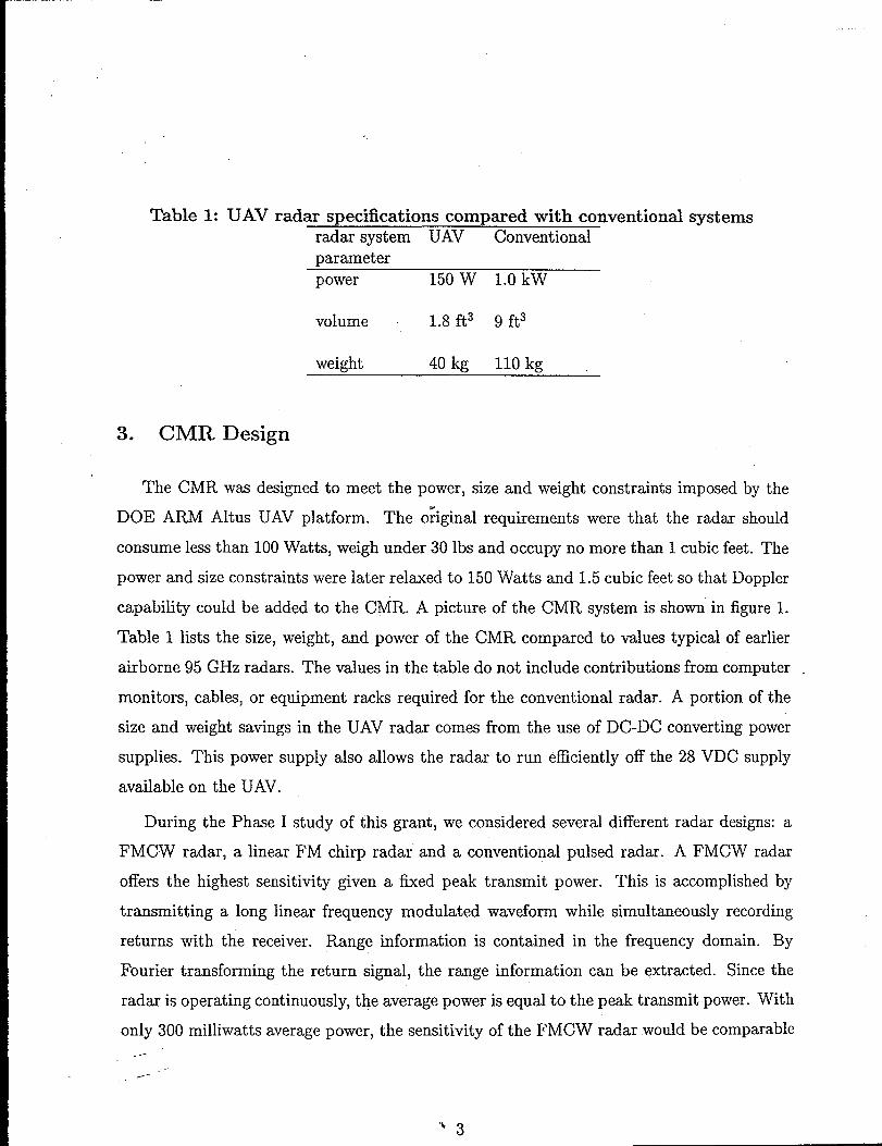
Table 1: UAV radar specifications compared with conventional systemsradarsystem UAV Conventionalparameterpower 150 W 1.0 kW

I volume 1.8 ft3 9 ft3

weight 40 kg 110 kg

3. CMR Design

The CMR was designed to meet the power, size and weight constraints imposed by the

DOE ARM AItus UAV platform. The o&inal requirements were that the radar should

consume less than 100 Watts, weigh under 30 lbs and occupy no more than 1 cubic feet. The

power and size constraints were later relaxed to 150 Watts and 1.5 cubic feet so that Doppler

capability could be added to the CMR. A picture of the CMR system is shown in figure 1.

Table 1 lists the size, weight, and power of the CMR compared to values typical of earlier

airborne 95 GHz radars. The values in the table do not include contributions from computer

monitors, cables, or equipment racks required for the conventional radar. A portion of the

size and weight savings in the UAV radar comes from the use of DC-DC converting power

supplies. This power supply also allows the radar to run efficiently off the 28 VDC supply

available on the UAV.

During the Phase I study of this grant, we considered several different radar designs: a

FMCW radar, a linear FM chirp radar’ and a conventional pulsed radar. A FMCW radar

offers the highest sensitivity given a fixed peak transmit power. This is accomplished by

transmitting a long linear frequency modulated waveform while simultaneously recording

returns with the receiver. Range information is contained in the frequency domain. By

Fourier transforming the return signal, the range information can be extracted. Since the

radar is operating continuously, the average power is equal to the peak transmit power. With

only 300 milliwatts average power, the sensitivity of the FMCW radar would be comparable-------

“b 3

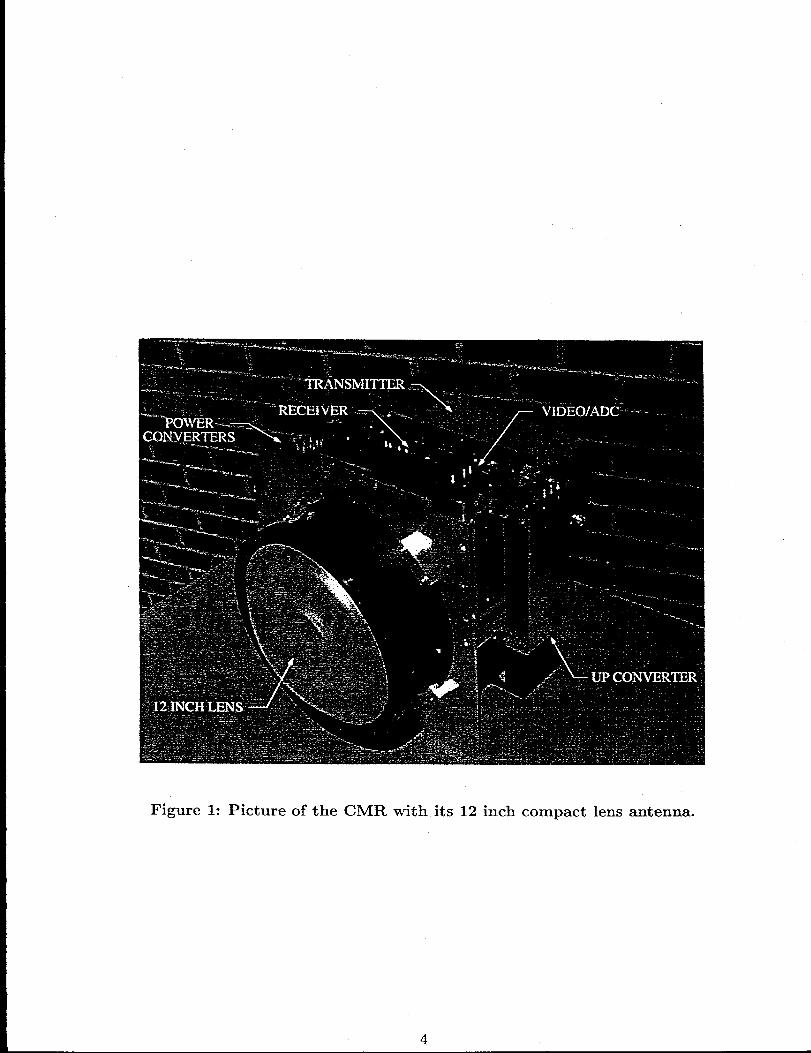
Figure 1: Picture of the CMR with its 12 inch compact lens antenna.

4

to conventional W-band airborne radar systems. Unfortunately, a FMCW system operates

under the assumption that the round trip time to the farthest range extent of interest is an

order of magnitude smaller than the integration time. Since the UAV is expected to operate

at altitudes greater than 15 km (a roundtrip time of 100 usec) and the decorrelation time of

clouds at W-band is less than 500 usec, this requirement could not be satisfied.

A linear FM chirp design also provides another method for obtaining high sensitivity with

low peak power. Like the FMCW system, the transmit waveform is frequency modulated

allowing the pulse length to be extended. The received signal can be compressed by using a

matched filter. The range resolution is related to the bandwidth of the frequency modulation

and not the transmit pulse length. The average power is increased since much longer pulses

can be transmitted compared to that transmitted with a conventional pulsed radar. To

implement a the transmit chirp waveform and matched filter receiver, we consider using a

pair of surface acoustic wave (SAW) devices. However, these devices are difficult to matched,

and result in less than 30 dB range sidelobe performance. This is not be adequate for

clouds applications where the dynamic range can exceed 60 dB at W-band. Higher range

resolution performance on the order of 50 to 60 dB had been demonstrated using a direct

digital synthesizer to generate the chirp waveform and a digital matched filter receiver to

compress the received signal. Unfortunately, the power and size of the data acquisition

system required to do these operations far exceeded our power and size budget. For these

reasons, we determined that a conventional pulsed radar was the only design that could be

used. At that time, Millitech Corporation was developing a 38 Watt peak power W-band

transmitter and a W-band low noise amplifier (LNA) that would allow us to build a compact

W-band radar with reasonable sensitivity, approximately -20 dBZ at 1 kilometer. This was

deemed acceptable, and UMass designed and built this radar.

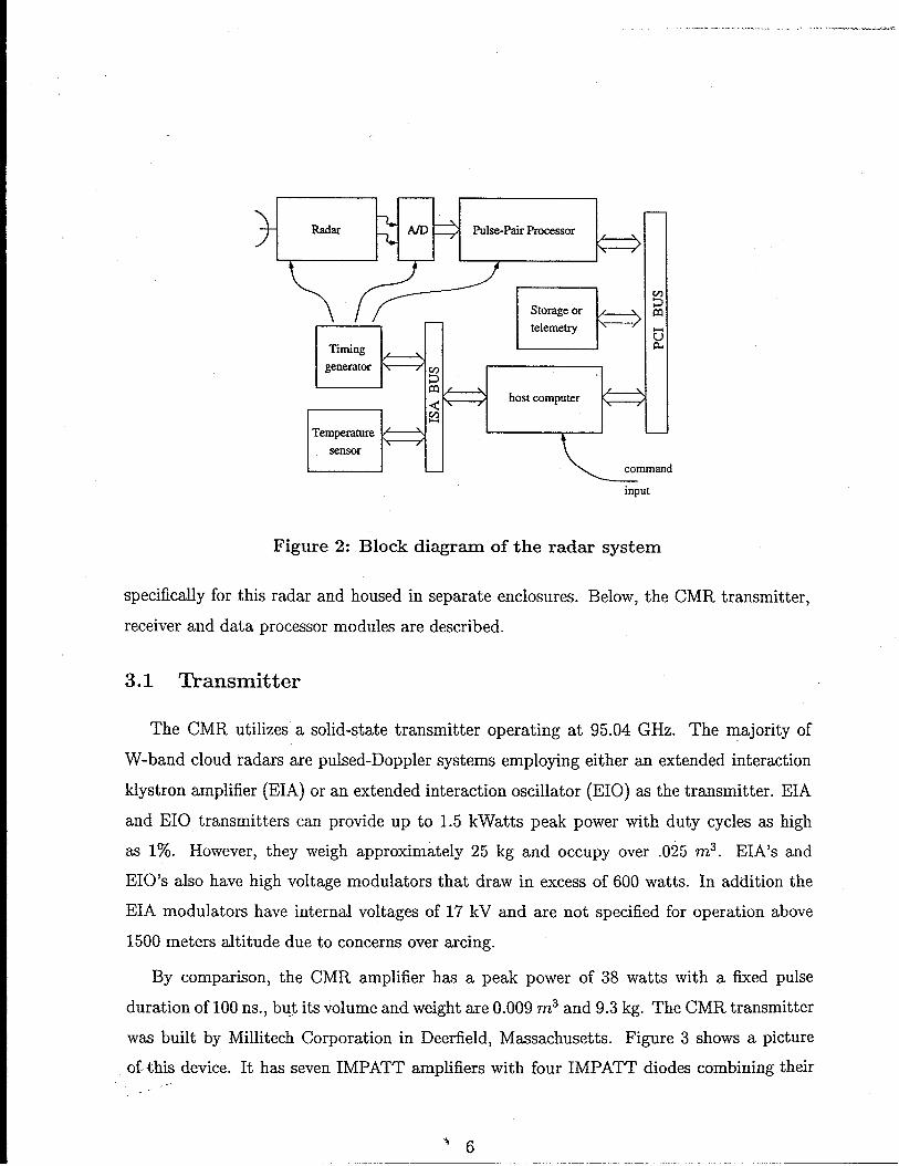
Figure 2 presents the CMR system block diagram, and Table 2 lists the specifications.

Due to the uncertainty in location where CMR would be installed, a modular design was

used to allow for the ,most flexibility in integrating the CMR into the UAV payload. The

transmitter, receiver, power-supply, and analog-to-digital converter (ADC) were all designed

‘5

Radsr-L --+ Pulse-PairProcessorx m -

+ f +

\ /“77p+Timing

generatorg

< \ / host computer~

Temperature

sensorI I u \ commsnd

.... . ..... ..... ...... .. .. ------- .. . .........

input

Figure 2: Block diagram of the radar system

specifically for this radar and housed in separate enclosures. Below, the CMR transmitter,

receiver and data processor modules are described.

3.1 Transmitter

The CMR utilizm’ a solid-state transmitter operating at 95.04 GHz. The majority of

W-band cloud radars are pulsed-Doppler systems employing either an extended interaction

klystron amplifier (EIA) or an extended interaction oscillator (EIO) as the transmitter. EIA

and EIO transmitters can provide up to 1.5 kWatts peak power with duty cycles as high

as lYo. However, they weigh approximately 25 kg and occupy over .025 m3. EIA’s and

EIO’S also have high voltage modulators that draw in excess of 600 watts. In addition the

EIA modulators have internal voltages of 17 kV and are not specified for operation above

1500 meters altitude due to concerns over arcing.

By comparison, the CMR amplifier has a peak power of 38 watts with a fixed pulse

duration of 100 ns., but its volume and weight are 0.009 m3 and 9.3 kg. The CMR transmitter

was built by Millitech Corporation in Deerfield, Massachusetts. Figure 3 shows a picture

of-this device. It has seven IMPATT amplifiers with four IMPATT diodes combining their. -

‘$ 6

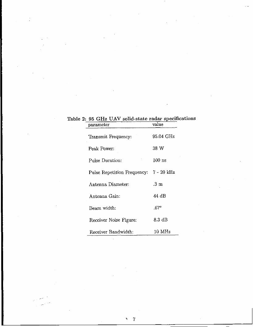
Table 2: 95 GHz UAV solid-state radar specificationsparameter value

Transmit Frequency: 95.04 GHz

Peak Power: 38 W

Pulse Duration: 100 ns

Pulse Repetition Frequency: 7-20 kHz

Antenna Diameter: .3 m

Antenna Gain: 44 dB

Beam width: .67°

Receiver Noise Figure: 8.3 dB

Receiver Bandwidth: 10 MHz

/-

---

“’ 7

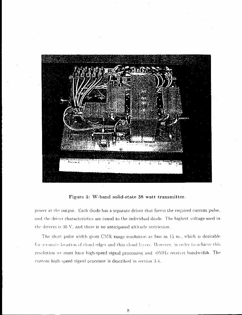
Figure 3: W-band solid-state 38 watt transmitter.

powwr at (he output. Each diode has a separate dri~wr- that. forms the req[lircd current pulse.

and thr dril”cr characteristics are tuned to the indi~idual diode. The highest \oltage used in

thf’ driver~ is :36 I?, and t.h[~reis no anticipated altitud[~ restriction,

Th(: short pulse width gives C\l R range resolution as

ft)r a(fIIr;~[[ Ii)tatif)rl of (1011(1[ldg[+ and thirl (lt)LI(i Iii, i(r>

rw)lution Iv{’must have high-speed signal processing and

custort] higtl-speed signal processor is described in sect ion

3.2 Receiver

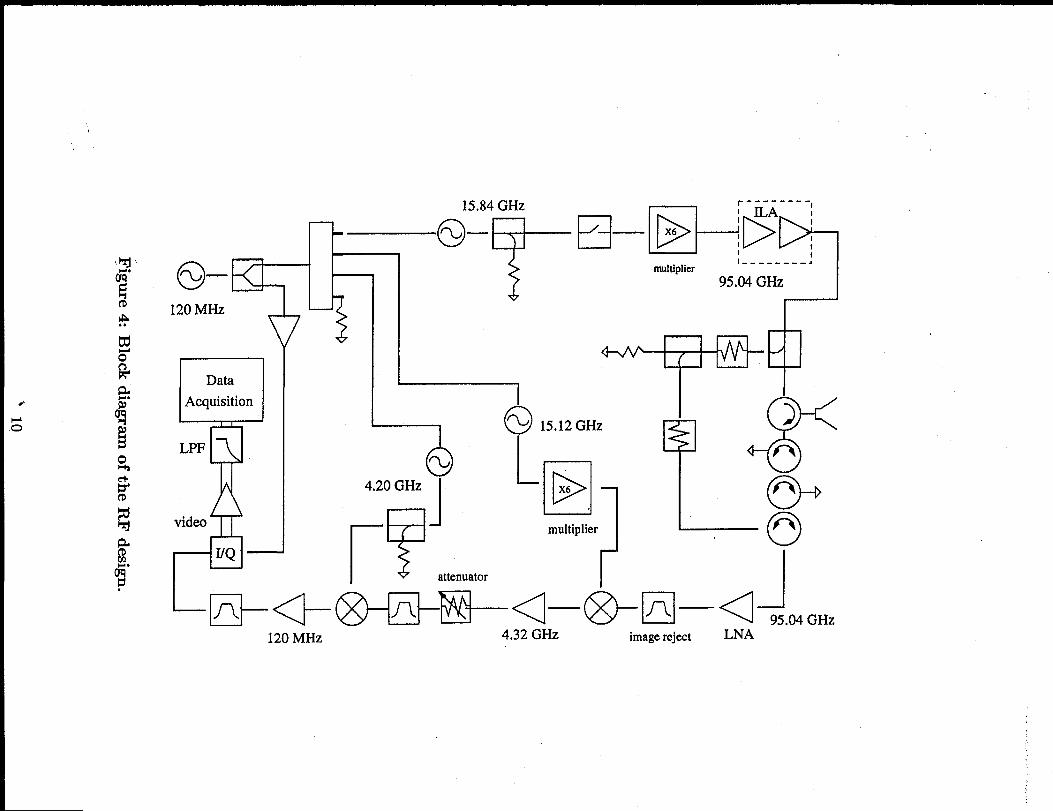
A superheterodyne design is employed in the receiver with intermediate frequencies (IFs)

at 4.32 GHz and 120 MHz. The components of the receiver are included in figure 4. Gain

I is distributed approximately evenly through the receiver chain in a fashion that avoids the

I need for mixers with high LO drives. The W-band LNA has a gain of 22.5 dB at 95.04 GHz

I and a noise figure specification of 7 dB. A high-pass filter follows the LNA to reject noise

at the image frequency of the W-band mixer. The 95.04 GHz RF signal is mixed down to

the 4.32 GHz IF using a double-balanced mixer. The LO for the W-band mixer is generated

I using a 15.12 GHz DRO and a 6x multiplier. A C-band IF was chosen in favor of one

Iat a lower frequency to avoid a sharp cutoff requirement for the W-band image-rejection

filter. This allowed the use of a low insertion-loss filter that would have no measurable

effect on the receiver noise figure. The 4.32 GHz IF amplifier has a gain of 25 dB and

I .1 dB output compression for an input of -16 dBm, which approximately matches the .1 dB

Icompression level of the components that precede it. A demodulator with an LO of 120 MHz

converts CMR’S 120 MHz IF to baseband in-phase (I) and quadrature (Q) components.

The amplification at 120 MHz is set so that the maximum signal levels entering the IQ

I demodulator are within its linear region approximately 10 dB below its ldB compression

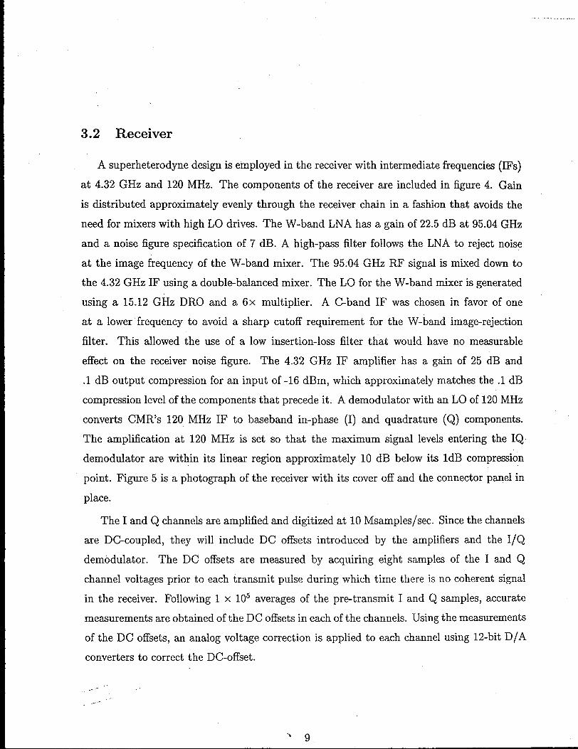
Ipoint. Figure 5 is a photograph of the receiver with its cover off and the connector panel in

place.

The I and Q channels are amplified and digitized at 10 Msamples/sec. Since the channels

I are DC-coupled, they will include DC offsets introduced by the amplifiers and the I/Q

demodulator. The DC offsets are measured by acquiring eight samples of the I and Q

I channel voltages prior to each transmit pulse during which time there is no coherent signal

I in the receiver. Following 1 x 105 averages of the pre-transmit I and Q samples, accurate

measurements are obtained of the DC offsets in each of the channels. Using the measurements

of the DC offsets, an analog voltage correction is applied to each channel using 12-bit D/A

converters to correct the DC-offset.

/-

“’ 9

DataAcquisition

LPF

video

‘ IfQ —

15,84 GI-Iz

@-p=+

120 MHz

El–------ --

pj–l-[pjj-L I I I

I ------- -4multiplier

95.04 GHz

L

O%4,20 GI-Iz

F?.-l

attenuator

U- 15.12GHz

1- ❑X6 -

multiplier

r

7-13Hp

[

44

1 FF+@HEF!i!!l—d-@Fl-Q7L4G.z

120 MHz 4,32 GHz imagereject LNA

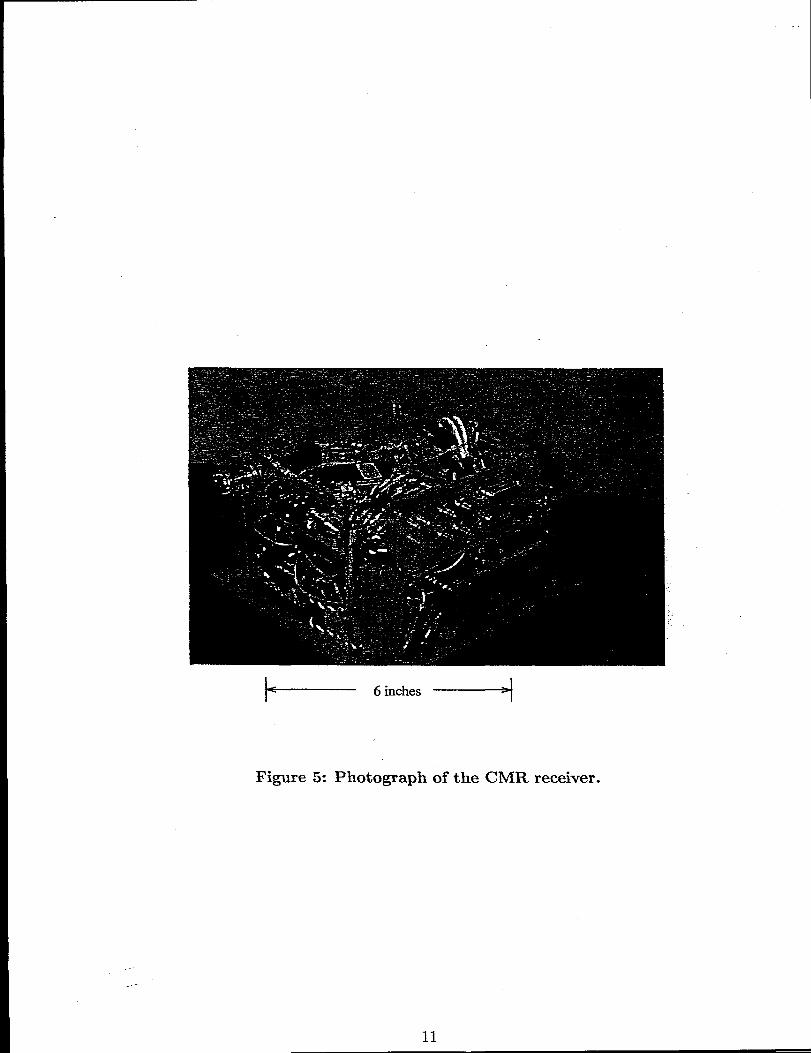
Figure 5: Photograph of the CMR. receiver.

11

3.3 Transmitter-receiver isolation, and internal calibration

The transmitted and received signals are duplexed by a fixed circulator. Approximately

107 dB isolation is provided by the combination of a series of latching circulators and the

fixed circulator. The three latching circulators are contained within a single assembly with

two states, a high isolation state and a low insertion-loss state. During transmit, the latching

circulator assembly is set to a state giving 87 dB isolation, and on receive the insertion loss

is 1.5 dB.

A portion of each transmit pulse is coupled into the receiver through a set of attenuators

and couplers with stable insertion loss. The power in this coupled pulse gives a measure

of the combined gain of the transmitter and receiver. This signal is digitized and used to

remove gain fluctuations during calibration. (Insertion loss through the latching circulators

has been observed to be stable. However, this loss is measured in combination with the

antenna gain during internal calibrations.)

3.4 Data acquisition

The goal for the CMR signal processing system was to achieve the greatest possible

sensitivity improvement available through sample averaging. This is accomplished by trans-

mitting pulses at the maximum repetition rate suitable for the required unambiguous range

and averaging all the profiles within a given period of time. In previous cloud radars it was

necessary to restrict the number of range gates processed or to process only a subset of pulses

that could be transmitted in a given period or to restrict both. Since the potential applica-

tions of CMR include monitoring cloud coverage, it was deemed important to process all the

data within the unambiguous range. The A/D sample rate of the I and Q video channels was

set to 10 MHz to match the available range resolution dictated by the 100 ns pulse width.

Using 12 bit A/D samples, the resulting input data rate is 240 Mbit/second, which is too

high to be stored practically over long periods of time. Computations of reflected power and

autocovariance must be performed in real-time, and the results averaged prior to output to

r~duce the data rate.

---- -

‘$ 12

Omlnnmnan

----- ------ ------ ----[1II1IIIIItIII11t1II11III11I

)/m r %---=------t-i---------l

rlTiming

L,l (tt

Hard lYA converter IGenerator It

Disk ttI1II1Isingle-board

computer F II 1!

‘------------------- computerchassis1---- ---- ----- ---- ---—- ----

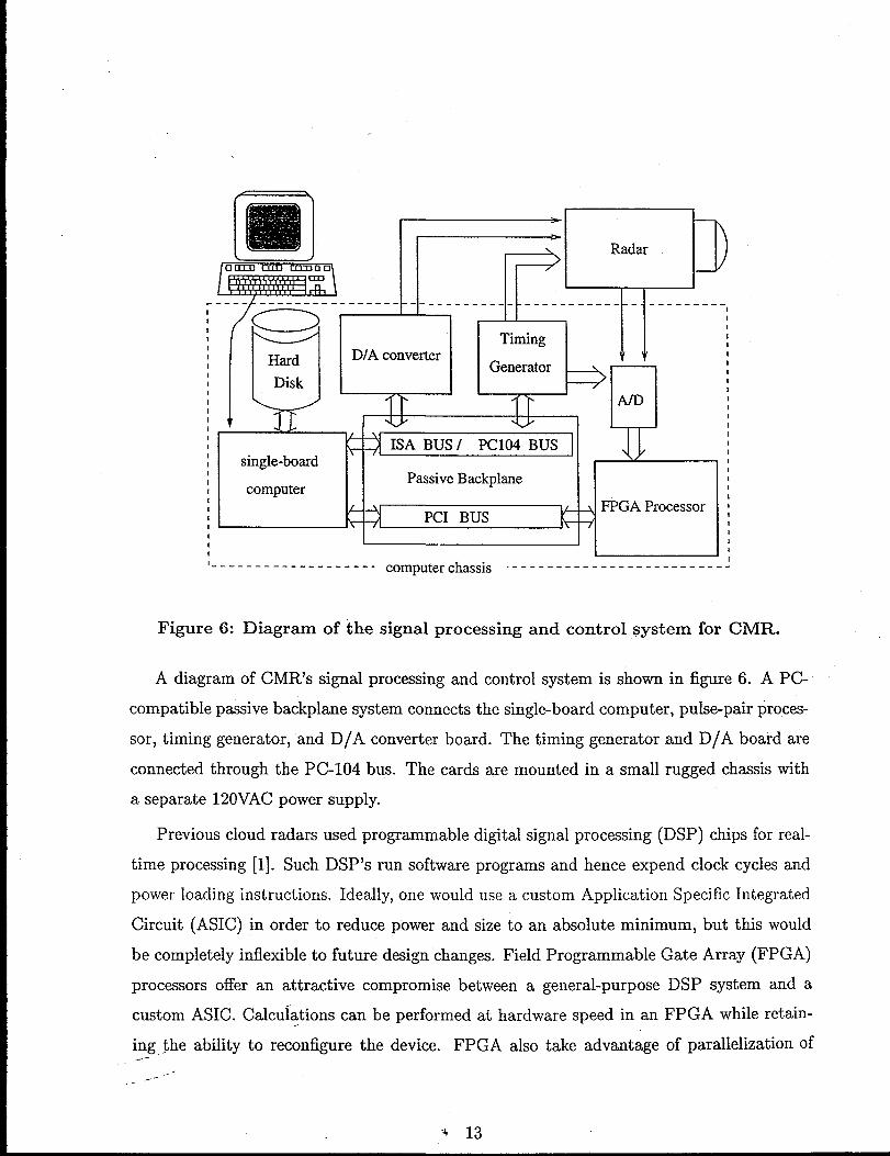
Figure6: Diagram of thesignal processing andcontrol system for CMR.

Adia~am of CMR'ssi~al processing andcontrol system isshowinfi~re6. APC-

compatible passive backplane system connects the single-board computer, pulse-pair proces-

sor, timing generator, “and D/A converter board. The timing generator and D/A board are

connected through the PC-104 bus. The cards are mounted in a small rugged chassis with

a separate 120VAC power supply.

Previous cloud radars used programmable digital signal processing (DSP) chips for real-

time processing [1]. Such DSP’S run software programs and hence expend clock cycles and

power loading instructions. Ideally, one would use a custom Application Specific Integrated

Circuit (ASIC) in order to reduce power and size to an absolute minimum, but this would

be completely inflexible to future design changes. Field Programmable Gate Array (FPGA)

processors offer an attractive compromise between a general-purpose DSP system and a

custom ASIC. Calculations can be performed at hardware speed in an FPGA while retain-

ing the ability to reconfigure the device. FPGA also take advantage of parallelization of---..--

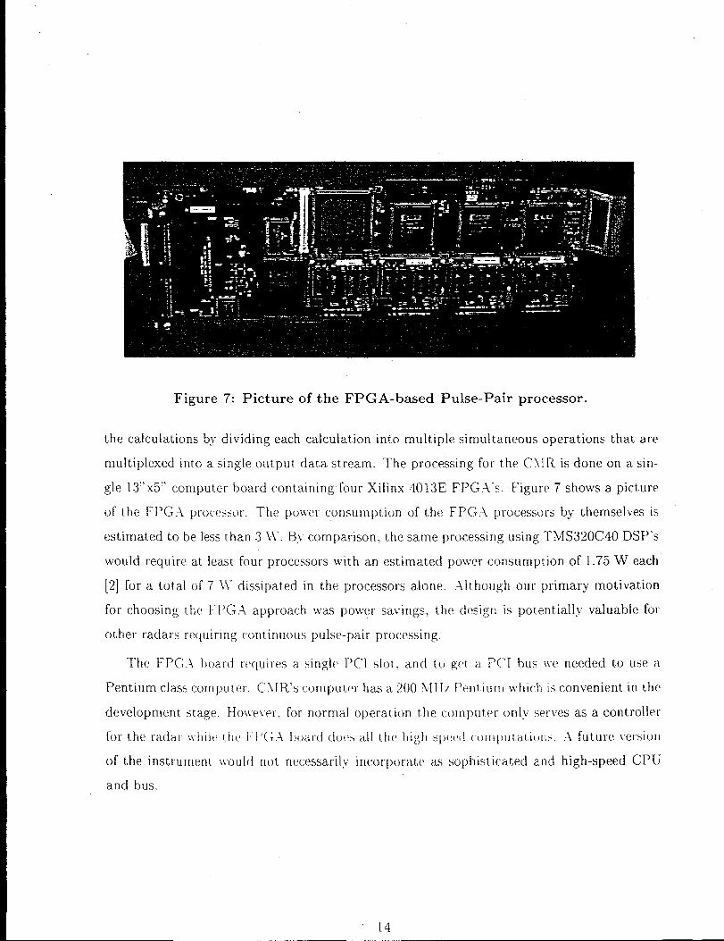
Figure 7: Picture of the FPGA-based Pulse-Pair processor.

the calculations by dividing each calculation into multiple simultaneous operations that are

multiplexed into a single output data stream. The processing for the C\[R is done on a sin-

gle 13’’x5° computer board containing four Xilinx 4013F, FPC,.!”S. Figure 7 shows a picture

of the FPC,.J. proces?or. The po~ier consumption of the FPCT.< processors by themselves is

estimated to be less than 311’. By comparison, the same processing using TMS320C40 DSP’S

would require at least four processors with an estimated po~ver consumption of 1.75 W each

[~] for a total of ~ \\- disslpa~,edin the processors alone. .~ltho[,ghour primary motivation

for choosing the FPG.A approach ~vas power savings, th[’ design is potentially valuable for

other radars req[iiring continuous pulse-pair processing.

The FPG.4 l)uard r~’[{uiresa single PCI S1OI. an(i to g(II a PCI bus LYPneeded t.o use a

Pentium class computer. C\[R’s conlputer has a 200 \lHz Petltiur~l ~vhich is convenient in the

development stage. IIoiveler. for normal operation the cornput~~r only ser~es as a controller

fou the raciar wililt’ LIICFP[; .4 Ijoard cio(> ail t.tl[ Iligtl sfjfL(Il (~)r[}[)~jtt~titj[l>..A future [ersiorl

of t,he instrument iroul~i not necessarily incorporate as sophisticated and high-speed CPU

and bus.

‘ 14

4. CMR Performance

Experiments were performed at the University of Massachusetts, Amherst in fall, 1998

and winter, 1999 to determine the performance of the CMR. During these experiments, the

dual-frequency Cloud Profiling Radar System (CPRS)[3] was operated within 60 meters of

the CMR. CPRS is a truck-mounted instrument built at the University of Massachusetts [4].

It contains two radars, one operatingat9492 GHz and another at 33 GHz., although only the

94.92 GHz radar was available during the experiment. It has participated in numerous field

campaigns, and its performance is recognized as a standard in the meteorological community.

Table 3 gives the CPRS specifications relevant to the comparison. The transmitter used

by CPRS is an extended interaction klystron that provides 1.3 kWatt peak power and pulses

of 500 ns duration. Prior to averaging CPRS has almost 27 d13greater sensitivity than CMR.

Additionally, the radars are mounted on a positioner that facilitates external calibration with

a corner reflector.

The CPRS radar has heaters and temperature control, but lacks an internal calibration,

so changes in the transmitter and receiver gain directly impact the reflectivity values it

measures. This was a particular concern during the winter experiments because CPRS was

stored outdoors, where temperatures were near freezing. Prior to taking data, CPRS was

operated for an hour to allow its temperature to stabilize.

4.1 Experiment - Weather Conditions

The clouds observed on 24 September, 1998 were non-precipitating and multilayered with

a base heights near 4 km. The prevailing winds were approximately along the direction from

CPRS to CMR. Heavy snowfall occurred on the 13th and 14th of January, 1999. Both

radars were covered with nylon tarpaulins, which may have produced some loss, but since

they were made of the same material, we expect that both radars experienced nearly the

same loss. The snow was removed from the antennas frequently to

to accumulation. The snow made the direction of clouds motion

.-

reduce uncertainties due

less obvious than on 24

Table 3: CPRS 94.92 GHz radar specifications.

September, 1998.

radar system CPRS CMRparameter

peak transmitter power 1.3kW 30.5W

noisefigure (dB) 13.0 10.7

receiver bandwidth (MHz) 2 10

1

4.2 Measurements

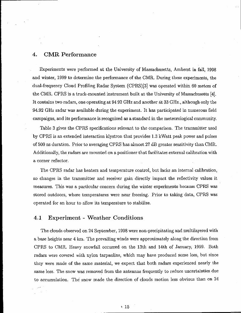
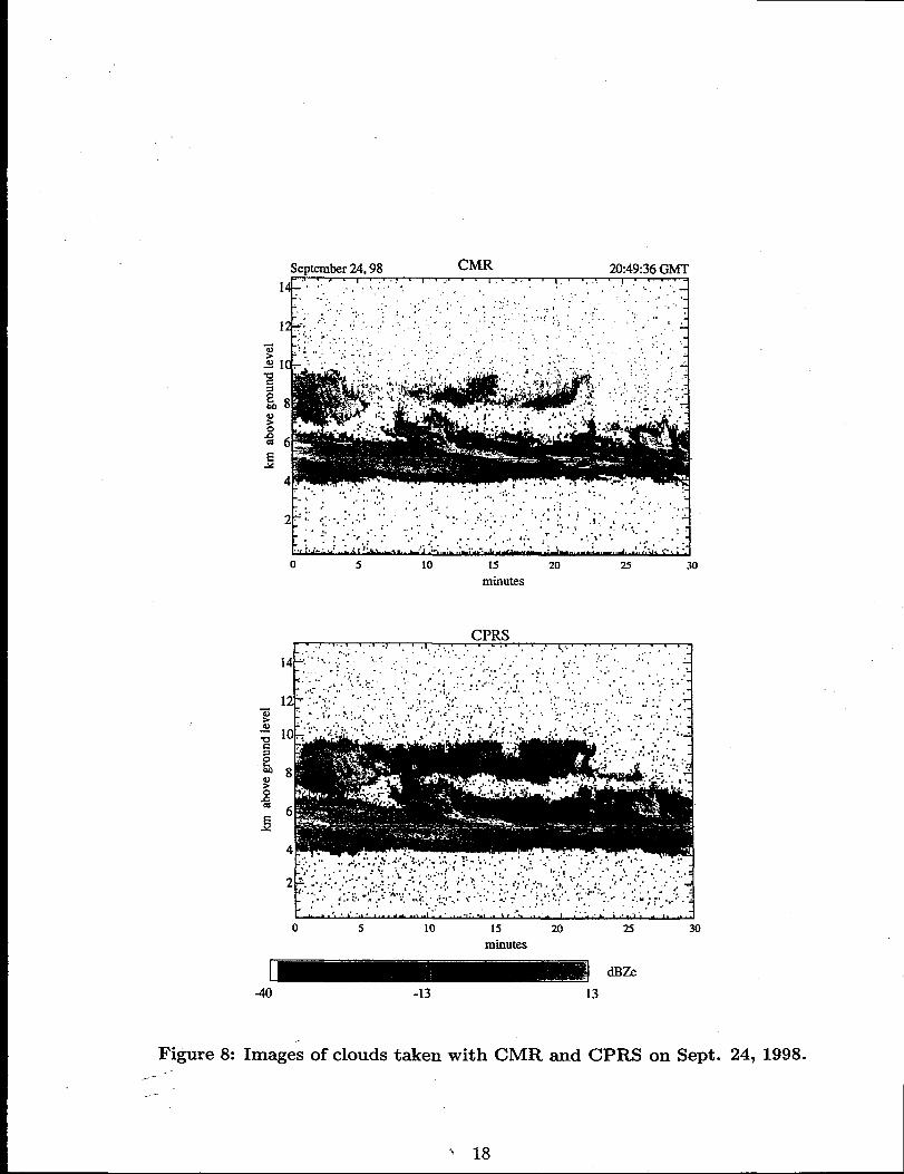
Figure 8 shows images of one minute averaged reflectivity profiles of the clouds measured

by CMR and CPRS on 24 September, 1998. Two layers are visible in both images. Although

the CMR does not demonstrate the same sensitivity as CPRS, it is still able to image both

layers. In this case, the CMR would have been a nice complement to the Cloud Detection

Ladir (CDL). It is likely that much of upper layer would have been opaque to the CDL, and

only a single layer would have been reported when that occurred. From 12 km a down-looking

CMR would have detected both layers at all times, which could have been a valuable detail

given the large height difference and therefore temperature difference between the layers.

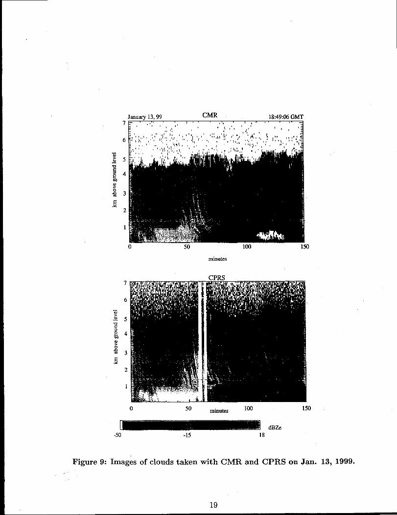
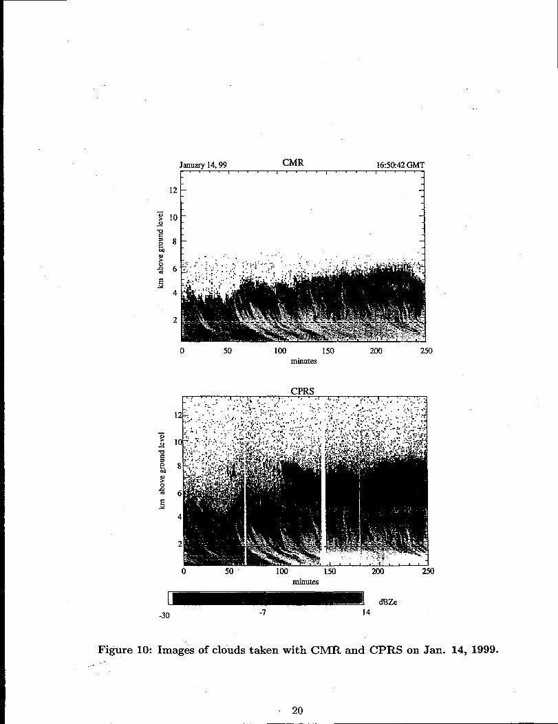
Figure 9 and figure 10 are images of the clouds and precipitation observed during the

winter experiment. The precipitation came in the form of snow consisting of short needles,

graupel and stellar crystals. The data collected on 13 January, 1999 for both radars were

averaged for ten seconds. The plot of CPRS data clearly shows a system artifact at the

cloud top. Rather than displaying a sharp cloud edge as seen in the CMR image, the data

shows a persistent feature. This was caused by the time-domain response of the logarithmic

detector. Specifically; at range-times corresponding to the cloud top the output of the

logarithmic detector still had a significant response to the strongly reflecting cloud beneath.

Thedata displayed for CPRS for14 January, 1999 were averaged for two seconds, so that

this effect would not be as apparent in the image, and the data for CMR were averaged for

ten seconds.

4.3 CMR Sensitivityy

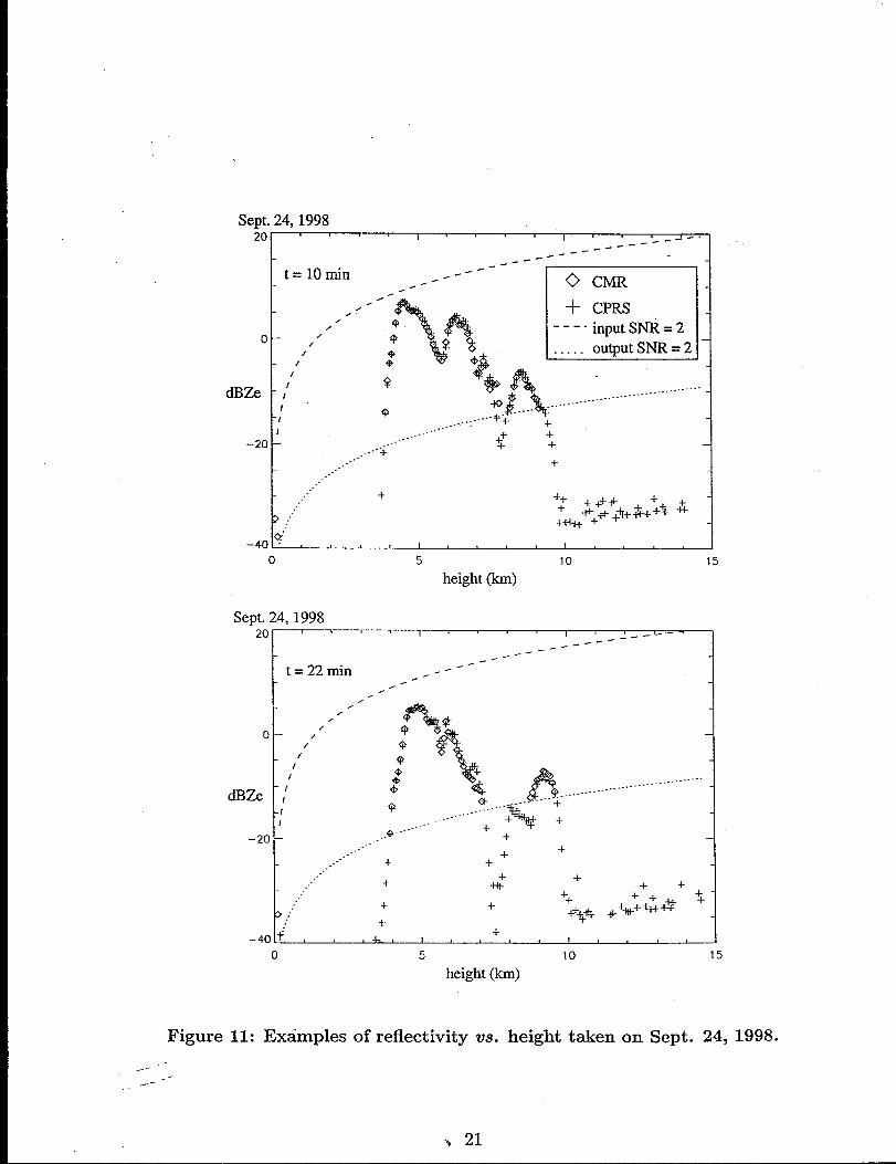
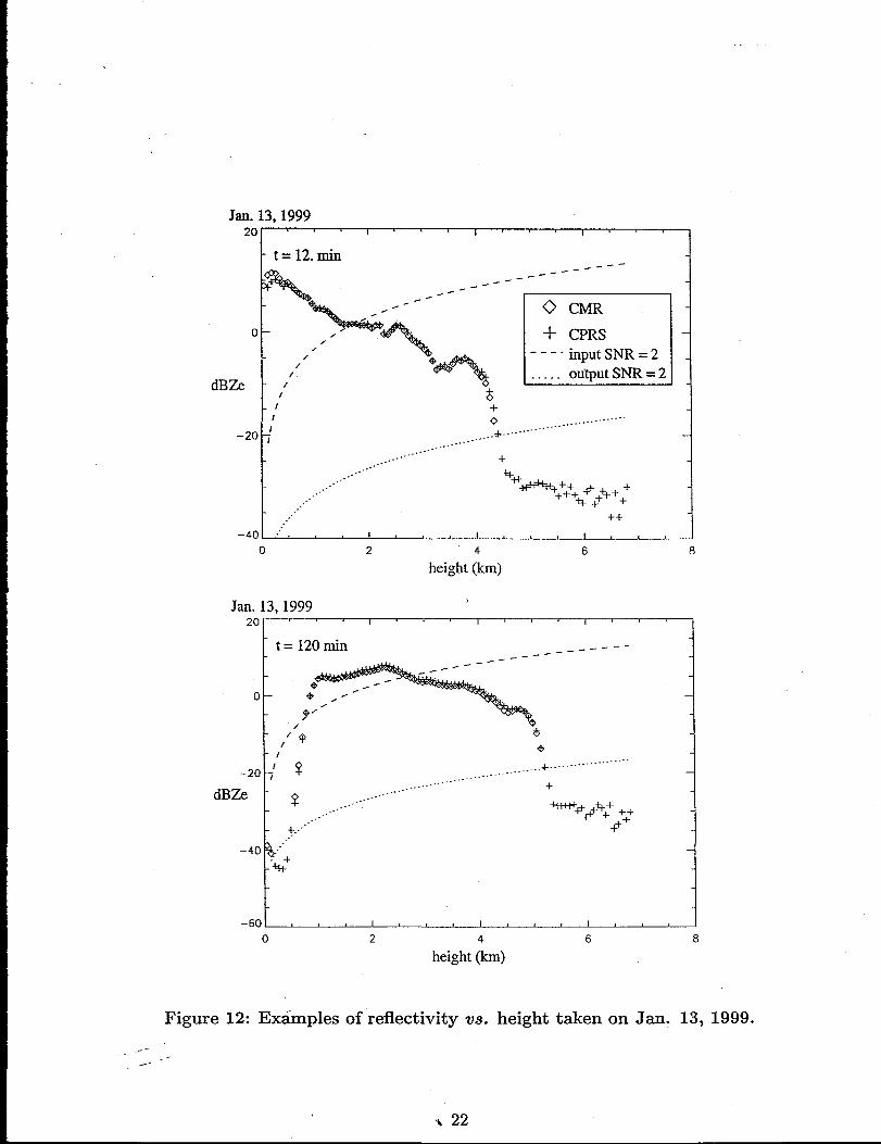
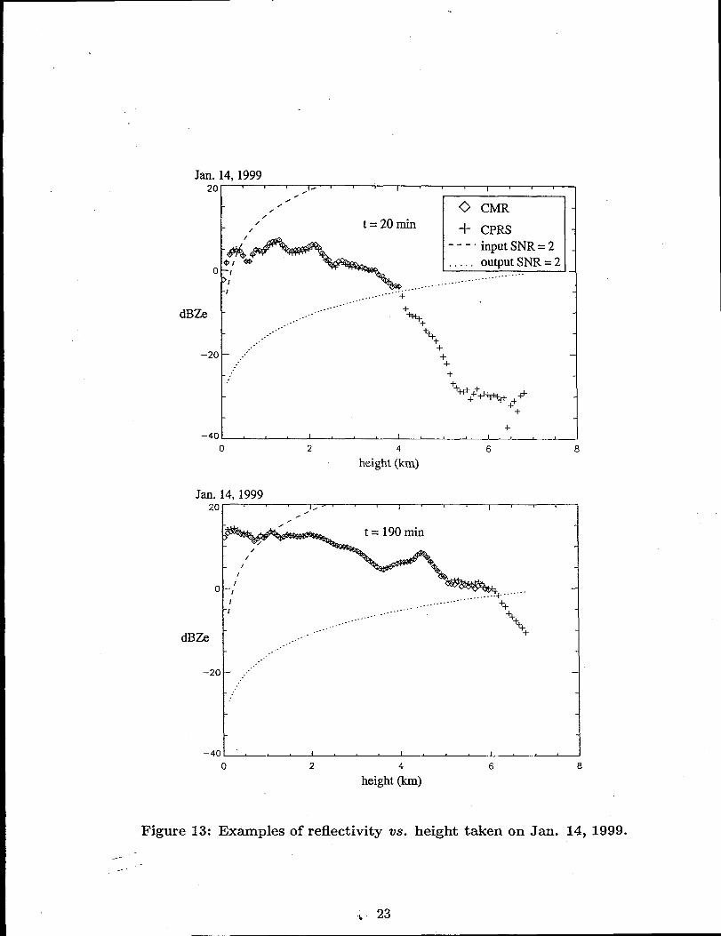
A detection threshold corresponding to a SNR equal two (3 dB) was used when processing

the data in figures 8-10, and this level is plotted as a dotted curve along with the profiles

of reffectivity in figures 11, 12, 13. To illustrate the level of signal processing gain achieved

we have also included a plot of the signal level corresponding to an input SNR of two prior

to averaging, which appears as the upper dashed curve.

An important figure of merit for the performance of a cloud radar is the minimum de.

tectable reflectivity factor, which is directly related to the calibration factor. The minimum

detectable reflectivity factor, dBZ.,~in, is defined as the dBZe value that results in unity

signal-to-noise ratio at a given range [5], which is usually taken to be 1 km. for cloud radars.

With a measurement of the standard deviation of the receiver noise, a., the dBZ.,~in at

1 km is given by

dBZe,~in = lolog~*(cc7n). (1)

The value of a. depends on the receiver noise figure as well as the number of averages

~,~inat 1 km for CMR assuming 5 x 105 averages, and figure 14performed. Table 4 lists dBZ

plots dBZ.,~in as a function of range for the winter instrument configuration. The

ence between measured and predicted dBZ e,minresults directly from the discrepancy

measured and predicted calibration constants.

differ-

in the

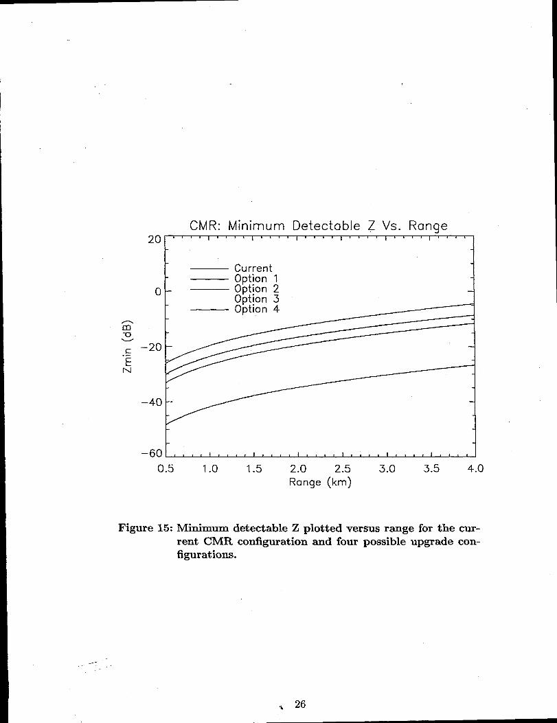
5. CMR Upgrades

Currently CMR has a sensitivity of approximately -20 dBZ at 1 km. This does not meet

the needs of all ARM-UAV science team members. There are a few hardware upgrades that/-

‘+ 17

o 5 10 15 20 2s 30minutes

o 5 10 15 xl 25 30

minutes

40 -13 13

Figure 8: Images of clouds taken With CMR, and CPRS cm Sept. 24, 1998./-

Jsnuary 13,99 CMR 18:49(K GMT,’ ,4;’ ,’ ;, 1’ ,,

1 ,,

! ., ! ,’, ‘ .,’1,

!’,,,,

‘ 1! ,48, ,,,

.,, ,,, ,:,’4 ’1,,, ,’, ,,16

‘4

,,,,,’ 1,’ ,’ “, “’’,4’, : ( ,, “1 1, ,’ , !/, :l:,,; ,,’l ,,, I ~, , :,,\,:: ;;,:,., ’,; ,1, .;, ::::{l

. . . .. . .

5

4

3

2

1

0 50 100 150

minutes

I .50 50 minutes 100

d33ze-50 -15 18

150

Figure 9: Images of clouds taken with CMR and CPRS on Jan. 13, 1999.

19

..

January 14.99 CMR 16:5&42 GMT

o 50 100 150 200 250minutes

CPRS...!. ‘.‘..(ii .;-~~‘.’.!;.’. “r ‘ .: 4.;: .’ “ 6:...-.(. “-, .:.,. ... . . !.Y. .,.,.., . :.....-.- . . . . ...”,. .....

t ! I

o 50 100 150 200 250minutes

Cu3z.e

-30 -7 14

Figure 10: Images of clouds taken with CIVIR and CPRS on Jan. 14, 1999....-

\ 20

Sept.24, 199820

0

CiBze

-20

–40

I I -------- -

-------- 1

t=lo

//

//

/I

I

/

I

I

;~<-- =1Q ‘$3’$$ -9 .,, . . ...$..-%+"""""""-"-""""""""-""--..- 1.----.----- ++ +

....””+”” + +i...... +.. J

..”..... +..

..

o 5 10 15

height (km)

Sept. 24, 199820 “ I I ------------

-------t=22min /-/“

,-.“,/,

0 – /’:*$+

/ $?/ @/ @

+ kdBze / 2 ; p’$ ........-...--”””---”””””-”””-”---”-

-1 9 .....-..+. ...%.--”””””+I +%$ +

-20 –.,-* .....-””

+....”... + +

..- + +..”..- + w+

-t-+ +

.. ‘+ ++ ~ -.. +

9:+ + ++fifi

++*= + *i-

-40 ~ 4+

{ I

0 5 10 15

height(km)

Figure 11: Extiples of reflectivity vs. height taken on Sept. 24, 1998.

/- -._ ---

% 21

Jan.13,199920\ I I ( I

1t= 12.min ---

%

----

0 “\””””---” ------,,// %/ e

dBZe I’I $

t.I +

f o–20~ .....+.-.-

...----

0 cm

+ CPRS

‘--- input SNR=2

. . . . . output SNR = 2

.....-----”...-.-..-”’”’”-”

1/..----..... +...-”...-

..-,... -%1-...- +@++;$+*#+$+++..-” +,...... ++

–401 .: ! I I !o 2 4 6 8

height (km)

Jan. 13, 199920 I I I

t= 120 min ----------------

0 – + ,.’

9’ ‘

,“9 &+

-20 ~’ ‘?...........+-.. ---”” ”””””””-’”

......-.........dBZe

...... +$ /......-”””””

-# +++++# +@+~...””-

–40 ~.”””:+

-%

–60 – I I I

o 2

height &)

Figure 12: Exziinples of reflectivity vs. height

6 8

taken on Jan. 13, 1999.

---/-

% 22

Jan.20

0

.

14,1999

........-........--”. . ..-,.-,

If-y,-/// m]0 cm// t=20min + CPRS

4$4;:---- input SNR = 2

.$, e . . . . . output SNR = 2I .....

......-..””””””--.........’”.....+.

‘%++%+

++++‘+*+++4-W--++$

+ 1+

-40 I I I 10 2 4 6 8

height (km)

Jan. 14, 199920

0

CIBze

–20

– 40

Figure 13:

I.-

1 II,-

/

t= 190rnin

@?@@+~

...

..

..

//

! “v %&

I“1 ‘y+. -..-”f .........- ++.....--..”””...----... ++

...-. +++......”. ..” +

. ...’. . .

I I t I0 2 4 6 8

height (km)

Extiples of reflectivity vs. height taken on Jan. 14, 1999.

.----

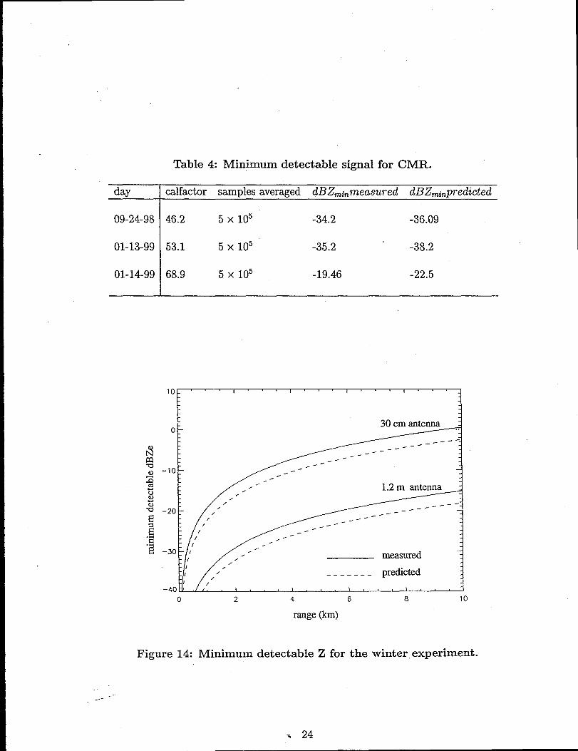
Table4: Minimum detectable signal for CMR.

day calfactor samples averaged dBZ~inmeasured dBZ~inpredkted

09-24-98 46.2 5 x 105 -34.2 -36.09

01-13-99 53.1 5X105” -35.2 “ -38.2

01-14-99 68.9 5 x 105 -19.46 -22.5

30 cm antemao :

-10 :

-----–20 :

–40o 2 4

range(km)

6 8 10

Figure 14: Minimum detectable Z for the winter experiment.

/- -

will dramatically improve CMR’S sensitivity, while still keeping CMR within the size, weight

and power constraints imposed by the Altus platform. The sections below summarize the

upgrades, list their costs and show their impact on CMR’S sensitivity. If all upgrades are

implemented, the CMR sensitivity will improve to -42 dBz at 1 kilometer which meets the

requirements of all science team members.

There are three main modifications to increase CMR’S sensitivity without negatively

impacting the weight, size and power budget for the instrument: reduce transmitter/receiver

bandwidth, install a more efficient compact antenna and improve the receiver noise figure.

These can be broken into four options. Each option is described below. Note that each

option builds off the previous by including all components in the previous option. Figure 15

plots the minimum detectable Z as a function of range for each upgrade option.

5.1 Option 1: Antenna Upgrade

A three-fold compact lens antenna was chosen for the original CMR in order to meet

the volume constraints imposed by the UAV platform. Although small, this type of antenna

has additional loss compared with more conventional lens antennas. Unfortunately, the UAV

platform cannot support a conventional lens antenna due to its large size and shape. However?

W-band cassegrain antennas with integrated radomes can now be purchased. These antennas

will have a gain of 46 dB rather than 44 dB given a twelve inch diameter and occupy slightly

less volume than our compact lens antenna. By using thk antenna, a 4 dB improvement in

the sensitivity will be realized. The cost for the antenna will be no more than $12K. This

includes some NRE costs to customize the antenna for our application.

5.2 Option (2): LNA Upgrade

Recent advancements in W-band low noise

noise figures. CMRS LNA has a noise figure

LNA, a 7 dB improvement will be realized.

/-,..

amplifiers have resulted in LNA’s with 4 dB

of 7 dB. By installing the new antenna and

. 25

su

c.-E

N

20

0

–20

–40

–60

CMR: Minimum Detectable Z Vs. Range-I I I

Current

Option “Odion 2 1Option 3Option 4

I- i I I I I , I ,

0.5 1.0 1.5 2.0 2.5 3.0 3.5 4.0Range (km)

Figure 15: Minimum detectable Z plotted versus range for the cur-rent CMR configuration and four possible upgrade con-figurations.

/-

. 26

5.3 Option (3): Transmitter Upgrade

The solid state transmitter used by CMR can only produce 100 nsec pulses. This results

in a 15-m range resolution which is liner than required. If the resolution could be reduced to

75 m, the required transmitter/receiver bandwidth would be reduce by a factor of 5 and the

volume illuminated would increase by a factor of 5. This would result in a 10 dB improvement

in sensitivity compared to just averaging the five 15-m range cells to get 75 m resolution.

Unfortunately, current W-band technology cannot produce a pulse longer than 100 nsec at

power levels above 1 watt. However, four 300 milliwatt continuous-wave amplifiers can be

power combined to produce a 1 watt W-band amplifier capable of pulse lengths from 100

nsec to continuous-wave (CW). Using this type of amplifier in the CMR transmitter and

a 10 usec linear FM chirp transmit waveform (2 MHz bandwidth), the loss in peak power

can be overcome and a 10 dB improvement in sensitivity realized. Combining this with

the LNA and cassegrain antenna, a total improvement of 17 dB is obtained. Note that

originally we chose not to use a chirp waveform because the data acquisition technology was

not adequate to perform match filtering and Pulse-Pair processing in real-time while staying

within the require power limits. However, recent advancements in FPGA technology will

enable us to perform digital I/Q demodulation, implement a match filter and perform Pulse-

Pair processing with very low power consumption. Furthermore, the 1 watt CW amplifier

will much be more reliable than the 30 Watt 100 nsec transmitter that we currently use in

CMR. In the case that an amplifier fails, the total transmit power will only reduce by 1.3

dB. Replacement diodes only cost $4K and can be installed quickly.

5.4 Option (4): System Upgrade

This is the same as option 3 except that two antennas are used.

ing circulator to the receiver, an antenna can be connected directly

By adding one latch-

to the receiver. Note

that Option (3) suffers from a minimum range/sensitivity tradeoff. As the pulse length is

increase to improve sensitivity, the minimum range is also increased. For a 10 usec chirp,

the closest observable range will be greater than 1.5 km. However, with separate transmit--- -.--

and receive antennas, this problem is overcome because the receiver can be on simultane-

ously with the transmitter. Due to the low transmit powers for CMR, we can obtain enough

isolation between the transmitter and receiver so that we can operate both simultaneously.

This will allow us to transmit much longer pulses, and therefore obtain higher sensitivities

without compromising the minimum range. Furthermore, some of the loss in the receiver

can also be removed. Note that a 40 usec 2 MHz digital matched filter receiver has “already

been implemented on a FPGA processor. In the future, we may be able to extend to even

longer pulses (ie. higher compression gains). It should also be noted that we plan to use a

latching circulator to connect the second antenna directly to the receiver so that CMR can

be electronically switched between a single and a dual antenna mode. This will allow us to

compare both modes in the field and directly measure any errors in the antenna alignments.

The antennas are only 12 inches and we will be integrated into a single structure so that

we don’t expect problems with the alignment. Nevertheless, we will be able to measure

how well the antennas are aligned by comparing the two modes. Mike Ferrario has sent us

ProEngineering drawings of the Altus payload. We have determined that a two antenna

system will not negatively impact any of the other payloads on the aircraft. In fact, the two

antenna system will ultimately require less volume than CMR’S current configuration due

to the large size of the 30 watt solid-state transmitter that will be replaced with the 1 watt

CW transmitter.

[1]

[2]

[3]

REFERENCES

A. L. Pazmany, R. E. McIntosh, R. Kelly, and G. Vali, “An Airborne 95 GHz Dual

Polarization Radar for Cloud Studies”, IEEE Transactions on Geoscience and Remote

Sensing, vol. 1, 1994.

J, Hong, “Calculation of TMS320C40 power dissipation application report”, Tech. Rep.

SPRA032, Texas Instruments, November 1993.

S.M. Sekelsky and R.E. McIntosh, “Cloud observations with a polarimetrc 33 GHz and

95 GHz radar”, Meteorology and Atmospheric Physics, vol. 58, pp. 123-140, 1996.

.+ 28

[4] S. M. Sekelsky, A 33 Gl% and 95

inay estimates of particle size in

Massachusetts, 1995.

GHz Cloud Profiling Radar System (CPRS): Prelim-

and clouds., PhD thesis, University ofprecipitation

[5] R.J. Doviak and D.S. Zrni6, Doppler Radar and

Inc., 1984.

Weather Observations, Academic Press,

...-.