final project report -...

Final Project Report

Mitchell Gu & Ryan BergDecember 9, 2015

6.111 INTRODUCTORY DIGITAL SYSTEMS LABORATORY

MASSACHUSETTS INSTITUTE OF TECHNOLOGY

Contents

1 Introduction 3

2 Technical Overview 42.1 Audio Processing . . . . . . . . . . . . . . . . . . . . . . . . . . . . . 42.2 Game Processing . . . . . . . . . . . . . . . . . . . . . . . . . . . . . 5

3 Audio Processing Implementation - Mitchell 63.1 Overall system organization . . . . . . . . . . . . . . . . . . . . . . . 63.2 Switching from the Labkit to the Nexys 4 . . . . . . . . . . . . . . . 83.3 Sampling the Guitar input . . . . . . . . . . . . . . . . . . . . . . . . 9

3.3.1 XADC input and biasing circuit . . . . . . . . . . . . . . . . . 93.3.2 Oversampling the guitar signal . . . . . . . . . . . . . . . . . 9

3.4 The Fast Fourier Transform . . . . . . . . . . . . . . . . . . . . . . . 113.4.1 Sending samples to the FFT core . . . . . . . . . . . . . . . . 113.4.2 Customizing an FFT block design . . . . . . . . . . . . . . . 133.4.3 XFFT output storage . . . . . . . . . . . . . . . . . . . . . . . 153.4.4 Displaying the spectrum on VGA video output . . . . . . . 15

3.5 Note Recognition . . . . . . . . . . . . . . . . . . . . . . . . . . . . . 163.5.1 Choosing a note recognition strategy . . . . . . . . . . . . . 163.5.2 Saving spectra onto an SD card . . . . . . . . . . . . . . . . . 183.5.3 Developing python scripts to initialize memory with saved

spectra . . . . . . . . . . . . . . . . . . . . . . . . . . . . . . . 193.5.4 The correlator (dot product) modules . . . . . . . . . . . . . 203.5.5 Serializing the divide operation . . . . . . . . . . . . . . . . . 223.5.6 Processing and displaying correlation values . . . . . . . . . 24

3.6 Serializing active notes . . . . . . . . . . . . . . . . . . . . . . . . . . 253.7 Testing the audio processing modules . . . . . . . . . . . . . . . . . 26

1

4 Game Processing Implementation 284.1 Overview of overarching design decisions - Ryan . . . . . . . . . . 284.2 Game control logic - Ryan . . . . . . . . . . . . . . . . . . . . . . . . 30

4.2.1 Song time . . . . . . . . . . . . . . . . . . . . . . . . . . . . . 304.2.2 Simple FSM . . . . . . . . . . . . . . . . . . . . . . . . . . . . 30

4.3 Metadata loading - Ryan . . . . . . . . . . . . . . . . . . . . . . . . . 304.3.1 Overview of Metadata . . . . . . . . . . . . . . . . . . . . . . 304.3.2 Utilization of BRAMs . . . . . . . . . . . . . . . . . . . . . . 31

4.4 Scoring - Ryan . . . . . . . . . . . . . . . . . . . . . . . . . . . . . . . 324.4.1 Parallel matching (37x) . . . . . . . . . . . . . . . . . . . . . . 324.4.2 Parallel metadata request . . . . . . . . . . . . . . . . . . . . 334.4.3 Serializing parallel-matching results . . . . . . . . . . . . . . 334.4.4 Score Tabulation . . . . . . . . . . . . . . . . . . . . . . . . . 344.4.5 Testing scoring . . . . . . . . . . . . . . . . . . . . . . . . . . 34

4.5 Graphics generation - Mitchell . . . . . . . . . . . . . . . . . . . . . 354.5.1 Compressing a high quality background image to fit in BRAM 354.5.2 Generating Note Sprites . . . . . . . . . . . . . . . . . . . . . 37

4.6 Graphics Rendering - Ryan . . . . . . . . . . . . . . . . . . . . . . . 384.6.1 Integrating graphics and the alpha bit approach . . . . . . . 384.6.2 Parallel sprite table access . . . . . . . . . . . . . . . . . . . . 394.6.3 Matching sprites . . . . . . . . . . . . . . . . . . . . . . . . . 40

5 Review and Lessons Learned 415.1 Mitchell . . . . . . . . . . . . . . . . . . . . . . . . . . . . . . . . . . . 415.2 Ryan . . . . . . . . . . . . . . . . . . . . . . . . . . . . . . . . . . . . 42

6 Conclusion 44

References 45

Appendices 46

A Source files 47

2

1. Introduction

The Guitar Hero game genre, pioneered at the MIT Media Lab, consists of a se-ries of games where players play along to rock songs with a custom controllerdesigned to imitate an actual guitar. In the game, players press up to six buttonsthat resemble different frets along with a flip switch that represents the guitarstring at the times indicated on the screen to play the song and earn points. Whilethe game is effective for inspiring many players to learn about guitar, we think itis lacking in realism, song flexibility, and education value. Its six controller but-tons are a far cry from an actual guitar fretboard which has consequences for thegame’s song flexibility. The full spectrum of actual chords in a song become twoarbitrary buttons played at once, and more involved passages must translate intosome combination of the same six buttons. To the user, this is disappointing be-cause they know they are enacting an imitation of how songs are actually played.

Guitar Hero: Fast Fourier Edition is a new take on the genre that enables usersto play with an actual electric guitar as the controller. Furthermore, the song in-structions are displayed on the screen as scrolling tablature, a format universallyavailable and familiar to players when learning guitar songs. The tablature is bothintuitive to read and allows for direct translation of skills learned in-game to thereal world.

Instead of expecting some combination of button presses on a traditional con-troller, the Fast Fourier Edition performs a fast fourier transform of the analogsignal from a guitars pickups to determine what notes are currently active. Fromthe FFT results, the game logic awards the player points depending on their pitchand timing accuracy compared to what was supposed to be played. A graphicaldisplay of the scrolling tablature and supporting graphics will all be output to aVGA monitor. These features will allow users to play their favorite songs andlearn applicable guitar skills along the way.

3

2. Technical Overview

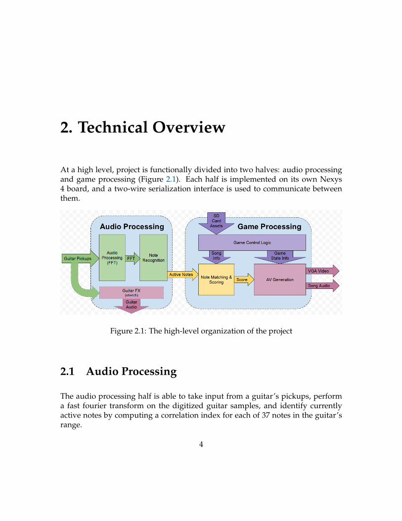
At a high level, project is functionally divided into two halves: audio processingand game processing (Figure 2.1). Each half is implemented on its own Nexys4 board, and a two-wire serialization interface is used to communicate betweenthem.

Figure 2.1: The high-level organization of the project

2.1 Audio Processing

The audio processing half is able to take input from a guitar’s pickups, performa fast fourier transform on the digitized guitar samples, and identify currentlyactive notes by computing a correlation index for each of 37 notes in the guitar’srange.

4

Firstly, the analog signal from a guitar’s pickups is digitized using the Nexys4’s built-in ADC. These digitized samples are then fed through an oversamplingmodule to decrease the sampling frequency before being streamed into a FastFourier Transform module that transforms the signal into the frequency domain.

Once in the frequency domain, it becomes significantly easier to differentiatedifferent notes from each other based on the position of their spectral peaks. Ournote detection method is based on a data-driven, correlational approach that cal-culates correlation indexes between a given frequency spectrum and the referencefrequency spectra of each possible note, played correctly. From these correlationindexes, the system determines which notes are active by first running the indicesthrough a low-pass filter, then imposing adjustable hysteresis thresholds on them.

Once new active notes are calculated, system finally serializes the active notedata and transmits it over two wires to the game processing Nexys to be matchedto actual song notes.

2.2 Game Processing

The game portion takes the active note information from the audio processingportion, and compares it to a song that it knows about to determine how accu-rately a player is playing the song. It displays what the player should be playingon a VGA monitor, and it also displays a score of how well the player has done sofar. It is divided into three major sections, as follows:

The matching and scoring block of the game Nexys receives a serial-encodedlist of the active notes currently being played from the audio Nexys and com-pares them to what notes should be playing currently, as given by the metadata ofthe current song loaded from the SD card. The scoring block scores the player’sperformance appropriately and forwards the score and matched note data to thevideo output.

The AV Generation block takes information about the current score, as wellas the state of the game (playing, paused, song over). It combines graphical as-sets with this information and the song audio to produce a VGA output and anaccompanying audio signal.

The Game control logic block is the backbone of the Nexys 4. It loads assetsfrom an SD card, maintains game state, and handles timing of the scoring module.

5

3. Audio Processing Implementation -

Mitchell

3.1 Overall system organization

Since the project’s initial proposal, there has been a significant overhaul of theaudio processing approach. The most significant of these changes was switchingthe FPGA platform from the 6.111 Labkit that was initially chosen to the Nexys 4.This platform change enabled a lot of improvements to the subsequent modules.The signal chain now includes significant oversampling of the guitar’s input sig-nal, an updated and reconfigured XFFT IP core from Xilinx, and a series of newlydeveloped modules that together facilitate the new data-driven, correlation basednote recognition.

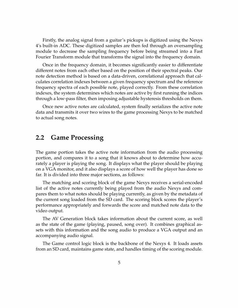
An updated block diagram for the audio processing system is included on thenext page. The sections that follow in this chapter will describe in detail how eachpart of the design was developed and implemented.

6

3.2 Switching from the Labkit to the Nexys 4

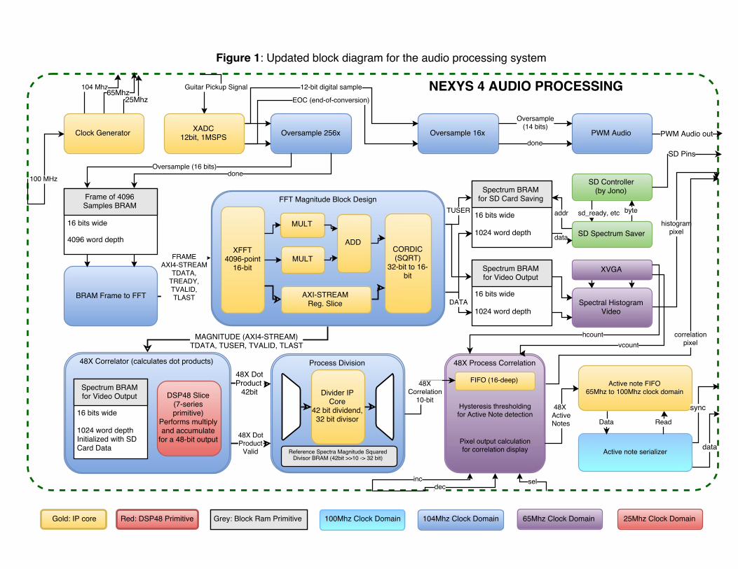
In our initial proposal, we selected the 6.111 Labkit rather than the Nexys 4 boardfor audio processing for several reasons. Firstly, the 6.111 Labkit has an integratedAC’97 audio codec that is well suited to digitizing a guitar pickup signal at 18 bitresolution and a 48khz sample rate. Secondly, we already had experience usingthe AC’97 in Lab 5 of the class, where we recorded, filtered, and down-sampledaudio from a microphone input. Finally, we could base our Fourier Transformimplementation on the provided Fast Fourier Transform demo running on theLabkit.

However, upon starting work with the Labkit, I increasingly found the decade-old development tools cumbersome. For example, the support for Virtex II FPGAused on the Labkit was abandoned in Xilinx’s FFT module generator on ISE (thedevelopment environment) 10.1. In order to reconfigure FFT modules for theLabkit, I needed to create them with ISE 8.1, migrate them over to ISE 10.1, andstruggle to get the module recognized in my existing project. Not only was theprocess inconsistent and time-intensive, but I figured if I was going to learn FPGAdevelopment for future projects, I wanted to learn with the most up-to-date tech-nology and tools.

The more I looked into the newer Vivado development environment and Nexys4 platform, the more I realized that the advantages we had seen in the Labkit hadmore powerful parallels on the newer platform. For audio input, the Nexys 4 hada built-in 12-bit XADC capable of 1 million samples per second. Xilinx’s newerVivado software also offered tight integration of pre-built IP (modules) with theNexys 4 hardware, including the ADC. The Nexys 4’s plentiful digital signal pro-cessing (DSP) slices and faster processing speed gave me more freedom in how Iimplemented the note recognition. Finally, the Vivado software made it easy tostring IP modules together, reconfigure them, and synthesize them out-of-contextto cut down on compile times.

8

3.3 Sampling the Guitar input

3.3.1 XADC input and biasing circuit

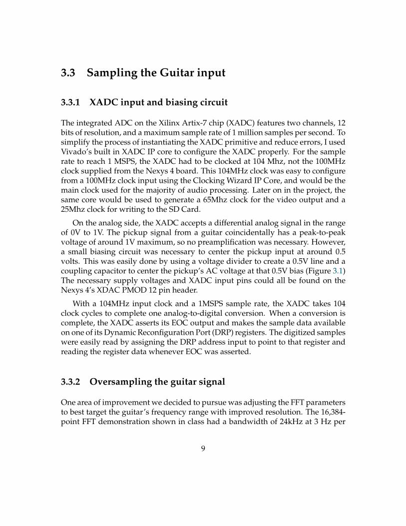
The integrated ADC on the Xilinx Artix-7 chip (XADC) features two channels, 12bits of resolution, and a maximum sample rate of 1 million samples per second. Tosimplify the process of instantiating the XADC primitive and reduce errors, I usedVivado’s built in XADC IP core to configure the XADC properly. For the samplerate to reach 1 MSPS, the XADC had to be clocked at 104 Mhz, not the 100MHzclock supplied from the Nexys 4 board. This 104MHz clock was easy to configurefrom a 100MHz clock input using the Clocking Wizard IP Core, and would be themain clock used for the majority of audio processing. Later on in the project, thesame core would be used to generate a 65Mhz clock for the video output and a25Mhz clock for writing to the SD Card.

On the analog side, the XADC accepts a differential analog signal in the rangeof 0V to 1V. The pickup signal from a guitar coincidentally has a peak-to-peakvoltage of around 1V maximum, so no preamplification was necessary. However,a small biasing circuit was necessary to center the pickup input at around 0.5volts. This was easily done by using a voltage divider to create a 0.5V line and acoupling capacitor to center the pickup’s AC voltage at that 0.5V bias (Figure 3.1)The necessary supply voltages and XADC input pins could all be found on theNexys 4’s XDAC PMOD 12 pin header.

With a 104MHz input clock and a 1MSPS sample rate, the XADC takes 104clock cycles to complete one analog-to-digital conversion. When a conversion iscomplete, the XADC asserts its EOC output and makes the sample data availableon one of its Dynamic Reconfiguration Port (DRP) registers. The digitized sampleswere easily read by assigning the DRP address input to point to that register andreading the register data whenever EOC was asserted.

3.3.2 Oversampling the guitar signal

One area of improvement we decided to pursue was adjusting the FFT parametersto best target the guitar’s frequency range with improved resolution. The 16,384-point FFT demonstration shown in class had a bandwidth of 24kHz at 3 Hz per

9

Figure 3.1: The 0.5V pickup biasing circuit

point, whereas the guitar has a (fundamental) frequency range of 65Hz to 1000Hz.In the lower frequency ranges, a half-step difference in frequency is as little as 5Hz. Thus if we used the FFT as shown in class, only a small range of the outputfrequencies would be useful for identifying notes and the 3Hz resolution wouldbe inadequate for differentiating between low-frequency guitar notes. For thesereasons, I decided to lower the bandwidth of the FFT, which would allow theoutput to fit the guitar’s frequencies better and yield higher frequency resolution.

Due to the principle of Nyquist rates, the sample rate must be decreased inorder to decrease the bandwidth of a Fourier transform. At the XADC sample rateof 1MSPS, the bandwidth of an FFT would be 500 KHz, far higher than necessary.I first considered lowering the bandwidth by simply low-pass filtering and thendownsampling the XADC samples by a certain ratio, as done in Lab 5A of thecourse. However, I felt unsatisfied with discarding the majority of the samplesand instead looked into oversampling the XADC samples.

In oversampling, the signal is sampled at several times the desired samplerate and averaged across the extra samples to arrive at the oversampled sample.Because of the extra information that contributes to sample, the resolution andsignal to noise ratio of the signal can be improved at the expense of sample rate.

I decided to oversample the 1MSPS XADC input at a 256x rate, which increasesthe SNR by

√256 = 16. Consequently, the samples gain log2 16 = 4 extra bits

of precision (16 bits total) and the sample rate decreases to around 4KHz. Atthis sample rate, the FFT bandwidth becomes 2KHz, of which I would use the

10

lower half (0-1KHz) for note recognition. I also settled on an FFT size of 4096points in order for the output of the FFT to have a 1Hz per bucket resolution,three times greater than that of the demo. This higher resolution would be usefulin differentiating low-frequency notes played later on.

Functionally, the oversampling module takes a 12-bits of sample data and theEOC output of the XADC and outputs a 16-bit bus of oversampled data and adone line, which it asserts once every 256 XADC conversions, or once every 256×104 = 26624 clock cycles.

3.4 The Fast Fourier Transform

3.4.1 Sending samples to the FFT core

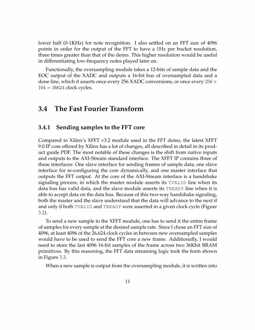
Compared to Xilinx’s XFFT v3.2 module used in the FFT demo, the latest XFFT9.0 IP core offered by Xilinx has a lot of changes, all described in detail in its prod-uct guide PDF. The most notable of these changes is the shift from native inputsand outputs to the AXI-Stream standard interface. The XFFT IP contains three ofthese interfaces: One slave interface for sending frames of sample data, one slaveinterface for re-configuring the core dynamically, and one master interface thatoutputs the FFT output. At the core of the AXI-Stream interface is a handshakesignaling process, in which the master module asserts its TVALID line when itsdata bus has valid data, and the slave module asserts its TREADY line when it isable to accept data on the data bus. Because of this two-way handshake signaling,both the master and the slave understand that the data will advance to the next ifand only if both TVALID and TREADY were asserted in a given clock cycle (Figure3.2).

To send a new sample to the XFFT module, one has to send it the entire frameof samples for every sample at the desired sample rate. Since I chose an FFT size of4096, at least 4096 of the 26,624 clock cycles in between new oversampled sampleswould have to be used to send the FFT core a new frame. Additionally, I wouldneed to store the last 4096 16-bit samples of the frame across two 36Kbit BRAMprimitives. By this reasoning, the FFT data streaming logic took the form shownin Figure 3.3.

When a new sample is output from the oversampling module, it is written into

11

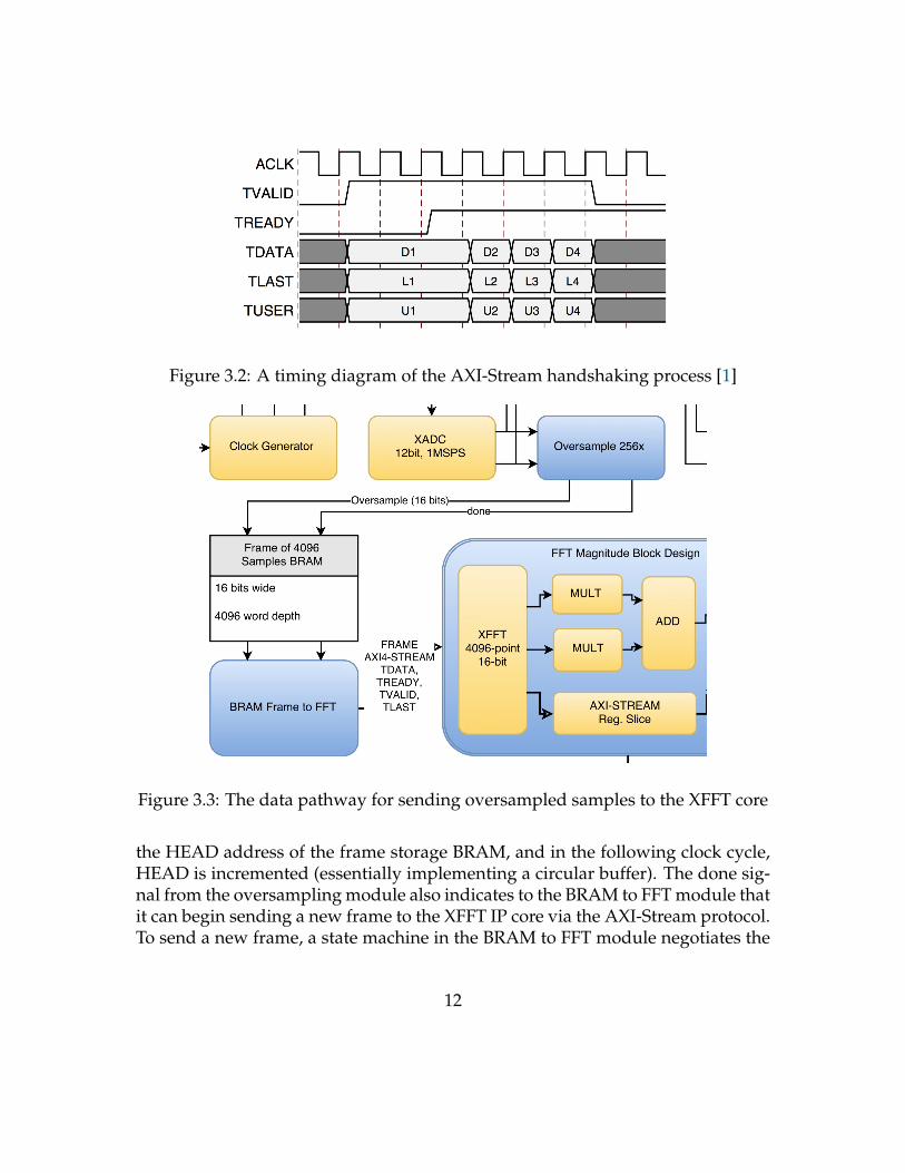
Figure 3.2: A timing diagram of the AXI-Stream handshaking process [1]

Figure 3.3: The data pathway for sending oversampled samples to the XFFT core

the HEAD address of the frame storage BRAM, and in the following clock cycle,HEAD is incremented (essentially implementing a circular buffer). The done sig-nal from the oversampling module also indicates to the BRAM to FFT module thatit can begin sending a new frame to the XFFT IP core via the AXI-Stream protocol.To send a new frame, a state machine in the BRAM to FFT module negotiates the

12

AXI-Stream protocol by outputting sample data from the frame BRAM (startingat HEAD) and incrementing the address to that BRAM whenever the handshakesignaling has succeeded (typically every clock cycle). After 4095 successful datatransfers, it also asserts the TLAST wire to indicate that the last sample in theframe is being sent. If the XFFT core ever thinks the TLAST wire wasn’t assertedon time (there is a misalignment in frame positions), it asserts a last missing wirewhich the BRAM to FFT module uses to realign its frame with the XFFT core.

3.4.2 Customizing an FFT block design

The output (and input) of the XFFT core has both real and imaginary components.In sending samples to the core, only the real component is used, but the output ofthe core will have both real and imaginary components. For the purposes of noterecognition, it is desirable to work with just the magnitude of the FFT output,so a method was needed to convert from real and imaginary components to amagnitude, given by:√

real component2 + imaginary component2

My initial instinct was to compute the magnitude was to write all the necessaryverilog modules, but this would have proved difficult because the square rootmodule would need to be fully pipelined to be able to handle the fully pipelinedoutput from the XFFT core.

Instead, I discovered how to use Vivado’s block design functionality and learnedto appreciate the beauty of the AXI-Stream interface standard. In Vivado’s BlockDesign tool, users can use a graphical interface to connect both Xilinx-providedand user-created IP cores into one abstracted block design that can then be instan-tiated like any other IP core or module (Figure 3.4).

In my FFT Magnitude block design, I was able to connect an XFFT IP core’sAXI output to a pair of multipliers that took both the real and imaginary partsand squared them in parallel. The outputs of these multipliers were then addedand then fed into Xilinx’s CORDIC IP core, which among many functions canperform a square root operation that is fully pipelined. The beauty of the AXIstandard is that the XFFT and CORDIC IP’s both accepted AXI-Stream interfaces,meaning they could be linked in series without the need of any supporting logic.Since I configured the squaring multipliers to have a 1 clock cycle latency, it was

13

Figure 3.4: Vivado’s block design interface

necessary to place a pipeline stage on the AXI interface between the XFFT and theCORDIC. However, this was as simple as inserting an AXI-Stream register sliceIP in between the modules, which handles all handshake signaling as necessary.In this way, I was able to make a simplified FFT magnitude block design that hadexactly the inputs and outputs I wanted without worrying about the implemen-tation details contained within (Figure 3.5).

Figure 3.5: A schematic representation of the FFT Magnitude block design

14

3.4.3 XFFT output storage

In a similar fashion to how samples are stored in a frame BRAM to be sent tothe FFT block, the FFT frequency spectrum output is stored in a spectrum BRAMfor reading as a histogram on a VGA monitor or saving into an SD card. Conve-niently, the AXI-STREAM output of the FFT block includes a TUSER bus in addi-tion to the TDATA bus, which stores the frequency index that corresponds to thecurrent data in the TDATA bus. This TUSER bus was easy to adapt into an addressfor separate BRAMS that store the spectral data for the histogram video outputand SD card saving modules. The XFFT module prefers to give its output mag-nitudes in ”reverse bit order,” which increments its indices starting at the mostsignificant bits rather than the least significant bits. However, using the TUSERindex as an address into a BRAM guarantees that the data will make it into theright slot regardless of order.

For note recognition, I was only interested in the lower 1024 frequency binscorresponding to frequencies less than 1kHz and TUSER values less than 1024(out of a maximum of 4096). Therefore, the write enable port of each BRAM wasonly asserted when both the TVALID AXI line was high and the TUSER value wasless than 1024.

I used one BRAM for histogram video generation and one BRAM for SD Cardbecause both the video module and the SD card saving module run in differentclock domains (65Mhz and 25Mhz respectively). Because the two-port BRAMprimitives allow separate clock domains on each port, they also allow data trans-fer between two clock domains without incurring timing violations. In order toensure stability in multiple clock domain situations, the BRAMS were configuredin ”Write First” mode, per Xilinx recommendation. That way, when a collisiondoes occur and a word is being read and written at the same time, the write willhappen first in order to prevent data uncertainty.

3.4.4 Displaying the spectrum on VGA video output

Once the FFT data was stored in a BRAM, the histogram video module uses theread port of the BRAM to output pixel values that display a spectral histogram. Atany particular horizontal position (hcount), the spectral histogram module onlyoutputs a white pixel if the current vertical position is less than the BRAM datavalue at the address of the horizontal position. This works out to one column of

15

pixels per address (1Hz bucket) across the target resolution of 1024x768 pixels. Inorder for the 16-bit (0 to 65k) FFT magnitude values to fit on the vertical spaceof the monitor, the magnitude was right shifted 7 bits so that the maximum his-togram height possible was 512 pixels. An example histogram output for whenthe guitar’s high E string (≈330Hz) was played is shown in Figure 3.6.

Figure 3.6: An example spectral histogram when a guitar’s high E string is played

Upon first seeing what the spectra looked like, I was pleasantly surprised, asI expected them to be significantly more noisy. Compared to the input from acommon electret microphone, the peaks in the pickup spectra were very clear andstable. The biggest anomaly in the spectrum was the consistent peak at 60Hz,which I assume was caused by mains hum, but since all the guitar frequencieswere above 72 Hz, I figured I could easily crop out everything below 72 Hz.

3.5 Note Recognition

3.5.1 Choosing a note recognition strategy

With the spectra successfully processed and displayed, I needed to settle on amethod for note recognition. The most straightforward approach that I consideredfirst was to implement a peak finding algorithm to detect the frequencies at whichpeaks in the spectrum were centered. However, I felt that this approach would bevery susceptible to anomalies such as harmonics or spurious peaks that were stillpresent in the spectrum. In addition, such an algorithm would likely be expensive

16

with respect to clock cycles because one would have to traverse the spectrum inorder.

Another approach I considered was looking only at the frequency bins at whicheach of the 37 notes under consideration were centered, and evaluate whetherthere presently is a peak there. I felt this was a slightly better method, but stillwould be very susceptible to harmonics and hard to calibrate.

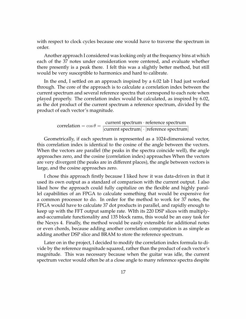
In the end, I settled on an approach inspired by a 6.02 lab I had just workedthrough. The core of the approach is to calculate a correlation index between thecurrent spectrum and several reference spectra that correspond to each note whenplayed properly. The correlation index would be calculated, as inspired by 6.02,as the dot product of the current spectrum a reference spectrum, divided by theproduct of each vector’s magnitude.

correlation = cos θ =current spectrum · reference spectrum|current spectrum| · |reference spectrum|

Geometrically, if each spectrum is represented as a 1024-dimensional vector,this correlation index is identical to the cosine of the angle between the vectors.When the vectors are parallel (the peaks in the spectra coincide well), the angleapproaches zero, and the cosine (correlation index) approaches When the vectorsare very divergent (the peaks are in different places), the angle between vectors islarge, and the cosine approaches zero.

I chose this approach firstly because I liked how it was data-driven in that itused its own output as a standard of comparison with the current output. I alsoliked how the approach could fully capitalize on the flexible and highly paral-lel capabilities of an FPGA to calculate something that would be expensive fora common processor to do. In order for the method to work for 37 notes, theFPGA would have to calculate 37 dot products in parallel, and rapidly enough tokeep up with the FFT output sample rate. WIth its 220 DSP slices with multiply-and-accumulate functionality and 135 block rams, this would be an easy task forthe Nexys 4. Finally, the method would be easily extensible for additional notesor even chords, because adding another correlation computation is as simple asadding another DSP slice and BRAM to store the reference spectrum.

Later on in the project, I decided to modify the correlation index formula to di-vide by the reference magnitude squared, rather than the product of each vector’smagnitude. This was necessary because when the guitar was idle, the currentspectrum vector would often be at a close angle to many reference spectra despite

17

being orders of magnitude smaller in size because nothing was being played. Bydividing by the square of the reference magnitude instead, the new correlationindex effectively scales the cosine of the angle by the ratio between the currentmagnitude and the reference magnitude, which necessitates that the current spec-trum be roughly as ”loud” as it is when a note is actually played.

new correlation =current spectrum · reference spectrum|current spectrum| · |reference spectrum|

· |current spectrum||reference spectrum|

=current spectrum · reference spectrum

|reference spectrum|2

To obtain the reference spectra, I chose the approach of playing each possiblenote correctly four times and saving their spectra to an SD card. Then the spec-tra would be averaged across all four trials to arrive at a reference spectrum thatserves as initialization data for a BRAM on the FPGA chip. Then, as the FFT mag-nitude block design streams its magnitudes and indices to a correlator module,the module could look up the corresponding magnitudes at the same addresseseach reference spectrum BRAM and perform the dot-product in real-time. Thedot product computation would be completed only a few clock cycles after theFFT had finished streaming its frame of magnitudes.

3.5.2 Saving spectra onto an SD card

The first task to tackle was saving the current spectrum to sectors on an SD card.Thankfully, the SD card controller provided by Jono, a previous student, was a bigtime-saver. After importing his controller module, all I needed to do was send theappropriate bytes and control signals to the SD controller.

The SD card must be written in 512 byte sectors at a time. The saved spectraare 1024 words of 16 bits (2 bytes), or 2048 bytes total. Thus each saved spectrummust occupy four sectors on the SD card. The saver module handles this by ad-vancing through one quarter of the spectrum BRAM for SD card data at a timeand signaling to the SD controller module to switch to the next sector before ad-vancing again. While the saver module is saving the BRAM data, it also outputsan active bit that forces the write enable line to the spectral BRAM low to ensurethat no write/read collisions happen while it is saving.

18

Other inputs to the SD card saving module include a start input that is con-nected to the debounced center button, a memory slot selection bus where a usercan select up to 64 different memory slots to record into, and a reset input resetsthe SD controller module and the saver’s internal states. This reset line is oftenuseful for resetting the controller when the SD card wasn’t inserted initially.

3.5.3 Developing python scripts to initialize memory with saved

spectra

Due to the difficulty of implementing filesystem navigation on an FPGA, the SDcard is written in raw binary format as if it were a regular SDRAM. To read thedata on a normal computer, I initially used tools such as wxHexEditor or HexFiend to copy and paste each set of four sectors for processing. However, with40 notes and 8 chords that I wanted to record at 4 trials each, I wanted a quicker,more automated method for parsing the data. I eventually wrote a python scriptthat opened the SD card volume, read the sectors in sets of four as requested bythe user, averaged them, plotted a spectral histogram to confirm that the datawas correct, and translated the data into a .MIF file that could be used to initial-ize a BRAM. The original plan for initializing BRAMS with the reference spectrawas to generate .coe (Xilinx coefficent format) files, which are accepted by theBlock Memory Generator IP for initializing. However, with 48 different .coe files,I would have to generate 48 different IP cores, one for each note. To keep theHDL sources modular and neat, I ideally wanted a solution whereby one corre-lator module could be used for all 48 notes, but parametrized to read from dif-ferent memory files. With a bit of online research, I discovered a different syn-tax for memory initialization that used inferred BRAMs and a function called$readmemb(<file>):

parameter REF_MIF = "../mif/00.mif";

// Inferred bram

reg [15:0] ref_mag [0:1023];

initial $readmemb(REF_MIF, ref_mag);

Because of the register array’s size and the fact that it is read synchronouslyacross a clock edge, Vivado will always infer that ref mag should be implementedas a 16-bit wide by 1024 word deep BRAM. The addition of the readmemb com-mand initializes the BRAM with the contents (in binary) of the REF MIF file, with

19

one word per line. Because REF MIF is a parameter, it can be configured inde-pendently for each instance upon instantiation. The syntax can be paired with agenerator loop in the following concise syntax:

defparam correlator_gen[0].c.REF_MIF = "../mif/00.mif";



// etc...

wire [41:0] dot_product [0:47];

wire [47:0] dot_product_valid;

wire [81:0] debug [0:47];

genvar a;

generate for(a=0; a<48; a=a+1)

begin : correlator_gen

correlator c (

.clk(clk_104mhz),

.magnitude_tdata(magnitude_tdata[15:0]),

.magnitude_tlast(magnitude_tlast),

.magnitude_tvalid(magnitude_tvalid),

.magnitude_tuser(magnitude_tuser),

.dot_product(dot_product[a]),

.dot_product_valid(dot_product_valid[a]),

.debug(debug[a])

);

end

endgenerate

The use of input and output wires in a size 48 unpacked array dimensionmakes indexing into a certain instance’s input and output packed buses easy.

3.5.4 The correlator (dot product) modules

The purpose of each of the 48 correlator modules (see Figure 3.7) is to compute thedot product between the current streaming FFT output and the reference spectrumit has been instantiated with. To achieve this, each correlator module has a BRAM

20

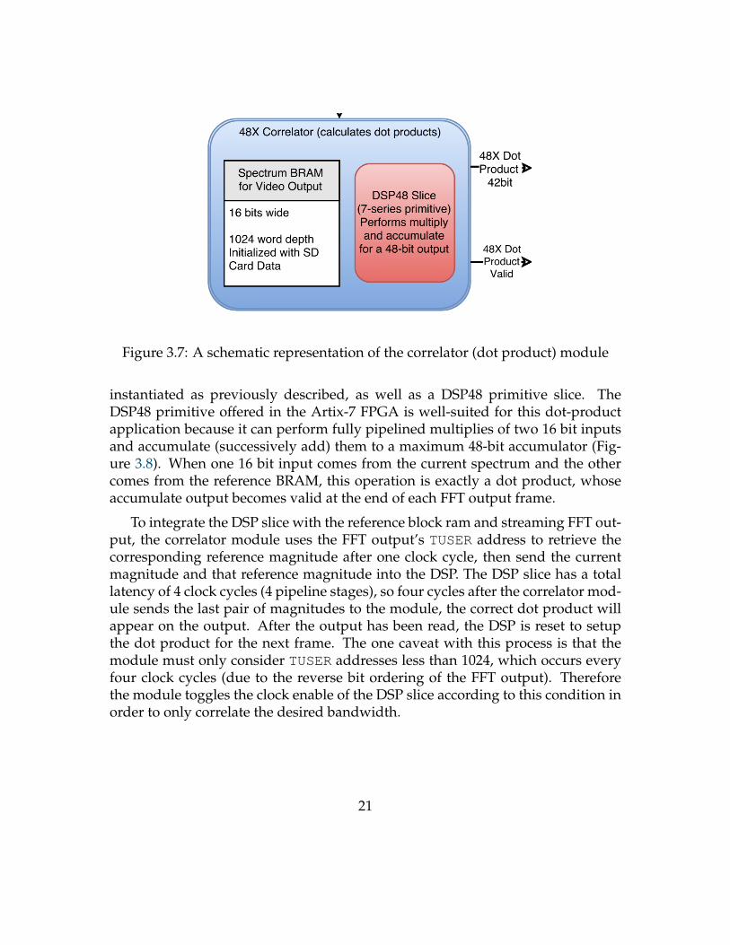
Figure 3.7: A schematic representation of the correlator (dot product) module

instantiated as previously described, as well as a DSP48 primitive slice. TheDSP48 primitive offered in the Artix-7 FPGA is well-suited for this dot-productapplication because it can perform fully pipelined multiplies of two 16 bit inputsand accumulate (successively add) them to a maximum 48-bit accumulator (Fig-ure 3.8). When one 16 bit input comes from the current spectrum and the othercomes from the reference BRAM, this operation is exactly a dot product, whoseaccumulate output becomes valid at the end of each FFT output frame.

To integrate the DSP slice with the reference block ram and streaming FFT out-put, the correlator module uses the FFT output’s TUSER address to retrieve thecorresponding reference magnitude after one clock cycle, then send the currentmagnitude and that reference magnitude into the DSP. The DSP slice has a totallatency of 4 clock cycles (4 pipeline stages), so four cycles after the correlator mod-ule sends the last pair of magnitudes to the module, the correct dot product willappear on the output. After the output has been read, the DSP is reset to setupthe dot product for the next frame. The one caveat with this process is that themodule must only consider TUSER addresses less than 1024, which occurs everyfour clock cycles (due to the reverse bit ordering of the FFT output). Thereforethe module toggles the clock enable of the DSP slice according to this condition inorder to only correlate the desired bandwidth.

21

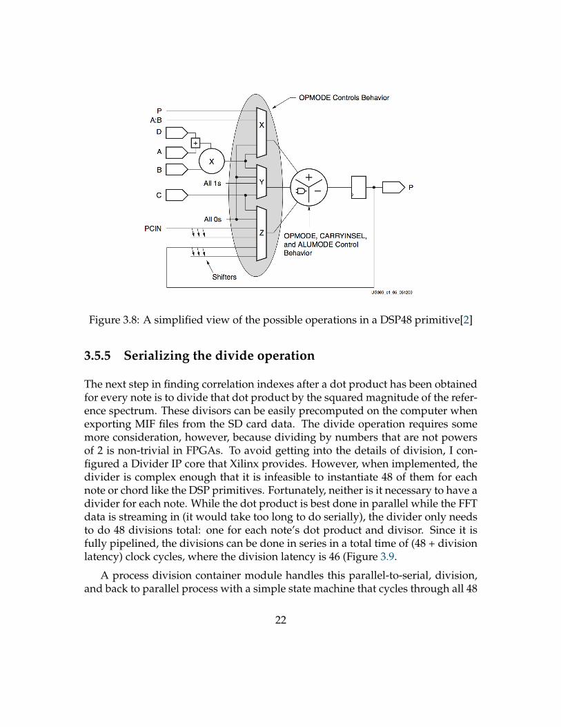
Figure 3.8: A simplified view of the possible operations in a DSP48 primitive[2]

3.5.5 Serializing the divide operation

The next step in finding correlation indexes after a dot product has been obtainedfor every note is to divide that dot product by the squared magnitude of the refer-ence spectrum. These divisors can be easily precomputed on the computer whenexporting MIF files from the SD card data. The divide operation requires somemore consideration, however, because dividing by numbers that are not powersof 2 is non-trivial in FPGAs. To avoid getting into the details of division, I con-figured a Divider IP core that Xilinx provides. However, when implemented, thedivider is complex enough that it is infeasible to instantiate 48 of them for eachnote or chord like the DSP primitives. Fortunately, neither is it necessary to have adivider for each note. While the dot product is best done in parallel while the FFTdata is streaming in (it would take too long to do serially), the divider only needsto do 48 divisions total: one for each note’s dot product and divisor. Since it isfully pipelined, the divisions can be done in series in a total time of (48 + divisionlatency) clock cycles, where the division latency is 46 (Figure 3.9.

A process division container module handles this parallel-to-serial, division,and back to parallel process with a simple state machine that cycles through all 48

22

Figure 3.9: A schematic view of the process division module’s operation

dot products and divisors, sending them into the divider core in series. The cor-relator modules that provide the dot product also assert a valid signal to indicatethat the process divider module can begin division. Similarly, the process dividermodule asserts its own valid signal when all of its divisions have completed.

One annoyance with actually implementing this process division module wasVivado’s refusal to allow unpacked bus arrays as input and output ports. Tomy knowledge, it appears that this functionality is specific to SystemVerilog, andwhile Vivado has support for many SystemVerilog features, it still does not allowunpacked array ports.

For example, I would have liked to have written the dot product inputs into theprocesd division module as follows: input [41:0] dot product [0:47].Because this wasn’t allowed, I chose to define a flattened, packed bus as input[47*48-1:0] dot product f and use 48 assign statements to map the un-packed array into the flattened bus, as follows:

assign dot_product_f[0*42 +: 42] = dot_product[0];





// ...etc

23

There is likely a more elegant solution to this problem (perhaps with a 2Dpacked array) but due to time limitations, I decided to stick with what workedand continue developing other modules.

All in all, the entire correlation calculation process reaches completion less than100 cycles after each FFT frame has finished outputting is frame of spectral data.Out of the 26,624 clock cycles between 4kHz samples, less than 4096+100 ≈ 4, 200of them are needed for correlation processing.

3.5.6 Processing and displaying correlation values

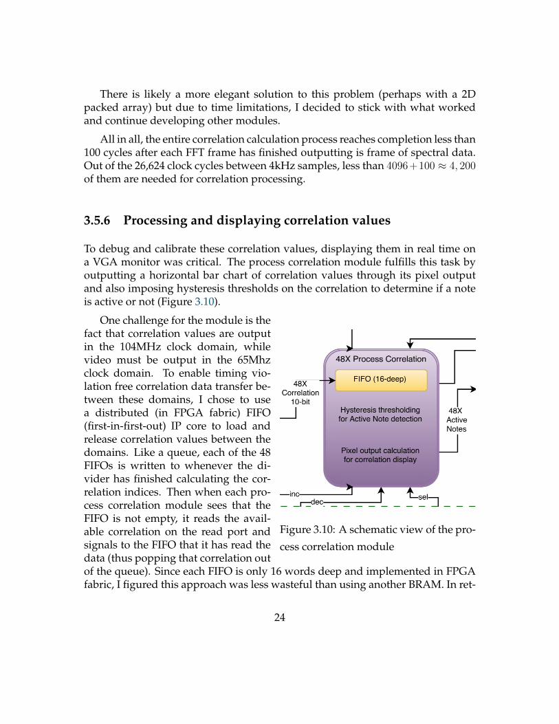
To debug and calibrate these correlation values, displaying them in real time ona VGA monitor was critical. The process correlation module fulfills this task byoutputting a horizontal bar chart of correlation values through its pixel outputand also imposing hysteresis thresholds on the correlation to determine if a noteis active or not (Figure 3.10).

Figure 3.10: A schematic view of the pro-

cess correlation module

One challenge for the module is thefact that correlation values are outputin the 104MHz clock domain, whilevideo must be output in the 65Mhzclock domain. To enable timing vio-lation free correlation data transfer be-tween these domains, I chose to usea distributed (in FPGA fabric) FIFO(first-in-first-out) IP core to load andrelease correlation values between thedomains. Like a queue, each of the 48FIFOs is written to whenever the di-vider has finished calculating the cor-relation indices. Then when each pro-cess correlation module sees that theFIFO is not empty, it reads the avail-able correlation on the read port andsignals to the FIFO that it has read thedata (thus popping that correlation outof the queue). Since each FIFO is only 16 words deep and implemented in FPGAfabric, I figured this approach was less wasteful than using another BRAM. In ret-

24

rospect, I realize that using a single 48-word BRAM is not bad at all, and rollingmy own synchronize module would likely be most efficient. Nevertheless, I en-joyed the opportunity to learn how FIFOs work.

Once the latest correlation value has been retrieved from the FIFO, the processcorrelation module performs an integratino step using an exponential moving av-erage (also inspired by 6.02), which is a form of simple low-pass filtering that takesthe following form:

filtered correlation = α(latest correlation) + (1− α)(last filtered correlation)

In practice, I settled with an α value of 132

, but even with the filter, I felt therewas a lot of room for improvement. (See Ch. 5. Review and Lessons Learned)

Each process correlation module also determines whether its note is active ornot according to its hysteresis rules. If its filtered correlation value is greater thanthe inactive-to-active threshold, the note becomes active. Then, to become inac-tive, the correlation must drop to below the lower active-to-inactive threshold.This helps to alleviate the rapid fluctuations in value that the correlations experi-ence.

To calibrate these hysteresis thresholds, the module offers increase, decrease,and threshold selection inputs, which allowed simple calibration of thresholdsin using the buttons on the Nexys 4 board. This feature was very useful for us tocalibrate each note’s ideal thresholds experimentally and rapidly. Once we arrivedat the best thresholds, we could read them off the hex display and override theirinitial values using parameters as necessary.

Finally, each process correlation module outputs its correlation value in videoformat by taking in hcount and vcount values from an XVGA module and out-putting the appropriate pixel value at that position. This process is very similar tothe spectral histogram video module, but with the addition of displaying upperand lower hysteresis bounds in video.

3.6 Serializing active notes

The last task for the audio processing design is to pass on the active note data tothe game logic Nexys for scoring. Once again, there was an inter-clock domain

25

challenge, as the active note data is in the 65Mhz domain, but the serialized datashould be in the 100Mhz clock domain, as that is the frequency at which the gameNexys scores note data. Once again, I used a distributed FIFO to transfer the 48bit wide active note bus across domains. Once in the 100Mhz domain, a serializermodule uses an internal counter to output the active notes serially over a dataline, while asserting the sync line at the end of every data packet. Each packet wasdivided into 64 time segments that are each 8,192 clock cycles wide. The first 48of these segments are the only meaningful ones, and the serial position of them inthe packet represents the index of an active note. Such a slow rate was necessarybecause over the approximately 70cm length of wire connecting the Nexys 4’s,high frequency pulses tend to deterioriate significantly, resulting in overflow of apulse into neighboring time segments.

3.7 Testing the audio processing modules

In the process of testing several modules in the audio processing component, thesimulation features integrated into the Vivado Design Suite were often helpful.For example, when testing the SD card saving module’s state machine, the simu-lator’s waveforms helped me realize that I had misinterpreted the form that oneof Jono’s SD Card Controller outputs. The ready for next byte signal was actu-ally high for eight clock cycles at a time rather than 1 clock cycle per byte as I hadpresumed. Figure 3.11 shows a simulation of the SD saving module in Vivado.

Figure 3.11: A logic waveform from a simulation of the SD saving module

Even more useful than the simulator tools was the Integrated Logic Analyzerfeature available as a synthesizable IP core in Vivado. Essentially, the IP core im-

26

plemented its own mini logic analyzer for a user configurable set of probes withinthe FPGA fabric itself. Then, in the Vivado hardware manager, one can configurecustom triggers for capturing logic frames of varying widths of all the probe lines.This was a lot easier than assigning a small number of probes to the PMOD portsand then fiddling with actual logic analyzer probes to capture the right frame.In fact, it was often easier to simply drop in an ILA core where a module wasnot working properly than to write a test bench module and simulate the design,which took significant time and was not guaranteed to be 100% accurate. The ILAwas not without a cost, however; the core itself added significant time to the im-plementation of a design and also occupied a lot of space within the FPGA fabric.

27

4. Game Processing Implementation

4.1 Overview of overarching design decisions - Ryan

While it was unclear for a while whether the audio side should utilize the Nexys4or the 6.111 labkit, it was clear from the beginning that the Nexys4 would be thecorrect choice for the game side. It’s 12 bit VGA and PWM audio were suitable forthe game’s AV needs, and the built in hardware for interfacing with an SD cardwas necessary. Additionally, the amount of memory available was essential forstoring large graphics assets and portions of song data.

From the beginning of the design stage, I had a desire to draw a large numberof abstractions around portions of the game, to make each abstraction level verysimple and easy to understand (Figure 4.1). I eventually realized that this was ac-tually a complete pain, once new interconnections needed to be added and testingneeded to be done. I suppose one of the most important things I got out of thisproject was the understanding that Verilog is hardware, not software, and I needto forget most of the things I know about writing software in order to be effectivein writing HDL for FPGAs.

28

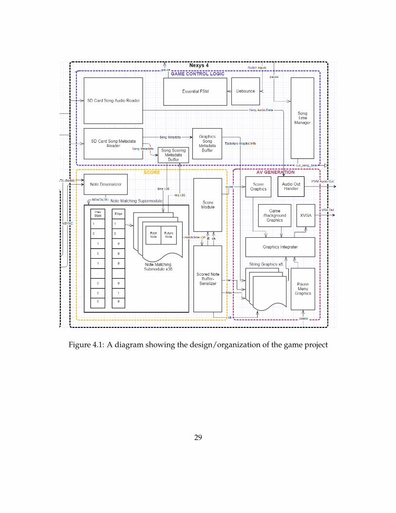
Figure 4.1: A diagram showing the design/organization of the game project

29

4.2 Game control logic - Ryan

4.2.1 Song time

The Control Logic block maintained the global song time value, which was a 16-bit value that incremented every 10ms (1,000,000 clock cycles at 100mhz). This al-lowed for a song time time of up to 11 minutes, which was decided to be enough,and a note resolution of 10ms, which is also a very reasonable resolution, sincetiming differences of less than 1/100th of a second are essentially indistinguish-able to humans. The designation for song time to be 16-bits also made the storagein the SD card exactly 2 bytes per note time, which is convenient. This valuestopped incrementing when the game was paused, and was set back to 0 when areset signal was applied.

4.2.2 Simple FSM

Also in the Control Logic block was a simple FSM which took debounced inputsfrom the Nexys’ buttons and switches and paused or reset the game accordingly.It originally also made sure the game did not progress until the metadata andaudio was loaded, but this was dropped with the SD card functionality, becausethere was no longer anything to load. More on the SD complications below.

4.3 Metadata loading - Ryan

4.3.1 Overview of Metadata

In the context of this project, metadata refers to the information about a song thatcorresponds to the guitar part that needs to be played. A single ”piece” of meta-data contains a pitch index (out of the 37 pitches we were detecting), a string (outof 6) and fret index (out of 17), which are necessary because a single pitch can beplayed in several string/fret combinations on a guitar (we needed to pick one torender on the screen–playing any one of them was indistinguishable to us, and

30

also to anyone listening to the guitar, but there is usually one that is most conve-nient), and finally a 16-bit time value that represented what time in the song thatshould ideally be played (Figure 4.2).

Figure 4.2: A diagram showing the various places a single pitch can be played on

a fretboard. Equivalent pitches have the same letter and color.

As far as storing metadata on the SD card was concerned, 4 bytes/word wereneeded (16 bits for time, 6 for pitch, 3 for string, 5 for fret, and 2 extra to make thetotal divisible by 8). The extra 2 bits could be used to signify whether or not theword was the end of the song (2’b00 for continue reading, and 2’b11 for End OfFile). Additionally, 4 was a good number of bytes, due to it dividing evenly into512 bytes, which was how much data the SD card controller we were using wouldread at a time.

The scoring block needed to know what note was being played, and when,so that it could compare that to the data it was receiving from the audio Nexysand score it appropriately. Meanwhile, the AV block needed to know when anote would be played, and the fret/string combination for that note, so that itcould render a correctly numbered sprite on the right string, and such that whensong time was the time when the note should be played, the sprite would be pass-ing directly over the ”Play Now!” bar on the screen.

4.3.2 Utilization of BRAMs

A very serious design problem was the issue of getting metadata from a singlesource to be utilizable/sortable by several different components of the game sys-

31

tem. The scoring system needed the metadata to be in time-order after beingseparated by note, while the graphical interface needed the metadata to be sepa-rated by string before being sorted in time-order. A lot of time was spent figuringout how to have multiple different access schemes into this data table such thatall of this information was available within a clock cycle or two for the modulesthat needed it. Eventually, in an effort to have a working and demonstrable prod-uct for the checkoff, I gave up on this pursuit and hardcoded the metadata for asimple song (Mary Had a Little Lamb–which was also desirable for gently testingthe note-detection functionality due to it only having 4 different pitches, none ofwhich were played simultaneously) into a few BRAMs that were contained withinthe modules that needed the data.

In retrospect, it is very unfortunate that this was only done as a last resort,because after I did it I realized that the memory allowance of a Nexys was far morethan I had previously thought. Rather than have a single data storage with a veryconvoluted interface for getting the results I wanted, I actually had the BRAMallowance available on the device to just have a copy of all relevant data in eachmodule that needed it. That just seemed like an approach that was so inefficientthat I didn’t figure the hardware allowance would be enough for it. Because I wasunable to create a reliable interface into a singular table, I had to throw it out forthe sake of the project, and with it the SD card functionality. However, with thisdistributed memory scheme, implementing the SD card functionality would’vebeen relatively simple, with each word being broken up into it’s relevant piecesand then written to the particular metadata buffer that needed it. My biggestregret in this project was probably not realizing this sooner, and just keeping myapproach simple, because I had to throw out a lot of project potential with it whenI finally compromised and went with the simple distributed approach, and nolonger had the time to piece it all together again.

4.4 Scoring - Ryan

4.4.1 Parallel matching (37x)

Actual matching of notes was handled by 37 individual pitch-matching modules.Each module stored the most recent time that had already passed for which it’spitch should have been played, and the most recent time for which the should

32

pitch be played which hadn’t occurred yet.

The parent module stored a 1-cycle history of note-states was saved, such thata match would only be triggered on the rising edge of a note.

When a match for this pitch occurred, this module received a trigger and thencompared the current song time to the stored times for the past and future note,and returned whichever one was closer to the current time. Each of the 37 moduleshad a 16-bit time bus plus an enable line to the buffer-serializer, and whichevertime was chosen was sent along to the buffer-serializer, along with an enable trig-ger.

4.4.2 Parallel metadata request

Each pitch module also had a 16-bit time bus plus a request’ and available’ lineto the metadata controller. If the future note was written invalid in the module(either by being matched, or by becoming older than the current song time andbeing shifted into the past note slot) then the module would set the request linehigh. Eventually the metadata controller would set the available line high, atwhich point the new future time was available on the 16-bit bus, and the modulecould set its request line back to low and write in the new note.

As I mentioned above, with a distributed BRAM module the pitch modulewould’ve had an entire BRAM for metadata, and would not need to interface witha controller except at the loading of a song, during which time the SD controllerwould write into the pitch module’s BRAM all notes that matched it’s pitch, aswell as their time. Then the pitch module would pull metadata from it’s internalmemory as needed instead of interfacing with an external controller.

4.4.3 Serializing parallel-matching results

The buffer-serializer module was a critical piece of the scoring functionality, tak-ing information from a myriad of pitch module busses, and outputting a singlebus into the score module, and a few into the AV string modules (these renderedthe note-sprites on the screen–more on them later). It played a key part in coordi-nating the efforts of many small, disconnected pieces of the project.

This module worked by checking the match triggers from the pitch modules. If

33

any were high, it would take the highest pitch that was active, compare it’s matchtime to the current time, and calculate the absolute value of the difference, whichit sent off to the score module as an indication of how accurately the note wasplayed. With this pitch, it also sent a trigger to the graphics module correspondingto each string where that note could be played, along with the fret value on thatstring where it could’ve been played. It also sent the note’s correct time to thestrings, such that each string had all the information it needed to match the notematched to one of its sprites (more on how these modules worked later).

The decision to place priority on the highest pitch that matched was arbitrary,but motivated by the need to simplify the problem at the cost of being unableto match two notes in the same clock cycle. Without making this compromise,we would’ve either needed to have far more interfacing with the neighboringmodules, or have some queueing of note-matches. This was determined to be notworth the complication, as the probability of two note-matches occurring on thesame 100mhz clock cycle are negligibly small.

4.4.4 Score Tabulation

The scoring module graded on a roughly exponential scale. If a note was playedwithin 100ms of it’s intended time, the score would be incremented by 100. Sim-ilarly, accuracy within 250ms would be awarded 50 points, within 500ms wouldbe awarded 25 points, and within 1s would be awarded a measly 10 points. Any-thing beyond that would not receive any points.

4.4.5 Testing scoring

Throughout the implementation process, the scoring portion received the mostthorough testing, due to its relative non-reliance on other pieces of the game. Testbenches were written for each component and simulated in Vivado Design Suite.Later, when the rest of the game project was in a more put-together state, an Inter-nal Logic Analyzer (from Vivado’s IP catalog) was synthesized with the project,and made sure that the behavior of the scoring was still correct when actuallyimplemented.

Additionally, since the note recognition was not in a usable state for the ma-jority of the testing and integration stage, an AI guitar player’ was implemented,

34

which simply proceeded through the 37 pitches and set each one high for a singleclock cycle, such that it would never miss a note. While this AI scored terribly(playing each note as early as physically possible, and only earning 10 points eachtime), it made testing of the scoring functionality (and later, the graphics as well)very straightforward.

4.5 Graphics generation - Mitchell

4.5.1 Compressing a high quality background image to fit in BRAM

For the high-quality game graphics, we wanted to create an environment akin tothe original Guitar Hero games, where a crowd in the background helps foster theimpression that the player is entertaining an audience. We also wanted to displaygraphics that were a notch above typical FPGA graphics that are limited to fewcolors and low resolution. I decided that the most efficient way to do this wasto develop one large background image rather than isolate the game title, gui-tar strings, background, and crowd into separate sprites (Figure 4.3. This wouldlower complexity on the FPGA side and save time, since outside of note sprites,the game is fairly static.

Without involving the DDR3 memory and the world of memory controllersand frame buffers, the main challenge with displaying such a large image is stor-age space within the FPGA. If one were to store the entire 1024x768 image at 12-bitcolor, one would need roughly 260 36Kbit BRAM36 primitives, far greater thanthe 135 available on the Artix 7 100T. However, with the background image wewanted to display, there as a high degree of regularity, or predictability in the pixeldata. For example, more than half of the background image is a solid, continuousbackground color. This lower entropy in the image was an easy opportunity toemploy some compression strategies to reduce the number of BRAMs required.

In 6.02, I learned a variety of compression techniques, some more efficientthan others. While using a Hamming code for the pixel data or LZW compres-sion would have yielded higher compression ratios, I chose a much simpler toimplement compression techinique: pixel run length. Essentially, at a certain ad-dress, the BRAM’s corresponding word contains the pixel color value, but also afixed-length value that indicates how many of the following pixels are identical.Because the background image largely consists of continuous runs of the same

35

Figure 4.3: The desired background image for the game

color, this approach can yield an effective compression ratio.

Another observation is that the color palette of the background image couldbe reduced to only a few colors without compromising the output quality to anobservable degree. With full 12-bit RGB color, there are a total 216 = 4096 colors.However, by reducing the color palette of our image in GIMP to 62 colors, nearlyidentical quality could be achieved with much less information storage.

In order to support the reduced color palette, the image has to be stored inindexed color format rather than 12-bit RGB format. The difference is that eachpixel has an associated 6-bit index into a shared color palette table, rather than a12-bit RGB value. That index is then used to look up the actual 12-bit color fromthe color palette table, at the expense of one extra clock cycle of latency.

36

To implement both run length compression and indexed color, I used a com-bination of the GIMP photo editing tool and a Python script. GIMP was used toadjust the image to my liking and reduce the color palette to 62 colors that bestrepresented the image. Then, with the help of the PIL python image processinglibrary, I iterated through every pixel in the image and created .coe files for twotables: a run table and a color lookup table. With some iteration, I found that thebest fixed bit length to encode run length was 2 bits, which covers run lengthsfrom 1 to 4 repeated pixels. If a run was more than four pixels, a new run wouldhave to be started for each set of four identical pixels.

An entire word in the run table was thus 8 bits total: the first two bits wouldencode the run length, and the last six bits would index into the color lookuptable. In the end, the image was reduced to around 2Mbits of data, a significantimprovement compared to 9Mbits had it been uncompressed. When initializedinto BRAM primitives, the run table takes up 62 BRAMs, less than half of the135 total, which left plenty for the rest of the game graphics and metadata. Thecolor lookup table was relatively small (64 words deep), so it was implemented asdistributed memory instead.

4.5.2 Generating Note Sprites

Compared to configuring the background images, the note sprites were relativelysimple to configure. Each sprite was 32x32 in resolution, so they could each fiteasily uncompressed in a 13 bit wide by 1024 word deep BRAM18 primitive. (Therationale for having a 13th bit is detailed in the following graphics rendering sec-tion). Each sprite was again created in GIMP, with 18 versions with the num-bers 0-17 on them corresponding to all possible fret positions. Because there weremany of them, I again took the approach of instantiating the sprite brams usingthe $readmemh function, Python-generated MIF files, and inferred BRAMs. Thistime, instead of spectrum data, the MIF files would contain raw RGB values:

37

4.6 Graphics Rendering - Ryan

4.6.1 Integrating graphics and the alpha bit approach

The entire graphical interface could be split into a set of layers, with a certainpriority such that if two layers wrote a pixel to the same location, the pixel fromthe layer with higher priority would be rendered. Whether or not a layer hadwritten a pixel was determined by adding a 13th alpha’ bit (onto the 12 bit RGBvalue) to the front of the signal, which was 1 if the pixel was to be rendered, and 0if the layer was transparent at that location. More complicated alpha integrationwas unnecessary, because there was no reason to support partial opacity. This setof layers went as follows:

• Pause MenuThis layer had the highest priority because if the menu were ever being ren-dered it would need to cover all of the game pieces underneath it. For pre-liminary testing this menu was a simple grey rectangle which rendered ifthe game was paused. As checkoff approached, there wasn’t much time tomake a prettier pause menu, and so this was eventually replaced by a filterthat inverted every pixel on the entire screen to photonegative if the gamewere paused. This made it more clear that the game was paused, and lefteverything visible while the game was paused, which was a nice plus.

• ScoreThis module would display the decimal score in a nice font on the upper-right side of the screen. This was cut due to time, as implementing anotherset of sprites and converting from binary/hex to decimal is a nontrivial mat-ter. The score is instead displayed in hex (along with the current song time)on the segmented display on the Nexys board.

• Strings 6 through 1Each string module handled the rendering of the fret sprites onto the string(which was actually in the background layer), and moved the sprites suchthat they passed play at the proper time, timed-out, and also changed colorsupon being matched. More on that later.

• BackgroundThis layer rendered the background image, and had no alpha bit because it

38

was the lowest layer, and needed to provide an RGB value for every pixellocation.

4.6.2 Parallel sprite table access

It was arbitrarily decided that strings should render a maximum of 5 fret spriteseach, which should be enough for most songs. In retrospect, making that num-ber higher, like 10-15, might’ve been preferable, but it worked just fine for ourpurposes. This made the maximum number of fret sprites 30. The problem in-troduced by this was that there were 18 sprites to draw from BRAMs (for frets0-17), so there could only reasonably be a single set of sprite lookup tables. Thismeant that a coordination scheme needed to be used to ensure that all 30 couldcooperatively look into the table.

This problem was solved by only giving a single sprite handler control overthe address into the memory for the read at a single time. This was determinedby whether or not a sprite were present at any particular pixel, which requiredthe easily-enforceable invariant that no two sprites would overlap. If a particularclock cycle fell into a sprites domain, it could decide the memory address, and allother sprites would return a string of 0’s for their address. Then, all of the spritehandlers’ address bits were bitwise OR’d, which produced the final address.

Another problem resulting from having a single coordinated memory accessamong all sprite handlers was that sprite handlers weren’t assigned the same fretvalues, and as such needed to look at different tables. This problem was solvedby having a single read of the memory return the pixel values for all of the sprites(for a particular pixel location on the sprite). All of the sprite handlers were privyto this single output, and indexed into it according to their fret value.

One final problem with sprite lookup, unrelated to the parallel access issues,was the fact that BRAMs take a clock cycle to look up the necessary data once theaddress is asserted. This means that there would need to be an additional clockcycle between calculating the address and receiving the data that was requested.Instead of pipelining to resolve this, I simply clocked the BRAMs at 130 mhz, sothat the additional clock cycle occurred during the low portion of the 65 mhz clockthat the rest of the graphics ran on.

39

4.6.3 Matching sprites

When a match occurred, all of the string modules received the time of the match,as well as the fret that the note would’ve been on their string (if applicable–eachstring cannot play every pitch). The matching occurred by checking all of thecurrently rendered sprites for a sprite that had a time and fret that matched theinformation received. If there were one, it’s state was set to matched’ and thesprite would be inverted to provide a visual indication that the note was scored.

40

5. Review and Lessons Learned

5.1 Mitchell

Overall, I’m happy with how the project turned out. I learned a lot about us-ing interesting features in modern FPGA tools, and also made many connectionsacross different subjects such as Fourier transforms and employing compressiontechniques in hardware. I was pleasantly surprised with the amount of overlapbetween the class and subjects such as 6.004 (computational structures) and 6.02(digital communcation systems). A large part of my goals in taking this classwere to learn digital hardware design (which is hard to learn by oneself withjust the internet) and experiment with working in the frequency domain. I feltthis project was a great way to achieve both of those goals and also gain a broadknowledge about how previously magical, high frequency digital devices work attheir fundamental level. After doing this project, I feel like I’m in a better positionto understand how digital boards such as oscilloscopes, computer motherboards,or smartphone boards operate, which is something I have always been curiousabout.

If I were to continue work on the project, some things that definitely needadjustment are the FFT frame size, correlation formula, and correlation low-passfiltering.

The issue with the FFT frame size is that with 4096 samples per frame anda 4KHz sample rate, a given stimulus’s frequency content stays in the frame forapproximately 1 second. This means that the system does not decay spectral peaksquickly enough, which greatly hinders the ability to play the same note manytimes in succession. WIth hysteresis on the correlation values, it is likely that thesecond time one plays the same note, it will still be active from the previous time

41

it was played. I experimented briefly with some approaches for shortening thedecay time such as only passing samples for a subset of the frame to the FFT orpassing a repeated subset of the samples several times in one frame. However,in both cases the output spectrum contained undesirable components due to thenature of the technique. To arrive at a solution, I would likely need to take adeeper look at how what effects the sample frame has on fourier transforms.

The correlation formula is also still far from perfect because when it is scaledby the ratio of the current spectral magnitude to the reference spectral magnitude,the current spectral magnitude drops out of the expression. This is a problembecause notes played on the lower strings of the guitar are significantly higherenergy and contain more harmonic content in the frame. Therefore they have verylarge magnitudes, which results in large dot products regardless of how similarthe vectors are, which results in nearly every note becoming active. I think theoptimal correlation expression would be some combination of the original cosineof the vector expression and a penalty for very low spectral magnitudes so thatthe current spectral magnitude term stays in the expression.

Finally, the use of an exponential weighted moving average filter for low-passfiltering the correlation indices has experimentally been not ideal and still resultsin rapid fluctuations that the hysteresis even has trouble compensating for. Givenmore time, I would experiment with an FIR filter as used in Lab 5 of the class toprovide a more ideal low-pass filter.

5.2 Ryan

My biggest regret/learning experience resulted with not sticking to the mantra of”Keep it Simple, Stupid” in regards to the storage and distribution of metadata.After the fact, distributed storage of metadata is a very appealing concept andwould’ve made reading/handling data from the SD card very, very straightfor-ward.

I also learned a lot about the usefulness of IPs (procedurally generated mod-ules, essentially) and the Vivado IP catalog. I wish I had come into this projectknowing how useful they are, because reinventing the wheel in regards to genericVerilog functionality is a largely wasteful endeavor. The Block Memory Wizard,Clock Wizard, and the Internal Logic Analyzer all made my life a lot easier overthe course of implementation, and perhaps if I’d known how IPs worked from the

42

start, I would’ve made more design decisions around the idea and had an easiertime.

As a general philosophy regarding HDLs and FPGAs, I feel like I learnedto stop treating Verilog like software. Abstractions are only good if they neatlycompartmentalize functionality with a minimal amount of outside influence, andkeeping the number of abstractions in a project down is extremely handy. Other-wise they become a serious pain to maintain over the implementation of a project.

Overall, I’m happy with results of this project. I’m sad that not all of it wentaccording to plan, and there are still bugs present, but I think that is in the natureof picking an ambitious project and learning a lot on the go. I feel like this projectgave me a much better feel for how large-scale Verilog development works, andhow to better get what I want out of an FPGA in a timely fashion, much moreso than I feel the labs had. The working product, though not as glamorous asimagined, is very close to the goals we set for this project, which in hindsight isquite a satisfying accomplishment.

43

6. Conclusion

Guitar Hero Fast Fourier Edition has proved to be a challenging, yet rewardingendeavour for us to learn digital hardware design and extend our shared interestin playing guitar. The project came close to achieving all its main goals, such asguitar note recognition, serialization and deserialization between Nexys boards,note matching and scoring, and advanced game graphics. Due to the complexityof the project, we did not have nearly the amount of time we would have liked forintegration and testing of all the parts, but we were very happy with how muchintegration we did achieve by project checkoff time. If given more time, we feelthat we could bring the project to the level of an entertaining, polished productfeaturing more accurate note recognition, proper note sprite matching for poppingplayed notes off the display, loading of song audio and metadata from and SDcard, and display of the score on the VGA display. Despite these shortcomings,the concepts we’ve learned throughout the project’s challenges have been veryrewarding and inspire us to explore the FPGA world further. We are also excitedby the prospect of similar note recognition technologies using actual instrumentsspreading throughout the Guitar Hero and interactive music game genre.

44

References

[1] Fast Fourier Transform v9.0 Product Guide. (2015, Sep. 30). Xilinx [Online].Available:http://www.xilinx.com/support/documentation/ip documentation/xfft/v9 0/pg109-xfft.pdf

[2] 7 Series DSP48E1 Slice User Guide. (2014, Nov. 10). Xilinx [Online]. Available:http://www.xilinx.com/support/documentation/user guides/ug479 7Series DSP48E1.pdf

45

Appendices

46

A. Source files

All source files, IP configurations, block designs, memory initialization files, andbitstreams for both the audio and game Vivado projects in addition to suppoortingpython scripts are available at Github.

47

http://github.com/mitchgu/GuitarHeroFFE

final project report -...

Documents