filtering and enhancing images
TRANSCRIPT

Chapter 5
Filtering and Enhancing Images
This chapter describes methods to enhance images for either human consumption or for fur-
ther automatic operations. Perhaps we need to reduce noise in the image; or, certain image
details need to be emphasized or suppressed. Chapter 1 already introduced two methods of
image �ltering: �rst, in the blood cell image, isolated black or white pixels were removed
from larger uniform regions; secondly, it was shown how a contrast operator could enhance
the boundaries between di�erent objects in the image, i.e. improve the constrast between
the pictures and the wall.
This chapter is about image processing, since the methods take an input image and create
another image as output. Other appropriate terms often used are �ltering, enhancement, orconditioning. The major notion is that the image contains some signal or structure, which
we want to extract, along with uninteresting or unwanted variation, which we want to sup-
press. If decisions are made about the image, they are made at the level of a single pixel or
its local neighborhood. We have already seen how we might label an image pixel as objectversus background or boundary versus not boundary.
Image processing has both theory and methods that can �ll several books. Only a few
classical image processing concepts are treated here in detail. Most methods presented use
the important notion that each pixel of the output image is computed from a local neigh-
borhood of the corresponding pixel in the input image. However, a few of the enhancement
methods are global in that all of the input image pixels are used in some way in creating
the output image. The two most important concepts presented are those of (1) matchingan image neighborhood with a pattern or mask (correlation) and (2) convolution, a single
method that can implement many useful �ltering operations.
5.1 What needs �xing?
Before launching into the methods of this chapter, it's useful to review some of the problems
that need them. Two general categories of problems follow.
1

2 Computer Vision: Mar 2000
Figure 5.1: (Left) Scratches from original photo of San Juan are removed; (center) inten-
sities of house photo with dark areas are rescaled to show better detail in some regions;
(right) image of airplane part has edges enhanced to support automatic recognition and
measurement.
5.1.1 An Image needs Improvement
� On safari in Africa you got a shot of a lion chasing an antelope. Unfortunately, the
sun was behind your main actor and much of your picture is too dark. The picture
can be enhanced by boosting the lower intensities and not the higher ones.
� An old photo has a long bright scratch, but is otherwise �ne. The photo can be
digitized and the scratch removed.
� A paper document needs to be scanned and converted into a text �le. Before apply-
ing character recognition, noise pixels need to be cleaned from the background and
dropouts in the characters need to be �lled.
5.1.2 Low-level features must be detected
� 0.12 inch diameter wire is made by a process that requires (closed loop) feedback
from a vision sensor that constantly measures the wire diameter. The two sides of the
wire can be located using an edge operator which accurately identi�es the boundary
between the wire and its background.
� An automatic pilot system for a car can steer by constantly monitoring the white lines
on the highway. The white lines can be found in frames of a forward-looking video
camera by �nding two edges with opposite contrast and similar direction.

Shapiro and Stockman 3
Figure 5.2: (Left) Original sensed �ngerprint; (center) image enhanced by detection and
thinning of ridges; (right) identi�cation of special features called \minutia", which can be
used for matching to millions of �ngerprint representations in a database (contributed by
Shaoyun Chen and Anil Jain).
� A paper blueprint needs to be converted into a CAD (computer-aided-design) model.
Part of the process involves �nding the blueprint lines as dark streaks in the image
about 1 pixel wide.
This chapter deals mostly with traditional methods of image enhancement and somewhat
with image restoration. Before moving on, it is important to de�ne and distinguish these
terms.
1 Definition Image enhancement operators improve the detectability of important im-age details or objects by man or machine. Example operations include noise reduction,smoothing, contrast stretching, and edge enhancement.
2 Definition Image restoration attempts to retore a degraded image to an ideal condi-tion. This is possible only to the extent that the physical processes of ideal image formationand image degradation are understood and can be modeled. The process of restoration in-volves inverting the degradation process to return to an ideal image.
5.2 Grey level mapping
It is common to enhance images by changing the intensity values of pixels. Most software
tools for image processing have several options for changing the appearance of an image
by transforming the pixels via a single function that maps an input grey value into a new
output value. It is easy to extend this so that a user can indicate several di�erent image
regions and apply a separate mapping function to each. Remapping the grey values is often
called stretching because it is common to stretch the grey values of an image that is too
dark onto the full set of grey values available. Figure 5.3 shows a picture whose intensity
values are stretched according to four di�erent mapping functions. Figure 5.3(a) shows the
result of applying an ad hoc function, which was designed by the user of an interactive
enhancement tool. The user de�nes the grey level mapping function gout = f(gin) using
the computer mouse: typically the image tool �ts a smooth spline through points chosen
by the user. Figure 5.3(b) and (c) show remapping using the function f(x) = x1= : this
function nonlinearly boosts or reduces intensities according to whether > 1 or < 1.

4 Computer Vision: Mar 2000
0 1
1
gin
gout
0 1
1
f(x) = x0.3
gin
gout
0 1
1
f(x) = xg
in
gout
20 1
1
gin
gout
t
=x 5
f(x)=x0.5
0
500
1000
1500
2000
0 50 100 150 200 250
Histogram: bins 0-255
’house.hist.gnu’
0
500
1000
1500
2000
0 50 100 150 200 250
Histogram: bins 0-255
’house.hist.gnu’
0
500
1000
1500
2000
0 50 100 150 200 250
Histogram: bins 0-255
’house.hist.gnu’
0
500
1000
1500
2000
0 50 100 150 200 250
Histogram: bins 0-255
’house.hist.gnu’
(a) (b) (c) (d)
Figure 5.3: (Top row) Intensity mapping functions f and (center row) output images re-
sulting from applying f to the original image from Figure 5.1 and (bottom row) resulting
grey level histograms. (a) House image pixels remapped according to a user-de�ned smooth
function that stretches the low range of intensities and compresses the higher range ; (b)
Gamma correction with f(x) = x0:3 boosts dark pixels more than bright ones; (c) Gamma
correction with f(x) = x2:0 reduces bright pixels more than dark pixels; (d) Use of two
di�erent Gamma values to boost dark pixels < t and reduce bright pixels > t. Di�erent
scene objects appear with di�erent clarity in the several images.
This operation ( called Gamma correction) might be the proper model to restore an image
to an original form after undergoing known physical distortion. Figure 5.3(d) shows that
a more complex mapping can be de�ned by using di�erent functions for darker pixels and
brighter pixels according to some de�ning threshold t. All of the functions in Figure 5.3
stretch or extend at least some range of intensities to show more variation in the output.
Image variation will be increased in the intensity ranges where the slope of function f(x) is
greater than 1.
3 Definition A point operator applied to an image is an operator in which the outputpixel is determined only by the input pixel, Out[x; y] = f(In[x; y]): possibly function f
depends upon some global parameters.

Shapiro and Stockman 5
Figure 5.4: Histogram equalization maps the grey scale such that the output image uses the
entire range available and such that there are approximately the same number of pixels of
each grey value in the output image: images after histogram equalization are at the right.
4 Definition A contrast stretching operator is a point operator that uses a piecewisesmooth function f(In[x; y]) of the input grey level to enhance important details of the image.
Because point operators map one input pixel to one output pixel, they can be applied to
an entire pixel array in any sequential order or can be applied in parallel. Ad hoc mappings
of intensities, including nonmonotonic ones as in Figure 5.3, can be very useful in enhancing
images for general human consumption in graphics and journalism. However, in certain
domains, such as radiology, one must be careful not to alter a meaningful intensity scale to
which human experts and intricate sensors are carefully calibrated. Finally, we note that the
performance of some algorithms for machine vision might not be changed by monotonic grey
scale stretching (f(g2) > f(g1) whenever grey level g2 > g1), although humans monitoring
the process might appreciate the enhanced images.
5.2.1 Histogram equalization
Histogram equalization is often tried to enhance an image. The two requirements on the
operator are that (a) the output image should use all available grey levels and (b) the
output image has approximately the same number of pixels of each grey level. Requirement
(a) makes good sense but (b) is ad hoc and its e�ectiveness must be judged empirically.
Figure 5.4 shows images transformed by histogram equalization. One can see that the
remapping of grey levels does indeed change the appearance of some regions; for example,
the texture of the shrub in front of the house is better de�ned. The face image had been
cropped from a larger image and the cropped window did not have many lower intensity
pixels. Requirement (b) will cause large homogeneous regions, such as sky, to be remapped
into more grey levels and hence to show more texture. This may or may not help in image
interpretation.
Requirements (a) and (b) mean that the target output image uses all grey values z =
z1; z = z2; : : : ; z = zn and that each grey level zk is used approximately q = (R�C)=n times,
where R;C are the number of rows and columns of the image. The input image histogram
Hin[] is all that is needed in order to de�ne the stretching function f . Hin[i] is the number
of pixels of the input image having grey level zi. The �rst grey level threshold t1 is found
by advancing i in the input image histogram until approximately q1 pixels are accounted

6 Computer Vision: Mar 2000
for: all input image pixels with grey level zk < t1� 1 will be mapped to grey level z1 in the
output image. Threshold t1 is formally de�ned by the following computational formula:
t1�1Xi=1
Hin[i] � q1 <
t1Xi=1
Hin[i]:
This means that t1 is the smallest grey level such that the original histogram contains no
more than q pixels with lower grey values. The k-th threshold tk is de�ned by continuing
the iteration:tk�1Xi=1
Hin[i] � (q1 + q2 + : : :+ qk) <
tkXi=1
Hin[i]:
A practical implementation of the mapping f is a lookup table that is easily obtained from
the above process. As the above formula is computed, the threshold values tk are placed
(possibly repetitively) in array T [] as long as the inequality holds: thus we'll have function
zout = f(zin) = T [zin].
Exercise 1An input image of 200 pixels has the following histogram: Hin =
[0; 0; 20; 30; 5;5;40;40;30;20;10;0;0;0; 0; 0]. (a) Using the formula for equalizing the
histogram (of 15 grey levels), what would be the output image value f(8)? (b) Repeat
question (a) for f(11). (c) Give the lookup table T [] implementing f for transforming all
input image values.
Exercise 2 An algorithm for histogram equalization
Use pseudocode to de�ne an algorithm for histogram equalization. Be sure to de�ne all the
data items and data structures being used.
Exercise 3 A histogram equalization program
(a) Using the pseudocode from the previous exercise, implement and test a program for
histogram equalization. (b) Describe how well it works on di�erent images.
It is often the case that the range of output image grey levels is larger than the range of
input image grey levels. It is thus impossible for any function f to remap grey levels onto
the entire output range. If an approximately uniform output histogram is really wanted, a
random number generator can be used to map an input value zin to some neighborhood of
T [zin]. Suppose that the procedure described above calls for mapping 2q pixels of level g
to output level g1 and 0 pixels to level g1 + 1. We can then simulate a coin ip so that an
input pixel of level g has a 50-50 chance of mapping to either g1 or g1 + 1.
5.3 Removal of Small Image Regions
Often, it is useful to remove small regions from an image. A small region might just be
the result of noise, or it might represent low level detail that should be suppressed from
the image description being constructed. Small regions can be removed by changing single
pixels or by removing components after connnected components are extracted.

Shapiro and Stockman 7
Exercise 4Give some arguments for and against \randomizing" function f in order to make the output
histogram more uniform.
1 1 1
1 0 1
1 1 1
)
1 1 1
1 1 1
1 1 1
;0 0 0
0 1 0
0 0 0
)
0 0 0
0 0 0
0 0 0
X X X
X L X
X X X
)
X X X
X X X
X X X
;X
X L X
X
)
X
X X X
X
Figure 5.5: Binary image of red blood cells (top left) with salt and pepper noise removed
(top right). Middle row: templates showing how binary pixel neighborhoods can be cleaned.
Bottom row: templates de�ning isolated pixel removal for a general labeled input image;
(bottom left) 8-neighborhood decision and (bottom right) 4-neighborhood decision.
5.3.1 Removal of Salt-and-Pepper Noise
The introductory chapter brie y discussed how single anomalous pixels can be removed
from otherwise homogeneous regions and methods were extended in Chapter 3. The pres-
ence of single dark pixels in bright regions, or single bright pixels in dark regions, is called
salt and pepper noise. The analogy to real life is obvious. Often, salt and pepper noise is
the natural result of creating a binary image via thresholding. Salt corresponds to pixels
in a dark region that somehow passed the threshold for bright, and pepper corresponds to
pixels in a bright region that were below threshold. Salt and pepper might be classi�cation
errors resulting from variation in the surface material or illumination, or perhaps noise in
the analog/digital conversion process in the frame grabber. In some cases, these isolated
pixels are not classi�cation errors at all, but are tiny details contrasting with the larger
neighborhood, such as a button on a shirt or a clearing in a forest, etc. and it may be that
the description needed for the problem at hand prefers to ignore such detail.
Figure 5.5 shows the removal of salt and pepper noise from a binary image of red blood
cells. The operations on the input image are expressed in terms of masks given at the
bottom of the �gure. If the input image neighborhood matches the mask at the left, then
it is changed into the neighborhood given by the mask at the right. Only two such masks

8 Computer Vision: Mar 2000
Figure 5.6: Original blood cell image (left) with salt and pepper noise removed and compo-
nents with area 12 pixels or less removed (right).
are needed for this approach. In case the input image is a labeled image created by use
of a set of thresholds or some other classi�cation procedure, a more general mask can be
used. As shown in the bottom row of Figure 5.5, any pixel label 'L' that is isolated in
an otherwise homogenous 8-neighborhood is coerced to the majority label 'X'. 'L' may be
any of the k labels used in the image. The �gure also shows that either the eight or four
neighborhood can be used for making the decision; in the case of the 4-neighborhood, the
four corner pixels are not used in the decision. As shown in Chapter 3, use of di�erent
neighborhoods can result in di�erent output images, as would be the case with the red
blood cell image. For example, some of the black pixels at the bottom left of Figure 5.5 that
are only 8-connected to a blood cell region could be cleaned using the 4-neighborhood mask.
5.3.2 Removal of Small Components
Chapter 3 discussed how to extract the connected components of a binary image and de-
�ned a large number of features that could be computed from the set of pixels comprising
a single component. The description computed from the image is the set of components,
each representing a region extracted from the background, and the features computed from
that region. An algorithm can remove any of the components from this description based
on computed features; for example, components with a small number of pixels or compo-
nents that are very thin can be removed. This processing could remove the small noise
region toward the upper right in the blood cell image of Figure 5.5 (top right). Once small
regions are culled from the description it may not be necessary, or possible, to generate the
corresponding output image. If an output image is necessary, information must be saved in
order to return to the input image and correctly recode the pixels from the changed regions.
Figure 5.6 shows the blood cell image after removal of salt and pepper noise and components
of area 12 pixels or less.
5.4 Image Smoothing
Often, an image is composed of some underlying ideal structure, which we want to detect
and describe, together with some random noise or artifact, which we would like to remove.

Shapiro and Stockman 9
Figure 5.7: Ideal image of checkerboard (top left) with pixel values of 0 in the black squares
and 255 in the white squares; (top center) image with added Gaussian noise of standard
deviation 30; (top right) pixel values in a horizontal row 100 from the top of the noisy image;
(bottom center) noise averaged using a 5x5 neighborhood centered at each pixel; (bottom
right) pixels across image row 100 from the top.
For example, a simple model is that pixels from the image region of a uniform object have
value gr + N (0; �), where gr is some expected grey level for ideal imaging conditions and
N (0; �) is Gaussian noise of mean 0 and standard deviation �. Figure 5.7(top left) shows
an ideal checkerboard with uniform regions. Gaussian noise has been added to the ideal
image to create the noisy image in the center: note that the noisy values have been clipped
to remain within the interval [0; 255]. At the top right is a plot of the pixel values across a
single (horizontal) row of the image.
Noise which varies randomly above and below a nominal brightness value for a region
can be reduced by averaging a neighborhood of values.
OutputImage[r; c] = average of some neighborhood of InputImage[r; c] (5.1)
Out[r; c] = (
+2Xi=�2
+2Xj=�2
In[r + i; c+ j])=25 (5.2)
Equation 5.2 de�nes a smoothing �lter that averages 25 pixel values in a 5x5 neighbor-
hood of the input image pixel in order to create a smoothed output image. Figure 5.7(bottom
center) illustrates its use on the checkerboard image: the image row shown at the bottom
right of the �gure is smoother than the input image row shown at the top right. This row is
not actually formed by averaging just within that row, but by using pixel values from �ve

10 Computer Vision: Mar 2000
rows of the image. Also note that while the smooth image is cleaner than the original, it is
not as sharp.
5 Definition (Box filter) Smoothing an image by equally weighting a rectangular neigh-borhood of pixels is called using a box �lter.
Rather than weight all input pixels equally, it is better to reduce the weight of the input
pixels with increasing distance from the center pixel I[xc; yc]. The Gaussian �lter does this
and is perhaps the most commonly used of all �lters. Its desirable properties are discussed
more fully below.
6 Definition (Gaussian filter) When a Gaussian �lter is used, pixel [x; y] is weightedaccording to
g(x; y) =1p2� �
e�d2
2�2
where d =p(x� xc)2 + (y � yc)2 is the distance of the neighborhood pixel [x; y] from the
center pixel [xc; yc] of the output image where the �lter is being applied.
Later in this chapter, we will develop in more detail both the theory and methods of
smoothing and will express edge detection within the same framework. Before proceeding
in that direction, we introduce the useful and intuitive median �lter.
5.5 Median Filtering
Averaging is sure to produce a better estimate of I[x; y] when the average is taken over a
homogeneous neighborhood with zero-mean noise. When the neighborhood straddles the
boundary between two such regions, the estimate uses samples from two intensity popu-
lations, resulting in blurring of the boundary. A popular alternative is the median �lter,which replaces a pixel value with the median value of the neighborhood.
7 Definition (median) Let A[i]i=0:::(n�1) be a sorted array of n real numbers. The medianof the set of numbers in A is A[(n� 1)=2]
Sometimes, the cases of n being odd versus even are di�erentiated. For odd n, the array
has a unique middle as de�ned above. If n is even, then we can de�ne that there are two
medians, at A[n=2] and A[n=2�1], or one median, which is the average of these two values.
Although sorted order was used to de�ne the median, the n values do not have to be fully
sorted in practice to determine the median. The well-known quicksort algorithm can easily
be modi�ed so that it only recurses on the subarray of A that contains the (n + 1)=2-th
element; as soon as a sort pivot is placed in that array position the median of the entire set
is known.
Figure 5.8 shows that the median �lter can smooth noisy regions yet better preserve
the structure of boundaries between them. When a pixel is actually chosen from one of
the white squares, but near the edge, it is likely that the majority of the values in its
neighborhood are white pixels with noise: if this is true, then neighboring pixels from a
black square will not be used to determine the output value. Similarly, when computing

Shapiro and Stockman 11
Figure 5.8: (Left) Noisy checkerboard image; (center) result of setting output pixel to the
median value of a 5x5 neighborhood centered at the pixel; (right) display of pixels across
image row 100 from the top; compare to Figure 5.7.
Figure 5.9: (Left) Input image contains both Gaussian noise and bright ring artifacts added
to four previously uniform regions; (right) result of applying a 7x7 median �lter.
the output pixel on the black side of an edge, it is highly likely that a majority of those
pixels are black with noise, meaning that any neighborhood samples from the adjacent white
region will not be used any further in computing the output value. Thus, unlike smooth-
ing using averaging, the median �lter tends to preserve edge structure while at the same
time smoothing uniform regions. Median �ltering can also remove salt-and-pepper noise
and most other small artifacts that e�ectively replace a few ideal image values with noise
values of any kind. Figure 5.9 shows how structured artifact can be removed while at the
same time reducing variation in uniform regions and preserving boundaries between regions.
Computing the median requires more computation time than computing a neighborhood
average, since the neighborhood values must be partially sorted. Moreover, median �ltering
is not so easily implemented in special hardware that might be necessary for real-time
processing, such as in a video pipeline. However, in many image analysis tasks, its value in
image enhancement is worth the time spent.
5.5.1 Computing an Output Image from an Input Image
Now that examples have been presented showing what kinds of image enhancements will be
done, it's important to consider how these operations on images can be performed. Di�erent
12 Computer Vision: Mar 2000
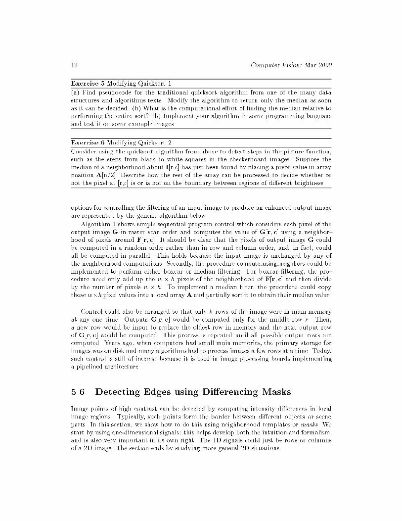
Exercise 5 Modifying Quicksort 1
(a) Find pseudocode for the traditional quicksort algorithm from one of the many data
structures and algorithms texts. Modify the algorithm to return only the median as soon
as it can be decided. (b) What is the computational e�ort of �nding the median relative to
performing the entire sort? (b) Implement your algorithm in some programming language
and test it on some example images.
Exercise 6 Modifying Quicksort 2
Consider using the quicksort algorithm from above to detect steps in the picture function,
such as the steps from black to white squares in the checkerboard images. Suppose the
median of a neighborhood about I[r,c] has just been found by placing a pivot value in array
position A[n/2]. Describe how the rest of the array can be processed to decide whether or
not the pixel at [r,c] is or is not on the boundary between regions of di�erent brightness.
options for controlling the �ltering of an input image to produce an enhanced output image
are represented by the generic algorithm below.
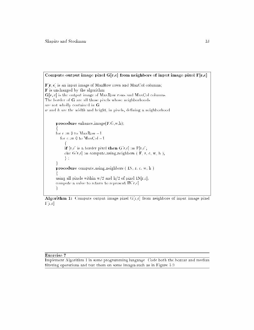
Algorithm 1 shows simple sequential program control which considers each pixel of the
output image G in raster scan order and computes the value of G[r; c] using a neighbor-
hood of pixels around F[r; c]. It should be clear that the pixels of output image G could
be computed in a random order rather than in row and column order, and, in fact, could
all be computed in parallel. This holds because the input image is unchanged by any of
the neighborhood computations. Secondly, the procedure compute using neighbors could be
implemented to perform either boxcar or median �ltering. For boxcar �ltering, the pro-
cedure need only add up the w � h pixels of the neighborhood of F[r; c] and then divide
by the number of pixels w � h. To implement a median �lter, the procedure could copy
those w�h pixel values into a local arrayA and partially sort it to obtain their median value.
Control could also be arranged so that only h rows of the image were in main memory
at any one time. Outputs G[r; c] would be computed only for the middle row r. Then,
a new row would be input to replace the oldest row in memory and the next output row
of G[r; c] would be computed. This process is repeated until all possible output rows are
computed. Years ago, when computers had small main memories, the primary storage for
images was on disk and many algorithms had to process images a few rows at a time. Today,
such control is still of interest because it is used in image processing boards implementing
a pipelined architecture.
5.6 Detecting Edges using Di�erencing Masks
Image points of high contrast can be detected by computing intensity di�erences in local
image regions. Typically, such points form the border between di�erent objects or scene
parts. In this section, we show how to do this using neighborhood templates or masks. We
start by using one-dimensional signals: this helps develop both the intuition and formalism,
and is also very important in its own right. The 1D signals could just be rows or columns
of a 2D image. The section ends by studying more general 2D situations.
Shapiro and Stockman 13
Compute output image pixel G[r,c] from neighbors of input image pixel F[r,c].
F[r; c] is an input image of MaxRow rows and MaxCol columns;
F is unchanged by the algorithm.
G[r; c] is the output image of MaxRow rows and MaxCol columns.
The border of G are all those pixels whose neighborhoods
are not wholly contained in G.
w and h are the width and height, in pixels, de�ning a neighborhood.
procedure enhance image(F,G,w,h);
ffor r := 0 to MaxRow - 1
for c := 0 to MaxCol - 1
fif [r,c] is a border pixel then G[r,c] := F[r,c];
else G[r,c] := compute using neighbors ( F, r, c, w, h );
g ;gprocedure compute using neighbors ( IN, r, c, w, h )
fusing all pixels within w/2 and h/2 of pixel IN[r,c],
compute a value to return to represent IN[r,c]
g
Algorithm 1: Compute output image pixel G[r,c] from neighbors of input image pixel
F[r,c].
Exercise 7Implement Algorithm 1 in some programming language. Code both the boxcar and median
�ltering operations and test them on some images such as in Figure 5.9.

14 Computer Vision: Mar 2000
5.6.1 Di�erencing 1D Signals
S =
S’ =
S" =
M’ =
M" = +1 - 2
-1 +1
+1
f ( x )
oo
oo
S [ i ] S[ i+1 ] S [ i+2 ]S[ i-1 ]
S [ i ]- S[i-1]
S [ i+1 ]- S [ i ]
S [ i+1 ] - 2 S [ i ] + S [ i-1 ]
Figure 5.10: (Left) The �rst (S') and second (S") di�erence signals are scaled approxima-
tions to the �rst and second derivatives of the signal S. (Right) MasksM' andM" represent
the derivative operations.
Figure 5.10 shows how masks can be used to compute representations of the derivatives
of a signal. Given that the signal S is a sequence of samples from some function f , then
f 0(xi) � (f(xi) � f(xi�1)=(xi � xi�1). Assuming that the sample spacing is �x = 1, the
derivative of f(x) can be approximated by applying the mask M0 = [�1;1] to the sam-
ples in S as shown in Figure 5.10 to obtain an output signal S'. As the �gure shows, it's
convenient to think of the values of S' as occurring in between the samples of S. A high
absolute value of S'[i] indicates where the signal is undergoing rapid change or high contrast.Signal S' itself can be di�erentiated a second time using mask M0 to produce output S"
which corresponds to the second derivative of the original function f . The important result
illustrated in Figure 5.10 and derived in the equations below is that the approximate second
derivative can be computed by applying the maskM00 to the original sequence of samples S.
S0[i] = �S[i � 1] + S[i] (5.3)
mask M0 = [�1; +1] (5.4)
S00[i] = �S0[i] + S0[i+ 1] (5.5)
= �(S[i]� S[i � 1]) + (S[i + 1]� S[i]) (5.6)
= S[i � 1]� 2S[i] + S[i + 1] (5.7)

Shapiro and Stockman 15
mask M00 = [1; �2; 1] (5.8)
mask M = [�1;0;1]
S1 12 12 12 12 12 24 24 24 24 24
S1 M 0 0 0 0 12 12 0 0 0 0
(a) S1 is an upward step edge
S2 24 24 24 24 24 12 12 12 12 12
S2 M 0 0 0 0 -12 -12 0 0 0 0
(b) S2 is a downward step edge
S3 12 12 12 12 15 18 21 24 24 24
S3 M 0 0 0 3 6 6 6 3 0 0
(c) S3 is an upward ramp
S4 12 12 12 12 24 12 12 12 12 12
S4 M 0 0 0 12 0 -12 0 0 0 0
(d) S4 is a bright impulse or \line"
Figure 5.11: Cross correlation of four special signals with �rst derivative edge detecting
mask [�1; 0; 1]; (a) upward step edge, (b) downward step edge, (c) upward ramp, and (d)
bright impulse. Note that, since the coordinates of M sum to zero, output must be zero on
a constant region.
If only points of high contrast are to be detected, it is very common to use the absolute
value after applying the mask at signal position S[i]. If this is done, then the �rst derivative
mask can be either M0 = [�1;+1] or [+1;�1] and the second derivative mask can be either
M00 = [+1;�2;+1] or [�1;+2;�1]. A similar situation exists for 2D images as we shall
soon see. Whenever only magnitudes are of concern, we will consider these patterns to be
the same, and whenever the sign of the change is important, we will consider them to be
di�erent.
Use of another common�rst derivative mask is shown in Figure 5.11. This mask has 3 co-
ordinates and is centered at signal point S[i] so that it computes the signal di�erence across
the adjacent values. Because �x = 2, it will give a high estimate of the actual derivative
unless the result is divided by 2. Moreover, this mask is known to give a response on perfect
step edges that is 2 samples wide, as is shown in Figure 5.11(a)-(b). Figure 5.12 shows the
response of the second derivative mask on the sample signals. As Figure 5.12 shows, signal
contrast is detected by a zero-crossing, which localizes and ampli�es the change between two
successive signal values. Taken together, the �rst and second derivative signals reveal much
of the local signal structure. Figure 5.13 shows how smoothing of signals can be put into
16 Computer Vision: Mar 2000
the same framework as di�erencing: the boxed table below compares the general properties
of smoothing versus di�erencing masks.
Some properties of derivative masks follow:
� Coordinates of derivative masks have opposite signs in order to obtain a high response
in signal regions of high contrast.
� The sum of coordinates of derivative masks is zero so that a zero response is obtained
on constant regions.
� First derivative masks produce high absolute values at points of high contrast.
� Second derviatve masks produce zero-crossings at points of high contrast.
For comparison, smoothing masks have these properties:
� Coordinates of smoothing masks are positive and sum to one so that output on con-
stant regions is the same as the input.
� The amount of smoothing and noise reduction is proportional to the mask size.
� Step edges are blurred in proportion to the mask size.
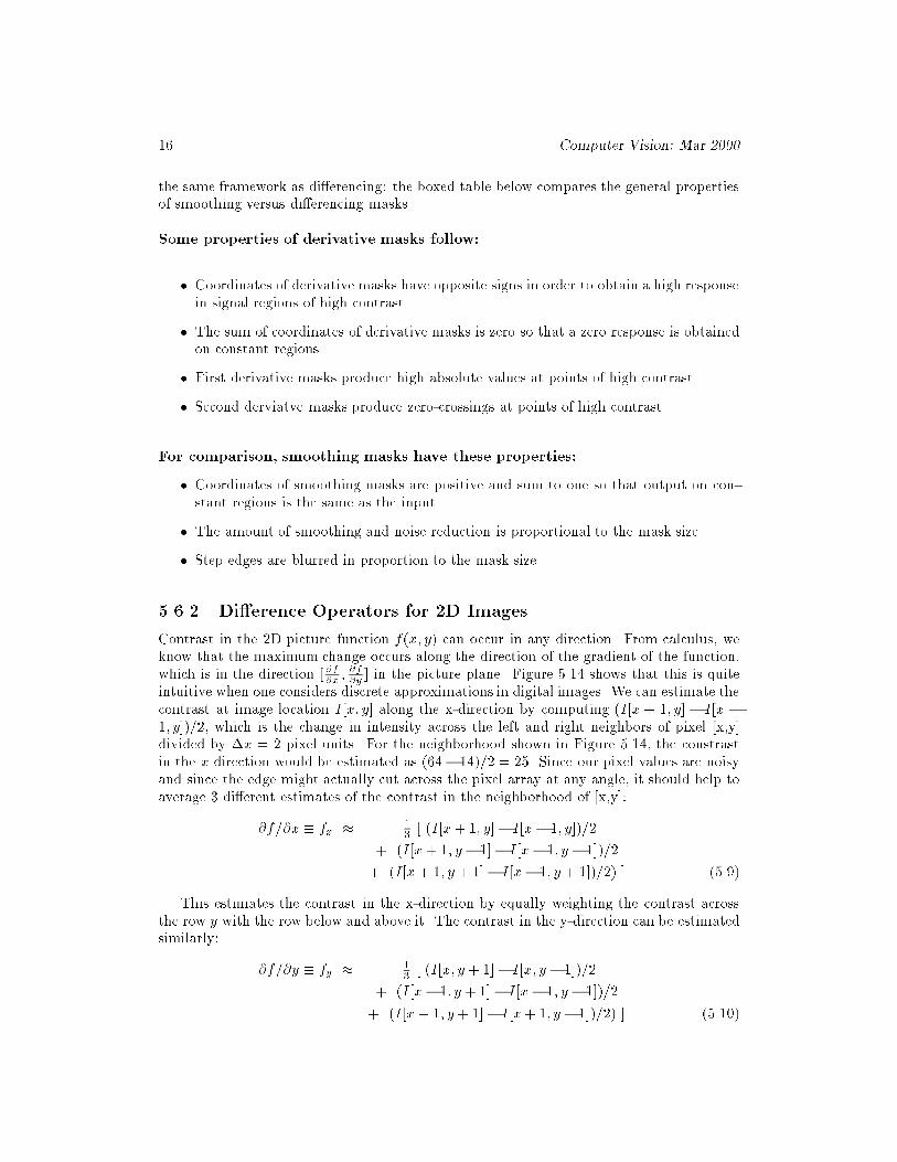
5.6.2 Di�erence Operators for 2D Images
Contrast in the 2D picture function f(x; y) can occur in any direction. From calculus, we
know that the maximum change occurs along the direction of the gradient of the function,
which is in the direction [@f@x; @f@y] in the picture plane. Figure 5.14 shows that this is quite
intuitive when one considers discrete approximations in digital images. We can estimate the
contrast at image location I[x; y] along the x-direction by computing (I[x + 1; y] � I[x �1; y])=2, which is the change in intensity across the left and right neighbors of pixel [x,y]
divided by �x = 2 pixel units. For the neighborhood shown in Figure 5.14, the constrast
in the x direction would be estimated as (64� 14)=2 = 25. Since our pixel values are noisy
and since the edge might actually cut across the pixel array at any angle, it should help to
average 3 di�erent estimates of the contrast in the neighborhood of [x,y]:
@f=@x � fx � 13[ (I[x+ 1; y]� I[x� 1; y])=2
+ (I[x+ 1; y � 1]� I[x� 1; y � 1])=2
+ (I[x + 1; y + 1]� I[x� 1; y + 1])=2) ] (5.9)
This estimates the contrast in the x-direction by equally weighting the contrast across
the row y with the row below and above it. The contrast in the y-direction can be estimated
similarly:
@f=@y � fy � 13[ (I[x; y + 1]� I[x; y � 1])=2
+ (I[x� 1; y + 1]� I[x� 1; y � 1])=2
+ (I[x+ 1; y + 1]� I[x+ 1; y � 1])=2) ] (5.10)

Shapiro and Stockman 17
mask M = [�1;2;�1]
S1 12 12 12 12 12 24 24 24 24 24
S1 M 0 0 0 0 -12 12 0 0 0 0
(a) S1 is an upward step edge
S2 24 24 24 24 24 12 12 12 12 12
S2 M 0 0 0 0 12 -12 0 0 0 0
(b) S2 is a downward step edge
S3 12 12 12 12 15 18 21 24 24 24
S3 M 0 0 0 -3 0 0 0 3 0 0
(c) S3 is an upward ramp
S4 12 12 12 12 24 12 12 12 12 12
S4 M 0 0 0 -12 24 -12 0 0 0 0
(d) S4 is a bright impulse or \line"
Figure 5.12: Cross correlation of four special signals with second derivative edge detecting
mask M = [�1;2;�1]; (a) upward step edge, (b) downward step edge, (c) upward ramp,
and (d) bright impulse. Since the coordinates of M sum to zero, response on constant
regions is zero. Note how a zero-crossing appears at an output position where di�erent
trends in the input signal join.

18 Computer Vision: Mar 2000
box smoothing mask M = [1=3;1=3;1=3]
S1 12 12 12 12 12 24 24 24 24 24
S1 M 12 12 12 12 16 20 24 24 24 24
(a) S1 is an upward step edge
S4 12 12 12 12 24 12 12 12 12 12
S4 M 12 12 12 16 16 16 12 12 12 12
(d) S4 is a bright impulse or \line"
Gaussian smoothing mask M = [1=4;1=2;1=4]
S1 12 12 12 12 12 24 24 24 24 24
S1 M 12 12 12 12 15 21 24 24 24 24
(a) S1 is an upward step edge
S4 12 12 12 12 24 12 12 12 12 12
S4 M 12 12 12 15 18 15 12 12 12 12
(d) S4 is a bright impulse or \line"
Figure 5.13: (Top two rows) Smoothing of step and impulse with box mask [1=3; 1=3; 1=3];
(bottom two rows) smoothing of step and impulse with Gaussian mask [1=4; 1=2; 1=4].

Shapiro and Stockman 19
y-1
y+1 38
14
12 15 42
65
64
66
35
f y
θ
x-1 x+1
y
x
y
f
2
θ -1
= 42 degrees
f = ( (38-12)/2 + (66-15)/2 + (65-42)/2 ) / 3
1/22
= tan (16 / 18) = 0.727 rad
| f | = ( 16 + 18 ) = 24
f = ( (65-38)/2 + (64-14)/2 + (42-12)/2 ) / 3
x
lowerintensities
higher intensities= ( 13 + 25 + 11 ) / 3 = 16
= ( 13 + 25 + 15 ) / 3 = 18
f x
Figure 5.14: Estimating the magnitude and direction of contrast at I[x,y] by estimating the
gradient magnitude and direction of picture function f(x; y) using the discrete samples in
the image array.
Often, the division by 6 is ignored to save computation time, resulting in scaled estimates.
Masks for these two contrast operators are denoted byMx and My at the top of Figure 5.15.
The gradient of the picture function can be estimated by applying the masks to the 8-
neighborhood N8[x; y] of pixel [x; y] as given in Equations 5.11 to 5.14. These masks de�ne
the Prewitt operator credited to Dr Judith Prewitt who used them in detecting boundaries
in biomedical images.
@f
@x� (1=6)(Mx �N8[x; y]) (5.11)
@f
@y� (1=6)(My �N8[x; y]) (5.12)
j rf j �
s@f
@x
2
+@f
@y
2
(5.13)
� � tan�1(@f
@y=@f
@x) (5.14)
The operation M � N is de�ned formally in the next section: operationally, mask M is
overlaid on image neighborhood N so that each intensity Nij can be multiplied by weight
Mij ; �nally all these products are summed. The middle row of Figure 5.15 shows the two
analogous Sobel masks; their derivation and interpretation is the same as for the Prewitt
masks except that the assumption is that the center estimate should be weighted twice as
much as the estimate to either side.
The Roberts masks are only 2x2; hence they are both more e�cient to use and more lo-
cally applied. Often referred to as the Roberts cross operator, these masks actually compute
a gradient estimate at the center of a 4-neighborhood and not at a center pixel. More-
over, the actual coordinate system in which the operator is de�ned is rotated 45� o� the
standard row direction. Application of the Roberts cross operator is shown in Figure 5.16:

20 Computer Vision: Mar 2000
Prewitt: Mx =
-1 0 1
-1 0 1
-1 0 1
; My =
1 1 1
0 0 0
-1 -1 -1
Sobel: Mx =
-1 0 1
-2 0 2
-1 0 1
; My =
1 2 1
0 0 0
-1 -2 -1
Roberts: Mx =0 1
-1 0; My =
1 0
0 -1
Figure 5.15: 3x3 masks used to estimate the gradient of picture function f(x; y): (top row)
Prewitt; (middle row) Sobel; (bottom row) Roberts.
the original input image is shown in the upper left, while the highest 10% of the responses
of the operator are shown at the lower left. Qualitatively, these results are typical of the
several small-neighborhood operators { many pixels on many edges are detected but some
gaps exist. Also, there are strong responses on the highly textured regions corresponding
to plants. The Roberts results should be compared to the results obtained by combining
the simple 1D row and column masks shown in Figure 5.16(b-d) and (f-h). It is common
to avoid computing a square root in order to compute gradient magnitude; alternatives are
max( j @f@xj ; j @f
@yj ), j @f
@xj + j @f
@yj , or (@f
@x
2+ @f
@y
2)=2. With these estimates, one must
be careful when trying to interpret the actual gradient or gradient direction. Figure 5.17(b)
shows the results of using the Sobel 3x3 operator to compute mean square gradient mag-
nitude and Figure 5.17(c) shows an encoding of the gradient direction. The small squares
in the original image are 8x8 pixels: the Sobel operator represents many, but not all, of the
image edges.
Exercise 8
If a true gradient magnitude is needed, why might the Sobel masks provide a faster solution
than the Prewitt masks?
Exercise 9 *Optimality of Prewitt masks
The problem is to prove that Prewitt masks give the weights for the best �tting plane
approximating the intensity surface in a 3 � 3 neighborhood, assuming all 9 samples have
equal weight. Suppose that the 9 intensities I[r + i; c + j]; i; j = �1; 0; 1 of a 3 � 3 image
neighborhood are �t by the least squares planar model I[r; c] = z = pr+ qc+ z0. (Recall
that the 9 samples are equally spaced in terms of r and c.) Show that the Prewitt masks
compute the estimates of p and q as the partial derivatives of the least squares planar �t of
the intensity function.
Figure 5.18 (top) shows plots of the intensites of two rows of the room scene at the
left. The lower row cuts across four dark regions as seen in the image and the plot; (1)
the coat on the chair at the left (columns 20 to 80), (2) Dr Prewitt's chair and dress in the

Shapiro and Stockman 21
(a) (b) (c) (d)
(e) (f) (g) (h)
Figure 5.16: (a) Original house image; (b) top 5% of the responses from horizontal edge
mask [+1;�1] t; (c) top 5% of the responses from horizontal edge mask [�1;+1] t; (d)
images of (b) and (c) ORed together; (e) top 10% of the sum of the absolute values of
the two Roberts mask responses; (f) top 5% of the responses from the vertical edge mask
[�1;+1]; (g) top 5% of the responses from the vertical edge mask [+1;�1]; (h) images (f)
and (g) ORed together.
center (columns 170 to 240), (3) the shadow of the rightmost chair (columns 360 to 370)
and (4) the electric wires (column 430). Note that the transitions between dark and bright
are sharp except for the boundary between the chair and its shadow, which ramps down
from brightness 220 to 20 over about 10 pixels. The upper row pro�le, shown at the top
right, shows sharp transitions where it cuts across the picture frames, mat, and pictures.
The picture at the left shows much more intensity variation than the one at the right. The
bottom row of Figure 5.18 shows the results of applying the 3x3 Prewitt gradient operator
to the original image. The sum of the absolute values of the column and row gradients
fx and fy is plotted for the same two image rows shown at the top of the �gure. The
highest values of the Prewitt operator correspond well with the major boundaries crossed;
however, the several medium level spikes from Dr Prewitt's chair between columns 170
and 210 are harder to interpret. The contrasts in the upper row, graphed at the bottom
right, are interpeted similarly { major object boundaries correspond well to the object
boundaries of the picture frame and mat; however, there is a lot of intensity variation in
the leftmost picture. Generally, gradient operators work well for detecting the boundary
of isolated objects, although some problems are common. Boundaries sometimes drop out
due to object curvature or soft shadows: on the other hand, good contrast often produces
boundaries that are several pixels wide, necessitating a thinning step afterward. Gradient
operators will also respond to textured regions, as we shall study in more detail in Chapter
7.

22 Computer Vision: Mar 2000
(a) (b) (c)
Figure 5.17: (a) Image of noisy squares and rings; (b) mean square response of 3x3 Sobel
operator; (c) coding of gradient direction computed by 3x3 Sobel operator.
0
50
100
150
200
250
0 50 100 150 200 250 300 350 400 450
’prewittR250’
0
50
100
150
200
250
0 50 100 150 200 250 300 350 400 450
’prewittR20’
(a) (b) (c)
0
50
100
150
200
250
300
0 50 100 150 200 250 300 350 400 450
’prewittF7I250’
0
50
100
150
200
250
300
0 50 100 150 200 250 300 350 400 450
’prewittF7I20’
(d) (e) (f)
Figure 5.18: (a) Image of Judith Prewitt with two rows selected; (b) plot of intensities along
selected lower row; (c) plot of intensities along selected upper row; (d) \gradient image"
showing result of j fx j + j fy j using the Prewitt 3x3 operator; (e) plot of selected lower
row of gradient image; (f) plot of selected upper row of gradient image.

Shapiro and Stockman 23
5.7 Gaussian Filtering and LOG Edge Detection
The Gaussian function has important applications in many areas of mathematics, including
image �ltering. In this section, we highlight the characteristics that make it useful for
smoothing images or detecting edges after smoothing.
8 Definition AGaussian function of one variable with spread � is of the following form,where c is some scale factor.
g(x) = ce�x2
2�2 (5.15)
A Gaussian function of two variables is
g(x; y) = ce�(x2+y2)
2�2 (5.16)
These forms have the same structure as the normal distribution de�ned in Chapter 4,
where the constant c was set so that the area under the curve would be 1. To create a mask
for �ltering, we usually make c a large number so that all mask elements are integers. The
Gaussian is de�ned centered on the origin and thus needs no location parameter � as does
the normal distribution: an image processing algorithm will translate it to wherever it will
be applied in a signal or image. Figure 5.19 plots the Gaussian of one variable along with its
�rst and second derivatives, which are also important in �ltering operations. The derivation
of these functions is given in Equations 5.17 to 5.22. The area under the function g(x) is 1,
meaning that it is immediately suitable as a smoothing �lter that does not a�ect constant
regions. g(x) is a positive even function; g0(x) is just g(x) multiplied by odd function �xand scaled down by �2. More structure is revealed in g00(x). Equation 5.21 shows that g00(x)is the di�erence of two even functions and that the central lobe will be negative with x � 0.
Using Equation 5.22, it is clear that the zero crossings of the second derviative occur at
x = ��, in agreement with the plots in Figure 5.19.
g(x) =1p2� �
e�x2
2�2 (5.17)
g0(x) =�1p2� �3
xe�x2
2�2 (5.18)
=�x�2
g(x) (5.19)
g00(x) = (x2p2� �5
� 1p2� �3
) e�x2
2�2 (5.20)
=x2
�4g(x) � 1
�2g(x) (5.21)
= (x2
�4� 1
�2) g(x) (5.22)
Understanding the properties of the 1D Gaussian, we can now intuitively create the corre-
sponding 2D function g(x; y) and its derivatives by making the substitution r =px2 + y2.
This creates the 2D forms by just spinning the 1D form about the vertical axis yielding
isotropic functions which have the same 1D Gaussian cross section in any cut through the
origin. The second derivative form is well known as a sombrero or Mexican hat. From

24 Computer Vision: Mar 2000
-0.1
-0.05
0
0.05
0.1
0.15
0.2
0.25
0.3
-10 -5 0 5 10
Gaussian g(x) with mean 0 and standard deviation 2
g(x)
-0.1
-0.05
0
0.05
0.1
-10 -5 0 5 10
First derivative of Gaussian with mean 0 and standard deviation 2
g1(x)
(a) (b)
-0.1
-0.05
0
0.05
0.1
-10 -5 0 5 10
2nd derivative of Gaussian with mean 0 and standard deviation 2
g2(x)
-0.1
-0.05
0
0.05
0.1
0.15
0.2
0.25
-10 -5 0 5 10
Gaussian g(x): sigma=2, and 1st and 2nd derivatives
g(x)g1(x)g2(x)
(c) (d)
Figure 5.19: (a) Gaussian g(x) with spread � = 2; (b) �rst derivative g0(x); (c) secondderivative g00(x), which looks like the cross section of a sombrero upside down from how it
would be worn; (d) all three plots superimposed to show how the extreme slopes of g(x)
align with the extremas of g0(x) and the zero crossings of g00(x).
the mathematical derivations, the cavity for the head will be pointed upward along the
z = g(x; y) axis; however, it is usually displayed and used in �ltering with the cavity pointed
downward, or equivalently, with the center lobe positive and the rim negative.

Shapiro and Stockman 25
G3�3 =1 2 1
2 4 2
1 2 1
; G7�7 =
1 3 7 9 7 3 1
3 12 26 33 26 12 3
7 26 55 70 55 26 7
9 33 70 90 70 33 9
7 26 55 70 55 26 7
3 12 26 33 26 12 3
1 3 7 9 7 3 1
Figure 5.20: (Left) A 3�3 mask approximatinga Gaussian obtained by matrixmultiplication
[1; 2; 1]t [1; 2; 1]; (Right) a 7� 7 mask approximating a Gaussian with �2 = 2 obtained by
using Equation 5.16 to generate function values for integers x and y and then setting c = 90
so that the smallest mask element is 1.
Some Useful Properties of Gaussians
1. Weight decreases smoothly to zero with distance from the origin, meaning
that image values nearer the central location are more important than values
that are more remote; moreover, the spread parameter � determines how
broad or focused the neighborhood will be. 95% of the total weight will be
contained within 2� of the center.
2. Symmetry about the abscissa; ipping the function for convolution produces
the same kernel.
3. Fourier transformation into the frequency domain produces another Gaus-
sian form, which means convolution with a Gaussian mask in the spatial
domain reduces high frequency image trends smoothly as spatial frequency
increases.
4. The second derivative of a 1D Gaussian g00(x) has a smooth center lobe of
negative area and two smooth side lobes of positive area: the zero crossings
are located at �� and +�, corresponding to the in ection points of g(x) and
the extreme points of g0(x).
5. A second derivative �lter based on the Laplacian of the Gaussian is called
a LOG �lter. A LOG �lter can be approximated nicely by taking the
di�erence of two Gaussians g00(x) � c1e� x2
2�12 � c2e
� x2
2�22 , which is often
called a DOG �lter (for Di�erence Of Gaussians). For a positive center
lobe, we must have �1 < �2; also, �2 must be carefully related to �1 to
obtain the correct location of zero crossings and so that the total negative
weight balances the total positive weight.
6. The LOG �lter responds well to intensity di�erences of two kinds { small
blobs coinciding with the center lobe, and large step edges very close to the
center lobe.
Two di�erent masks for Gaussian smoothing are shown in Figure 5.20. Masks for edge
detection are given below.

26 Computer Vision: Mar 2000
-0.1
-0.05
0
0.05
0.1
-10 -5 0 5 10
Sombrero: Gaussian -g(x): sigma=2
-1*g2(x)
0 -1 0
-1 4 -1
0 -1 0
5 5 5 5 5 5
5 5 5 5 5 5
5 5 10 10 10 10
5 5 10 10 10 10
5 5 5 10 10 10
5 5 5 5 10 10
- - - - - -
- 0 -5 -5 -5 -
- -5 10 5 5 -
- -5 10 0 0 -
- 0 -10 10 0 -
- - - - - -
Figure 5.21: (Top row) Cross section of the LOG �lter and a 3� 3 mask approximating it;
(bottom row) input image and result of applying the mask to it.
5.7.1 Detecting Edges with the LOG Filter
Two di�erent masks implementating the LOG �lter are given in Figures 5.21 and 5.22. The
�rst is 3 � 3 mask: the smallest possible implementation, detects image details nearly the
size of a pixel. The 11�11 mask computes a response by integrating the input of 121 pixels
and thus responds to larger image features and not smaller ones. Integrating 121 pixels can
take a lot more time than integrating 9 of them done in software.
Exercise 10 Properties of the LOG �lter
Suppose that the 9 intensities of a 3� 3 image neighborhood are perfectly �t by the planar
model I[r; c] = z = pr + qc+ z0. (Recall that the 9 samples are equally spaced in terms
of r and c.) Show that the simple LOG mask
0 -1 0
-1 4 -1
0 -1 0
has zero response on such a
neighborhood. This means that the LOG �lter has zero response on both constant regions
and ramps.
5.7.2 On Human Edge-Detection
We now describe an arti�cial neural network (ANN) architecture which implements the LOG
�ltering operation in a highly parallel manner. The behavior of this network has been shown

Shapiro and Stockman 27
0 0 0 -1 -1 -2 -1 -1 0 0 0
0 0 -2 -4 -8 -9 -8 -4 -2 0 0
0 -2 -7 -15 -22 -23 -22 15 -7 -2 0
-1 -4 -15 -24 -14 -1 -14 -24 -15 -4 -1
-1 -8 -22 -14 52 103 52 -14 -22 -8 -1
-2 -9 -23 -1 103 178 103 -1 -23 -9 -2
-1 -8 -22 -14 52 103 52 -14 -22 -8 -1
-1 -4 -15 -24 -14 -1 -14 -24 -15 -4 -1
0 -2 -7 -15 -22 -23 -22 15 -7 -2 0
0 0 -2 -4 -8 -9 -8 -4 -2 0 0
0 0 0 -1 -1 -2 -1 -1 0 0 0
Figure 5.22: An 11 � 11 mask approximating the Laplacian of a Gaussian with �2 = 2.
(From Harlalick and Shapiro, Volume I, page 349.)
-1 +2 -1
b ca
-a +2b -c = out
intensity 20
intensity 30
0 0 0 -10 +10 0 0 0
level 1
level 2
g
g
gg
intensity 0 intensity 0
difference is now 20
Figure 5.23: Producing the Mach band e�ect using an ANN architecture. Intensity is sensed
by cells of the retina (level 1) which then stimulate integrating cells in a higher level layer
(level 2).
Figure 5.24: Seven constant stripes generated with grey levels 31 + 32k; k = 1; 7. Due to
the Mach band e�ect, humans perceive scalloped, or concave, panels.

28 Computer Vision: Mar 2000
-+
-
-
-+++
+ -
retinal level
B
a
ef
dc
A
integrating level
receptive field for neuron BA
neuronforfieldreceptive
intensity edge-
- -
- -
- -
--b++
+
++
+ +
Figure 5.25: A 3D ANN architecture for LOG �ltering.
to simulate some of the known behaviors of the human visual system. Moreover, invasive
techniques have also shown that the visual systems of cats and monkeys produce electrical
signals consistent with the behavior of the neural network architecture. Figure 5.23 shows
the processing of 1D signals. A step edge is sensed at various points by cells of the retinal
array. These level 1 cells stimulate the integrating cells at level 2. Each physical connection
between level 1 cell i and level 2 cell j has an associated weight wij which is multiplied
by the stimulus being communicated before it is summed in cell j. The output of cell j is
yj =PN
i=1wijxi where xi is the output of the i-th �rst level cell and N is the total number
of �rst level cells. (Actually, we need only account for those cells i directly connected to the
second level cell j). By having the weights associated with each connection, it is possible,
and common, to have the same cell i give positive input to cell j and negative input to
cell k 6= j. Figure 5.23 shows that each cell j of the second level computes its output as
�a + 2b � c, corresponding to the mask [�1; 2;�1]: the weight 2 is applied to the central
input, while the (inhibitory) inputs a and b are each weighted by -1.
This kind of architecture can be de�ned for any kind of mask and permits a highly par-
allel implementation of cross correlation for �ltering or feature detection. The psychologist
Mach noted that humans perceive an edge between two regions as if it were pulled apart
to exaggerate the intensity di�erence, as is done in Figure 5.23. Note that this architecture
and mask create the zero crossing at the location of the edge between two cells, one of which
produces positive output and the other negative output. The Mach band e�ect changes the
perceived shape of joining surfaces and is evident in computer graphics systems that display
polyhedral objects via shaded faces. Figure 5.24 shows seven constant regions, stepping
from grey level 31 to 255 in steps of 32. Do you perceive concave panels in 3D such as on a
Doric column from a Greek temple?
Figure 5.25 extends Figure 5.23 to 2D images. Each set of retinal cells connected to
integrating cell j comprise what is called the receptive �eld of that cell. To perform edge
detection via a second derivative operation, each receptive �eld has a center set of cells

Shapiro and Stockman 29
which have positive weights wij with respect to cell j and a surrounding set of cells with
negative weights. Retinal cells b and c are in the center of the receptive �eld of integrat-
ing cell A, whereas retinal cells a and d are in the surround and provide inhibitory input.
Retinal cell d is in the center of the receptive �eld of integrating cell B, however, and cell
c is in its surround. The sum of the weights from the center and the surround should be
zero so that the integrating cell has neutral output on constant regions. Because the center
and surround are circular, output will not be neutral whenever a straight region boundary
just nips the center area, regardless of the angle. Thus, each integrating cell is an isotropicedge detector cell. Additionally, if a small region contrasting with the background images
within the center of the receptive �eld the integrating cell will also respond, making it a spot
detector as well. Figure 5.21 shows the result of convolving the smallest of the LOG masks
with an image containing two regions. The result at the right of the �gure shows how the
operation determines the boundary between the regions via zero crossings. An 11�11 mask
corresponding to the Laplacian of a Gaussian with �2 = 2 is shown in Figure 5.22. The
tiny mask is capable of �nding the boundary between tiny regions and is sensitive to high
curvature bouundaries but will also respond to noise texture. The larger mask performs a
lot of smoothing and will only respond to boundaries between larger regions with smoother
perimeter.
Exercise 11Give more detailed support to the above arguments that the integrating cells shown in
Figure 5.25 (a) respond to contrasting spots or blobs that image within the center of the
�eld and (b) respond to boundaries between two large regions that just barely cross into
the center of the �eld.
5.7.3 Marr-Hildreth Theory
David Marr and Ellen Hildreth proposed LOG �ltering to explain much of the low level
behavior of human vision. Marr proposed that the objective of low level human visual
processing was the construction of a primal sketch which was a 2D description containing
lines, edges, and blobs. (The primal sketches derived from the two eyes would then be
processed further to derive 3D interpretations of the scene.) To derive a primal sketch, Marr
and Hildreth proposed an organization based on LOG �ltering with 4 or 5 di�erent spreads
�. The mathematical properties outlined above explained the results of both perceptual
experiments on humans and invasive experiments with animals. LOG �lters with large �
would detect broad edges while those with small � would focus on small detail. Coordination
of the output from the di�erent scales could be done at a higher level, perhaps with the large
scale detections guiding those at the small scale. Subsequent work has produced di�erent
practical scale space methods of integrating output from detectors of di�erent sizes.
Figure 5.26 shows an image processed at two di�erent levels of Gaussian smoothing. The
center image shows good representation of major objects and edges, whereas the rightmost
image shows both more image detail and more noise. Note that the ship and part of the
sand/water boundary is represented in the rightmost image but not in the center image.
Marr's primal sketch also contained descriptions of virtual lines, which are formed by similar
detected features organized along an image curve. These might be the images of a dotted
line, a row of shrubs, etc. A synthetic image containing a virtual line is shown in Figure 5.27

30 Computer Vision: Mar 2000
original smoothed � = 4 smoothed � = 1
Figure 5.26: An input image (a) is smoothed using Gaussian �lters of size (b) � = 4 and
(c) � = 1 before performing edge detection. More detail and more noise is shown for the
smaller �lter (photo by David Sha�er 1998).
Figure 5.27: (Left) A virtual line formed by the termination points of a line texture {
perhaps this is two pieces of wrapping paper overlaid; (center) output from a speci�c 4� 4
LOG �lter responds to both lines and endpoints; (right) a di�erent 3�3 LOG �lter responds
only to the endpoints.
along with the output of two di�erent LOG �lters. Both LOG �lters give a response to the
ends of the stripes; one is sensitive to the edges of the stripes as well, but the other is
not. Figure 5.28 shows the same principle in a real image that was thresholded to obtain
an artistic texture. Recent progress in researching the human visual system and brain has
been rapid: results seem to complicate the interpretations of earlier work on which Marr
and Hildreth based their mathematical theory. Nevertheless, use of variable-sized Gaussian
and LOG �lters is �rmly established in computer vision.
5.8 The Canny Edge Detector
The Canny edge detector is a very popular and e�ective operator, and it is important to
introduce it here, although details are placed in Chapter 10. The Canny operator �rst
smoothes the intensity image and then produces extended contour segments by following
high gradient magnitudes from one neighborhood to another. Figure 5.29 shows edge de-
tection in fairly di�cult outdoor images. The contours of the arch of St. Louis are detected

Shapiro and Stockman 31
Figure 5.28: Picture obtained by thresholding: object boundaries are formed by virtual
curves formed by the ends of stripes denoting cross sections of generalized cylinders. (Orig-
inal photo by Eleanor Harding.
quite well in Figure 5.29: using a parameter of � = 1 detects some of the metal seams of
the arch as well as some internal variations in the tree, whereas use of � = 4 detects only
the exterior boundaries of these objects. As shown in the bottom row of Figure 5.29, the
operator isolates many of the texture elements of the checkered ags. For comparison, use
of the Roberts operator with a low threshold on gradient magnitude is shown: more texture
elements of the scene (grass and fence) are evident, although they have less structure than
those in the Canny output. The algorithm for producing contour segments is treated in
detail in Chapter 10.
5.9 *Masks as Matched Filters
Here we give a theoretical basis for the concept that the response of a mask to a certain
image neighborhood is proportional to how similar that neighborhood is to the mask. The
important practical result of this is that we now know how to design masks to detect speci�c
features { we just design a mask that is similar to the feature[s] we want to detect. This will
serve us well in both edge and texture detection and also in detecting other special patterns
such as holes or corners. We introduce the concepts using 1-dimensional signals, which are
important in their own right, and which might correspond to rows or columns or any other
cut through a 2D image. The concepts and mathematical theory immediately extend to the
2D case.
5.9.1 The Vector Space of all Signals of n Samples
For a given n � 1, the set of all vectors of n real coordinates forms a vector space. The
practical and powerful vector space operations which we use are summarized below. The
reader has probably already worked with vectors with n = 2 or n = 3 when studying

32 Computer Vision: Mar 2000
Figure 5.29: (Top left) Image of the great arch at St Louis; (top center) results of Canny
operator with � = 1; ( top right) results of Canny operator with � = 4; (bottom left) image
with textures; (bottom center) results of Canny operator with � = 1; (bottom right) results
of Roberts operator thresholded to pass the top 20% of the pixels in gradient magnitude.
analytical geometry or calculus. For n = 2 or n = 3, the notion of vector length is the same
as that used in plane geometry and 3D analytical geometry since Euclid. In the domain of
signals, length is related to energy of the signal, de�ned as the squared length of the signal,
or equivalently, just the sum of the squares of all coordinates. Signal energy is an extremely
useful concept as will be seen.
9 Definition The energy of signal S = [s1; s2; :::; sn] is k S k2 = s12 + s2
2 + : : :+ sn2.
Note that in many applications, the full range of real-valued signals do not arise because
negative values are impossible for the coordinates. For example, a 12-dimensional vector
recording the rainfall at a particular location for each of the 12 months should have no
negative coordinates. Similarly, intensities along an image row are commonly kept in a
non-negative integer range. Nevertheless, the vector space interpretation is still useful, as
we shall see. Often, the mean signal value is subtracted from all coordinates in making an
interpretation, and this shifts about half of the coordinate values below zero. Moreover, it
is quite common to have negative values in masks, which are templates or models of the
shape of parts of signals.

Shapiro and Stockman 33
Basic de�nitions for a vector space with a de�ned vector length.
Let U and V be any two vectors; ui and vi be real numbers denoting the coordi-
nates of these vectors; and let a; b; c; etc. be any real numbers denoting scalars.
10 Definition For vectors U = [u1; u2; :::; un] and V = [v1; v2; :::vn] their vectorsum is the vector U � V = [u1 + v1; u2 + v2; :::; un+ vn].
11 Definition For vector V = [v1; v2; :::vn] and real number (scalar) a the prod-uct of the vector and scalar is the vector aV = [av1; av2; :::; avn].
12 Definition For vectors U = [u1; u2; :::; un] and V = [v1; v2; :::; vn] their dotproduct, or scalar product is the real number U �V = u1v1+u2v2+:::+unvn.
13 Definition For vector V = [v1; v2; :::vn] its length, or norm, is the non-
negative real number k V k = V � V = (v1v1 + v2v2 + :::+ vnvn)1=2.
14 Definition Vectors U and V are orthogonal if and only if U � V = 0.
15 Definition The distance between vectors U = [u1; u2; :::; un] and V =
[v1; v2; :::vn] is the length of their di�erence d(U; V ) = k U � V k.
16 Definition A basis for a vector space of dimension n is a set of n vectors fw1; w2; :::; wn g that are independent and that span the vector space. The spanningproperty means that any vector V can be expressed as a linear combination of basisvectors: V = a1w1 � a2w2 � :::� anwn. The independence property means thatnone of the basis vectors wi can be represented as a linear combination of theothers.
Properties of vector spaces that follow from the above de�nitions.
1. U � V = V � U
2. U � (V �W ) = (U � V ) �W
3. There is a vector O such that for all vectors V; O � V = V
4. For every vector V , there is a vector (�1)V such that V � (�1)V = O
5. For any scalars a; b and any vector V; a(bV ) = (ab)V
6. For any scalars a; b and any vector V; (a+ b)V = aV � bV
7. For any scalar a and any vectors U; V; a(U � V ) = aU � aV
8. For any vector V; 1V = V
9. For any vector V; (�1V ) � V = �k V k2

34 Computer Vision: Mar 2000
Exercise 12Choose any 5 of the 9 listed properties of vector spaces and show that each is true.
5.9.2 Using an Orthogonal Basis
Two of the most important results of the study of vector spaces are that (1) every vector can
be expressed in only one way as a linear combination of the basis vectors, and (2) any set
of basis vectors must have exactly n vectors. Having an orthogonal basis allows us a muchstronger interpretation of the representation of any vector V as is shown in the following
example.
Example of representing a signal as a combination of basis signals.
Consider the vector space of all n = 3 sample signals [v1; v2; v3]. Represented in terms
of the standard basis, any vector V = [v1; v2; v3] = v1[1; 0; 0] � v2[0; 1; 0]� v3[0; 0; 1].
The standard basis vectors are orthogonal and have unit length; such a set is said to be
orthonormal. We now study a di�erent set of basis vectors fw1; w2; w3g, where w1 =
[�1; 0; 1], w2 = [1; 1; 1], and w3 = [�1; 2;�1]. Any two of the basis vectors are orthogonal,since wi �wj = 0 for i 6= j (show this). Scaling these to unit length, yields the new basis
f 1p2[�1; 0; 1]; 1p
3[1; 1; 1]; 1p
6[�1; 2;�1]g.
Now represent the signal S = [10; 15; 20] in terms of the orthogonal basis.
[10; 15; 20] is relative to the standard basis.
S �w1 =1p2(�10 + 0 + 20)
S �w2 =1p3(10 + 15 + 20)
S �w3 =1p6(�10 + 30� 20)
S = (S �w1)w1 � (S �w2)w2 � (S �w3)w3
S = (10=p2)w1 � (45=
p3)w2 � 0w3
k S k2 = 100+ 225+ 400 = 725
= (10=p2)2 + (45=
p3)2 + 02 = 725
(5.23)
The last two equations show that when an orthonormal basis is used, it is easy to account
for the total energy by summing the energy associated with each basis vector.
The example above showed how to represent the signal [10; 15; 20] in terms of a basis of
three given vectors fw1; w2; w3g, which have special properties as we have seen. In general,
let any signal S = [a1; a2; a3] = a1w1 � a2w2 � a3w3. Then S � wi = a1(w1 � wi) �a2(w2 �wi) � a3(w3 � wi) = ai(wi � wi) = ai, since wi �wj is 0 when i 6= j and 1 when
i = j. So, it is very convenient to have an orthonormal basis: we can easily account for the
energy in a signal separately in terms of its energy components associated with each basis
vector. Suppose we repeat the above example using the signal S2 = [�5; 0; 5], which can be
obtained by subtracting the mean signal value of S; S2 = S�(�1[15; 15; 15]). S2 is the same

Shapiro and Stockman 35
as S �w1 since the component along [1; 1; 1] has been removed. S2 is just a scalar multiple
of w1: S2 = (10=p2)w1 = (10=
p2)((1=
p2))[�1; 0; 1] = [�5; 0; 5] and we will say that S2
has the same pattern as w1. If w1 is taken to be a �lter, then it matches the signal S2 very
well; in some sense, it also matches the signal S very well. We will explore this idea further,
but before moving on, we note that there are many di�erent useful orthonormal bases for
an n-dimensional space of signal vectors.
Exercise 13
(a) Following the boxed example above, represent the vector [10; 14; 15] in terms of the
basis f 1p2[�1; 0; 1]; 1p
3[1; 1; 1]; 1p
6[�1; 2;�1]g. (b) Now represent [10; 19; 10]: to which
basis vector is it most similar? Why?
From the properties of vectors and the dot product, the Cauchy-Schwartz Inequality ofEquation 5.24 is obtained. Its basic meaning is that the dot product of unit vectors must
lie between -1 and 1. Thus we have a ready measure to determine the similarity between
two vectors: note that if U = V , then +1 is obtained and if U = �V , then -1 is obtained.
The normalized dot product is used to de�ne the angle between two vectors. This angle is
the same angle that one can compute in 2D or 3D space using trigonometry. For n � 3 the
angle, or its cosine, is taken to be an abstract measure of similarity between two vectors; if
their normalized dot product is 0, then they are dissimilar; if it is 1, then they are maximally
similar scaled versions of each other; if it is -1, then one is a negative scaled version of the
other, which may or may not be similar, depending on the problem domain.
5.9.3 Cauchy-Schwartz inequality
For any two nonzero vectors U and V; �1 � U � Vk U k k V k � +1 (5.24)
17 Definition Let U and V be any two nonzero vectors, then the normalized dot prod-
uct of U and V is de�ned as ( U�VkUk kV k )
18 Definition Let U and V be any two nonzero vectors, then the angle between U andV is de�ned as cos�1( U�V
kUk kV k)
Exercise 14Sketch the following �ve vectors and compute the normalized dot product, or cos of the angle
between each pair of the vectors: [5; 5]; [10; 10]; [�5; 5]; [�5;�5]; [�10; 10]. Which pairs
are perpendicular? Which pairs have the same direction? Which have opposite directions?
Compare the relative directions to value of the normalized dot product.
5.9.4 The Vector Space of m� n Images
The set of all m�n matrices with real-valued elements is a vector space of dimensionm�n.Here we interpret the vector space theory in terms of masks and image regions and show
36 Computer Vision: Mar 2000
how it applies. In this section, our model of an image is that of an image function over
a discrete domain of m � n sample points I[x; y]. We work mainly with 2 � 2 and 3 � 3
matrices, but everything easily generalizes to images or masks of any size.
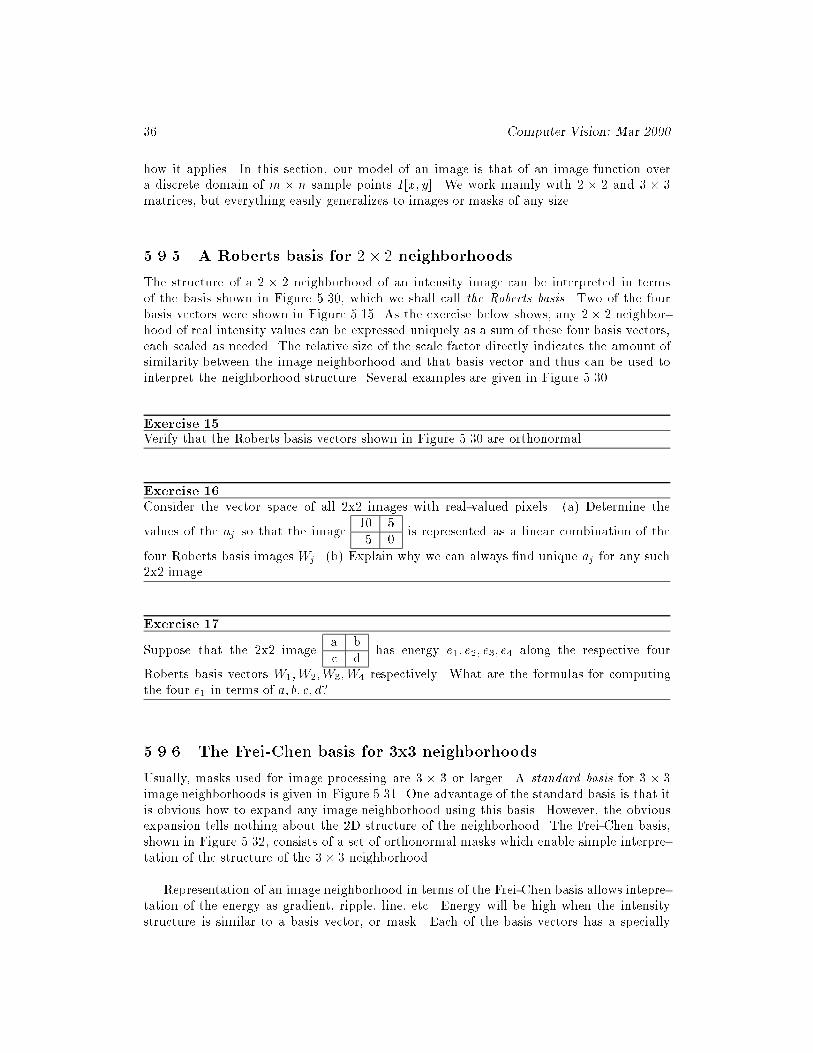
5.9.5 A Roberts basis for 2 � 2 neighborhoods
The structure of a 2 � 2 neighborhood of an intensity image can be interpreted in terms
of the basis shown in Figure 5.30, which we shall call the Roberts basis. Two of the four
basis vectors were shown in Figure 5.15. As the exercise below shows, any 2� 2 neighbor-
hood of real intensity values can be expressed uniquely as a sum of these four basis vectors,
each scaled as needed. The relative size of the scale factor directly indicates the amount of
similarity between the image neighborhood and that basis vector and thus can be used to
interpret the neighborhood structure. Several examples are given in Figure 5.30.
Exercise 15Verify that the Roberts basis vectors shown in Figure 5.30 are orthonormal.
Exercise 16
Consider the vector space of all 2x2 images with real-valued pixels. (a) Determine the
values of the aj so that the image10 5
5 0is represented as a linear combination of the
four Roberts basis images Wj . (b) Explain why we can always �nd unique aj for any such
2x2 image.
Exercise 17
Suppose that the 2x2 imagea b
c dhas energy e1; e2; e3; e4 along the respective four
Roberts basis vectors W1;W2;W3;W4 respectively. What are the formulas for computing
the four e1 in terms of a; b; c; d?
5.9.6 The Frei-Chen basis for 3x3 neighborhoods
Usually, masks used for image processing are 3 � 3 or larger. A standard basis for 3 � 3
image neighborhoods is given in Figure 5.31. One advantage of the standard basis is that it
is obvious how to expand any image neighborhood using this basis. However, the obvious
expansion tells nothing about the 2D structure of the neighborhood. The Frei-Chen basis,
shown in Figure 5.32, consists of a set of orthonormal masks which enable simple interpre-
tation of the structure of the 3� 3 neighborhood.
Representation of an image neighborhood in terms of the Frei-Chen basis allows intepre-
tation of the energy as gradient, ripple, line, etc. Energy will be high when the intensity
structure is similar to a basis vector, or mask. Each of the basis vectors has a specially

Shapiro and Stockman 37
Roberts basis: W1 =12
1 1
1 1W2 =
1p2
0 1
-1 0W3 =
1p2
+1 0
0 -1W4 =
12
-1 1
1 -1
Constant region:5 5
5 5= 20
2(12
1 1
1 1) = 10W1 � 0W2 � 0W3 � 0W4
Step Edge:-1 +1
-1 +1= 0W1 � 2p
2W2 � 2p
2W3 � 0W4
Step Edge:+1 +1
-3 +1= 0W1 � 4p
2W2 � 0W3 � �4
2W4
Line:0 8
8 0= 8W1 � 0W2 � 0W3 � 8W4
Figure 5.30: (Top row) A basis for all 2x2 images which contains the two Roberts gradient
masks; (row 2) constant region is a multiple of the constant image; (row 3) vertical step
edge has energy only along the gradient masks; (row 4) diagonal step edge has most energy
along the matching gradient mask; (row 5) line pattern has energy along constant maskW1
and line mask W4 .
1 0 0
0 0 0
0 0 0
0 1 0
0 0 0
0 0 0
0 0 1
0 0 0
0 0 0
...
0 0 0
0 0 0
0 1 0
0 0 0
0 0 0
0 0 1
Nine \standard" basis vectors for the space of all 3x3 matrices.
9 5 0
5 0 0
0 0 0
= 91 0 0
0 0 0
0 0 0
+50 1 0
0 0 0
0 0 0
+50 0 0
1 0 0
0 0 0
Figure 5.31: Any 3�3 matrix can be represented as a sum of no more than 9 scaled standard
matrices: (top row) nine basis vectors and (bottom row) representation of an example matrix
in terms of the basis.

38 Computer Vision: Mar 2000
gradient: W1 = 1=p8
1p2 1
0 0 0
-1 �p2 -1
W2 = 1=p8
1 0 -1p2 0 �
p2
1 0 -1
ripple: W3 = 1=p8
0 -1p2
1 0 -1
�p2 1 0
W4 = 1=p8
p2 -1 0
-1 0 1
0 1 �p2
line: W5 = 1=2
0 1 0
-1 0 -1
0 1 0
W6 = 1=2
-1 0 1
0 0 0
1 0 -1
Laplacian: W7 = 1=6
1 -2 1
-2 4 -2
1 -2 1
W8 = 1=6
-2 1 -2
1 4 1
-2 1 -2
constant: W9 = 1=3
1 1 1
1 1 1
1 1 1
Figure 5.32: The Frei-Chen basis for the set of all 3x3 images with real intensity values.
designed structure. The basis vectors W1 andW2 are similar to the Prewitt and Sobel gra-
dient masks, while the basis vectors W7 and W8 are similar to the common 3x3 Laplacian
mask. The line masks will respond strongly to one-pixel wide lines passing through a 3x3
neighborhood, while the two ripple masks model two perpendicular waves with two peaks,
two troughs, and three zero-crossings. The elements of the vectors di�er slightly from the
masks that we formerly designed in isolation because of the requirement that the set be
orthogonal.
Algorithm 2 computes a binary image which detects intensity neighborhood structure
with signi�cant energy in a speci�ed subspace. To detect edges, one could select pixels by
their neighborhood energy along the basis vectors W1; W2, which would be indicated by
setting S = f1; 1; 0; 0; 0;0;0;0; 0g. An example of the calculations projecting the intensity
neighborhood on the Frei-Chen basis vectors is also given below.

Shapiro and Stockman 39
Detect neighborhoods with high energy in a selected subspace.
F[r; c] is an input intensity image; F is unchanged by the algorithm.
S is a bit vector such that S[j] = 1 if and only ifWj is included in the subspace of interest.
thresh is a threshold on the fraction of energy required.
noise is the noise energy level.
G[r; c] is the output image, a binary image where G[r; c] = 1 indicates that F[r; c] has
above threshold energy in the speci�ed subspace S.
procedure detect neighborhoods(F;G;S; thresh; noise);
ffor r := 0 to MaxRow - 1
for c := 0 to MaxCol - 1
fif [r,c] is a border pixel then G[r; c] := 0;
else G[r; c] := compute using basis ( F; r; c;S; thresh; noise);
g ;gprocedure compute using basis( IN; r; c; thresh; noise )
fN[r; c] is the 3x3 neighborhood centered at pixel [r,c] of IN[].
average energy := N[r; c] �W9;
subspace energy := 0.0;
for j := 1 to 8
fif (S[j]) subspace energy := subspace energy + (N[r; c] �Wj)
2;
gif subspace energy < noise return 0;
if subspace energy/((N[r; c] �N[r; c])-average energy) < thresh return 0;
else return 1;
g
Algorithm 2: Compute detection image G[r; c] from input image F[r; c] and subspace S.

40 Computer Vision: Mar 2000
Example of representing an intensity neighborhood using the Frei-Chen
basis.
Consider the intensity neighborhood N =
10 10 10
10 10 5
10 5 5
We �nd the component of this vector along each basis vector using the dot product
as before. Since the basis is orthonormal, the total image energy is just the sum
of the component energies and the structure of N can be interpreted in terms of
the components.
N �W1 =5 + 5
p2p
8� 4:3; energy � 18
N �W2 =5 + 5
p2p
8� 4:3; energy � 18
N �W3 = 0; energy = 0
N �W4 =5p2� 10p8
� �1; energy � 1
N �W5 = 0; energy = 0
N �W6 = 2:5; energy � 6
N �W7 = 2:5; energy � 6
N �W8 = 0; energy = 0
N �W9 = 25; energy = 625
The total energy in N is N � N = 675, 625 of which is explained just by the
average intensity level along W9. The energy along all other components is 50
of which 36, or 72%, is along the gradient basis vectors W1 and W2. Thus, the
neighborhood center would be marked as a detected feature in case the gradient
subspace is of interest.
Exercise 18Verify that the set of nine vectors shown in Figure 5.32 is an orthonormal set.
Exercise 19
(a) Represent the intensity neighborhood
0 0 1
0 1 0
1 0 0
in terms of the basis vectors shown
in Figure 5.32. Is all the energy distributed along the line basis vectors W5 and W6? (b)
Repeat the question (a) for the intensity neighborhood
0 1 0
0 1 0
0 1 0
.

Shapiro and Stockman 41
Exercise 20
(a) Represent the intensity neighborhood
10 10 10
10 20 10
10 10 10
in terms of the basis vectors shown
in Figure 5.32. Is all the energy distributed along certain basis vectors as you expect? (b)
Would the interpretation of the intensity neighborhood
0 0 0
0 1 0
0 0 0
be di�erent: why or
why not? (c) What kind of image neighborhoods give responses to only W7 and W8?
Exercise 21Write a program to implement the detection of pixels using the Frei-Chen basis as outlined
in the algorithm above. Allow the user of the program to input the subspace S of interest
as a string of 9 bits. The user should also be able to input the noise energy level and the
threshold determining the minimum energy required in the selected subspace. Test your
program on some real images and also on some test patterns such as those in the exercises
above.
5.10 *Convolution and Cross Correlation
The previous sections showed how many useful detections can be performed by matching
a mask or pattern image to an image neighborhood. Also, we saw that image smoothing
could be put in the same framework. In this section, we give de�nitions for the important
operations of cross correlation and convolution, which formalize the notion of moving a mask
around the image and recording the dot product of the mask with each image neighborhood.
5.10.1 De�ning operations via Masks
We begin by rede�ning simple image smoothing as the cross correlation of the image with
a smoothing mask. A boxcar �lter computes the ouptut image pixel as an equal weighting
of a neighborhood of pixels of the corresponding input image pixel. This is equivalent to
performing a dot product of an m�n image pattern of weights 1mn
as is shown in Figure 5.33
for a 3 � 3 mask. Assuming that m and n are both odd and the division by 2 ignores the
remainder, Equation 5.25 de�nes the dot product used to compute the value of the output
pixel G[x; y] from input image F [] using mask H[]. In this formulation, mask H is centered
at the origin so that H[0; 0] is the center pixel of the mask: it is obvious how H is used to
weight the pixels from the neighborhood of F[x;y]. An alternate formulation convenient to
compute all output pixels of G results from a simple change of variables in Equation 5.25
yielding Equation 5.26 which can use masks H[] with even dimensions.

42 Computer Vision: Mar 2000
19 Definition The cross correlation of image F [x; y] and mask H[x; y] is de-�ned as
G[x; y] = F [x; y]H[x; y]
=
w=2Xi=�w=2
h=2Xj=�h=2
F [x+ i; y + j]H[i; j]
(5.25)
For implementation of this computational formula:
mask H[x; y] is assumed to be centered over the origin, so negative coordinates
make sense;
image F [x; y] need not be centered at the origin;
result G[x; y] must be de�ned in an alternate manner when H[] does not
completely overlap F [].
An alternate formulation does not require a mask with odd dimensions, but
should be viewed as an entire image transformation and not just an operation
centered on pixel G[x; y].
G[x; y] =
w�1Xi=0
h�1Xj=0
F [x+ i; y + j]H[i; j] (5.26)
Exercise 22
Suppose that an image F[] has all 0 pixels except for a single 1 pixel at the image cen-
ter. What output image G[] results from convolving F[] with the 3 � 3 boxcar shown in
Figure 5.33?
Exercise 23
Design a single mask to detect edge elements making an angle of 300 with the X-axis. The
mask should not respond strongly to edge elements of other directions or to other patterns.
Exercise 24 Corner detection
(a) Design a set of four 5� 5 masks to detect the corners of any rectangle aligned with the
image axes. The rectangle can be brighter or darker than the background. (b) Are your
masks orthogonal? (c) Specify a decision procedure to detect a corner and justify why it
would work.
5.10.2 The Convolution Operation
20 Definition The convolution of functions f(x; y) and h(x; y) is de�ned as
g(x; y) = f(x; y) ? h(x; y) �Z +1
x0=�1
Z +1
y0=�1f(x0; y0)h(x� x0; y � y0)dx0dy0 (5.27)

Shapiro and Stockman 43
36 36 36 36 36 3636 36 45 45 54 5436 36 45 54 54 5436 45 54 54 63 6336 45 54 63 63 7245 45 63 63 72 72
1/9 1/9 1/91/9 1/9 1/91/9 1/9 1/9
36 36 36 36 36 3636 38 41 45 47 5436 41 46 52 55 5436 43 50 56 60 6336 47 54 61 65 7245 45 63 63 72 72
x =
F[r,c]
Input Image
Mask overlaid withImage at [r,c] Mask or Kernel
H[-1,-1] H[0,-1] H[1,-1]
H[-1,0] H[0,0] H[1,0]
H[-1,1] H[0,1] H[1,1]
G[r,c]
Output Image
Figure 5.33: Smoothing an image using a 3� 3 boxcar �lter can be viewed as computing a
dot product between every input image neighborhood and a mask (boxcar) that is a small
image of equal values.
Convolution is closely related to cross correlation and is de�ned formally in terms of
continuous picture functions in Equation 5.27. In order for the integrals to be de�ned and
to have practical use, the 2D image functions f(x; y) and h(x; y) should have zero values
outside of some �nite rectangle in the xy�plane and have �nite volume under their surface.
For �ltering, kernel function h(x; y) will often be zero outside some rectangle that is much
smaller than the rectangle that supports f(x; y). For a global analysis of the spatial fre-
quency of f , the rectangle supporting h will include all of the support of f . More details are
given in the optional section of Fourier analysis below. Figure 5.34 shows an interpretation
of steps in computing the value of g(x) from the two functions being convolved in the case of
1D signals. Kernel function h(x) is �rst ipped about the origin and then translated to the
point x at which g(x) is being computed. g(x) is then computed by integrating the products
of the input function f(x0) times the relocated kernel h(x0 � x); since, that function is zero
outside of the interval [a; b], integration can be con�ned to this �nite interval. Convolution
is easily carried out with digital images by using discrete sums of products instead of the
continuous integrals de�ned above.
Cross correlation translates the mask or kernel directly to the image point [x; y] with-
out ipping it; otherwise it is the same operation used in convolution. Conceptually, it is
easier not to have to think of ipping the kernel, but rather just placing it at some image
location. If the kernel is symmetric so that the ipped kernel is the same as the original
kernel, then the results of convolution and correlation will be identical. While this is the
case for smoothing masks and other isotropic operators, many edge detection masks are

44 Computer Vision: Mar 2000
Exercise 25 Rectangle detection
Use the corner detection procedure of the previous exercise to implement a program that
detects rectangles in an image. (Rectangle sides are assumed to align with the sides of
the image.) The �rst step should detect candidate rectangle corners. A second step should
extract subsets of four candidate corners that form a proper rectangle according to geometric
constraints. An optional third step might further check the four corners to make sure that
the intensity within the candidate rectangle is uniform and contrasting with the backgorund.
What is the expected behavior of your program if it is given a noisy checkerboard image?
Test your program on a noisy checkerboard, such as in Figure 5.7 and an image of a building
with rectangular windows, such as in Figure 5.42.
x x
x
h ( x ) h ( - x )
a b
x’
x’
f ( x )
0.5
-0.5 0.5 x
h ( x’ - x )
h ( x’ - x )
g ( x ) = f ( x’ ) h ( x’ - x ) dx’
a
b
Figure 5.34: Computing convolution g(x) of signal f(x) with kernel h(x) denoted g(x) =
f(x) ? h(x). For any domain point x, kernel h is ipped and then translated to x; then,
g(x) is computed by summing all the products of f(x) and the values of the ipped and
translated h.
x
y
image F[x, y]
H[ 0, 0 ]
G[x, y] = F[x, y] x H[x, y]
x
y
[x, y]
H[ -w/2, -h/2 ][ x -w/2 , y -h/2 ]
[ x + w/2 , y + h/2 ]
mask H[x, y]
H[w/2, h/2]
Figure 5.35: Computing the cross correlation G[x; y] of image F [x; y] with mask H[x; y]:
G[x; y] = F [x; y]H[x; y]. To compute G[x; y], the maskH[x; y] is centered on input image
point F [x; y] to sum all the products of image values of F and the corresponding overlaid
weights of H.

Shapiro and Stockman 45
5 5 5 5 5 5
5 5 5 5 5 5
5 5 10 10 10 10
5 5 10 10 10 10
5 5 5 10 10 10
5 5 5 5 10 10
0 -1 0
-1 4 -1
0 -1 0
=
0 0 0 0 0 0
0 0 -5 -5 -5 0
0 -5 10 5 5 0
0 -5 10 0 0 0
0 0 -10 10 0 0
0 0 0 0 0 0
Cross correlation with a LOG mask produces zero-crossings at boundaries.
5 5 5 5 5 5
5 5 5 5 5 5
5 5 10 10 10 10
5 5 10 10 10 10
5 5 5 10 10 10
5 5 5 5 10 10
-1 0 +1
-1 0 +1
-1 0 +1
=
0 0 0 0 0 0
0 5 5 0 0 0
0 10 10 0 0 0
0 10 15 5 0 0
0 5 10 10 5 0
0 0 0 0 0 0
Cross correlation with column derivative mask detects column boundaries.
5 5 5 5 5 5
5 5 5 5 5 5
5 5 10 10 10 10
5 5 10 10 10 10
5 5 5 10 10 10
5 5 5 5 10 10
+1 +1 +1
0 0 0
-1 -1 -1
=
0 0 0 0 0 0
0 -5 -10 -15 -15 0
0 -5 -10 -15 -15 0
0 5 5 5 0 0
0 5 10 10 5 0
0 0 0 0 0 0
Cross correlation with row derivative mask detects column boundaries.
Figure 5.36: Cross correlation of an image with various masks to enhance regions boundaries:
(top) second derivative operator produces a zero-crossing at boundaries; (center) column ( x
) derivative operator detects changes across columns; (right) column ( y ) derivative operator
detects changes across rows.

46 Computer Vision: Mar 2000
asymmetric. Despite the formal di�erence between convolution and cross correlation, those
who do image processing often loosely refer to either operation as \convolution" because
of their similarity. The many masks used in this chapter, and others, have been presented
assuming that they would not be ipped before being applied to an image. Normalized crosscorrelation will normalize by dividing G[x; y] by the magnitudes of both F [x; y] and H[x; y]
so that the result can be interpreted as a result of matching the structure of F with the
structure ofH that is independent of scale factors, as has been discussed in previous sections.
Exercise 26
Given H =
1 0 -3
0 4 0
-3 0 1
and F =
5 5 5 5 5 5
5 5 5 5 8 8
5 5 5 8 8 8
5 5 8 8 8 8
8 8 8 8 8 8
,
compute G = F H.
Exercise 27 Point spread
Given kernel H =
1 2 1
2 5 2
1 2 1
, what is the result of convolving it with an image F [x; y]
which has F [x0; y0] = 1 and all other pixels 0?
Exercise 28
Suppose that function h(x) takes value 1 for �1=2 � x � 1=2 and is zero elsewhere, and
suppose that function f(x) takes value 1 for 10 � x � 20 and zero elsewhere. (a) Sketch
the two functions f and h. (b) Compute and sketch the function g(x) = f(x) ? h(x). (c)
Compute and sketch the function g(x) = h(x) ? h(x).
5.10.3 Possible parallel implementations
One can see from the de�nition of convolution, that g(x1; y1) can be computed indepen-
dently of g(x2; y2); in fact, all the integrations can be done at the same time in parallel.
Also, each integration computing an individual value g(x; y) can form all of the products
simultaneously, enabling a highly parallel system. Various computer architectures can be
envisioned to perform all or some operations in parallel.
5.11 *Analysis of spatial frequency using sinusoids
Fourier analysis is very important in signal processing; its theory and practice �lls many
books. We give only a brief snapshot here, building on the notions of a vector space already
introduced.

Shapiro and Stockman 47
Exercise 29The pointilist school of painters created their paintings by dabbing their paintbrush per-
pendicularly on the canvas and creating one dab/point of color at a time. Each dab is
similar to a single pixel in a digital image. The human viewer of the artwork would stand
back and a smooth picture would be perceived. Implement a program to do pointilist art.
The program should present a palette of colors and some other options, such as choosing
paintbrush size or whether '+' or 'XOR' would be used for dabbing, etc. When your pro-
gram is working, create a painting of a starry night. Your program should work with an
external �le representing the painting in progress so that a user could save the session for
later continuation.
Exercise 30Implement a program to convolve a mask with an image. The program should read both
the image and mask from input �les in the same format. Perhaps you can test it on the
artwork produced by the program from the previous exercise.
Exercise 31
Suppose in the search for extra terrestrial intelligence (SETI) deep space is scanned with
the hope that interesting signals would be found. Suppose signal S is a concatenation of
the �rst 100 prime numbers in binary form and that R is some received signal that is much
longer than S. Assume that R has noise and has real valued coordinates. To �nd if S is
embedded in R, would cross correlation or normalized cross correlation work? Why?
-150
-100
-50
0
50
100
150
0 100 200 300 400 500
c3(x) : 100 cos( 2 PI 3X / 512)
c3(x)
-150
-100
-50
0
50
100
150
0 100 200 300 400 500
c16(x) : 30 cos( 2 PI 16X / 512)
c16(x)
-150
-100
-50
0
50
100
150
0 100 200 300 400 500
c30(x) : 20 cos( 2 PI 30X / 512)
c30(x)
-150
-100
-50
0
50
100
150
0 100 200 300 400 500
sum(x) : c3(x) + c16(x) + c30(x)
sum(x)
-150
-100
-50
0
50
100
150
0 100 200 300 400 500
sum(x) : c3(x) + c16(x)
sum(x)
Figure 5.37: (Top row) Three sinusoids, 100cos(2� 3x512
), 30cos(2� 16x512
) and 20cos(2� 30x512
);
(bottom row left) sum of all three and (bottom row right) sum of �rst two.

48 Computer Vision: Mar 2000
Figure 5.38: Di�erent sinusoidal picture functions in the spatial domain [x; y]: The top left
image was generated by the formula 100cos(2�(16x=512))+100 and has 16 cycles along the
x-axis. The bottom right image was generated by the formula 100cos(2�(12y=512)) + 100
and has 12 cycles along the y-axis. The bottom left image was generated by the formula
100cos(2�(16x=512 + 12y=512)) + 100: note how the waves of the bottom left image align
with those of the top left and bottom right. The Fourier power spectrum is shown at the
top right.
The mathematician Fourier imagined the surface of the sea as a sum of sine waves. Large
waves caused by the tide or ships had long wavelengths (low frequency), while smaller waves
caused by the wind or dropped objects, etc. had short wavelengths (high frequency). The
top row of Figure 5.37 shows three pure waves of 3, 16, and 30 cycles across a 1D space
of x 2 [0; 512]: in the bottom row are two functions, one which sums all three waves and
one which sums only the �rst two. Similar sets of waves can be used to create 2D picture
functions or even 3D density functions.
The Fourier theory in analysis shows how most real surfaces or real functions can be
represented in terms of a basis of sinusoids. The energy along the basis vectors can be
interpreted in terms of the structure of the represented surface (function). This is most
useful when the surface has repetitive patterns across large regions of the surface; such as
do city blocks of an aerial image of an urban area, waves on a large body of water, or the
texture of a large forest or farm �eld. The idea is to expand the entire image, or various
windows of it, using a Fourier basis and then �lter the image or make decisions about it
based on the image energy along various basis vectors. For example, high frequency noise
can be removed by subtracting from the image all the components along high frequency
sine/cosine waves. Equivalently, we can reconstruct our spatial image by adding up only
the low frequency waves and ignoring the high frequency waves.
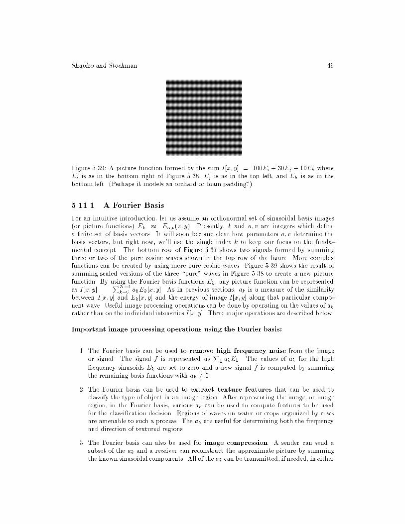
Shapiro and Stockman 49
Figure 5.39: A picture function formed by the sum I[x; y] = 100Ei + 30Ej + 10Ek where
Ei is as in the bottom right of Figure 5.38, Ej is as in the top left, and Ek is as in the
bottom left. (Perhaps it models an orchard or foam padding?)
5.11.1 A Fourier Basis
For an intuitive introduction, let us assume an orthonormal set of sinusoidal basis images
(or picture functions) Ek � Eu;v(x; y). Presently, k and u; v are integers which de�ne
a �nite set of basis vectors. It will soon become clear how parameters u; v determine the
basis vectors, but right now, we'll use the single index k to keep our focus on the funda-
mental concept. The bottom row of Figure 5.37 shows two signals formed by summing
three or two of the pure cosine waves shown in the top row of the �gure. More complex
functions can be created by using more pure cosine waves. Figure 5.39 shows the result of
summing scaled versions of the three \pure" waves in Figure 5.38 to create a new picture
function. By using the Fourier basis functions Ek, any picture function can be represented
as I[x; y] =PN�1
k=0 akEk[x; y]. As in previous sections, ak is a measure of the similarity
between I[x; y] and Ek[x; y] and the energy of image I[x; y] along that particular compo-
nent wave. Useful image processing operations can be done by operating on the values of akrather than on the individual intensities I[x; y]. Three major operations are described below.
Important image processing operations using the Fourier basis:
1. The Fourier basis can be used to remove high frequency noise from the image
or signal. The signal f is represented asP
k akEk. The values of ak for the high
frequency sinusoids Ek are set to zero and a new signal f̂ is computed by summing
the remaining basis functions with ak 6= 0.
2. The Fourier basis can be used to extract texture features that can be used to
classify the type of object in an image region. After representing the image, or image
region, in the Fourier basis, various ak can be used to compute features to be used
for the classi�cation decision. Regions of waves on water or crops organized by rows
are amenable to such a process. The ak are useful for determining both the frequency
and direction of textured regions.
3. The Fourier basis can also be used for image compression. A sender can send a
subset of the ak and a receiver can reconstruct the approximate picture by summing
the known sinusoidal components. All of the ak can be transmitted, if needed, in either

50 Computer Vision: Mar 2000
order of energy, or in order of frequency: the receiver can terminate the transmission
at any time based on the content received up to that point.
Our goal here is to produce a useful basis of picture functions and an understanding
of how to use it in practice. Some important mathematical background using continuous
functions is needed. For this development, lets assume that the origin of our coordinate
system is at the center of our picture function, which is de�ned for a square region of the
xy-plane. When we proceed to a digital version, the picture will be represented by digital
image I[x; y] with N2 samples. First, we establish a set of sinusoids of di�erent frequency
as an orthogonal basis for continuous signals f . If m;n are any two di�erent integers,
then the two cosine waves with these frequency parameters are orthogonal over the interval
[��; �]. The reader should work through the following exercises to verify that the function
set f1; sin(mx); cos(nx); : : :g is an orthogonal set of functions on [��; �]. The orthogonalityof the cosine waves follows from Equation 5.28, since sin(k�) = 0 for all integers k.
Z �
��cos(m�)cos(n�)d� =
sin(m � n)�
2(m� n)+sin(m + n)(��)
2(m+ n)
= 0 for m2 6= n2
(5.28)
N symmetrically spaced samples of these cosine functions will create a set of vectors
that will be orthogonal in the sense de�ned previously by the dot product.
Exercise 32
Consider the set of all continuous functions f de�ned on the interval x 2 [x1; x2]. Show
that this set of functions f; g; h; : : :, together with scalars a; b; c; : : : forms a vector space by
arguing that the following properties hold.
f � g = g � f (f � g)� h = f � (g � h)
c(f � g) = cf � cg (a+ b)f = af � bf
(ab)f = a(bf) 1f = f
0f = 0
5.11.2 2D Picture Functions
21 Definition The complex valued picture function
Eu;v(x; y) � e�j 2�(ux+vy)
= cos(2�(ux+ vy)) � jsin(2�(ux + vy))
(5.30)
where u and v are spatial frequency parameters as shown in Figure 5.38 and j =p�1.
Using a complex value is a convenience that allows us to separately account for both a
cosine and sine wave of the same frequency: the sine wave has the same structure as the
Shapiro and Stockman 51
Exercise 33
For the space of continuous functions of x 2 [x1; x2], as in the exercise above, de�ne a dot
product and corresponding norm as follows.
f � g =
Z b
a
f(x)g(x)dx ; kfk =pf � f (5.29)
Argue why the following four properties of a dot product hold.
(f � g) � h = (f � g) + (g � h)f � f � 0
f � f = 0() f = 0
f � g = g � f(cf) � g = c(f � g)
Exercise 34 Odd and even functions
A function is an even function i� f(�x) = f(x) and a function is an odd function if f(�x) =�f(x). (a) Show that cos(mx) is an even function and that sin(nx) is an odd function,
where m;n are nonzero integers. (b) Let f and g be odd and even continuous functions on
[�L;L], respectively. Argue thatR L�L f(x)g(x)dx = 0.
Exercise 35Using the de�nition of the dot product given in Exercise 33 above, show that the set of
sinusoidal functions fk de�ned below are orthogonal on the interval [��; �].f0(x) = 1; f1(x) = sin(x); f2(x) = cos(x); f3(x) = sin(2x); f4(x) = cos(2x); f5(x) =
sin(3x); f6(x) = cos(3x); : : :

52 Computer Vision: Mar 2000
cosine wave but is 1/4 wavelength out of phase with the cosine wave. When one of these
basis functions correlates highly with a picture function, it means that the picture function
has high energy in frequency u; v. The Fourier transform, converts a picture function into
an array of these correlations. We start with the integral form and then give the discrete
summation for digital images below.
22 Definition The 2D Fourier Transform transforms a spatial function f(x; y) into theu; v frequency domain.
F (u; v) �Z 1
�1
Z 1
�1f(x; y)Eu;v(x; y)dxdy
=
Z 1
�1
Z 1
�1f(x; y)e�j 2�(ux+vy)dxdy
(5.31)
The function f must be well-behaved; speci�cally, picture functions have the following
properties which make the above formula well-de�ned.R1�1R1�1 j f(x; y) jdxdy is �nite; moreover, f(x; y) = 0 outside of some rectangle R so the
in�nite limits in the formula can be replaced by the limits of R. Also, f has a �nite number
of extrema and no in�nite discontinuities in R.
Exercise 36
What is the special meaning of F (0; 0), where F (u; v) is the Fourier transform of picture
function f(x; y)?
Often, we want to work with the power spectrum, which combines energy from sine and
cosine waves of the same frequency components u; v. A power spectrum is shown at the top
right of Figure 5.38.
23 Definition The Fourier power spectrum is computed as
P (u; v) � ( Real(F (u; v))2+ Imaginary(F (u; v))
2)1=2 (5.32)
Figure 5.40 shows how the actual wavelength of a 2D sinusoid relates to the wavelengths
projected along each axis. u is the frequency along the X-axis in cycles per unit length and
1=u is the wavelength. v is the frequency along the Y -axis and 1=v is the wavelength. � is
the wavelength of the sinusoid along its natural axis, or direction of travel. By computing
the area of the triangle shown at the right in Figure 5.40 in two di�erent ways, we obtain
the following formula which will help us interpret what the power spectrum tells us about
the frequency content of the original image.
�p(1=u)2 + (1=v)2 = (1=u)(1=v)
� =1p
u2 + v2(5.33)
Let's assume that the both the width and height of our picture have length 1. In
Figure 5.38 there are u = 16 cycles across the width of the picture, so the wavelength is
1=u = 1=16. Similarly, we have 1=v = 1=12. Applying the formula in Equation 5.33, we
obtain � = 1=20. By counting the number of waves in Figure 5.38 at the bottom left, we see

Shapiro and Stockman 53
X
Y
λ
λ
λ
λ
1 / u
1v
A
BC
1
1
λ
v
uC
A
B
Figure 5.40: Relationships among the wavelengths 1=u0 and 1=v0 of a sinusoid intercepted
by the X and Y axes and the wavelength � of the 2D wave.
��������
������������������
����������������������������
u u u
vvv
0u
1λ
θ
= 16
=120v
Figure 5.41: (Top row) three sinusoidal waves and (bottom row) their principle response in
the power spectrum.

54 Computer Vision: Mar 2000
Figure 5.42: Four images (above) and their power spectrums (below). The power spectrum
of the brick texture shows energy in many sinusoids of many frequencies, but the dominant
direction is perpendicular to the 6 dark seams running about 45 degrees with the X-axis.
There is noticable energy at 0 degrees with the X axis, due to the several short vertical
seams. The power spectrum of the building shows high frequency energy in waves along
the X-direction and the Y -direction. The third image is an aerial image of an orchard:
the power spectrum shows the rows and columns of the orchard and also the \diagnonal
rows". The far right image, taken from a phone book, shows high frequency power at about
60o with the X-axis, which represents the texture in the lines of text. Energy is spread
more broadly in the perpendicular direction also in order to model the characters and their
spacing.
27 waves across the 1.4 unit diagonal, yielding the expected frequency 27=1:4 � 20 along
the actual direction of the 2D wave.
Figure 5.41 shows the principle response in the power spectrum of the three sinusoidal
picture functions originally shown in Figure 5.38. The power spectrum at the top right of
Figure 5.38 actually shows heavy responses at three points, not just one. First of all, note
that F (0; 0) is just the total energy in f(x; y); since each sinusoid of Figure 5.38 has mean
of 100 and not 0, they have signi�cant average energy at zero frequency. Secondly, it is
evident from the de�ntion that P (�u;�v) = P (u; v), so the power spectrum is symmetric
about the origin u = 0; v = 0. Figure 5.42 shows the power spectrums of four real images.
The power spectrum need not be interpreted as an image, but rather as a 2D display
of the power in the original image versus the frequency parameters u and v. In fact, a
transform can be computed via optics, and thus it can be realized as a physical image.
In Chapter 2, there was brief mention of a sensor array partitioned into sectors and rings
(refer back to the \ROSA" con�guration in the relevant �gure from Chapter 2). Since the
power spectrum is symmetrical about the x-axis, as shown in Figure 5.42, the sectors can
be used to sample directional power, while the rings sample frequency bands without regard
to direction. Such sampling can also be done in software. In any case, if nr rings and nssectors are sampled, one obtains nr +ns features that may be useful for classi�cation of the
image neighborhood from which they were obtained.

Shapiro and Stockman 55
5.11.3 Discrete Fourier Transform
The discrete Fourier transform, or DFT, which is immediately applicable to digital images
is de�ned in Equation 5.34. We already know that a basis for the set of N �N images with
real intensity values must have N2 basis vectors. Each of these is determined by a pair of
frequency parameters u; v which range from 0 to N � 1 as used in the formulas below.
24 Definition The Discrete Fourier Transform (DFT) transforms an image of N �N spatial samples I[x; y] into an N � N array F [u; v] of coe�cents used in its frequencyreresentation.
F [u; v] � 1
N
N�1Xx=0
N�1Xy=0
I[x; y]e�2� j
N(xu+yv) (5.34)
To compute the single frequency domain element (\pixel") F [u; v], we just compute the
dot product between the entire image I[x; y] and a \mask" Eu;v[x; y], which is usually not
actually created, but computed implicitly in terms of u; v and the cos and sin functions as
needed. We also de�ne an inverse transform to transform a frequency domain representation
F [u; v] into a spatial image I[x; y]. Although it is useful to display the transform F as a 2D
image, it might be less confusing to insist that it is NOT really an image. We have used the
formal term frequency representation instead.
25 Definition The Inverse Discrete Fourier Transform(IDFT) transforms an N�Nfrequency representation F [u; v] into an N � N image I[x; y] of spatial samples.
I[x; y] � 1
N
N�1Xu=0
N�1Xv=0
F [u; v]e+2� j
N(ux+vy) (5.35)
If F [x; y] was computed by \forward" transforming I[x; y] in the �rst place, we want
the inverse transform to return to that original image. This property does hold for the
pair of de�nitions given above: proof is left to the guided exercises below. We �rst focus
the discussion on the practical use of the DFT & IDFT. For storage or communication
of an image, it might be useful to transform it into its frequency representation; the input
image can be recovered by using the inverse transform. In image processing, it is common to
perform some enhancement operation on the frequency representation before transforming
back to recover the spatial image. For example, high frequencies can be reduced or even
removed by reducing, or zeroing, the elements of F [u; v] that represent high frequency waves.
The convolution theorem below gives an elegant theoretical interpretation of this intuitive
process.
Exercise 37 Some basics about complex numbers
Use the de�nition ej! = cos ! + j sin !. (a) Show that (ej!)n = cos(n!) + j sin(n!).
(b) Show that x = ej2�kN is a solution to the equation xN � 1 = 0 for k = 0; 1; : : : ; N � 1.
(c) Let x0 = 1 = ej2�0N ; : : : ; xk = ej
2�kN be the N roots of the equation xN � 1 = 0. Show
that x1 + x2 + x3 + : : :+ xN�1 = 0.

56 Computer Vision: Mar 2000
Exercise 38 Proof of invertability of DFT/IDFT transforms
We want to prove that substituting the F [u; v] fromEquation 5.34 into Equation 5.35 returns
the exact original value I[x; y]. Consider the following summation, where x; y; s; t are integer
parameters in the range [0; N � 1] as used in the transform de�nitions:
G(x; y; s; t) =
N�1Xu=0
N�1Xv=0
ej 2�N
((x�s)u + (y�t)v):
(a) Show that if s = x and t = y, then G(x; y; s; t) =PN�1
u=0
PN�1v=0 1 = N2. (b) Show that
if s 6= x or t 6= y then G(x; y; s; t) = 0.
(c) Now show the major result that the inverse transform applied to the transform returns
the original image.
u
keep
remove
reduce or
keepkeep
v
reduce/remove reduce/remove
high pass bandpasslow pass
I [ x, y ] I’[x, y ]F[u, v] F’[u, v]F * F-1
Figure 5.43: Bandpass �ltering can be performed by a Fourier transformation into the
frequency domain (F[u;v]) followed by multiplication (*) by a bandpass �lter. The mul-
tiplication can set the \coe�cients" u; v of various frequencies to zero, as shown in the
top row. This modi�ed frequency representation is then inverse transformed to obtain the
modi�ed spatial image I0[x;y].

Shapiro and Stockman 57
5.11.4 Bandpass Filtering
Bandpass �ltering is a common image processing operation performed in the frequency do-
main and is sketched in Figure 5.43. The DFT is used to transform the image into its
frequency representation where the coe�cients for some frequencies are reduced, perhaps
to zero, while others are preserved. A sketch of the low pass �lter is given at the left of
Figure 5.43; intuitively, the high frequencies are erased and then the altered frequency rep-
resentation is inverse transformed via Equation 5.35 to obtain a smoothed version of the
original image. Instead of erasing elements of the frequency representation, we can take the
dot product of F [u; v] with a 2D Gaussian, which will weight the low frequency components
high and weight the high frequency components low. Figure 5.43 also shows how the fre-
quency representation would be altered to accomplish high pass and bandpass �ltering. The
theory of convolution below provides more insight to these operations.
5.11.5 Discussion of the Fourier Transform
The Fast Fourier Transform saves computational time by sharing common operations for
di�erent pairs of u; v and is usually used on square images of size 2m � 2m. Despite its
common use in image processing, the Fourier Transform can cause unwanted degradation
in local features of images because it is a global transform that uses all image pixels in
every computation of F [u; v]. For example, to represent hair or grass, or some other �ne
feature, high frequency waves must be used. First, such high frequencies might be �ltered
out as noise; however, even if not �ltered out, a high frequency response F [uh; vh] would
be computed by the dot product of a high frequency wave with the entire image. Since the
region of hair or grass would only be a small part of the entire image, the value of the dot
product could be high or low, depending on the rest of the image content. In the last ten
years, there has been a strong movement toward using wavelets instead of image-size waves.
Wavelets allow more sensitivity to local image variation, yet retain some major advantages
of using global sinusoids. JPEG and other picture compression schemes use cosine wave
representations on subimages to reduce the data size. Sometimes such compression must be
suppressed in order to preserve needed local image detail.
5.11.6 *The Convolution Theorem
In this section, we sketch a proof of the important convolution theorem , which tells us that
convolution of two functions in the spatial domain is equivalent to pointwise multiplication
of their frequency representations. This equivalence has great practical utility as has already
been seen.
Convolution Theorem:
If f(x; y) and h(x; y) are well-behaved functions of spatial parameters x; y, then F(f(x; y)?
h(x; y)) � F((f ?h)(x; y)) = F(f(x; y))F(h(x; y)) = F(u; v)H(u; v), where F is the Fourier
transform operator and ? is the convolution operator.
Before sketching a proof in the 1D case, we make the interpretation that is commonly
used in signal processing: convolution can be carried out without applying a mask h(x; y)
to all points of an image f(x; y).

58 Computer Vision: Mar 2000
Filter image f(x; y) with mask h(x; y)
(1) Fourier transform the image f(x; y) to obtain its frequency rep. F (u; v).
(2) Fourier transform the mask h(x; y) to obtain its frequency rep. H(u; v)
(3) multiply F (u; v) and H(u; v) pointwise to obtain F 0(u; v)(4) apply the inverse Fourier transform to F 0(u; v) to obtain the �ltered image f 0(x; y).
Algorithm 3: Filtering image f(x; y) with mask h(x; y) using the Fourier transform
For commonly used �lters h, the transform H is likely to be available either in closed
functional form or as a stored array in memory, thus short cutting step (2). Signal process-
ing texts typically contain a table of transform pairs < h;H > described both graphically
and in functional form so that the user can select a �lter with appropriate properties. We
now sketch a proof of the convolution theorem for the 1D case; these same steps can be
followed for the 2D case. An intermediate step is to show what happens to the transform
when the function is shifted.
Shift Theorem: F(f(x � x0)) = e�j 2�ux0F(f(x))
By de�nition F(f(x � x0)) �R +1�1 f(x � x0)e
�j 2�uxdx.
Making the change of variable x0 = x� x0, we obtain
F(f(x � x0)) =
Z +1
�1f(x0)e�j 2�u(x0+x0)dx0 (5.36)
=
Z +1
�1e�j 2�ux0f(x0)e�j 2�ux0dx0
= e�j 2�ux0F(f(x));
since the �rst factor is constant with respect to the variable of integration x0. Note that
j e�j 2�ux0 j2 = cos2(2�ux0) + sin2(2�ux0) = 1; (5.37)
so shifting the function does not change the energy of f(x) or F(u).
We can now use the above result to sketch the proof of the convolution theorem.
F((f ? h)(x)) �Z x=+1
x=�1(
Z t=+1
t=�1f(t)h(x � t)dt)e�j 2�uxdx: (5.38)
Using the good behavior assumed for functions f and h allows the order of integration to
be interchanged.
F((f ? h)(x)) =
Z t=+1
t=�1f(t) (
Z x=+1
x=�1h(x� t)e�j 2�uxdx) dt (5.39)
Using the shift theorem,Z x=+1
x=�1h(x� t)e�j 2�uxdx = e�j 2�utH(u); (5.40)

Shapiro and Stockman 59
where H(u) is the Fourier transform of h(x). We now have that
F((f ? h)(x)) =
Z t=+1
t=�1f(t)(e�j 2�utH(u)) dt
= H(u)
Z t=+1
t=�1f(t)e�j 2�ut dt
= H(u)F(u) = F(u)H(u) (5.41)
and the theorem is proved for the 1D case.
Exercise 39Follow the steps given above for proving the Shift Theorem and Convolution Theorem in
the 1D case and extend them to the 2D case.
5.12 Summary and Discussion
This was a long chapter covering several methods and many examples: it is important to
review major concepts. Methods were presented to enhance appearance of images for either
human consumption or for automatic processing. A few methods were given for remapping
intensity levels to enhance the appearance scene objects; it was shown that often some image
regions were improved at the expense of degrading others. The methods were presented only
for grey level images; however, most can be extended to color images, as you may already
know from using some image enhancing tool. Edge enhancement was also presented as a
method for human consumption. Hopefully, the artists toolbox has been expanded.
The most important concept of the chapter is that of using a mask or kernel to de�ne a
local structure to be applied throughout the image. Convolution and cross correlation are
two very powerful and related techniques which compute a result at I[x; y] by taking the
sum of the pointwise products of the input image intensity and a corresponding mask value.
These are linear operations that are pervasive in both theory and practice. Within this
context, it was shown that the response to a particular mask at a particular image point
(the correlation) is a measure of how similar the structure of the mask is to the structure of
the image neighborhood. This notion provides a practical method for designing masks, or
�lters, for a variety of tasks, such as smoothing, edge detection, corner detection, or even
texture detection.
There is a large literature on edge detection, and several di�erent schemes were covered
in this chapter. It should be clear that specifc edge detector output can be very useful for
particular machine vision tasks. The dream of many developers has not been realized, how-
ever | to produce a single uniform solution to the low level vision problem of representing
signi�cant object boundaries by some description based on detected edges. Perhaps it is
unrealistic to expect this. After all, given an image of a car, how does the low level system
know whether or not a car is present, is of interest, is moving or still, or whether we are
interested in inspecting for scratches in its paint or the �t of its doors versus just recog-
nizing the make? Many of the edgemaps extracted in our examples seemed very promising
for various applications. Indeed they are { many methods of subsequent chapters will be
based on representations built using edge input. The reader should not be overly optimistic,
however, because the reader has interpeted the images of this chapter using much higher

60 Computer Vision: Mar 2000
level organization and knowledge of objects and the world. The higher level methods that
we develop must be tolerant, because our edgemaps have gaps, noise, and multiple levels of
structure, which will challenge the algorithms that build from them.
5.13 References
Because few of the modern specialized journals existed when early work on image processing
and computer vision was done, research papers are scattered across many di�erent journals.
Larry Roberts published his seminal thesis work in recognition of 3D block-world objects in
1965. Part of that work was the detection of edges using the operator which now bears his
name. Roberts could not have anticipated the large amount of edge detection work which
would soon follow. Other early work was published by Prewitt in 1970 and Kirsch in 1971.
The Kirsch masks are now regarded as corner detectors rather than edge detectors. Recent
work by Shin et al (1998) supports the current popularity of the Canny step edge detector
(1986) by showing that it is one of the best in both performance and e�ciency, at least
in a structure-from-motion task. The paper by Huertas and Medioni (1986) takes a deep
practical look at implementing LOG �lters and shows how to use them to locate edges to
subpixel accuracy. The work on edge detection can easily be extended to 3D volume images
as has been done by Zucker and Hummel (1981).
The book by Kreider et al (1966) gives required linear algebra background focused on
its use in the analysis of functions, such as our picture functions: chapters 1,2 and 7 are
most relevant. Chapters 9 and 10 give background on Fourier series approximation of 1D
signals and are useful background for those wanting to explore the use of Fourier analysis
of 2D picture functions. One can consult the optics text by Hecht and Lajac (1974) for
Fourier interpretations of images as a superposition of waves. The book on algorithms by
Cormen et al (1990) gives two algorithms for selecting the i-th smallest of n numbers: the
theoretical bound on one of them is O(n) e�ort, which puts median �ltering in the same
theoretical complexity class as boxcar �ltering.
1. J. Canny (1986), A computational approach to edge detection, IEEE Trans. on Pattern
Analysis and Machine Intelligence, Vol. 8, No. 6 (Nov 1986)679-698.
2. T. Cormen, C. Leiserson, and R. Rivest (1990) Introduction to Algorithms, MIT Press,
Cambridge, Mass.
3. W. Frei and C-C. Chen (1977) Fast Boundary Detection: A Generalization and NewAlgorithm, IEEE Trans. on Computers, Vol. C-26, No. 10, (October 1977)pp988-998.
4. E. Hecht and A. Lajac (1974), Optics, Addison-Wesley. A. Huertas and G. Medioni
(1986),Detection of Intensity Changes with Subpixel Accuracy Using Laplacian-GaussianMasks IEEE-T-PAMI, Vol. 8, No. 5 (Sept 1986)651-664.
5. R. Kirsch (1971) Computer Determination of the Constituent Structure of BiologicalImages, Computers and Biomedical Research, Vol. 4, No. 3 (June 1971) pp315-
328.
6. D. Kreider, R. Kuller, D. Ostberg, and F. Perkins (1966)An Introduction to Linear
Analysis, Addison-Wesley, New York.

Shapiro and Stockman 61
7. J. Prewitt (1970) Object Enhancement and Extraction, in Picture Processing and
Psychopictorics, B. Lipkin and A. Rosenfeld (eds), Academic Press, N.Y. (1970)pp75-
149.
8. L. Roberts (1965) Machine Perception of Three-dimensional Solids, in Optical andElectro-Optical InformationProcessing, J. Tippett et al (eds) MIT Press,Cambridge,
Mass. (1965)pp159-197.
9. M. Shin, D. Goldgof, and K. Bowyer (1998) An Objective Comparison Methodologyof Edge Detection Algorithms using a Structure from Motion Task, in Empirical
Evaluation Techniques in Computer Vision, K. Bowyer and P. Philips, eds.,
IEEE Computer Society Press, Los Alamitos, CA.
10. S. Zucker and R. Hummel,A three-dimensional edge operator, IEEE-T-PAMI, Vol.3
(May 1981)324-331.