filter design workshop - engineeringece.uprm.edu/~domingo/teaching/inel5309/tutorial_filter... ·...
TRANSCRIPT

FILTER DESIGN WORKSHOP
Domingo Rodríguez
Automated Information Processing (AIP) Lab.
Electrical and Computer Engineering Department
INEL 4102, INEL 4095, INEL 4301, & INEL 5309
FILTER DESIGN WORKSHOP – January 17, 2017
Analog FiltersA Quick Basic Introduction
A More Detailed Introduction
Digital FiltersA Digital Filter Design Approach
Filter DesignFilter Design Using MATLAB
FDATool Design Technique
PSPICEFilter Simulation Using PSPICE
Workshop Outline
2

ANALOG FILTERS
3

Filters
Background:
. Filters may be classified as either digital or analog.
. are implemented using a digital computer
or special purpose digital hardware.
. may be classified as either passive or
active and are usually implemented with R, L, and C
components and operational amplifiers.
Courtesy of the University of Tennessee4
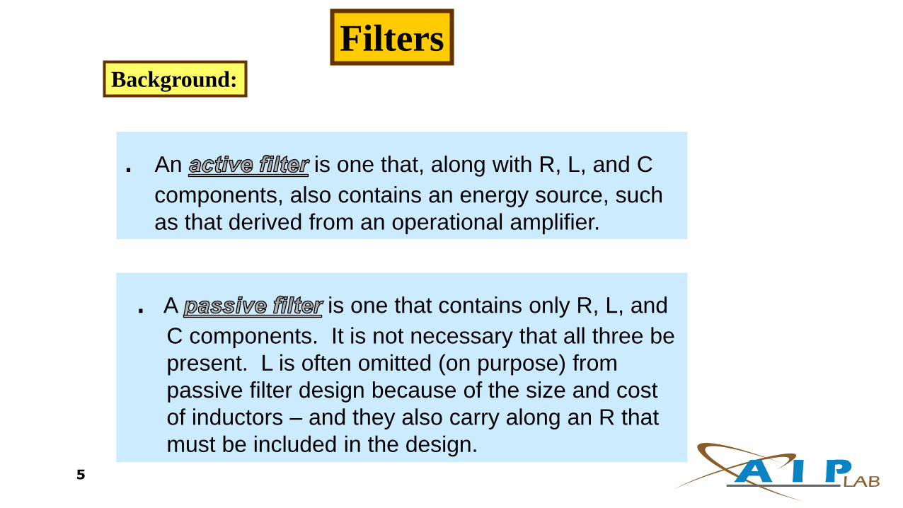
FiltersBackground:
. An is one that, along with R, L, and C
components, also contains an energy source, such
as that derived from an operational amplifier.
. A is one that contains only R, L, and
C components. It is not necessary that all three be
present. L is often omitted (on purpose) from
passive filter design because of the size and cost
of inductors – and they also carry along an R that
must be included in the design.
5
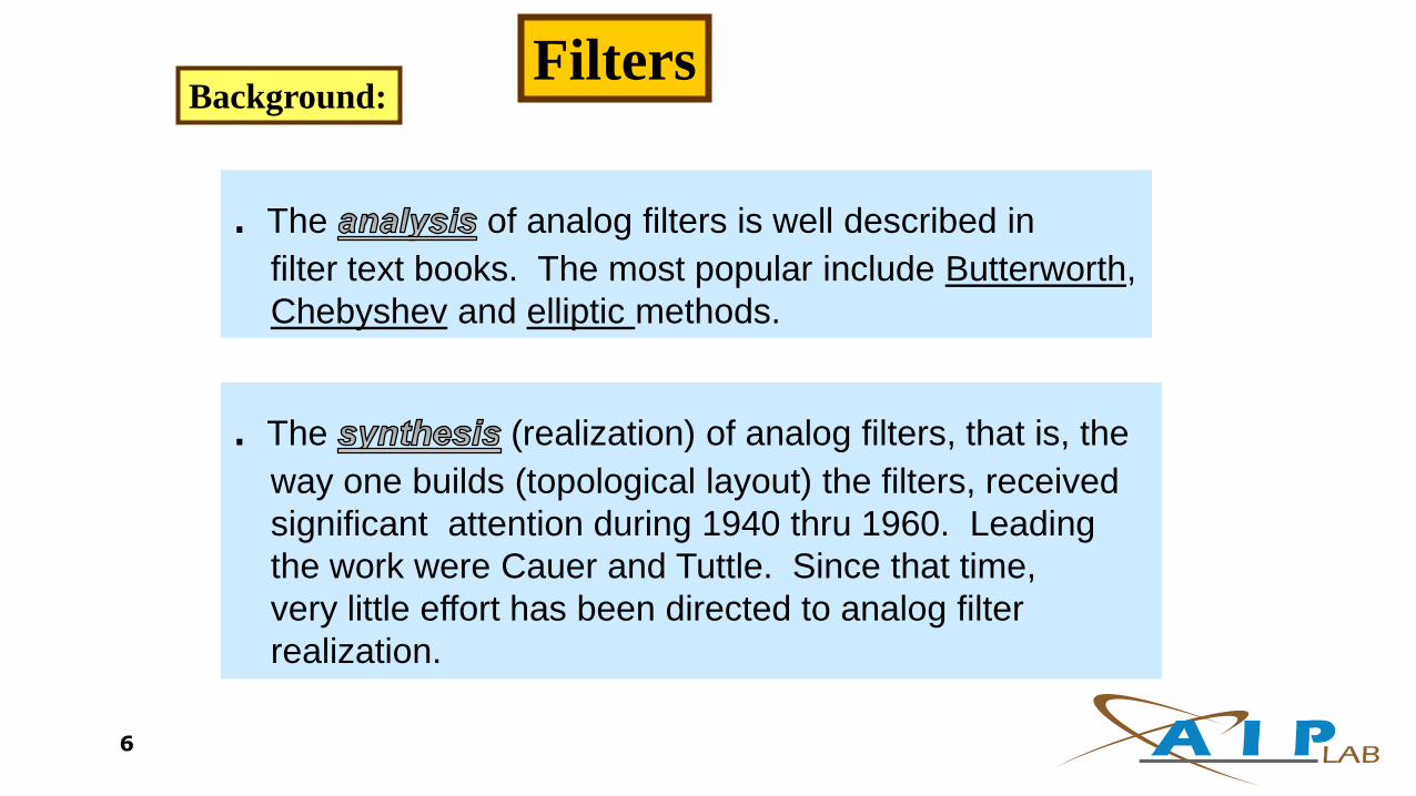
FiltersBackground:
. The (realization) of analog filters, that is, the
way one builds (topological layout) the filters, received
significant attention during 1940 thru 1960. Leading
the work were Cauer and Tuttle. Since that time,
very little effort has been directed to analog filter
realization.
. The of analog filters is well described in
filter text books. The most popular include Butterworth,
Chebyshev and elliptic methods.
6

FiltersBackground:
. Generally speaking, digital filters have become the focus
of attention in the last 40 years. The interest in digital
filters started with the advent of the digital computer,
especially the affordable PC and special purpose signal
processing boards. People who led the way in the work
(the analysis part) were Kaiser, Gold, and Rader.
. A digital filter is simply the implementation of an
equation(s) in computer software. There are no R, L,
C components as such. However, digital filters can also
be built directly into special purpose computers in
hardware form. But the execution is still in software.
7

FiltersBackground:
. In this course we will only be concerned with an
introduction to filters. We will look at both passive
and active filters; but, will concentrate on passive filters.
. We will not cover any particular design or realization
methods in detail; but, rather use our understanding of
poles and zeros in the s-plane, for basic designs.
. All EE and CE undergraduate students should take a
course in digital filter design, as an opinion.
8

Passive Analog Filters
Background: Four types of filters - “Ideal”
lowpass highpass
bandpass bandstop
9

Background: Realistic Filters:
lowpass highpass
bandpass bandstop
Passive Analog Filters
10

Passive Analog Filters
Background:
It will be shown later that the ideal
filter, sometimes called a “brickwall”
filter, can be approached by making the
order of the filter higher and higher.
The order here refers to the order of the
polynomial(s) that are used to define the
filter. MATLAB examples will be given later
to illustrate this.
11

Passive Analog Filters
Low Pass Filter Consider the circuit below.
R
CVI VO
+
_
+
_
1( ) 1
1( ) 1OV jw jwC
V jw jwRCRi
jwC
Low pass filter circuit
12

Passive Analog Filters
Low Pass Filter
0 dB
1
0
1/RC
1/RC
Bode
Linear Plot
.-3 dB
x0.707
Passes low frequencies
Attenuates high frequencies
13

Passive Analog Filters
High Pass Filter Consider the circuit below.
C
RVi VO
+
_
+
_
( )1( ) 1
OV jw jwRCRV jw jwRC
RijwC
High Pass Filter
14

Passive Analog Filters
High Pass Filter
0 dB
.
. -3 dB
0
1/RC
1/RC
1/RC
10.707
Bode
Linear
Passes high frequencies
Attenuates low frequencies
x
15

Passive Analog Filters
Bandpass Filter Consider the circuit shown below:
C L
RViVO
+
_
+
_
When studying series resonant circuit we showed that;
2
( )
1( )O
i
RsV s L
RV s s sL LC
16
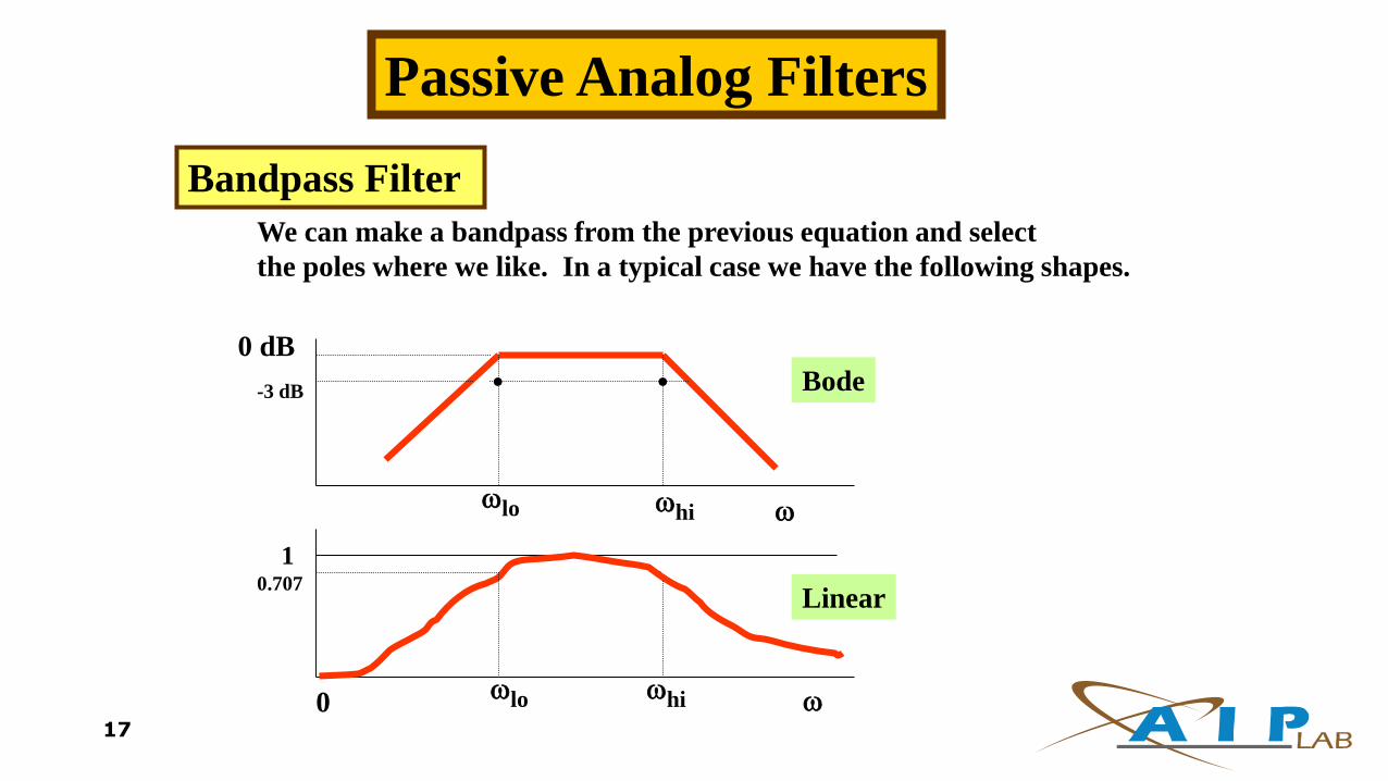
Passive Analog Filters
Bandpass Filter
We can make a bandpass from the previous equation and select
the poles where we like. In a typical case we have the following shapes.
0
0 dB
-3 dB
lo
hi
.
. .
.10.707
Bode
Linear
lo
hi
17
Passive Analog Filters
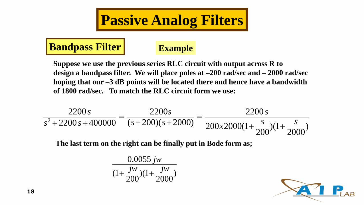
Bandpass Filter Example
Suppose we use the previous series RLC circuit with output across R to
design a bandpass filter. We will place poles at –200 rad/sec and – 2000 rad/sec
hoping that our –3 dB points will be located there and hence have a bandwidth
of 1800 rad/sec. To match the RLC circuit form we use:
2
2200 2200 2200
( 200)( 2000)2200 400000 200 2000(1 )(1 )200 2000
s s ss ss ss s x
The last term on the right can be finally put in Bode form as;
0.0055
(1 )(1 )200 2000
jwjw jw
18

Passive Analog Filters
Bandpass Filter Example
From this last expression we notice from the part involving the zero we
have in dB form;
20log(.0055) + 20logw
Evaluating at w = 200, the first pole break, we get a 0.828 dB
what this means is that our –3dB point will not be at 200 because
we do not have 0 dB at 200. If we could lower the gain by 0.829 dB
we would have – 3dB at 200 but with the RLC circuit we are stuck
with what we have. What this means is that the – 3 dB point will
be at a lower frequency. We can calculate this from
200log 20 0.828
low
dBx dB
w dec
19
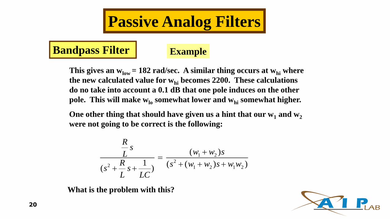
Passive Analog Filters
Bandpass Filter Example
This gives an wlow = 182 rad/sec. A similar thing occurs at whi where
the new calculated value for whi becomes 2200. These calculations
do no take into account a 0.1 dB that one pole induces on the other
pole. This will make wlo somewhat lower and whi somewhat higher.
One other thing that should have given us a hint that our w1 and w2
were not going to be correct is the following:
1 2
22 1 2 1 2
( )
1 ( ( ) )( )
Rs
w w sLR s w w s w w
s sL LC
What is the problem with this?
20

Passive Analog Filters
Bandpass Filter Example
The problem is that we have
1 2 2 1( )R
w w BW w wL
Therein lies the problem. Obviously the above cannot be true and that
is why we have aproblem at the –3 dB points.
We can write a Matlab program and actually check all of this.
We will expect that w1 will be lower than 200 rad/sec and w2 will be
higher than 2000 rad/sec.
21
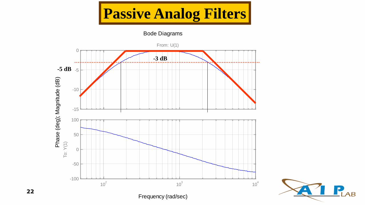
Frequency (rad/sec)
Pha
se
(d
eg
); M
ag
nitud
e (
dB
)
Bode Diagrams
-15
-10
-5
0From: U(1)
102
103
104
-100
-50
0
50
100
To:
Y(1
)
-3 dB
-5 dB
Passive Analog Filters
22

A Bandpass Digital Filter
Perhaps going in the direction to stimulate your interest in taking a course
on filtering, a 10 order analog bandpass butterworth filter will be
simulated using Matlab. The program is given below.
N = 10; %10th order butterworth analog prototype
[ZB, PB, KB] = buttap(N);
numzb = poly([ZB]);
denpb = poly([PB]);
wo = 600; bw = 200; % wo is the center freq
% bw is the bandwidth
[numbbs,denbbs] = lp2bs(numzb,denpb,wo,bw);
w = 1:1:1200;
Hbbs = freqs(numbbs,denbbs,w);
Hb = abs(Hbbs);
plot(w,Hb)
grid
xlabel('Amplitude')
ylabel('frequency (rad/sec)')
title('10th order Butterworth filter')
23

A Bandpass Filter
24
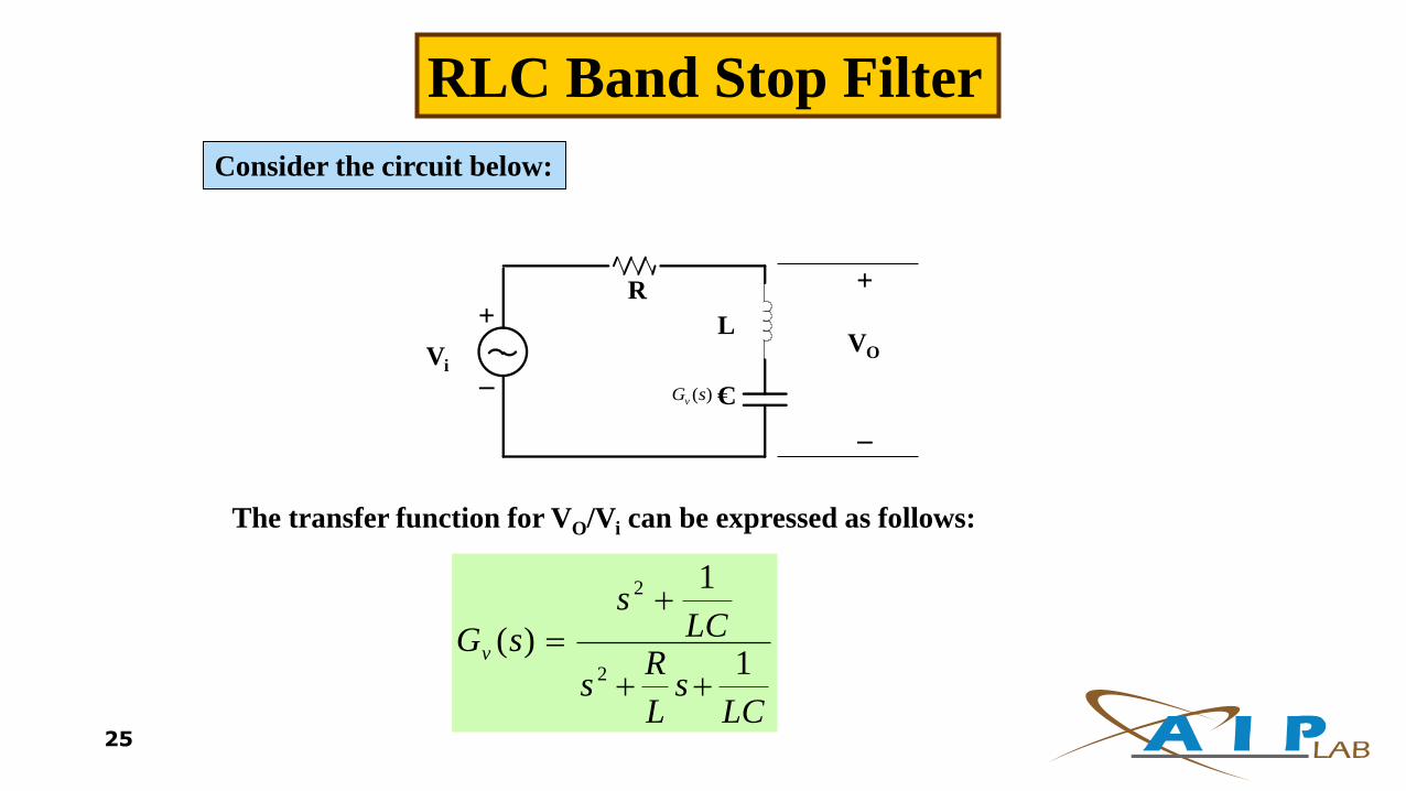
RLC Band Stop Filter
Consider the circuit below:
R
L
C
+
_
VO
+
_Vi
The transfer function for VO/Vi can be expressed as follows:
)(sGv
LCs
L
Rs
LCs
sGv 1
1
)(2
2
25
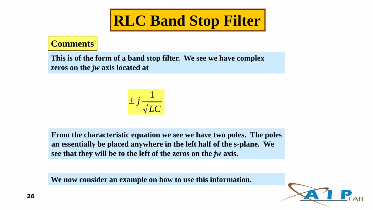
This is of the form of a band stop filter. We see we have complex
zeros on the jw axis located at
RLC Band Stop Filter
Comments
LCj
1
From the characteristic equation we see we have two poles. The poles
an essentially be placed anywhere in the left half of the s-plane. We
see that they will be to the left of the zeros on the jw axis.
We now consider an example on how to use this information.
26
RLC Band Stop Filter
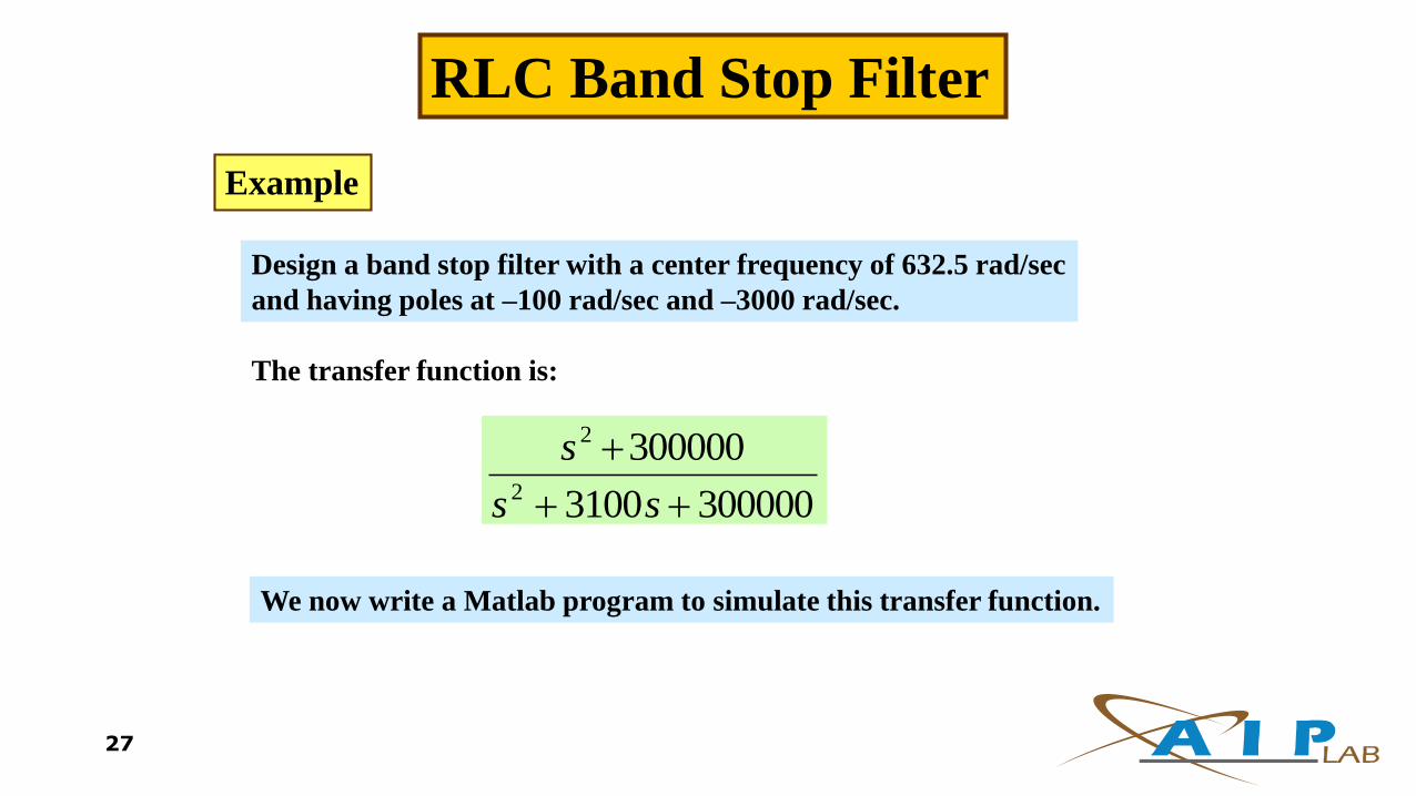
Example
Design a band stop filter with a center frequency of 632.5 rad/sec
and having poles at –100 rad/sec and –3000 rad/sec.
The transfer function is:
3000003100
3000002
2
ss
s
We now write a Matlab program to simulate this transfer function.
27

RLC Band Stop Filter
Example
num = [1 0 300000];
den = [1 3100 300000];
w = 1 : 5 : 10000;
Bode(num,den,w)
28
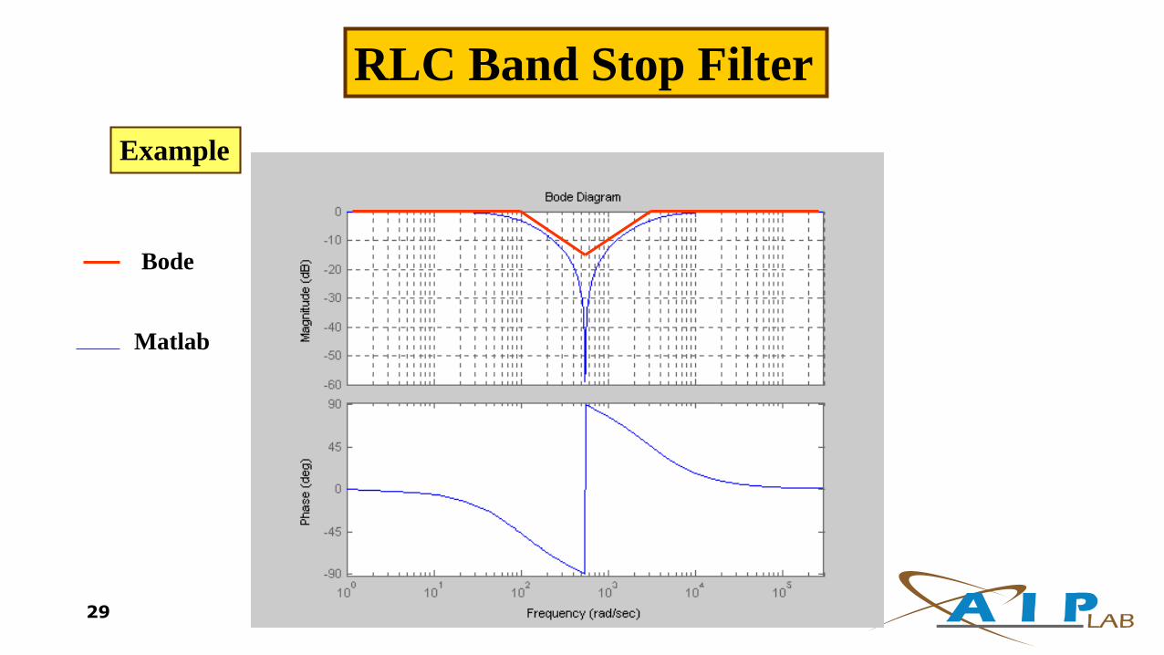
RLC Band Stop Filter
Example
Bode
Matlab
29

VinVO
C
Rfb
+
_
+
_
Rin
Basic Active Filters
Low pass filter
30
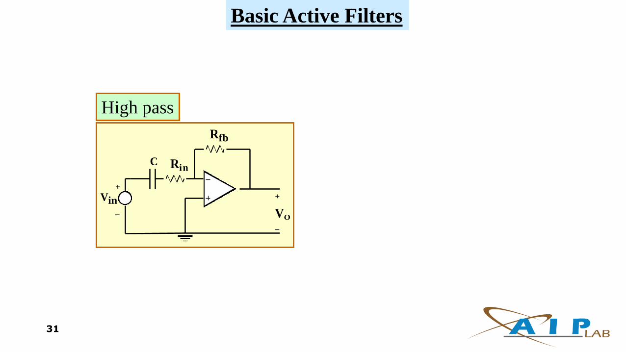
Basic Active Filters
RinC
Vin
Rfb
VO
+
_
+
_
High pass
31
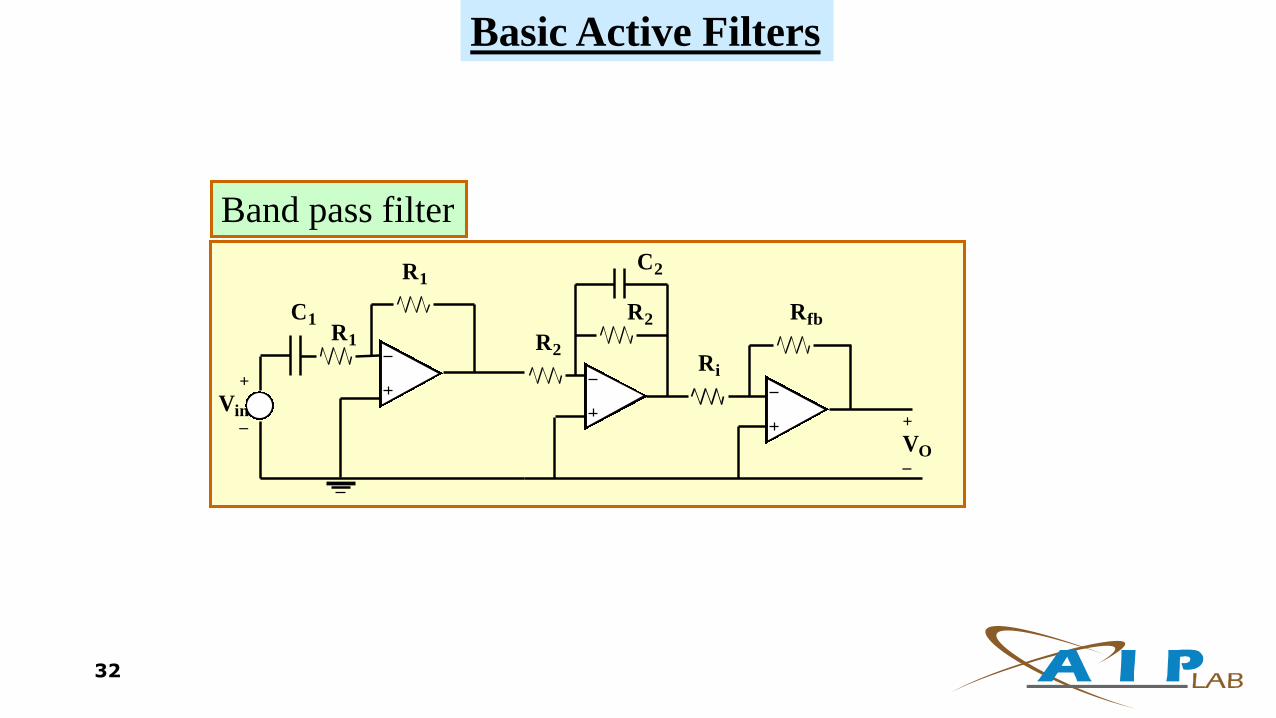
Basic Active Filters
Vin
R1
R1
C1
C2
R2
R2
Rfb
Ri
VO
+
+
_
_
Band pass filter
32
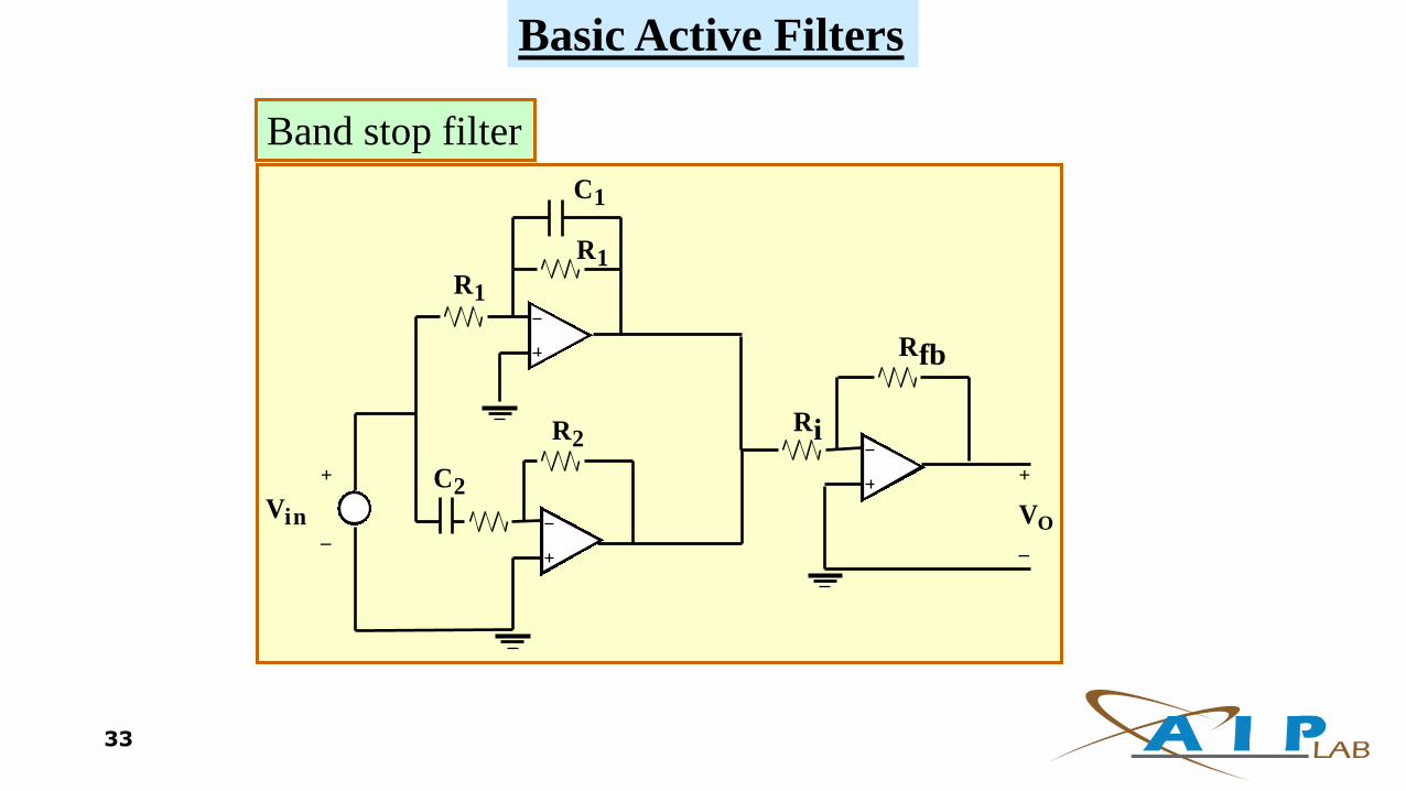
Basic Active Filters
Vin
R1
R1
C1
C2
R2Ri
Rfb
VO
+
_
+
_
Band stop filter
33

ANALOG FILTERS
34

Filters
A filter is a system that processes a signal in some desired fashion.
A continuous-time signal or continuous signal of x(t) is a function of the continuous variable t. A continuous-time signal is often called an analog signal.
A discrete-time signal or discrete signal x(kT) is defined only at discrete instances t=kT, where k is an integer and T is the uniform sampling spacing or period between samples
35
Types of Filters
There are two broad categories of filters:
An analog filter processes continuous-time signals
A digital filter processes discrete-time signals.
The analog or digital filters can be subdivided into four categories:
Lowpass Filters
Highpass Filters
Bandstop Filters
Bandpass Filters36
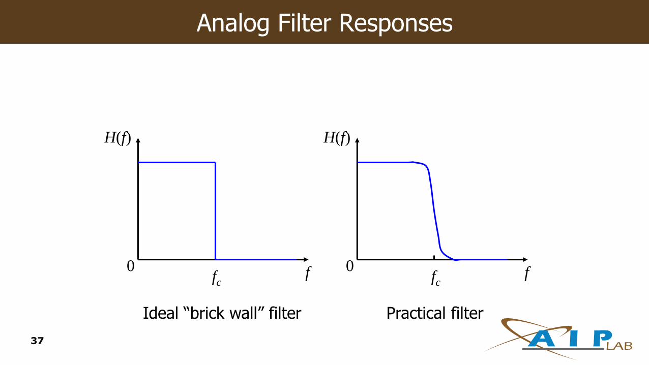
Analog Filter Responses
H(f)
ffc
0
H(f)
ffc
0
Ideal “brick wall” filter Practical filter
37
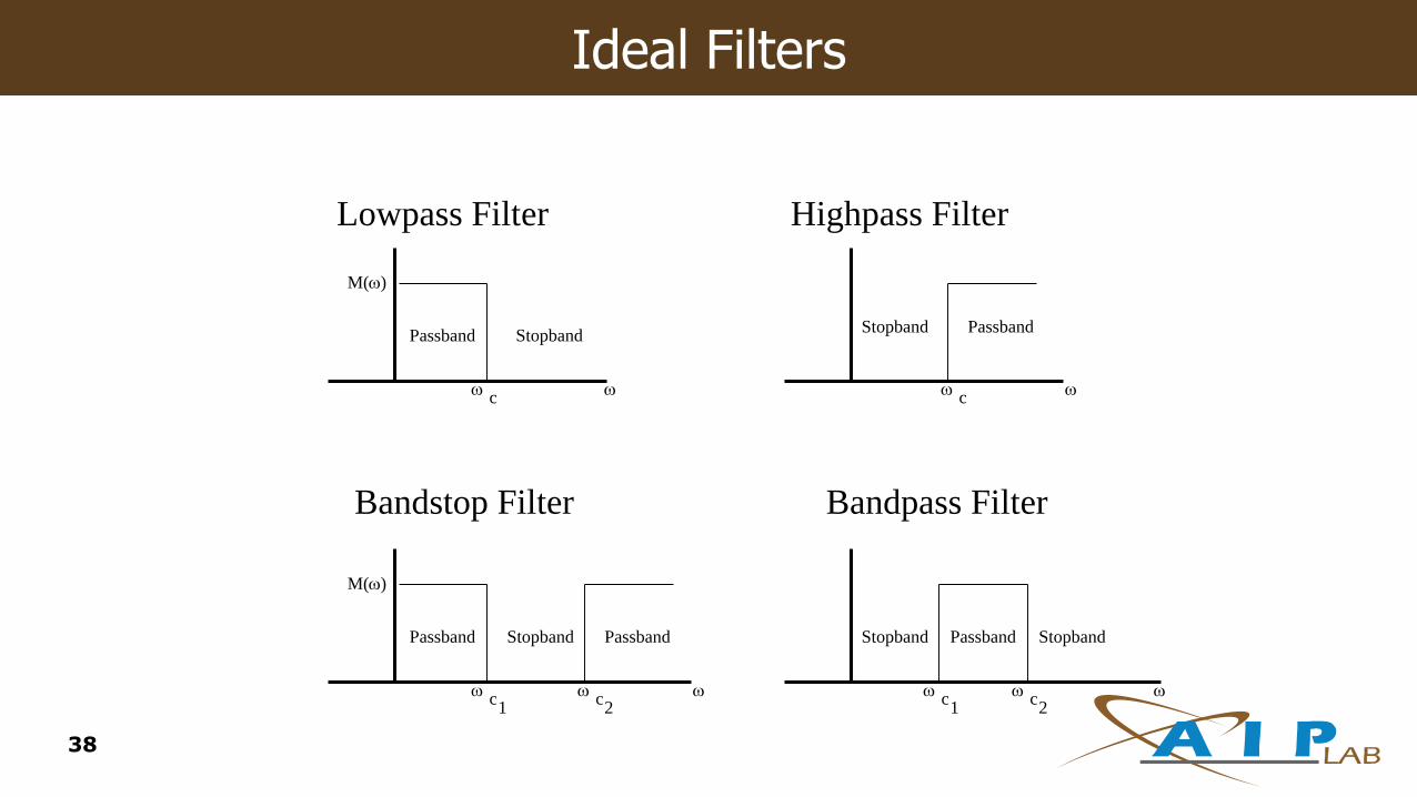
Ideal Filters
Passband StopbandStopband Passband
Passband PassbandStopband
Lowpass Filter Highpass Filter
Bandstop Filter
PassbandStopband Stopband
Bandpass Filter
M()
M()
c
c
c1
c1
c2
c2
38

Passive Filters
Passive filters use resistors, capacitors, and inductors (RLC networks).
To minimize distortion in the filter characteristic, it is desirable to use inductors with high quality factors (remember the model of a practical inductor includes a series resistance), however these are difficult to implement at frequencies below 1 kHz.
They are particularly non-ideal (lossy)
They are bulky and expensive39
Active Filters
Active filters overcome these drawbacks and are realized using resistors, capacitors, and active devices (usually op-amps) which can all be integrated:
Active filters replace inductors using op-amp based equivalent circuits.
40

Op Amp Advantages
Advantages of active RC filters include:reduced size and weight, and therefore parasitics
increased reliability and improved performance
simpler design than for passive filters and can realize a wider range of functions as well as providing voltage gain
in large quantities, the cost of an IC is less than its passive counterpart
41
Op Amp Disadvantages
Active RC filters also have some disadvantages:limited bandwidth of active devices limits the highest attainable pole frequency and therefore applications above 100 kHz (passive RLC filters can be used up to 500 MHz)the achievable quality factor is also limitedrequire power supplies (unlike passive filters)increased sensitivity to variations in circuit parameters caused by environmental changes compared to passive filters
For many applications, particularly in voice and data communications, the economic and performance advantages of active RC filters far outweigh their disadvantages.
42
Bode Plots
Bode plots are important when considering the frequency response characteristics of amplifiers. They plot the magnitude or phase of a transfer function in dB versus frequency.
43

The decibel (dB)
Two levels of power can be compared using a
unit of measure called the bel.
The decibel is defined as:
1 bel = 10 decibels (dB)
1
210log
P
PB
44

Half Power Point
A common dB term is the half power point
which is the dB value when the P2 is one-
half P1.
1
210log10
P
PdB
dBdB 301.32
1log10 10
45

Logarithms
A logarithm is a linear transformation used to
simplify mathematical and graphical operations.
A logarithm is a one-to-one correspondence.
46

Base Number Representation
Any number (N) can be represented as a
base number (b) raised to a power (x).
The value power (x) can be determined by
taking the logarithm of the number (N) to
base (b).
xbN )(
Nx blog
47

Change of Base Logarithm
Although there is no limitation on the numerical value of the base, calculators are designed to handle either base 10 (the common logarithm) or base e (the natural logarithm).
Any base can be found in terms of the common logarithm by:
wq
wq 10
10
loglog
1log
48

Properties of Logarithms
The common or natural
logarithm of the number 1 is 0.
The log of any number less
than 1 is a negative number.
The log of the product of two
numbers is the sum of the logs
of the numbers.
The log of the quotient
of two numbers is the
log of the numerator
minus the denominator.
The log a number taken
to a power is equal to the
product of the power and
the log of the number.
49

Poles & Zeros of the Transfer Function
pole—value of s where the denominator goes to zero.
zero—value of s where the numerator goes to zero.
50
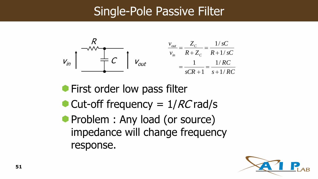
Single-Pole Passive Filter
First order low pass filter
Cut-off frequency = 1/RC rad/s
Problem : Any load (or source) impedance will change frequency response.
vin voutC
R
RCs
RC
sCR
sCR
sC
ZR
Z
v
v
C
C
in
out
/1
/1
1
1
/1
/1
51
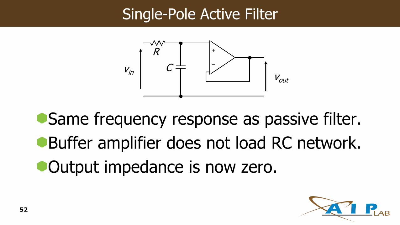
Single-Pole Active Filter
Same frequency response as passive filter.
Buffer amplifier does not load RC network.
Output impedance is now zero.
vinvout
C
R
52

Low-Pass and High-Pass Active Filter Designs
High Pass Low Pass
)/1()/1(
1
1
11
1
RCs
s
RCsRC
sRC
sCR
sRC
sCR
v
v
in
out
RCs
RC
v
v
in
out
/1
/1
53

What are Body plots?
To understand Bode plots, you need to
use Laplace transforms!
The transfer function
of the circuit is:
1
1
/1
/1
)(
)(
sRCsCR
sC
sV
sVA
in
ov
R
Vin(s)
54
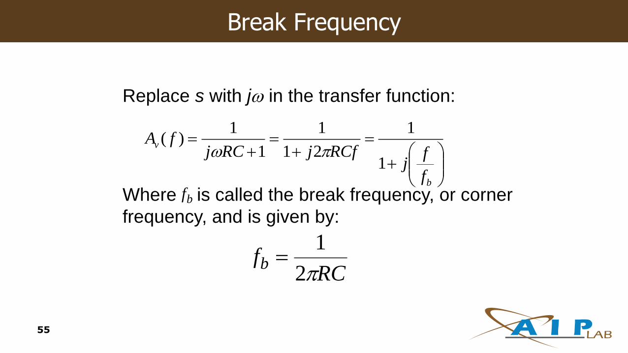
Break Frequency
Replace s with j in the transfer function:
Where is called the break frequency, or corner
frequency, and is given by:
b
v
f
fj
RCfjRCjfA
1
1
21
1
1
1)(
RCfb
2
1
bf
55
Corner Frequency
The significance of the break frequency is that it represents the frequency where
Av(f) = 0.707-45.
This is where the output of the transfer function has an amplitude 3-dB below the input amplitude, and the output phase is shifted by -45 relative to the input.
Therefore, is also known as the 3-dB frequency or the corner frequency.
bf
56
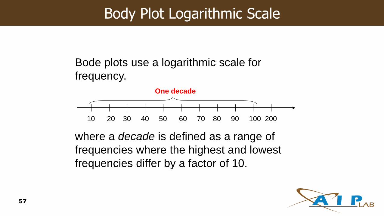
Body Plot Logarithmic Scale
Bode plots use a logarithmic scale for
frequency.
where a decade is defined as a range of
frequencies where the highest and lowest
frequencies differ by a factor of 10.
10 20 30 40 50 60 70 80 90 100 200
One decade
57

Gain or Magnitude of the Transfer Function
Consider the magnitude of the transfer function:
Expressed in dB, the expression is
2/1
1)(
b
v
fffA
b
bb
bdBv
ff
ffff
fffA
/log20
/1log10/1log20
/1log201log20)(
22
2
58
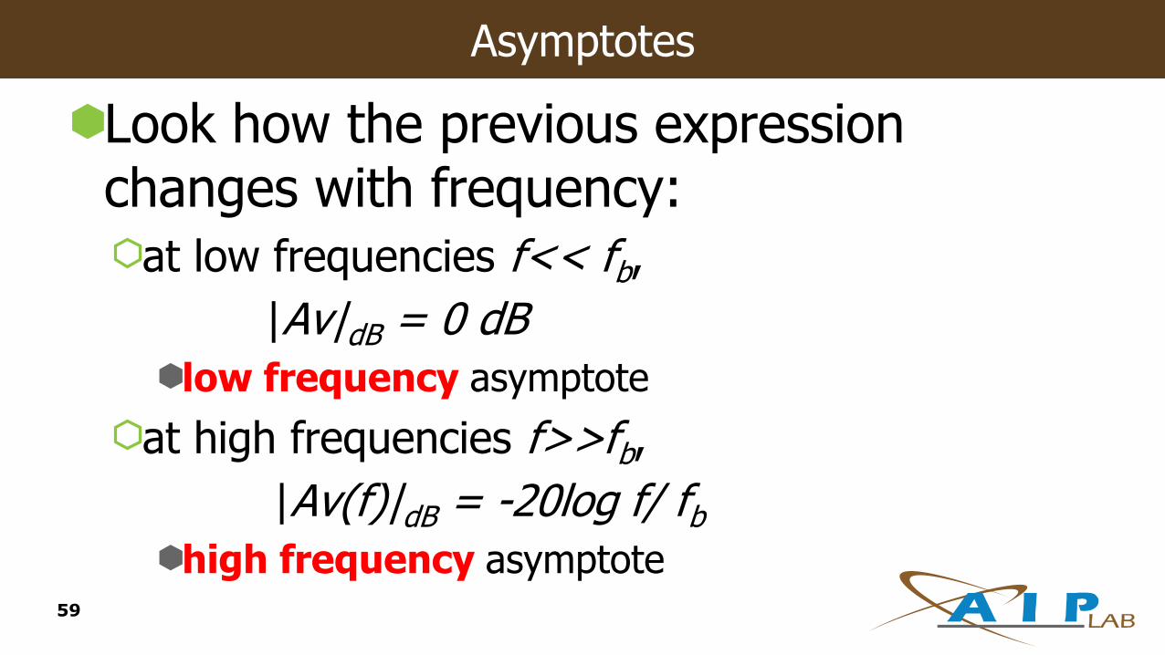
Asymptotes
Look how the previous expression changes with frequency:
at low frequencies f<< fb,
|Av|dB = 0 dB
low frequency asymptote
at high frequencies f>>fb,
|Av(f)|dB = -20log f/ fbhigh frequency asymptote
59

Magnitude
20 log P ( )( )
rad
sec
0.1 1 10 10060
40
20
0
arg P ( )( )
deg
rad
sec
0.1 1 10 100100
50
0
Actual response curve
High frequency asymptote
3 dB
Low frequency asymptote
Note that the two
asymptotes intersect at fbwhere
|Av(fb )|dB = -20log f/ fb
60
Bode Plot Filter Approximation
The technique for approximating a filter function based on Bode plots is useful for low order, simple filter designs
More complex filter characteristics are more easily approximated by using some well-described rational functions, the roots of which have already been tabulated and are well-known.
61
Real Filters
The approximations to the ideal filter are the:
Butterworth filter
Chebyshev filter
Cauer (Elliptic) filter
Bessel filter
62

Standard Transfer Functions
ButterworthFlat Pass-band.
20n dB per decade roll-off.
ChebyshevPass-band ripple.
Sharper cut-off than Butterworth.
EllipticPass-band and stop-band ripple.
Even sharper cut-off.
BesselLinear phase response – i.e. no signal distortion in pass-band.
63

Magnitude Plots of Standard Transfer Functions
64

65
Types of Filters
Butterworth – flat response in the passband and acceptable roll-off
Chebyshev – steeper roll-off but exhibits passband ripple (making it unsuitable for audio systems)
Bessel – yields a constant propagation delay
Elliptical – much more complicated
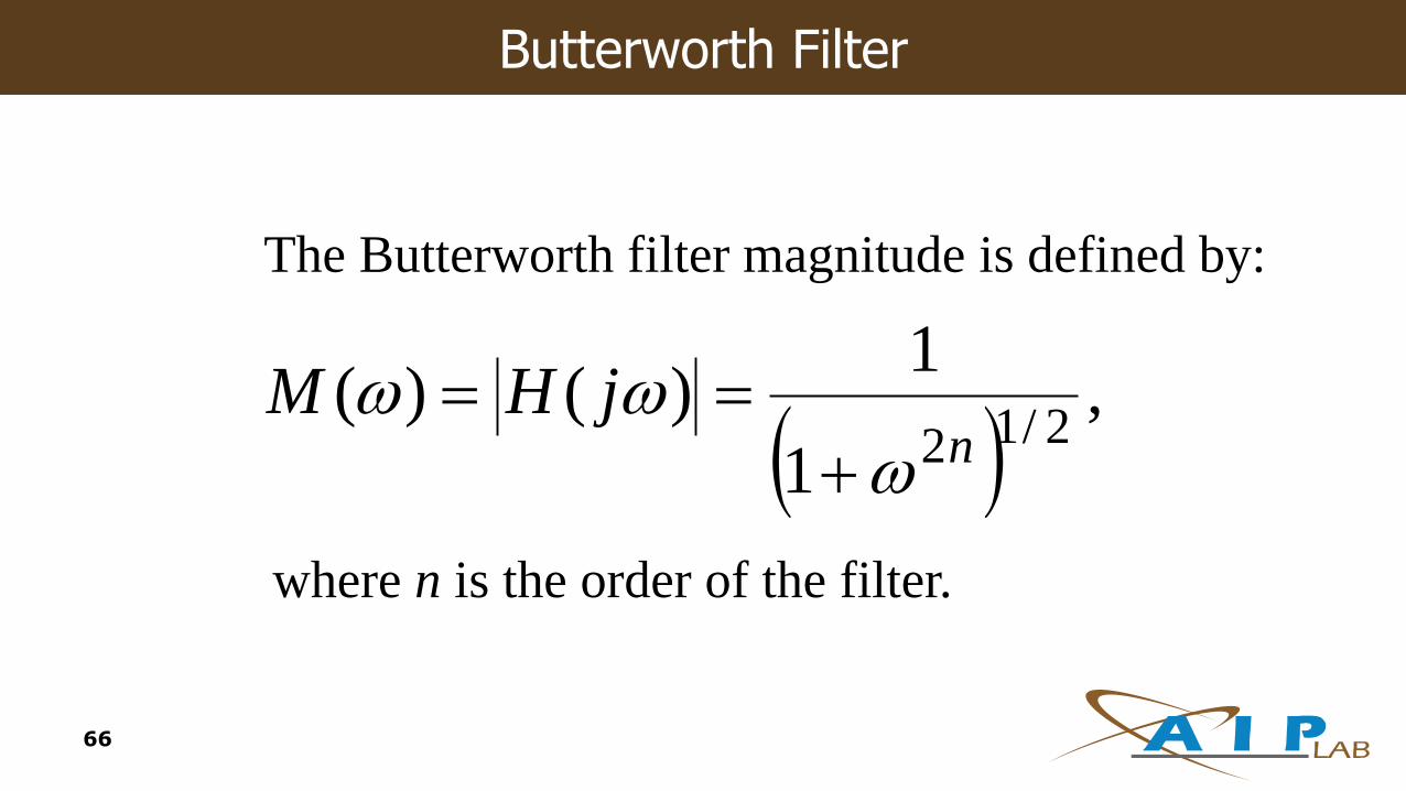
Butterworth Filter
The Butterworth filter magnitude is defined by:
where n is the order of the filter.
,
1
1)()(
2/12njHM
66

Filter Magnitude Approximation
From the previous slide:
for all values of n
For large :
1)0( M
2
1)1( M
nM
1)(
67
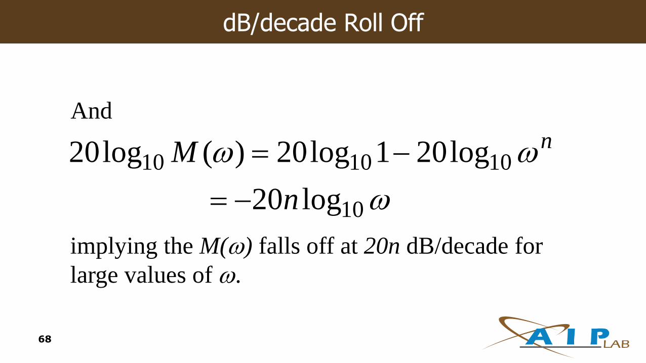
dB/decade Roll Off
And
implying the M() falls off at 20n dB/decade for
large values of .
10
101010
log20
log201log20)(log20
n
M n
68

dB/decade Roll Off Examples
T1i
T2i
T3i
wi
1000
0.1 1 100.01
0.1
1
10
20 db/decade
40 db/decade
60 db/decade
69
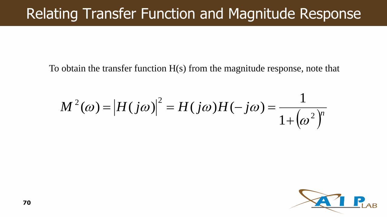
Relating Transfer Function and Magnitude Response
To obtain the transfer function H(s) from the magnitude response, note that
njHjHjHM
2
22
1
1)()()()(
70

Complex Conjugation and Frequency Response
Because s j for the frequency response, we have s2 2.
The poles of this function are given by the roots of
nnnss
sHsH22 11
1
1
1)()(
nkes kjnn2,,2,1,111 )12(2
71
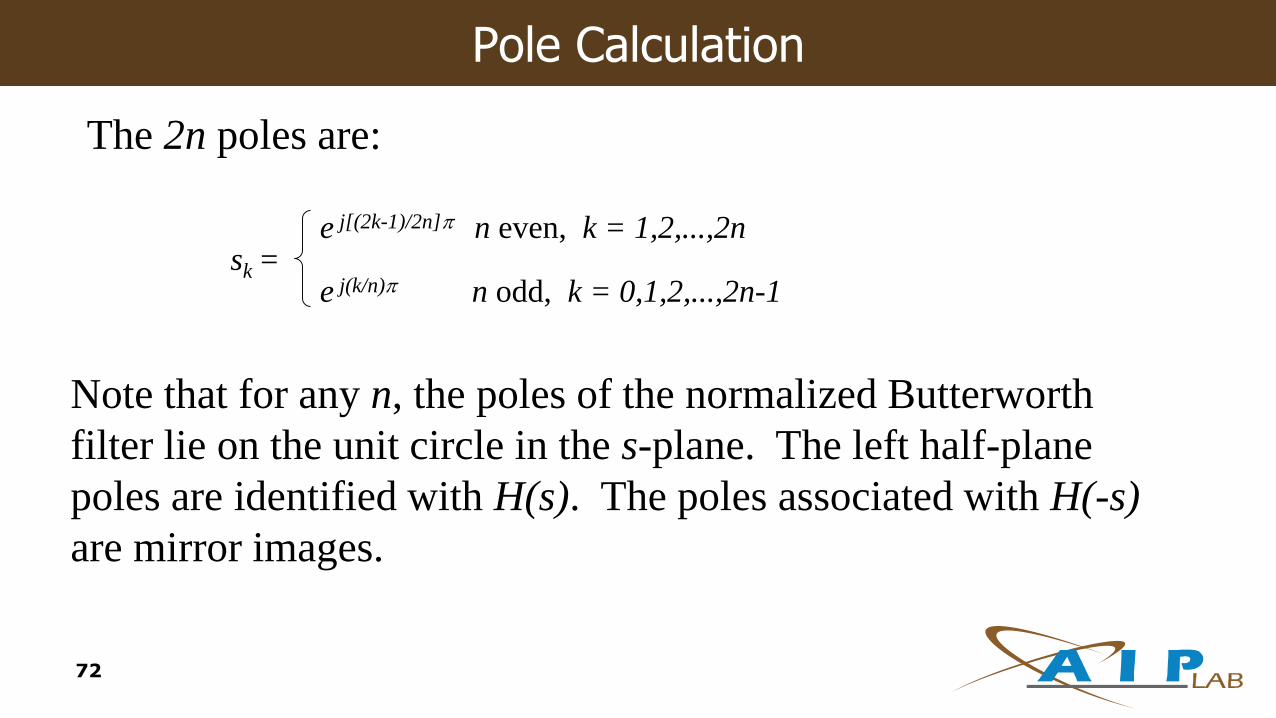
Pole Calculation
The 2n poles are:
sk =e j[(2k-1)/2n] n even, k = 1,2,...,2n
e j(k/n) n odd, k = 0,1,2,...,2n-1
Note that for any n, the poles of the normalized Butterworth
filter lie on the unit circle in the s-plane. The left half-plane
poles are identified with H(s). The poles associated with H(-s)
are mirror images.
72

S-Plane Pole Placement
73
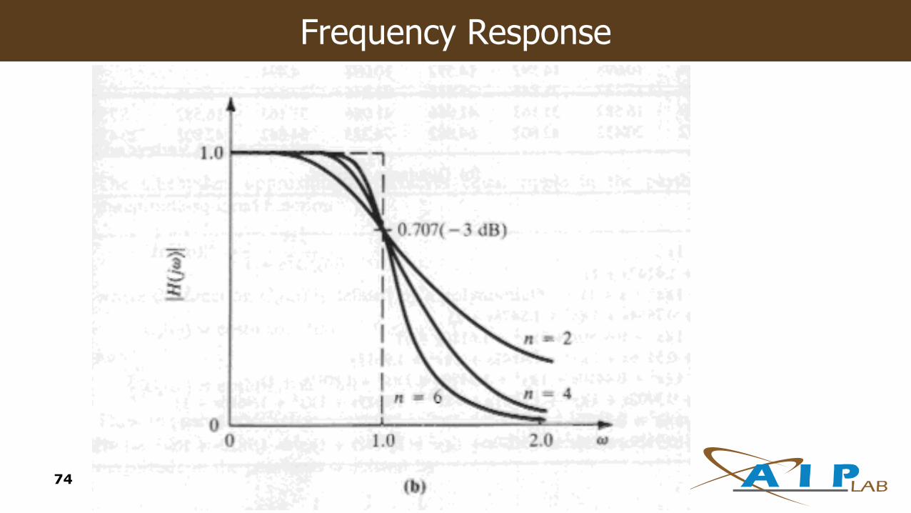
Frequency Response
74

Phasor’s Rectangular and Polar Representations
Recall from complex numbers that the rectangular form
of a complex can be represented as:
Recalling that the previous equation is a phasor, we can
represent the previous equation in polar form:
jyxz
sincos jrz where
sincos ryandrx
75
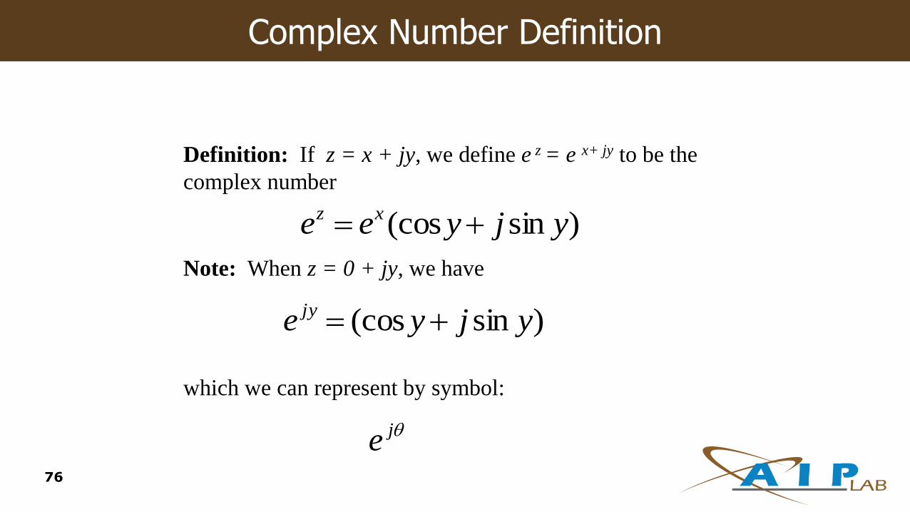
Complex Number Definition
Definition: If z = x + jy, we define e z = e x+ jy to be the
complex number
Note: When z = 0 + jy, we have
which we can represent by symbol:
e j
)sin(cos yjyee xz
)sin(cos yjye jy
76

Euler’s Law
)sin(cos je j
The following equation is known as Euler’s law.
Note that
functionodd
functioneven
sinsin
coscos
77
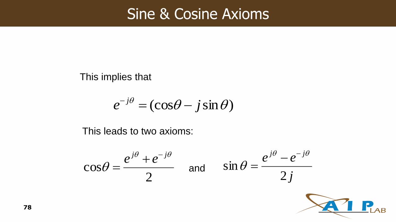
Sine & Cosine Axioms
)sin(cos je j
This implies that
This leads to two axioms:
2cos
jj ee
andj
ee jj
2sin
78

Complex Unit Vector
Observe that e j represents a unit vector which makes an angle with the positive x axis.
79
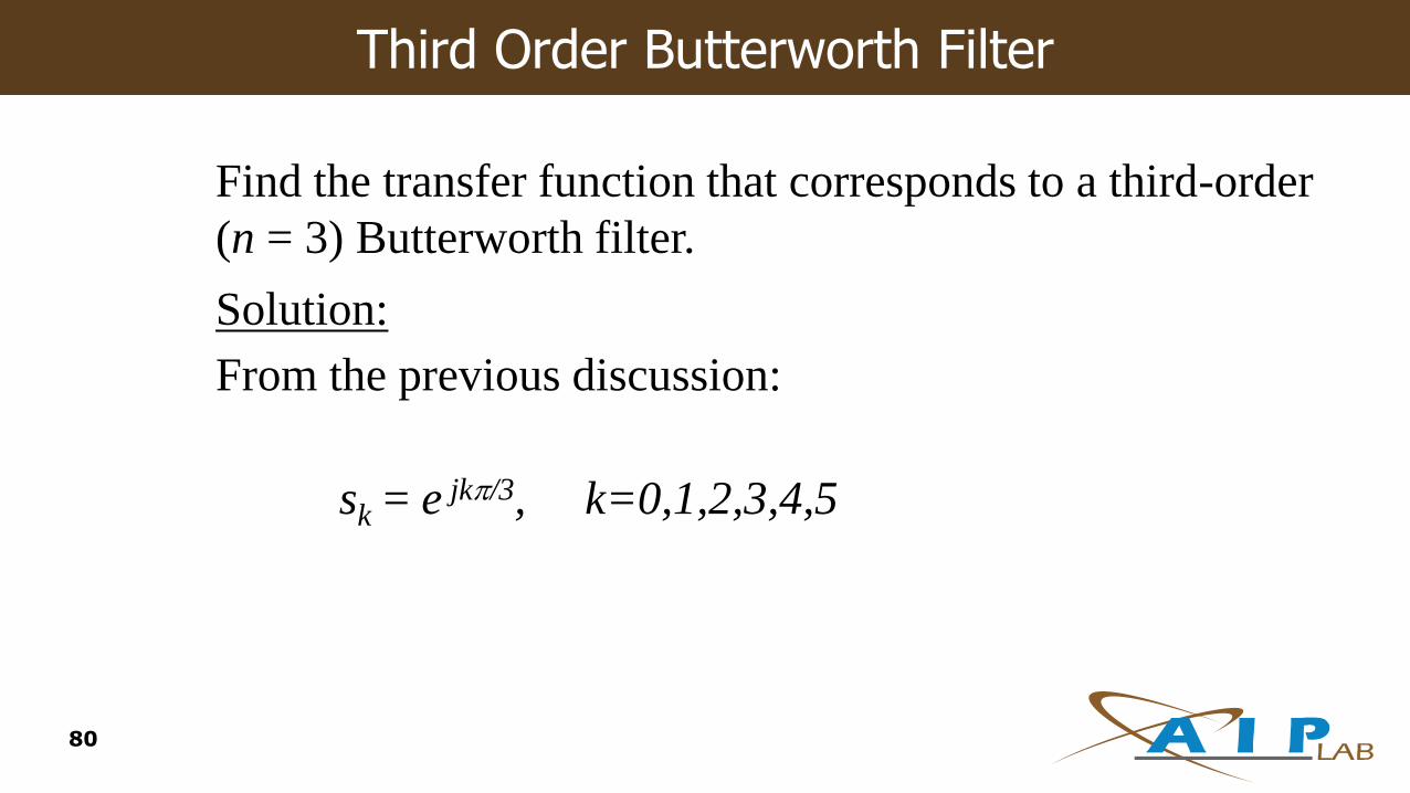
Third Order Butterworth Filter
Find the transfer function that corresponds to a third-order
(n = 3) Butterworth filter.
Solution:
From the previous discussion:
sk = e jk/3, k=0,1,2,3,4,5
80
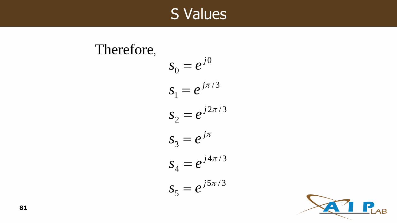
S Values
Therefore,
3/5
5
3/4
4
3
3/2
2
3/
1
0
0
j
j
j
j
j
j
es
es
es
es
es
es
81
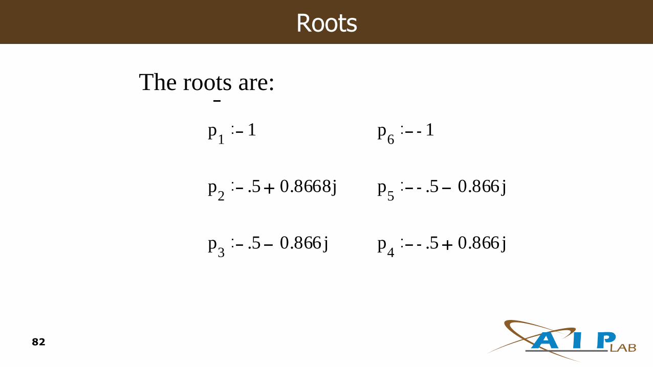
Roots
p1
1 p6
1
p2
.5 0.8668j p5
.5 0.866j
p3
.5 0.866 j p4
.5 0.866j
The roots are:
82

Filter Design Table
The factored form of the normalized Butterworth polynomials for various order n are tabulated in filter design tables.
83
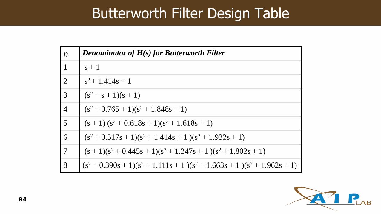
Butterworth Filter Design Table
n Denominator of H(s) for Butterworth Filter
1 s + 1
2 s2 + 1.414s + 1
3 (s2 + s + 1)(s + 1)
4 (s2 + 0.765 + 1)(s2 + 1.848s + 1)
5 (s + 1) (s2 + 0.618s + 1)(s2 + 1.618s + 1)
6 (s2 + 0.517s + 1)(s2 + 1.414s + 1 )(s2 + 1.932s + 1)
7 (s + 1)(s2 + 0.445s + 1)(s2 + 1.247s + 1 )(s2 + 1.802s + 1)
8 (s2 + 0.390s + 1)(s2 + 1.111s + 1 )(s2 + 1.663s + 1 )(s2 + 1.962s + 1)
84

DIGITAL FILTERS
85
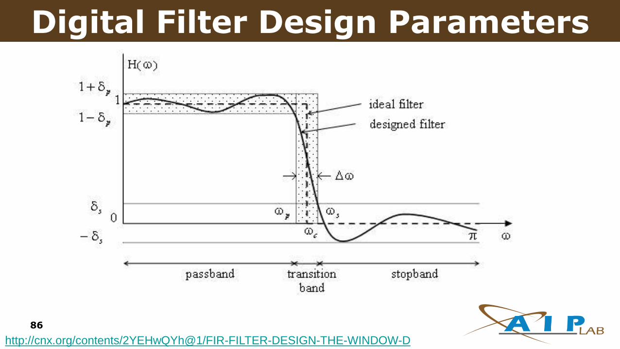
Digital Filter Design Parameters
86
http://cnx.org/contents/2YEHwQYh@1/FIR-FILTER-DESIGN-THE-WINDOW-D
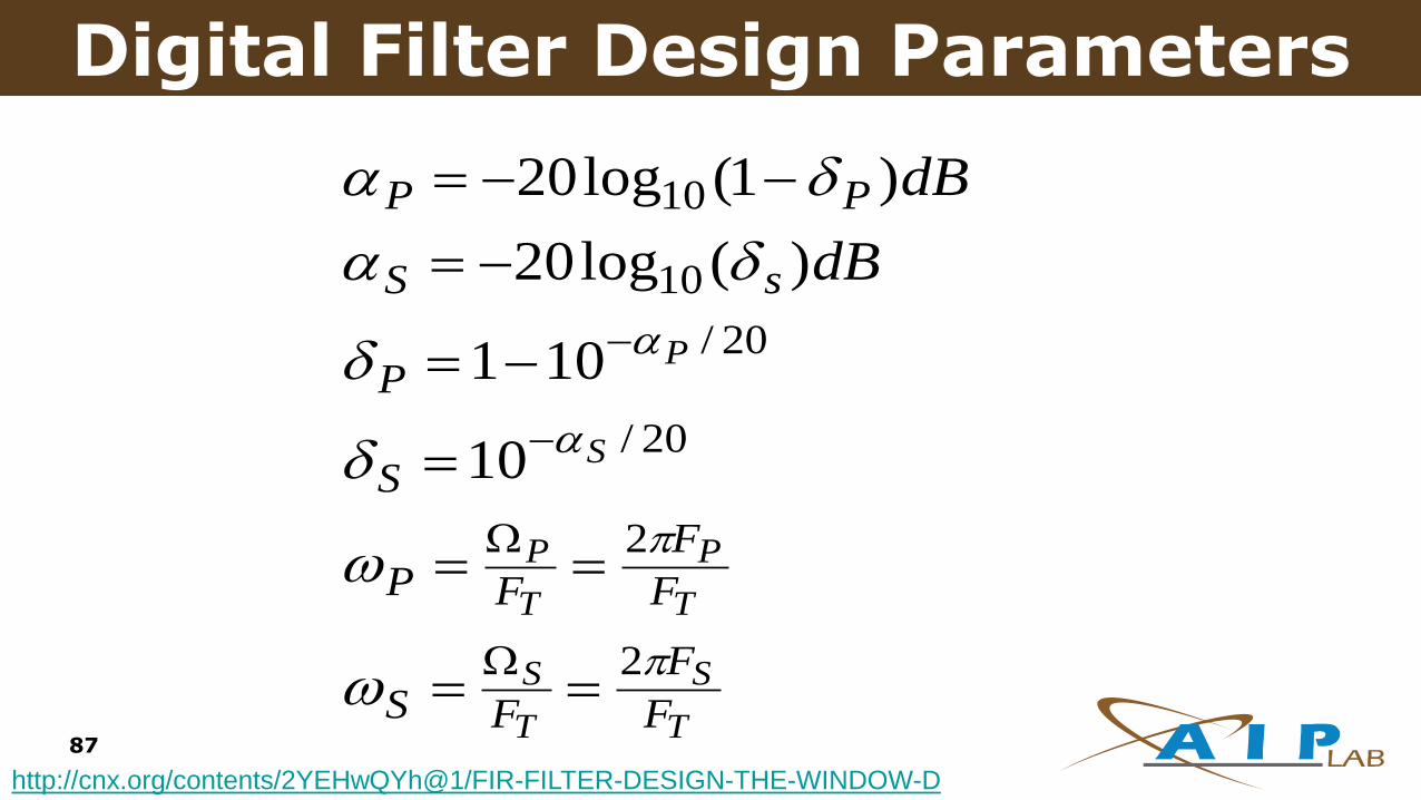
Digital Filter Design Parameters
87
http://cnx.org/contents/2YEHwQYh@1/FIR-FILTER-DESIGN-THE-WINDOW-D
T
S
T
S
T
P
T
P
S
P
F
F
FS
F
F
FP
S
P
sS
PP
dB
dB
2
2
20/
20/
10
10
10
101
)(log20
)1(log20

Analog-Based Digital Filters
88
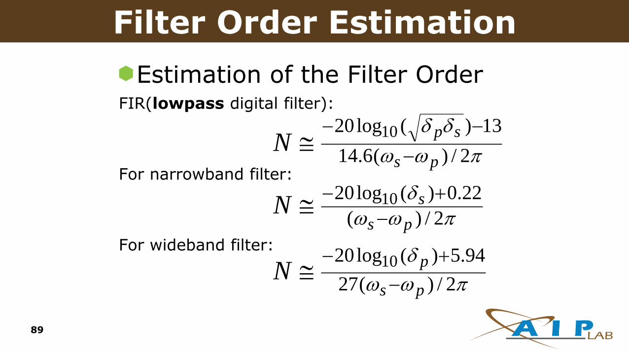
Filter Order Estimation
89
Estimation of the Filter OrderFIR(lowpass digital filter):
For narrowband filter:
For wideband filter:
2/)(27
94.5)(log20
2/)(
22.0)(log20
2/)(6.14
13)(log20
10
10
10
ps
p
ps
s
ps
sp
N
N
N

90
Digital Signal Processing
Filter Design: IIR
1. Filter Design Specifications
2. Analog Filter Design
3. Digital Filters from Analog Prototypes
Filter Order Estimation
91
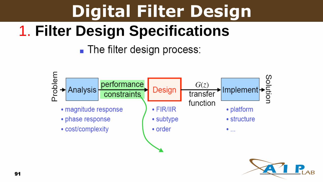
1. Filter Design Specifications
Digital Filter Design
92
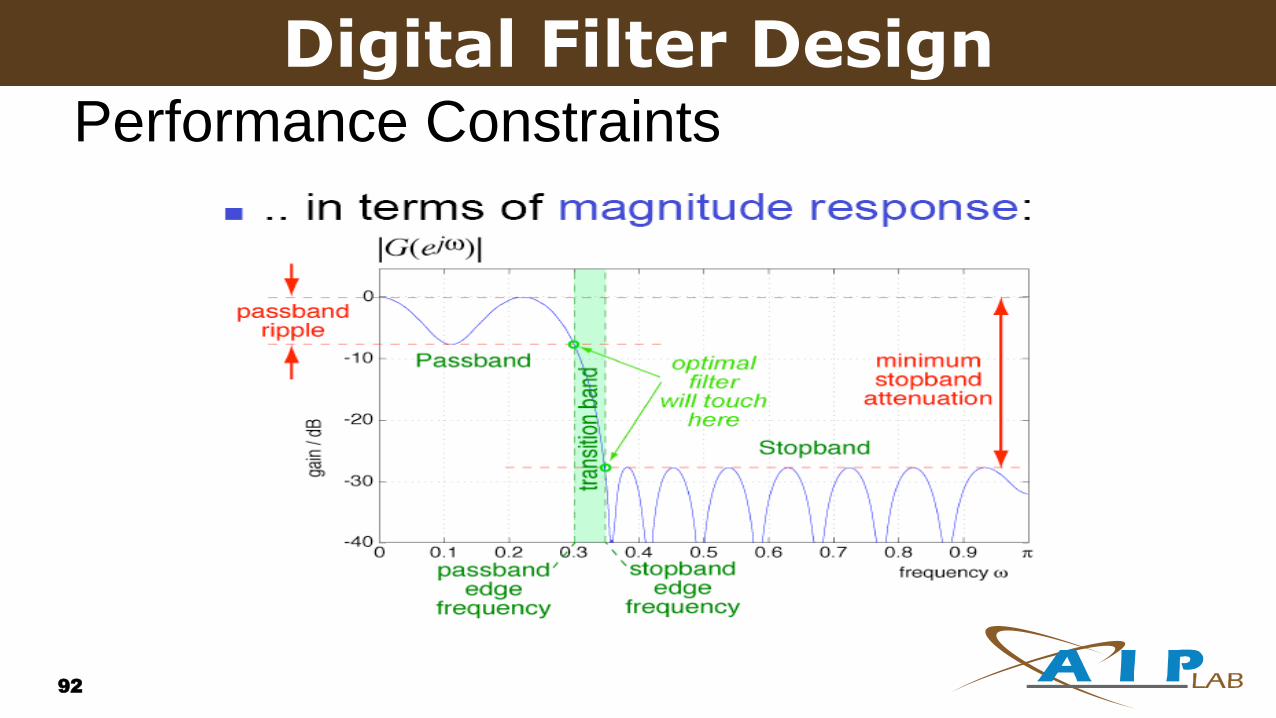
Performance Constraints
Digital Filter Design

93
Performance Constraints
Digital Filter Design
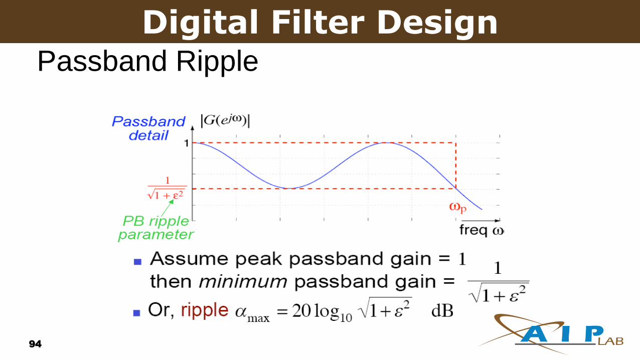
94
Passband Ripple
Digital Filter Design

95
Stopband Ripple
Digital Filter Design

96
Filter Type Choice : FIR vs. IIR
Digital Filter Design

97
FIR vs. IIR
Digital Filter Design
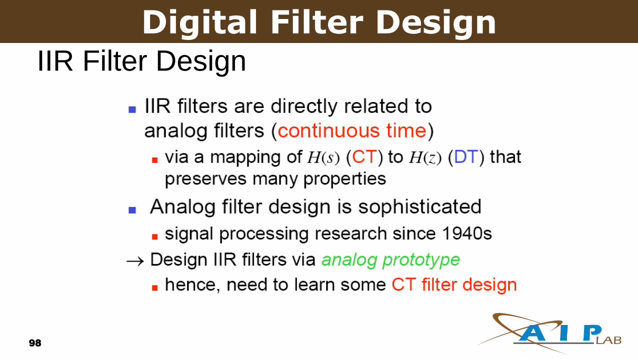
98
IIR Filter Design
Digital Filter Design

99
2. Analog Filter Design
Digital Filter Design
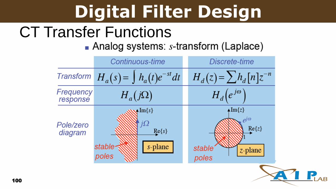
100
CT Transfer Functions
Digital Filter Design
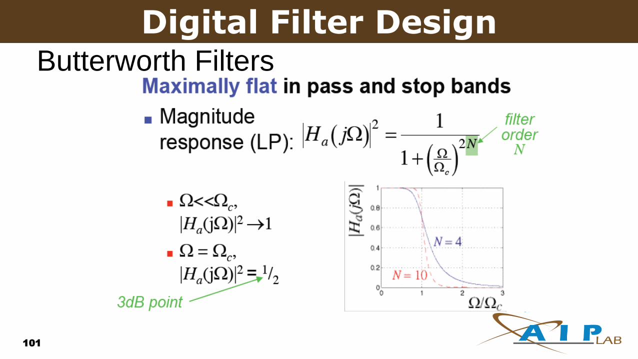
101
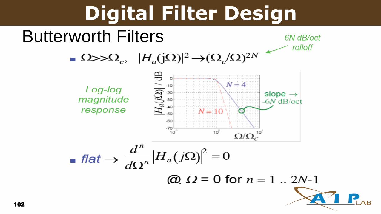
Butterworth Filters
Digital Filter Design
102
Butterworth Filters
Digital Filter Design

103
Digital Filter DesignButterworth Filters

104
Butterworth Filters
Digital Filter Design
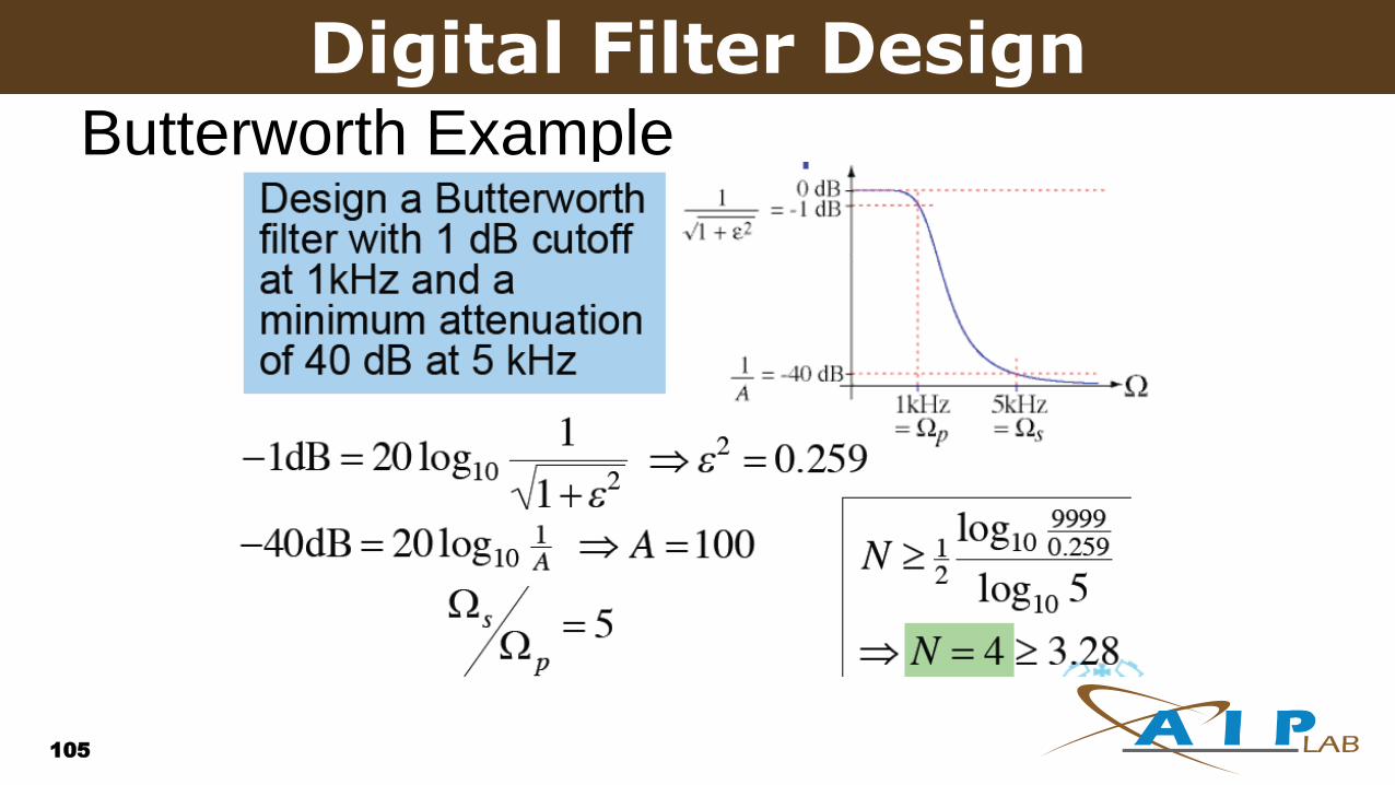
105
Butterworth Example
Digital Filter Design

106
Butterworth Example
Digital Filter Design

107
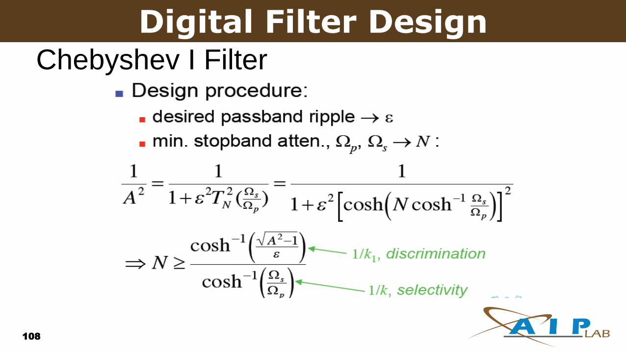
Chebyshev I Filter
Digital Filter Design
108
Chebyshev I Filter
Digital Filter Design

109
Chebyshev I Filter
Digital Filter Design

110
Chebyshev II Filter
Digital Filter Design

111
Elliptical (Cauer) Filters
Digital Filter Design
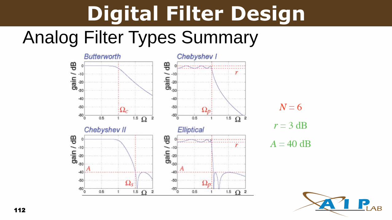
112
Analog Filter Types Summary
Digital Filter Design

FILTER DESIGN
113

MATLAB for Signal Processing
The MathWorks Inc.
Natick, MA
USA
Filter Design
114

Copyright 1984 - 2001 by The MathWorks, Inc.
115MATLAB for Signal Processing
Filter Design
• Frequency selective system
• Analog
• Digital
– Infinite impulse response (IIR)
– Finite impulse response (FIR) a=1
N
k
k
M
m
m knyamnxbny10
)()()(
M
m
m mnxbny0
)()(
Copyright 1984 - 2001 by The MathWorks, Inc.
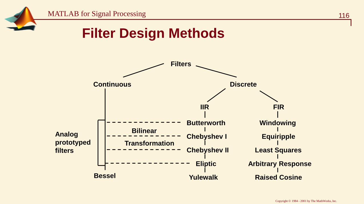
116MATLAB for Signal Processing
Filters
DiscreteContinuous
IIR FIR
Chebyshev I
Chebyshev II
Eliptic
Yulewalk
Butterworth
Arbitrary Response
Equiripple
Least Squares
Raised Cosine
Windowing
Bessel
Analog
prototyped
filters
Bilinear
Transformation
Filter Design Methods

Copyright 1984 - 2001 by The MathWorks, Inc.
117MATLAB for Signal Processing
Transition Band
Stopband
Attenuation
Passband Ripple
Passband Stopband
Fs/2
Filter Specification
• Wp, Ws, Rp, Rs
Copyright 1984 - 2001 by The MathWorks, Inc.
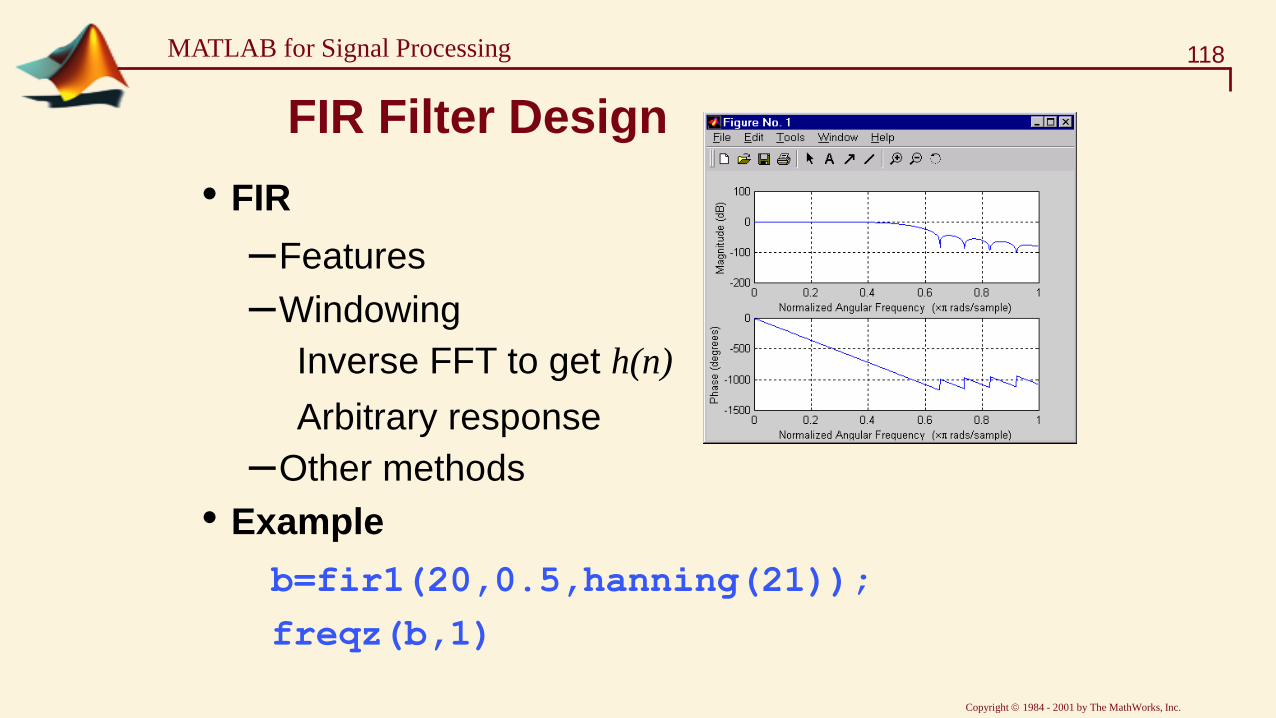
118MATLAB for Signal Processing
FIR Filter Design
• FIR
–Features
–Windowing
Inverse FFT to get h(n)
Arbitrary response
–Other methods
• Example
b=fir1(20,0.5,hanning(21));
freqz(b,1)
Copyright 1984 - 2001 by The MathWorks, Inc.
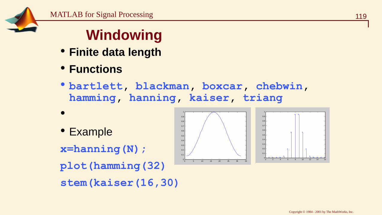
119MATLAB for Signal Processing
Windowing• Finite data length
• Functions
• bartlett, blackman, boxcar, chebwin, hamming, hanning, kaiser, triang
•
• Example
x=hanning(N);
plot(hamming(32)
stem(kaiser(16,30)
0 5 10 15 20 25 30 350
0.1
0.2
0.3
0.4
0.5
0.6
0.7
0.8
0.9
1
0 2 4 6 8 10 12 14 160
0.1
0.2
0.3
0.4
0.5
0.6
0.7
0.8
0.9
1

Copyright 1984 - 2001 by The MathWorks, Inc.
120MATLAB for Signal Processing
Filter Design Tradeoffs
Reduced width of
transition band
FIR
Higher Order
Always Stable
Passband Phase
Linear
IIR
Lower Order
Can be Unstable
Non-linear Phase
Increased complexity
(higher order)
<==>
Lower Rp, Higher Rs Increased complexity
(higher order)
<==>

Copyright 1984 - 2001 by The MathWorks, Inc.
121MATLAB for Signal Processing
Filter Design with FDATool
Import filter
coefficients or
design filter
Set quantization
parameters for
Filter Design
Toolbox
Analysis method for
analyzing filter design
Quantize
current filter
using Filter
Design Toolbox
Filter
specifications
Type of filter to
design and
method to use
»fdatool

Copyright 1984 - 2001 by The MathWorks, Inc.
122MATLAB for Signal Processing
Importing Existing Designs

Copyright 1984 - 2001 by The MathWorks, Inc.
123MATLAB for Signal Processing
Analyze Filters with FDATool

Copyright 1984 - 2001 by The MathWorks, Inc.
124MATLAB for Signal Processing
Print Preview and Annotation

Copyright 1984 - 2001 by The MathWorks, Inc.
125MATLAB for Signal Processing
Convenient Exporting from FDATool

126
Digital Filter Design

127
Starting FDATool
Start MATLAB. At the command line, type in “fdatool”.
The following screen will appear:
128
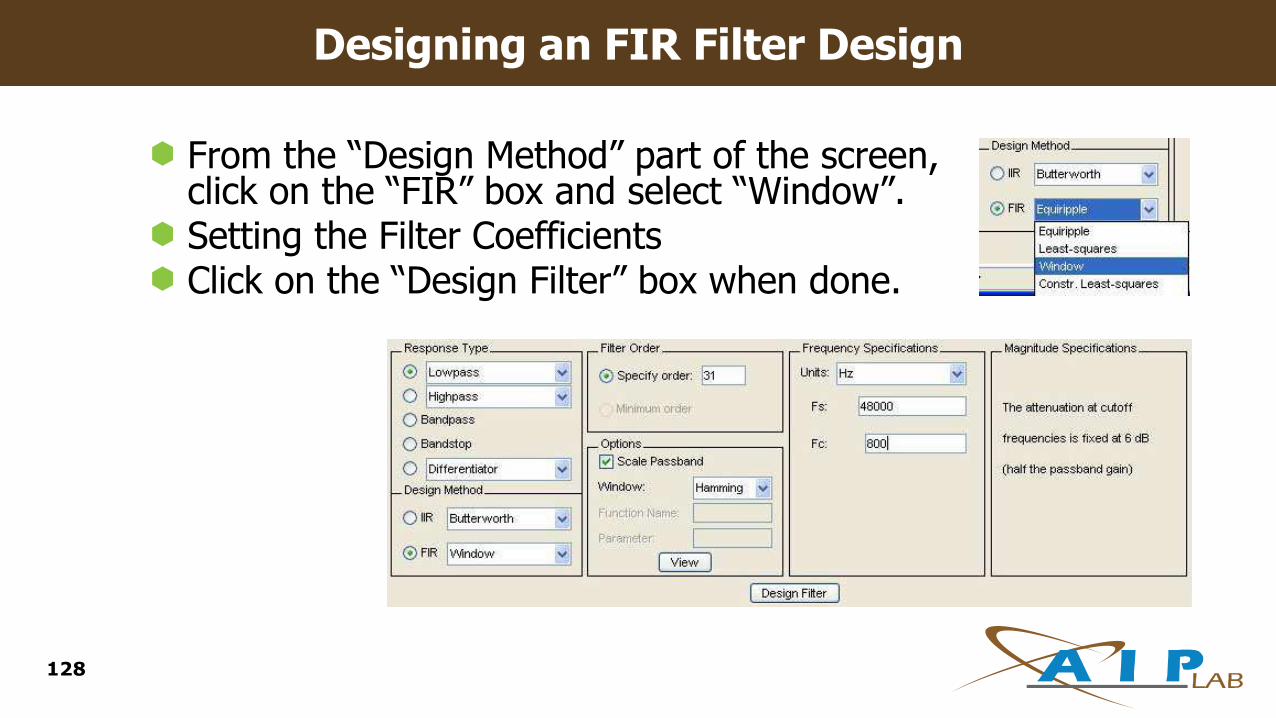
Designing an FIR Filter Design
From the “Design Method” part of the screen, click on the “FIR” box and select “Window”.Setting the Filter CoefficientsClick on the “Design Filter” box when done.
129
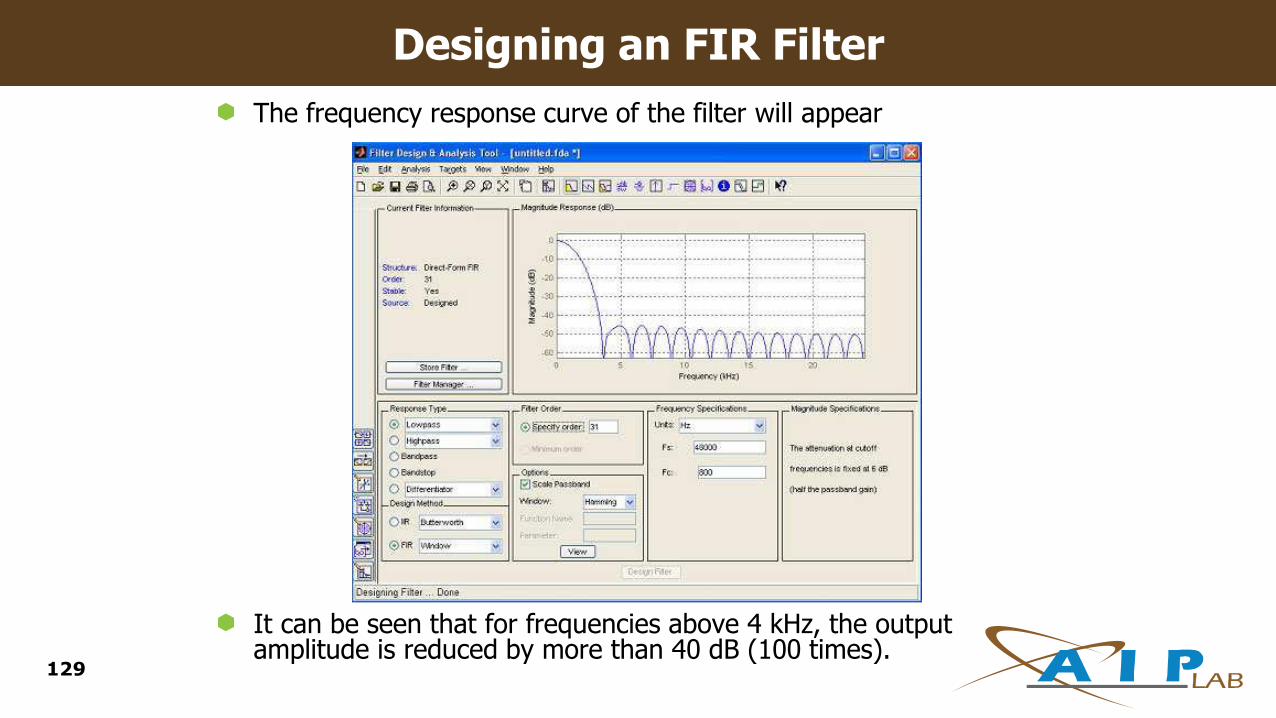
Designing an FIR Filter
The frequency response curve of the filter will appear
It can be seen that for frequencies above 4 kHz, the output amplitude is reduced by more than 40 dB (100 times).
130
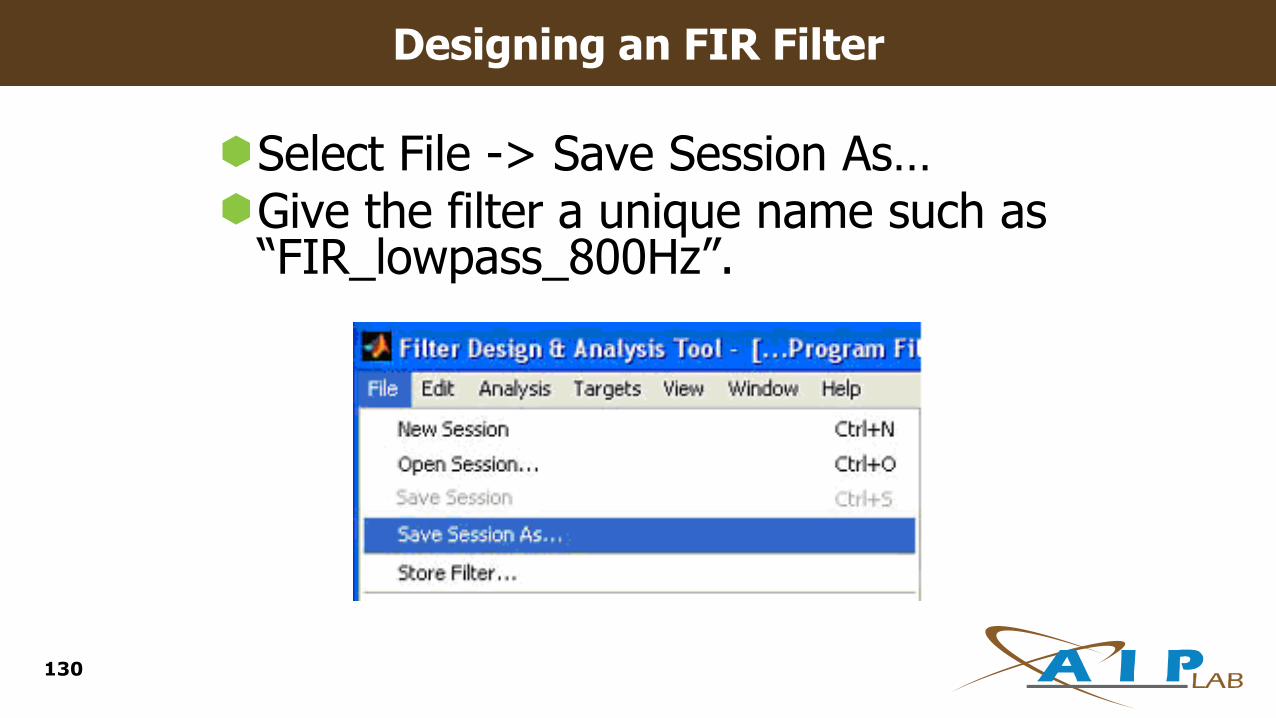
Designing an FIR Filter
Select File -> Save Session As…Give the filter a unique name such as “FIR_lowpass_800Hz”.
131
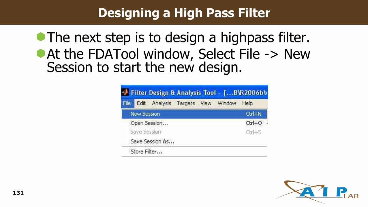
Designing a High Pass Filter
The next step is to design a highpass filter.At the FDATool window, Select File -> New Session to start the new design.

132
The Highpass Filter Design
Set the “Response Type” to “Highpass”.Notice that the “Filter Specifications” part of the screen changes.

133
Entering the Filter Parameters
Click on the “Design Filter” box when done.
134
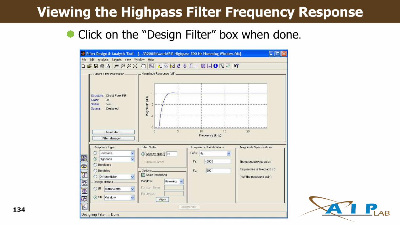
Viewing the Highpass Filter Frequency Response
Click on the “Design Filter” box when done.
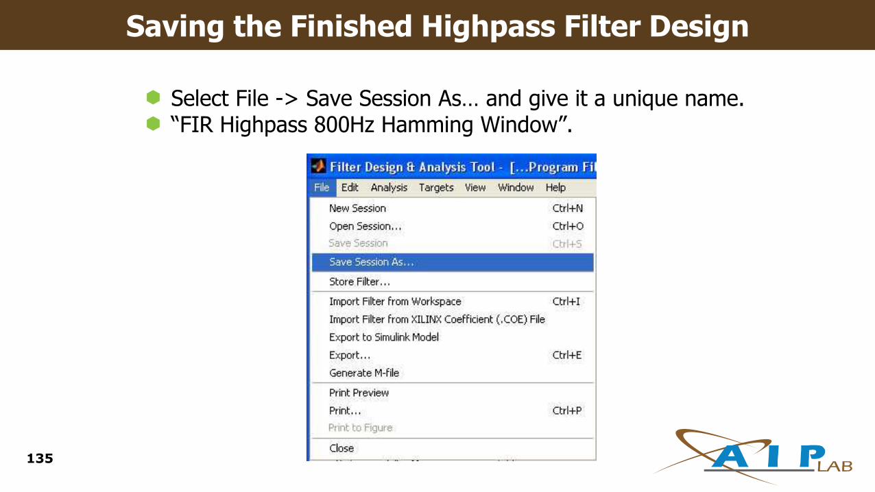
135
Saving the Finished Highpass Filter Design
Select File -> Save Session As… and give it a unique name.“FIR Highpass 800Hz Hamming Window”.

136
PSPICE
What is Spice?
Spice is the short form of:
Simulated
Program with
Integrated
Circuit
Emphasis
137

Why PSPICE Programming?
Don’t have to draw the circuit
More control over the parts
More control over the analysis
Don’t have to search for parts
Some SPICE software applications (HSPICE, etc.) don’t have GUI at all
Quick and efficient138
Steps of PSPICE Programming
Draw the circuit and label the nodes
Create netlist (*.cir) file
Add in control statements
Add in title, comment & end statements
Run PSPICE
Evaluate the results of the output
139

MATLAB and SPICE Features
MATLABSPICEFeatures
small circuitssmall to very large
circuits
Type of Circuit For
Analysis
YesYesFrequency
Response
NoYes
Inclusion of Device
Model in Software
Package
140
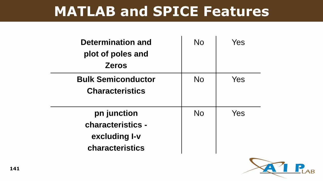
MATLAB and SPICE Features
YesNoDetermination and
plot of poles and
Zeros
YesNoBulk Semiconductor
Characteristics
YesNopn junction
characteristics -
excluding I-v
characteristics
141

142
PHASOR ANALYSIS
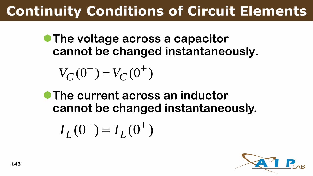
Continuity Conditions of Circuit Elements
The voltage across a capacitor cannot be changed instantaneously.
)0()0( CC VV
)0()0( LL II
The current across an inductor cannot be changed instantaneously.
143
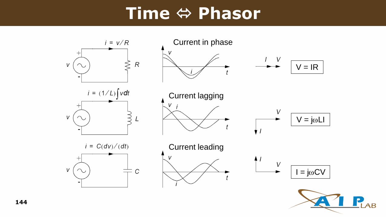
Time Phasor
Current in phase
Current lagging
Current leading
V = IR
V = jLI
I = jCV
144
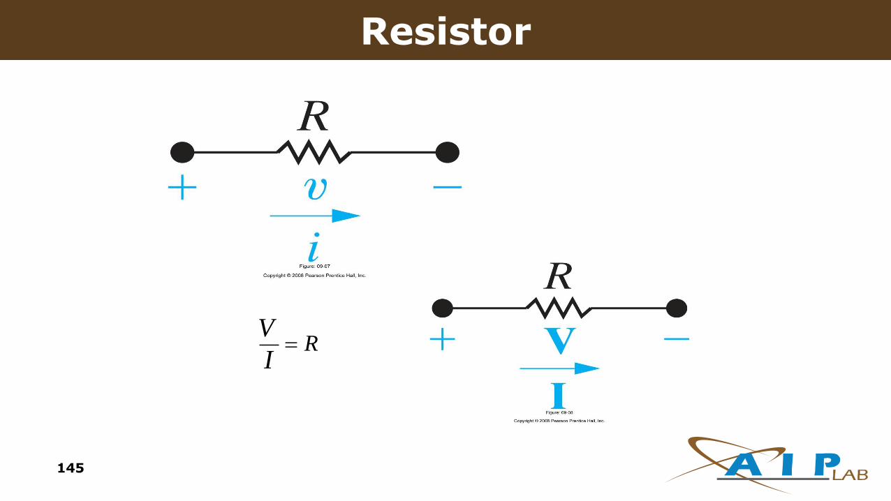
RI
V
Resistor
145

Instantaneous Response
146

LjI
V
Inductor
147

Current Lags Voltage in an Inductor
148

CjI
V
1
Capacitor
149
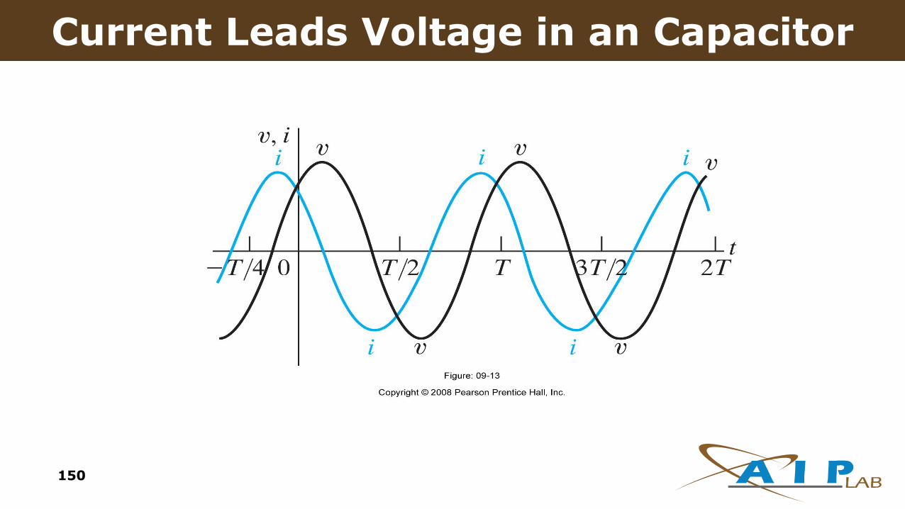
Current Leads Voltage in an Capacitor
150
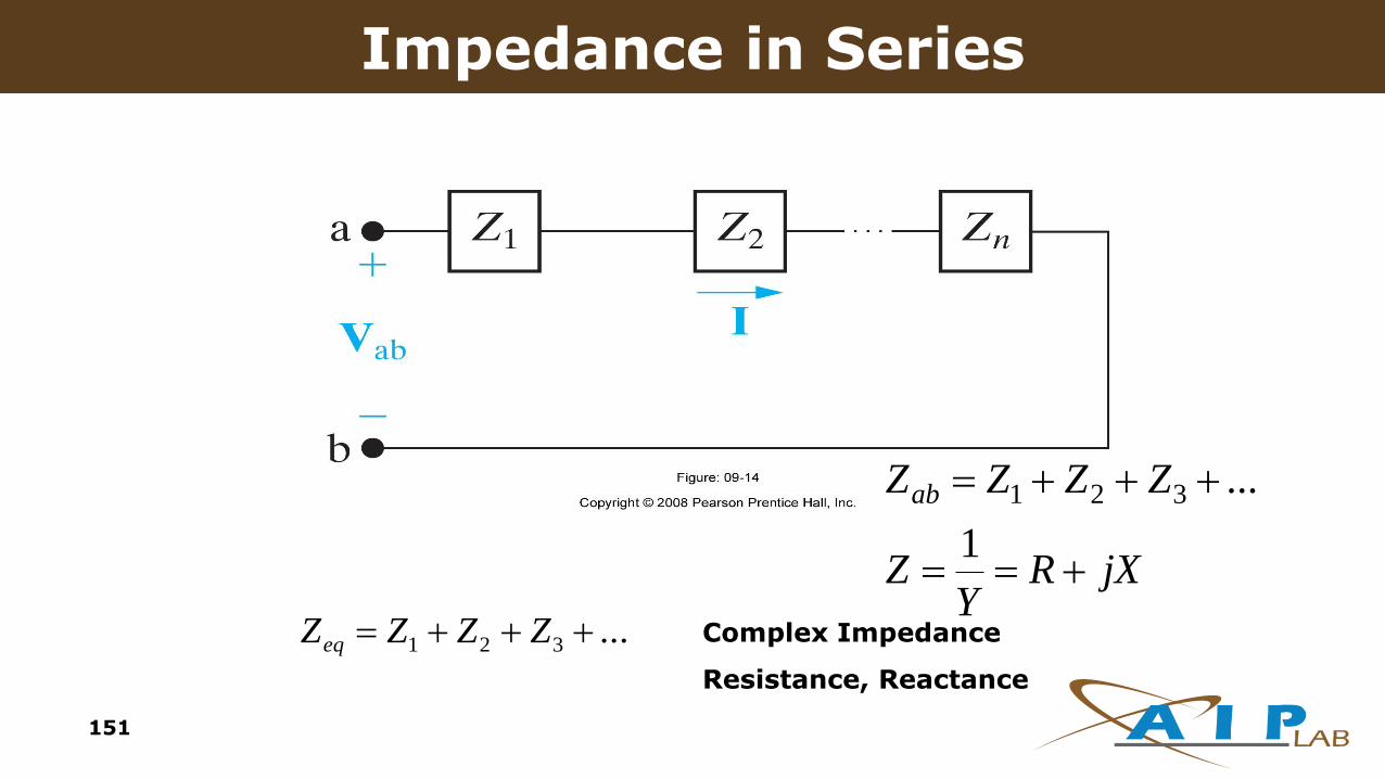
...321 ZZZZeqComplex Impedance
Resistance, Reactance
Impedance in Series
151
jXRY
Z
ZZZZab
1
...321

...1111
321
ZZZZab
jBGZ
Y
YYYYab
1
...321
Complex Admittance
Conductance, Susceptance
Impedance in Parallel
152

Thevenin and Norton Transformation
153
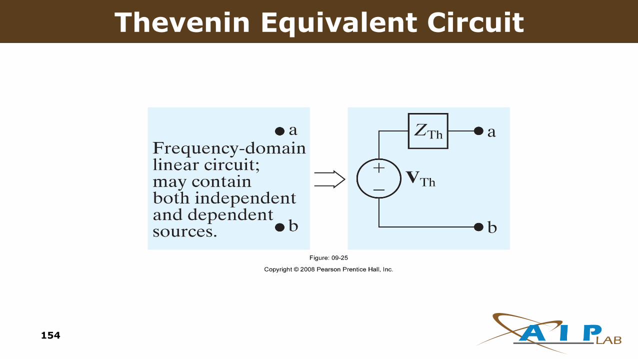
Thevenin Equivalent Circuit
154
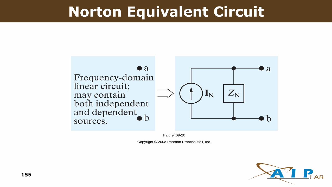
Norton Equivalent Circuit
155

2221
2111
)(0
)(
IZLjRMIj
MIjILjRZV
L
ss
L
r
rab
ZLjR
MZ
ZLjRZ
22
22
11
Time differentiation replaced by j
Transformer
156

1
2
1
2
N
N
v
v
1
2
2
1
N
N
i
i
Power Conserved
Sinusoidal Ideal Transformer

158
1ST ORDER FILTER ANALYSIS

Figure 14.2 A circuit with voltage
input and output.
Filtering Circuit
159
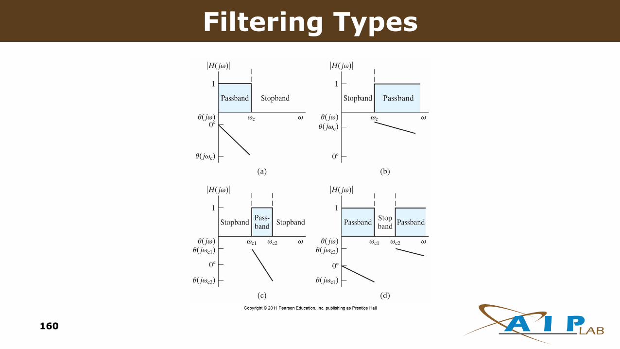
response plots of the four types of filter
circuits. (a) An ideal low-pass filter. (b)
An ideal high-pass filter. (c) An ideal
bandpass filter. (d) An ideal bandreject
filter.
Filtering Types
160

Figure 14.4 (a) A series RL low-pass
filter. (b) The equivalent circuit at = 0
and (c) The equivalent circuit at = .
Low-Pass Filtering Analysis
161

Figure 14.5 The frequency response
plot for the series RL circuit in Fig.
14.4(a).
Magnitude & Phase Responses
162

Figure 14.6 The s-domain equivalent
for the circuit in Fig. 14.4(a).
LR Transfer Function Analysis
163

Figure 14.7 A series RC low-pass
filter.
Low-Pass Passive RC Circuit
164
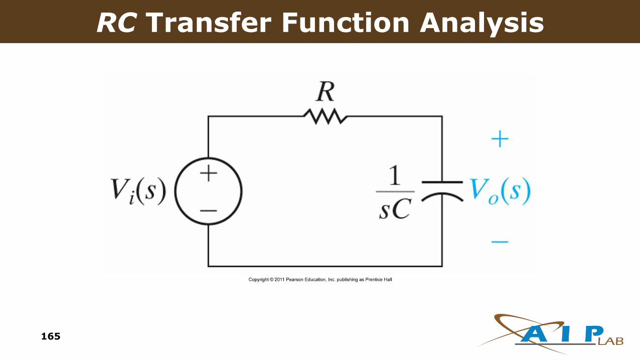
Figure 14.8 The s-domain equivalent
for the circuit in Fig. 14.7.
RC Transfer Function Analysis
165
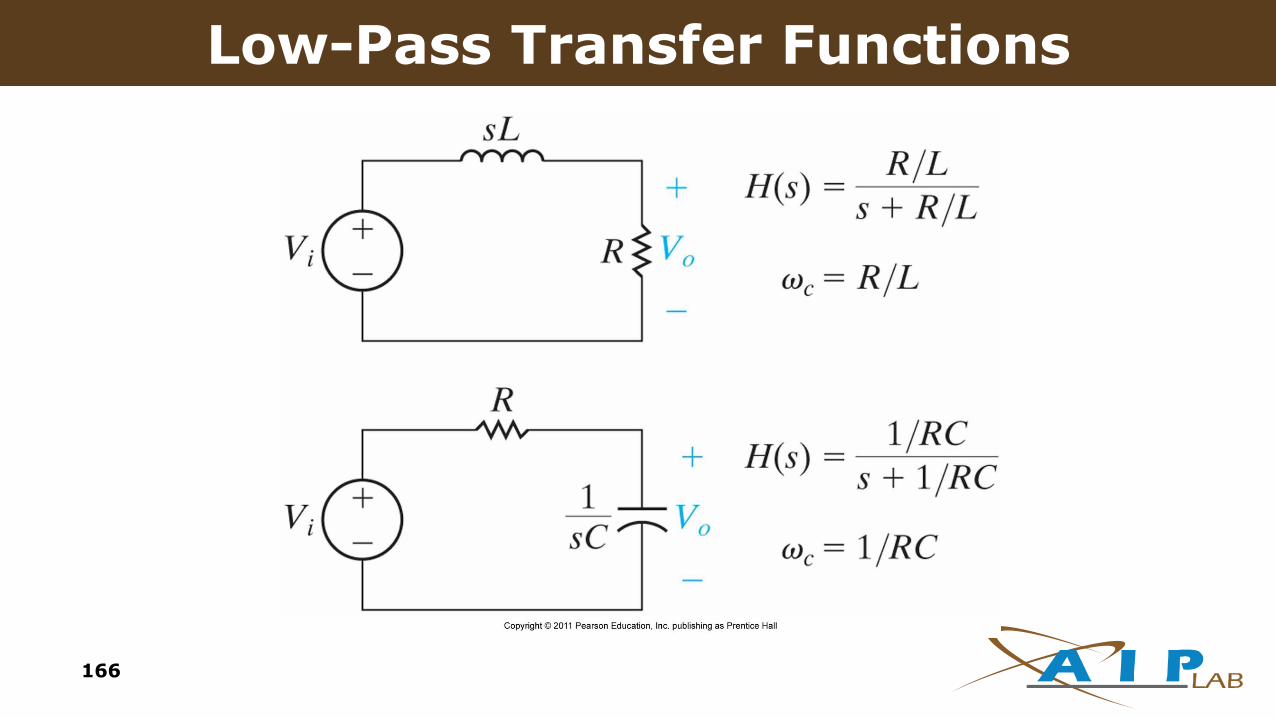
Figure 14.9 Two low-pass filters, the
series RL and the series RC, together
with their transfer functions and
cutoff frequencies.
Low-Pass Transfer Functions
166

Passive low-pass filter with cut-off frequency
First Order Low-Pass RC Passive Filter
167

Figure 14.10 A series RC high-pass
filter; (b) the equivalent circuit at = 0;
and (c) the equivalent circuit at = .
High-Pass Filtering Analysis
168
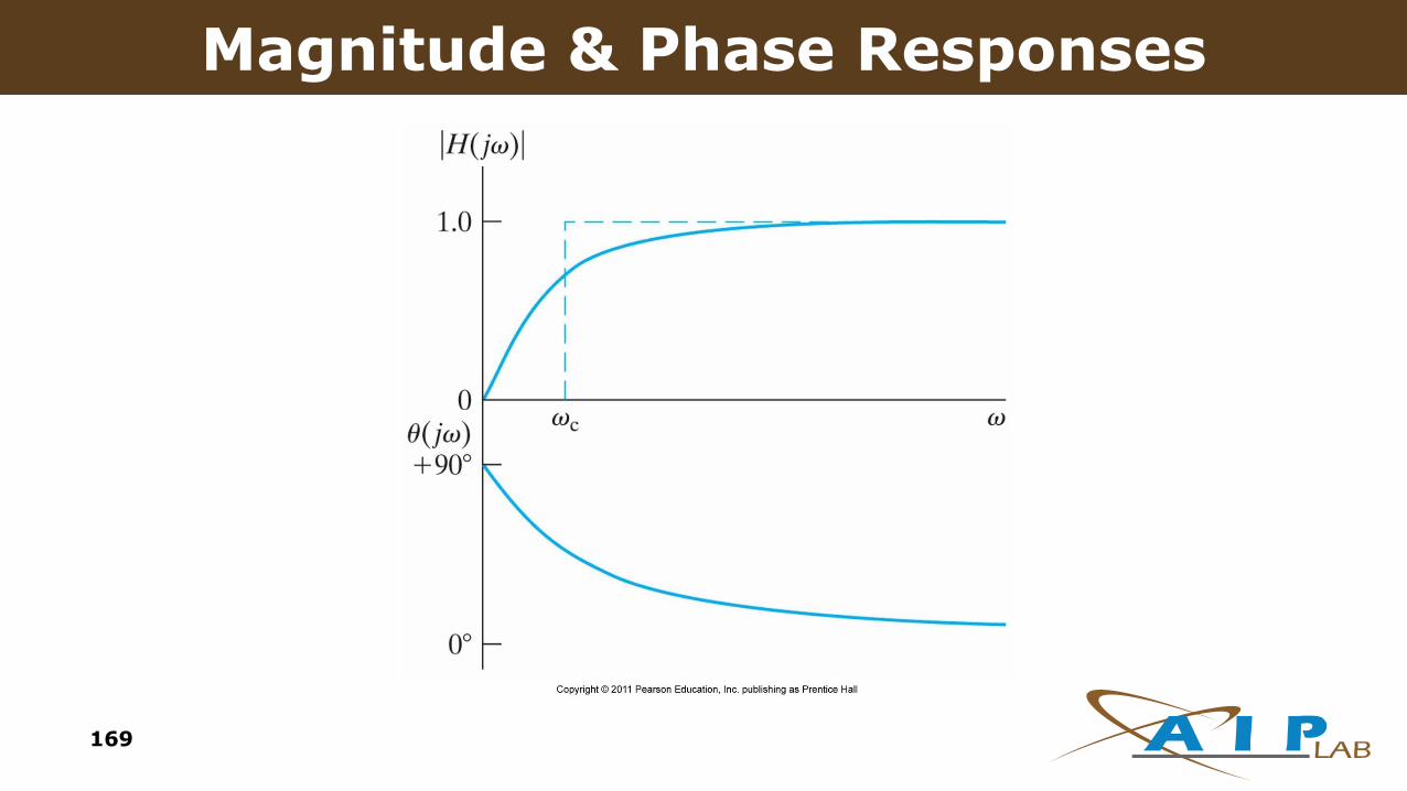
Figure 14.11 The frequency response
plot for the series RC circuit in Fig.
14.10(a).
Magnitude & Phase Responses
169
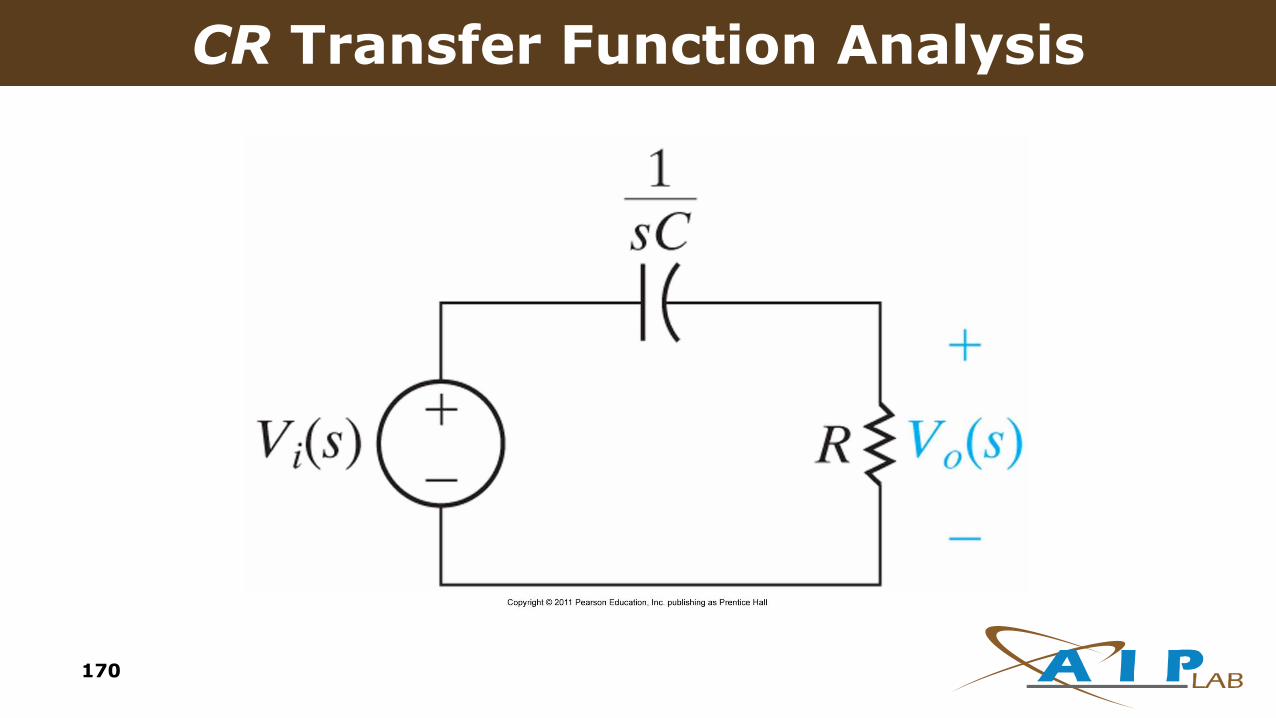
Figure 14.12 The s-domain
equivalent of the circuit in Fig. 14.10(a).
CR Transfer Function Analysis
170
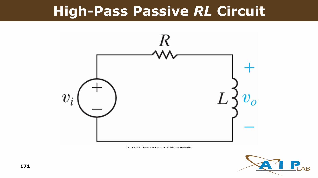
Figure 14.13 The circuit for Example
14.3.
High-Pass Passive RL Circuit
171

Figure 14.14 The s-domain
equivalent of the circuit in Fig. 14.13.
RL Transfer Function Analysis
172

173
First-Order Filter Circuits
L+
–VS
C
R
Low Pass
High
Pass
HR = R / (R + sL)
HL = sL / (R + sL)
+
–VS
R
High Pass
Low
Pass
GR = R / (R + 1/sC)
GC = (1/sC) / (R + 1/sC)

174
2nd ORDER FILTER ANALYSIS
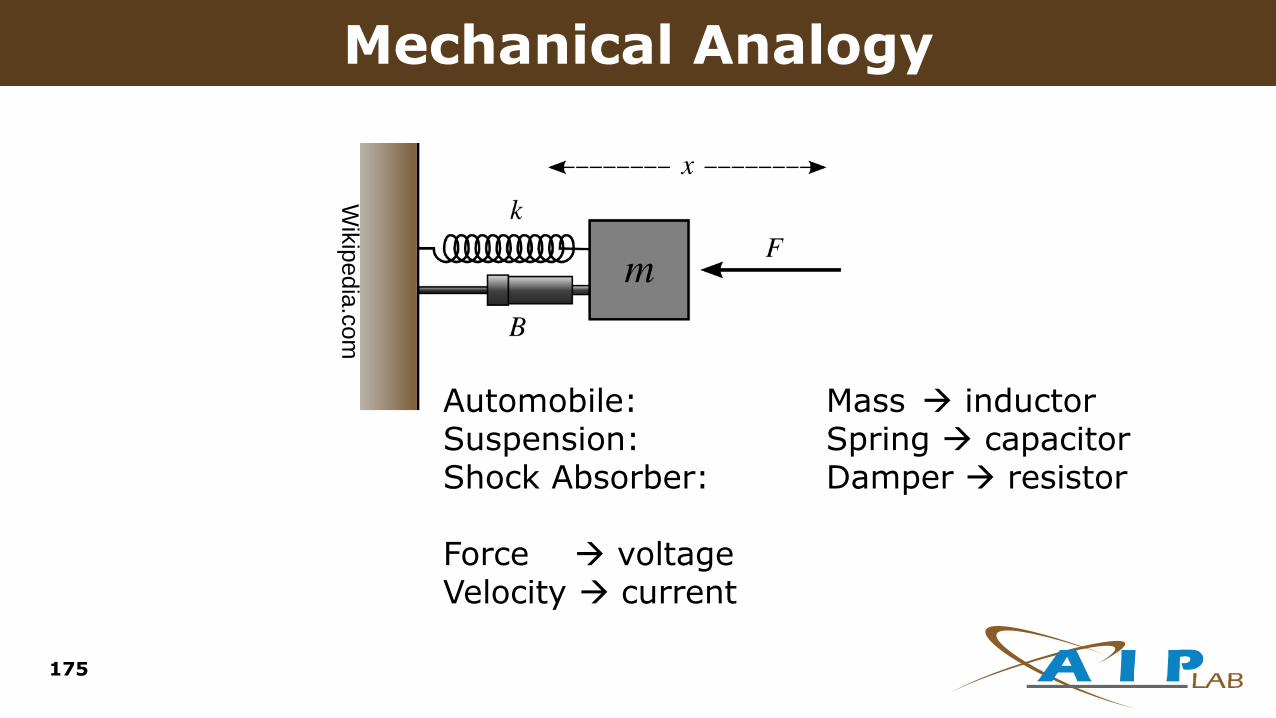
Mechanical Analogy
Automobile: Mass inductorSuspension: Spring capacitorShock Absorber: Damper resistor
Force voltageVelocity current
Wik
ipedia
.com
175

Series RLC Circuit
+
-VS(t)
L
C
Ri(t)
KVL:
VL + VR + VC = Vs
176

dt
dv
LLC
ti
dt
di
L
R
dt
id
dt
dv
C
ti
dt
diR
dt
idL
tvvdttiC
iRdt
diL
tvtvtvtv
S
S
t
SC
SCRL
1)(
0)(
)()0()(1
)()()()(
2
2
2
2
0
177
Series RLC Circuit Equations

0)(2
0:
.1
2...
1)(2
1)(
202
2
0
202
2
2
2
tidt
di
dt
id
vresponsenaturaltheFind
LCand
L
Rwhere
dt
dv
Lti
dt
di
dt
id
dt
dv
LLC
ti
dt
di
L
R
dt
id
S
S
S
178
Series RLC Circuit Equations

2
0
2
2
0
2
2
0
2
2
0
2
2
02
2
)1(2
)1(4)2(2
:
02
:
02
:
)(
:
0)(2
s
equationquadratictheUse
ss
giving
keskekes
ngsubstituti
keti
formtheinsolutionatry
tidt
di
dt
id
ststst
st
179
Series RLC Circuit Equations

Natural Overdamped Case
180
Case 1 - Overdamped: >o large R:LCL
R 1
2>
tsts
n eKeKti
s
s
21
21
2
0
2
2
2
0
2
1
)(
:lsexponentia decaying twois response natural The
0
0
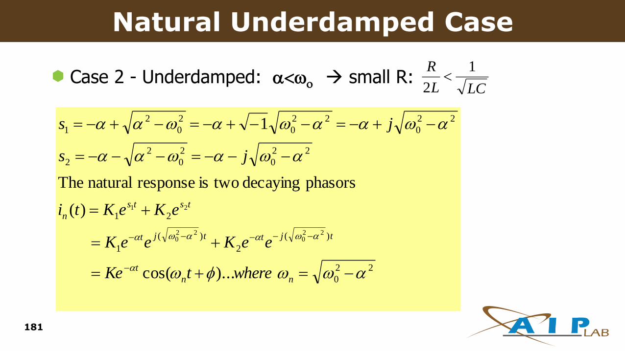
Natural Underdamped Case
181
LCL
R 1
2
22
0
)(
2
)(
1
21
22
0
2
0
2
2
22
0
22
0
2
0
2
1
)...cos(
)(
phasorsdecayingtwoisresponsenaturalThe
1
220
220
21
nn
t
tjttjt
tsts
n
wheretKe
eeKeeK
eKeKti
js
js
Case 2 - Underdamped: o small R:
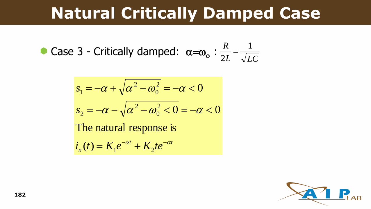
Natural Critically Damped Case
182
LCL
R 1
2
tt
n teKeKti
s
s
21
2
0
2
2
2
0
2
1
)(
isresponsenaturalThe
00
0
Case 3 - Critically damped: o :
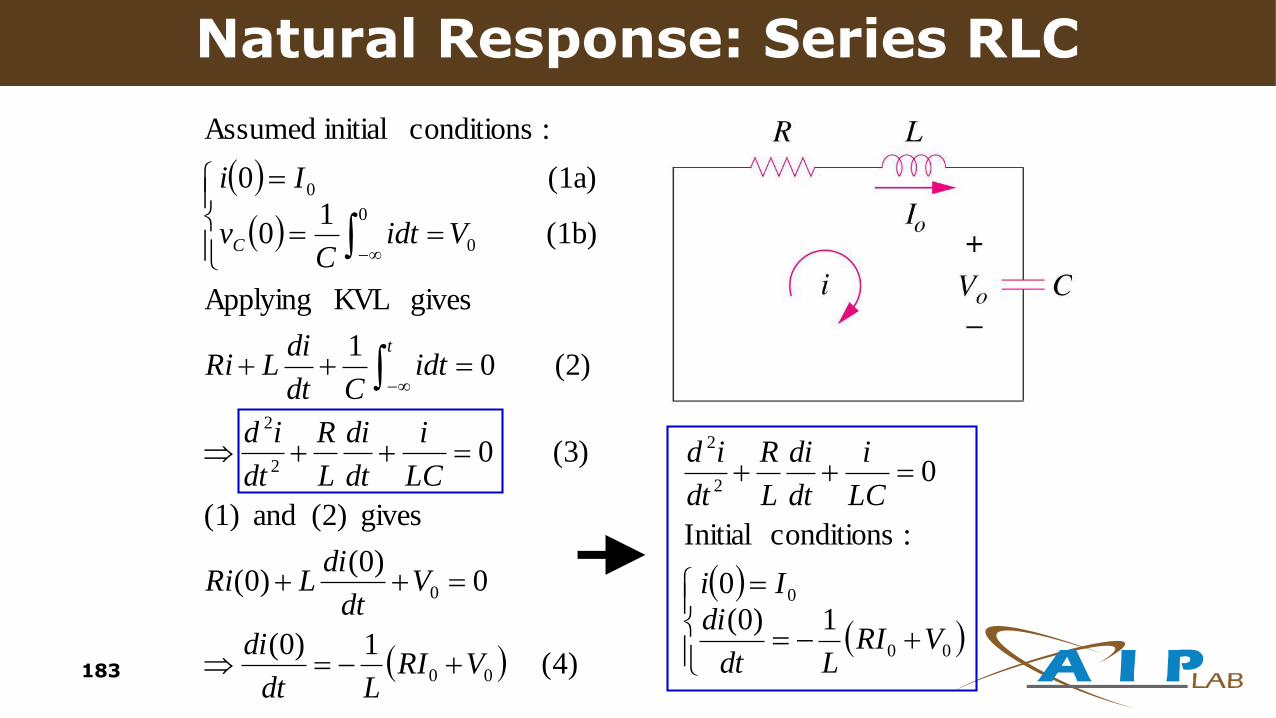
)4( 1)0(
0)0(
)0(
gives (2) and (1)
(3) 0
(2) 01
gives KVL Applying
(1b)
10
(1a) 0
: conditions initial Assumed
00
0
2
2
0
0
0
VRILdt
di
Vdt
diLRi
LC
i
dt
di
L
R
dt
id
idtCdt
diLRi
VidtC
v
Ii
t
C
00
0
2
2
1)0(
0
: conditions Initial
0
VRILdt
di
Ii
LC
i
dt
di
L
R
dt
id
Overdamped CaseNatural Response: Series RLC
183
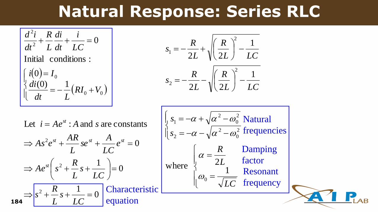
01
01
0
constants are and : Let
1)0(
0
: conditions Initial
0
2
2
2
00
0
2
2
LCs
L
Rs
LCs
L
RsAe
eLC
Ase
L
AReAs
sAAei
VRILdt
di
Ii
LC
i
dt
di
L
R
dt
id
st
ststst
st
LC
L
R
s
s
LCL
R
L
Rs
LCL
R
L
Rs
1
2 where
1
22
1
22
0
2
0
2
2
2
0
2
1
2
2
2
1
Characteristic
equation
Natural
frequencies
Damping
factor
Resonant
frequency
Natural Response: Series RLC
184
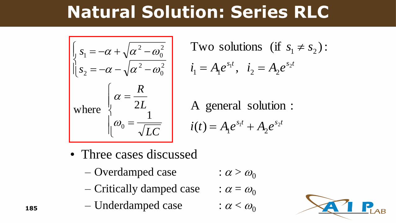
tsts
tsts
eAeAti
eAieAi
ss
21
21
21
2211
21
)(
:solution generalA
,
:) (if solutions Two
LC
L
R
s
s
1
2 where
0
2
0
2
2
2
0
2
1
• Three cases discussed
– Overdamped case : > 0
– Critically damped case : = 0
– Underdamped case : < 0
Natural Solution: Series RLC
185
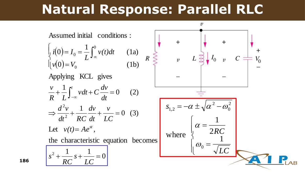
011
becomesequation sticcharacteri the
,Let
(3) 01
(2) 01
gives KCL Applying
(1b) 0
(1a) 1
0
: conditions initial Assumed
2
2
2
0
0
0
LCs
RCs
Aev(t)
LC
v
dt
dv
RCdt
vd
dt
dvCvdt
LR
v
Vv
v(t)dtL
Ii
st
t
LC
RC
s
1
2
1
where
0
2
0
2
2,1
Natural Response: Parallel RLC
186

• Overdamped case : > 0
• Critically damped case : = 0
• Underdamped case : < 0
tstseAeAtv 21
21)(
tetAAtv 21)(
tAtAetv
js
dd
t
d
d
sincos)(
where
21
22
0
2,1
Natural Response: Parallel RLC
187
L
RIV
dt
di
Ii
LC
L
R
s
00
0
0
2
0
2
2,1
)0(
)0(
:conditions Initial
1
2 where
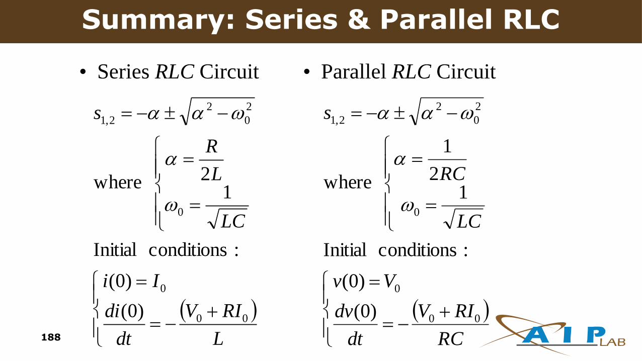
• Series RLC Circuit • Parallel RLC Circuit
RC
RIV
dt
dv
Vv
LC
RC
s
00
0
0
2
0
2
2,1
)0(
)0(
:conditions Initial
1
2
1
where
Summary: Series & Parallel RLC
188

case. free-source in the
as form same thehas (2)
(2)
But
(1)
,0for KVL Applying
2
2
LC
V
LC
v
dt
dv
L
R
dt
vd
dt
dvCi
Vvdt
diLRi
t
S
S
>
response state-steady the:
response transientthe:
where
)()()(
ss
t
sst
v
v
tvtvtv
Step Response: Series RLC
189

case. free-source in the as Same
01
becomesequation sticcharacteri The
0
, Let
0
2
''
2
'2
'
2
2
LCs
L
Rs
LC
v
dt
dv
L
R
dt
vd
Vvv
LC
Vv
dt
dv
L
R
dt
vd
S
S
Step Response: Series RLC
190

.)0( and )0( from obtained are where
sincos
)(
)()(
)()()(
2,1
21
21
2121
/dtdvvA
etAtA
etAA
eAeA
tv
Vvtv
tvtvtv
t
dd
t
tsts
t
Sss
sst
(Overdamped)
(Critically damped)
(Underdamped)
Step Response: Series RLC
191
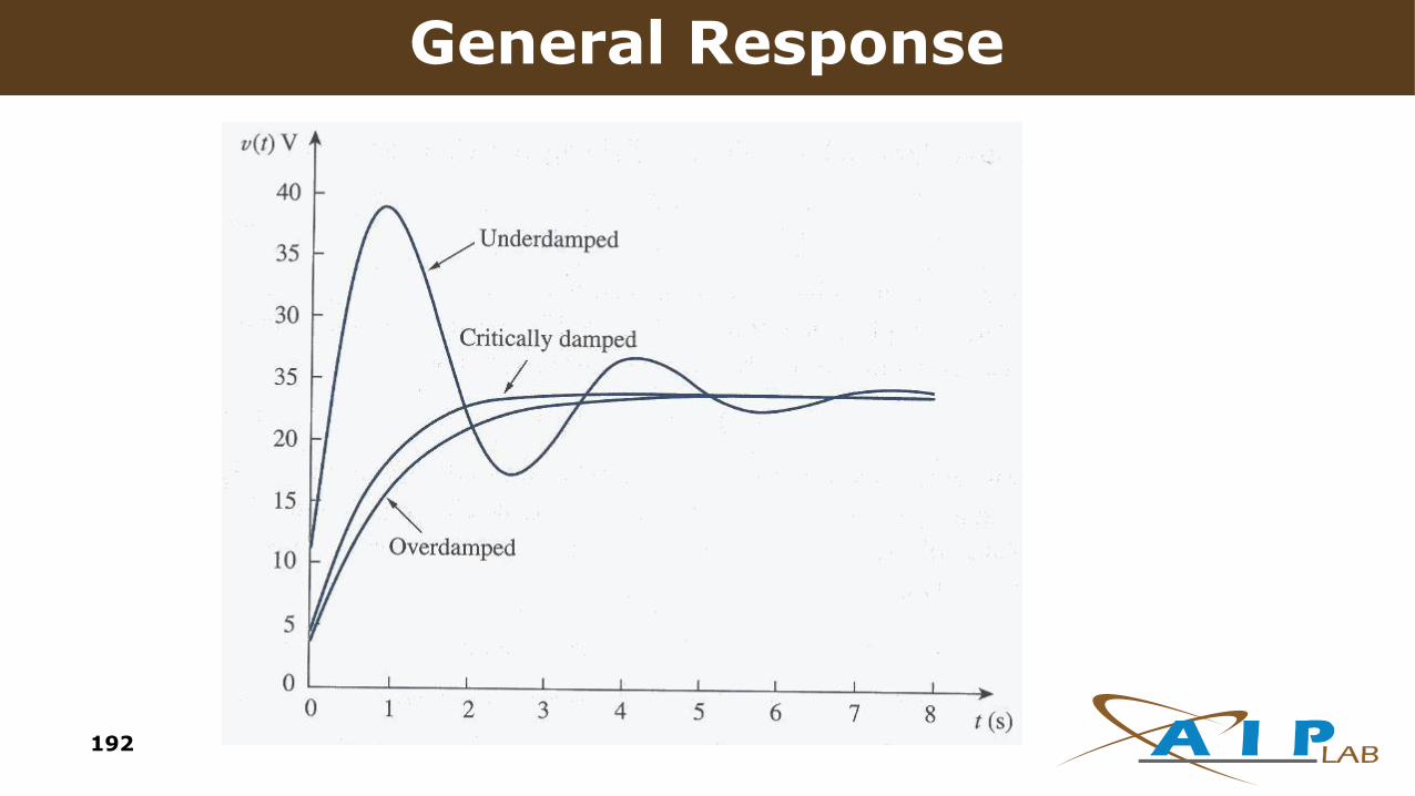
General Response
192

case. free-source in the
as form same thehas (2)
(2) 1
But
(1)
,0for KCL Applying
2
2
LC
I
LC
i
dt
di
RCdt
id
dt
diLv
Idt
dvCi
R
v
t
S
S
>
response state-steady the:
response transient the:
where
)()()(
ss
t
sst
i
i
tititi
Step Response: Parallel RLC
193
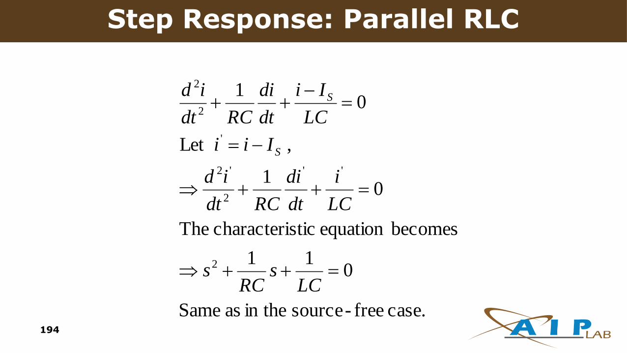
case. free-source in the as Same
011
becomesequation sticcharacteri The
01
, Let
01
2
''
2
'2
'
2
2
LCs
RCs
LC
i
dt
di
RCdt
id
Iii
LC
Ii
dt
di
RCdt
id
S
S
Step Response: Parallel RLC
194
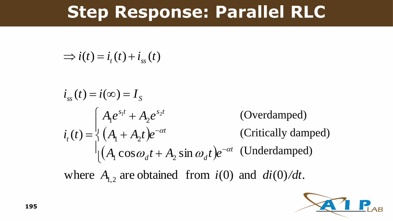
.)0( and )0( from obtained are where
sincos
)(
)()(
)()()(
2,1
21
21
2121
/dtdiiA
etAtA
etAA
eAeA
ti
Iiti
tititi
t
dd
t
tsts
t
Sss
sst
(Overdamped)
(Critically damped)
(Underdamped)
Step Response: Parallel RLC
195

196
Second-Order Filter Circuits
C
+
–VS
R
Band Pass
Low
Pass
LHigh
Pass
Band
Reject
Z = R + 1/sC + sL
HBP = R / Z
HLP = (1/sC) / Z
HHP = sL / Z
HBR = HLP + HHP
f
f
f
fjQ
ffjQ
LCfff
f
R
Lfj
fRC
j
fH
LCfff
f
R
Lfj
fRC
j
fC
jfLjR
fC
j
ZZZ
Z
S
S
in
out
inininCLR
Cout
0
0
0
00
0
00
0
1
)/(
2
121
2)(
2
121
2
22
2
V
V
VVVV
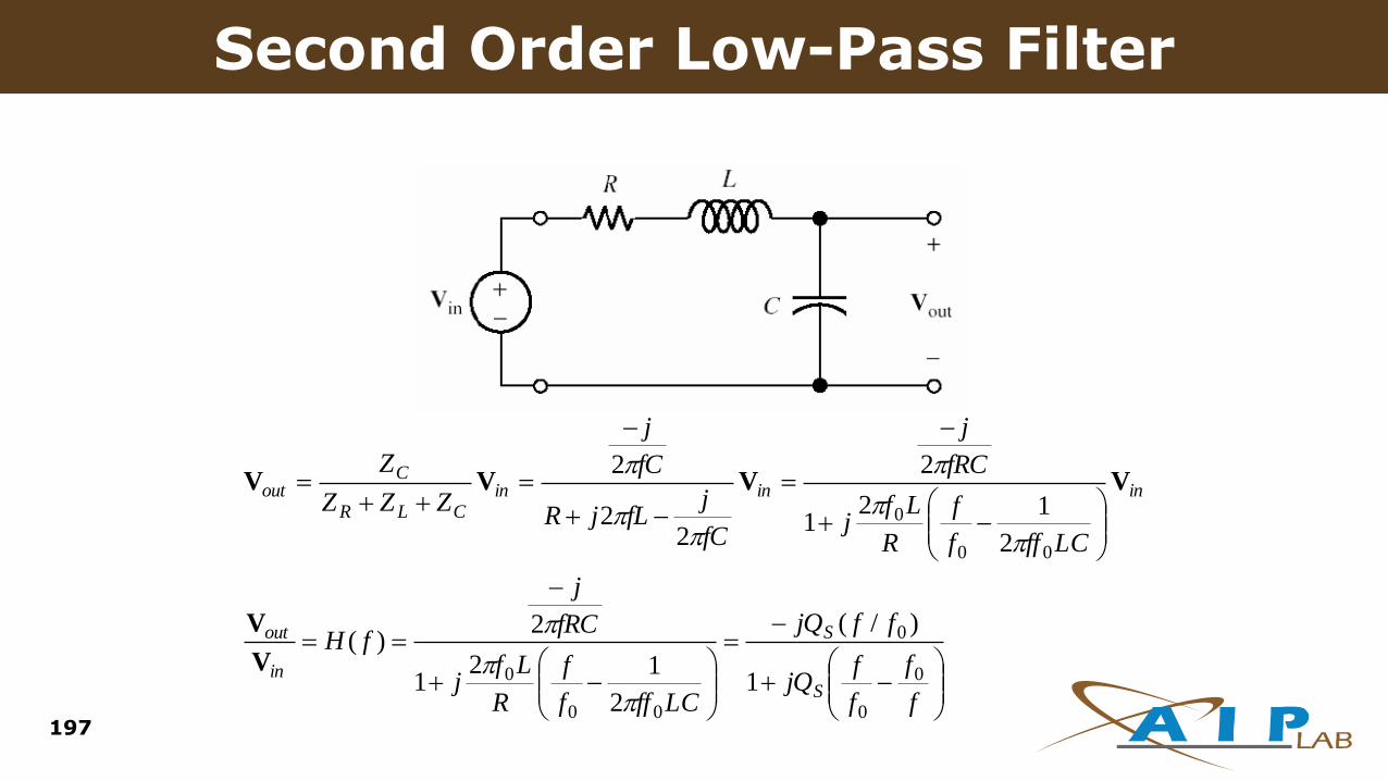
First-Order Filter CircuitsSecond Order Low-Pass Filter
197

Second-Order Low-Pass Filter
200
2
0
0012
002
0
00
0
1
1
90
1
ffffQ
ffQfH
ffffQTanffffQ
ffQ
ffffjQ
ffjQfH
S
s
sS
s
s
s
in
out
V
V
Low-Pass Filter: Natural Frequency
198

First-Order Filter CircuitsLow-Pass Filter: Natural Frequency
199

Second Order High-Pass Filter
At low frequency the
capacitor is an open circuit
At high frequency the
capacitor is a short and the
inductor is open
High-Pass Filter: Natural Frequency
200

Second Order Band-Pass Filter
At low frequency the
capacitor is an open circuit
At high frequency the
inductor is an open circuit
Band-Pass Filter: Natural Frequency
201

Second Order Band-Reject Filter
At low frequency the
capacitor is an open
circuit
At high frequency the
inductor is an open
circuit
Band-Reject Filter: Natural Frequency
202

203
Series RLC Bandpass Filter DesignDesign a series RLC bandpass filter with cutoff frequencies f1=1kHz and f2 = 10 kHz.
Cutoff frequencies give us two equations but we have 3 parameters to choose.
Thus, we need to select a value for either R, L, or C and use the equations to find
other values. Here, we choose C=1μF.
0 1 2
0
22 6
0
2 1
3
2 6 2
(6280)(62800) 19,867rad/s
3162.28Hz2
1 12.533 mH
2 (3162.28) (10 )
19,867rad/s0.3514
(2 *10000 2 *1000)rad/s
2.533(10 )143.24
(10 )(0.3514)
o
o
f
LC
Q
LR
CQ
f1=1kHz 1 = 2f1 = 6280 rad/s
f2 = 10 kHz 2 = 2f2 = 62,800 rad/s
0 1 2
0
2 1
Q
0
1
LC
0
2
1L L L LR
Q Q C Q CQ LC

204
ACTIVE FILTER DESIGN

ffB
Bi
f
ffi
f
i
f
ff
f
f
f
ff
f
f
ff
i
f
i
o
CRf
ffjR
R
CfRjR
R
Z
ZfH
CfRj
RZ
R
CfRj
R
fCj
RZ
Z
Z
V
VfH
2
1
)/(1
1
21
1)(
21
21
2
1
111
)(
A low-pass filter with a dc gain of -Rf/Ri
First Order Low-Pass Active RC Filter
205

dttvRC
tv
t
o in
0
1
Integrator Circuit
206
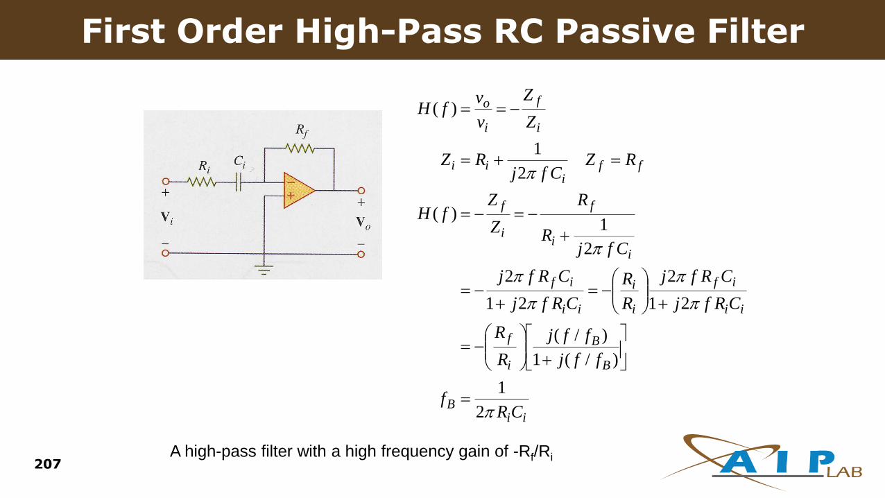
iiB
B
B
i
f
ii
if
i
i
ii
if
ii
f
i
f
ffi
ii
i
f
i
o
CRf
ffj
ffj
R
R
CRfj
CRfj
R
R
CRfj
CRfj
CfjR
R
Z
ZfH
RZCfj
RZ
Z
Z
v
vfH
2
1
)/(1
)/(
21
2
21
2
2
1)(
2
1
)(
A high-pass filter with a high frequency gain of -Rf/Ri
First Order High-Pass RC Passive Filter
207

dt
dvRCtvo
in
Differentiator Circuit
208
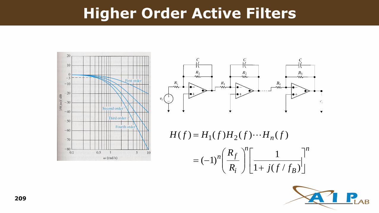
n
B
n
i
fn
n
ffjR
R
fHfHfHfH
)/(1
1)1(
)()()()( 21
Higher Order Active Filters
209
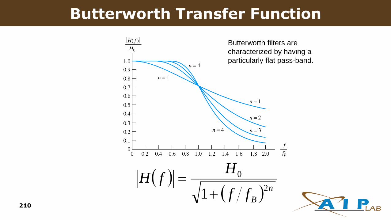
n
Bff
HfH
2
0
1
Butterworth filters are
characterized by having a
particularly flat pass-band.
Butterworth Transfer Function
210
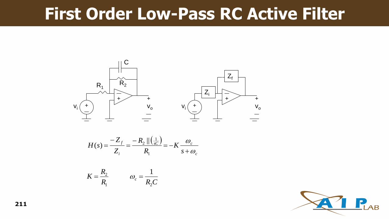
211
First Order Low-Pass RC Active Filter
+
+
+
vovi
R1R2
C
+
+
+
vovi
Zi
Zf
c
csC
i
f
sK
R
R
Z
ZsH
1
12 ||
)(
CRR
RK c
21
2 1
212
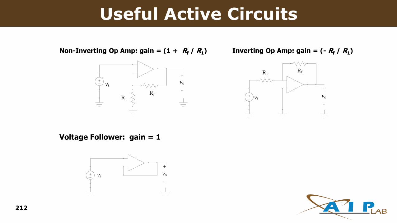
Useful Active Circuits
Non-Inverting Op Amp: gain = (1 + Rf / R1) Inverting Op Amp: gain = (- Rf / R1)
Voltage Follower: gain = 1
vi
+
vo
-Rf
R1 vi
+
vo
-
RfR1
vi
+
vo
-

213
Other Useful Active Circuits
The summing amp: The differential amp:
-
+
vi1
vi2
viN
+
vo
-
R1
R2
RN
Rf
vi1
vi2
+
vo
-
R1
R2
R1
R2
vR
Rv
R
Rv
R
Rvo
f
i
f
i
f
N
iN
1
1
2
2 vR
Rv vo i i 2
1
2 1

214
First Order Filter Functions
215
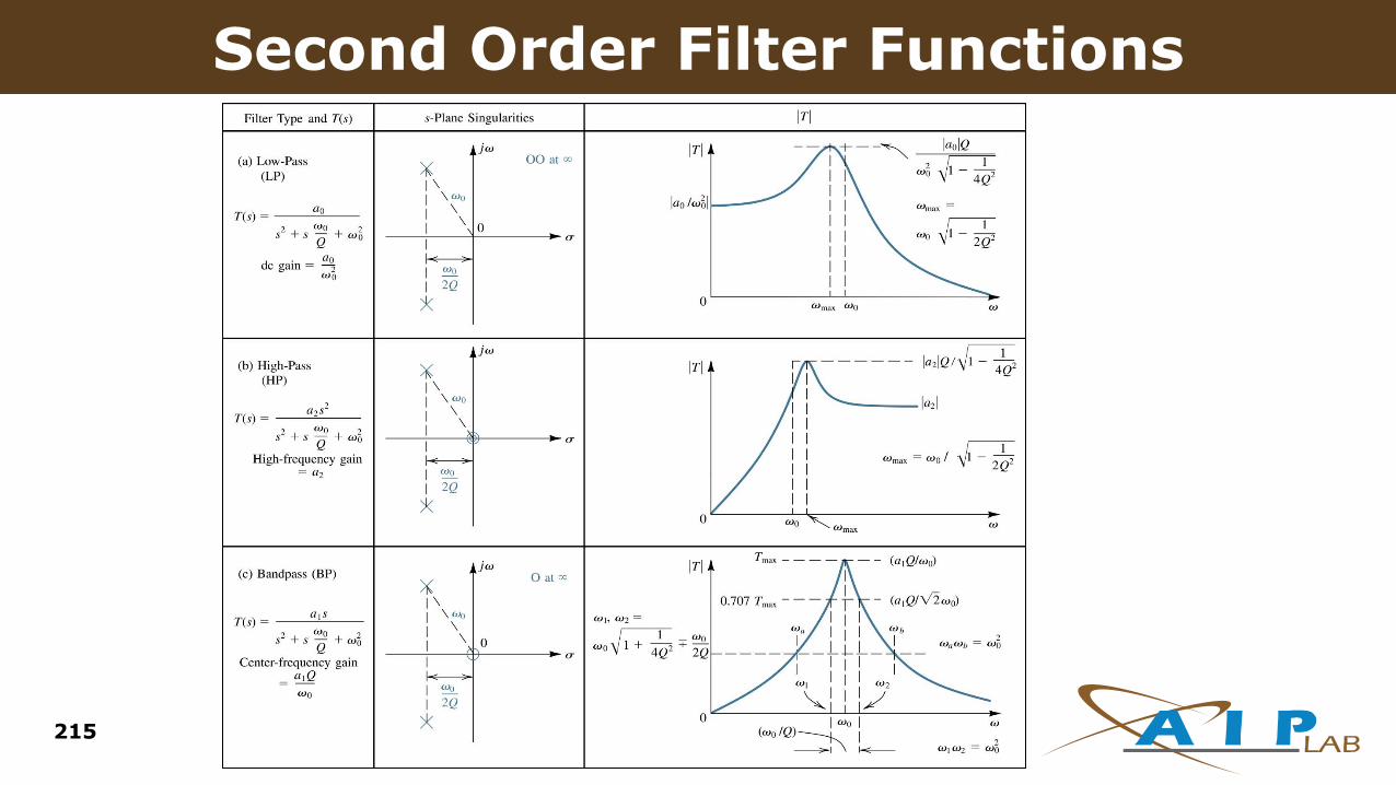
Second Order Filter Functions
216
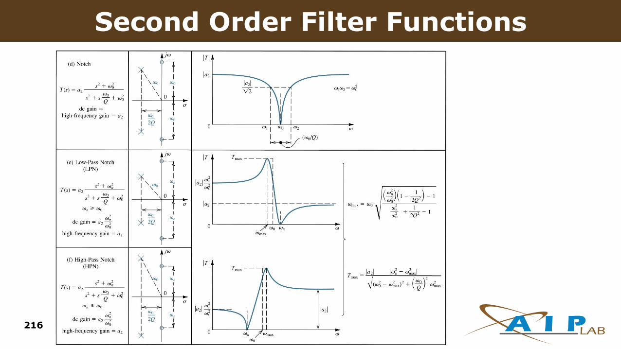
Second Order Filter Functions

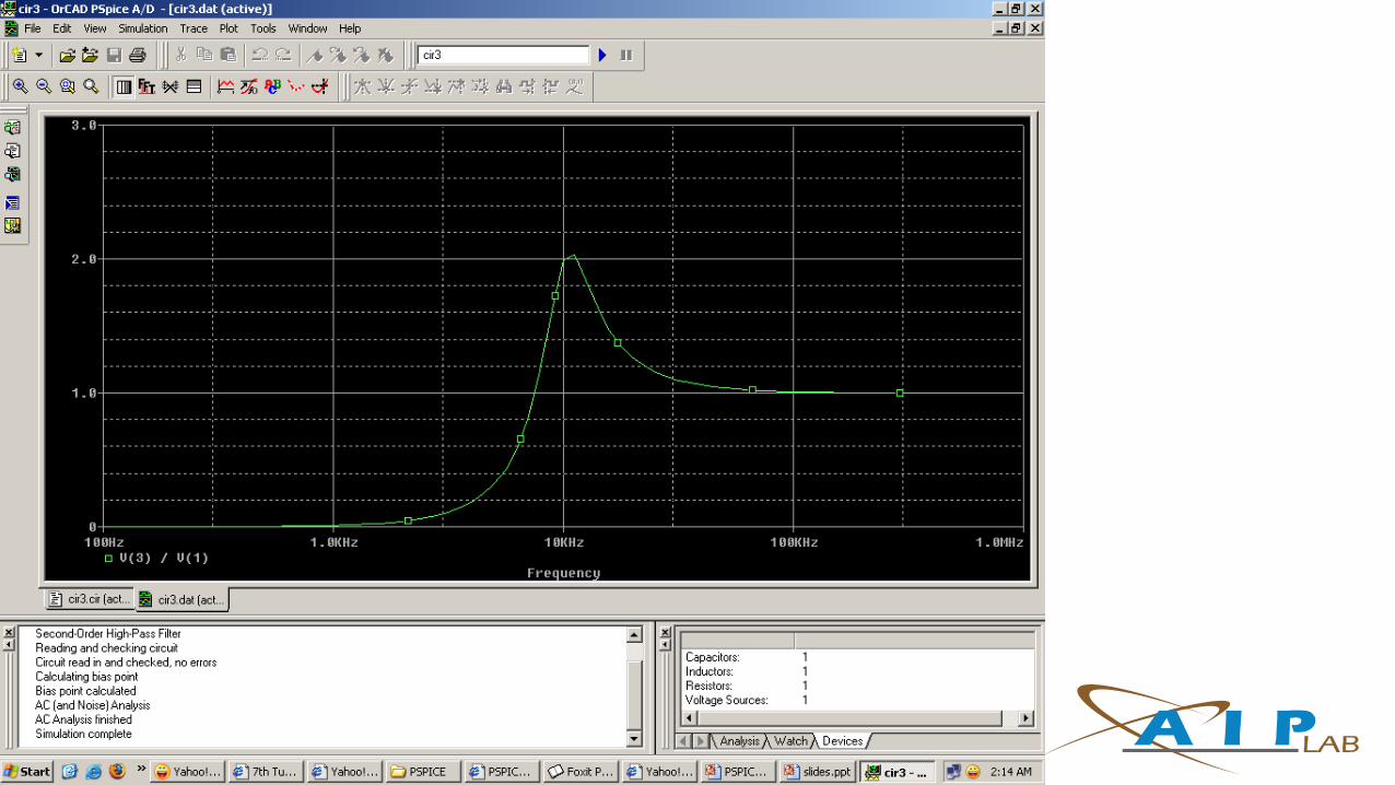
AC Analysis
Second-Order High-Pass Filter
Vin 1 0 AC 10V
Rf 1 2 4.0
Cf 2 3 2.0uF
Lf 3 0 127uH
.AC DEC 20 100Hz 1MEG
.PROBE
.END
217


THANK YOU
220
PART of this document’s CONTENT is NOT ORIGINAL.Its ORIGINATION is from many FRIENDLY SOURCES.THANKS to ALL the sources used for the compositionof this document. WE are TRULY INDEBTED to YOU.
http://www.ece.uprm.edu/~domingo/