figure 6.1 a scan (or point cloud) created by a laser scanner
TRANSCRIPT

Figure 6.1 A scan (or point cloud) created by a laser scanner.

Figure 6.2 The wall surface in (a) is analyzed according to (b) data density, (c) occlusion regions, (d) data uncertainty, and (e) deviation from the ideal
planar wall.
(a) (b) (c)
(d) (e)

Figure 6.3 Laser scanners difficulties: (a) mixed pixels create phantom points at object boundaries; (b) reflections in a mirror create a wall surface
extending beyond the room boundary.
(a) (b)
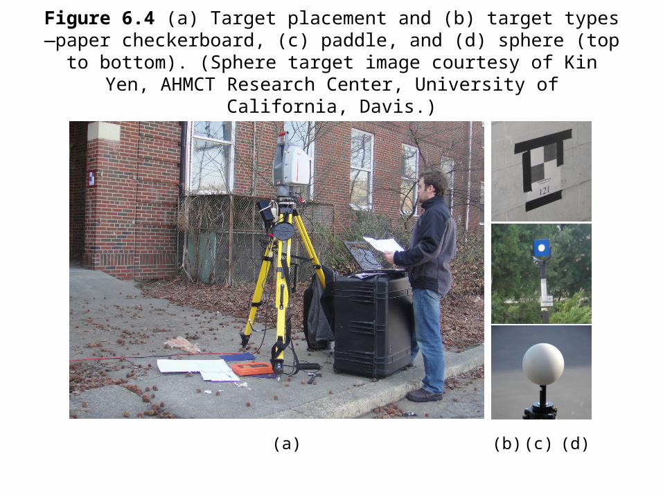
Figure 6.4 (a) Target placement and (b) target types—paper checkerboard, (c) paddle, and (d) sphere (top to bottom). (Sphere target image courtesy of
Kin Yen, AHMCT Research Center, University of California, Davis.)
(a) (b) (c) (d)

Figure 6.5 Five registered scans. (Image courtesy of Intelisum, Inc.)

Figure 6.6 Two common modeling techniques are sectioning and surface fitting: (a) sectioning; (b) surface fitting; (c) resulting BIM, in Autodesk Revit
(adapted from Tang, P., et al., “Automatic Reconstruction of As-built Building Information Models from Laser-Scanned Point Clouds: A Review of Related
Techniques,” Automation in Construction, Vol. 19, No. 7, November 2010, pp. 829–843).
(a) (b) (c)

Figure 6.7 Quality assurance (QA) through visualization: large deviations in the window regions (1), at a setback (2), and a door (3) (adapted from Anil,
E., et al., “Assessment of Quality of As-is Building Information Models Generated
from Point Clouds Using Deviation Analysis,” in Proceedings of the SPIE Vol. 7864A, Electronics Imaging Science and Technology Conference (IS&T), 3D
Imaging Metrology, San Francisco, CA, January 2011).

Figure 6.8 Walls, floors, ceilings, and clutter objects were automatically segmented and recognized from point cloud data.
(a) (b)