Fighting Boredom in Recommender Systems withLinear Reinforcement Learning

Romain Warlopfifty-five, Paris, France

SequeL Team, Inria Lille, Franceromain@fifty-five.com

Alessandro LazaricFacebook AI Research

Paris, Francelazaric@fb.com

Jérémie MaryCriteo AI LabParis, France

j.mary@criteo.com

Abstract

A common assumption in recommender systems (RS) is the existence of a bestfixed recommendation strategy. Such strategy may be simple and work at the itemlevel (e.g., in multi-armed bandit it is assumed one best fixed arm/item exists) orimplement more sophisticated RS (e.g., the objective of A/B testing is to find thebest fixed RS and execute it thereafter). We argue that this assumption is rarelyverified in practice, as the recommendation process itself may impact the user’spreferences. For instance, a user may get bored by a strategy, while she may gaininterest again, if enough time passed since the last time that strategy was used. Inthis case, a better approach consists in alternating different solutions at the rightfrequency to fully exploit their potential. In this paper, we first cast the problem asa Markov decision process, where the rewards are a linear function of the recenthistory of actions, and we show that a policy considering the long-term influenceof the recommendations may outperform both fixed-action and contextual greedypolicies. We then introduce an extension of the UCRL algorithm (LINUCRL) toeffectively balance exploration and exploitation in an unknown environment, andwe derive a regret bound that is independent of the number of states. Finally,we empirically validate the model assumptions and the algorithm in a number ofrealistic scenarios.

1 Introduction

Consider a movie recommendation problem, where the recommender system (RS) selects the genreto suggest to a user. A basic strategy is to estimate user’s preferences and then recommend movies ofthe preferred genres. While this strategy is sensible in the short term, it overlooks the dynamics of theuser’s preferences caused by the recommendation process. For instance, the user may get bored ofthe proposed genres and then reduce her ratings. This effect is due to the recommendation strategyitself and not by an actual evolution of user’s preferences, as she would still like the same genres, ifonly they were not proposed so often.1

The existence of an optimal fixed strategy is often assumed in RS using, e.g., matrix factorization toestimate users’ ratings and the best (fixed) item/genre [16]. Similarly, multi-armed bandit (MAB)algorithms [4] effectively trade off exploration and exploitation in unknown environments, but stillassume that rewards are independent from the sequence of arms selected over time and they tryto select the (fixed) optimal arm as often as possible. Even when comparing more sophisticatedrecommendation strategies, as in A/B testing, we implicitly assume that once the better option(either A or B) is found, it should be constantly executed, thus ignoring how its performance maydeteriorate if used too often. An alternative approach is to estimate the state of the user (e.g., her

1In this paper, we do not study non-stationarity preferences, as it is a somehow orthogonal problem to theissue that we consider.

32nd Conference on Neural Information Processing Systems (NeurIPS 2018), Montréal, Canada.

level of boredom) as a function of the movies recently watched and estimate how her preferences areaffected by that. We could then learn a contextual strategy that recommends the best genre dependingon the actual state of the user (e.g., using LINUCB [17]). While this could partially address theprevious issue, we argue that in practice it may not be satisfactory. As the preferences depend onthe sequence of recommendations, a successful strategy should “drive” the user’s state in the mostfavorable condition to gain as much reward as possible in the long term, instead selecting the best“instantaneous” action at each step. Consider a user with preferences 1) action, 2) drama, 3) comedy.After showing a few action and drama movies, the user may get bored. A greedy contextual strategywould then move to recommending comedy, but as soon as it estimates that action or drama arebetter again (i.e., their potential value reverts to its initial value as they are not watched), it wouldimmediately switch back to them. On the other hand, a more farsighted strategy may prefer to stickto comedy for a little longer to increase the preference of the user for action to its higher level andfully exploit its potential.

In this paper, we propose to use a reinforcement learning (RL) [23] model to capture this dynamicalstructure, where the reward (e.g., the average rating of a genre) depends on a state that summarizes theeffect of the recent recommendations on user’s preferences. We introduce a novel learning algorithmthat effectively trades off exploration and exploitation and we derive theoretical guarantees for it.Finally, we validate our model and algorithm in synthetic and real-data based environments.

Related Work. While in the MAB model, regret minimization [2] and best-arm identificationalgorithms [11, 22] have been often proposed to learn effective RS, they all rely on the assumptionthat one best fixed arm exists. [8] study settings with time-varying rewards, where each time an armis pulled, its reward decreases due to loss of interest, but, unlike our scenario, it never increases again,even if not selected for a long time. [14] also consider rewards that continuously decrease over timewhether the arm is selected or not (e.g., modeling novelty effects, where new products naturally looseinterest over time). This model fits into the more general case of restless bandit [e.g., 6, 25, 20],where each arm has a partially observable internal state that evolves as a Markov chain independentlyfrom the arms selected over time. Time-varying preferences has also been widely studied in RS.[25, 15] consider a time-dependent bias to capture seasonality and trends effect, but do not considerthe effects on users’ state. More related to our model is the setting proposed by [21], who consider anMDP-based RS at the item level, where the next item reward depends on the previously k selecteditems. Working at the item level without any underlying model assumption prevents their algorithmfrom learning in large state spaces, as every single combination of k items should be considered(in their approach this is partially mitigated by state aggregation). Finally, they do not considerthe exploration-exploitation trade-off and they directly solve an estimated MDP. This may lead toan overall linear regret, i.e., failing to learn the optimal policy. Somewhat similar, [12] propose asemi-markov model to decide what item to recommend to a user based on her latent psychologicalstate toward this item. They assumed two possible states: sensitization, state during which she ishighly engaged with the item, and boredom, state during which she is not interested in the item.Thanks to the use of a semi-markov model, the next state of the user depends on how long she hasbeen in the current state. Our work is also related to the linear bandit model [17, 1], where rewardsare a linear function of a context and an unknown target vector. Despite producing context-dependentpolicies, this model does not consider the influence that the actions may have on the state and thusoverlook the potential of long-term reward maximization.

2 Problem Formulation

We consider a finite set of actions a ∈ {1, . . . ,K} = [K]. Depending on the application, actionsmay correspond to simple items or complex RS. We define the state st at time t as the history of thelast w actions, i.e., st = (at−1, · · · , at−w), where for w = 0 the state reduces to the empty history.As described in the introduction, we expect the reward of an action a to depend on how often a hasbeen recently selected (e.g., a user may get bored the more a RS is used). We introduce the recencyfunction ρ(st, a) =

∑wτ=1 1{at−τ = a}/τ , where the effect of an action fades as 1/τ , so that the

recency is large if an action is often selected and it decreases as it is not selected for a while. Wedefine the (expected) reward function associated to an action a in state s as

r(st, a) =

d∑j=0

θ∗a,jρ(st, a)j = xTs,aθ∗a, (1)

2

0.0 0.5 1.0 1.5 2.0 2.5 3.03.1

3.2

3.3

3.4

3.5

3.6

3.7

3.8

3.9

prediction

historical ratings

0.0 0.5 1.0 1.5 2.0 2.5 3.02.8

2.9

3.0

3.1

3.2

3.3

3.4

3.5

3.6

3.7

prediction

historical ratings

0.0 0.5 1.0 1.5 2.0 2.5 3.03.0

3.1

3.2

3.3

3.4

3.5

3.6

3.7

prediction

historical ratings

0.0 0.5 1.0 1.5 2.0 2.52.9

3.0

3.1

3.2

3.3

3.4

3.5

3.6

3.7

prediction

historical ratings

Figure 1: Average rating as a function of the recency for different genre of movies (w = 10) and predictions ofour model for d=5 in red. From left to right, drama, comedy, action and thriller. The confidence intervals areconstructed based on the amount of samples available at each state s and the red curves are obtained by fittingthe data with the model in Eq. 1.

where xs,a = [1, ρ(s, a), · · · , ρ(s, a)d] ∈ Rd+1 is the context vector associated to action a instate s and θ∗a ∈ Rd+1 is an unknown vector. In practice, the reward observed when selecting a atst is rt = r(st, a) + εt, with εt a zero-mean noise. For d = 0 or w = 0, this model reduces to thestandard MAB setting, where θ∗a,0 is the expected reward of action a. Eq. 1 extends the MAB modelby summing the “stationary” component θ∗a,0 to a polynomial function of the recency ρ(st, a). Whilealternative and more complicated functions of st may be used to model the reward, in the next sectionwe show that a small degree polynomial of the recency is rich enough to model real data.

The formulation in Eq. 1 may suggest that this is an instance of a linear bandit problem, wherexst,a is the context for action a at time t and θ∗a is the unknown vector. Nonetheless, in linearbandit the sequence of contexts {xst,a}t is independent from the actions selected over time and theoptimal action at time t is a∗t = arg maxa∈[K] x

Tst,aθ

∗a,2 while in our model, xst,a actually depends

on the state st, that summarizes the last w actions. As a result, an optimal policy should take intoaccount its effect on the state to maximize the long-term average reward. We thus introduce thedeterministic Markov decision process (MDP)M = 〈S, [K], f, r〉 with state space S enumerating thepossible sequences of w actions, action space [K], noisy reward function in Eq. 1, and a deterministictransition function f : S × [K]→ S that simply drops the action selected w steps ago and appendsthe last action to the state. A policy π : S → [K] is evaluated according to its long-term averagereward as ηπ = limn→∞ E

[1/n

∑nt=1 rt

], where rt is the (random) reward of state st and action

at = π(st). The optimal policy is thus π∗ = arg maxπ ηπ, with optimal average reward η∗ = ηπ

∗.

While an explicit form for π∗ cannot be obtained in general, an optimal policy may select an actionwith suboptimal instantaneous reward (i.e., action at = π(st) is s.t. r(st, at) < maxa r(st, a)) so asto let other (potentially more rewarding) actions “recharge” and select them later on. This results intoa policy that alternates actions with a fixed schedule (see Sec. 5 for more insights).3 If the parametersθ∗a were known, we could compute the optimal policy by using value iteration where a value functionu0 ∈ RS is iteratively updated as

ui+1(s) = maxa∈[K]

[r(s, a) + ui

(f(s, a)

)], (2)

and a nearly-optimal policy is obtained after n iterations as π(s) = maxa∈[K][r(s, a) + un(f(s, a))].Alternatively, algorithms to compute the maximum reward cycle for deterministic MDPs could beused [see e.g., 13, 5]. The objective of a learning algorithm is to approach the performance of theoptimal policy as quickly as possible. This is measured by the regret, which compares the rewardcumulated over T steps by a learning algorithm and by the optimal policy, i.e.,

∆(T ) = Tη∗ −T∑t=1

r(st, at), (3)

where (st, at) is the sequence of states and actions observed and selected by the algorithm.

3 Model Validation on Real Data

In order to provide a preliminary validation of our model, we use the movielens-100k dataset [9, 7].We consider a simple scenario where a RS directly recommends a genre to a user. In practice, one

2We will refer to this strategy as “greedy” policy thereafter.3In deterministic MDPs the optimal policy is a recurrent sequence of actions inducing a maximum-reward

cycle over states.

3

Genre d = 1 d = 2 d = 3 d = 4 d = 5 d = 6action 0.55 0.74 0.79 0.81 0.81 0.82

comedy 0.77 0.85 0.88 0.90 0.90 0.91drama 0.0 0.77 0.80 0.83 0.86 0.87thriller 0.74 0.81 0.83 0.91 0.91 0.91

Table 1: R2 for the different genres and values of d on movielens-100k and a window w = 10.

may prefer to use collaborative filtering algorithms (e.g., matrix factorisation) and apply our proposedalgorithm on top of them to find the optimal cadence to maximize long term performances. However,when dealing with very sparse information like in retargeting, it may happen that a RS just focuseson performing recommendations from a very limited set of items.4 Once applied to this scenario, ourmodel predicts that user’s preferences change with the number of movies of the same genre a userhave recently watched (e.g., she may get bored after seeing too many movies of a genre and thengetting interested again as time goes by without watching that genre). In order to verify this intuition,we sort ratings for each user using their timestamps to produce an ordered sequence of ratings.5 Fordifferent genres observed more than 10, 000 times, we compute the average rating for each value ofthe recency function ρ(st, a) at the states st encountered in the dataset. The charts of Fig. 1 providea first qualitative support for our model. The rating for comedy, action, and thriller genres is amonotonically decreasing function of the recency, hinting to the existence of a boredom-effect, sothat the rating of a genre decreases with how many movies of that kind have been recently watched.On the other hand, drama shows a more sophisticated behavior where users “discover” the genre andincrease the ratings as they watch more movies, but get bored if they recently watched “too many”drama movies. This suggests that in this case there is a critical frequency at which users enjoy moviesof this genre. In order to capture the dependency between rating and recency for different genres, inEq. 1 we defined the reward as a polynomial of ρ(st, a) with coefficients that are specific for eachaction a. In Table 1 we report the coefficient of determination R2 of fitting the model of Eq. 1 tothe dataset for different genres and values of d. The results show how our model becomes more andmore accurate as we increase its complexity. We also notice that even polynomials of small degree(from d = 4 the R2 tends to plateau) actually produce accurate reward predictions, suggesting thatthe recency does really capture the key elements of the state s and that a relatively simple function ofρ is enough to accurately predict the rating. This result also suggests that standard approaches in RS,such as matrix factorization, where the rating is contextual (as it depends on features of both usersand movies/genres) but static, potentially ignore a critical dimension of the problem that is related tothe dynamics of the recommendation process itself.

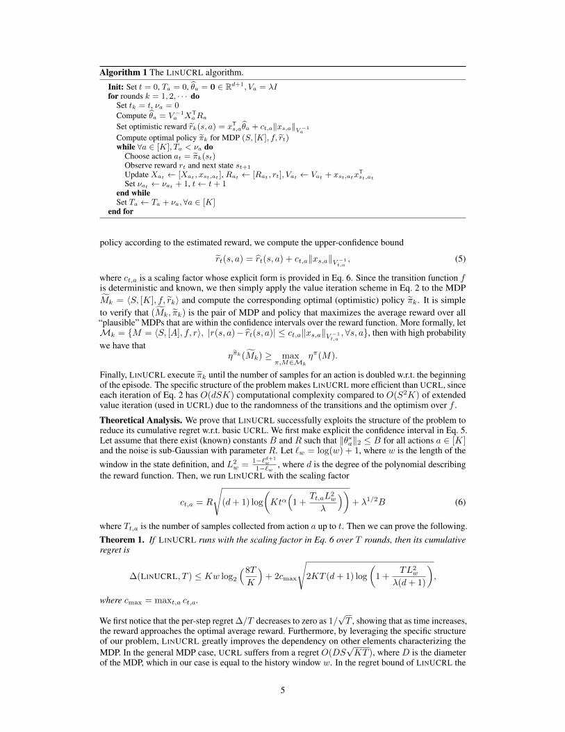
4 Linear Upper-Confidence bound for Reinforcement LearningThe Learning Algorithm. LINUCRL directly builds on the UCRL algorithm [10] and exploits thelinear structure of the reward function and the deterministic and known transition function f . Thecore idea of LINUCRL is to construct confidence intervals on the reward function and apply theoptimism-in-face-of-uncertainty principle to compute an optimistic policy. The structure of LINUCRLis illustrated in Alg. 1. Let us consider an episode k starting at time t, LINUCRL first uses thecurrent samples collected for each action a separately to compute an estimate θ̂t,a by regularizedleast squares, i.e.,

θ̂t,a = minθ

∑τ<t:aτ=a

(xTsτ ,aθ − rτ

)2+ λ‖θ‖2, (4)

where xsτ ,a is the context vector corresponding to state sτ and rτ is the (noisy) reward observedat time τ . Let be Ra,t the vector of rewards obtained up to time t when a was executed and Xa,t

the feature matrix corresponding to the contexts observed so far, then Vt,a =(XTt,aXt,a + λI

)∈

R(d+1)×(d+1) is the design matrix. The closed-form solution of the estimate is θ̂t,a = V −1t,a XTt,aRt,a,

which gives an estimated reward function r̂t(s, a) = xTs,aθ̂t,a. Instead of computing the optimal

4See Sect. 5 for further discussion on the difficulty of finding suitable datasets for the validation of time-varying models.

5In the movielens dataset a timestamp does not correspond to the moment the user saw the movie but whenthe rating is actually submitted. Yet, this does not cancel potential dependencies of future rewards on pastactions.

4

Algorithm 1 The LINUCRL algorithm.

Init: Set t = 0, Ta = 0, θ̂a = 0 ∈ Rd+1, Va = λIfor rounds k = 1, 2, · · · do

Set tk = t, νa = 0Compute θ̂a = V −1

a XTaRa

Set optimistic reward r̃k(s, a) = xTs,aθ̂a + ct,a‖xs,a‖V−1a

Compute optimal policy π̃k for MDP (S, [K], f, r̃t)while ∀a ∈ [K], Ta < νa do

Choose action at = π̃k(st)Observe reward rt and next state st+1

Update Xat ← [Xat , xst,at ], Rat ← [Rat , rt], Vat ← Vat + xst,atxTst,at

Set νat ← νat + 1, t← t+ 1end whileSet Ta ← Ta + νa,∀a ∈ [K]

end for

policy according to the estimated reward, we compute the upper-confidence bound

r̃t(s, a) = r̂t(s, a) + ct,a‖xs,a‖V −1t,a, (5)

where ct,a is a scaling factor whose explicit form is provided in Eq. 6. Since the transition function fis deterministic and known, we then simply apply the value iteration scheme in Eq. 2 to the MDPM̃k = 〈S, [K], f, r̃k〉 and compute the corresponding optimal (optimistic) policy π̃k. It is simpleto verify that (M̃k, π̃k) is the pair of MDP and policy that maximizes the average reward over all“plausible” MDPs that are within the confidence intervals over the reward function. More formally, letMk = {M = 〈S, [A], f, r〉, |r(s, a)− r̂t(s, a)| ≤ ct,a‖xs,a‖V −1

t,a,∀s, a}, then with high probability

we have thatηπ̃k(M̃k) ≥ max

π,M∈Mk

ηπ(M).

Finally, LINUCRL execute π̃k until the number of samples for an action is doubled w.r.t. the beginningof the episode. The specific structure of the problem makes LINUCRL more efficient than UCRL, sinceeach iteration of Eq. 2 has O(dSK) computational complexity compared to O(S2K) of extendedvalue iteration (used in UCRL) due to the randomness of the transitions and the optimism over f .

Theoretical Analysis. We prove that LINUCRL successfully exploits the structure of the problem toreduce its cumulative regret w.r.t. basic UCRL. We first make explicit the confidence interval in Eq. 5.Let assume that there exist (known) constants B and R such that ‖θ∗a‖2 ≤ B for all actions a ∈ [K]and the noise is sub-Gaussian with parameter R. Let `w = log(w) + 1, where w is the length of the

window in the state definition, and L2w =

1−`d+1w

1−`w , where d is the degree of the polynomial describingthe reward function. Then, we run LINUCRL with the scaling factor

ct,a = R

√(d+ 1) log

(Ktα

(1 +

Tt,aL2w

λ

))+ λ1/2B (6)

where Tt,a is the number of samples collected from action a up to t. Then we can prove the following.Theorem 1. If LINUCRL runs with the scaling factor in Eq. 6 over T rounds, then its cumulativeregret is

∆(LINUCRL, T ) ≤ Kw log2

(8T

K

)+ 2cmax

√2KT (d+ 1) log

(1 +

TL2w

λ(d+ 1)

),

where cmax = maxt,a ct,a.

We first notice that the per-step regret ∆/T decreases to zero as 1/√T , showing that as time increases,

the reward approaches the optimal average reward. Furthermore, by leveraging the specific structureof our problem, LINUCRL greatly improves the dependency on other elements characterizing theMDP. In the general MDP case, UCRL suffers from a regret O(DS

√KT ), where D is the diameter

of the MDP, which in our case is equal to the history window w. In the regret bound of LINUCRL the

5

0 10 20 30 40 50 60

1

2

optimal policy

0 10 20 30 40 50 60

1

2

greedy policy

optimal policy

greedypolicy

bestsingle arm

0.1

0.2

0.3

0.4

0.5

0 10 20 30 40 50 60

1

2

optimal policy

0 10 20 30 40 50 60

1

2

greedy policy

optimal policy

greedypolicy

bestsingle arm

0.46

0.48

0.50

0.52

(a) sequence of actions (b) average reward (c) sequence of actions (d) average reward

Figure 2: Optimal policy vs. greedy and fixed-action. The fixed-action policy selects the action with the largest“constant” reward (i.e., ignoring the effects of the recommendation). The greedy policy selects the action with thehighest immediate reward (depending on the state). The optimal policy is computed with value iteration. (a-b):parameters c1 = 0.3, c2 = 0.4, α = 1.5 (limited boredom effect). (c-d): parameters c1 = 2, c2 = 0.01, α = 2(strong boredom effect).

dependency on the number of states (which is exponential in the history window S = Kw) disappearsand it is replaced by the number of parameters d+ 1 in the reward model. Furthermore, since thedynamics is deterministic and known, the only dependency on the diameter w is in a lower-orderlogarithmic term. This result suggests that we can take a large window w and a complex polynomialexpression for the reward (i.e., large d) without compromising the overall regret. Let note that inMDPs, the worst-case regret lower bound also exhibits a

√(T ) dependency ([10]), so there is not

much hope to improve it. The interesting part of these bounds is actually in the problem-specific terms.Furthermore, LINUCRL compares favorably with a linear bandit approach. First, η∗ is in generalmuch larger than the optimal average reward of a greedy policy selecting the best instantanous actionat each step. Second, apart from the log(T ) term, the regret is the same of a linear bandit algorithm(e.g., LINUCB). This means that LINUCRL approaches a better target performance η∗ almost at thesame speed as linear bandit algorithms reach a worse greedy policy. Finally, [19] developed a specificinstance of UCRL for deterministic MDPs, whose final regret is of order O(λA log(T )/∆), where λis the length of the largest simple cycle that can be generated in the MDP and ∆ is the gap betweenthe reward of the optimal and second-optimal policy. While the regret in this bound only scalesas O(log T ), in our setting λ can be as large as S = Kw, which is exponentially worse than thediameter w, and ∆ can be arbitrarily small, thus making a O(

√T ) bound often preferable. We leave

the integration of our linear reward assumption into the algorithm proposed by [19] as future work.

5 Experiments

In order to validate our model on real datasets, we need persistent information about a user iden-tification number to follow the user through time and evaluate how preferences evolve over timein response to the recommendations. This also requires datasets where several RSs are used forthe same user with different cadence and for which it is possible to associate a user-item feedbackwith the system that actually performed that recommendation. Unfortunately, these requirementsmake most of publicly available datasets not suitable for this validation. As a result, we propose touse both synthetic and dataset-based experiments to empirically validate our model and compareLINUCRL to existing baselines. We consider three different scenarios. Toy experiment: A simulatedenvironment with two actions and different parameters, with the objective of illustrating when theoptimal policy could outperform fixed-action and greedy strategies. Movielens: We derive modelparameters from the movielens dataset and we compare the learning performance (i.e., cumulativereward) of LINUCRL to baseline algorithms. Real-world data from A/B testing: this dataset providesenough information to test our algorithm and although our model assumptions are no longer satisfied,we can still investigate how a long-term policy alternating A and B on the basis of past choices canoutperform each solution individually.

Optimal vs. fixed-action and greedy policy. We first illustrate the potential improvement comingfrom a non-static policy that takes into consideration the recent sequence of actions and maximizesthe long-term reward, compared to a greedy policy that selects the action with the higher immediatereward at each step. Intuitively, the gap may be large whenever an action has a large instantaneousreward that decreases very fast as it is selected (e.g., boredom effect). A long-term strategy mayprefer to stick to selecting a sub-optimal action for a while, until the better action goes back to its

6

0 5 10 15 20 25 30 35 40Action

ComedyAdventure

ThrillerDrama

ChildrenCrimeHorror

SciFiAnimation oracle greedy

0 5 10 15 20 25 30 35 40Action

ComedyAdventure

ThrillerDrama

ChildrenCrimeHorror

SciFiAnimation linUCRL

0 5 10 15 20 25 30 35 40Action

ComedyAdventure

ThrillerDrama

ChildrenCrimeHorror

SciFiAnimation linUCB

0 5 10 15 20 25 30 35 40Action

ComedyAdventure

ThrillerDrama

ChildrenCrimeHorror

SciFiAnimation oracle optimal

linUCB UCRL linUCRL oracle greedy

oracle optimal

3.1

3.2

3.3

3.4

3.5

3.6

3.284 3.33 3.486 3.538 3.551

UCRL linUCB oracle greedy

linUCRL oracle optimal

3.20

3.25

3.30

3.35

3.40

3.45

3.50

3.55

3.60

3.327 3.43 3.536 3.54 3.555

(a) Last 40 actions (b) Avg. rwd. at T = 200 (c) Avg. rwd. at the endFigure 3: Results of learning experiment based on movielens dataset.

initial value. We consider the simple case K = 2 and d = 1. Let θ∗1 = (1, c1), θ∗2 = (1/α, c2).We study the optimal policy maximizing the average reward η, a greedy policy that always selectsat = arg maxa r(st, a), and a fixed-action policy at = arg max{1, 1/α}. We first set c1 = 0.3 ≈c2 = 0.4 and α = 1.5, for which the “boredom” effect (i.e., the decrease in reward) is very mild. Inthis case (see Fig. 2-(left)), the fixed-action policy performs very poorly, while greedy and optimalpolicy smartly alternates between actions so as to avoid decreasing the reward of the “best” actiontoo much. In this case, the difference between greedy and optimal policy is very narrow. However inFig. 2-(right), with c1 = 2� c2 = 0.01 and α = 2, we see that the greedy policy switches to action1 too soon to gain immediate reward (plays action 1 for 66% of the time) whereas the optimal policystick to action 2 longer (plays action 1 for 57% of the time) so as to allow action 1 to regain rewardand then go back to select it again. As a result, the optimal policy exploits the full potential of action1 better and eventually gains higher average reward. While here we only illustrate the “boredom”effect (i.e., the reward linearly decreases with the recency), we can imagine a large range of scenarioswhere the greedy policy is highly suboptimal compared to the optimal policy.

Learning on movielens dataset. In order to overcome the difficulty of creating full complex RSand evaluate them on offline datasets, we focus on a relatively simple scenario where a RS directlyrecommends movies from one chosen genre, for which we have already validated our model inSec. 3. One strategy could be to apply a bandit algorithm to find the optimal genre and then alwaysrecommend movies of this genre. On the other hand, our algorithm tries to identify an optimalsequence of those genres to keep the user interested. The standard offline evaluation of a learningalgorithm on historical data is to use a replay or counterfactual strategy [18, 24], which consists inupdating the model whenever the learning algorithm takes the same action as in the logged data,and only update the state (but not the model) otherwise. In our case this replay strategy cannot beapplied because the reward depends on the history of selected actions and we could not evaluatethe reward of an action if the algorithm generated a sequence that is not available in the dataset(which is quite likely). Thus in order to compare the learning performance of LINUCRL to existingbaselines, we use the movielens100k dataset to estimate the parameters of our model and constructthe corresponding “simulator”. Unlike a fully synthetic experiment, this gives a configuration whichis “likely” to appear in practice, as the parameters are directly estimated from real data. We chooseK = 10 actions corresponding to different genres of movies, and we set d = 5 and w = 5, whichresults into Kw = 105 states. We recall that w has a mild impact on the learning performance ofLINUCRL as it does not need to repeatedly try the same action in each state (as UCRL) to be ableto estimate its reward. This is also confirmed by the regret analysis that shows that the regret onlydepends on w in the lower-order logarithmic term of the regret. Given this number of states, UCRLwould need at least one million iteration to observe each state 10 times which is dramatically too largefor the application we consider. The parameters that describe the dependency of the reward functionon the recency (i.e., θ∗j,a) are computed by using the ratings averaged over all users for each stateencountered and for ten different genres in the dataset. The first component of the vectors θ∗a is chosento simulate different user’s preferences and to create complex dynamics in the reward functions. Theresulting parameters and reward functions are reported in App. B. Finally, the observed reward isobtained by adding a small random Gaussian noise to the linear function. In this setting, a constantstrategy would always pull the comedy genre since it is the one with the highest “static” reward,while other genres are also highly rewarding and a suitable alternation between them may provide amuch higher reward.

We compare LINUCRL to the following algorithms: oracle optimal (π∗), oracle greedy (greedycontextual policy), LINUCB [1] (learn the parameters using LINUCB for each action and select the

7

Algorithm on the T steps on the last stepsonly B 46.0% 46.0%UCRL 46.5% 46.0%

LINUCRL 66.7% 75.8%oracle greedy 61.3% 61.3%oracle optimal 95.2% 95.2%

Table 2: Relative improvement over only A of learning experiment based on large scale A/B testingdataset.

one with largest instantaneous reward), UCRL [3] (considering each action and state independently).The results are obtained by averaging 4 independent runs. Fig. 3(b-c) shows the average reward atT = 200 and after T = 2000 steps. We first notice that as in the previous experiment the oraclegreedy policy is suboptimal compared to the optimal policy that maximizes the long-term reward.Despite the fact that UCRL targets this better performance, the learning process is very slow as thenumber of states is too large. Indeed this number of steps is lower than the number of states so UCRLdid not have the chance to update its policy since in average no states has been visited twice. On theother hand, at early learning stages LINUCRL is already better than LINUCB, and its performancekeeps improving until, at 2000 steps, it actually performs better than the oracle greedy strategy and itis close to the optimal policy.

Large scale A/B testing dataset. We also validate our approach on a real-world A/B testing dataset.We collected 15 days of click on ads history of a CRITEO’s test, where users have been proposed twovariations on the display denoted as A and B. Each display is actually the output of two real-worldcollaborative-filtering recommender strategies; precise information on how these algorithms areconstructed is not relevant for our analysis. Unlike a classical A/B testing each unique user hasbeen exposed to both A and B but with different frequencies. This dataset is formed of 350Mtuples (user id, timestamp, version, click) and will be released publicly as soon as possible. Remarkthat the system is already heavily optimized and that even a small improvement in the click-rate isvery desirable. As in the movielens experiment, we do not have enough data to evaluate a learningalgorithm on the historical events (not enough samples per state would be available), so we firstcompute a simulator based on the data and then run LINUCRL- that does not know the parameters ofthe simulator and must try to estimate them - and compare it to simple baselines. Unlike the previousexperiment, we do not impose any linear assumption on the simulator (as in Eq. 1) and we computethe click probability for actions A and B independently in each state (we set w = 10, for a totalof 210 = 1024 states) and whenever that state-action pair is executed we draw a Bernoulli with thecorresponding probability. Using this simulator we compute oracle greedy and optimal policies andwe compare LINUCB, LINUCRL, which is no longer able to learn the “true” model, since it doesnot satisfy the linear assumption, and UCRL, which may suffer from the large number of state buttargets a model with potentially better performance (as it can correctly estimate the actual rewardfunction and not just a linear approximation of it). We report the results (averaged over 5 runs) asa relative improvement over the worst fixed option (i.e., in this case A). Tab. 2 shows the averagereward over T = 2, 000 steps and of the learned policy at the end of the experiment. Despite the factthat the simulator does not satisfy our modeling assumptions, LINUCRL is still the most competitivealgorithm as it achieves the best performance among the learning algorithms and it outperforms theoracle greedy policy.

6 Conclusion

We showed that estimating the influence of the recommendation strategy on the reward and computinga policy maximizing the long-term reward may significantly outperform fixed-action or greedycontextual policies. We introduced a novel learning algorithm, LINUCRL, to effectively learn suchpolicy and we prove that its regret is much smaller than for standard reinforcement learning algorithms(UCRL). We validated our model and its usefulness on the movielens dataset and on a novel A/B testingdataset. Our results illustrate how the optimal policy effectively alternates between different options,in order to keep the interest of the users as high as possible. Furthermore, we compared LINUCRLto a series of learning baselines on simulators satisfying our linearity assumptions (movielens) ornot (A/B testing). A venue for future work is to extend the current model to take into considerationcorrelations between actions. Furthermore, given its speed of convergence, it could be interestingto run a different instance of LINUCRL per user - or group of users - in order to offer personalized“boredom” curves. Finally, using different models of the reward as a function of the recency (e.g.,logistic regression) could be used in case of binary rewards.

8

References[1] Y. Abbasi-yadkori, D. Pál, and C. Szepesvári. Improved algorithms for linear stochastic bandits.

In J. Shawe-Taylor, R. S. Zemel, P. L. Bartlett, F. Pereira, and K. Q. Weinberger, editors,Advances in Neural Information Processing Systems 24, pages 2312–2320. Curran Associates,Inc., 2011.

[2] P. Auer. Using confidence bounds for exploitation-exploration trade-offs. J. Mach. Learn. Res.,3:397–422, mar 2003.

[3] P. Auer, T. Jaksch, and R. Ortner. Near-optimal regret bounds for reinforcement learning. InD. Koller, D. Schuurmans, Y. Bengio, and L. Bottou, editors, Advances in Neural InformationProcessing Systems 21, pages 89–96. Curran Associates, Inc., 2009.

[4] S. Bubeck and N. Cesa-Bianchi. Regret analysis of stochastic and nonstochastic multi-armedbandit problems. Foundations and Trends R© in Machine Learning, 5(1):1–122, 2012.

[5] A. Dasdan, S. S. Irani, and R. K. Gupta. Efficient algorithms for optimum cycle mean andoptimum cost to time ratio problems. In Proceedings of the 36th Annual ACM/IEEE DesignAutomation Conference, DAC ’99, pages 37–42, New York, NY, USA, 1999. ACM.

[6] S. Filippi, O. Cappé, and A. Garivier. Optimally Sensing a Single Channel Without PriorInformation: The Tiling Algorithm and Regret Bounds. IEEE Journal of Selected Topics inSignal Processing, 5(1):68 – 76, Feb. 2010.

[7] F. M. Harper and J. A. Konstan. The movielens datasets: History and context. ACM Trans.Interact. Intell. Syst., 5(4):19:1–19:19, Dec. 2015.

[8] H. Heidari, M. Kearns, and A. Roth. Tight policy regret bounds for improving and decay-ing bandits. In Proceedings of the Twenty-Fifth International Joint Conference on ArtificialIntelligence, IJCAI’16, pages 1562–1570. AAAI Press, 2016.

[9] J. Herlocker, J. Konstan, A. Borchers, and J. Riedl. An algorithmic framework for performingcollaborative filtering. In Proceedings of the 1999 Conference on Research and Development inInformation Retrieval, 1999.

[10] T. Jaksch, R. Ortner, and P. Auer. Near-optimal regret bounds for reinforcement learning. J.Mach. Learn. Res., 11:1563–1600, Aug. 2010.

[11] K. G. Jamieson and A. Talwalkar. Non-stochastic best arm identification and hyperparameteroptimization. In AISTATS, 2016.

[12] K. Kapoor, K. Subbian, J. Srivastava, and P. Schrater. Just in time recommendations: Modelingthe dynamics of boredom in activity streams. In Proceedings of the Eighth ACM InternationalConference on Web Search and Data Mining, WSDM ’15, pages 233–242, New York, NY, USA,2015. ACM.

[13] R. M. Karp. A characterization of the minimum cycle mean in a digraph. 23:309–311, 12 1978.

[14] J. Komiyama and T. Qin. Time-Decaying Bandits for Non-stationary Systems, pages 460–466.Springer International Publishing, Cham, 2014.

[15] Y. Koren. Collaborative filtering with temporal dynamics. In Proceedings of the 15th ACMSIGKDD International Conference on Knowledge Discovery and Data Mining, KDD ’09, pages447–456, New York, NY, USA, 2009. ACM.

[16] Y. Koren, R. Bell, and C. Volinsky. Matrix factorization techniques for recommender systems.Computer, 42(8):30–37, Aug. 2009.

[17] L. Li, W. Chu, J. Langford, and R. E. Schapire. A contextual-bandit approach to personalizednews article recommendation. In M. Rappa, P. Jones, J. Freire, and S. Chakrabarti, editors,WWW, pages 661–670. ACM, 2010.

9

[18] L. Li, W. Chu, J. Langford, and X. Wang. Unbiased offline evaluation of contextual-bandit-basednews article recommendation algorithms. In Proceedings of the Fourth ACM InternationalConference on Web Search and Data Mining, WSDM ’11, pages 297–306, New York, NY, USA,2011. ACM.

[19] R. Ortner. Online regret bounds for markov decision processes with deterministic transitions. InY. Freund, L. Györfi, G. Turán, and T. Zeugmann, editors, Algorithmic Learning Theory, pages123–137, Berlin, Heidelberg, 2008. Springer Berlin Heidelberg.

[20] R. Ortner, D. Ryabko, P. Auer, and R. Munos. Regret bounds for restless markov bandits. Theor.Comput. Sci., 558:62–76, 2014.

[21] G. Shani, D. Heckerman, and R. I. Brafman. An mdp-based recommender system. J. Mach.Learn. Res., 6:1265–1295, Dec. 2005.

[22] M. Soare, A. Lazaric, and R. Munos. Best-Arm Identification in Linear Bandits. In NIPS -Advances in Neural Information Processing Systems 27, Montreal, Canada, Dec. 2014.

[23] R. S. Sutton and A. G. Barto. Introduction to Reinforcement Learning. MIT Press, Cambridge,MA, USA, 1st edition, 1998.

[24] A. Swaminathan and T. Joachims. Batch learning from logged bandit feedback throughcounterfactual risk minimization. J. Mach. Learn. Res., 16(1):1731–1755, Jan. 2015.

[25] C. Tekin and M. Liu. Online Learning of Rested and Restless Bandits. IEEE Transactions onInformation Theory 58(8), Aug. 2012.

10

A Proof of Theorem 1

Proof. In order to prove Thm. 1, we first need the following proposition about the confidence intervalsused in computing the optimistic reward r̃(s, a).

Proposition 2. Let assume ‖θ∗a‖2 ≤ B. If θ̂t,a is computed as in Eq. 4 and ct,a is defined as in Eq. 6,then

P(r(s, a) ≤ r̂(s, a) + ct,a‖xs,a‖V −1

t,a

)≤ t−α

K.

Proof. By definition of ρ(s, a) we have 0 ≤ ρ(s, a) ≤∑wτ=1

1τ< log(w) + 1

.= `w. Thus 1 ≤ ‖xs,a‖22 ≤∑d

j=0 `jw =

1−`d+1w

1−`w = L2w. Using Thm. 2 of [1], we have with probability 1− δ,

‖θ̂t,a − θ∗a‖Vt,a ≤ R

√(d+ 1) log

(1 + Tt,aL2

w/λ

δ

)+ λ1/2B.

Thus for all s ∈ S we have,

|r(s, a)− r̂(s, a)| = |xTs,aθ̂t,a − xTs,aθ∗a| ≤ ‖xs,a‖V−1t,a‖θ̂a − θ∗a‖Vt,a .

Using δ = t−α

Kconcludes the proof.

An immediate result of Prop. 2 is that the estimated average reward of π̃k in the optimistic MDP M̃k

is an upper-confidence bound on the optimal average reward, i.e., for any t (the probability followsby a union bound over actions)

P(η∗ > ηπ̃k(M̃k)

)≤ t−α. (7)

We are now ready to prove the main result.

Proof of Thm. 1. We follow similar steps as in [10]. We split the regret over episodes as

∆(A, T ) =

m∑k=1

tk+1−1∑t=tk

(η∗ − r(st, at)

)=

m∑k=1

∆k.

Let Tk,a = {tk ≤ t < tk+1 : at = a} be the steps when action a is selected during episode k. Weupper bound the per-episode regret as

∆k =∑a∈[K]

∑t∈Tk,a

(η∗ − r(st, a)

)≤tk+1−1∑t=tk

(η̃k − r̃k(st, a)

)+∑a∈[K]

∑t∈Tk,a

(r̃k(st, a)− r(st, a)

),

where the inequality directly follows from the event that η̃k ≥ η∗ (Eq. 7) with probability 1− T−α.Notice that the low-probability event of failing confidence intervals can be treated as in [10].

We proceed by bounding the first term of Eq. 8. Unlike in the general online learning scenario, inour setting the transition function f is known and thus the regret incurred from bad estimates of thedynamics is reduced to zero. Furthermore, since we are dealing with deterministic MDPs, the optimalpolicy converges to a loop over states. When starting a new policy, we may start from a state outsideits loop. Nonetheless, it is easy to verify that starting from any state s, it is always possible to reachany desired state s′ in at most w steps (i.e., the size of the history window). As a result, within eachepisode k the difference between the cumulative reward (

∑t r̃k(st, a)) and the (optimistic) average

reward ((tk+1 − tk)η̃k) in the loop never exceeds w. Furthermore, since episodes terminate whenone action doubles its number of samples, using a similar proof as [10], we have that the number ofepisodes is bounded as m ≤ K log2( 8T

K ). As a result, the contribution of the first term of Eq. 8 to theoverall regret is bounded as

m∑k=1

tk+1−1∑t=tk

(η̃k − r̃k(st, a)

)≤ Kw log2

(8T

K

). (8)

11

The second term in Eq. 8 refers to the (cumulative) reward estimation error and it can be decomposedas

|r̃k(st, a)− r(st, a)| ≤ |r̃k(st, a)− r̂k(st, a)|+ |r̂k(st, a)− r(st, a)|.

We can bound the cumulative sum of the second term as (similar for the first, since r̃k belongs to theconfidence interval of r̂k by construction)

m∑k=1

∑a∈[K]

∑t∈Tk,a

|r̂k(st, a)− r(st, a)| ≤m∑k=1

∑a∈[K]

∑t∈Tk,a

ct,a‖xst,a‖V−1a,t

≤ cmax

∑a∈[K]

√√√√ m∑k=1

∑t∈Tk,a

‖xst,a‖2V−1a,t

√Ta,

where the first inequality follows from Prop. 2 with probability 1− T−α, and Ta is the total numberof times a has been selected at step T . Let Ta = ∪kTk,a, then using Lemma 11 of [1], we have∑

t∈Ta

‖xst,a||2V −1t,a≤ 2 log

det(VT,a)

det(λI),

and by Lem. 10 of [1], we have

det(Vt,a) ≤ (λ+ tL2w/(d+ 1))d+1,

which leads tom∑k=1

∑a∈[K]

∑t∈Tk,a

|r̂k(st, a)− r(st, a)| ≤ cmax

∑a∈[K]

√Ta

√2(d+ 1) log

( λ+ tL2w

λ(d+ 1)

)

≤ cmax

√2KT (d+ 1) log

( λ+ tL2w

λ(d+ 1)

).

Bringing all the terms together gives the regret bound.

B Experiments Details

Genre θ∗a,0 θ∗a,1 θ∗a,2 θ∗a,3 θ∗a,4 θ∗a,5Action 3.1 0.54 -1.08 0.78 -0.22 0.02

Comedy 3.34 0.54 -1.08 0.78 -0.22 0.02Adventure 3.51 0.86 -2.7 3.06 -1.46 0.24Thriller 3.4 1.26 -2.9 2.76 -1.14 0.16Drama 2.75 1.0 0.94 -1.86 0.94 -0.16

Children 3.52 0.1 0.0 -0.3 0.2 -0.04Crime 3.37 0.32 1.12 -3.0 2.26 -0.54Horror 3.54 -0.68 1.84 -2.04 0.82 -0.12SciFi 3.3 0.64 -1.32 1.1 -0.38 0.02

Animation 3.4 1.38 -3.44 3.62 -1.62 0.24Table 3: Reward parameters of each genre for the movielens experiment.

The parameters used in the MovieLens experiment are reported in Table 3.

12