features and matching - courses.cs.washington.edu

Features and MatchingCSE P576

Vitaly Ablavsky

These slides were developed by Dr. Matthew Brown for CSEP576 Spring 2020 and adapted (slightly) for Fall 2021 credit → Matt blame → Vitaly

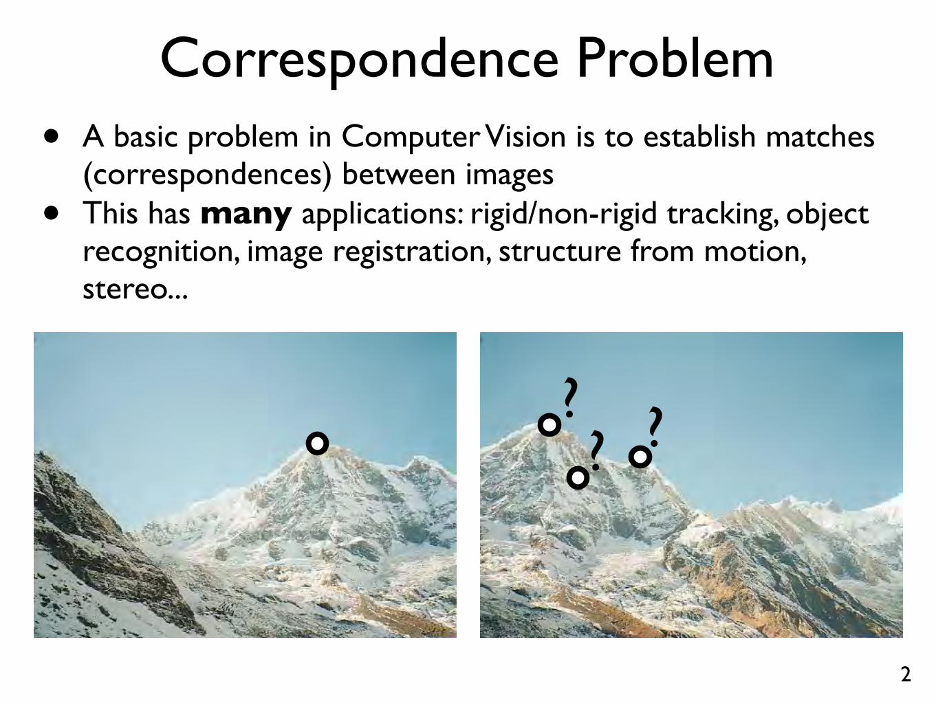
Correspondence Problem• A basic problem in Computer Vision is to establish matches

(correspondences) between images

• This has many applications: rigid/non-rigid tracking, objectrecognition, image registration, structure from motion, stereo...

2

? ??

Feature Detectors

3

206 Computer Vision: Algorithms and Applications (September 3, 2010 draft)

(a) (b)

(c) (d)

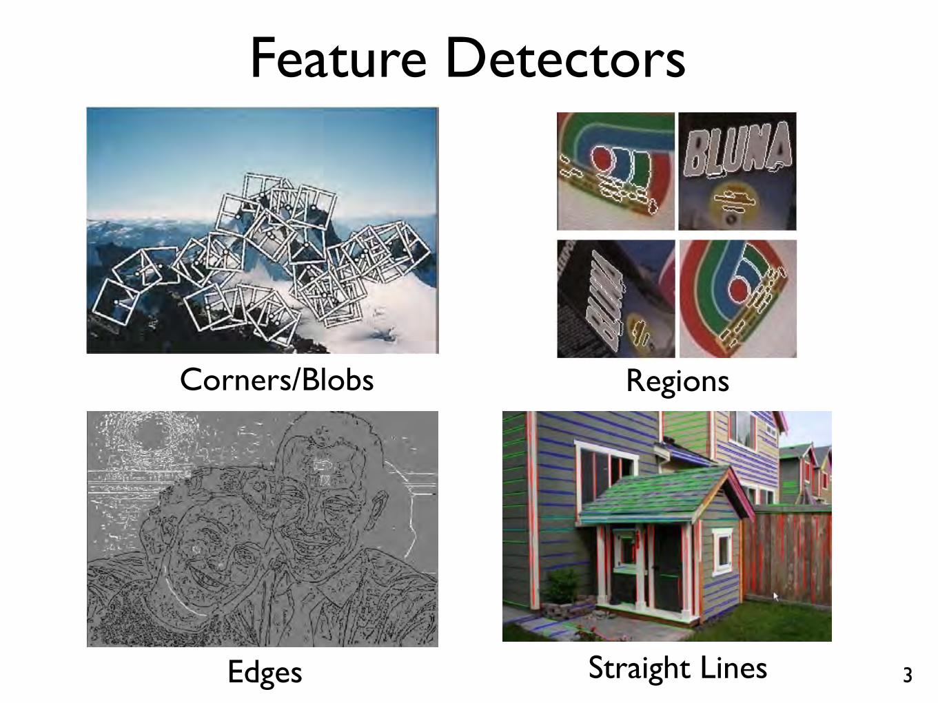
Figure 4.1 A variety of feature detectors and descriptors can be used to analyze, describe andmatch images: (a) point-like interest operators (Brown, Szeliski, and Winder 2005) c 2005IEEE; (b) region-like interest operators (Matas, Chum, Urban et al. 2004) c 2004 Elsevier;(c) edges (Elder and Goldberg 2001) c 2001 IEEE; (d) straight lines (Sinha, Steedly, Szeliskiet al. 2008) c 2008 ACM.


(a) (b)

(c) (d)



(a) (b)

(c) (d)



(a) (b)

(c) (d)


Corners/Blobs Regions

Edges Straight Lines

Feature Descriptors

4

Preprocessing

Conv0

Pool0

Conv1

Pool1Metric network

Cross-Entropy Loss

Sampling

Conv2

Conv3

Conv4

Bottleneck

Pool4 FC2

FC1

FC3 + Softmax

A: Feature network B: Metric network

C: MatchNet in training

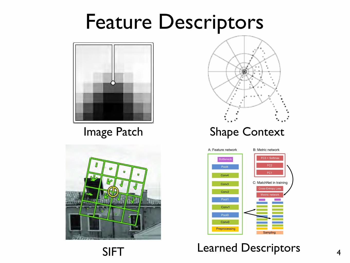
Figure 1. The MatchNet architecture. A: The feature network usedfor feature encoding, with an optional bottleneck layer to reducefeature dimension. B: The metric network used for feature com-parison. C: In training, the feature net is applied as two “towers”on pairs of patches with shared parameters. Output from the twotowers are concatenated as the metric network’s input. The entirenetwork is jointly trained on labeled patch-pairs generated fromthe sampler to minimize the cross-entropy loss. In prediction, thetwo sub-networks (A and B) are conveniently used in a two-stagepipeline (See Section 4.2).

[0, 1] from the two units of FC3, These are non-negative,sum up to one, and can be interpreted as the network’s es-timate of probability that the two patches match and do notmatch, respectively.

Two-tower structure with tied parameters: The patch-based matching task usually assumes that patches gothrough the same feature encoding before computing a sim-ilarity. Therefore we need just one feature network. Duringtraining, this can be realized by employing two feature net-works (or “towers”) that connect to a comparison network,with the constraint that the two towers share the same pa-rameters. Updates for either tower will be applied to theshared coefficients.

This approach is related to the Siamese network [2, 5],which also uses two towers, but with carefully designedloss functions instead of a learned metric network. A re-cent preprint on learning a network for stereo matching hasalso used the two-tower-plus-fully-connected comparison-network approach [37]. In contrast, MatchNet includesmax-pooling layers to deal with scale changes that are notpresent in stereo reconstruction problems, and it also has

Table 1. Layer parameters of MatchNet. The output dimensionis given by (height ⇥ width ⇥ depth). PS: patch size for con-volution and pooling layers; S: stride. Layer types: C: convo-lution, MP: max-pooling, FC: fully-connected. We always padthe convolution and pooling layers so the output height and widthare those of the input divided by the stride. For FC layers,their size B and F are chosen from: B 2 {64, 128, 256, 512},F 2 {128, 256, 512, 1024}. All convolution and FC layers useReLU activation except for FC3, whose output is normalized withSoftmax (Equation 2).

Name Type Output Dim. PS S

Conv0 C 64⇥ 64⇥ 24 7⇥ 7 1Pool0 MP 32⇥ 32⇥ 24 3⇥ 3 2Conv1 C 32⇥ 32⇥ 64 5⇥ 5 1Pool1 MP 16⇥ 16⇥ 64 3⇥ 3 2Conv2 C 16⇥ 16⇥ 96 3⇥ 3 1Conv3 C 16⇥ 16⇥ 96 3⇥ 3 1Conv4 C 16⇥ 16⇥ 64 3⇥ 3 1Pool4 MP 8⇥ 8⇥ 64 3⇥ 3 2Bottleneck FC B - -

FC1 FC F - -FC2 FC F - -FC3 FC 2 - -

more convolutional layers compared to [37].In other settings, where similarity is defined over patches

from two significantly different domains, the MatchNetframework can be generalized to have two towers that sharefewer layers or towers with different structures.

The bottleneck layer: The bottleneck layer can be usedto reduce the dimension of the feature representation and tocontrol overfitting of the network. It is a fully-connectedlayer of size B, between the 4096 (8 ⇥ 8 ⇥ 64) nodes inthe output of Pool4 and the final output of the feature net-work. We evaluate how B affects matching performance inSection 5 and plot results in Figure 4.

The preprocessing layer: Following a previous conven-tion, for each pixel in the input grayscale patch we normal-ize its intensity value x (in [0, 255]) to (x� 128)/160.

4. Training and predictionThe feature and metric networks are trained jointly in a

supervised setting using a two-tower structure illustrated inFigure 1-C. We minimize the cross-entropy error

E = � 1

n

nX

i=1

[yi log(yi) + (1� yi) log(1� yi)] (1)

over a training set of n patch pairs using stochastic gradientdescent (SGD) with a batch size of 32. Here yi is the 0/1label for input pair xi. 1 indicates match. yi and 1� yi arethe Softmax activations computed on the values of the two

Image Patch

SIFT

Shape Context

Learned Descriptors

Features and Matching• Feature detectors

- Canny edges, Harris corners, DoG, MSERs

• Feature descriptors- Image patches, invariance, SIFT, learned features

5[ Szeliski Chapter 7 ]

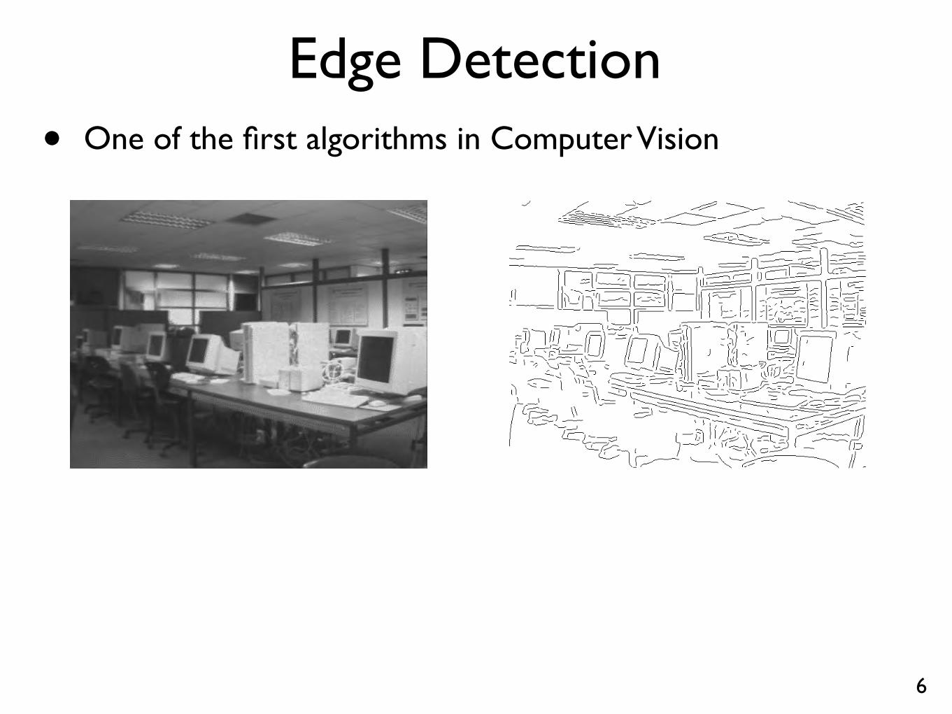
Edge Detection• One of the first algorithms in Computer Vision

6

Introduction 11

Feature extraction

The first stages of most computer vision algorithmsperform feature extraction. The aim is to reducethe data content of the images while preserving theuseful information they contain.

The most commonly used features are edges, whichare detected along 1-dimensional intensity disconti-nuities in the image. Automatic edge detection algo-rithms produce something resembling a line drawingof the scene.

Corner detection is alsocommon. Corner featuresare particularly useful formotion analysis.

Edge Detection• Consider edge detection for a 1D signal

7

6 Engineering Part IIB: 4F12 Feature Extraction

1D edge detection

We start with the simple case of edge detection inone dimension. When developing an edge detec-tion algorithm, it is important to bear in mind theinvariable presence of image noise. Consider thissignal I(x) with an obvious edge.

0 200 400 600 800 1000 1200 1400 1600 1800 2000

Sign

al

An intuitive approach to edge detection might beto look for maxima and minima in I ′(x).

0 200 400 600 800 1000 1200 1400 1600 1800 2000

0

Diff

eren

tiate

d si

gnal

This simple strategy is defeated by noise. For thisreason, all edge detectors start by smoothing thesignal to suppress noise. The most common ap-proach is to use a Gaussian filter.

[ Slide credits: R. Cipolla ]


1D edge detection

We start with the simple case of edge detection inone dimension. When developing an edge detec-tion algorithm, it is important to bear in mind theinvariable presence of image noise. Consider thissignal I(x) with an obvious edge.

0 200 400 600 800 1000 1200 1400 1600 1800 2000

Sign

al

An intuitive approach to edge detection might beto look for maxima and minima in I ′(x).

0 200 400 600 800 1000 1200 1400 1600 1800 2000

0

Diff

eren

tiate

d si

gnal

This simple strategy is defeated by noise. For thisreason, all edge detectors start by smoothing thesignal to suppress noise. The most common ap-proach is to use a Gaussian filter.

• Naive approach: look for maxima/minima in

I(x)

I 0(x)

What’s the problem?

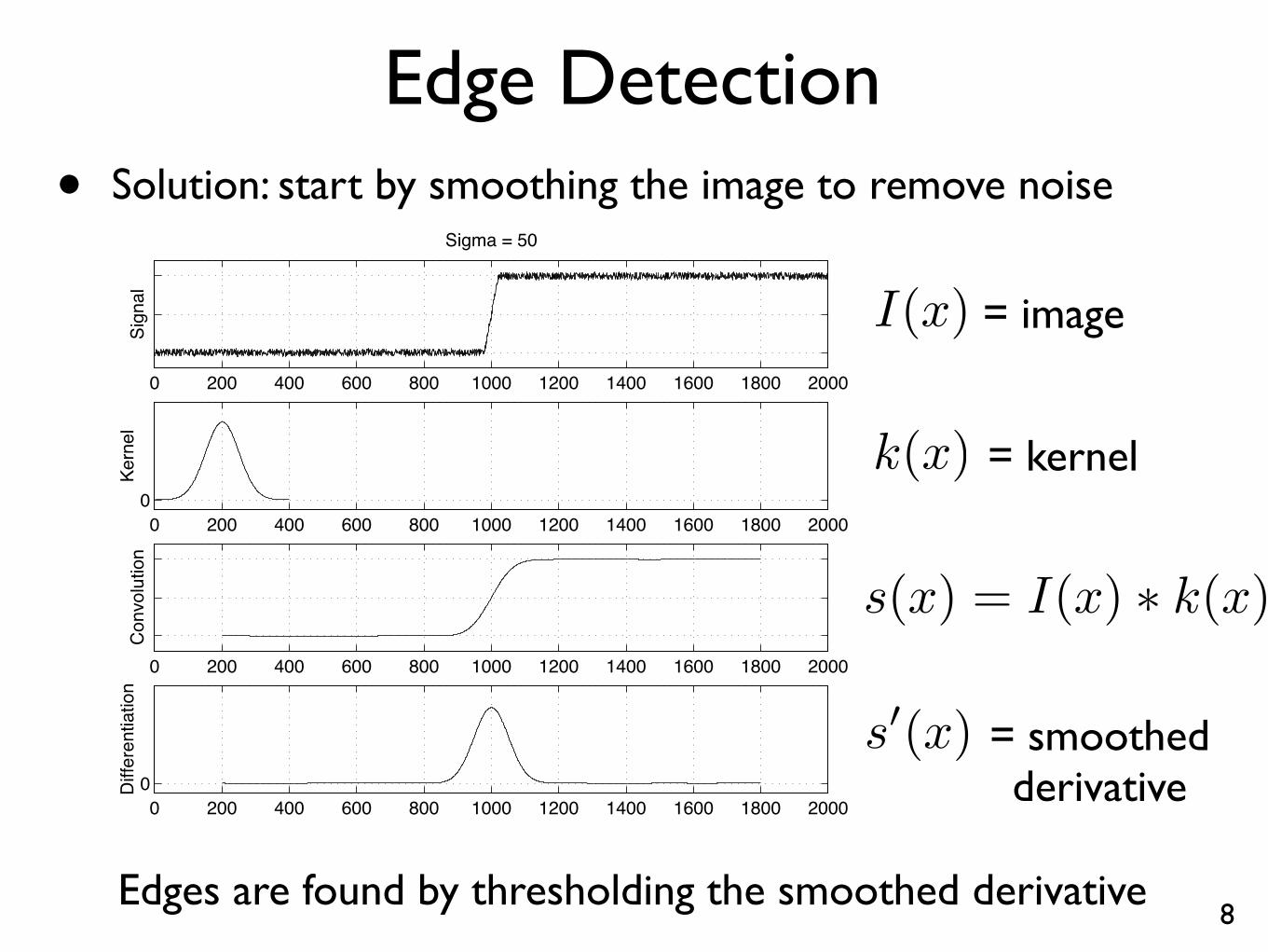
Edge Detection• Solution: start by smoothing the image to remove noise

8

Feature Extraction 7

1D edge detection

A broad overview of 1D edge detection is:

1. Convolve the signal I(x) with a Gaussian kernelgσ(x). Call the smoothed signal s(x).

gσ(x) =1

σ√

2πexp

(

−x2

2σ2

)

2. Compute s′(x), the derivative of s(x).

3. Find maxima and minima of s′(x).

4. Use thresholding on the magnitude of the ex-trema to mark edges.

0 200 400 600 800 1000 1200 1400 1600 1800 2000

Sign

al

Sigma = 50

0 200 400 600 800 1000 1200 1400 1600 1800 20000

Kern

el

0 200 400 600 800 1000 1200 1400 1600 1800 2000

Con

volu

tion

0 200 400 600 800 1000 1200 1400 1600 1800 20000D

iffer

entia

tion

I(x)

k(x)

s(x) = I(x) ⇤ k(x)

s0(x)

= image

= kernel

= smoothedderivative

Edges are found by thresholding the smoothed derivative

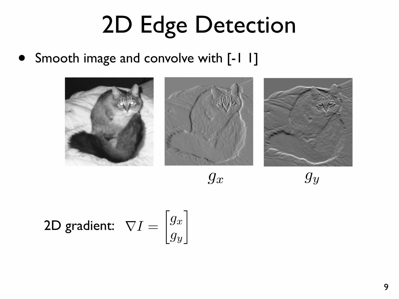
2D Edge Detection• Smooth image and convolve with [-1 1]

9

Image Gradient• Horizontal and vertical gradients

13

12.4


13

12.4


13

12.4

gx gy

rI =

gxgy

�2D gradient:

2D Edge Detection• Look at the magnitude of the smoothed gradient

10


2D edge detection

The next step is to find the gradient of the smoothedimage S(x, y) at every pixel:

∇S = ∇(Gσ ∗ I)

=

∂(Gσ∗I)∂x

∂(Gσ∗I)∂y

=

∂Gσ∂x ∗ I

∂Gσ∂y ∗ I

The following example shows |∇S| for a fruity im-age:

(a) Original image (b) Edge strength |∇S|


2D edge detection


∇S = ∇(Gσ ∗ I)

=

∂(Gσ∗I)∂x

∂(Gσ∗I)∂y

=

∂Gσ∂x ∗ I

∂Gσ∂y ∗ I



• Non-maximal suppression (keep only points where is a maximum in directions )

|rI|

|rI| =qg2x + g2y

|rI|±rI

[ Canny 1986 ]

11


2D edge detection


∇S = ∇(Gσ ∗ I)

=

∂(Gσ∗I)∂x

∂(Gσ∗I)∂y

=

∂Gσ∂x ∗ I

∂Gσ∂y ∗ I




2D edge detection


∇S = ∇(Gσ ∗ I)

=

∂(Gσ∗I)∂x

∂(Gσ∗I)∂y

=

∂Gσ∂x ∗ I

∂Gσ∂y ∗ I



11

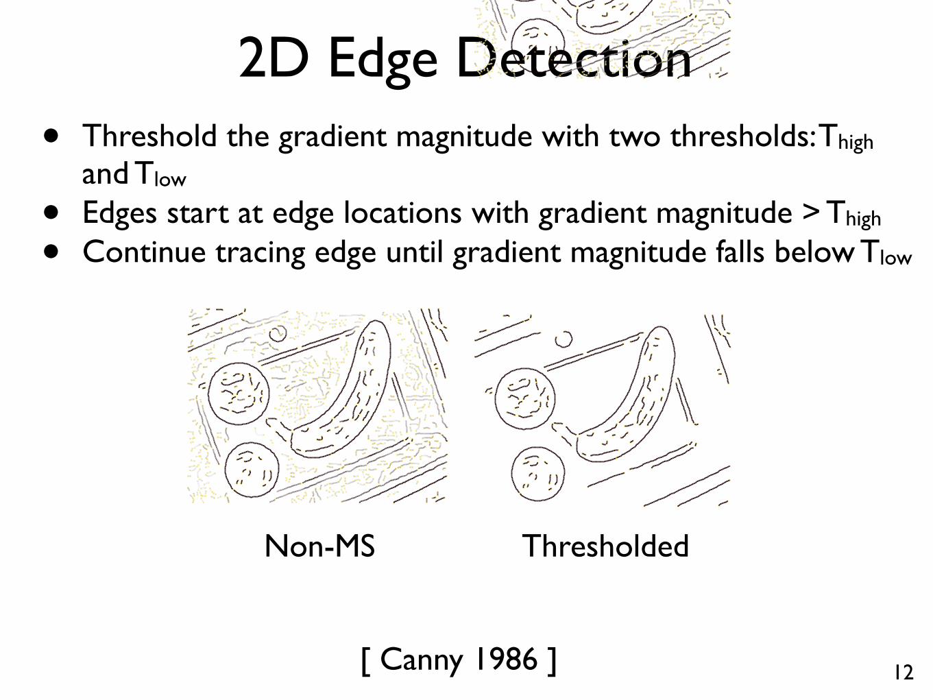
2D Edge Detection• Threshold the gradient magnitude with two thresholds: Thigh

and Tlow

• Edges start at edge locations with gradient magnitude > Thigh

• Continue tracing edge until gradient magnitude falls below Tlow

12


2D edge detection

The next stage of the edge detection algorithmis non-maximal suppression. Edge elements,or edgels, are placed at locations where |∇S| isgreater than local values of |∇S| in the directions±∇S. This aims to ensure that all edgels are lo-cated at ridge-points of the surface |∇S|.

(c) Non-maximal suppression

Next, the edgels are thresholded, so that onlythose with |∇S| above a certain value are retained.

(d) Thresholding


2D edge detection

The next stage of the edge detection algorithmis non-maximal suppression. Edge elements,or edgels, are placed at locations where |∇S| isgreater than local values of |∇S| in the directions±∇S. This aims to ensure that all edgels are lo-cated at ridge-points of the surface |∇S|.

(c) Non-maximal suppression

Next, the edgels are thresholded, so that onlythose with |∇S| above a certain value are retained.

(d) ThresholdingThresholdedNon-MS

[ Canny 1986 ]

Edges + Segmentation• Segmentation is subjective [ Martin, Fowlkes, Tal, Malik 2001 ]

13

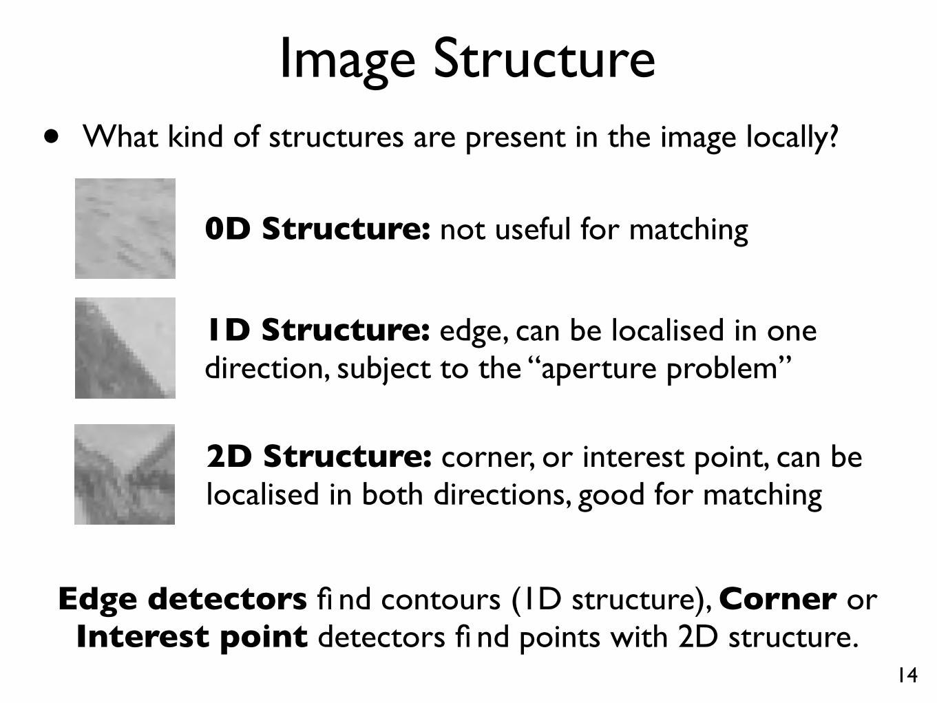
Image Structure• What kind of structures are present in the image locally?

14

0D Structure: not useful for matching

1D Structure: edge, can be localised in one direction, subject to the “aperture problem”

2D Structure: corner, or interest point, can be localised in both directions, good for matching

Edge detectors fi nd contours (1D structure), Corner or Interest point detectors fi nd points with 2D structure.

Local SSD Function• Consider the sum squared difference (SSD) of a patch with

its local neighbourhood

15

�x1

�x2

x =

x1

x2

�

SSD =X

R|I(x)� I(x+�x)|2

Local SSD Function• Consider the local SSD function for different patches

16

4.1 Points and patches 211

(a)

(b) (c) (d)

Figure 4.5 Three auto-correlation surfaces EAC(�u) shown as both grayscale images andsurface plots: (a) The original image is marked with three red crosses to denote where theauto-correlation surfaces were computed; (b) this patch is from the flower bed (good uniqueminimum); (c) this patch is from the roof edge (one-dimensional aperture problem); and (d)this patch is from the cloud (no good peak). Each grid point in figures b–d is one value of�u.


(a)

(b) (c) (d)



(a)

(b) (c) (d)



(a)

(b) (c) (d)



(a)

(b) (c) (d)



(a)

(b) (c) (d)


Clear peak in similarity function

High similarity along the edge

High similarity locally

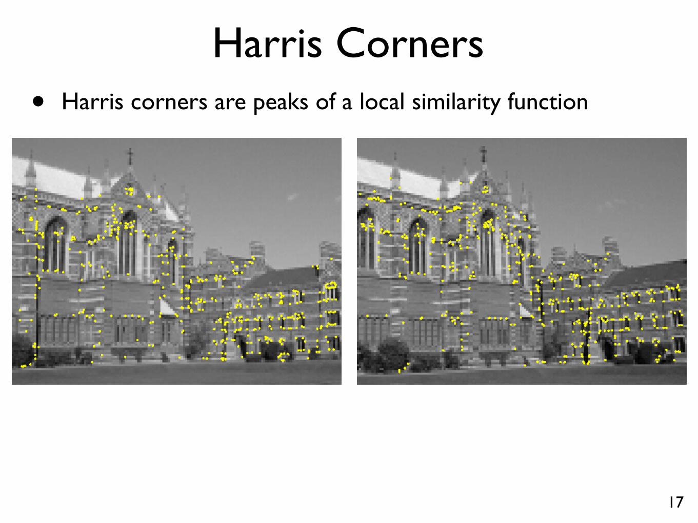
Harris Corners• Harris corners are peaks of a local similarity function

17

Harris Corners• We will use a first order approximation to the local SSD

function

18

�x1

�x2 SSD =X

R|I(x)� I(x+�x)|2

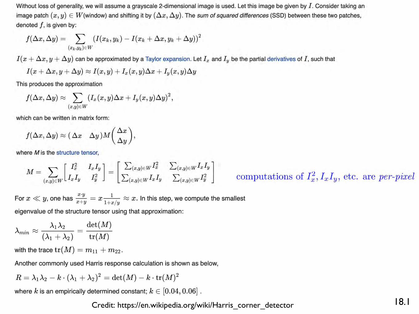
Credit: https://en.wikipedia.org/wiki/Harris_corner_detector 18.1

Harris Corners• Corners matched using correlation

19

99 inliers 89 outliers

[ Zhang, Deriche, Faugeras, Luong 1995, Beardsley, Torr, Zisserman 1996 ]

Difference of Gaussian• DoG = centre-surround filter

20

=⇤

• Find local-maxima of the centre surround response

Non-maximal suppression: These points are maxima

in a 10 pixel radius

Difference of Gaussian• DoG detects blobs at scale that depends on the Gaussian

standard deviation(s)

21

0 5 10 15 20 25 30 35 40 45−0.02

−0.015

−0.01

−0.005

0

0.005

0.01

red = [1 � 2 1] ⇤ g(x; 5.0)black = g(x; 5.0)� g(x; 4.0)

Note: DOG ≈ Laplacian of Gaussian

Detection Scale • Smoothing standard deviations determine scale of detected

features, e.g., edge detection in cloth

22


Multi-scale edge detection

The amount of smoothing controls the scale atwhich we analyse the image. There is no right orwrong size for the Gaussian kernel: it all dependson the scale we’re interested in.

Modest smoothing (a Gaussian kernel with small σ)brings out edges at a fine scale. More smoothing(larger σ) identifies edges at larger scales, suppress-ing the finer detail.

This is an image of a dish cloth.After edge detection, we seedifferent features at differentscales.

σ = 1 σ = 5

Fine scale edge detection is particularly sensitiveto noise. This is less of an issue when analysingimages at coarse scales.






σ = 1 σ = 5







σ = 1 σ = 5


• Many algorithms use multi-scale architectures to get around this problem

• e.g., Scale-Invariant Feature Transform “SIFT”

MSERS• Maximally Stable Extremal Regions

23


Figure 4.15 Maximally stable extremal regions (MSERs) extracted and matched from anumber of images (Matas, Chum, Urban et al. 2004) c 2004 Elsevier.

Figure 4.16 Feature matching: how can we extract local descriptors that are invariantto inter-image variations and yet still discriminative enough to establish correct correspon-dences?

are therefore invariant to both affine geometric and photometric (linear bias-gain or smoothmonotonic) transformations (Figure 4.15). If desired, an affine coordinate frame can be fit toeach detected region using its moment matrix.

The area of feature point detectors continues to be very active, with papers appearing ev-ery year at major computer vision conferences (Xiao and Shah 2003; Koethe 2003; Carneiroand Jepson 2005; Kenney, Zuliani, and Manjunath 2005; Bay, Tuytelaars, and Van Gool 2006;Platel, Balmachnova, Florack et al. 2006; Rosten and Drummond 2006). Mikolajczyk, Tuyte-laars, Schmid et al. (2005) survey a number of popular affine region detectors and provideexperimental comparisons of their invariance to common image transformations such as scal-ing, rotations, noise, and blur. These experimental results, code, and pointers to the surveyedpapers can be found on their Web site at http://www.robots.ox.ac.uk/⇠vgg/research/affine/.

Of course, keypoints are not the only features that can be used for registering images.Zoghlami, Faugeras, and Deriche (1997) use line segments as well as point-like features toestimate homographies between pairs of images, whereas Bartoli, Coquerelle, and Sturm(2004) use line segments with local correspondences along the edges to extract 3D structureand motion. Tuytelaars and Van Gool (2004) use affine invariant regions to detect corre-spondences for wide baseline stereo matching, whereas Kadir, Zisserman, and Brady (2004)detect salient regions where patch entropy and its rate of change with scale are locally max-imal. Corso and Hager (2005) use a related technique to fit 2D oriented Gaussian kernelsto homogeneous regions. More details on techniques for finding and matching curves, lines,and regions can be found later in this chapter.

• Find regions of high contrast using a watershed approach

MSERS are stable (small change) over a large range of thresholds

[ Matas et al 2002 ]

Project 1

• Try the Interest Point Extractor section in Project 1

• corner_function : Devise a corner strength function

• find_local_maxima : Find interest points as maxima ofthe corner strength function

24

P1

Corner Matching• A simple approach to correspondence is to match corners

between images using normalised correlation or SSD

25

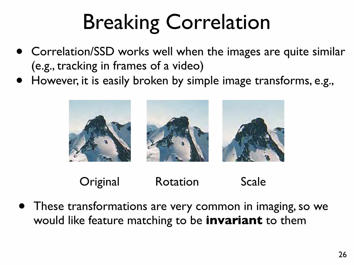
Breaking Correlation• Correlation/SSD works well when the images are quite similar

(e.g., tracking in frames of a video)

• However, it is easily broken by simple image transforms, e.g.,

26

Original Rotation Scale

• These transformations are very common in imaging, so wewould like feature matching to be invariant to them

Local Coordinate Frame• One way to achieve invariance is to use local coordinate

frames that follow the surface transformation

27

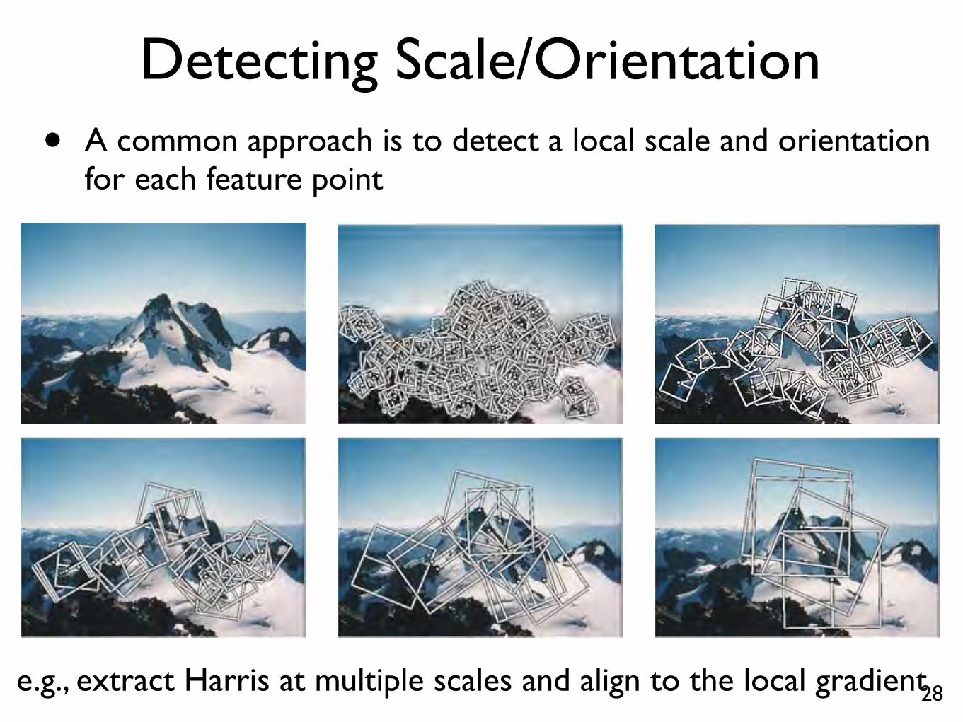
Detecting Scale/Orientation• A common approach is to detect a local scale and orientation

for each feature point

28


Figure 4.10 Multi-scale oriented patches (MOPS) extracted at five pyramid levels (Brown,Szeliski, and Winder 2005) c 2005 IEEE. The boxes show the feature orientation and theregion from which the descriptor vectors are sampled.

is unknown. Instead of extracting features at many different scales and then matching all ofthem, it is more efficient to extract features that are stable in both location and scale (Lowe2004; Mikolajczyk and Schmid 2004).

Early investigations into scale selection were performed by Lindeberg (1993; 1998b),who first proposed using extrema in the Laplacian of Gaussian (LoG) function as interestpoint locations. Based on this work, Lowe (2004) proposed computing a set of sub-octaveDifference of Gaussian filters (Figure 4.11a), looking for 3D (space+scale) maxima in the re-sulting structure (Figure 4.11b), and then computing a sub-pixel space+scale location using aquadratic fit (Brown and Lowe 2002). The number of sub-octave levels was determined, aftercareful empirical investigation, to be three, which corresponds to a quarter-octave pyramid,which is the same as used by Triggs (2004).

As with the Harris operator, pixels where there is strong asymmetry in the local curvatureof the indicator function (in this case, the DoG) are rejected. This is implemented by firstcomputing the local Hessian of the difference image D,

H =

"Dxx Dxy

Dxy Dyy

#, (4.12)

and then rejecting keypoints for which

Tr(H)2

Det(H)> 10. (4.13)

e.g., extract Harris at multiple scales and align to the local gradient

Detecting Scale/Orientation• Patch matching can be improved by using scale/orientation

and brightness normalisation

29

40 px

8 pixels

Sampling at a coarser scale than detection further improves robustness

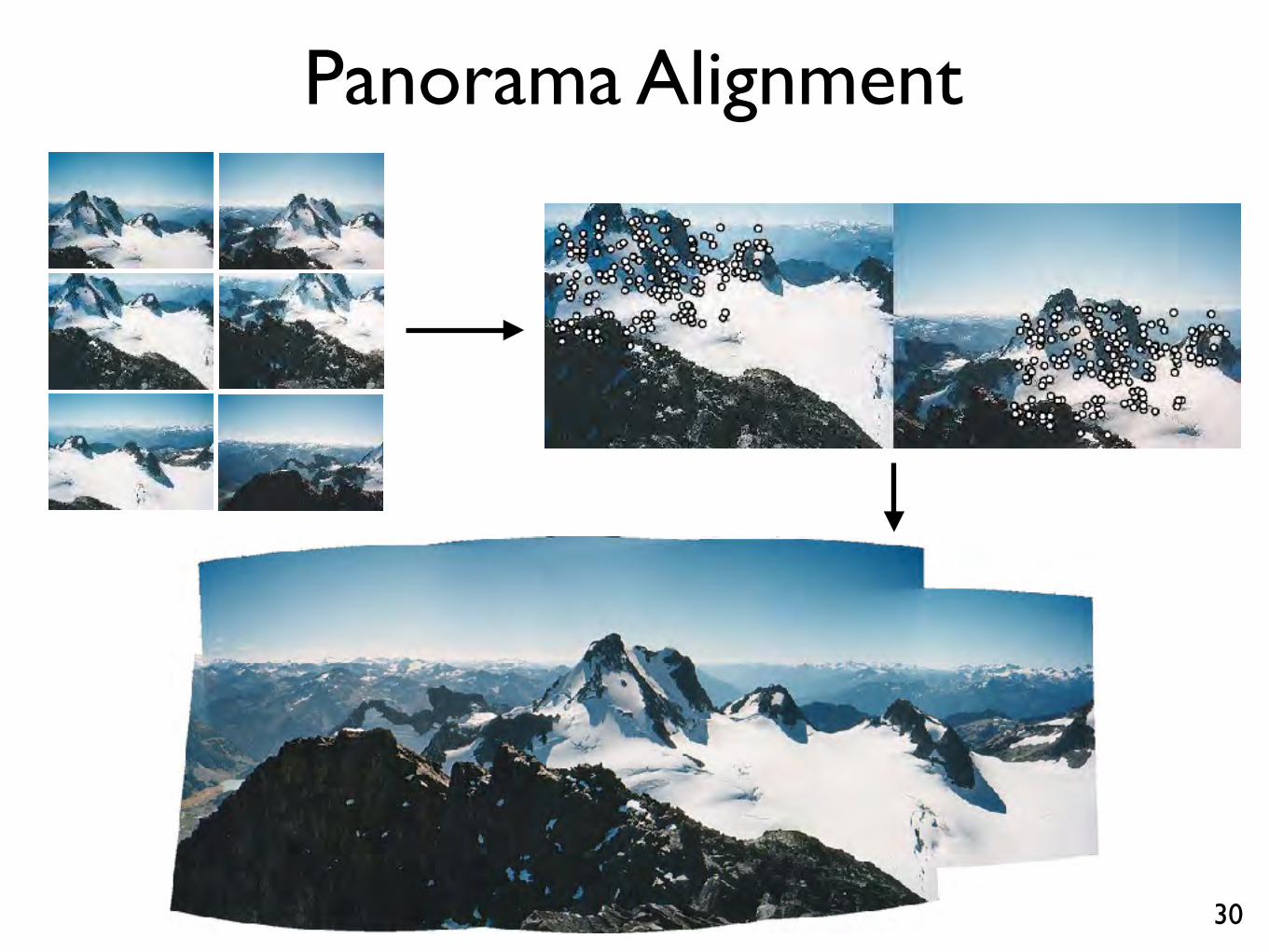
Panorama Alignment

30

Wide Baseline Matching• Patch-based matching works well for short baselines, but fails

for large changes in scale, rotation or 3D viewpoint

31What factors cause differences between these images?

Wide Baseline Matching• We would like to match patches despite these changes

32

What features of the local patch are invariant?

Scale Invariant Feature Transform• A detector and descriptor designed for object recognition

33

Figure 4: Top row shows model images for 3D objects withoutlines found by background segmentation. Bottom imageshows recognition results for 3D objectswithmodel outlinesand image keys used for matching.

mined by solving the corresponding normal equations,

which minimizes the sum of the squares of the distancesfrom the projected model locations to the corresponding im-age locations. This least-squares approach could readily beextended to solving for 3D pose and internal parameters ofarticulated and flexible objects [12].Outliers can now be removed by checking for agreement

between each image feature and themodel, given the param-eter solution. Each match must agree within 15 degrees ori-entation, change in scale, and 0.2 times maximummodelsize in terms of location. If fewer than 3 points remain afterdiscarding outliers, then thematch is rejected. If any outliersare discarded, the least-squares solution is re-solvedwith theremaining points.

Figure5: Examples of 3D object recognitionwith occlusion.

7. ExperimentsThe affine solution provides a good approximation to per-spective projection of planar objects, so planar models pro-vide a good initial test of the approach. The top row of Fig-ure 3 shows three model images of rectangular planar facesof objects. The figure also shows a cluttered image contain-ing the planar objects, and the same image is shown over-layed with the models following recognition. The modelkeys that are displayed are the ones used for recognition andfinal least-squares solution. Since only 3 keys are neededfor robust recognition, it can be seen that the solutions arehighly redundant and would survive substantial occlusion.Also shown are the rectangular borders of themodel images,projected using the affine transform from the least-squaresolution. These closely agree with the true borders of theplanar regions in the image, except for small errors intro-duced by the perspective projection. Similar experimentshave been performed formany images of planar objects, andthe recognition has proven to be robust to at least a 60 degreerotation of the object in any direction away from the camera.Although the model images and affine parameters do not

account for rotation in depth of 3D objects, they are stillsufficient to perform robust recognition of 3D objects overabout a 20 degree range of rotation in depth away from eachmodel view. An example of three model images is shown in

6








6








6








6








6








6

• SIFT features are invariant to translation, rotation and scale and slowly varying under perspective and 3D distortion

• Variants widely used in object recognition, image search etc.

[ Lowe 1999 ]

Scale Invariant Feature Transform

34

• Scale invariant detection and local orientation estimation

• Edge based representation that is robust to local shifting of edges (parallax and/or stretch)

[ vlfeat.org ]

http://vlfeat.org

SIFT Detection• Convolve with centre-surround Laplacian/DoG filter

35

=⇤

• Find all maxima at all scales in a Laplacian Pyramid

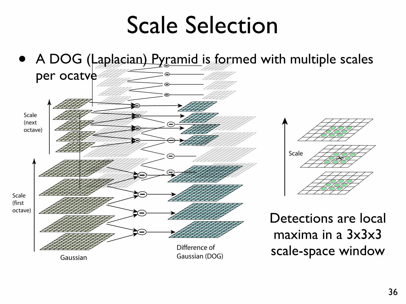
Scale Selection• A DOG (Laplacian) Pyramid is formed with multiple scales

per ocatve

36

Detections are localmaxima in a 3x3x3scale-space window


Scale (first octave)

Scale(nextoctave)

GaussianDifference ofGaussian (DOG)

. . .

Figure 1: For each octave of scale space, the initial image is repeatedly convolved with Gaussians toproduce the set of scale space images shown on the left. Adjacent Gaussian images are subtractedto produce the difference-of-Gaussian images on the right. After each octave, the Gaussian image isdown-sampled by a factor of 2, and the process repeated.

In addition, the difference-of-Gaussian function provides a close approximation to thescale-normalized Laplacian of Gaussian, �2r2G, as studied by Lindeberg (1994). Lindebergshowed that the normalization of the Laplacian with the factor �2 is required for true scaleinvariance. In detailed experimental comparisons, Mikolajczyk (2002) found that the maximaand minima of �2r2G produce the most stable image features compared to a range of otherpossible image functions, such as the gradient, Hessian, or Harris corner function.

The relationship betweenD and �2r2G can be understood from the heat diffusion equa-tion (parameterized in terms of � rather than the more usual t = �2):

@G

@�= �r2G.

From this, we see that r2G can be computed from the fi nite difference approximation to@G/@�, using the difference of nearby scales at k� and �:

�r2G =@G

@�⇡ G(x, y, k�) �G(x, y,�)

k� � �

and therefore,

G(x, y, k�) �G(x, y,�) ⇡ (k � 1)�2r2G.

This shows that when the difference-of-Gaussian function has scales differing by a con-stant factor it already incorporates the �2 scale normalization required for the scale-invariant

6

Scale

Figure 2: Maxima and minima of the difference-of-Gaussian images are detected by comparing apixel (marked with X) to its 26 neighbors in 3x3 regions at the current and adjacent scales (markedwith circles).

Laplacian. The factor (k � 1) in the equation is a constant over all scales and therefore doesnot influence extrema location. The approximation error will go to zero as k goes to 1, butin practice we have found that the approximation has almost no impact on the stability ofextrema detection or localization for even signifi cant differences in scale, such as k =

p2.

An effi cient approach to construction of D(x, y, ) is shown in Figure 1. The initialimage is incrementally convolved with Gaussians to produce images separated by a constantfactor k in scale space, shown stacked in the left column. We choose to divide each octaveof scale space (i.e., doubling of ) into an integer number, s, of intervals, so k = 21/s.We must produce s + 3 images in the stack of blurred images for each octave, so that fi nalextrema detection covers a complete octave. Adjacent image scales are subtracted to producethe difference-of-Gaussian images shown on the right. Once a complete octave has beenprocessed, we resample the Gaussian image that has twice the initial value of (it will be 2images from the top of the stack) by taking every second pixel in each row and column. Theaccuracy of sampling relative to is no different than for the start of the previous octave,while computation is greatly reduced.

3.1 Local extrema detection

In order to detect the local maxima and minima ofD(x, y, ), each sample point is comparedto its eight neighbors in the current image and nine neighbors in the scale above and below(see Figure 2). It is selected only if it is larger than all of these neighbors or smaller than allof them. The cost of this check is reasonably low due to the fact that most sample points willbe eliminated following the fi rst few checks.

An important issue is to determine the frequency of sampling in the image and scale do-mains that is needed to reliably detect the extrema. Unfortunately, it turns out that there isno minimum spacing of samples that will detect all extrema, as the extrema can be arbitrar-ily close together. This can be seen by considering a white circle on a black background,which will have a single scale space maximum where the circular positive central region ofthe difference-of-Gaussian function matches the size and location of the circle. For a veryelongated ellipse, there will be two maxima near each end of the ellipse. As the locations ofmaxima are a continuous function of the image, for some ellipse with intermediate elongationthere will be a transition from a single maximum to two, with the maxima arbitrarily close to

7

(a) (b)

Figure 4.11 Scale-space feature detection using a sub-octave Difference of Gaussian pyra-mid (Lowe 2004) c 2004 Springer: (a) Adjacent levels of a sub-octave Gaussian pyramidare subtracted to produce Difference of Gaussian images; (b) extrema (maxima and minima)in the resulting 3D volume are detected by comparing a pixel to its 26 neighbors.

While Lowe’s Scale Invariant Feature Transform (SIFT) performs well in practice, it is notbased on the same theoretical foundation of maximum spatial stability as the auto-correlation-based detectors. (In fact, its detection locations are often complementary to those producedby such techniques and can therefore be used in conjunction with these other approaches.)In order to add a scale selection mechanism to the Harris corner detector, Mikolajczyk andSchmid (2004) evaluate the Laplacian of Gaussian function at each detected Harris point (ina multi-scale pyramid) and keep only those points for which the Laplacian is extremal (largeror smaller than both its coarser and finer-level values). An optional iterative refinement forboth scale and position is also proposed and evaluated. Additional examples of scale invariantregion detectors are discussed by Mikolajczyk, Tuytelaars, Schmid et al. (2005); Tuytelaarsand Mikolajczyk (2007).

Rotational invariance and orientation estimation

In addition to dealing with scale changes, most image matching and object recognition algo-rithms need to deal with (at least) in-plane image rotation. One way to deal with this problemis to design descriptors that are rotationally invariant (Schmid and Mohr 1997), but suchdescriptors have poor discriminability, i.e. they map different looking patches to the samedescriptor.


Scale (first octave)

Scale(nextoctave)

GaussianDifference ofGaussian (DOG)

. . .

Figure 1: For each octave of scale space, the initial image is repeatedly convolved with Gaussians toproduce the set of scale space images shown on the left. Adjacent Gaussian images are subtractedto produce the difference-of-Gaussian images on the right. After each octave, the Gaussian image isdown-sampled by a factor of 2, and the process repeated.

In addition, the difference-of-Gaussian function provides a close approximation to thescale-normalized Laplacian of Gaussian, �2r2G, as studied by Lindeberg (1994). Lindebergshowed that the normalization of the Laplacian with the factor �2 is required for true scaleinvariance. In detailed experimental comparisons, Mikolajczyk (2002) found that the maximaand minima of �2r2G produce the most stable image features compared to a range of otherpossible image functions, such as the gradient, Hessian, or Harris corner function.

The relationship betweenD and �2r2G can be understood from the heat diffusion equa-tion (parameterized in terms of � rather than the more usual t = �2):

@G

@�= �r2G.

From this, we see that r2G can be computed from the fi nite difference approximation to@G/@�, using the difference of nearby scales at k� and �:

�r2G =@G

@�⇡ G(x, y, k�) �G(x, y,�)

k� � �

and therefore,

G(x, y, k�) �G(x, y,�) ⇡ (k � 1)�2r2G.

This shows that when the difference-of-Gaussian function has scales differing by a con-stant factor it already incorporates the �2 scale normalization required for the scale-invariant

6

Scale

Figure 2: Maxima and minima of the difference-of-Gaussian images are detected by comparing apixel (marked with X) to its 26 neighbors in 3x3 regions at the current and adjacent scales (markedwith circles).

Laplacian. The factor (k � 1) in the equation is a constant over all scales and therefore doesnot influence extrema location. The approximation error will go to zero as k goes to 1, butin practice we have found that the approximation has almost no impact on the stability ofextrema detection or localization for even signifi cant differences in scale, such as k =

p2.

An effi cient approach to construction of D(x, y, ) is shown in Figure 1. The initialimage is incrementally convolved with Gaussians to produce images separated by a constantfactor k in scale space, shown stacked in the left column. We choose to divide each octaveof scale space (i.e., doubling of ) into an integer number, s, of intervals, so k = 21/s.We must produce s + 3 images in the stack of blurred images for each octave, so that fi nalextrema detection covers a complete octave. Adjacent image scales are subtracted to producethe difference-of-Gaussian images shown on the right. Once a complete octave has beenprocessed, we resample the Gaussian image that has twice the initial value of (it will be 2images from the top of the stack) by taking every second pixel in each row and column. Theaccuracy of sampling relative to is no different than for the start of the previous octave,while computation is greatly reduced.

3.1 Local extrema detection

In order to detect the local maxima and minima ofD(x, y, ), each sample point is comparedto its eight neighbors in the current image and nine neighbors in the scale above and below(see Figure 2). It is selected only if it is larger than all of these neighbors or smaller than allof them. The cost of this check is reasonably low due to the fact that most sample points willbe eliminated following the fi rst few checks.

An important issue is to determine the frequency of sampling in the image and scale do-mains that is needed to reliably detect the extrema. Unfortunately, it turns out that there isno minimum spacing of samples that will detect all extrema, as the extrema can be arbitrar-ily close together. This can be seen by considering a white circle on a black background,which will have a single scale space maximum where the circular positive central region ofthe difference-of-Gaussian function matches the size and location of the circle. For a veryelongated ellipse, there will be two maxima near each end of the ellipse. As the locations ofmaxima are a continuous function of the image, for some ellipse with intermediate elongationthere will be a transition from a single maximum to two, with the maxima arbitrarily close to

7

(a) (b)

Figure 4.11 Scale-space feature detection using a sub-octave Difference of Gaussian pyra-mid (Lowe 2004) c 2004 Springer: (a) Adjacent levels of a sub-octave Gaussian pyramidare subtracted to produce Difference of Gaussian images; (b) extrema (maxima and minima)in the resulting 3D volume are detected by comparing a pixel to its 26 neighbors.

While Lowe’s Scale Invariant Feature Transform (SIFT) performs well in practice, it is notbased on the same theoretical foundation of maximum spatial stability as the auto-correlation-based detectors. (In fact, its detection locations are often complementary to those producedby such techniques and can therefore be used in conjunction with these other approaches.)In order to add a scale selection mechanism to the Harris corner detector, Mikolajczyk andSchmid (2004) evaluate the Laplacian of Gaussian function at each detected Harris point (ina multi-scale pyramid) and keep only those points for which the Laplacian is extremal (largeror smaller than both its coarser and finer-level values). An optional iterative refinement forboth scale and position is also proposed and evaluated. Additional examples of scale invariantregion detectors are discussed by Mikolajczyk, Tuytelaars, Schmid et al. (2005); Tuytelaarsand Mikolajczyk (2007).

Rotational invariance and orientation estimation

In addition to dealing with scale changes, most image matching and object recognition algo-rithms need to deal with (at least) in-plane image rotation. One way to deal with this problemis to design descriptors that are rotationally invariant (Schmid and Mohr 1997), but suchdescriptors have poor discriminability, i.e. they map different looking patches to the samedescriptor.

Scale Selection

36.1

12 Lindeberg

original image scale-space maxima of ( 2normL)2

(traceHnormL)2 (detHnormL)2

Figure 3: Normalized scale-space maxima computed from an image of a sunflower field: (topleft): Original image. (top right): Circles representing the 250 normalized scale-space maximaof (traceHnormL)2 having the strongest normalized response. (bottom left): Circles represent-ing scale-space maxima of (traceHnormL)2 superimposed onto a bright copy of the originalimage. (bottom right): Corresponding results for scale-space maxima of (detHnormL)2.


Figure 4: The 250 most significant normalized scale-space extrema detected from the per-spective projection of a sine wave of the form (with 10% added Gaussian noise).

[ T. Lindeberg ]

Scale Selection• Maximising the DOG function in scale as well as space

performs scale selection

37

12 Lindeberg

original image scale-space maxima of ( 2normL)2


Figure 3: Normalized scale-space maxima computed from an image of a sunflower field: (topleft): Original image. (top right): Circles representing the 250 normalized scale-space maximaof (traceHnormL)2 having the strongest normalized response. (bottom left): Circles represent-ing scale-space maxima of (traceHnormL)2 superimposed onto a bright copy of the originalimage. (bottom right): Corresponding results for scale-space maxima of (detHnormL)2.


Figure 4: The 250 most significant normalized scale-space extrema detected from the per-spective projection of a sine wave of the form (with 10% added Gaussian noise).

[ T. Lindeberg ]

Orientation Selection• To select a local orientation, build a histogram over orientation

38


Figure 4.12 A dominant orientation estimate can be computed by creating a histogram ofall the gradient orientations (weighted by their magnitudes or after thresholding out smallgradients) and then finding the significant peaks in this distribution (Lowe 2004) c 2004Springer.

A better method is to estimate a dominant orientation at each detected keypoint. Oncethe local orientation and scale of a keypoint have been estimated, a scaled and oriented patcharound the detected point can be extracted and used to form a feature descriptor (Figures 4.10and 4.17).

The simplest possible orientation estimate is the average gradient within a region aroundthe keypoint. If a Gaussian weighting function is used (Brown, Szeliski, and Winder 2005),this average gradient is equivalent to a first-order steerable filter (Section 3.2.3), i.e., it can becomputed using an image convolution with the horizontal and vertical derivatives of Gaus-sian filter (Freeman and Adelson 1991). In order to make this estimate more reliable, it isusually preferable to use a larger aggregation window (Gaussian kernel size) than detectionwindow (Brown, Szeliski, and Winder 2005). The orientations of the square boxes shown inFigure 4.10 were computed using this technique.

Sometimes, however, the averaged (signed) gradient in a region can be small and thereforean unreliable indicator of orientation. A more reliable technique is to look at the histogramof orientations computed around the keypoint. Lowe (2004) computes a 36-bin histogramof edge orientations weighted by both gradient magnitude and Gaussian distance to the cen-ter, finds all peaks within 80% of the global maximum, and then computes a more accurateorientation estimate using a three-bin parabolic fit (Figure 4.12).

Affine invariance

While scale and rotation invariance are highly desirable, for many applications such as widebaseline stereo matching (Pritchett and Zisserman 1998; Schaffalitzky and Zisserman 2002)or location recognition (Chum, Philbin, Sivic et al. 2007), full affine invariance is preferred.






Affine invariance


=

Selected orientation is peak in this histogram

SIFT Descriptor

39

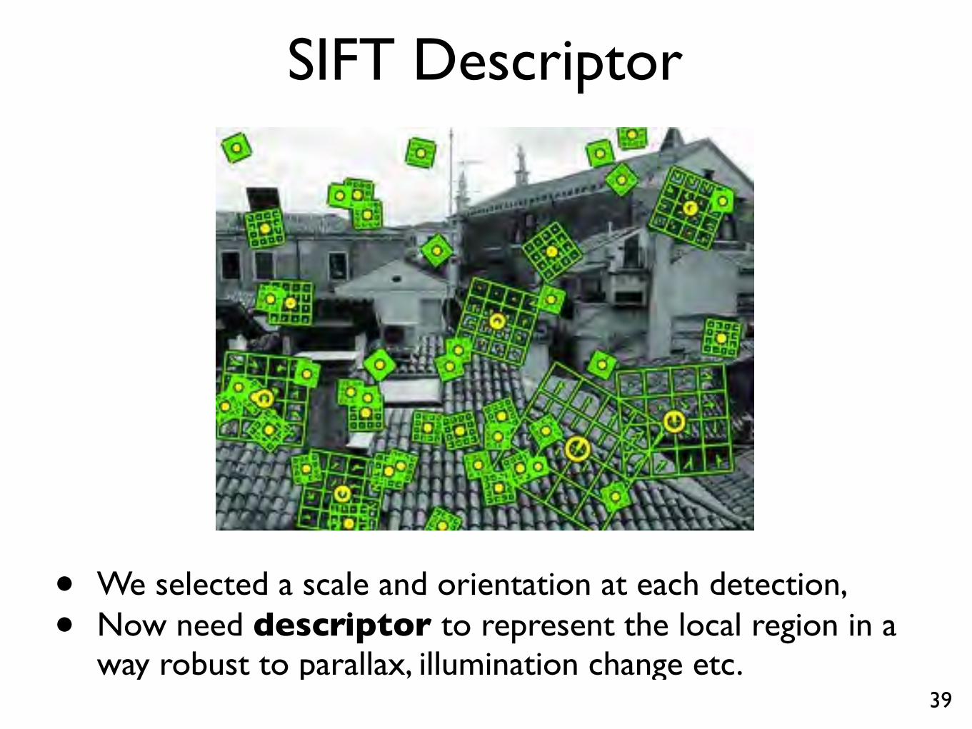
• We selected a scale and orientation at each detection,

• Now need descriptor to represent the local region in away robust to parallax, illumination change etc.

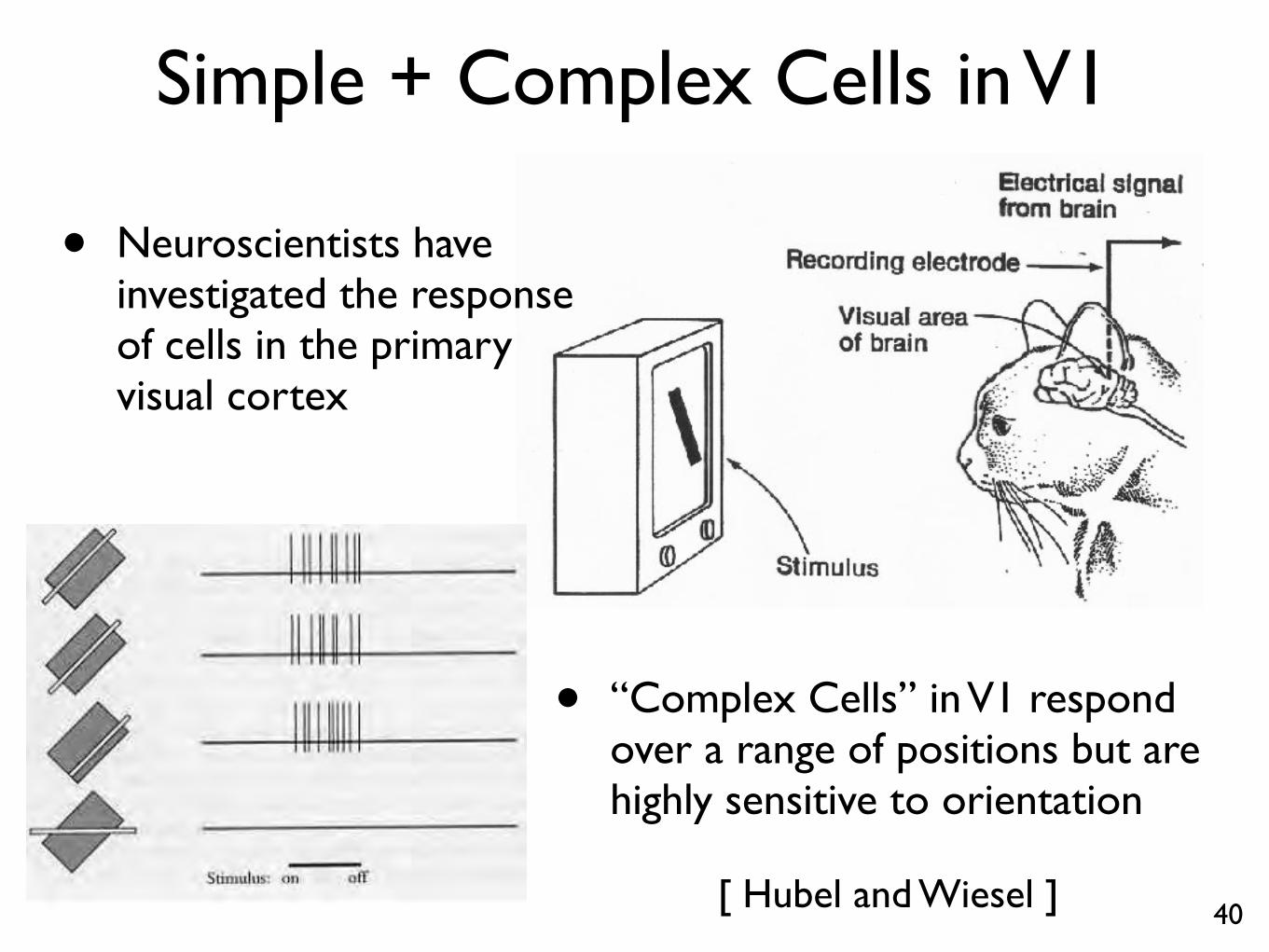
Simple + Complex Cells in V1

40[ Hubel and Wiesel ]

• Neuroscientists haveinvestigated the responseof cells in the primaryvisual cortex

• “Complex Cells” in V1 respondover a range of positions but arehighly sensitive to orientation

SIFT Descriptor• Describe local region by distribution (over angle) of gradients

41Each descriptor: 4 x 4 grid x 8 orientations = 128 dimensions

Image gradients Keypoint descriptor

Figure 7: A keypoint descriptor is created by first computing the gradient magnitude and orientationat each image sample point in a region around the keypoint location, as shown on the left. These areweighted by a Gaussian window, indicated by the overlaid circle. These samples are then accumulatedinto orientation histograms summarizing the contents over 4x4 subregions, as shown on the right, withthe length of each arrow corresponding to the sum of the gradientmagnitudes near that direction withinthe region. This figure shows a 2x2 descriptor array computed from an 8x8 set of samples, whereasthe experiments in this paper use 4x4 descriptors computed from a 16x16 sample array.

6.1 Descriptor representation

Figure 7 illustrates the computation of the keypoint descriptor. First the image gradient mag-nitudes and orientations are sampled around the keypoint location, using the scale of thekeypoint to select the level of Gaussian blur for the image. In order to achieve orientationinvariance, the coordinates of the descriptor and the gradient orientations are rotated relativeto the keypoint orientation. For efficiency, the gradients are precomputed for all levels of thepyramid as described in Section 5. These are illustrated with small arrows at each samplelocation on the left side of Figure 7.

A Gaussian weighting function with σ equal to one half the width of the descriptor win-dow is used to assign a weight to the magnitude of each sample point. This is illustratedwith a circular window on the left side of Figure 7, although, of course, the weight falls offsmoothly. The purpose of this Gaussian window is to avoid sudden changes in the descriptorwith small changes in the position of the window, and to give less emphasis to gradients thatare far from the center of the descriptor, as these are most affected by misregistration errors.

The keypoint descriptor is shown on the right side of Figure 7. It allows for significantshift in gradient positions by creating orientation histograms over 4x4 sample regions. Thefigure shows eight directions for each orientation histogram, with the length of each arrowcorresponding to the magnitude of that histogram entry. A gradient sample on the left canshift up to 4 sample positions while still contributing to the same histogram on the right,thereby achieving the objective of allowing for larger local positional shifts.

It is important to avoid all boundary affects in which the descriptor abruptly changes as asample shifts smoothly from being within one histogram to another or from one orientationto another. Therefore, trilinear interpolation is used to distribute the value of each gradientsample into adjacent histogram bins. In other words, each entry into a bin is multiplied by aweight of 1 − d for each dimension, where d is the distance of the sample from the centralvalue of the bin as measured in units of the histogram bin spacing.

15

Image gradients Keypoint descriptor

Figure 7: A keypoint descriptor is created by first computing the gradient magnitude and orientationat each image sample point in a region around the keypoint location, as shown on the left. These areweighted by a Gaussian window, indicated by the overlaid circle. These samples are then accumulatedinto orientation histograms summarizing the contents over 4x4 subregions, as shown on the right, withthe length of each arrow corresponding to the sum of the gradientmagnitudes near that direction withinthe region. This figure shows a 2x2 descriptor array computed from an 8x8 set of samples, whereasthe experiments in this paper use 4x4 descriptors computed from a 16x16 sample array.

6.1 Descriptor representation

Figure 7 illustrates the computation of the keypoint descriptor. First the image gradient mag-nitudes and orientations are sampled around the keypoint location, using the scale of thekeypoint to select the level of Gaussian blur for the image. In order to achieve orientationinvariance, the coordinates of the descriptor and the gradient orientations are rotated relativeto the keypoint orientation. For efficiency, the gradients are precomputed for all levels of thepyramid as described in Section 5. These are illustrated with small arrows at each samplelocation on the left side of Figure 7.

A Gaussian weighting function with σ equal to one half the width of the descriptor win-dow is used to assign a weight to the magnitude of each sample point. This is illustratedwith a circular window on the left side of Figure 7, although, of course, the weight falls offsmoothly. The purpose of this Gaussian window is to avoid sudden changes in the descriptorwith small changes in the position of the window, and to give less emphasis to gradients thatare far from the center of the descriptor, as these are most affected by misregistration errors.

The keypoint descriptor is shown on the right side of Figure 7. It allows for significantshift in gradient positions by creating orientation histograms over 4x4 sample regions. Thefigure shows eight directions for each orientation histogram, with the length of each arrowcorresponding to the magnitude of that histogram entry. A gradient sample on the left canshift up to 4 sample positions while still contributing to the same histogram on the right,thereby achieving the objective of allowing for larger local positional shifts.

It is important to avoid all boundary affects in which the descriptor abruptly changes as asample shifts smoothly from being within one histogram to another or from one orientationto another. Therefore, trilinear interpolation is used to distribute the value of each gradientsample into adjacent histogram bins. In other words, each entry into a bin is multiplied by aweight of 1 − d for each dimension, where d is the distance of the sample from the centralvalue of the bin as measured in units of the histogram bin spacing.

15






Affine invariance







Affine invariance


=

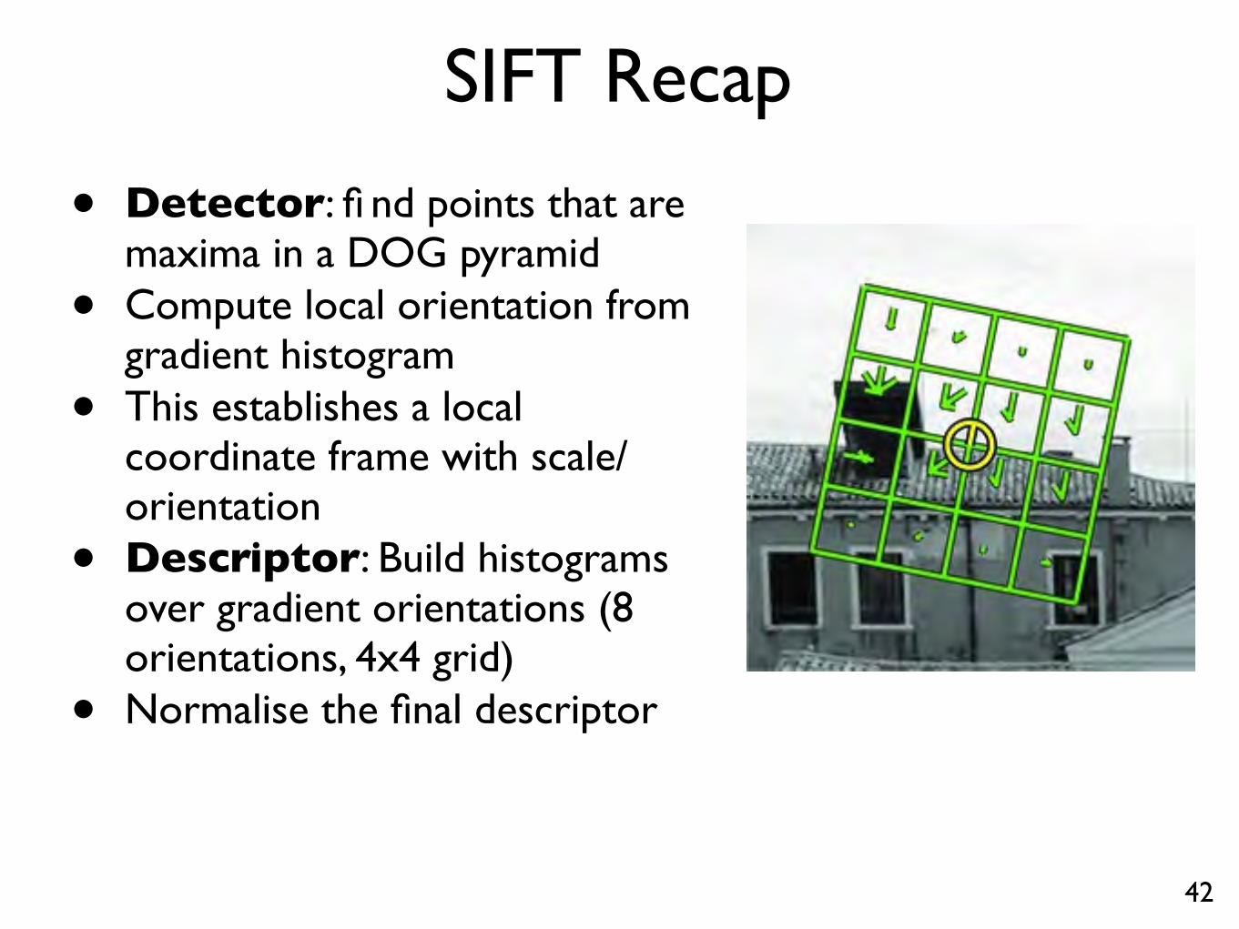
SIFT Recap

• Detector: fi nd points that aremaxima in a DOG pyramid

• Compute local orientation fromgradient histogram

• This establishes a localcoordinate frame with scale/orientation

• Descriptor: Build histogramsover gradient orientations (8 orientations, 4x4 grid)

• Normalise the final descriptor

42

SIFT Matching• Extract SIFT features from an image

43

Each image might generate 100’s or 1000’s of SIFT descriptors

SIFT Matching• Goal: Find all correspondences between a pair of images

44

?

• Extract and match all SIFT descriptors from both images

SIFT Matching• Each SIFT feature is represented by 128 numbers

• Feature matching becomes task of finding a nearby 128-dvector

• Nearest-neighbour matching:

45

NN(j) = argmini

|xi � xj |, i 6= j

• Linear time, but good approximation algorithms exist

• e.g., Best Bin First K-d Tree [Beis Lowe 1997], FLANN (FastLibrary for Approximate Nearest Neighbours) [Muja Lowe2009]

SIFT Matching• Feature matching returns a set of noisy correspondences

• To get further, we will have to know something about thegeometry of the images

46

Shape Context• Useful for matching with contours

47

A[ Belongie Malik 2000 ]

Descriptor is log polar histogram

Choosing Features• The best choice of features is usually application dependent

48

Shape context? SIFT? Something else?!"#$% !& '&%( #& # )'%*+ #,( -,% .-',/& /0% ,'"1%* -2.-**%./ !"#$%& !, /0% /-3 45 "#/.0%&6

7& /0!& %83%*!"%,/ !,9-:9%& !,/*!.#/% &0#3%& ;% !,<.*%#&%( /0% ,'"1%* -2 &#"3:%& 2*-" =55 /- >556 ?, &-"%.#/%$-*!%&@ /0% &0#3%& #33%#* *-/#/%( #,( 2:!33%(@ ;0!.0 ;%#((*%&& '&!,$ # "-(!2!%( (!&/#,.% 2',./!-,6 A0% (!&/#,.%(!&/!!"#" 1%/;%%, # *%2%*%,.% &0#3% ! #,( # )'%*+ &0#3%# !& (%2!,%( #&

!"#$!#"!" # %"&$!"#$!#"!$"" !"#$!#"!%"" !"#$!#"!&"%"

;0%*% !$"!%@ #,( !& (%,-/% /0*%% 9%*&!-,& -2 !B ',<.0#,$%(@ 9%*/!.#::+ 2:!33%(@ #,( 0-*!C-,/#::+ 2:!33%(6

D!/0 /0%&% .0#,$%& !, 3:#.% 1'/ -/0%*;!&% '&!,$ /0%&#"% #33*-#.0 #& !, /0% EF?GA (!$!/ %83%*!"%,/&@ ;%-1/#!, # *%/*!%9#: *#/% -2 HI6J= 3%*.%,/6 K'**%,/:+ /0% 1%&/3'1:!&0%( 3%*2-*"#,.% !& #.0!%9%( 1+ L#/%.M! %/ #:6 N>>O@;!/0 # *%/*!%9#: *#/% -2 HI64J 3%*.%,/@ 2-::-;%( 1+ E-M0/#*<!#, %/ #:6 #/ HJ644 3%*.%,/6

!"# $%&'()&%* +(,%-(.&/

A*#(%"#*M& #*% 9!&'#::+ -2/%, 1%&/ (%&.*!1%( 1+ /0%!* &0#3%!,2-*"#/!-,@ #,(@ !, "#,+ .#&%&@ &0#3% 3*-9!(%& /0% -,:+&-'*.% -2 !,2-*"#/!-,6 A0% #'/-"#/!. !(%,/!2!.#/!-, -2/*#(%"#*M !,2*!,$%"%,/ 0#& !,/%*%&/!,$ !,('&/*!#: #33:!.#</!-,&@ &!,.% ;!/0 /0% .'**%,/ &/#/% -2 /0% #*/ /*#(%"#*M& #*%1*-#(:+ .#/%$-*!C%( #..-*(!,$ /- /0% P!%,,# .-(%@ #,( /0%,"#,'#::+ .:#&&!2!%( #..-*(!,$ /- /0%!* 3%*.%3/'#: &!"!:#*!/+6Q9%, /0-'$0 &0#3% .-,/%8/ "#/.0!,$ (-%& ,-/ 3*-9!(% # 2'::&-:'/!-, /- /0% /*#(%"#*M &!"!:#*!/+ 3*-1:%" R-/0%* 3-/%,</!#: .'%& #*% /%8/ #,( /%8/'*%S@ !/ &/!:: &%*9%& ;%:: /- !::'&/*#/%/0% .#3#1!:!/+ -2 -'* #33*-#.0 /- .#3/'*% /0% %&&%,.% -2&0#3% &!"!:#*!/+6 ?, T!$6 =U@ ;% (%3!./ *%/*!%9#: *%&':/& 2-* #(#/#1#&% -2 >55 /*#(%"#*M&6 ?, /0!& %83%*!"%,/@ ;% *%:!%( -,#, #22!,% /*#,&2-*"#/!-, "-(%: #& $!9%, 1+ R>S@ #,( #& !, /0%3*%9!-'& .#&%@ ;% '&%( >55 &#"3:% 3-!,/&6

D% %83%*!"%,/%( ;!/0 %!$0/ (!22%*%,/ )'%*+ /*#(%"#*M&2-* %#.0 -2;0!.0 /0%(#/#1#&% .-,/#!,%( #/ :%#&/ -,%3-/%,/!#:!,2*!,$%"%,/6 D% (%3!./ /0% /-3 2-'* 0!/& #& ;%:: #& /0%!*&!"!:#*!/+ &.-*%6 ?/ !& .:%#*:+ &%%, /0#/ /0% 3-/%,/!#: !,2*!,$%<"%,/& #*% %#&!:+ (%/%./%( #,( #33%#* #& "-&/ &!"!:#* !, /0%/-3 *#,M& (%&3!/% &'1&/#,/!#: 9#*!#/!-, -2 /0% #./'#: &0#3%&6 ?/0#&1%%,"#,'#::+9%*!2!%( /0#/,-9!&'#::+ &!"!:#* /*#(%"#*M0#& 1%%, "!&&%( 1+ /0% #:$-*!/0"6

0 1231456723

D%0#9% 3*%&%,/%( # ,%;#33*-#.0 /- &0#3%"#/.0!,$67 M%+

.0#*#./%*!&/!. -2 -'* #33*-#.0 !& /0% %&/!"#/!-, -2 &0#3%

&!"!:#*!/+ #,( .-**%&3-,(%,.%& 1#&%( -, # ,-9%: (%&.*!3/-*@

/0% &0#3% .-,/%8/6 V'* #33*-#.0 !& &!"3:% #,( %#&+ /- #33:+@

+%/ 3*-9!(%& # *!.0 (%&.*!3/-* 2-* 3-!,/ &%/& /0#/ $*%#/:+

!"3*-9%& 3-!,/ &%/ *%$!&/*#/!-,@ &0#3% "#/.0!,$ #,( &0#3%

*%.-$,!/!-,6 ?, -'* %83%*!"%,/&@ ;% 0#9% (%"-,&/*#/%(

!"#$%&'" "( )#*+ ,-)." /)(0-'%& )%1 $!2"0( 3"0$&%'('$% 4,'%& ,-)." 0$%("5(, 678

9:;* 77* "<=>?@AB CD BE=?AB :F GEA /."&H I=G=J=BA DCK GEKAA I:DDAKAFG

L=GA;CK:AB*

9:;* 7M* (K=IA>=KN KAGK:AO=@ KABP@GB J=BAI CF = I=G=J=BA CD QRR I:DDAKAFGKA=@STCK@I GK=IA>=KNB* UA PBAI =F =DD:FA GK=FBDCK>=G:CF >CIA@ =FI =TA:;EGAI LC>J:F=G:CF CD BE=?A LCFGA<G B:>:@=K:GV '#' =FI GEA BP> COAK@CL=@ G=F;AFG CK:AFG=G:CF I:DDAKAFLAB*

Learning Descriptors• Descriptor design as a learning (embedding) problem

49[ Winder Brown 2007 ]

Learning Descriptors• Deep networks for descriptor learning

50

Preprocessing

Conv0

Pool0

Conv1

Pool1Metric network

Cross-Entropy Loss

Sampling

Conv2

Conv3

Conv4

Bottleneck

Pool4 FC2

FC1

FC3 + Softmax

A: Feature network B: Metric network

C: MatchNet in training

Figure 1. The MatchNet architecture. A: The feature network usedfor feature encoding, with an optional bottleneck layer to reducefeature dimension. B: The metric network used for feature com-parison. C: In training, the feature net is applied as two “towers”on pairs of patches with shared parameters. Output from the twotowers are concatenated as the metric network’s input. The entirenetwork is jointly trained on labeled patch-pairs generated fromthe sampler to minimize the cross-entropy loss. In prediction, thetwo sub-networks (A and B) are conveniently used in a two-stagepipeline (See Section 4.2).

[0, 1] from the two units of FC3, These are non-negative,sum up to one, and can be interpreted as the network’s es-timate of probability that the two patches match and do notmatch, respectively.

Two-tower structure with tied parameters: The patch-based matching task usually assumes that patches gothrough the same feature encoding before computing a sim-ilarity. Therefore we need just one feature network. Duringtraining, this can be realized by employing two feature net-works (or “towers”) that connect to a comparison network,with the constraint that the two towers share the same pa-rameters. Updates for either tower will be applied to theshared coefficients.

This approach is related to the Siamese network [2, 5],which also uses two towers, but with carefully designedloss functions instead of a learned metric network. A re-cent preprint on learning a network for stereo matching hasalso used the two-tower-plus-fully-connected comparison-network approach [37]. In contrast, MatchNet includesmax-pooling layers to deal with scale changes that are notpresent in stereo reconstruction problems, and it also has

Table 1. Layer parameters of MatchNet. The output dimensionis given by (height ⇥ width ⇥ depth). PS: patch size for con-volution and pooling layers; S: stride. Layer types: C: convo-lution, MP: max-pooling, FC: fully-connected. We always padthe convolution and pooling layers so the output height and widthare those of the input divided by the stride. For FC layers,their size B and F are chosen from: B 2 {64, 128, 256, 512},F 2 {128, 256, 512, 1024}. All convolution and FC layers useReLU activation except for FC3, whose output is normalized withSoftmax (Equation 2).

Name Type Output Dim. PS S

Conv0 C 64⇥ 64⇥ 24 7⇥ 7 1Pool0 MP 32⇥ 32⇥ 24 3⇥ 3 2Conv1 C 32⇥ 32⇥ 64 5⇥ 5 1Pool1 MP 16⇥ 16⇥ 64 3⇥ 3 2Conv2 C 16⇥ 16⇥ 96 3⇥ 3 1Conv3 C 16⇥ 16⇥ 96 3⇥ 3 1Conv4 C 16⇥ 16⇥ 64 3⇥ 3 1Pool4 MP 8⇥ 8⇥ 64 3⇥ 3 2Bottleneck FC B - -

FC1 FC F - -FC2 FC F - -FC3 FC 2 - -

more convolutional layers compared to [37].In other settings, where similarity is defined over patches

from two significantly different domains, the MatchNetframework can be generalized to have two towers that sharefewer layers or towers with different structures.

The bottleneck layer: The bottleneck layer can be usedto reduce the dimension of the feature representation and tocontrol overfitting of the network. It is a fully-connectedlayer of size B, between the 4096 (8 ⇥ 8 ⇥ 64) nodes inthe output of Pool4 and the final output of the feature net-work. We evaluate how B affects matching performance inSection 5 and plot results in Figure 4.

The preprocessing layer: Following a previous conven-tion, for each pixel in the input grayscale patch we normal-ize its intensity value x (in [0, 255]) to (x� 128)/160.

4. Training and predictionThe feature and metric networks are trained jointly in a

supervised setting using a two-tower structure illustrated inFigure 1-C. We minimize the cross-entropy error

E = � 1

n

nX

i=1

[yi log(yi) + (1� yi) log(1� yi)] (1)

over a training set of n patch pairs using stochastic gradientdescent (SGD) with a batch size of 32. Here yi is the 0/1label for input pair xi. 1 indicates match. yi and 1� yi arethe Softmax activations computed on the values of the two

[ MatchNetHan et al 2015 ]

Large-Scale Image Retrieval with Attentive Deep Local Features

Hyeonwoo Noh† Andre Araujo⇤ Jack Sim⇤ Tobias Weyand⇤ Bohyung Han†

†POSTECH, Korea{shgusdngogo,bhhan}@postech.ac.kr

⇤Google Inc.{andrearaujo,jacksim,weyand}@google.com

Abstract

We propose an attentive local feature descriptor suitable

for large-scale image retrieval, referred to as DELF (DEep

Local Feature). The new feature is based on convolutional

neural networks, which are trained only with image-level

annotations on a landmark image dataset. To identify

semantically useful local features for image retrieval, we

also propose an attention mechanism for keypoint selection,

which shares most network layers with the descriptor. This

framework can be used for image retrieval as a drop-in

replacement for other keypoint detectors and descriptors,

enabling more accurate feature matching and geometric

verification. Our system produces reliable confidence

scores to reject false positives—in particular, it is robust

against queries that have no correct match in the database.

To evaluate the proposed descriptor, we introduce a new

large-scale dataset, referred to as Google-Landmarks

dataset, which involves challenges in both database and

query such as background clutter, partial occlusion, multiple

landmarks, objects in variable scales, etc. We show that

DELF outperforms the state-of-the-art global and local

descriptors in the large-scale setting by significant margins.

Code and dataset can be found at the project webpage:

https://github.com/tensorflow/models/tree/master/research/delf.

1. Introduction

Large-scale image retrieval is a fundamental task in com-puter vision, since it is directly related to various practicalapplications, e.g., object detection, visual place recognition,and product recognition. The last decades have witnessedtremendous advances in image retrieval systems—from hand-crafted features and indexing algorithms [22, 33, 27, 16] to,more recently, methods based on convolutional neural net-works (CNNs) for global descriptor learning [2, 29, 11].

Despite the recent advances in CNN-based global descrip-tors for image retrieval in small or medium-size datasets [27,28], their performance may be hindered by a wide variety

'(/)�3LSHOLQH

/DUJH�6FDOH,QGH[

)HDWXUHV

'(/)�)HDWXUHV

4XHU\�,PDJH

'(/)�3LSHOLQH

,QGH[� 4XHU\�

11�)HDWXUHV

$WWHQWLRQ�6FRUHV

'DWDEDVH�,PDJHV

5HWULHYHG�,PDJHV

*HRPHWULF�9HULILFDWLRQ

Figure 1: Overall architecture of our image retrieval system, us-ing DEep Local Features (DELF) and attention-based keypointselection. On the left, we illustrate the pipeline for extraction andselection of DELF. The portion highlighted in yellow represents anattention mechanism that is trained to assign high scores to relevantfeatures and select the features with the highest scores. Featureextraction and selection can be performed with a single forwardpass using our model. On the right, we illustrate our large-scalefeature-based retrieval pipeline. DELF for database images areindexed offline. The index supports querying by retrieving nearestneighbor (NN) features, which can be used to rank database imagesbased on geometrically verified matches.

of challenging conditions observed in large-scale datasets,such as clutter, occlusion, and variations in viewpoint andillumination. Global descriptors lack the ability to find patch-level matches between images. As a result, it is difficult toretrieve images based on partial matching in the presence ofocclusion and background clutter. In a recent trend, CNN-based local features are proposed for patch-level matching[12, 42, 40]. However, these techniques are not optimizedspecifically for image retrieval since they lack the ability todetect semantically meaningful features, and show limitedaccuracy in practice.

Most existing image retrieval algorithms have been evalu-ated in small to medium-size datasets with few query images,i.e., only 55 in [27, 28] and 500 in [16], and the images inthe datasets have limited diversity in terms of landmark lo-cations and types. Therefore, we believe that the image

arX

iv:1

612.

0632

1v4

[cs.C

V]

3 Fe

b 20

18

[ DELFNoh et al 2017 ]

Patch labels Image labels, also learns interest function

Project 1

• You can now complete Project 1 — Descriptors andMatching and Testing and Improving FeatureMatching sections.

51

P1

Next Lecture

52

• Planar Geometry, Camera Models, RANSAC

features and matching - courses.cs.washington.edu

Documents