feasibilty study of upflow anaerobic filter for ... · thesis title: feasibility study of upflow...
TRANSCRIPT
FEASIBILTY STUDY OF UPFLOW ANAEROBIC FILTER FOR PRETREATMENT OF MUNICIPAL WASTEWATER
KRISHNAN KAVITHA (B.Eng, M.K UNIVERSITY,
M.Sc, NATIONAL UNIVERSITY OF SINGAPORE)
A THESIS SUMBITTED
FOR THE DEGREE OF MASTER OF ENGINEERING
DEPARTMENT OF CIVIL ENGINEERING
NATIONAL UNIVERSITY OF SINGAPORE
2009

i
Name: Krishnan Kavitha
Degree: M.Eng (Civil Engineering)
Dept: Civil Engineering
Thesis Title: Feasibility Study of Upflow Anaerobic Filter for Pretreatment of
Municipal Wastewater
SUMMARY
Anaerobic reactors have been successfully installed in full-scale plants world-wide
for treating high-strength industrial wastewater over the years. Recently, there has
been significant interest in exploring this technology for treating low-strength
domestic wastewater as well. Previously, it was thought that this was not practical as
methane fermentative process was considered too slow to be able to treat the
increasing volume of domestic sewage at a high rate. With technological advances
and better understanding of anaerobic microbial characteristics in recent years, there
is a potential that under control conditions, such barriers can be gradually overcome.
The perspectives of using anaerobic pre-treatment for domestic sewage are discussed
in this report to replace the conventional treatment methods. Feasibility of upflow
anaerobic filter (UAF) in place of activated sludge process to pre-treat domestic
wastewater is studied in this research.
Keywords: Anaerobic Filter, Sewage, COD, BOD, TSS and Methane.

ii
ACKNOWLEDGEMENTS
First and foremost to be acknowledged in this thesis is Dr.Ng How Yong,
who offered his generous support for me during project; his organization and professional
talents were indispensable. I am indebted to Prof. Ong Say Leong for his kind
encouragement to complete the project.
The assistance of a number of undergraduate and graduate students,
postdoctoral fellows, and colleagues was critical in this effort. I am very grateful to Mr.
Chandrasegaran, Lab Officer for his timely support. Special thanks and appreciation goes
to the postgraduate students Ms. Siow Woon, Mr. Sing Chuan and Ms. Wong Shih Wei
for their guidance to conduct the experiments. Successful completion of this project was
only possible through the professional and personal support of my friends and colleagues,
particularly in National University of Singapore. I am very grateful to Public Utilities
Board (PUB) Singapore for their financial support to this research.
I am also very grateful to the members of the Chemical and Environmental
Engineering Department of National University of Singapore for providing the numerous
facilities to accomplish the research successfully.
The last but not least, I am indebted to my husband, parents, sisters,
brothers and my son for their care, support and sacrifices to finish my research
successfully.
iii
TABLE OF CONTENTS SUMMARY i ACKNOWLEDGEMENT ii TABLE OF CONTENTS iii LIST OF FIGURES vi LIST OF TABLES viii NOMENCLATURE ix LIST OF APPENDIX-1 x 1. INTRODUCTION
1.1 Background 1 1.2 Objectives and Scope of the Study 4
2. LITERATURE REVIEW
2.1 Anaerobic treatment technology
2.1.1 Fundamentals of anaerobic decomposition 5 2.1.1.1 Anaerobic bacteria 5 2.1.1.2 Pathways in anaerobic degradation of organic waste 5
2.1.2 Kinetics of anaerobic decomposition 11 2.1.3 Factors anaerobic treatment 14 2.1.4 Advantages of anaerobic treatment systems 17 2.2 Positive perspectives for applicability of anaerobic sewage treatment plant 18 2.2.1 Temperature in tropical countries 18 2.2.2 Wastewater organic strength 20 2.2.3 Total Kjeldahl Nitrogen (TKN) and Ammonical Nitrogen (NH4
+-N) 21 2.2.4 Fatty Acids 22 2.2.5 pH 22 2.2.6 Sulfate 22 2.2.7 Toxicants 23

iv
2.2.8 Flow rate of the wastewater 23
2.3 Application of anaerobic treatment technology for municipal wastewater 24 2.3.1 Perspectives of anaerobic-aerobic systems 24 2.3.2 Necessity of aerobic post-treatment systems 24 2.3.3 Assessment of technological requirements for combined systems 26 2.4 Progress of anaerobic digestion technology for municipal wastewater 26
2.5 Upflow anaerobic filter (UAF) 29 2.5.1 Origin and Development of Anaerobic Filter 32
3. MATERIALS AND METHODS 3.1 Lab Scale Upflow Anaerobic Filter 3.1.1 Experimental Set-up of Anaerobic Filters 43 3.1.2 Biomass Seeding 46 3.1.3 Operational Conditions 46 3.2 Analytical Methods 3.2.1 Solids Concentration 48 3.2.2 Chemical Oxygen Demand 48 3.2.3 Biological Oxygen Demand 48
3.2.4 Biogas Composition 49 3.2.5 Total Nitrogen 49
3.2.6 Total Phosphate 49 3.2.7 Volatile Fatty Acids 50 3.2.8 Ammonical Nitrogen 51 3.2.9 Total Organic Carbon (TOC) 51 3.2.10 Anion 51 3.2.11 Hydrogen Sulphide 52 3.2.12 Alkalinity 52 3.2.13 Molecular Weight Distribution 52 3.2.14 EPS Extraction 53
v
4. RESULTS AND DISCUSSION 4.1 Suspended Solids Removal 57 4.2 Volatile suspended solids removal 65
4.3 Chemical Oxygen Demand Removal 70
4.4 Biochemical Oxygen Demand Removal 79 4.5 Biogas Composition 87 4.6 Biogas Production 90 4.7 Suspended biomass 93 4.8 Attached biomass 96 4.9 Mass balance 97 4.10 Operational Problems 99 5. CONCLUSION AND RECOMMEDATIONS 5.1 Conclusion 100 5.2 Recommendations 101 6. REFERENCES 103 7. APPENDIX Appendix-1 114

vi
LIST OF FIGURES
Figure 2.1 Pathways in anaerobic degradation 6
Figure 2.2 Growth rates of methanogens 15
Figure 2.3 Simplified comparison of aerobic vs anaerobic processes 17
Figure 2.4 World temperature zones 19
Figure 2.5 Principal differences between anaerobic and aerobic intensive wastewater treatment 25 Figure 2.6 Schematic diagram of an upflow anaerobic filter 31
Figure 3.1 Picture of upflow anaerobic filters 44
Figure 3.2 Schematic diagram of UAF experimental set-up 45
Figure 4.1 Influent and effluent SS & VSS concentrations and removal efficiencies of UAF1 at HRT 16, 8 & 4hrs 61
Figure 4.2 Influent and effluent SS & VSS concentrations and removal efficiencies of UAF2 at HRT 12 & 6 hrs 62
Figure 4.3 Influent and effluent suspended solids concentrations and removal efficiencies of UAF2 at HRT of 6 and 4 hours 64
Figure 4.4 Influent and effluent volatile suspended solids concentrations and removal efficiencies of UAF2 at HRT of 6 and 4 hours 69
Figure 4.5 Influent and effluent tCOD & sCOD concentrations and removal efficiencies of UAF1 at HRT 16, 8 and 4 hours 73
Figure 4.6 Influent and effluent tCOD & sCOD concentrations and removal efficiencies of UAF2 at HRT 12 and 6 hours 74
Figure 4.7 Influent and effluent tCOD concentrations and removal efficiencies of UAF2 at fluctuating HRTs 77
vii
Figure 4.8 Influent and effluent sCOD concentrations and removal efficiencies of UAF2 at fluctuating HRTs 78
Figure 4.9 Influent and effluent tBOD & sBOD concentrations and removal efficiencies of UAF1 at HRT 16, 8 and 4 hours 80
Figure 4.10 Influent and effluent tBOD & sBOD concentrations and removal efficiencies of UAF2 at HRT 12 and 6 hours 81
Figure 4.11Influent and effluent tBOD concentrations and removal efficiencies of UAF2 at fluctuating HRTs 84
Figure 4.12 Influent and effluent sBOD concentrations and removal efficiencies of UAF2 at fluctuating HRTs 84 Figure 4.13 Biogas composition of UAF2 88 Figure 4.14 Biogas composition of UAF1 89 Figure 4.15 Biogas production of UAF1 91 Figure 4.16 Biogas production of UAF2 92 Figure 4.17 MLSS & MLVSS concentrations in UAF2 94 Figure 4.18 MLSS & MLVSS concentrations in UAF1 95

viii
LIST OF TABLES Table 2.1 List of hydrolytic bacteria and extracellular enzymes 7 Table 2.2 List of acidogens involved in acidogenesis 8
Table 2.3 List of acitogens involved in acitogenesis 9 Table 2.4 List of methanogens involved in methanogenesis 10 Table 2.5 Important kinetic constants for acid and methanogenic fermentation 14
Table 2.6 Composition ranges of municipal wastewater for industrialized Countries 21 Table 2.7 Comparison of different anaerobic process behavior 28 Table 2.8 List of review plants in various studies 36 Table 2.9 Quality requirements of packing media for an anaerobic filter 42 Table 4.1 Influent and effluent suspended solids concentrations and
removal efficiencies 59 Table 4.2 Influent and effluent suspended solids concentrations and
removal efficiencies of UAF2 at fluctuating loading rates 63 Table 4.3 Influent and effluent volatile suspended solids concentrations and removal efficiencies 66 Table 4.4 Influent and effluent volatile suspended solids concentrations and removal efficiencies of UAF2 at fluctuating HRTs 67 Table 4.5 Influent and effluent tCOD & sCOD concentrations and removal efficiencies 72 Table 4.6 Influent and effluent tCOD & sCOD concentrations and removal efficiencies of UAF2 at fluctuating HRTs 76 Table 4.7 Influent and effluent tBOD & sBOD concentrations and removal efficiencies 82 Table 4.8 Influent and effluent tBOD & sBOD concentrations and removal efficiencies of UAF2 at fluctuating HRTs 85

ix
NOMENCLATURE
Symbol Referent
ASP Activated sludge process
BOD Biochemical Oxygen Demand
COD Chemical Oxygen Demand
HRT Hydraulic Retention Time
sBOD Soluble BOD
sCOD Soluble COD
SS Suspended Solids
tBOD Total BOD
tCOD Total COD
VFA Volatile Fatty Acids
VSS Volatile Suspended Solids
WRP Water Reclamation Plant

x
LIST OF APPENDIX-1
Protocol 1 EPS Extraction 114 Protocol 4 SS and VSS measuring procedure 115

1
CHAPTER 1 INTRODUCTION
1.1 Background
With increasing world population and demand for more fresh water, recycling and
reuse of wastewater has gained popularity among countries and industries in recent
years. Water reclamation on treated effluent has now been considered as one of the
alternative sources for water, especially for regions that face water scarcity issues.
Therefore, reclamation of wastewater has the double advantage of reducing the demand
for fresh water and protecting the water quality of the receiving bodies.
About one-third of the world's population lives in countries with moderate to high
water stress, and problems of water scarcity are increasing, partly due to ecosystem
depletion and contamination. Two out of every three persons on the globe may be
living in water-stressed conditions by the year 2025, if present global consumption
patterns continue (WHO, 2000). Meanwhile, water consumption has increased nine fold
and industrial water consumption has risen by a factor of 40. Yet water as a resource is
limited and poorly distributed. "The quantity of available water remains the same. Its
scarcity could be a serious obstacle to development in the millennium” (GEO, 1999).
For decades, Singapore has relied on import from Malaysia to supply half of the
water consumption in Singapore. However the two water agreements that supply
Singapore this water are due to expire by 2011 and 2061, respectively, and the two
countries are engaged in an on-going discussion over the price of raw water. Without a
workable resolution, the government of Singapore decided to increase self-sufficiency

2
in its water supply. Once wastewaters are produced and collected in sewerage systems,
treatment becomes a necessity. Yet, wastewater management is a costly business.
Water reclamation plants in Singapore treated about 511 million cubic meters of used
water in the year 2006 (PUB, 2006). The Keppel Seghers Ulu Pandan NEWater Plant
has a capacity to produce 32 mgd (148,000 m3/day) of NEWater to supply over 50
percent of Singapore’s current NEWater needs. Therefore, water reuse can be a better
option to solve water requirement in tropical countries like Singapore to some extent.
The current wastewater treatment in Singapore follows mainly the conventional
treatment train. Most conventional wastewater treatment processes are aerobic; that is,
the bacteria used to break down the waste products take in oxygen to perform their
function. This results in high energy consumption, huge land area requirement and a
large volume of waste sludge being produced. Indeed, treatment and disposal of sewage
sludge is technically cumbersome and economically a heavy burden. This makes the
processes complicated to control and costly to operate. To overcome these problems,
anaerobic treatment system can be an alternative to treat domestic wastewater in
Singapore, where land and sludge disposal is a major concern.
The bacteria in anaerobic processes do not use oxygen. Therefore, the energy
requirement and sludge production are much lesser than aerobic processes, making
anaerobic processes becoming cheaper alternative. Ng and Chin (1987) reported that
anaerobic digestion processes are energy efficient as they do not need to transfer large
quantities of oxygen into the wastewater. Sludge management requirements are also

3
reduced because the process produces substantially less biological solids than
conventional aerobic treatment processes. In addition, the methane-rich biogas
generated by the process is a convenient energy source for plant operation.
It is often questioned why aerobic treatment of municipal wastewater is not
replaced more rapidly by the economically more attractive and the conceptually more
holistic anaerobic treatment. Also, the temperature range conducive for bacteria is very
much suited for hot climates like in Singapore.
Anaerobic reactors have been successfully installed in full-scale plants world-
wide for treating high-strength industrial wastewater over the years. Recently, there has
been significant interest in exploring this technology for treating low-strength domestic
wastewater as well. Previously, it was thought that anaerobic process was not practical
as methane fermentative process was considered too slow for treating the increasing
volume of domestic sewage at a high rate. With technological advances and better
understanding of anaerobic microbial characteristics in recent years, there is a potential
that under control conditions, such barriers can be gradually overcome. The
perspectives of using anaerobic pre-treatment for domestic sewage are discussed in this
report to replace the conventional treatment methods.
4
1.2 Objectives and Scope of the Study
The scopes of this study covered:
1. Feasibility study on using selected anaerobic treatment technology in place of
activated sludge process to pre-treat domestic wastewater using bench-scale
systems.
2. Performance examination of an upflow anaerobic filter (UAF) at hydraulic
retention times of 16, 12, 8, 6 and 4hrs.
3. Optimize the anaerobic processes for maximal energy production and organic
removal.
The specific objectives of the study were: (1) to determine the stability of the
process at short HRTs, (2) to examine its treatment efficiencies, and (3) to
compare process parameters and performances with other studies.

1
CHAPTER 2 LITERATURE REVIEW
2.1 Anaerobic Treatment Technology
2.1.1 Fundamentals of Anaerobic Decomposition
2.1.1.1 Anaerobic Bacteria
Anaerobes (literally meaning "without air") are organisms that do not use oxygen
to live. Anaerobic organisms use different molecules as electron acceptors, such as
sulfide or carbon dioxide. In fact, these organisms are incredibly diverse when it comes to
the nutrients that they can use to survive.
2.1.1.2 Pathways in Anaerobic Degradation of Organic Waste
The use of anaerobes in the absence of oxygen for the stabilization of organic
material by conversion to methane, carbon dioxide, new biomass and inorganic products
is know as anaerobic degradation. There are three distinct phases, namely, hydrolysis,
acidogenesis and methanogenesis. The diagram of the process of anaerobic degradation is
presented in Figure 2.1.
The anaerobic process is different from the aerobic process in a way that it occurs
in the absence or very low amounts of oxygen such that aerobic reactions, in which
oxygen act as the electron acceptors, cannot take place. This process involves 4 main
phases where different types of bacteria, which will be mentioned below, convert large
complex organics into smaller compounds such as methane. These bacteria depend on
each other to achieve a balanced growth. The breakdown of organics under anaerobic
condition is given in Equation 2.1.

2
Anaerobic overall equation:
Organics � CH4 + CO2 + H2 + NH3 + H2S (2.1)
Figure 2.1 Pathways in Anaerobic Degradation
Hydrolysis
Hydrolysis is the first step in the anaerobic process, in which particulate matter is
converted to soluble compounds that can be hydrolyzed further to simple monomers that
are used by bacteria that perform fermentation. This step is necessary to allow the organic
materials to pass through the bacterial cell walls for use as energy to meet metabolic
requirements. This is done by the excrement of extra-cellular and hydrolytic enzymes. In
the anaerobic processes, hydrolysis would be best described as a first order process with
respect to the concentration of degradable particulate organic matter. Table 2.1 shows the
list of hydrolytic bacteria and extra-cellular enzymes that involved in hydrolysis process
Carbohydrates
Fats
Proteins
Acetic Acid CO2 H2 CO2
H2 NH3 Amnio
Acids
Fatty Acids
Sugars
Carbon Acids Alcohols
CH4 CO2
Hydrolysis Methanogenesis Acetogenesis Acedogenesis

3
to degrade complex organic compounds such as protein, carbohydrate and lipid (Maier et
al., 2000).
Factors which affect the rate of hydrolysis include pH, sludge retention time (SRT) and
particulate size of substrate. In hydrolysis, there is no reduction of chemical oxygen
demand (COD) as macromolecules are merely broken down into monomers. Soluble
COD is expected to increase due to the hydrolysis of macromolecules into soluble
organic products.
Table 2.1 List of hydrolytic bacteria and extracellular enzymes (Maier et al., 2000)
Complex Organic Compound Hydrolytic Bacteria Extracellular Enzyme
Protein Clostridium, Bacillus, Vibrio Peptococcus
Protese
Carbohydrate Clostridium, Acetovibrio celluliticus, Bactriodes
Cellulase, Amylase, Xylanase
Lipid Clostridium, Micrococcus Lipase, Phospolipase
Acidogenesis
Acidogenesis is the second step in the anaerobic process. The complex organic matter
that has been hydrolyzed ferment to long chain organic acids, sugars and amino acids,
after which, they are degraded further. Organic substances serve the function of both
electron acceptors and donators. The principal products are acetate, hydrogen, carbon
dioxide, propionate and butyrate. This stage of the anaerobic degradation is mediated by
facultative and obligate bacteria. Studies have shown that the obligate anaerobes form the

4
larger portion of the acidogenic bacteria as compared to the facultative anaerobes (Maier
et al., 2000).
In this step, COD reduction is due to the conversion of soluble organics to biomass and to
biogas in the form of carbon-di-oxide (CO2) and hydrogen (H2). Most of the COD is still
in the soluble state; however, it has been changed to acetate and other volatile fatty acids
(VFAs). Table 2.2 shows the list of acidogenic bacteria involved during acidogenesis
process (Maier et al., 2000).
Table 2.2 List of acidogens involved in acidogenesis (Maier et al., 2000)
Source Product Acidogen Product
Long chain fatty acids, glycerol
Clostridium Higher VFAs, Acetate, H2, CO2
Sugar, amino acids Clostridium, Strptococcus, Eubactrium limosum Zymomonas mobilis Lactobacillus, Micrococcus, Escherichia, Pseudomonas, Staphylococcus, Bacillus, Desulfovibrio, Selenomonas, Veillonella, Sarcina, Streptococcus, Desulfobacter, Desulfuromonas
Higher VFAs Long chain fatty acids, alcohol Acetate, H2, CO2
5
Acetogenesis
This stage is a subset of acidogenesis and involves the oxidation of long chain fatty acids,
propionate and butyrate by obligate anaerobes to produce hydrogen, carbon dioxide and
acetate. Even number carbon atom acids are degraded to acetate, whereas odd number
carbon acids are degraded to acetate and hydrogen ion (H+).
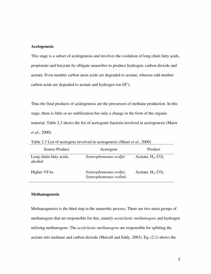
Thus the final products of acidogenesis are the precursors of methane production. In this
stage, there is little or no stabilization but only a change in the form of the organic
material. Table 2.3 shows the list of acetogenic bacteria involved in acetogenesis (Maier
et al., 2000).
Table 2.3 List of acetogens involved in acetogenesis (Maier et al., 2000)
Source Product Acetogens Product
Long chain fatty acids, alcohol
Syntrophomonas wolfei Acetate, H2, CO2
Higher VFAs Syntrophomonas wolfei, Syntrophomonas wolinii
Acetate, H2, CO2
Methanogenesis
Methanogenesis is the third step in the anaerobic process. There are two main groups of
methanogens that are responsible for this, namely aceticlastic methanogens and hydrogen
utilizing methanogens. The aceticlastic methanogens are responsible for splitting the
acetate into methane and carbon dioxide (Metcalf and Eddy, 2003). Eq. (2.1) shows the

6
splitting of acetate into methane and carbon dioxide while Eq. (2.1) shows the reduction
of carbon dioxide in the presence of hydrogen.
Acetotrophic:
CH3COOH � CH4 + CO2 ∆ Go = -32 kJ (2.2)
Hydrogenotrophic:
CO2 + 4H2 � CH4 + 2H2O ∆ Go = -138.9 kJ (2.3)
The second group use hydrogen as the electron donor and carbon dioxide as the electron
acceptor to produce methane. These are the acetogens which are also able to use carbon
dioxide to oxidize hydrogen and form acetic acid. Methane fermentation is very
important in the anaerobic treatment process. Stabilization of the organic material occurs
when acetic acid is converted to methane. In general, about 72% of methane produced in
an anaerobic process is from acetate formation (Metcalf and Eddy, 2003). The other 28%
is contributed by the reduction of carbon dioxide using hydrogen as the energy source by
carbon dioxide reducing bacteria (Henze et al., 1983; Parkin et al., 1986). It is also noted
that high concentrations of propionate or butyrate is indicative of reactor failure, and
propionate, in particular, is toxic to the acetogens (Parkin and Owen, 1986). Table 2.4
shows the list of methanogens involved in methanogenesis (Maier et al., 2000).
Table 2.4 List of methanogens involved in methanogenesis (Maier et al., 2000)
Source Product Methanogen Product
Acetate Methanotrix, Methanosarcina, Methanospirillum
CH4, CO2
7
H2, CO2 Methanobactrium, Methanoplanus, Methanobrevibacterium
CH4
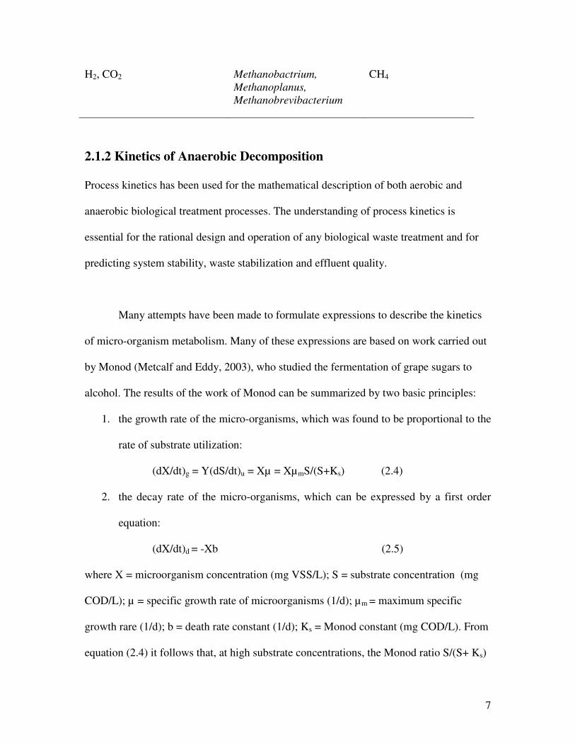
2.1.2 Kinetics of Anaerobic Decomposition
Process kinetics has been used for the mathematical description of both aerobic and
anaerobic biological treatment processes. The understanding of process kinetics is
essential for the rational design and operation of any biological waste treatment and for
predicting system stability, waste stabilization and effluent quality.
Many attempts have been made to formulate expressions to describe the kinetics
of micro-organism metabolism. Many of these expressions are based on work carried out
by Monod (Metcalf and Eddy, 2003), who studied the fermentation of grape sugars to
alcohol. The results of the work of Monod can be summarized by two basic principles:
1. the growth rate of the micro-organisms, which was found to be proportional to the
rate of substrate utilization:
(dX/dt)g = Y(dS/dt)u = Xµ = XµmS/(S+Ks) (2.4)
2. the decay rate of the micro-organisms, which can be expressed by a first order
equation:
(dX/dt)d = -Xb (2.5)
where X = microorganism concentration (mg VSS/L); S = substrate concentration (mg
COD/L); µ = specific growth rate of microorganisms (1/d); µm = maximum specific
growth rare (1/d); b = death rate constant (1/d); Ks = Monod constant (mg COD/L). From
equation (2.4) it follows that, at high substrate concentrations, the Monod ratio S/(S+ Ks)
8
approaches unity and the growth rate becomes independent of the substrate concentration,
i.e. it becomes a zero-order process. If the substrate concentration is low (S<< Ks), the
Monod ratio approaches S/Ks and the growth rate is proportional to the substrate
concentration, which is characteristic of a first-order process. For intermediate
concentrations the growth rate is between zero and first order with respect to the substrate
concentration.
The specific growth rates of Methanotrix and Methanosarcina are 0.1 and 0.3 d-1,
respectively (Adrianus and Lettinga, 1994). The specific growth rate is at half its
maximum value when the substrate concentration is equal to the parameter Ks, which, for
that reason, is called the half-saturation constant or affinity constant. For Methanotrix and
Methanosarcina the values of Ks are 200 and 30 mg/L acetate, respectively. At low
acetate concentration (<55 mg/L) the specific growth rate of Methanotrix becomes higher
than that of Methanosarcina. By contrast, at acetate concentrations exceeding 55 mg/L,
Methanosarcina will out-compete Methanotrix and become the prevailing acetate-
consuming organism.
In sewage treatment practice the substrate concentration will not be the minimum
obtainable, because this would require a very long retention time and hence an
unacceptably large treatment process. If the substrate concentration is greater than the
minimum there will be a net growth of microorganisms. Naturally, the increase in the
microorganism mass cannot go on indefinitely: after some time of operation the system
will be full and wastage of microorganism mass becomes unavoidable. If it is assume that
9
the microorganisms produced in a completely mixed treatment system are wasted at a
constant rate, this rate will be equal to the net production rate. In that case a constant
microorganism mass and concentration, compatible with the organic load entering the
system, will establish itself. The rate of wastage is the inverse of the sludge age, which
denotes the average solids retention time. Thus for a steady-state system
(dX/dt)w = (dX/dt)g + (dX/dt)d (2.6)
Or X/Rs = X(µ-b) (2.7)
where X = microorganism concentration (mg VSS/L)
(dX/dt)w = rate of wastage
(dX/dt)g = growth rate of the micro-organisms
dX/dt)d = decay rate of the micro-organisms
Rs = Sludge age
The following expression is for the effluent substrate concentration:
S = Ks(b+1)/Rs)/[�m-(b+1/Rs)] (2.8)
Equation (2.8) shows that the effluent concentration depends upon the values of three
constants (Ks, �m and b) and one process variable: sludge age, Rs.
Another important kinetic parameter is the maximum specific substrate utilization rate,
Km. This constant denotes the maximum mass of substrate that can be metabolized per
unit time. Specific substrate utilization rate can be calculated from the maximum specific
growth rate and the yield coefficient as follows:
Km = �m /Y (2.9) Km = specific substrate utilization rate (kg COD/kg VSS/d)
10
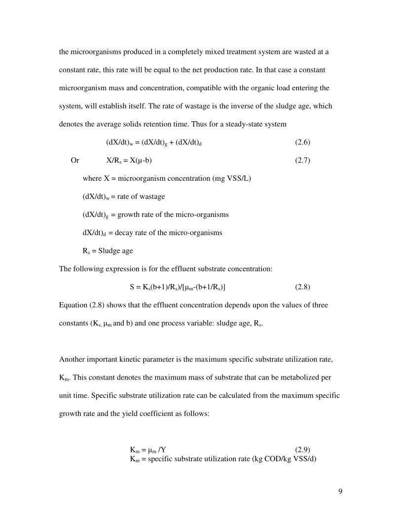
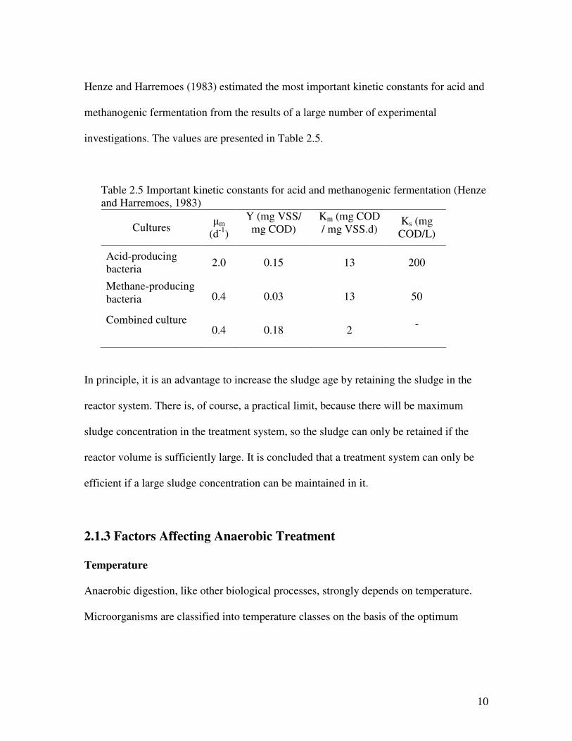
Henze and Harremoes (1983) estimated the most important kinetic constants for acid and
methanogenic fermentation from the results of a large number of experimental
investigations. The values are presented in Table 2.5.
Table 2.5 Important kinetic constants for acid and methanogenic fermentation (Henze and Harremoes, 1983)
Cultures �m
(d-1)
Y (mg VSS/ mg COD)
Km (mg COD / mg VSS.d)
Ks (mg COD/L)
Acid-producing bacteria 2.0 0.15 13 200
Methane-producing bacteria 0.4 0.03 13 50
Combined culture 0.4 0.18 2 -
In principle, it is an advantage to increase the sludge age by retaining the sludge in the
reactor system. There is, of course, a practical limit, because there will be maximum
sludge concentration in the treatment system, so the sludge can only be retained if the
reactor volume is sufficiently large. It is concluded that a treatment system can only be
efficient if a large sludge concentration can be maintained in it.
2.1.3 Factors Affecting Anaerobic Treatment
Temperature
Anaerobic digestion, like other biological processes, strongly depends on temperature.
Microorganisms are classified into temperature classes on the basis of the optimum

11
temperature and the temperature span in which the species are able to grow and
metabolize. Figure 2.2 shows the various methonogens and their growth rates.
Figure 2.2 Growth rates of methanogens (Lettinga et al., 2001).
A strong temperature effect on the maximum substrate utilization rates of
microorganisms has been observed by many researchers (Lettinga et al., 2001). In
general, lowering the operating temperature leads to a decrease in the maximum specific
growth and substrate utilization rates but it might also lead to an increased net biomass
yield (g biomass/g substrate converted) of methanogenic population or acidogenic sludge
(Lettinga et al., 2001). A drop in temperature is accompanied with a change of the
physical and chemical properties of the wastewater, which can considerably affect design
and operation of the treatment system. For instance, the solubility of gaseous compounds
increases as the temperature decreases below 200C. At low temperatures, the liquids
viscosity is also increased. Therefore, more energy is required for mixing and sludge bed
reactors become less easily mixed, particularly at low biogas production rates. Henze and
Harremoes (1983) concluded that the optimum temperature range is between 30 and 400C
12
and for temperatures below the optimum range the digestion rate decreases by about 11%
for each degree of temperature decrease, or according to the Arrhenius expression as
shown in equation 2.10
rt = r30(1.11)(t-30) (2.10)
where t = temperature in 0C and rt, r30 = digestion rate at temperature t and 300C,
respectively. The influence of temperature on anaerobic digestion is not limited by the
rate of the process; the extent of anaerobic digestion is also affected.
pH
The value and stability of the pH in an anaerobic reactor is extremely important because
methanogens can be grown at near neutral pH conditions (6.5-8.2), (Adrrianus and
Lettinga, 1994; Buyukkamaci et al., 2004). At pH values below 6.3 or above 7.8, the rate
of methanogensis decreases. Acidogenic populations are significantly less sensitive to
low or high pH values and hence acid fermentation will prevail over methanogenic
fermentation, which may result in souring of the reactor contents.
13
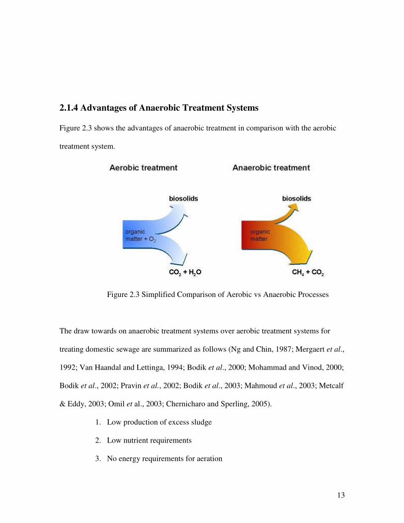
2.1.4 Advantages of Anaerobic Treatment Systems
Figure 2.3 shows the advantages of anaerobic treatment in comparison with the aerobic
treatment system.
Figure 2.3 Simplified Comparison of Aerobic vs Anaerobic Processes
The draw towards on anaerobic treatment systems over aerobic treatment systems for
treating domestic sewage are summarized as follows (Ng and Chin, 1987; Mergaert et al.,
1992; Van Haandal and Lettinga, 1994; Bodik et al., 2000; Mohammad and Vinod, 2000;
Bodik et al., 2002; Pravin et al., 2002; Bodik et al., 2003; Mahmoud et al., 2003; Metcalf
& Eddy, 2003; Omil et al., 2003; Chernicharo and Sperling, 2005).
1. Low production of excess sludge
2. Low nutrient requirements
3. No energy requirements for aeration

14
4. Produces useful products viz, methane and carbon-di-oxide gases.
5. The process can accept high organic loading rates (OLRs) since oxygen
transfer is not a limiting factor as aerobic process.
6. Anaerobic sludge can be preserved, unfed for many months without any
serious deterioration.
7. Valuable compounds like ammonia are conserved, which in specific cases
might represent an important benefit i.e. if irrigation can be applied.
2.2 Positive Perspectives for Applicability of Anaerobic Sewage
Treatment
Anaerobic treatment has also found widespread application for various industrial
wastewaters, like sugar beet, slaughterhouse, starch, brewery wastewaters, etc. The
supporting factors of sewage for the applicability of anaerobic processes are described in
the following sections.
2.2.1 Temperature in Tropical Countries
The applicability of anaerobic treatment for domestic sewage depends strongly on the
temperature of sewage. The activity of mesophilic anaerobic bacteria is at its optimum at
35°C (Van Haandel and Lettinga, 1994). At lower temperatures, bacterial activity
decreases, which results in lower treatment performances. This is the reason why in cold
climate countries, only a small separated portion of the sewage, namely the primary and
secondary sludge are treated anaerobically, however requiring heavy insulation and
heating system, while the bulk of the volume, the wastewater, is treated aerobically

15
mostly with aerators in open and closed ponds (Van Haandel and Lettinga, 1994). Figure
2.4 illustrates the critical temperature ranges grey shaded areas indicating sewage
temperatures of 12 - 15°C, the areas between the dotted lines temperature above 20°C.
Figure 2.4 World temperature zones (Van Haandel and Lettinga, 1994) Enclosed zones >20°C
Consequently anaerobic sewage treatment is primarily of interest for countries with a
tropical or sub-tropical climate, which are mostly developing countries. Bodik et al.,
(2000) studied a lab-scale upflow anaerobic filter and pilot-scale anaerobic baffled filter
to treat municipal wastewater and they found that:
1) Anaerobic wastewater treatment process is suitable for municipal or domestic
wastewater.
2) COD removal efficiency was dependant mainly on temperature and HRT. Under
low values of HRT, the removal efficiency was significantly influenced by
temperature.
16
3) The lab-scale model was operated without any technological problem. The start-
up process was realized at 23oC and was very rapid (i.e., two weeks).
4) Under ambient temperature, it was possible to obtain relatively high COD and 5
day biochemical oxygen demand (BOD5) removal efficiency.
5) Decrease in COD and BOD5 removal efficiencies were observed with decreasing
temperature.
2.2.2 Wastewater Organic Strength
Speaking of this technology, in addition to appropriate sewage temperatures, a further
precondition for effective anaerobic treatment is the organic strength of the wastewater.
The initial organic strength should be above 250 mg CODin/l, the optimum strength being
> 400 mg CODin/l (Technical Information W3e, 2001). Derin et al., (1997) mentioned
that the BOD5: COD ratio, conventionally regarded as an index of biological treatability
is calculated as 0.47. And similarly, for the COD:N ratio, a parameter closely related to
the denitrification potential, experimentally results converged to a mean value of 9.2,
practically the same as the limit below which predenitrification is favoured.
The low organic strength in domestic wastewaters (250 – 1000 mg COD/L) has to be
considered relative to the high threshold value of the methane producing bacteria. The
work done by Fukuzaki et al., (1990) shows that methanogens experienced a lower
substrate limit which they do not function properly. This so-called threshold related to
undissociated acetic acid, the true substrate for acetogenic methanogens. This could
easily result in residual volatile fatty acids (VFA) levels which are high with respect to
the levels of the incoming sewage and thus implicate low removal efficiency.

17
Consequently, anaerobic treatment is of interest only for relatively concentrated domestic
wastewaters (COD > 500 mg/L) unless in the case of highly adapted Methanotrix sludges.
Sewage characteristics which can have direct implications on the anaerobic process are
summarized in Table 2.6.
Table 2.6 Composition ranges of municipal wastewater for industrialized countries (Mergaert et al., 1992 and Metcalf & Eddy, 2003)
Characteristics Average
Total Chemical Oxygen Demand (tCOD), mg/L
500
Total Kjeldahl Nitrogen (TKN), mg/L 50
Ammonical Nitrogen (NH4+-N), mg/L 25-40
Volatile acids as acetic acid, mg/L 40
Sulphate, (SO42- ), mg/L 75
Lipids, mg/L 40-100 (Alves et al., 2001)
2.2.3 Total Kjeldahl Nitrogen (TKN) and Ammonical Nitrogen (NH4+-N)
The NH4+ concentration in domestic wastewater is in the range of 25 – 40 mg/L
(Mergaert et al., 1992). This represents no problem for anaerobic treatment. The ratio of
COD: N of 100:10 for domestic wastewater, is also higher than the minimum amount of
nitrogen necessary for normal anaerobic sludge growth (ratio COD: N = 100:1.25)
(Mergeart et al., 1992). The COD: N: P ratio of 100:13:2 indicated the high treatability of
the wastewater by an anaerobic process. Panswad and Komolmethee (1997) indicated
18
that the optimum nutrient ratio given as COD: N: P was 190 to 350:5:1. Anaerobic
treatment however being feasible up to a ratio of 100:5:1. This shows that the average
sewage composition meets these requirements.
2.2.4 Fatty Acids
The relatively low levels of VFA coupled to the alkalinity of domestic wastewater make
it unlikely that inhibition by VFA has to be a concern. Long chain fatty acids, e.g. from
soaps, appear to be more toxic (50% inhibition at 500 mg/L; Mergeart et al., 1992) and
can sometimes be present in domestic waste as a result of certain seasonal household
habits. This aspect necessitates further research.
2.2.5 pH
Kobayashi et al. (1983) studied a laboratory scale anaerobic filter for treatment of low
strength domestic wastewater which had pH in the range of 5.72 to 8.95 with an average
of 7.51. In addition to that it was reported that the pH of treated domestic wastewater was
in range of 6.85 to 8.2 with an average of 7.28. Methanogens can be grown at near
neutral pH conditions, defined as 6.5 - 8.2, which is a normal pH value of sewage
(Buyukkamaci et al., 2004). The average sewage composition meets these requirements.
2.2.6 Sulfate
The sulfate levels in domestic wastewater are relatively low so it is unlikely that the
critical value of 50 mg/L hydrogen sulphide (H2S). Since the optimal temperature for

19
sulfate reducing bacteria (SRB) is between 30 and 350C and thus a little lower than the
optimal temperature for methane producing bacteria (MPB) (between 35 and 450C)
(Mergeart et al., 1992), it is possible that at sewage temperatures of 10 - 200C the SRB
tend to out compete the MPB so that a major part of the COD is consumed for sulfate
reduction with contaminant production of corrosive sulfides. Hence, direct anaerobic
treatment of municipal wastewater will necessitate post-treatment. MetCalf and Eddy
(2003) indicated that the concentration of oxidized sulfur compounds in the influent
wastewater to an anaerobic treatment process is important, as high concentrations can
have a negative effect on anaerobic treatment. As mentioned earlier sulfate reducing
bacteria compete with the methanogenic bacteria for COD and thus can decrease the
amount of methane gas production. While low concentrations of sulfide (less than 20
mg/L) are needed for optimal methanogenic activity, higher concentrations can be toxic.
Methanogenic activity was reported to decrease by 50% or more at H2S concentrations
ranging from 50 to 250 mg/L (Mergeart et al., 1992).
2.2.7 Toxicants
Control of toxicants is also an important issue in the anaerobic system. Apart form the
hydrogen ion concentration, several other compounds affect the rate of anaerobic
digestion, even at very low concentration, such as heavy metals and chloro-organic
compounds at inhibitory concentrations is unlikely in sewage.
2.2.8 Flow rate of the wastewater

20
Municipal wastewater is characterized by strong fluctuations in organic matter,
suspended solids and flow rate. Concentrations of BOD, COD and TSS can vary with a
factor of 2-10 in half an hour to a few hours (Mergeart et al., 1992). Flow rate
fluctuations of domestic wastewater depend mainly on the size of population (the larger
the population, the smaller the variation) and the sewer type (combined sewers have
much higher fluctuations, due to receiving rain and run off water). Daily flow rate
variations: the variation in flow tends to follow a diurnal pattern. The wastewater
discharge curve closely follows the water consumption curve, but with a lag of several
hours (Metcalf and Eddy, 2003).
2.3 Application of Anaerobic Treatment Technology for Municipal
Wastewater 2.3.1 Perspectives of Anaerobic-Aerobic Systems:
In tropical countries sewage treatment, the aerobic processes (CAS (Conventional
Activated Sludge) and MBR (Membrane Bioreactor) in the near future) have proven to be
effective in producing high quality effluent to meet the discharge and water reclamation
standards. However, aerobic systems are by nature, net energy consuming process,
mainly due to the aeration requirements to sustain the aerobic microbial populations.
Anaerobic process, on the other hand, does not require aeration and produces methane
gas as a by-product during biodegradation of the complex organics, which can be utilized
as fuel for energy production. Coupled by other advantages such as low sludge
production, natural in process, simplicity in operation makes anaerobic technology
environmentally friendly, cost-effective and economical.

21
2.3.2 Necessity of Aerobic Post-treatment Systems:
However, anaerobic processes are not very efficient when it comes to nutrients removal
(such as nitrogen and phosphorus). Thus aerobic processes are still required as a
polishing step on the anaerobic effluent to achieve the required standards for discharge or
for further water reuse (Kobayashi et al., 1983). Whilst anaerobic processes have several
advantages, it is important to realise that their treatment capacity is not sufficient.
Treatment of simple organic material is reasonable, but for any additional treatment
requirement, post-treatment processes are required. Therefore, in low- and middle-
income countries where pollution should be of most concern, the use of anaerobic
treatment in isolation is not sufficient.
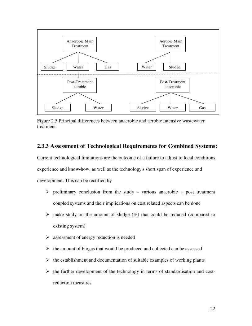
Under “real life” conditions in developing countries, typical full scale process
combinations (as presented in Figure 2.5) are however rarely entirely realised. Instead,
often only the main treatment steps (aerobic wastewater treatment without a sludge
digestion or anaerobic UASB treatment of sludge and wastewater without a post-
treatment of the wastewater) are put in place in order to reduce the most severe
environmental effects. Accordingly, post-treatment steps shown in Figure 2.5, below the
dotted line are often not realised in developing countries as yet.
22
Figure 2.5 Principal differences between anaerobic and aerobic intensive wastewater treatment 2.3.3 Assessment of Technological Requirements for Combined Systems: Current technological limitations are the outcome of a failure to adjust to local conditions,
experience and know-how, as well as the technology's short span of experience and
development. This can be rectified by
� preliminary conclusion from the study – various anaerobic + post treatment
coupled systems and their implications on cost related aspects can be done
� make study on the amount of sludge (%) that could be reduced (compared to
existing system)
� assessment of energy reduction is needed
� the amount of biogas that would be produced and collected can be assessed
� the establishment and documentation of suitable examples of working plants
� the further development of the technology in terms of standardisation and cost-
reduction measures
Anaerobic Main Treatment
Aerobic Main Treatment
Sludge
Post-Treatment aerobic
Sludge Water Sludge Water Gas
Post-Treatment anaerobic
Water Gas Water Sludge

23
� practical research and development in the areas of preliminary and post-treatment,
pathogen removal emission and odour control, gas utilisation, sludge storage,
small and medium-sized systems
� rehabilitation and improvement of existing plants
2.4 Progress of Anaerobic Treatment Technology for Municipal Wastewater
The first application of anaerobic digestion for sewage treatment is presumably the air-
tight chamber developed by the end of last century in France by M. Mouras (Van
Hanndel and Lettinga, 1994). Around the change of the century, several new anaerobic
treatment systems were developed. In 1935 world’s largest sewage treatment plant with
imhoff tanks was constructed in Chicago (Van Hanndel and Lettinga, 1994).
In the following decades, anaerobic treatment of sewage became less popular than
aerobic sewage treatment systems such as the trickling filter and activated sludge
processes. This decreased application of anaerobic treatment was mainly due to higher
removal efficiency of organic matter achieved in the aerobic systems. Well operated
aerobic systems would remove 90 – 95 percent of the biodegradable organic matter from
raw sewage. In the early anaerobic systems the removal was based on the settling of
suspended organic matter. As only a fraction of the influent organic matter is settleable
(one third to one half), the maximum removal efficiency in these systems did not exceed
30-50 percent of the biodegradable matter, depending on the nature of the sewage and the
settling efficiency (Van Hanndel and Lettinga, 1994).
The low removal efficiency of the primary treatment systems must be attributed to a
fundamental design failure. As there is little, if any, contact between the anaerobic micro-

24
organisms in the system and the non-settleable part of the organic matter in the influent,
the main part of the dissolved or hydroylsed organic matter cannot be metabolized and
leaves the treatment system. A very important aspect is the contact between the
microorganisms and the wastewaters. The importance of a sufficient contact between
influent organic matter and the bacterial population was not recognized at that time. The
resulting relatively poor performance of anaerobic systems led to the belief that they were
inherently inferior to aerobic systems, an opinion which often still persists today.
However, in the mean time, it has been demonstrated that a properly designed modern
anaerobic treatment system can attain a high removal efficiency of biodegradable organic
matter, even at very short retention times.
A breakthrough in the design of anaerobic treatment systems came about with the
development of ‘modern’ or high rate systems. All modern high rate anaerobic treatment
systems are based on various kinds of sludge immobilization principle in order to retain
as much sludge as possible. The different types of anaerobic treatment systems have been
applied to a great variety of industrial wastes, but so far the anaerobic treatment concept
is rarely used for sewage so experimental information is scarce. In fact, experimental
results of anaerobic sewage treatment in modern systems are restricted to the use of the
anaerobic filter (AF), fluidized and expanded bed (FB/EB) and uplfow anaerobic sludge
blanket (UASB). Comparison of process behaviour of all these three different modern
high rate anaerobic processes is listed in Table 2.7.

25
Table 2.7 Comparison of different anaerobic process behaviour
Characteristic behaviour UASB AF FB/EB
Reactor start-up - - -
Biomass accumulation * + *
Liquid-phase mixing - + *
Robustness against hydraulic shocks - * *
Robustness against organic shocks + + +
Insensitivity to suspended solids - + *
Insensitivity to clogging * - *
Risk for biomass flotation - + +
Demand for reactor control + + -
- Unfavourable + Favourable * Very favourable
The upflow anaerobic filter system can suffer from clogging (channeling) problems. In
UASB reactors, channeling problems occur only at low loading rates and when a poor
feed-inlet distribution system has been installed in the reactor. In fluidized-bed reactors, a
good contact between micro-organisms and wastewater is guaranteed and provided with a
sophisticated feed-inlet distribution system. On the other hand, fluidized bed reactors
require a high recycle factor, which may result in a distinct drop in substrate utilization
rate by the active biomass because of the relatively low substrate levels prevailing in the
reactor. In attached film processes, the maximum sludge retention depends mainly on the
surface area for sludge attachment, the film thickness, the space occupied by the carrier
material and the extent to which dispersed sludge aggregates are retained. In upflow

26
anaerobic filters the voidage of the packing material is a factor of prime importance with
regard to sludge retention (Van Haandel and Lettinga, 1984).
2.5 Upflow Anaerobic Filter
Biofilm, or fixed film, reactors depend on the natural tendency of mixed microbial
populations to adsorb to surfaces and to accumulate in biofilms. Adsorbed
microorganisms grow, reproduce, and produce extracellular polymeric substances that
frequently extend from the cell, forming the gelatinous matrix called a biofilm. Jimeno et
al (1990) defined that bacterial attachment is mediated by polymeric material, primarily
polysaccharide, which extended from the cell to form a tangled mass of fibers, termed a
glycocalyx. The entire deposit is called a biofilm. The accumulation and persistence of a
biofilm is the net result of several physical and biological processes that occur
simultaneously, although their relative rates will change through the various stages. The
mixing in these reactors is typical of plug flow (James and William, 1990).
In the upflow anaerobic packed-bed reactor the packing is fixed and the wastewater flows
up through the interstitial spaces between the packing and biogrowth. While the first
upflow anaerobic packed-bed processes contained rock, a variety of designs employing
synthetic plastic packing are used currently. A large portion of the biomass responsible
for treatment in the upflow attached growth anaerobic processes is loosely held in the
packing void spaces and not just attached to the packing material (Metcalf and Eddy,
2003).
27
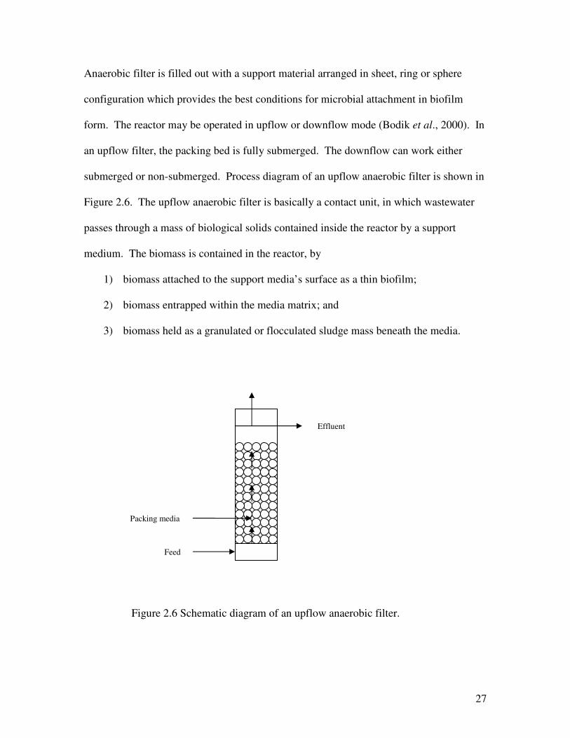
Anaerobic filter is filled out with a support material arranged in sheet, ring or sphere
configuration which provides the best conditions for microbial attachment in biofilm
form. The reactor may be operated in upflow or downflow mode (Bodik et al., 2000). In
an upflow filter, the packing bed is fully submerged. The downflow can work either
submerged or non-submerged. Process diagram of an upflow anaerobic filter is shown in
Figure 2.6. The upflow anaerobic filter is basically a contact unit, in which wastewater
passes through a mass of biological solids contained inside the reactor by a support
medium. The biomass is contained in the reactor, by
1) biomass attached to the support media’s surface as a thin biofilm;
2) biomass entrapped within the media matrix; and
3) biomass held as a granulated or flocculated sludge mass beneath the media.
Figure 2.6 Schematic diagram of an upflow anaerobic filter.
Effluent
Feed
Packing media

28
Ramakrishnan and Gupta (2006) indicated that start-up of anaerobic reactors is more time
consuming and is subjected to disturbances more than that of aerobic reactors. The start-
up of the anaerobic process is still considered a major area of research. Many researchers
have reported long start-up periods of 2 - 3 months to 1 year (or even more) for the
anaerobic reactors. Accordingly, Punal et al. (2000) mentioned that long duration of start-
up period is a major drawback of the anaerobic wastewater treatment systems.
Considerable efforts have been made to study the granulation process but the mechanism
involved in the formation of granulation sludge is still unknown. A better understanding
of the factors affecting biomass aggregation and adhesion, the two main mechanisms of
biomass retention, could make the start-up more efficient and rapid. A feeding strategy,
consisting of maintaining a low nitrogen concentration in the influent during the first two
weeks followed by nitrogen balanced feed, is proposed in order to quicken the start-up of
anaerobic filters. In addition, Subbiah (1997) reported that the start-up period required
was about 54 days before the upflow anaerobic filter achieved steady state.
Low upflow velocities are generally used to prevent washing out the biomass as
mentioned by Metcalf and Eddy (2003). Jimeno et al. (1990) reported that the C:N:P ratio
of 100:2:1 is optimal for the start-up of anaerobic fixed-film reactors.
As the wastewater passes over the biomass, the soluble organic compounds contained in
the influent wastewater, which is in contact with the biomass, are being diffused through
the biofilm or the granular sludge. They are then converted into intermediate and final

29
products, specifically methane and carbon dioxide. The effluent from the anaerobic filter
is usually well clarified and has relatively low concentration of organic matter.
Anaerobic filter can have several shapes, configurations and dimension, provided that the
flow is well distributed over the bed. In full scale systems, anaerobic filters are usually
present either in cylindrical or rectangular shape. The diameters of the tanks vary from 6
to 26 m and their heights from 3 to approximately 13 m. The volumes of the reactors
vary from 100 to 10,000 m3. Packing material may be in the entire depth or, for hybrid
designs, only in the upper 50 to 70 percent (Van Hanndal & Lettinga, 1994).
2.5.1 Origin and Development of Anaerobic Filter
The first works on anaerobic filter dated back to the late 1960s and they have had a
growing application since that time for treatment of both domestic wastewater and a
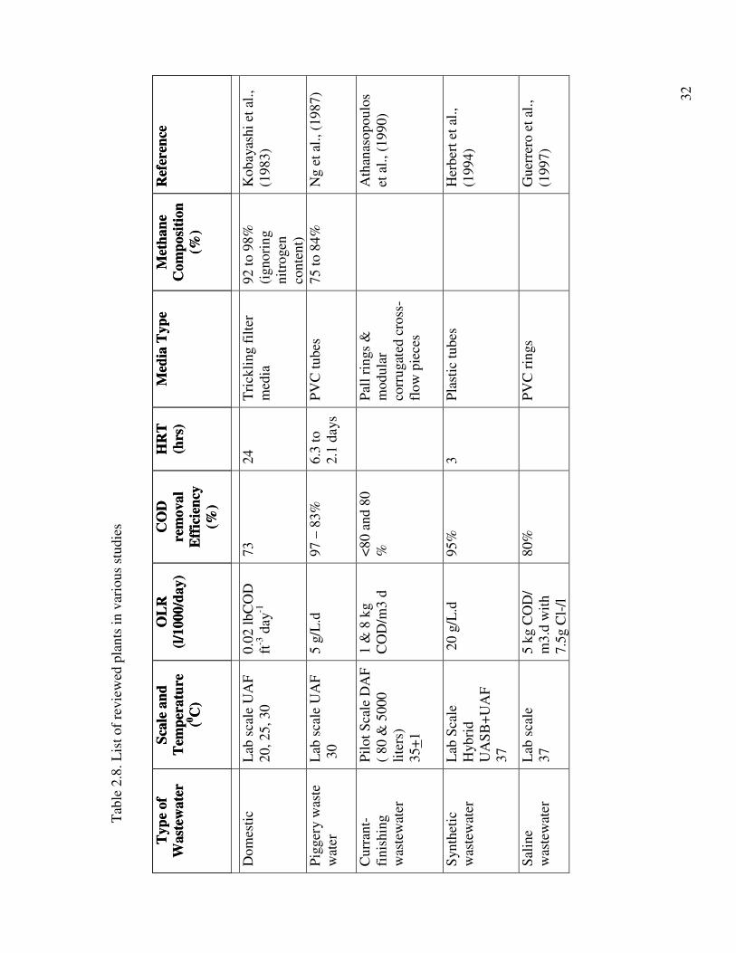
diversity of industrial effluents. Table 8 shows the list of various anaerobic filters studied
for different types of wastewater.
Two important developments in the application of anaerobic processes to lower strength
wastewaters are the development of the anaerobic contact process by Schroepfer et al.
(1955); Schroepfer and Ziemke (1959) and the development of the anaerobic filter by
Coulter et al. (1957) and Young and McCarty (1968). The key concept of both processes
relates to the ability to control mean cell retention time (MCRT) independently of
hydraulic retention time. This feature permits anaerobic treatment at lower temperatures
than previously thought possible or economical. Ng and Chin (1987) stated that without
increasing MCRT independently of hydraulic retention time, very large reactor volumes

30
are required, making anaerobic treatment techniques too costly. Since heating is not
required at tropical climate, low strength wastes, which produce only small quantities of
gas per unit volume of waste treated, can be effectively treated by the anaerobic filter or
anaerobic contact process. In addition, Kobayashi et al. (1983) stated that the filter
performance at 25 and 350C was not significantly different.
The modern anaerobic filter was reported as early as in 1968 by Young and McCarty
(Van Hanndal & Lettinga, 1994). They reported a completely submerged, 12-L lab-scale
reactor which was filled with 1.0 to 1.5 inch quartzite stone. The findings of Young and
McCarty (1968) are as follows:
1) the anaerobic filter is ideal for the treatment of soluble wastewaters;
2) accumulation of biological solids in the anaerobic filter leads to long solids
retention times (SRTs) and low effluent total suspended solids (TSS) and
3) low strength wastes were successfully treated at the temperature of 25oC because
of long SRTs.
In addition to the initial studies done by Young and McCarty (1968), anaerobic filter was
used to treat different types of wastewater by numerous researchers. Anaerobic filter is
being used for treating high strength industrial wastewater for a long time. Ng and Chin
(1987) had used a lab-scale anaerobic filter to treat piggery wastewater successfully. And
Herbert et al. (1994) studied a lab-scale hybrid system of UASB and anaerobic filter to
treat synthetic wastewater comprising milk and sucrose with balanced nutrients and trace
metals. It was reported that a hybrid system of UASB and anaerobic filter could achieve
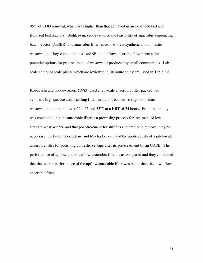
31
95% of COD removal, which was higher than that achieved in an expanded bed and
fluidized bed reactors. Bodik et al. (2002) studied the feasibility of anaerobic sequencing
batch reactor (AnSBR) and anaerobic filter reactors to treat synthetic and domestic
wastewater. They concluded that AnSBR and upflow anaerobic filter seem to be
potential options for pre-treatment of wastewater produced by small communities. Lab
scale and pilot scale plants which are reviewed in literature study are listed in Table 2.8.
Kobayashi and his coworkers (1983) used a lab-scale anaerobic filter packed with
synthetic high surface area trickling filter media to treat low strength domestic
wastewater at temperatures of 20, 25 and 35oC at a HRT of 24 hours. From their study it
was concluded that the anaerobic filter is a promising process for treatment of low
strength wastewaters, and that post-treatment for sulfides and ammonia removal may be
necessary. In 1998, Chernicharo and Machado evaluated the applicability of a pilot-scale
anaerobic filter for polishing domestic sewage after its pre-treatment by an UASB. The
performance of upflow and downflow anaerobic filters was compared and they concluded
that the overall performance of the upflow anaerobic filter was better than the down flow
anaerobic filter.
32
Tab
le 2
.8. L
ist o
f rev
iew
ed p
lant
s in
var
ious
stu
dies
Typ
e of
W
aste
wat
er
Scal
e an
d T
empe
ratu
re
(0 C)
OL
R
(l/10
00/d
ay)
CO
D
rem
oval
E
ffic
ienc
y (%
)
HR
T
(hrs
) M
edia
Typ
e M
etha
ne
Com
posi
tion
(%)
Ref
eren
ce
Dom
estic
La
b sc
ale
UA
F 20
, 25,
30
0.02
lbC
OD
ft
-3 d
ay-1
73
24
T
rick
ling
filte
r m
edia
92
to 9
8%
(ign
orin
g ni
trog
en
cont
ent)
Kob
ayas
hi e
t al.,
(1
983)
Pigg
ery
was
te
wat
er
Lab
scal
e U
AF
30
5 g/
L.d
97 –
83%
6.
3 to
2.
1 da
ys
PVC
tube
s 75
to 8
4%
Ng
et a
l., (1
987)
Cur
rant
-fi
nish
ing
was
tew
ater
Pilo
t Sca
le D
AF
( 80
& 5
000
liter
s)
35+ 1
1 &
8 k
g C
OD
/m3
d <8
0 an
d 80
%
Pall
ring
s &
m
odul
ar
corr
ugat
ed c
ross
-fl
ow p
iece
s
A
than
asop
oulo
s et
al.,
(199
0)
Synt
hetic
w
aste
wat
er
Lab
Scal
e H
ybri
d U
ASB
+UA
F 37
20
g/L.
d 95
%
3 Pl
astic
tube
s
Her
bert
et a
l.,
(199
4)
Salin
e w
aste
wat
er
Lab
scal
e 37
5
kg C
OD
/ m
3.d
with
7.
5g C
l-/l
80%
PVC
ring
s
Gue
rrer
o et
al.,
(1
997)
Typ
e of
W
aste
wat
er
Scal
e an
d T
empe
ratu
re
(0 C)
OL
R
(l/10
00/d
ay)
CO
D
rem
oval
E
ffic
ienc
y (%
)
HR
T
(hrs
) M
edia
Typ
e M
etha
ne
Com
posi
tion
(%)
Ref
eren
ce

33
Was
tew
ater
fr
om c
offe
e pr
oces
sing
pl
ant
Pilo
t sca
le
1.
89 k
g C
OD
/m3.
d 77
.2%
22
V
olca
nic
rock
s
(Bel
lo-M
endo
za
and
Cas
tillo
-R
iver
a, (1
998)
Dom
estic
La
b sc
ale
Mul
tista
ge U
AF
97
to 8
6%
4 da
ys
to 8
h W
aste
tyre
tube
Rey
es e
t al.,
(1
999)
Mun
icip
al
was
tew
ater
La
b sc
ale
&
Pilo
t sca
le
23, 1
5, 9
64
87
90
66
8 15
23
24
Plas
tic fi
lling
s
Bod
ik e
t al.,
(2
000)
Dom
estic
La
b sc
ale
24+1
63
0.5
Ret
icul
ated
Po
lyur
etha
ne
Foam
(RPF
)
E
lmitw
alli
et a
l.,
(200
0)
Synt
hetic
Su
bstr
ate
Lab
Scal
e
24
77
6
Plas
tic m
ater
ial
B
odik
et a
l.,
(200
2)
Dom
estic
La
b Sc
ale
AF
+ A
H
13
81
4
Ret
icul
ated
Po
lyur
etha
ne
Foam
(RPF
)
70.7
+ 2.9
E
lmitw
alli
et a
l.,
(200
2a)

34
In addition, Athanasopoulos et al. (1990) studied two down flow anaerobic filters with
different plastic media of the same specific area, treating currant-finishing wastewater
and concluded that down flow anaerobic filters had a lower performance compared with
other high-rate anaerobic reactors, UAF and UASB.
Bodik et al. (2000) studied a lab-scale upflow anaerobic filter and pilot-scale anaerobic
baffled filter to treat municipal wastewater and their research findings confirmed that
anaerobic wastewater treatment process was suitable for municipal or domestic
wastewater and the pilot-scale reactor worked during the whole experiments without any
technological problems; no significant changes of pH, VFA were observed in the
anaerobic reactor.
In addition, Fatma and Michael (2003) developed a dynamic mathematical model to
understand the applicability of anaerobic treatment for low strength wastewater. The
model had served as a predictive tool for treatment efficiency and gas production.
Advantages of Upflow Anaerobic Filter
Ng et al. (1987) stated that anaerobic processes are usually limited by the low growth rate
of the methanogens. Due to this limitation, conventional suspended-growth anaerobic
treatment systems require lengthy retention times and thus large reactor volume. The
advantages of anaerobic filter (an attached-growth system) over a suspended-growth
anaerobic high-rate reactor are as follows:

35
1) Biofilm reactors are especially useful when slow growing organisms have to be
kept in wastewater treatment (Bodik et al., 2003).
2) It has relatively good load fluctuation resistance (Kobayashi et al., 1983; Nebot
el al., 1995; Bodik et al., 2000; Francisco Omil et al., 2003).
3) In anaerobic filter, bacteria adhere to support media so that, even at relatively
high hydraulic loads (which would wash bacterial biomass out of conventional
suspended growth digesters), the filter retains the bacteria (Young and McCarty,
1968).
4) The amount of produced sludge is smaller and settleability of sludge is good
(Bodik et al., 2000).
5) Due to the efficient biomass retention, long sludge ages and more compact
reactors can easily be achieved (Kobayashi et al., 1983; Bodik et al., 2003).
6) Sludge is not returned, unlike the anaerobic activated sludge process (Bodik et al.,
2000). Therefore cost of energy for sludge returning is not necessary.
7) Suitable for treatment of low soluble organic wastewater (Bodik et al., 2000).

36
Disadvantages of Upflow Anaerobic Filter
However, anaerobic filter has some drawbacks too. The disadvantages of anaerobic filter
are as follows (Bodik et al., 2000):
1) channeling can occur, i.e. formation of preferential paths of liquid flow through
the reactor.
2) dead-zone formation caused by sludge compaction or clogging of matrix
interstitial spaces by solids.
3) clogging of poorly designed distribution systems.
Packing Media
The purpose of packing medium is to retain solids inside the reactor, either by the biofilm
formed on the surface of the packing medium or by the retention of solids in the
interstices of the medium or below it. The main purposes of the packing media are as
follows:
1) acting as a device to separate solids from liquid;
2) helping to promote a uniform flow in the reactor;
3) improving the contact between the components of the influent wastewater and the
biological solids contained in the reactor;
4) allowing the accumulation of high amount of biomass, with a consequently
increased solids retention time; and
5) acting as a physical barrier to prevent solids from being washed out from the
treatment system.

37
Several types of materials have been used as packing media in biological reactors,
including quartz, ceramic blocks, oysters and mussel shells, limestone, plastic rings,
hollow cylinders, PVC modular blocks, granite, polyethylene balls and bamboo. The
packing media have been designed to occupy from the total depth of the reactor to
approximately 50 to 70% of the height of the reactor. There are different types of plastic
packing media available in the market, ranging from corrugated rings to corrugated plate
blocks. The specific surface areas of these plastic materials usually range from 100 to
200 m2/m3. Although some types of packing media are more efficient than others in the
retention of biomass, the final choice will depend on the specific local conditions,
economic considerations and operational factors. The requirements for good packing
media of anaerobic filter are listed in Table 2.9.
Elmitwalli et al. (2000) indicated that specific surface area, porosity, surface roughness,
pore size and orientation of the packing material were important factors influencing the
anaerobic filter reactor performance. High surface area and porosity, large pore size and
rough surface area for packing material improved performance of an AF reactor.
Subsequently, Mohammad (2000) stated if an excessively small medium is employed
AFs may suffer from blockages and to minimize blockages, filter media tend to have
relatively large diameters (>20 mm). The surface roughness of packing filter media and
degree of porosity, in addition to pore size, affect the rate of colonization by bacteria
(Stronach et al., 1986).

38
Table 2.9. Requirements of packing media for an anaerobic filter.
Requirement Objective
Structural resistance Support their own weight and the weight of the biological
solids attached to the surface
Biological and
chemical inertness
Allow no reaction between the bed and the microorganisms
Sufficient light Avoid the need for expensive, heavy structures, and allow the
construction of relatively higher filters, which implies a
reduced area necessary for the installation of the system
Large specific area Allow the attachment of a larger quantity of biological solids
High porosity Allow a larger free area available for the accumulation of
bacteria and reduce the possibility of clogging
Enable the accelerated
colonization of
microorganisms
Reduce the start-up time of the reactor
Present a rough surface
and a non-flat format
Ensure good attachment and high porosity
Low cost Make the process feasible, not only technically, but also
economically
39
CHAPTER 3 MATERIALS AND METHODS
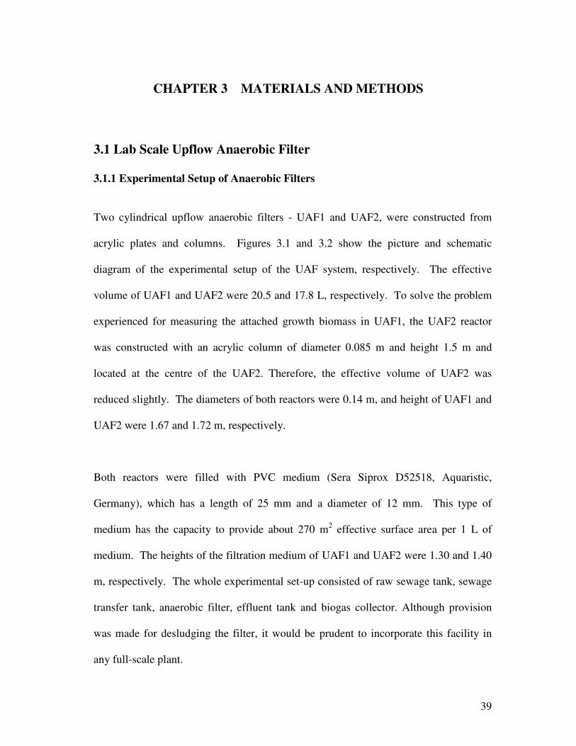
3.1 Lab Scale Upflow Anaerobic Filter 3.1.1 Experimental Setup of Anaerobic Filters
Two cylindrical upflow anaerobic filters - UAF1 and UAF2, were constructed from
acrylic plates and columns. Figures 3.1 and 3.2 show the picture and schematic
diagram of the experimental setup of the UAF system, respectively. The effective
volume of UAF1 and UAF2 were 20.5 and 17.8 L, respectively. To solve the problem
experienced for measuring the attached growth biomass in UAF1, the UAF2 reactor
was constructed with an acrylic column of diameter 0.085 m and height 1.5 m and
located at the centre of the UAF2. Therefore, the effective volume of UAF2 was
reduced slightly. The diameters of both reactors were 0.14 m, and height of UAF1 and
UAF2 were 1.67 and 1.72 m, respectively.
Both reactors were filled with PVC medium (Sera Siprox D52518, Aquaristic,
Germany), which has a length of 25 mm and a diameter of 12 mm. This type of
medium has the capacity to provide about 270 m2 effective surface area per 1 L of
medium. The heights of the filtration medium of UAF1 and UAF2 were 1.30 and 1.40
m, respectively. The whole experimental set-up consisted of raw sewage tank, sewage
transfer tank, anaerobic filter, effluent tank and biogas collector. Although provision
was made for desludging the filter, it would be prudent to incorporate this facility in
any full-scale plant.

40
Figu
re 3
.1 P
ictu
re o
f Upf
low
Ana
erob
ic F
ilter
s

41
Fi
gure
3.2
Sch
emat
ic d
iagr
am o
f UA
F ex
peri
men
tal s
et u
p
Raw
Sew
age
Tan
k E
fflu
ent T
ank
PH C
ontro
ller
A
F R
eact
or
Stirr
er
Eff
luen
t
Slud
ge
Sam
plin
g Po
rts
Dra
inag
e
Bio
gas
Flow
Aci
d W
ater
Floa
ting
Cov
er
Gas
C
olle
ctor
w
ith
Cou
nter
-W
eigh
ts
Bio
gas
Filtr
atio
n M
ediu
m
Mag
netic
Stir
rer
Influ
ent P
ump
Stirr
er
Tra
nsfe
r Pum
p
Stirr
er
Tem
pera
ture
C
ontr
ol S
yste
m
Sew
age
Tra
nsfe
r T
ank
pH P
robe
Aci
d W
ater
Floa
ting
Cov
er
Gas
C
olle
ctor
w
ith
Cou
nter
-W
eigh
ts
Cau
stic
42
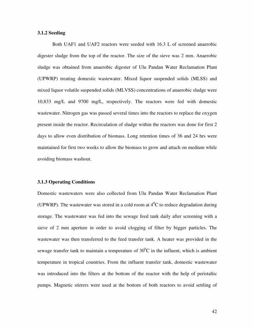
3.1.2 Seeding
Both UAF1 and UAF2 reactors were seeded with 16.3 L of screened anaerobic
digester sludge from the top of the reactor. The size of the sieve was 2 mm. Anaerobic
sludge was obtained from anaerobic digester of Ulu Pandan Water Reclamation Plant
(UPWRP) treating domestic wastewater. Mixed liquor suspended solids (MLSS) and
mixed liquor volatile suspended solids (MLVSS) concentrations of anaerobic sludge were
10,833 mg/L and 9700 mg/L, respectively. The reactors were fed with domestic
wastewater. Nitrogen gas was passed several times into the reactors to replace the oxygen
present inside the reactor. Recirculation of sludge within the reactors was done for first 2
days to allow even distribution of biomass. Long retention times of 36 and 24 hrs were
maintained for first two weeks to allow the biomass to grow and attach on medium while
avoiding biomass washout.
3.1.3 Operating Conditions
Domestic wastewaters were also collected from Ulu Pandan Water Reclamation Plant
(UPWRP). The wastewater was stored in a cold room at 40C to reduce degradation during
storage. The wastewater was fed into the sewage feed tank daily after screening with a
sieve of 2 mm aperture in order to avoid clogging of filter by bigger particles. The
wastewater was then transferred to the feed transfer tank. A heater was provided in the
sewage transfer tank to maintain a temperature of 300C in the influent, which is ambient
temperature in tropical countries. From the influent transfer tank, domestic wastewater
was introduced into the filters at the bottom of the reactor with the help of peristaltic
pumps. Magnetic stirrers were used at the bottom of both reactors to avoid settling of
43
suspended solids present in the domestic wastewater. Two pH probes were provided to
monitor the pH of effluent from the reactors in order to maintain the pH between 6.8 and
7.2. Since higher concentrations of Volatile Fatty Acids (VFA) accumulation was
expected in the reactors, stand by alkaline dosage arrangement was set up to increase the
pH. A biogas collector was provided for each UAF to collect the biogas produced from
each reactor. They are floating covered gas collectors with counter-weights. The water
inside the biogas cylinder containers were acidified to pH of around 4. There was no
effluent recirculation in both UAFs and no intended sludge wasting throughout the
operation. The operating conditions maintained for the anaerobic filters were as follows:
pH - 6.8 to 7.2
Temperature -30 0C
HRTs -24, 16, 12, 8, 6, and 4hrs
Influent, effluent, biomass and biogas samples were collected from the reactors and
analyzed.
3.2 Analytical Methods
Performance of anaerobic filters were monitored by analyzing suspended solids (SS),
volatile suspended solids (VSS), total chemical oxygen demand (tCOD), soluble
chemical oxygen demand (sCOD), five-day total biochemical oxygen demand (tBOD5),
five-day soluble biochemical oxygen demand (sBOD5), alkalinity, volatile fatty acids
(VFAs), anions, cations of influent and effluent, mixed liquor suspended solids (MLSS),
mixed liquor volatile suspended solids (MLVSS), gas production and gas composition.
44
These parameters were tested in accordance with the Standard Methods listed for water &
wastewater (APHA, 1998).
3.2.1 Total Suspended Solids (TSS) and Volatile Suspended Solids (VSS)
Total suspended solids and volatile suspended solids concentrations were determined
according to the method specified in the Standard Methods (APHA, 1998). For TSS
measurement, the sample was dried in an oven (MEMMERT ULM 6, Schmidt Scientific)
at 105oC for 1 hour. For VSS measurement, the sample was further burned in a furnace
(Thermolyne 48000, Omega Medical Scientific) at 550oC for 20 minutes.
3.2.2 Chemical Oxygen Demand (COD)
The closed reflux method (Block heater: HACH COD Heater, Model 16500-10) in
accordance with the Standard Methods (APHA, 1998) was used to measure COD.
3.2.3 Biochemical Oxygen Demand (BOD)
The BOD measurements were done in accordance with the Standard Methods (APHA,
1998). The dissolved oxygen (DO) concentration in the samples was monitored with a
DO meter (YSI Model-58, YSI Integrated Systems & Services, United States of America).

45
3.2.4 Biogas Composition
The biogas composition was measured using the gas chromatography (Shimadzu GC-
17A, Shimadzu Scientific Instruments, United States of America) unit with packed
column (80/100 PORAPAK, 2m X 1/8 in., SUPELCO, United States of America) using
Argon as the carrier gas. Calibration was performed using 100 µl of standard gas
comprising 25% H2, 25% N2, 10% CH4 and 40% CO2. One hundred microliter of sample
was injected in each run and the experiment was repeated 3 times.
3.2.5 Total Nitrogen (TN)
TN concentrations of the samples were measured using Shimadzu TOC analyzer
(Shimadzu TOC-VCSH, Shimadzu Scientific Instruments, United States of America) and a
TN measuring unit (Shimadzu TNM-1, Shimadzu Scientific Instruments, United States of
America).
3.2.6 Total Phosphorus (TP)
The sample was first pre-treated using test kit from HACH (total phosphate, 0-3.5 mg/L,
reagent set 27426-45, HACH Company, United States of America). The total
phosphorus concentration was then analyzed with a spectrophotometer (HACH
DR/4000U, HACH Company, United States of America).

46
3.2.7 Volatile Fatty Acid (VFA)
The Flame Ionization Detector (FID) (Shimadzu GC-2010, Shimadzu Scientific
Instruments, United States of America) with capillary column (25 m x 0.32 mm, HP-
FFAP, Agilent Technologies Inc., United States of America) was used to detect VFA
concentration of the influent sewage and anaerobic treated effluent samples. Acetic,
propionic, butyric and n-valeric acid were prepared as standards for calibration up to
concentrations of 200 mg/L. Nine parts of sample was mixed with 1 part of formic acid
before injecting into the unit for analysis. An injection volume of 0.2 ml at column
temperature of 150oC was used and run time for each sample was 10 minutes.
VFAs were analysed using a gas chromotogrpah (GC, Chrompack CP 9000, Varian, Inc.
Scientific Instruments, United States of America) equipped with a flame ionization
detector. The VFA analytic procedure was in accordance with that described by
Buyukkamaci et al. 2004. The volatile acids in the sample were separated and quantified
as free acids by using a capillary column (Nukol, 30 m X 0.25 mm i.d., 0.25um film;
Supelco Cat. No: 4-6875, SUPELCO, United States of America). Nitrogen gas was used
as carrier gas with a rate of 20 cm s-1. Temperature conditions were: column temperature
limit, 2500C; oven initial, 1400C; and oven final, 1850C. Split ratio was 100:1 at 2200C.
Before starting analysis of the samples taken from the reactor, calibration curves for
acetic, propionate, butyric and valeric acids were prepared with the samples containing
known concentrations of the volatile fatty acid of the interest. Any suspended solids were
removed before injecting into the column to prevent any clogging in the GC. Therefore,

47
samples were centrifuged and filtered through a membrane filter (0.45µm), in order to
obtain suspended solids-free content samples.
3.2.8 Ammonia-Nitrogen (NH4+-N)
NH4+-N was measured by using the 4500-H Automated Phenate Method with the Mark
III multi-channel color meter continuous flow analysis setup (Auto Analyser Accessories,
Chemlab Instrument, United Kingdom) in accordance with Standard Methods (APHA,
1998).
3.2.9 Total Organic Carbon (TOC)
Total Organic Carbon Analyzer (TOC-VCSH, Shimadzu Scientific Instruments, United
States of America) with auto sampler and injector (ASI-V, Shimadzu Scientific
Instruments, United States of America) was used to determine the organic carbon
concentration of the samples. All samples were diluted to less than 25 mg/L before
analysis. The method used was 680oC catalytically-aided combustion oxidation.
3.2.10 Anion Concentrations
Anion concentrations in the soluble portion of the wastewater sample were measured by
ion chromatography (Dionex Corporation, United States of America) using Dionex®
AS9-HC analytical column (Dionex Corporation, United States of America). Sample
tubes were pre-washed with distilled water and sonicated (NEY ULTRASONIK,
Equivalent Scientific Products, United States of America) for 30 minutes. Twenty milli-
liter of sample was injected into the column and eluted with 0.009 M of sodium carbonate.

48
3.2.11 Hydrogen Sulphide (H2S)
The H2S content of biogas was measured by gas chromatography (Shimadzu GC-2010,
Shimadzu Scientific Instruments, United States of America) using the Flame Photometric
Detector (FPD) and capillary column (25m x 0.32mm, GS-CASPRO, J&W Scientific
Inc., United States of America). Calibration was done with standard gas comprising of
90% N2 and 10% H2S. For each biogas sample, 1 µl of biogas was injected and the
experiment was repeated 3 times.
3.2.12 Alkalinity
The alkalinity was measured by titration according to the method specified in the
Standard Methods (APHA, 1998) using 0.1 N of hydrochloric acid and an automated-
titrator (Metrohm Titrando 808, Metrohm, United States of America).
3.2.13 Molecular Weight (MW) Distribution
MW distribution were determined using a 50 ml stirred ultrafiltration cell (Amicon®
model 8050, Millipore Corporation, USA) using 44.5 mm Millipore disc ultrafiltration
membranes. Three membranes with nominal MWs of 100,000 (100K), 10,000 (10K) and
1,000 (1K) daltons were used in succession with the highest MW first and lowest MW
last. Pure nitrogen was used to pressurize the cell. The pressure in the ultrafiltration cell

49
was kept constantly at 30 psi during the sample filtration. Samples taken after each of the
filters were analysed to determine the specific total organic carbon (TOC) (TOC-VCSH,
Shimadzu Scientific Instruments, United States of America).
3.2.14 EPS Extraction
Extracellular polymers (EPS) were extracted by a combination of sonication and cation
exchange resin treatment (CER) (Dignac et al., 1998). Extracellular polymeric substance
(EPS) was separated from the microorganism cell wall by using cation resin exchange.
Cation exchange resin (CER) will remove cations from the sludge matrix leading to a
break up of the flocs and a subsequent release of EPS. The CER was firstly washed in
phosphate buffer and stirred for an hour. Thereafter, the phosphate buffer was changed.
The EPS extraction procedure is:
(1) 75 ml of the sludge sample was centrifuged for 10 minutes at 9,000 rpm
(4°C);
(2) The supernatant was decanted and resuspended to the original volume using
phosphate buffer;
(3) 70 g CER/g VSS was then added to the suspension in an open-mouth closed
container;
(4) The suspension was stirred at 600 rpm for 1.5 hours in the cold room (4°C);
(5) The suspension was then centrifuged at 9,000 rpm for 10 minutes to separate
the CER and biomass; and
50
(6) The supernatant was finally collected for subsequent analysis of EPS for
proteins and carbohydrates.
Extracellular polymers (ECP) are known to play a key role in wastewater treatment: they
are important for the removal of pollution from wastewater, and for sludge settling
Dignac et al. (1998). Even where some relationships between ECP and process
performance have been described, comparisons are difficult due to the diversity of sludge
samples, the variety of extraction methods, and to a large extent due to the diversity and
lack of confidence in the chemical analysis methods.
Proteins
The method described by Lowry et al. 1951 was followed except for some slight
modifications in the preparation of reagents. The first step is a biuret reaction where
peptide bonds in protein react with copper in alkaline solution. The next step is a
reduction of the active phosphomolybdic and phosphotungstic acids in the reagent by the
copper treated protein. The colour developed was measured spectrophotometrically at an
absorbance of 650 nm using a UV-Vis spectrophotometer (HACH DR/4000, HACH
Company, United States of America) to determine the concentration of proteins in the
biomass.

51
Carbohydrates
The procedure described by Dubois et al. (1956) was followed using the phenol reagent
as a 5% solution in water. The sample was heated with strong sulphuric acid together
with the reagent to develop an orange colour. The sample was then measured
spectrophotometrically at an absorbance of 490 nm using a UV-Vis spectrophotometer
(HACH DR/4000, HACH Company, United States of America).

52
CHAPTER 4 RESULTS AND DISCUSSION – UAF
UAF1 and UAF2 were commissioned on 12 May 2005 and 14 Sep 2005, respectively.
The experimental study was to investigate their long-term performance at different
hydraulic retention times (HRTs). UAF1 was operated at a HRT of 16, 8 and 4 hours,
while UAF2 was operated at a HRT 12, 6 hours and fluctuating HRTs.
Mergeart et al. (1992) demonstrated that municipal wastewater was characterized by
strong fluctuations in organic matter, suspended solids and flow rate. Concentrations of
BOD, COD and TSS varied with a factor of 2-10 in half an hour to a few hours. Flow rate
fluctuations in domestic wastewater depend mainly on the size of population (the larger
the population, the smaller the variation) and the sewer type (combined sewers have
much higher fluctuations, due to receiving rain and run off water). Daily flow rate
variations (the variation in flow) tends to follow a diurnal pattern. Based on observed
results for domestic wastewater, the total loading of waste was noted to remain about the
same on a daily basis throughout the year, even though the flow rate and the
concentration vary. In this research fluctuating HRTs, simulating the normal fluctuating
household wastewater discharged to the treatment plant, were conducted to study the
effect of fluctuating loading on the performance of the UAF. The daily fluctuating
operation mode was as follows:
10 am – 10 pm @ HRT 4 hours sampling around 9 pm everyday
10 pm – 10 am @ HRT 6 hours sampling around 9 am everyday
53
Parameters such as TSS, VSS, tCOD, sCOD, tBOD, sBOD, biogas production and biogas
composition were monitored at each operating HRT to study the performance of the
reactors.
4.1 Suspended Solids Removal
The influent and effluent suspended solids (SS) concentrations and removal efficiencies
of UAF1 and UAF2 at different HRTs are shown in Figures 4.1 and 4.2. Table 4.1
summarizes the range and average influent and effluent suspended solids (SS)
concentrations and removal efficiencies under different hydraulic retention times.
Anaerobic bacteria are slower growing microorganisms compared with the aerobic
bacteria (Metcalf & Eddy, 2003). Moreover, methanogenic bacteria are slower growing
bacteria compared with the acid forming bacteria. Therefore, HRT of more than 1 day
was applied during the initial start-up of UAFs for about 18 days to facilitate
methanogenic bacteria to form biofilm.
Solids removal efficiency can be affected by temperature, organic loading rate (OLR),
hydraulic retention time (HRT) and upflow velocity (Mahmoud et al., 2003). During the
startup period, HRT of 16 hrs was maintained for about 221 days in UAF1. Under this
HRT, the influent SS concentrations ranged from 205 to 868 mg/L, with an average of
410 mg/L and the effluent SS concentrations ranged from 22 to 268 mg/L, with an
average of 86 mg/L. There was much variability in feed quality due to reasons such as

54
high rainfall, which would dilute the feed. At 16 hours HRT, periodical biomass washout
was observed every 30 to 40 days interval. This phenomenon in turn caused the removal
efficiencies of SS and VSS to deteriorate to below 50%. Following this, the reactor
performance would recover after 3 to 4 days. The reason for these biomass washouts
could be due to the accumulation of SS inside the reactor, since no sludge wasting was
carried out. The observed SS removal efficiencies ranged from 32 to 97 %, with an
average value of 78%.
UAF2 was operated at 12 hours HRT for about 75 days. The observed results in UAF2
were relatively unstable. There was no apparent periodical biomass washout observed at
12 hours HRT. The reason might be due to the shorter HRT which led to a higher
effluent solids concentration (more biomass was continuously wash out with the effluent).
This in turn reduced the chances of periodical biomass washout. The effluent suspended
concentration at 12 hours HRT was slightly higher than that at 16 hours HRT due to high
hydraulic loading rate at a shorter HRT. Subsequently, 4 % reduction in the SS removal
efficiency was noted at 12 hrs HRT compared with 16 hrs HRT. On Day 76, the
connection between influent tube and reactor nozzle was accidentally detached. All
biomass inside the reactor was washed out from the influent port. Therefore, the reactor
was reseeded on Day 95 and was closely monitored.
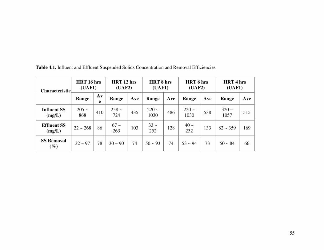
55
Table 4.1. Influent and Effluent Suspended Solids Concentration and Removal Efficiencies
HRT 16 hrs (UAF1)
HRT 12 hrs (UAF2)
HRT 8 hrs (UAF1)
HRT 6 hrs (UAF2)
HRT 4 hrs (UAF1) Characteristics
Range Ave Range Ave Range Ave Range Ave Range Ave
Influent SS (mg/L)
205 ~ 868 410 258 ~
724 435 220 ~ 1030 486 220 ~
1030 538 320 ~ 1057 515
Effluent SS (mg/L) 22 ~ 268 86 67 ~
263 103 33 ~ 252 128 40 ~
232 133 82 ~ 359 169
SS Removal (%) 32 ~ 97 78 30 ~ 90 74 50 ~ 93 74 53 ~ 94 73 50 ~ 84 66

56
Following this, anaerobic filter (UAF2) was operated at 8 hours HRT for about 288 days.
The effluent SS concentrations at 8 hours HRT were higher than that at 16 and 12 hours
HRT owing to high hydraulic loading rate at a shorter HRT. The possible reason could
be that the UAF2 was directly operated at 8 hrs HRT after the wash out incident stated
earlier.
The UAF2 was later operated at 6 hours HRT for about 198 days. The effluent SS
concentration at 6 hours HRT was higher than that at 16, 12 and 8 hours HRTs.
Subsequent shortening the HRT to 4 hours demonstrated further deterioration in the SS
removal efficiency by 7% compared with 6 hours HRT. Henz and Harremoes (1982)
explained that the cause for biomass wash out of anaerobic filters are due to gas bubbles
adhered to flocs/bed particles and caused them to rise in the reactor, eventually leading to
washout of biomass and deterioration of the effluent quality.
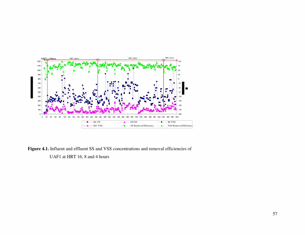
57
Figure 4.1. Influent and effluent SS and VSS concentrations and removal efficiencies of
UAF1 at HRT 16, 8 and 4 hours
0
100
200
300
400
500
600
700
800
900
1000
1100
1200
0 20 40 60 80 100 120 140 160 180 200 220 240 260 280 300 320 340 360 380 400 420 440 460 480 500 520 540 560 580 600
Day
-200
-175
-150
-125
-100
-75
-50
-25
0
25
50
75
100
Inf. SS Eff.SS Inf.VSS
Eff. VSS SS Removal Efficiency VSS Removal Efficiency
HRT = 24hrs HRT =16 hr s HRT = 8 hrs HRT = 4 hr s
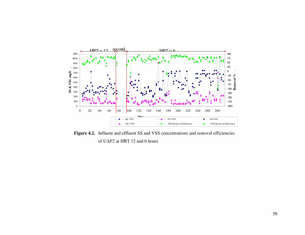
58
0
100
200
300
400
500
600
700
800
900
1000
1100
0 20 40 60 80 100 120 140 160 180 200 220 240 260 280
Day
SS &
VSS
mg/
L .
-200
-175
-150
-125
-100
-75
-50
-25
0
25
50
75
100
Rem
oval
%
.
Inf. TSS Eff.TSS Inf.VSS
Eff. VSS TSS Removal Efficiency VSS Removal Efficiency
HRT = 6 HRT = 12 second
Figure 4.2. Influent and effluent SS and VSS concentrations and removal efficiencies
of UAF2 at HRT 12 and 6 hours
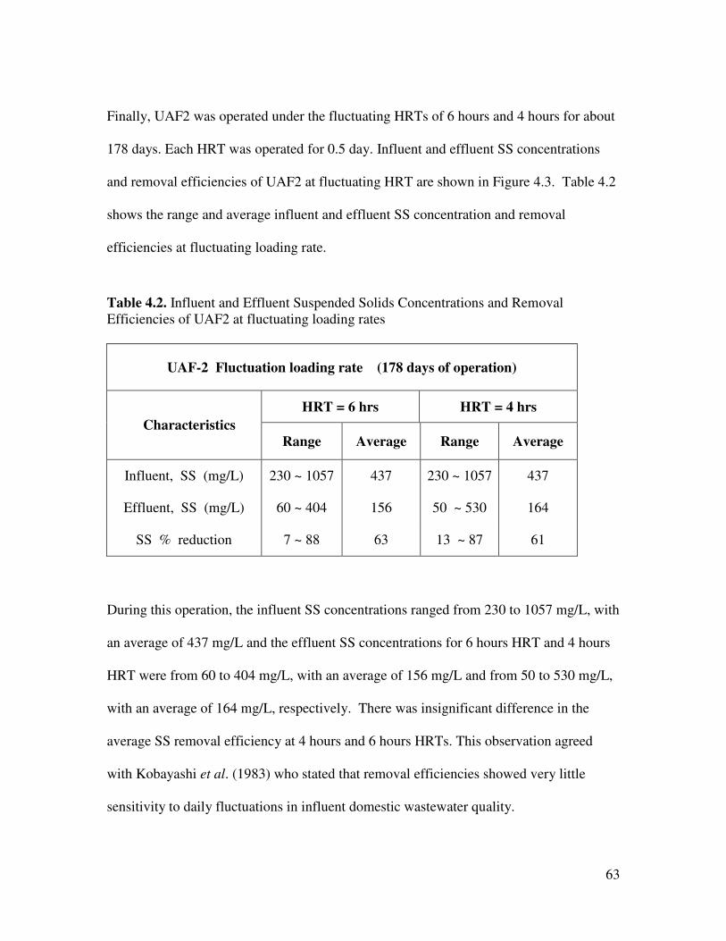
63
Finally, UAF2 was operated under the fluctuating HRTs of 6 hours and 4 hours for about
178 days. Each HRT was operated for 0.5 day. Influent and effluent SS concentrations
and removal efficiencies of UAF2 at fluctuating HRT are shown in Figure 4.3. Table 4.2
shows the range and average influent and effluent SS concentration and removal
efficiencies at fluctuating loading rate.
Table 4.2. Influent and Effluent Suspended Solids Concentrations and Removal Efficiencies of UAF2 at fluctuating loading rates
UAF-2 Fluctuation loading rate (178 days of operation)
HRT = 6 hrs HRT = 4 hrs Characteristics
Range Average Range Average
Influent, SS (mg/L) 230 ~ 1057 437 230 ~ 1057 437
Effluent, SS (mg/L) 60 ~ 404 156 50 ~ 530 164
SS % reduction 7 ~ 88 63 13 ~ 87 61
During this operation, the influent SS concentrations ranged from 230 to 1057 mg/L, with
an average of 437 mg/L and the effluent SS concentrations for 6 hours HRT and 4 hours
HRT were from 60 to 404 mg/L, with an average of 156 mg/L and from 50 to 530 mg/L,
with an average of 164 mg/L, respectively. There was insignificant difference in the
average SS removal efficiency at 4 hours and 6 hours HRTs. This observation agreed
with Kobayashi et al. (1983) who stated that removal efficiencies showed very little
sensitivity to daily fluctuations in influent domestic wastewater quality.

64
In
flue
nt a
nd E
fflu
ent T
SS
for
load
ing
fluct
uatio
n
0
200
400
600
800
1000
1200
16
1116
2126
3136
4146
5156
6166
7176
8186
9196
101
106
111
116
121
126
131
136
141
146
151
156
161
166
171
176
Day
s
TSS (mg/L)
-200
-150
-100
-50
050100
Removal Efficiency %
Inf.
TSS
Eff
.TSS
- 6
hrs
Eff
. TSS
- 4h
rsT
SS -
6 hr
s R
emov
al E
ffic
ienc
yT
SS -
4hrs
Rem
oval
Eff
icie
ncy
F
igur
e. 4
.3 In
flue
nt a
nd e
fflu
ent S
S co
ncen
trat
ions
and
rem
oval
eff
icie
ncie
s of
UA
F2 a
t
fl
uctu
atin
g H
RT
of 6
and
4 h
ours
65
From the above results, it can be concluded that shorter HRT would lead to higher SS
concentrations in the effluent and corresponding lower SS removal efficiencies. And,
based on SS removal, the optimum HRT for treatment of domestic wastewater by the
upflow anaerobic filter was found to be 6 hrs.
4.2 Volatile Suspended Solids (VSS) Removal
The influent and effluent VSS concentrations and removal efficiencies of UAF1 and
UAF2 at different HRTs are shown in the Figures 4.1 and 4.2. Table 4.3 summarizes the
range and average influent and effluent VSS concentrations and their removal
efficiencies under different HRTs.
While the influent VSS concentrations were ranged from 165 to 767 mg/L, with an
average value of 332 mg/L, the effluent VSS concentrations were ranged from 17 to 217
mg/L, with an average value of 69 mg/L at 16 hours HRT. The removal efficiencies of
VSS ranged from 26 to 97%, while the average removal efficiency was at 77%.
The effluent VSS concentration at 12 hours HRT was slightly higher than that at 16 hours
HRT. Higher effluent VSS concentration led to 4% reduction in the VSS removal
efficiency compared with that at 16 hours HRT. This was due to the high hydraulic
loading rate in a shorter HRT as stated earlier.

66
Table 4.3 Influent and Effluent Volatile Suspended Solids Concentration and Removal Efficiencies
HRT 16 hrs (UAF1)
HRT 12 hrs (UAF2)
HRT 8 hrs (UAF1)
HRT 6 hrs (UAF2)
HRT 4 hrs (UAF1)
Characteristics
Range Ave Range Ave Range Ave Range Ave Range Ave
Influent VSS (mg/L)
165 ~ 767 332 210 ~
491 329 197 ~ 793 427 197 ~
684 445 183 ~ 555 371
Effluent VSS (mg/L)
17 ~ 217 69 60 ~ 161 84 20 ~
244 110 31 ~ 224 114 62 ~ 250 128
VSS Removal (%)
26 ~ 97 77 34 ~ 87 73 50 ~ 92 73 52 ~ 93 72 39 ~ 82 64
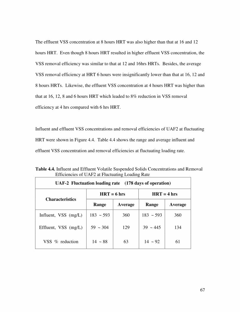
67
The effluent VSS concentration at 8 hours HRT was also higher than that at 16 and 12
hours HRT. Even though 8 hours HRT resulted in higher effluent VSS concentration, the
VSS removal efficiency was similar to that at 12 and 16hrs HRTs. Besides, the average
VSS removal efficiency at HRT 6 hours were insignificantly lower than that at 16, 12 and
8 hours HRTs. Likewise, the effluent VSS concentration at 4 hours HRT was higher than
that at 16, 12, 8 and 6 hours HRT which leaded to 8% reduction in VSS removal
efficiency at 4 hrs compared with 6 hrs HRT.
Influent and effluent VSS concentrations and removal efficiencies of UAF2 at fluctuating
HRT were shown in Figure 4.4. Table 4.4 shows the range and average influent and
effluent VSS concentration and removal efficiencies at fluctuating loading rate.
Table 4.4. Influent and Effluent Volatile Suspended Solids Concentrations and Removal Efficiencies of UAF2 at Fluctuating Loading Rate
UAF-2 Fluctuation loading rate (178 days of operation)
HRT = 6 hrs HRT = 4 hrs Characteristics
Range Average Range Average
Influent, VSS (mg/L) 183 ~ 593 360 183 ~ 593 360
Effluent, VSS (mg/L) 59 ~ 304 129 39 ~ 445 134
VSS % reduction 14 ~ 88 63 14 ~ 92 61
68
The influent VSS concentrations were ranged from 183 to 593 mg/L, with an average of
360 mg/L and the effluent VSS concentrations for 6 hours HRT and 4 hours HRT ranged
from 59 to 304 mg/L, with an average of 129 mg/L and from 39 to 445 mg/L, with an
average of 134 mg/L, respectively. Only 2 % reduction in SS removal efficiency was
observed at 4 hours compared with 6 hours of HRT.

69
Influent and Effluent VSS for loading fluctuation
0
200
400
600
800
1000
1200
1 6 11 16 21 26 31 36 41 46 51 56 61 66 71 76 81 86 91 96 101 106 111 116 121 126 131 136 141 146 151 156 161 166 171 176
Days
VS
S (m
g/L)
-200
-150
-100
-50
0
50
100
Rem
oval
Effi
cien
cy %
Inf. VSS Eff.VSS - 6 hrs Eff. VSS - 4hrs VSS - 6 hrs Removal Efficiency VSS - 4hrs Removal Efficiency Figure 4.4 Influent and effluent VSS concentrations and removal efficiencies of
UAF2 at fluctuating HRT of 6 and 4 hours
70
4.3 COD removal
The tCOD and sCOD concentrations in the influent and effluent and their removal
efficiencies in UAF1 and UAF2 under different HRTs were shown in Figures 4.5 and 4.6.
Table 4.5 summarizes the average and range of influent and effluent tCOD and sCOD
concentrations and their removal efficiencies.
The influent tCOD concentrations ranged from 343 to 803 mg/L, with an average value
of 534 mg/L at 16 hours HRT, and effluent tCOD concentrations ranged from 34 to 282
mg/L, with an average value of 128 mg/L. The influent sCOD concentrations ranged
from 45 to 211 mg/L, with an average value of 85 mg/L and the effluent sCOD
concentrations ranged from 7 to 81 mg/L, with an average value of 49 mg/L. In addition,
the removal efficiencies of tCOD and sCOD obtained were in the range from 58 to 92%,
with an average of 77% and from 11 to 92%, with an average of 41%, respectively. As
stated earlier in section 4.1, the removal efficiencies of tCOD and sCOD were below 50%
during periodical biomass washouts at 16 hours HRT. Hence, the loss of biomass during
wash out had reduced the COD removal efficiency.
At 12 hours HRT, the effluent tCOD and sCOD concentrations were higher than that at
16 hours HRT. This led to a 5% reduction in the tCOD removal efficiency and 20%
reduction in sCOD removal efficiency. The reason for the lower removal efficiency
could be due to higher organic loading rate at shorter HRT, which resulted in insufficient
time to degrade the total and soluble COD.

71
Only 2% reduction in tCOD removal efficiency at 8 hours HRT was observed when
compared with 12 hours HRT, while the sCOD removal efficiency experienced a 50%
increase.

72
Table 4.5. Influent and Effluent tCOD and sCOD Concentrations and Removal Efficiencies
HRT 16 hrs (UAF1)
HRT 12 hrs (UAF2)
HRT 8 hrs (UAF1)
HRT 6 hrs (UAF2)
HRT 4 hrs (UAF1)
Characteristics
Range Ave Range Ave Range Ave Range Av
e Range Ave
Influent tCOD (mg/L)
343 ~ 803 534 391 ~
707 521
194 ~ 1134 579 311 ~
1134 609
298 ~ 783
462
Effluent tCOD (mg/L)
34 ~ 282 128 53 ~ 336
140
41 ~ 428 168 45 ~ 897 17
8 98 ~ 313
181
tCOD Removal (%)
58 ~ 92 77 29 ~ 88 72 44 ~ 93 70 36 ~ 93 68 50 ~ 73 60
Influent sCOD (mg/L)
45 ~ 211 85 37 ~ 211 90 32 ~
191 91 43 ~ 191 93 15 ~ 150 85
Effluent sCOD (mg/L)
7 ~ 81 49 35 ~ 116 73 9 ~ 77 43 8 ~ 138 55 11 ~ 97 49
sCOD Removal (%)
11 ~ 92 41 4 ~ 62 21 21 ~ 89 50 10 ~ 89 45 13 ~ 64 41

73
0
100
200
300
400
500
600
700
800
900
1000
1100
1200
0 20 40 60 80 100 120 140 160 180 200 220 240 260 280 300 320 340 360 380 400 420 440 460 480 500 520 540 560 580 600
Day
tCO
D &
sC
OD
(mg/
L)
-200
-175
-150
-125
-100
-75
-50
-25
0
25
50
75
100
Rem
oval
%
Inf.tCOD Eff.tCOD Inf. sCOD
Eff.sCOD tCOD Removal Efficiency sCOD Removal Efficiency
HRT = HRT = 16 hrs HRT = 8 hrs HRT = 4 hrs
Figure 4.5 Influent and effluent tCOD and sCOD concentrations and removal efficiencies of UAF1
at HRT 16, 8 and 4 hours

74
0
100
200
300
400
500
600
700
800
900
1000
010
2030
4050
6070
8090
100
110
120
130
140
150
160
170
180
190
200
210
220
230
240
250
260
270
280
290
Day
-200
-175
-150
-125
-100
-75
-50
-25
0255075100
Removal %
Inf.
tCO
DE
ff.t
CO
DIn
f. s
CO
D
Eff
.sC
OD
tCO
D R
emo
val E
ffic
ienc
ysC
OD
Rem
ova
l Eff
icie
ncy
HR
T=
6hrs
HR
T =
12 h
rsse
cond
see
ding
ig
ure
4.6
Infl
uent
and
eff
luen
t tC
OD
and
sC
OD
con
cent
ratio
ns a
nd re
mov
al e
ffic
ienc
ies
of
UA
F2 a
t HR
T 1
2 an
d 6
hour
s

75
The effluent tCOD and sCOD concentrations at 6 hours HRT were slightly higher than
that at 16, 12 and 8 hours HRT. The reductions in removal efficiencies of tCOD and
sCOD were 2 % and 5%, respectively. A significant amount of reduction in tCOD
removal efficiency (8%) was observed at 4 hours HRT compared with 6 hours HRT,
while only 4% reduction in sCOD was noted.
Nebot et al. (1995) pointed out that the characterization of performance of the anaerobic
filter versus organic load added is important. Several studies have been carried out to
study the influence of the organic load shocks in the anaerobic filter. Consequently,
Panswad and Komolmethee, (1997) mentioned that this shock can be produced by both
the applied volumetric flow rate and the increase in the added organic load – these are
called hydraulic shock or organic shock, respectively. The influent and effluent tCOD
and sCOD concentrations and removal efficiencies of UAF2 at fluctuating HRT are
shown in Figures 4.7 and 4.8, respectively. Table 4.6 shows the range and average of
influent and effluent tCOD and sCOD concentrations and removal efficiencies at
fluctuating loading rate.
The influent tCOD concentrations were in the range of 343 to 956 mg/L, with an average
value of 579 mg/L and the effluent tCOD concentrations for 6 hours HRT and 4 hours
HRT were ranged from 59 to 415 mg/L, with an average of 194 mg/L and 95 to 315
mg/L, with an average of 219 mg/L, respectively.

76
Table 4.6. Influent and Effluent tCOD and sCOD Concentrations and Removal Efficiencies of UAF2 at Fluctuating Loading Rate
UAF-2 Fluctuation loading rate (178 days of operation)
HRT = 6 hrs HRT = 4 hrs Characteristics
Range Average Range Average
Influent, tCOD (mg/L) 343 ~ 956 579 343 ~ 956 579
Effluent, tCOD (mg/L) 59 ~ 415 194 95 ~ 315 219
tCOD % reduction 20 ~ 89 65 30 ~ 86 59
Influent, sCOD (mg/L) 14 ~ 143 87 14 ~ 143 87
Effluent, sCOD (mg/L) 11 ~ 96 57 9 ~ 109 60
sCOD % reduction 15 ~ 81 33 10 ~ 77 30
The influent sCOD concentrations were in the range of 14 to 143 mg/L, with an average
value of 87 mg/L and the effluent sCOD concentrations for 6 hours HRT and 4 hours
HRT were ranged from 11 to 96 mg/L, with an average of 57 mg/L and 9 to 109 mg/L,
with an average of 60 mg/L, respectively.
The removal efficiencies of tCOD for 6 hours HRT and 4 hours HRT were from 20 to
89%, with an average of 65% and from 30 to 86%, with an average of 59%, respectively.
While the removal efficiencies of sCOD for 6 hours HRT and 4 hours HRT were ranged
from 15 to 81%, with an average of 33% and from 10 to 77%, with an average of 30%,
respectively. The observed COD removal results show that anaerobic filter performed
similarly for 6 hours and 4 hours fluctuating HRT. This obsercvation agreeded with
Herbert et al. (1994) who reported that the percentage of COD removal from wastewater
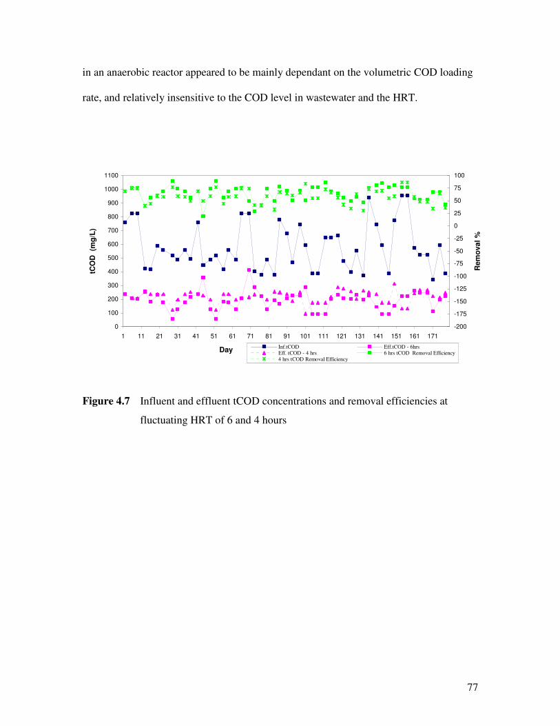
77
in an anaerobic reactor appeared to be mainly dependant on the volumetric COD loading
rate, and relatively insensitive to the COD level in wastewater and the HRT.
0
100
200
300
400
500
600
700
800
900
1000
1100
1 11 21 31 41 51 61 71 81 91 101 111 121 131 141 151 161 171
Day
tCO
D (
mg/
L)
-200
-175
-150
-125
-100
-75
-50
-25
0
25
50
75
100
Rem
oval
%
Inf.tCOD Eff.tCOD - 6hrsEff. tCOD - 4 hrs 6 hrs tCOD Removal Efficiency4 hrs tCOD Removal Efficiency
Figure 4.7 Influent and effluent tCOD concentrations and removal efficiencies at
fluctuating HRT of 6 and 4 hours

78
0
20
40
60
80
100
120
140
160
1 11 21 31 41 51 61 71 81 91 101 111 121 131 141 151 161 171
Day
sCO
D (
mg/
L)
-200
-175
-150
-125
-100
-75
-50
-25
0
25
50
75
100
Rem
oval
%
Inf.sCOD Eff.sCOD - 6hrsEff. sCOD - 4 hrs 6 hrs sCOD Removal Efficiency4 hrs sCOD Removal Efficiency
Figure 4.8 Influent and effluent sCOD concentrations and removal efficiencies at of
UAF2 fluctuating HRT of 6 and 4 hours

79
4.4 BOD5 Removal
The tBOD and sBOD concentrations of influent and effluent and their removal
efficiencies of UAF1 and UAF2 under different HRTs are shown in Figures 4.9 and 4.10,
respectively. The average and range of influent and effluent tBOD and sBOD
concentrations and their removal efficiencies are summarized in Table 4.7.
At 16 hours HRT, the influent tBOD5 concentrations were in the range of 138 to 436
mg/L, with an average value of 226 mg/L and the effluent tBOD5 concentrations ranged
from 10 to 85 mg/L, with an average value of 44 mg/L. The influent sBOD5
concentrations ranged from 9 to 43 mg/L, with an average value of 24 mg/L and the
effluent sBOD5 concentrations ranged from 2 to 30 mg/L, with an average value of 13
mg/L. The removal efficiencies of tBOD5 and sBOD5 ranged from 59 to 94%, with an
average of 79% and from 8 to 75%, with an average of 53%, respectively.
At 12 hours HRT, the removal efficiencies of tBOD5 and sBOD5 ranged from 48 to 91%
with an average of 67% and from 25 to 41% with an average of 33%, respectively. There
were 12% reduction in tBOD removal efficiency and 20% reduction in sBOD removal
efficiency were observed at 12hours HRT when compared with 16 hours HRT, which
was comparable with Kobayashi et al. (1983) results (BOD removal 79%, COD removal
73%).

80
0
50
100
150
200
250
300
350
400
450
500
0 20 40 60 80 100 120 140 160 180 200 220 240 260 280 300 320 340 360 380 400 420 440 460 480 500 520 540 560 580 600
Day
-200
-175
-150
-125
-100
-75
-50
-25
0
25
50
75
100
Inf.tBOD Eff.tBODInf. sBOD Eff. sBODtBODRemoval Efficiency sBOD Removal Efficiency
HRT = 24 HRT = 16 hr s HRT = 8 hr s HRT = 4 hr s
Figure 4.9. Influent and effluent tBOD5 and sBOD5 concentrations and removal efficiencies of
UAF1 at HRT 16, 8 and 4 hours
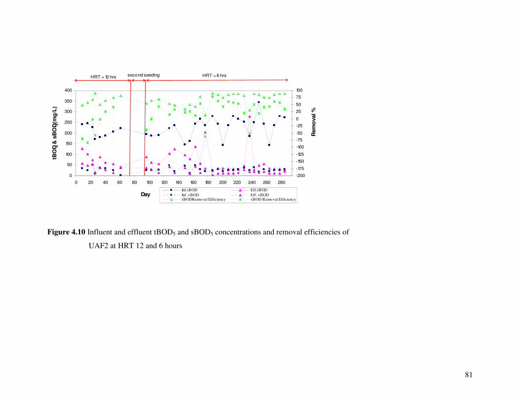
81
0
50
100
150
200
250
300
350
400
0 20 40 60 80 100 120 140 160 180 200 220 240 260 280
Day
tBO
D 5 &
sB
OD 5
(mg
/L)
-200
-175
-150
-125
-100
-75
-50
-25
0
25
50
75
100
Rem
ova
l %
Inf.tBOD Eff.tBODInf. sBOD Eff. sBODtBODRemoval Efficiency sBOD Removal Efficiency
HRT = 6 hrssecond seedingHRT = 12 hrs
Figure 4.10 Influent and effluent tBOD5 and sBOD5 concentrations and removal efficiencies of
UAF2 at HRT 12 and 6 hours

82
Table 4.7 Influent and Effluent tBOD and sBOD Concentrations and Removal Efficiencies
HRT 16 hrs
(UAF1) HRT 12 hrs
(UAF2) HRT 8 hrs
(UAF1) HRT 6 hrs
(UAF2) HRT 4 hrs
(UAF1) Characteristics
Range Ave
Range Ave Range Ave Range Ave Range Ave
Influent tBOD5 (mg/L)
138 ~ 436
226
172 ~ 245 210 141 ~
346 233 144 ~ 346 230 111 ~
311 227
Effluent tBOD5 (mg/L)
10 ~ 85 44 16 ~ 127 71 29 ~
142 54 24 ~ 279 71 32 ~ 115 60
tBOD5 Removal (%)
59 ~ 94 79 48 ~ 91 67 54 ~ 89 76 33 ~ 92 75 33 ~ 87 70
Influent sBOD5 (mg/L)
9 ~ 43 24 3 ~ 52 27 11 ~ 49 28 11 ~ 49 29 17 ~ 47 29
Effluent sBOD5 (mg/L)
2 ~ 30 13 13 ~ 58 36 8 ~ 22 13 5 ~ 43 20 10 ~ 25 14
sBOD5 Removal (%)
8 ~ 75 53 25 ~ 41 33 17 ~ 71 49 12 ~ 80 42 18 ~ 77 47
83
Likewise, while comparing removal efficiencies of tBOD and sBOD at 8 and 12 hours
HRTs, there were significant reductions of 9 and 16 % in tBOD and sBOD at 8 hours
HRT. There was no significant change in tBOD removal efficiency at 6 hours HRT
compared with 8 hours HRT, however, a 7 % reduction in sBOD removal efficiency was
observed.
Approximately, 5% reduction in removal efficiency of tBOD was observed at 4 hours
HRT compared with 6 hours HRT. However, the sBOD removal efficiency experienced
an increase of 5% at 4 hours HRT.
The influent and effluent tBOD and sBOD concentrations and removal efficiencies of
UAF2 at fluctuating HRT are shown in Figures 4.11 and 4.12, respectively. Table 4.8
shows the range and average of influent and effluent tBOD and sBOD concentrations and
removal efficiencies at fluctuating loading rate.
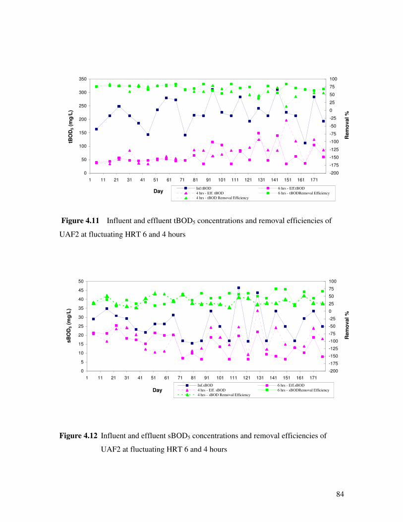
84
0
50
100
150
200
250
300
350
1 11 21 31 41 51 61 71 81 91 101 111 121 131 141 151 161 171
Day
tBO
D5
(mg/
L)
-200
-175
-150
-125
-100
-75
-50
-25
0
25
50
75
100
Rem
oval
%
Inf.tBOD 6 hrs - Eff.tBOD4 hrs - Eff. tBOD 6 hrs - tBODRemoval Efficiency4 hrs - tBOD Removal Efficiency
Figure 4.11 Influent and effluent tBOD5 concentrations and removal efficiencies of
UAF2 at fluctuating HRT 6 and 4 hours
0
5
10
15
20
25
30
35
40
45
50
1 11 21 31 41 51 61 71 81 91 101 111 121 131 141 151 161 171
Day
sBO
D5
(mg/
L)
-200
-175
-150
-125
-100
-75
-50
-25
0
25
50
75
100
Rem
oval
%
Inf.sBOD 6 hrs - Eff.sBOD4 hrs - Eff. sBOD 6 hrs - sBODRemoval Efficiency4 hrs - sBOD Removal Efficiency
Figure 4.12 Influent and effluent sBOD5 concentrations and removal efficiencies of
UAF2 at fluctuating HRT 6 and 4 hours
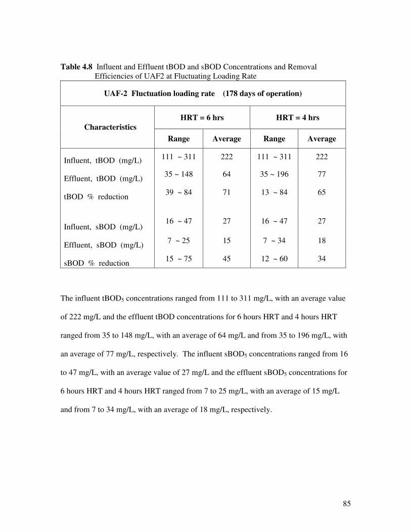
85
Table 4.8 Influent and Effluent tBOD and sBOD Concentrations and Removal Efficiencies of UAF2 at Fluctuating Loading Rate
UAF-2 Fluctuation loading rate (178 days of operation)
HRT = 6 hrs HRT = 4 hrs Characteristics
Range Average Range Average
Influent, tBOD (mg/L) 111 ~ 311 222 111 ~ 311 222
Effluent, tBOD (mg/L) 35 ~ 148 64 35 ~ 196 77
tBOD % reduction 39 ~ 84 71 13 ~ 84 65
Influent, sBOD (mg/L) 16 ~ 47 27 16 ~ 47 27
Effluent, sBOD (mg/L) 7 ~ 25 15 7 ~ 34 18
sBOD % reduction 15 ~ 75 45 12 ~ 60 34
The influent tBOD5 concentrations ranged from 111 to 311 mg/L, with an average value
of 222 mg/L and the effluent tBOD concentrations for 6 hours HRT and 4 hours HRT
ranged from 35 to 148 mg/L, with an average of 64 mg/L and from 35 to 196 mg/L, with
an average of 77 mg/L, respectively. The influent sBOD5 concentrations ranged from 16
to 47 mg/L, with an average value of 27 mg/L and the effluent sBOD5 concentrations for
6 hours HRT and 4 hours HRT ranged from 7 to 25 mg/L, with an average of 15 mg/L
and from 7 to 34 mg/L, with an average of 18 mg/L, respectively.

86
The removal efficiencies of tBOD5 for 6 hours HRT and 4 hours HRT ranged from 39 to
84% with an average of 71% and from 13 to 84% with an average of 65%, respectively.
The removal efficiencies of sBOD5 for 6 hours HRT and 4 hours HRT ranged from 18 to
75% with an average of 45% and from 12 to 60% with an average of 34%, respectively.
The results show that the anaerobic filter performance at 6 hours and 4 hours fluctuating
HRT in terms of tBOD5 and COD removal did not differ significantly. It could be
concluded that anaerobic filter performed similarly at 6 hours and 4 hours fluctuating
HRT in terms of the solids, COD and BOD5 removal. In addition, this study
demonstrated that the anaerobic filter was able to withstand shock loadings and perform
well with the help of the attached biofilm.
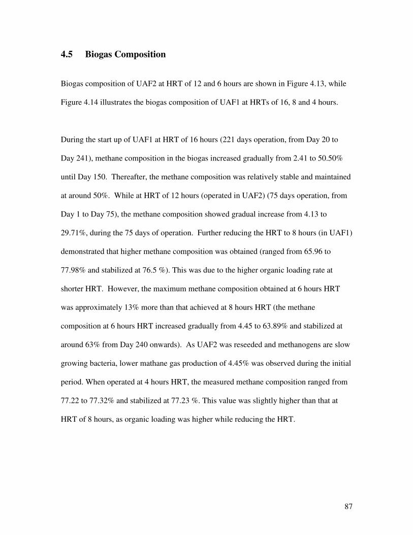
87
4.5 Biogas Composition
Biogas composition of UAF2 at HRT of 12 and 6 hours are shown in Figure 4.13, while
Figure 4.14 illustrates the biogas composition of UAF1 at HRTs of 16, 8 and 4 hours.
During the start up of UAF1 at HRT of 16 hours (221 days operation, from Day 20 to
Day 241), methane composition in the biogas increased gradually from 2.41 to 50.50%
until Day 150. Thereafter, the methane composition was relatively stable and maintained
at around 50%. While at HRT of 12 hours (operated in UAF2) (75 days operation, from
Day 1 to Day 75), the methane composition showed gradual increase from 4.13 to
29.71%, during the 75 days of operation. Further reducing the HRT to 8 hours (in UAF1)
demonstrated that higher methane composition was obtained (ranged from 65.96 to
77.98% and stabilized at 76.5 %). This was due to the higher organic loading rate at
shorter HRT. However, the maximum methane composition obtained at 6 hours HRT
was approximately 13% more than that achieved at 8 hours HRT (the methane
composition at 6 hours HRT increased gradually from 4.45 to 63.89% and stabilized at
around 63% from Day 240 onwards). As UAF2 was reseeded and methanogens are slow
growing bacteria, lower mathane gas production of 4.45% was observed during the initial
period. When operated at 4 hours HRT, the measured methane composition ranged from
77.22 to 77.32% and stabilized at 77.23 %. This value was slightly higher than that at
HRT of 8 hours, as organic loading was higher while reducing the HRT.
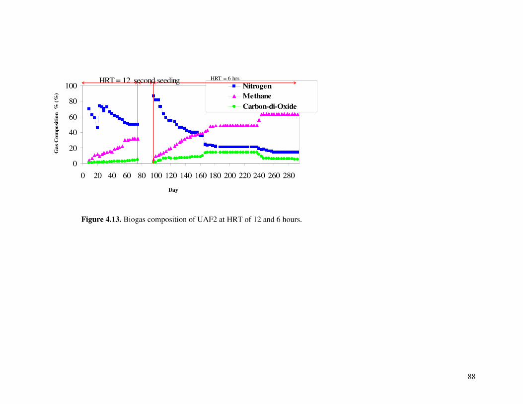
88
0
20
40
60
80
100
0 20 40 60 80 100 120 140 160 180 200 220 240 260 280
Day
Gas
Com
posit
ion
% (%
)
NitrogenMethaneCarbon-di-Oxide
HRT = 6 hrsHRT = 12 second seeding
Figure 4.13. Biogas composition of UAF2 at HRT of 12 and 6 hours.

89
0
10
20
30
40
50
60
70
80
90
100
0 20 40 60 80 100 120 140 160 180 20
0
22
0
24
0
26
0
28
0
30
0
32
0
34
0
36
0
38
0
40
0
42
0
44
0
46
0
48
0
50
0
52
0
54
0
56
0
58
0
60
0
Day
NitrogenMethaneCarbon-di-oxide
HRT = HRT = 24 hrs
HRT = 8 HRT = 4
Figure 4.14. Biogas composition of UAF1 at HRT of 16, 8 and 4 hours.

90
4.6 Biogas Production
Biogas production of UAF1 at HRTs of 16, 8 and 4 hours and UAF2 at HRTs of 12 and 6
hours are shown in Figures 4.15 and 4.16, respectively.
During the UAF1 start up period at 16 hours HRT, biogas production increased gradually
from 0.09 to 0.97 L/d. On Day 139, biogas leakage near effluent port was noted and was
later replaced with a T-junction setup. After the retrofitting, an increase in the biogas
production volume was observed. From Day 150, the biogas production was rather stable
at around 0.75 L/d.
Similarly, the biogas production also showed gradual increase during the UAF2 start up
period at 12 hours HRT within the 75 days operation. Higher biogas production was
observed at 8 hours HRT in UAF1 due to the higher organic loading rate. The biogas
production ranged from 0.97 to 2.62 L/d and stabilized at around 2 L/d. Hence,
shortening the HRT by half had contributed to an increase in biogas production by almost
2.6 times. However, due to reseeding of UAF2 at 6 hours HRT, the biogas production
increased gradually from 0.88 to only up to 1.46 L/d and eventually only stabilized at
around 1.42 L/d from day 115. Further shortening the HRT to 4 hours gave rise to biogas
production ranged from 2.12 to 2.63 L/d and stabilized around 2.19 L/d. The biogas
production at 4 hours HRT was only 9.5% more than that at 8 hours HRT.
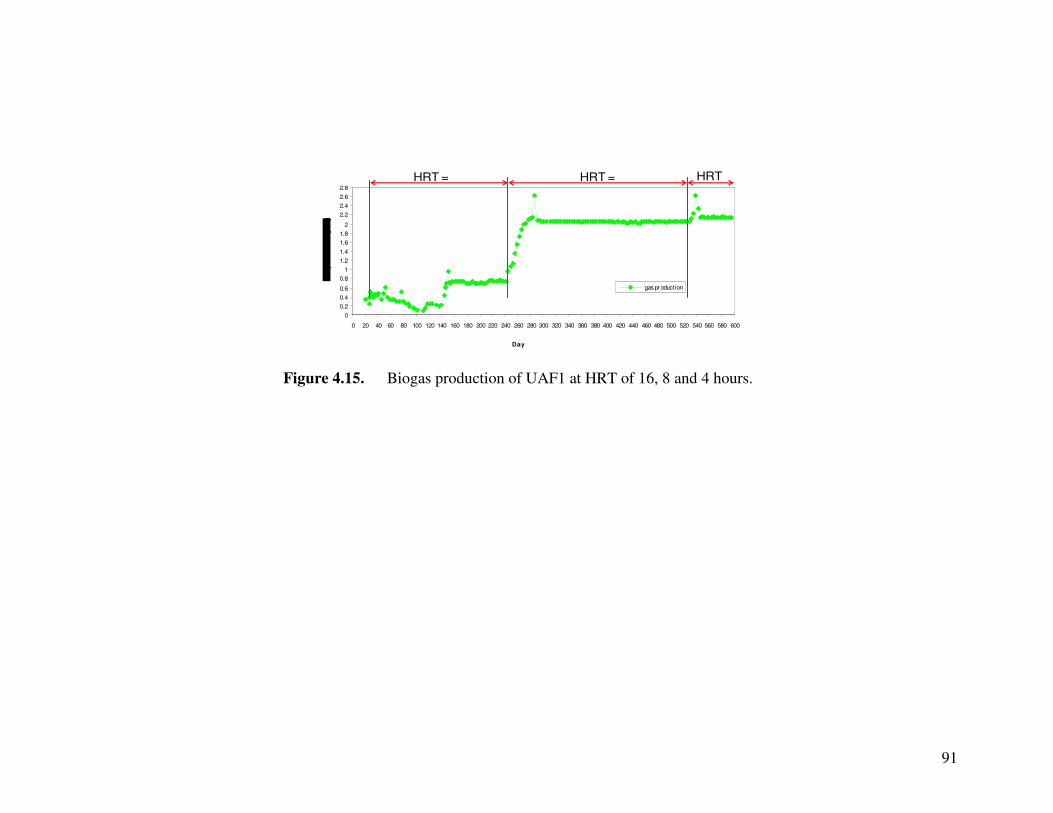
91
00.20.40.6
0.81
1.21.41.61.8
2
2.22.42.62.8
0 20 40 60 80 100 120 140 160 180 200 220 240 260 280 300 320 340 360 380 400 420 440 460 480 500 520 540 560 580 600
Day
gas pr oduction
HRT = HRT = HRT
Figure 4.15. Biogas production of UAF1 at HRT of 16, 8 and 4 hours.

92
0.0
0.2
0.4
0.6
0.8
1.0
1.2
1.4
1.6
020
4060
8010
012
014
016
018
020
022
024
026
028
0
Day
Gas production (L/d)
Gas
pro
duct
ion
HR
T =
6 hr
sse
cond
se
edin
gH
RT
= 12
hr
s
Figu
re 4
.16.
Bio
gas
prod
uctio
n of
UA
F2 a
t HR
T o
f 12
and
6 ho
urs.

93
4.7. Suspended Biomass (MLSS and MLVSS)
The suspended biomass concentration of anaerobic filter was measured in terms of MLSS
and MLVSS. The suspended biomass sample was collected from the sampling port
located 0.37 m from the top of the reactor. The suspended biomass concentrations of
UAF2 at HRT of 12 and 6 hours and UAF1 at HRT of 16, 8 and 4 hours are shown in
Figures 4.17 and 4.18, respectively.
During the UAF1 start up at HRT of 16 hours, the MLSS and MLVSS concentrations
ranged from 2411 to 8517 mg/L with an average of 5543 mg/L and from 2000 to 6167
mg/L with an average of 3794 mg/L, respectively. The MLSS and MLVSS
concentrations during the UAF2 start up at HRT of 12 hours were significantly higher
which ranged from 5360 to 13073 mg/L with an average value of 7841 mg/L and from
3673 to 8209 mg/L with an average value of 5340 mg/L, respectively. Consequently,
during 8 hrs of HRT, the MLSS and MLVSS concentrations were observed to range from
3567 to 13,856 mg/L and from 2600 to 9856 mg/L, respectively. And the average MLSS
and MLVSS concentrations were 6374 and 5022 mg/L at 8 hours of HRT. While
comparing MLSS and MLVSS concentrations of 16 and 8 hours HRTs, an increase in
concentrations of 13% and 24%, respectively, was observed due to higher organic
loading at 8 hours HRT than 16 hours. The reasons for this could be higher hydraulic
loading rate would have sloughed off the attached biofilm and higher organic loading
would have increased the suspended biomass concentration in UAF1.

94
Moreover, during 6 hrs of HRT, the MLSS and MLVSS ranged from 4067 to 17,722
mg/L and from 3,467 to 12,644 mg/L, respectively. And the average MLSS and MLVSS
concentrations were 10,110 and 8058 mg/L at 6 hrs of HRT. Finally, during 4 hrs of HRT,
the MLSS and MLVSS ranged from 4267 to 7656 mg/L and from 2711 to 7111 mg/L,
respectively. And the average MLSS and MLVSS concentrations were 6265 and 4758
mg/L at 4 hrs of HRT.
The general trend shows that reducing the HRT resulted in increased MLSS and MLVSS
in the anaerobic filter. Shortening the HRT had increased the loading rate which in turn
provided more organics and nutrient that stimulated higher growth rate.
0
2000
4000
6000
8000
10000
12000
14000
16000
18000
20000
0 20 40 60 80 100 120 140 160 180 200 220 240 260 280
Day
MLS
S &
MLV
SS
(mg/
L) MLSS (mg/L)
MLVSS (mg/L)
HRT = HRT = 6 second seeding
Figure 4.17. MLSS and MLVSS concentrations of the suspended biomass of UAF2
at HRT of 12 and 6 hours.

95
0
2000
4000
6000
8000
10000
12000
14000
16000
0 20 40 60 80 100 120 140 160 180 200 220 240 260 280 300 320 340 360 380 400 420 440 460 480 500 520 540 560 580 600
D a y
MLSSMLVSS
HRT = HRT = 16 hrs HRT = 8 hrs HRT = 4 hrs
Figure 4.18. MLSS and MLVSS concentrations of the suspended biomass of
UAF1 at HRT of 16, 8 and 4 hours.

96
4.8 Attached Biomass (MLSS and MLVSS)
Henze and Harremoes (1982) indicated that there is a wide variation in the attached
biomass content in the upflow anaerobic filters. In addition, they observed that 80% of
the biomass in an anaerobic filter was attached and the rest was suspended.
Miyahara et al. (1995) found that the number of suspended acidogenic bacteria in an AF
reactor was higher than that of bacteria attached to the media. On the other hand, the
number of attached methanogenic bacteria was higher than the number of suspended
methtanogenic bacteria.
The attached biomass concentration in the UAF2 reactor was measured at Day 200 by
taking two samples of media. After washing with tap water, the biomass concentration in
the washing water from each sample was measured. Based on these data, the MLSS and
MLVSS of attached biomass concentrations in the UAF2 reactor were estimated as
18,000 mg/L and 14,200 mg/L at 12 hours HRT. This observation agreeded with
Emitwalli et al. (2002b) who revealed that MLVSS concentration of 15,100 mg/L.
Subsequently, the attached biomass contains MLSS of 12,654 mg/L and MLVSS of
10,743 mg/L at 6 hrs of HRT. While comparing 12 and 6 hrs of HRT, it was observed
that there was a reduction in attached biomass concentration. Hydraulic effect of higher
hydraulic load sloughed off of the attached biomass.

97
4.9 Mass balance (carbon balance) of UAF1 at HRT 8 hours
The following experimental data of steady conditions are used for the calculation and
estimation.
Flowrate Q = 61.5 L/d
Avg. CH4 % = 76.5%
Avg. biogas production = 2.0 L/d
Avg. tCODinf = 579 mg/L
Avg. tCODeff = 168 mg/L
Calculation of CH4 dissolved in the liquid (effluent)
CH4 solubility at 1 atm ~ 20 mg/L
CH4 partial pressure = 0.765 atm (as UASB avg. CH4 % = 76.5%)
Dissolved CH4 = 0.765 x 20 mg/L = 15.3 mg/L = 0.9563 m mol/L
Flowrate Q = 61.5 L/d
Dissolved CH4 in the effluent (loss) = 61.5 L/d x 0.9563 m mol/L = 58.81 m mol/d =
0.05881 mol/d
Avg. biogas production = 2.0 L/d (biogas collected)
CH4 production = 2.0 L/d x 76.5% = 1.53 L/d (CH4 collected at 1 atm & 300C)

98
Based on PV = nRT
P1V1/T1 = P0V0/T0
At standard condition: P0 = 1 atm, T0 = 00C = 273 K, 1 mol gas = 22.4 L
P1 = 1 atm, V1 = 1.53 L/d, T1 = 300C = 303 K
V0 = 1.3785 L/d (at standard condition) = 0.06154 mol/d
The amount of CH4 collected n = 0.06154 mol/d
Loss rate of CH4 dissolved in the liquid (effluent)
= (0.05881mol/d) / ((0.06154 mol/d) + (0.05881 mol/d))
= 48.87%
Mass balance calculation
Total CODin = tCODinf x Flowrate Q = 579 mg/L x 61.5 L/d = 35608.5 mg/d = 35.61 g/d
There is no sludge wasting in the AnF operation, so waste sludge-COD = 0.
The loss due to sampling is ignored.
At steady conditions, assume no reactor biomass change.
If the COD loss as CO2 is not considered, then
Total CODout = (tCODeff x Flowrate Q) + CH4-COD
tCODeff x Flowrate Q = 168 mg/L x 61.5 L/d = 10332 mg/d = 10.332 g/d
99
Based on CH4 + 2O2 CO2 + 2 H2O
CH4 collected = 1.3785 L/d = 0.06154 mol/d
CH4-COD collected = 2 x 0.06154 mol/d = 0.1231 mol/d = (0.1231 x 32) g/d = 3.939 g/d
Because the loss rate of CH4 dissolved in the liquid (effluent) = 48.87%, then
Total CH4-COD = 7.704 g/d
Total CODout = 10.332 g/d + 7.704 g/d = 18.036 g/d
Recovery rate = (18.036 g/d) / (35.61 g/d) = 51%
4.10 Operational Problems:
Gas bubbles entrapped in filters may cause channeling and short-circuiting in the reactor
(Henz and Harremoes, 1982). In full scale studies, filter clogging has been reported after 18
months of continuous operation (Subbiah, 1997). Kobayashi et al (1983) operated two
larger scale filters 0.6 m in diameter by 2.6m high) and experienced no clogging problems
in three years of operation. Similarly, operational problems like channeling, short-
circuiting and clogging were not observed during the entire period of this research study.
However, additional work is still required to evaluate clogging problems.
100
5��Conclusion & Recommendations
5.1 Conclusion
It has been shown that an anaerobic filter operating at high and low loading rate can
successfully treat domestic wastewater at temperature of 300C. The results show that the
anaerobic filter performance at different HRTs in terms of tBOD5 and COD removal did
not differ significantly. It could be concluded that anaerobic filter performed similarly at
6 hours and 4 hours fluctuating HRT in terms of the solids, COD and BOD5 removal. In
addition, this study demonstrated that the anaerobic filter was able to withstand shock
loadings and perform well with the help of the attached biofilm. Moreover, effluent
quality did not achieve secondary effluent quality standards but came very close.
Anaerobic process could also be followed by aerobic processes for effluent polishing to
utilize the benefits of both processes. Series reactors of anaerobic-aerobic processes have
been feasible for treating municipal wastewaters in warmer climates resulting in lower
energy requirements and less sludge production. It could be concluded that the anaerobic
filter is a promising candidate for treatment of low strength wastewaters and that post
treatment for sulfides and ammonia may be necessary.

101
5.2 Recommendations
� Start-up of anaerobic reactors is more time consuming and is subjected to
disturbances more than that of aerobic reactors. Many researchers have reported
long start-up periods of 2-3 months to 1 year (or even more) for the anaerobic
reactors. The start-up of the anaerobic process is still considered as a major area
of research. Considerable efforts have been made to study the granulation process
but the mechanism involved in the formation of granulation sludge is still
unknown. Therefore, it is recommended that further research have to be done on
start-up of anaerobic process and granule formation of sludge.
� Study on UAF with separation of phases can be carried out. Separation of phases
enables selection of optimal conditions for both processes –
acidogenesis/fermentation and acetogenesis/methanogenesis. As fermentation (pH
5.2 – 5.9) proceeds at a much greater speed than acetogenesis/methanogenesis
(pH 7.3 – 7.6), the former is carried out in acidic conditions in a separate reactor.
So, it is recommended that further study have to be done on UAF with phase
separation.
� It is well known that the operational state of high-rate anaerobic system can
change within a few hours in response to a process disturbance. On the other hand,
because of the special hydrodynamics in the reactors, the response of the

102
system output is deferred corresponding to an input variation. In order to provide
prompt corrective response, which is required in case of organic overload shocks
or toxic events, techniques that provide responses are needed to avoid the
significant process deterioration and failure. In order to be effective for on-line
control, a model can be developed to make predictions of the system response to
the variations of organic, hydraulic and alkalinity loading rates. Based on the
observed results a Monod-type of kinetic model can be developed to predict the
performance of the reactor and methane content in produced biogas.
� The use of an adequate recycling ratio is a key factor for the optimization of the
anaerobic treatment of these wastewaters, since it increases mass transfer rates,
minimizes dead zones and allows development of more equilibrated consortia of
bacteria, belonging to different trophic groups, along the reactor. it is
recommended that further study have to be done on UAF with phase separation.
Therefore, it is recommended that further research have to be done on UAF with
recycling ratio.
6. REFERENCES:

103
Adrianus, C.V.H. and G. Lettinga. Anaerobic Sewage Treatment: A Practical Guide for
Regions with a Hot Climate. pp. 179-264, England: John Wiley & Sons. 1994.
Alves, M.M., J.A. Mota, R.M. Alvares Pereira, M.A. Pereira. and M. Mota. Effect of
Lipids and Oleic Acid on Biomass Development in Anaerobic Fixed-bed Reactors, Part 1:
Biofilm Growth and Activity, Water Research, Vol 35, Iss 1, pp. 255-263. 2001.
Athanasopoulos, N., J. Kouinis. and A. Papadimitriou. A Note on Anaerobic Treatment
of Currant-finishing Wastewater in Down-flow Anaerobic Filters and The Effect of
Media Design on Their Performance, Biological Wastes, Vol 32, pp. 91-97. 1990.
Bello-Mendoza, R. and M.F. Castillo-Rivera. Start-up of An Anaerobic Hybrid
(UASB/Filter) Reactor Treating Wastewater from a Coffee Processing Plant, Anaerobe,
Vol 4, pp. 219-225. 1998.
Blonskaja, V., A. Menert. and R. Vilu. Use of Two Stage Anaerobic Treatment for
Distillery Waste, Advances in Environmental Research, Vol 7, pp. 671-678. 2003.
Bodik, I., B. Herdova. and K. Kratochvil. The Application of Anaerobic Filter for
Municipal Wastewater Treatment, Chemical Papers, Vol 54, Iss 3, pp. 159-164. 2000.
104
Bodik, I., B. Herdova. and M. Drtil. The Use of Upflow Anaerobic Filter and AnSBR for
Wastewater Treatment at Ambient Temperature, Water Research, Vol 36, Iss 4, pp. 1084-
1088. 2002.
Bodik, I., K. Kratochvil, E. Gasparikova. and M. Hutnan. Nitrogen Removal in An
Anaerobic Baffled Filter Reactor With Aerobic Post-treatment, Bioresource Technology,
Vol 86, pp. 79-84. 2003.
Boero, V.J., A.R. Bowers. and W.W.Jr. Eckenfelder. Molecular Weight Distribution of
Soluble Microbial Products in Biological Systems, Water Science Technology, Vol 34,
Iss 5-6, pp. 241-248. 1996.
Bruce, E.L. and A.W. Gretchen. Molecular Size Distribution of Dissolved Organic
Matter in Wastewater Transformed by Treatment in a Full-scale Trickling Filter, Water
Environment Research, Vol 72, Iss 3, pp. 277-281. 2000.
Buyukkamaci, N. and A. Filibeli. Volatile Fatty Acid Formation in An Anaerobic Hybrid
Reactor, Process Biochemistry, Vol 39, pp. 1491-1494. 2004.
Cakir, F.Y. and M.K. Stenstrom. A Dynamic Model for Anaerobic Filter, Journal of
Environmental Science and Health, Vol A38, Iss 10, pp. 2069-2076. 2003.

105
Callado, N.H. and E. Foresti. Removal of Organic Carbon, Nitrogen and Phosphorous in
Sequential Batch Reactors Integrating the Aerobic/Anaerobic Processes, Water Science
Technology, Vol 44, Iss 4, pp. 263-270. 2001.
Chernicharo, C.A.L. and R.M.G. Machado. Feasibility of The UASB/AF System for
Domestic Sewage Treatment in Developing Countries, Water Science Technology, Vol
38, Iss 8-9, pp. 325-332. 1998.
Chernicharo, C.A.L. and M.V. Sperling. Biological Wastewater Treatment in Warm
Climate Regions. Vol 1, pp. 728-739, London: IWA Publishing. 2005.
Christopher, J.T., F.B. Duane. and R.K. William. Dissolved Organic Matter Apparent
Molecular Weight Distribution and Number-Average Apparent Molecular Weight by
Batch Ultrafiltration, Environmental Science and Technology, Vol 34, pp. 2348-2353.
2000.
Dignac, M.F., V. Urbain., D. Rybacki., D.S. Bruchet. and P. Scribe. Chemical
Description of Extra Cellular Polymers: Implication on Activated Sludge Floc Structure,
Water Science and Technology, Vol 38, Iss 8, pp. 45-53. 1998.
Derin, O., A. Esra, S. Seval. and U.C. Emine. Characterization and COD Fractionation of
Domestic Wastewaters, Environmental Pollution, Vol 95, Iss 2, pp. 191-204. 1997.

106
Derycke, D and W. Verstraete. Anaerobic Treatment of Domestic Wastewater in a Lab
and Pilot Scale Polyurethane Carrier Reactor. In Anaerobic Treatment: A Grown-up
Technology, EWPCA Conference, Industrial Presentations, September 1986, Schiedam,
The Netherlands, pp. 437-450.
Elmitwalli, T.A., M. Van Dun, H. Bruning, G. Zeeman. and G. Lettinga. The Role of
Filter Media in Removing Suspended and Colloidal Particles in An Anaerobic Reactor
Treating Domestic Sewage, Bioresource Technology, Vol 72, pp. 235-242. 2000.
Elmitwalli, T.A., K.L.T. Oahn, G. Zeeman. and G. Lettinga. Treatment of Domestic
Sewage in a Two-step Anaerobic Filter / Anaerobic Hybrid System at Low Temperature,
Water Research, Vol 36, Iss 9, pp. 2225-2232. 2002a.
Elmitwalli, T.A., V. Sklyar, G. Zeeman. and G. Lettinga. Low Temperature Pre-treatment
of Domestic Sewage in an Anaerobic Hybrid or an Anaerobic Filter Reactor, Bioresource
Technology, Vol 82, pp. 233-239. 2002b.
Flemming, H. and J. Wingender. The Crucial Role of Extracellular Polymeric Substances
in Biofilms. In Biofilms in Wastewater Treatment, edited by S. Wuertz, P. Bishop. and P.
Wilderer, pp. 178-210. IWA Publishing. 2003.
107
Francis Wilson. Total Organic Carbon as a Predictor of Biological Wastewater Treatment
Efficiency and Kinetic Reaction Rates, Water Science Technology, Vol 35, Iss 8, pp.
119-126. 1997.
Fukuzaki, S., N. Nishio. and S. Nagai. Kinetics of the Methanogenic Fermentation of
Acetate, Applied Environmental Microbiology, Vol 56, pp. 3158-3163. 1990.
Gary, L.A., W.B.Jr. Curtis. and B. Mosen. Molecular Weight Distributions of Soluble
Organic Matter in Various Secondary and Tertiary Effluents, Water Science Technology,
Vol 19, pp. 529-538. 1987.
GEO-2000: The State of the Environment; Freshwater. Global Environment Outlook.
Nairobi, United Nations Environment Programme, 1999
Guerrero, L., F. Omil., R. Mendez. and J.M. Lema. Treatment of Saline Wastewaters
From Fish Meal Factories in An Anaerobic Filter Under Extreme Ammonia
Concentrations, Bioresource Technology, Vol 61, pp. 69-78. 1997.
Henz, M. and P. Harremoes. Anaerobic Treatment of Wastewater in Fixed-film Reactors:
A Literature Review, Water Science and Technology, Vol 18, Iss 8/9, pp. 1-101. 1983.
108
Herbert Fang, H.P. and H.K. Chui. Comparison of Start-up Performance of Four
Anaerobic Reactors for the Treatment of High-strength Wastewater, Resources
Conservation and Recycling, Vol 11, pp. 123-138. 1994.
James, D.B. and G.C. William. Biofilms in Water and Wastewater Treatment. In
Biofilms, ed by G.C. William. and C.M. Kelvin, pp. 671-696. New York: John Wiley &
Sons. 1990.
Jeyaseelan, S. A Simple Mathematical Model for Anaerobic Digestion Process, Water
Science Technology, Vol 35, Iss 8, pp. 185-191. 1997.
Jimeno, A., J.J. Bermudez., M. Canovas-Diaz., A. Manjon. and J.L. Iborra. Methanogenic
Biofilm Growth Studies in an Anaerobic Fixed-film Reactor, Enzyme Microbial
Technology, Vol 12, pp. 387-393. 1990.
Jin, G. and Englande, A.J.Jr. Carbon tetrachloride biodegradation in an fixed-biofilm
reactor and its kinetics study, Water Science Technology, Vol 38, Iss 8-9, pp. 155-162.
1998.
Joo-Hwa Tay and Xiyue Zhang. A Fast Predicting Neural Fuzzy Model for High-rate
Anaerobic Wastewater Treatment Systems, Water Research, Vol 34, Iss 11, pp. 2849-
2860. 2000.

109
Kobayashi, H.A., Stenstrom, M.K. and Mah, R.A. Treatment of low strength domestic
wastewater using the anaerobic filter, Water Research, Vol 17, Iss 8, pp. 903-909. 1983.
Lettinga, G., S. Rebac. and G. Zeeman. Challenge of Psychrophilic Anaerobic
Wastewater Treatment, Trends in Biotechnology, Vol 19, Iss 9, pp. 363-370. 2001.
Lima, C.A.A., R. Ribeiro., E. Foresti. and M. Zaiat. Morphological Study of Biomass
During the Start-up Period of a Fixed-bed Anaerobic Reactor Treating Domestic Sewage,
Brazilian Archives of Biology and Technology, Vol 48, Iss 5, pp. 1-12. 2005.
Mahmoud, N., G. Zeeman., H. Gijzen. and G. Lettinga. Solids Removal in Upflow
Anaerobic Reactors, a Review, Bioresource Technology, Vol 90, pp. 1-9. 2003.
Maier, R.M., I.L. Pepper. and C.P. Gerba. Envrionmental Microbiology, Imprint San
Diego: Academic Press. 2000.
Meng Wei, F. Anaerobic Treatment of Sewage. UG Thesis, National University of
Singapore. 2005.
Mergaert, K., B. Vanderhaegen. and W. Verstraete. Applicability and Trends of
Anaerobic Pre-treatment of Municipal Wastewater, Water Research, Vol 26, Iss 8, pp.
1025-1033. 1992.

110
Metcalf & Eddy. Wastewater Engineering Treatment and Reuse. pp. 983-1035, Tata
McGraw-Hill, Fourth Edition. 2003.
Miyahara, T., M. Takano. and T. Noike. Role of Filter Mmedia in an Anaerobic Fixed
Bed Reactor, Water Science and Technology, Vol 31, Iss 9, pp. 137-144. 1995.
Mohammad, J. and T. Vinod. Post-mortem Examination and Analysis of Anaerobic
Filters, Bioresource Technology, Vol 72, pp. 75-84. 2000.
Mussati, M.C., M. Fuentes., P.A. Aguirre. and N.J. Scenna. A Steady-state Module for
Modeling Anaerobic Biofilm Reactors, Latin American Applied Research, Vol 35, pp.
255-263. 2005.
Nebot, E., L.I. Romero., J.M. Quiroga. and D. Sales. Effect of Feed Frequency on the
Performance of Anaerobic Filters, Anaerobe, Vol 1, pp. 113-120. 1995.
Ng, W.J. and K.K. Chin. Random-packed Anaerobic Filter in Piggery Wastewater
Treatment, Biological Wastes, Vol 20, pp. 157-166. 1987.
Okabe, S., H. Kuroda. and Y. Watanabe. Significance of Biofilm Structure on Transport
of Inert Particulates into Biofilms, Water Science Technology, Vol 38, Iss 8-9, pp. 163-
170. 1998.

111
Omil, F., J.M. Garrido., B. Arrojo. and R. Mendez. Anaerobic Filter Reactor Performance
for the Treatment of Complex Dairy Wastewater at Industrial Scale, Water Research, Vol
37, Iss 17, pp. 4099-4108. 2003.
Panswad, T. and L. Komolmethee. Effects of Hydraulic Shock Loads on Small On-site
Sewage Treatment Unit, Water Science Technology, Vol 35, Iss 8, pp. 145-152. 1997.
Parkin, G.F. and W.F. Owen. Fundamentals of Anaerobic Digestion of Wastewater
Sludges, Journal of Environmental Engineering, ASCE, 112, 5, pp. 867-920. 1986.
Pedro Cordoba, R., P. Alejandrao Francese. and S. Faustino. Improved Performance of a
Hybrid Design Over an Anaerobic Filter for the Treatment of Dairy Industry Wastewater
at Laboratory Scale, Journal of Fermentation and Bioengineering, Vol 79, Iss 3, pp. 270-
272. 1995.
Punal, A., M. Trevisan., A. Rozzi. and J.M. Lema. Influence of C:N Ratio on the Start-up
of Up-flow Anaerobic Filter Reactors, Water Science Technology, Vol 34, Iss 9, pp.
2614-2619. 2000.
Punal, A., E. Roca. and J.M. Lema. An Expert System for Monitoring and Diagnosis of
Anaerobic Wastewater Treatment Plants, Water Research, Vol 36, Iss 10, pp. 2656-2666.
2002.
112
Ramakrishnan, A. and S.K. Gupta. Anaerobic Biogranulation in a Hybrid Reactor
Treating Phenolic Waste, Journal of Hazardous Materials, Vol 137, pp. 1488-1495. 2006.
Reyes, O., E. Sanchez., N. Rovirosa., R. Borja., M. Cruz., M.F. Colmenarejo., R.
Escobedo., M. Ruiz., X. Rodriguez. and O. Correa. Low-strength Wastewater Treatment
by A Multistage Anaerobic Filter Packed With Waste Tyre Rubber, Bioresource
Technology, Vol 70, pp. 55-60. 1999.
Subbiah, Rm. Treatment of Rubber Thread Manufacturing Industry Wastewater by An
Upflow Anaerobic Filter. MS Thesis, University of Malaya. 1997.
Sumino, H., M. Takahashi., T. Yamaguchi., K. Abe., N. Araki., S. Yamazaki., S.
Shimozaki., A. Nagano. and N. Nishio. Feasibility Study of A Pilot-scale Sewage
Treatment System Combining An Up-flow Anaerobic Sludge Blanket (UASB) and An
Aerated Fixed Bed (AFB) Reactor at Ambient Temperature, Bioresource Technology,
Vol 98, pp. 177-182. 2007.
Yitai Liu and R. David Boone. Effects of Salinity on Methanogenic Decomposition,
Bioresource Technology, Vol 35, pp. 271-273. 1991.
Yong Cai. Size Distribution Measurements of Dissolved Organic Carbon in Natural
Waters Using Ultrafilteration Technique, Water Research, Vol 33, Iss 13, pp. 3056-3060.
1999.

113
Zandvoort, M.H., R. Geerts., G. Lettinga. and P.N.L. Lens. Methanol Degradation in
Granular Sludge Rreactors at Sub-optimal Metal Concentrations: Role of Iron, Nickel and
Cobalt, Enzyme and Microbial Technology, Vol 33, pp. 190-198. 2003.
http://www.pub.gov.sg/info_center/IcFfWaterReclamationFigures.aspx?l1=4&l2=22&l3
=28#wastewaterbreakdown
http://www.who.int/heli/risks/water/water/en/
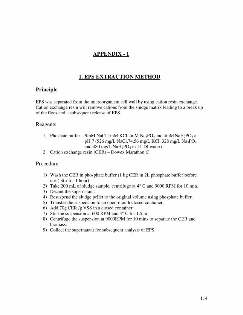
114
APPENDIX - 1
1. EPS EXTRACTION METHOD Principle EPS was separated from the microorganism cell wall by using cation resin exchange. Cation exchange resin will remove cations from the sludge matrix leading to a break up of the flocs and a subsequent release of EPS. Reagents
1. Phoshate buffer – 9mM NaCl,1mM KCl,2mM Na3PO4 and 4mM NaH2PO4 at pH 7 (526 mg/L NaCl,74.56 mg/L KCl, 328 mg/L Na3PO4 and 480 mg/L NaH2PO4 in 1L DI water)
2. Cation exchange resin (CER) – Dowex Marathon C Procedure
1) Wash the CER in phosphate buffer (1 kg CER in 2L phosphate buffer)before use.( Stir for 1 hour)
2) Take 200 mL of sludge sample, centrifuge at 4° C and 9000 RPM for 10 min. 3) Decant the supernatant. 4) Resuspend the sludge pellet to the original volume using phosphate buffer. 5) Transfer the suspension to an open-mouth closed container. 6) Add 70g CER /g VSS in a closed container. 7) Stir the suspension at 600 RPM and 4° C for 1.5 hr. 8) Centrifuge the suspension at 9000RPM for 10 mins to separate the CER and
biomass. 9) Collect the supernatant for subsequent analysis of EPS.
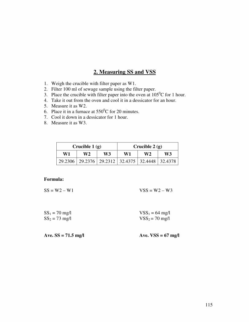
115
2. Measuring SS and VSS
1. Weigh the crucible with filter paper as W1. 2. Filter 100 ml of sewage sample using the filter paper. 3. Place the crucible with filter paper into the oven at 1050C for 1 hour. 4. Take it out from the oven and cool it in a dessicator for an hour. 5. Measure it as W2. 6. Place it in a furnace at 5500C for 20 minutes. 7. Cool it down in a dessicator for 1 hour. 8. Measure it as W3.
Crucible 1 (g) Crucible 2 (g) W1 W2 W3 W1 W2 W3
29.2306 29.2376 29.2312 32.4375 32.4448 32.4378 Formula: SS = W2 – W1 VSS = W2 – W3 SS1 = 70 mg/l VSS1 = 64 mg/l SS2 = 73 mg/l VSS2 = 70 mg/l
Ave. SS = 71.5 mg/l Ave. VSS = 67 mg/l