feasibility study of solar-wind hybrid power system for ...877768/fulltext01.pdf · master of...
TRANSCRIPT

Master of Science Thesis KTH School of Industrial Engineering and Management
Energy Technology EGI-2015-033MSC EKV1089 Division of Heat and Power
SE-100 44 STOCKHOLM
Feasibility Study of Solar-Wind Hybrid Power System for Rural Electrification at the
Estatuene Locality in Mozambique
Berino Francisco Silinto
Nelso Alberto Bila

i
Master of Science Thesis EGI-2015-033MSC EKV1089
Feasibility Study of Solar-Wind Hybrid Power System for Rural Electrification at the Estatuene Locality
in Mozambique
Berino Francisco Silinto & Nelso Alberto Bila
Approved
2015-11-25
Examiner
Miroslav Petrov – KTH/ITM/EGI
Supervisor
Miroslav Petrov
Commissioner
University Eduardo Mondlane, Maputo
Contact person at UEM
Dr. Geraldo Nhumaio
ABSTRACT
This project work focuses on the feasibility study of a hybrid PV-Wind System for rural electrification at
the Estatuene Locality in southern Mozambique. This is in line with electricity network expansion, which,
in Mozambique shows high implementation cost and low operation cost. Through field research, an
analysis was made of the actual electrical demand in the Estatuene rural community. The wind data was
collected from the installed weather stations in the region while the solar data were extracted internally
from the HOMER software by introducing the site coordinates.
All the configurations, simulations and selection of hybrid systems were also made using HOMER. For
the Estatuene rural community it was estimated a scaled annual average demand of 9.4 kWh/day with a
peak load of 1.4 kW for DC charge; and a total scaled annual average of 133 kWh/day with a peak load of
15.3 kW for AC Charge. The annual mean solar potential is 5.205 kWh/m2/d, and the mean wind speed
is 4.84 m/s for 12 meters above the ground. Thus the calculations and the selection of the best
configuration of the hybrid system were crossed out with the technical specifications and costs of
photovoltaic panels, wind turbines, power converter, batteries, and the electricity network, specifically for
the comparison between an optimum hybrid system solution and two separate ones. The calculations
presented an analysis of the technical and the financial viability of the selected hybrid system for local
electric power production.
Keywords: hybrid system, solar power, PV, wind power, rural electrification, computational simulation,
feasibility analysis, sustainable development.

ii
ACKNOWLEDGMENT
It’s our pleasure to thank to all SEE professors that gave us assistance during the course and transmitted their knowledge shaping us what we are today. Special thanks goes to our scientific supervisor’s, Geraldo Nhumaio (Phd) and Miroslav Petrov (Phd) for their assistance during the conception, revision, corrections of this thesis and especially for understanding, patience and acceptance of our limitations as students. Our family for their patience and acceptance along the time that we weren’t able to be with them. Our gratitude to Estatuene local authorities for their time and patience during community data surveys. Thanks to Dra. Miquelina Menenses (FUNAE, CEO) for her authorization and letting us to use FUNAE meteorological Data.
Thanks to God for giving us health and energy to work on this thesis.

iii
TABLE OF CONTENTS
ABSTRACT ................................................................................................................................................... i ACKNOWLEDGMENT .......................................................................................................................... ii LIST OF FIGURES ................................................................................................................................... vi LIST OF TABLES .................................................................................................................................... vii NOMENCLATURE................................................................................................................................ viii ACRONYMS AND ABREVIATIONS ................................................................................................. ix
1 CHAPTER ONE: INTRODUCTION .......................................................................................... 1
1.1 Background to the study .......................................................................................................... 1
1.2 Statement of the Problem ........................................................................................................ 1
1.3 Objectives ................................................................................................................................ 2
1.3.1 General Objectives ............................................................................................................... 2
1.3.2 Specific Objectives ............................................................................................................... 2
1.4 Methodology and Structure of the Thesis ................................................................................. 3
2 CHAPTER TWO: LITERATURE REVIEW ............................................................................... 4
2.1 The Solar Energy Resource ...................................................................................................... 4
2.1.1 Thermal Conversion ............................................................................................................. 4
2.1.2 Photoelectric Conversion ..................................................................................................... 4
2.1.3 The Photovoltaic System ...................................................................................................... 4
2.1.4 Solar Cell Architecture ......................................................................................................... 5
2.1.5 Operation of Silicon Cells .................................................................................................... 5
2.1.6 Factors that Influence the Operation of a Solar Module ....................................................... 9
2.1.7 Solar Panel Orientation Angles ........................................................................................... 10
2.1.8 Solar panel circuit connections ........................................................................................... 10
2.2 The Wind Energy Resource .................................................................................................... 11
2.2.1 History of Wind Uses ......................................................................................................... 11
2.2.2 Wind Turbines: working principles ..................................................................................... 12
2.2.3 Power Output Control ....................................................................................................... 13
2.2.4 Wind Power Generation Technology ................................................................................. 15

iv
2.2.5 Wind Power Conversion .................................................................................................... 15
2.2.6 Prediction Models For Wind Resource ............................................................................... 17
2.2.7 Factors that Affect the Wind Characteristics (Speed and Power) ........................................ 19
2.3 Energy Storage (Battery types and operation) ......................................................................... 21
2.3.1 Types of Batteries............................................................................................................... 21
2.3.2 Key Battery Parameters and Characteristics ........................................................................ 22
2.4 Inverters and Charge Controllers ............................................................................................ 23
2.5 Evaluation of Solar Energy and Wind Energy Resources ........................................................ 24
2.5.1 Electricity Supply Through Hybrid Power Systems............................................................. 24
2.5.2 Advantages of Hybrid Power Systems ................................................................................. 25
2.6 The Local Study Area (Mozambique) ..................................................................................... 25
2.6.1 Geographical Location and Climate .................................................................................... 25
2.7 Mozambique Energy Profile ................................................................................................... 26
2.7.1 Solar Radiation and Wind Regime, Distribution and its Potential........................................ 27
2.7.2 Institutional Framework of the Energy Sector .................................................................... 29
3 CHAPTER THREE: MODELLING SOFTWARE, LOCAL DATA AND RESEARCH METHODOLOGY .................................................................................................................................. 31
3.1 Specific Study Area Description ............................................................................................. 31
3.2 Modelling Software: HOMER ................................................................................................ 31
3.3 Data and Modelling Approach ............................................................................................... 32
3.3.1 Data Survey and Analysis of the Electric Power Curve of the Load Demand ..................... 33
3.3.2 Analysis of solar and wind potential at Estatuene Region ................................................... 36
3.3.3 Analysis of Technological and Financial Resources used for the Feasibility of Hybrid Systems .......................................................................................................................................... 38
3.4 Specification of the configurations for the sensitivity analysis and simulations ........................ 40
4 CHAPTER FOUR: RESULTS AND DISCUSSION ................................................................ 41
4.1 Optimization and Modelling ................................................................................................... 41
4.1.1 Hybrid Energy System Configuration ................................................................................. 41
4.1.2 The Seasonal Load Demand Profile ................................................................................... 41
4.1.3 Results Obtained in the Simulations ................................................................................... 42
4.2 Economic and Technical Analysis of the Results .................................................................... 43
4.2.1 Economic Analysis ............................................................................................................. 43
4.2.2 Technical Analysis .............................................................................................................. 44

v
5 CHAPTER FIVE: CONCLUSIONS AND RECOMMENDATIONS ................................. 47
5.1 Conclusions ........................................................................................................................... 47
5.2 Recommendations and future work ........................................................................................ 48
LITERATURE........................................................................................................................................... 49
APPENDICES .......................................................................................................................................... 52
Appendix 1: FUNAE 4kW mini PV systems & Typical electrified Infrastructures/Households. 52
Appendix 2: FUNAE Solar modules Characteristics ........................................................................... 52
Appendix 3: Wind Turbines - FD6.4-5000 and FD8.0-10000 Characteristics ................................. 53
Appendix 5: Batteries (2v, OPZS3500, 3000Ah) .................................................................................. 54
Appendix 6: Overall optimization results in HOMER ........................................................................ 55
Appendix 7: Scenario 1, 2 and 3 System Report ................................................................................... 60

vi
LIST OF FIGURES
Figure 2. 1: Efficiency of some semiconductor materials. ............................................................ 5 Figure 2. 2: P-N junction. ........................................................................................................... 6 Figure 2. 3: Band diagram of a silicon solar cell, under illumination. ............................................ 7 Figure 2. 4: Simplified diagram of an equivalent solar cell circuit ................................................. 7 Figure 2. 5: I-V and P-V curves of a solar cell. Source: ................................................................ 8 Figure 2. 6: Simplified equivalent real solar cell ............................................................................ 9 Figure 2. 7: The geometry of installation of solar panel ............................................................. 10 Figure 2.8: Connections of solar modules in series-parallel ........................................................ 11 Figure 2. 9: Types of rotors according to the orientation of its axis. (a) Darrieus rotor - Vertical Axis (b) Savonius rotor - vertical axis, and (C) horizontais axis. ................................................. 12 Figure 2. 10: Diagram of parts that constitute a wind turbine. . ................................................. 13 Figure 2. 11: (a) Direction per sector (b) average speed by sector (c) energy per sector .............. 15 Figure 2. 12: Flow of wind through a cylinder/rotor of area (A) and length. ............................. 15 Figure 2. 13: a) Wind speed duration curves according to the Weibull distribution model. b) Wind speed frequency distribution. ........................................................................................... 17 Figure 2. 14: Variation of wind velocity with height above the ground. .................................... 19 Figure 2. 15: Different types of deep discharge batteries. ........................................................... 22 Figure 2. 16: Stand-alone hybrid system schematic configuration with AC energy bus. .............. 24 Figure 2. 17: Map of Mozambique. ........................................................................................... 26 Figure 2. 18: Solar radiation distribution for Mozambique. ........................................................ 28 Figure 2. 19: Mozambique annual wind distribution. ................................................................. 28
Figure 3. 1: Satellite image of the village. Source: www.googleearth.com ................................... 31 Figure 3. 2: Graphical view of daily energy demand ................................................................... 35 Figure 3. 3: Location map and measurement mast of the meteorological station ...................... 36 Figure 3. 4: Representation of the monthly mean wind speed (m/s) at 20 meters above ground level in the area of Estatuene. .................................................................................................... 37 Figure 3. 5: Estimate of solar radiation potential of the area of Estatuene on 10/03/2014 ........ 37 Figure 3. 6: Estatuene wind prevailing direction. ....................................................................... 39
Figure 4. 1: Configuration of the system in HOMER ............................................................... 41 Figure 4. 2: Peak load profile for Estatuene Locality .................................................................. 42 Figure 4. 3: Cost summary for the proposed systems. ................................................................ 43 Figure 4. 4: Cash flow summary for the three selected scenarios. ............................................... 44 Figure 4. 5: Technical evaluation ............................................................................................... 45 Figure 4. 6: Battery state of charge ............................................................................................ 46
vii
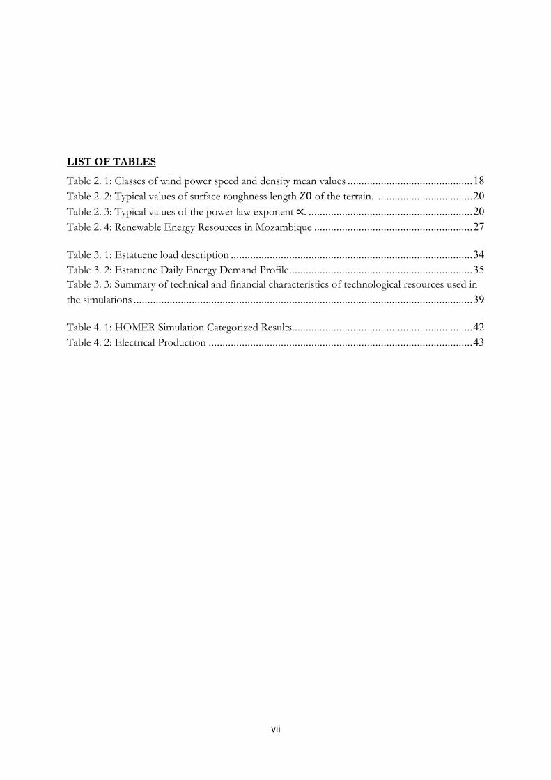
LIST OF TABLES
Table 2. 1: Classes of wind power speed and density mean values ............................................. 18 Table 2. 2: Typical values of surface roughness length 𝑍0 of the terrain. .................................. 20 Table 2. 3: Typical values of the power law exponent ∝. ........................................................... 20 Table 2. 4: Renewable Energy Resources in Mozambique ......................................................... 27 Table 3. 1: Estatuene load description ....................................................................................... 34 Table 3. 2: Estatuene Daily Energy Demand Profile .................................................................. 35 Table 3. 3: Summary of technical and financial characteristics of technological resources used in the simulations .......................................................................................................................... 39 Table 4. 1: HOMER Simulation Categorized Results................................................................. 42 Table 4. 2: Electrical Production ............................................................................................... 43

viii
NOMENCLATURE Symbol Description Unit A Cross section area of the cylinder [m2] Cp Betz limit Constant --- E Electric field [N/c] Eg Semiconductor Energy Band gap [N/c] f Frequency [Hz] F (V) Weibull probability distribution function --- G Solar irradiance [W/m] I Electric current feeding the load [A] I0 Reverse Diode current [A] Id Diod current [A] IMPP Current at maximum power point [A] Isc Short circuit current [A] JD Diffusion Current [A] K Boltzman Constant [J/k] k Shape factor --- L Length of the cylinder [m] ṁ Air mass flow [kg/s] m Diode ideality factor --- ƞ Conversion efficiency --- n, p types Semiconductor materials --- nn Electron concentration --- np Hole concentration --- P Power [W] PMPP Power at maximum power point [Wp] Ps Power density [W] q Electron charge [c] R Blade radius [m] Rp Parallel resistance [Ω] Rs Series Resistance [Ω] T Absolute temperature [oK] Ta Ambient temperature [oK] Tc Cell temperature [oK] v Velocity [m/s] V(z) Wind speed at height z [m/s] Vd Diode voltage [V] VMPP Voltage at maximum power point [V] vo Oncoming wind speed [m/s] Voc Open circuit voltage [V] Zo Surface roughness length [m] α Terrain roughness --- β Tilt angle of solar collector [oDegree] γ Solar altitude angle [oDegree] ϑ Rotor tip speed [m/s] λo Tip speed ratio --- ρ Air flow density [kg/m3] ω Angular velocity [rad/s]
ix
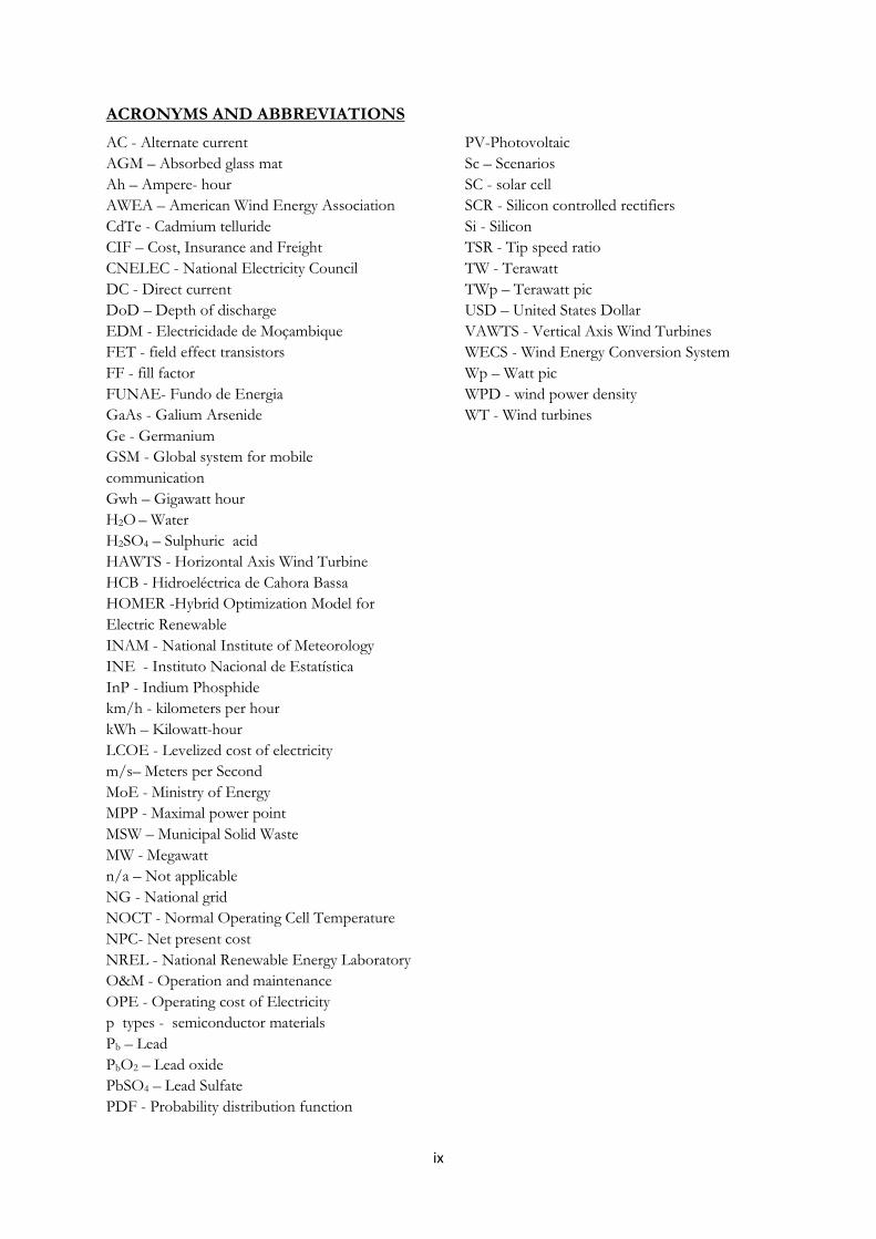
ACRONYMS AND ABBREVIATIONS AC - Alternate current AGM – Absorbed glass mat Ah – Ampere- hour AWEA – American Wind Energy Association CdTe - Cadmium telluride CIF – Cost, Insurance and Freight CNELEC - National Electricity Council DC - Direct current DoD – Depth of discharge EDM - Electricidade de Moçambique FET - field effect transistors FF - fill factor FUNAE- Fundo de Energia GaAs - Galium Arsenide Ge - Germanium GSM - Global system for mobile communication Gwh – Gigawatt hour H2O – Water H2SO4 – Sulphuric acid HAWTS - Horizontal Axis Wind Turbine HCB - Hidroeléctrica de Cahora Bassa HOMER -Hybrid Optimization Model for Electric Renewable INAM - National Institute of Meteorology INE - Instituto Nacional de Estatística InP - Indium Phosphide km/h - kilometers per hour kWh – Kilowatt-hour LCOE - Levelized cost of electricity m/s– Meters per Second MoE - Ministry of Energy MPP - Maximal power point MSW – Municipal Solid Waste MW - Megawatt n/a – Not applicable NG - National grid NOCT - Normal Operating Cell Temperature NPC- Net present cost NREL - National Renewable Energy Laboratory O&M - Operation and maintenance OPE - Operating cost of Electricity p types - semiconductor materials Pb – Lead PbO2 – Lead oxide PbSO4 – Lead Sulfate PDF - Probability distribution function
PV-Photovoltaic Sc – Scenarios SC - solar cell SCR - Silicon controlled rectifiers Si - Silicon TSR - Tip speed ratio TW - Terawatt TWp – Terawatt pic USD – United States Dollar VAWTS - Vertical Axis Wind Turbines WECS - Wind Energy Conversion System Wp – Watt pic WPD - wind power density WT - Wind turbines

1
1 CHAPTER ONE: INTRODUCTION
1.1 Background to the study
At present, the increasing consumption of electricity drives the development of different forms of energy
use around the world. This demand for electricity has been supplied mostly by fossil sources of energy.
With high impact on the world economy caused by the increasing price fluctuations of fossil fuels, due to
geopolitical issues and/or environmental disasters, the search for solutions that promote the sustainability
of the current lifestyle of societies is growing in importance, which can bridge the rapidly growing energy
demand in emerging economies such as Mozambique.
In Mozambique, the electricity supply is mainly realized through transmission lines, thus creating
difficulties in meeting the distant or remote regions that due to orographic characteristics of places where
people live, or geographical isolation, are not yet connected to the conventional national grid, as the
population density to be supplied is low and do not justify large investments that represents the grid
expansion, costs of network lines and power distribution maintenance.
The remote regions of the country are basically powered by isolated generator set systems. Despite of
having relatively low cost, these systems are not the best solution for remote areas as they require a
regular maintenance program that is rarely executed, leading to increased number of failures of the
generators, which is reflected in a high rate of unavailability factors. This situation is also due to the
increased fuel costs, especially regarding distant areas with a high shipping cost, which inflates the cost of
electricity delivered by these systems.
Thus, this work aims to study the feasibility of a wind-PV hybrid system for local electricity production
in order to power rural communities and to determine the circumstances in which a system of this nature
becomes economically feasible for a specific site in rural Mozambique. 1.2 Statement of the Problem
Mozambique is a country located on the African Continent, which has 10 provinces and 129 districts. The
total population is estimated to be approximately 22 million, with about 80% living in rural or suburban
areas, grouped in small communities spread all over the country (INE, 2007) and their domestic primary
energy needs are fully satisfied on the basis of firewood and charcoal (Cuamba, et al., 2006).
The country is rich in modern energy resources, however, more than 80% of the country’s population is
not connected to the national grid because of their location (rural areas) and poor economy, lack of basic
infrastructure, high initial investment and costs of the transmission and distribution lines from the central

2
locations to remote areas which are considerably high. This situation leads to many remote areas
remaining out of the reach of the centralized electrical grid long into the future (Hankins, 2009)
The electricity industry in Mozambique is presently represented by two major companies that include the
hydropower producer “Hidroeléctrica de Cahora Bassa” (HCB) and the centralized electricity utility
“Electricidade de Moçambique” (EDM). HCB generates over 90% of the country’s electricity at Cahora
Bassa Dam and exports the bulk of this to South Africa. EDM has some limited generation capacity and
buys most of its electricity from HCB. EDM is responsible for the management, maintenance and
development of the national grid, including transmission and distribution lines. (Hankins, 2009)
The Mozambican Government set up in 1998 a new institution, named FUNAE (Fundo Nacional de
Energia), to solve problems of off-grid energy demand and rural electrification. Since then FUNAE in
the context of its supervision and financing of energy related projects, had the most impact on renewable
energy development and initiative in promoting the use of stand-alone PV systems to supply electricity to
small villages, community schools, health centres and local governmental services.
FUNAE is installing small power plants of primarily stand-alone PV systems with 4kW in small villages to
electrify surrounding areas (usually within 300 meters) such as health centers, schools, police stations and
households; and also have awarded a consultancy for a company “Gesto Energy” (Portuguese consultant)
to map out the existing renewable energy sources - Solar, Wind, Hydro, Biomass, Municipal Solid Waste
(MSW), Geothermal and Wave energy - over the country in order to prioritize the best renewable projects
in Mozambique. Under the auspices of this consultancy some equipment to collect wind and solar data
were installed over the country, whose readings will be used in the present study.
The combination of solar PV and Wind turbine hybrid systems is new in Mozambique (not yet
implemented) and from the literature it’s seen that hybrids can be more cost effective than PV-alone or
Wind-alone systems (Pazmino, 2007) by reducing the energy storage requirements. The present work
attempts to investigate the possibility of providing electricity from Wind-Solar hybrid power system to a
remotely located village that is outside of the main grid.
1.3 Objectives
1.3.1 General Objectives • To study the feasibility of solar-wind hybrid power systems for rural electrification in
Mozambique.
1.3.2 Specific Objectives • To analyse and evaluate the renewable energy potential mainly for those two resources, solar and
wind, at the Estatuene Locality in southern Mozambique;

3
• To make the prefeasibility analysis and estimate the load demand;
• To assess the technical feasibility of a hybrid solar-wind power system to meet the load
requirements of the specific remote village electrification.
• To evaluate a strategy to optimize the size of the energy generation and storage subsystems;
• To assess techno-economic approach for determination of a system that guarantees the energy
supply by the hybrid system with a lowest investment; and
• To analyse the effect of load size or load variation and at what extent the combination of the
hybrid energy systems can reduce the costs if compared to a PV-only or Wind-only standalone
off-grid system.
1.4 Methodology and Structure of the Thesis
This report is divided into five chapters. Chapter One is an introduction to the study, where the problem,
justification, the aim and objectives of the study are outlined. Chapter Two is devoted to a theoretical
discussion and literature review about the means of harnessing solar radiation and wind resources for
energy applications, and their use as resource for energy production and leveraging them to generate
electricity. Some techniques are also explored for the estimation of the available and extractable energy
from these renewable sources and the factors that may affect their potential. The chapter is finalized with
presentation of the energy profile of Mozambique.
Chapter Three presents the modelling approach used in this study by describing all the methodological
procedures taken in place; then followed by Chapter Four where the results of the simulations and
analysis are brought up and discussed, for identifying the best option for electrification of the chosen
rural community of Estatuene.
Finally, in Chapter Five some important conclusions are drawn, together with general recommendations
for future research and practical implementation.
The thesis work was carried out by a team of two students: Berino Silinto and Nelso Bila. The team
performed literature review in books, papers, internet sources etc, where: Nelso were responsible for
surveying information regarding solar resource, storage systems, inverters; and Berino for wind resource,
hybrid systems, Mozambique energy profile. Both students worked together on the surveys of technical
data and equipment characteristics (for wind turbines, photovoltaic panels, battery banks for electrical
energy storage, converters/charge controllers, etc.), data analyses, discussion and results.

4
2 CHAPTER TWO: LITERATURE REVIEW
2.1 The Solar Energy Resource
The sun is the main energy source which is responsible for supporting all life activity around the world,
such as the Earth’s thermal comfort, photosynthesis in plants and the whole biogeochemical system. The
sun emits its energy in form of electromagnetic radiation and after reaching the earth surface it is
converted to other types of energy sources and used for many purposes.
The human beings are using the energy from the Sun in two main ways, i.e. for photo-electric generation
and thermal conversion. These applications represent one big leap for the solution of the world energy
shortage. For example, it is estimated that out of 1.76x10¹⁵ TW of raw solar energy striking the Earth, 60
TW can be economically converted into electricity and, considering that the estimation of the world
energy demand until 2050 is about 25-30 TW, it is clear that only solar energy is enough to supply all
demand and to free the world of fossil fuels (Kalogirou, 2009).
2.1.1 Thermal Conversion
The methods of thermal conversion of solar energy are based on absorption of radiant energy by black
body surface. This can be a complex process, which varies according to the type of absorbent material.
Involves diffusion photon absorption, electron acceleration, multiple collisions, but the final effect is the
heating, or radiant energy of all qualities are transformed into heat represented by the increase in
temperature. For instance, collectors can be used to gather solar radiation to produce temperature high
enough to be used directly or further converted to electricity via thermomechanical processes such as for
example a steam turbine cycle (Chen, 2011).
2.1.2 Photoelectric Conversion
This fundamental photoelectric conversion consists of the escape of electrons (electric current) from the
clear metal surface when the light with certain frequency strikes on this surface.
2.1.3 The Photovoltaic System
A PV system is a composition of all the devices used to convert solar photons directly into electricity
which are: Solar panel, storage unit, charge/discharge regulator and inverter if necessary to convert direct
current (DC) to alternating current (AC). In some cases, depending on the purpose storage might not be
necessary (e.g. connection to the grid). The key element of a PV system is the solar cell. This element is
responsible for the conversion of solar radiation into electricity and its function is based on the
photoelectric effect1 that consists on electrical generation by certain materials when exposed to the light.
1) Discovered by French physicist Edmond Becquerel in 1839

5
The first silicon solar cell (SC) was discovered by a French physicist, Edmond Becquerel in 1839.
Becquerel experiments showed that certain materials produce a small amount of electricity when exposed
to the light. This effect was firstly studied in metals such as silicon with performance of about 2%. The
research proceeded and in 1954 was achieved a silicon solar cell with an efficiency of about 6%, reported
by Chapin, Fuller and Pearson (Chen, 2011). Regarding its application, the SC’s were firstly used to charge
batteries of the United States Satellite (U.S. Vanguard) in 1958 (Maini, et al., 2011).
Due to high costs, the SC’s were initially used only for space, military and scientific research purposes.
However, with the energy crisis starting in the 1970’s, interest emerged in developing of SC’s for civilian
purposes (Kalogirou, 2009).
2.1.4 Solar Cell Architecture
The SC’s can be manufactured using different types of semiconductor materials, such as Silicon (Si),
Germanium (Ge), Indium Phosphide (InP), Gallium Arsenide (GaAs), Cadmium telluride (CdTe), etc.,
but some of these materials (e.g. InP, GaAs) are not abundant in the Earth and therefore are much
expensive if compared to those such as Si and Ge which leads to the prevailing usage of Si in commercial
applications. The Ge is not much used because of its lower efficiency as can be seen in figure 2.1 below.
Figure 2. 1: Efficiency potential of some semiconductor materials. Source: (LEM, 2014)
2.1.5 Operation of Silicon Cells
SC is a junction of two types of materials, i.e. the n and p types of semiconductor materials. When those
are joined together, free electrons in the n-type material move to the p-type material and also free holes
from p-type material move to n-type material resembling the flow of electric charges, creating the so-
called diffusion current (JD). (Kalogirou, 2009).

6
When the charge carriers (electrons and holes) move from one side to another, they leave behind both
donor and acceptor ions on their previous material (UNICAMP, 2014). Those left ions create spatial
charges and, consequently there is an electric potential given by the following expression.
𝑉 = 𝐾𝐾𝑞𝑙𝑙 𝑛𝑛
𝑛𝑝 (1)
Where 𝑙𝑛 is the electron concentration and 𝑙𝑝 is the holes concentration, K- Boltzmann constant
(1.38 ∗ 10−23 𝐽𝐾
), q- Electron charge (1.6 ∗ 10−19 𝑐) and T is the absolute temperature given in [0K]. As electric field is gradient of electric potential, it yields to the following expression (Luque, et al., 2011) and (UNICAMP, 2014).
𝐸 = 𝐾𝐾𝑞
1𝑛∇𝑙 (2)
Where 𝑬 is the Electric field given by [Newton/Coulomb].
The electric field due to the existence of spatial charges on a p-n junction, leads into the drift current
(“diffusion force” on holes) with opposite direction to the diffusion current (“diffusion force” on
electrons). Thus, the appearance of drift current stops the diffusion of charge carriers from one side to
another and the junction works as a dielectric as is shown in figure 2.2.
Figure 2. 2: P-N junction. Source: (TheNoise, 2007)
The electric field built up on junction that is yielded within the electric potential, disables the flux of
charge carriers through it. However, it is of extreme importance to direct the charge carriers when they
reach the depletion zone after they are excited by an external source (i.e. sunlight or thermal excitation).
The theory of light set up two important conclusions that instead of electromagnetic wave is also a joint
of particles called photons. So, if those photons fall within the p-n junction, different situations such as
electron-hole pair creation and recombination can take place according to their energy if compared to the
semiconductor band gap (Eg).

7
If the energy of the photon that falls within the p-n junction is equal or more than Eg, after transferring
this energy to the electron, it can jump into the conduction band and, due to electric dipole in depletion
zone, electron can be directed to n-type material and the hole, to the p-type material (Yu, et al., 2010)
Figure 2. 3: Band diagram of a silicon solar cell, under illumination. Source: (Wikpedia, 2014)
The analysis of SC’s functionality can be stated using two models: the first is related with a single diode
model and the second to two diode model. However for the next steps we’re revising the single diode
model given that the second is more labour-intensive and is only used for full understanding of the
behaviour of SC’s (Haberlin, 2012).
In the single diode model there are two modes of functioning of the SC’s, namely the ideal SC in which
there are no crystal defects and, the second is related to the real SC in which crystal defects are taken into
account.
a) The ideal SC is represented by a diode of three parameters: the short circuit current (Isc), the diode current (Id) and the current feeding the load (I).
In figure 2.4 below is presented a simplified diagram of an equivalent circuit of an ideal SC in which is taken into account that there is no voltage and current drop.
Figure 2. 4: Simplified diagram of an equivalent solar cell circuit
Applying the Kirchhoff’s law to the blue node of the equivalent SC in the figure above, the short circuit current is given by:
𝑰𝒔𝒔 = 𝐈 + 𝑰𝟎 𝐞𝒒𝒒𝒅𝐦𝐦𝐦 − 𝟏 (3)

8
Where 𝑰𝟎 is the diode reverse saturation current; 𝒒𝒅 is the voltage across the junction; m is the diode
ideality factor. The current flowing across the diode (𝑰𝒅 ) is given by the term of (3), 𝑰𝟎 𝐞𝒒𝒒𝒅𝐦𝐦𝐦 − 𝟏
There are two operating points of the solar cell, that can be obtained from the expression (3), in such a
way that:
For short circuit (𝑉𝑑 = 0 leading to 𝐼𝑑 = 0), thus:
𝐼𝑠𝑠 = I (4)
- For open circuit (𝑉𝑑 = 𝑉𝑜𝑠 , I = 0 )
From equation (3) we get:
𝑉𝑉𝑐 = 𝑚𝑚𝐾𝑞
ln 𝐼𝑠𝑠𝐼𝑜
+ 1 (5)
The open circuit voltage 𝑉𝑜𝑠 and short circuit current 𝐼𝑠𝑠 are parameters given by the manufacturer and
are very important to draw the I-V curve, given below (Figure 2.5), which is used to predict the SC’s
performance at various temperatures, voltage loads and level of insolation (Yu, et al., 2010)
Figure 2. 5: I-V and P-V curves of a solar cell. Source: (Luque, et al., 2011)
The main important point in this curve is MPP (maximal power point) that is the point in which the
module produces the greatest power, it is always found where the curve begins to bend and defines the
outputs of the module (VMPP – Voltage at maximum power point and IMPP – Current at maximum power
point). The power output at any other point is less than the power at maximum power point (PMPP).
However, there is another parameter that describes the deviation of the I-V curve in relation to the ideal, called the Fill Factor (FF). The fill factor is the ratio of the maximum obtainable power to the product of the open-circuit voltage and short-circuit current, and is given by:

9
𝐹𝐹 = 𝐼𝑀𝑀𝑀.𝑉𝑀𝑀𝑀𝐼𝑠𝑠.𝑉𝑂𝑂
(6)
The conversion efficiency (η) of SC, is the power density delivered at the operating point as a fraction of the incident light power density Ps and is given by the equation:
η = FF.𝐼𝑀𝑀𝑀.𝑉𝑀𝑀𝑀𝑃𝑠
(7)
b) The Real Solar Cell Model
The analysis of the real solar cell is made taking into account all cell defects namely, imperfection of
semiconductor material defects, junction and metal contacts. These imperfections are clumped into Series
Resistance (Rs) and Parallel resistance (Rp) shown in the figure 2.6 below.
Figure 2. 6: Simplified equivalent real solar cell
Taking into account the figure above the short circuit current (Isc) from equation number 3 and the
current feeding the load can be transformed respectively to:
𝐼𝑆𝑠 = 𝐼𝑑+𝐼𝑝 + 𝐼
𝐼 = 𝐼𝐼𝑐 − 𝐼𝑉 𝑒𝑞(𝑉+𝐼𝐼𝑠)𝑚𝑚𝑚 − 1 − V+𝐼𝐼𝑠
R𝑝 (8)
2.1.6 Factors that Influence the Operation of a Solar Module
There are five major factors that can affect the solar cell performance namely:
a) The cell material: depending on the material and manufacturing method used, solar cells can
achieve different conversion efficiencies of light, for instance the efficiency of amorphous silicon
ranges from 5% to 7%, for the polycrystalline silicon, its efficiency does not exceed 12% and for the
mono crystalline silicon the efficiency is over 12% and not exceeding 18% (Electronica, 2014) and
(Seraphim, et al., 2004)
b) The radiation intensity on module output: the current output is proportional to the radiation
intensity, increasing the light intensity, the current also increases but the voltage does not change
considerably at I-V curve above. (Haberlin, 2012).
10
c) The heat on module output: The output voltage of the module is affected by increasing the
temperature of the module. At increasing temperature the voltage decreases considerably, however,
the current does not change significantly. According to (Haberlin, 2012), the variation of temperature
during the operation of a solar module may be explained by the equation below:
𝑇𝑠 − 𝑇𝑎 = (𝑁𝑁𝑁𝑇 − 20) 𝐺800
(9)
Where G is the solar irradiance [W/m2], Tc and Ta are the cell and ambient temperatures respectively,
“NOCT” is the Normal Operating Cell Temperature, its value is usually given by the manufacturer, and
ranges between 44-54oC for a conventional module, under the following conditions at open circuit:
GNOCT=800W/m2 of solar irradiance, Ta =200 c, air mass of 1.5 and Wind speed is 1 m/s.
d) The shading effect on module output: If a module or part of module (cell) is shaded, may partially
produce or even not produce electricity, and if it happens can also cause hot spots heating. However,
this fact can be mitigated installing bypass diodes (Stapleton, et al., 2012).
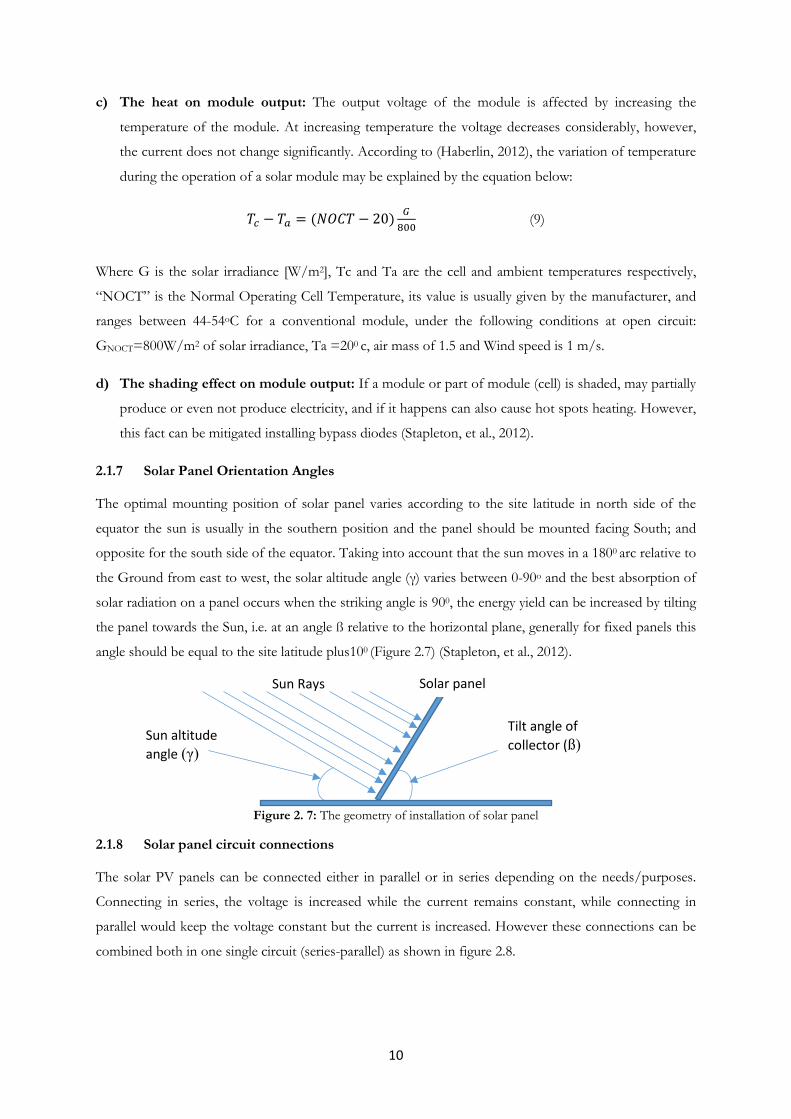
2.1.7 Solar Panel Orientation Angles
The optimal mounting position of solar panel varies according to the site latitude in north side of the
equator the sun is usually in the southern position and the panel should be mounted facing South; and
opposite for the south side of the equator. Taking into account that the sun moves in a 1800 arc relative to
the Ground from east to west, the solar altitude angle (γ) varies between 0-90o and the best absorption of
solar radiation on a panel occurs when the striking angle is 900, the energy yield can be increased by tilting
the panel towards the Sun, i.e. at an angle ß relative to the horizontal plane, generally for fixed panels this
angle should be equal to the site latitude plus100 (Figure 2.7) (Stapleton, et al., 2012).
Figure 2. 7: The geometry of installation of solar panel
2.1.8 Solar panel circuit connections
The solar PV panels can be connected either in parallel or in series depending on the needs/purposes.
Connecting in series, the voltage is increased while the current remains constant, while connecting in
parallel would keep the voltage constant but the current is increased. However these connections can be
combined both in one single circuit (series-parallel) as shown in figure 2.8.
Sun Rays
Tilt angle of collector (ß) Sun altitude
angle (γ)
Solar panel

11
Figure 2.8: Connections of solar modules in series-parallel
The connections and results obtained from the solar panels are the same for Batteries connections.
2.2 The Wind Energy Resource
The wind is an abundant, free, clean, sustainable and environmentally-friendly renewable energy source. It
has served the human civilization for many centuries by propelling ships and driving windmills to grind
grain and pump water, and nowadays also for electrical power production (Johnson, 2006).
2.2.1 History of Wind Uses
Wind as source of energy has been in use by humans for many centuries and for energy purposes dates
back five thousand (5000) years ago by sailing ships and boats used by the ancient Egyptians (Wortman,
1983), (Johnson, 2006). Its use occurs through the conversion of kinetic energy into a translational
kinetic energy of rotation, using wind turbines to generate electricity, or windmills for mechanical work to
pump water from deep wells (Burton, et al., 2011).
The first windmill machines were also used around 2000 years B.C., in ancient Babylon and China,
evolving since then to the modern wind turbines. In the western world the first application of windmills
was the grinding grain and pumping water from deep wells (Burton, et al., 2011), (IOWA, 2013) and
(Coalition, 2013).
The first modern wind turbine designed especially for electricity generation, was constructed in Denmark
in the early 1890 for supplying electricity to rural areas. In the same period a 12kW of power windmill was
constructed in the United States of America (USA). It was a large wind electric generator with 17 meters
diameter of rotor and 144 wooden propellers (Burton, et al., 2011).
The oil crisis in the 1970s sparked interest in wind energy in response to uncertainty of the price and
availability of fossil fuels. The wind turbine technology research and development programs that followed
this oil crisis during last century, introduced significant improvements resulting in modern computer

12
controlled wind turbines, which brought new and more efficient ways of converting wind energy into
useful mechanical or electrical power (Coalition, 2013), (Ahmed, 2011).
Nowadays the mankind is looking for new sources and technologies of energy that are inexpensive,
regarding the exhaustion of coal, oil and even radioactive materials. For this reason there is a multitudeof
scientific studies tending to better leverage inexhaustible sources of energy such as the renewables and the
solar and wind in particular.
2.2.2 Wind Turbines: working principles
Most wind turbines (WT) are machines built to convert the containing power in the wind into electricity.
The main classification of those machines is according to the interaction of their blades with the wind by
aerodynamic forces - drag or lift or a combination of both; and the orientation of the rotor axis with
respect to the ground and to the tower – upwind or downwind (Ahmed, 2011). According to the
orientation of the axis there are two types: The Horizontal Axis Wind Turbine, or HAWTS, and Vertical
Axis Wind Turbines, or VAWTS (Figure 2.10).
Among the VAWTs machines we highlight the Savonius (Figure 2.10 b) mostly used for water pumping
and the Darrieus (Figure 2.10 a) WT. They have the advantage of receiving wind from any direction not
requiring tracking mechanisms of the wind direction and that the coupling between the rotor and the
generator can be made at ground level, allowing easy access for maintenance meaning that smaller towers
gets reduced costs. The main disadvantage is that it has no self-starting, high torque fluctuations and
limited options of regulations at high wind speed.
a) b) c) Figure 2. 9: Types of rotors according to the orientation of its axis. (a) Darrieus rotor - Vertical Axis (b) H-type rotor - vertical axis, and (C) Upwind horizontais axis rotor. Source: (Burton, et al., 2011) and (IOWA, 2013),
The other type is the HAWT’s where the rotors are kept perpendicular to the wind and the rotational
driving force is lift and the blades can be in front (upwind) or behind (downwind) of the tower. The
HAWTs take advantage of extracting higher wind speeds farther from the ground as the rotors are placed
on the top of a tower.

13
Detailed explanation of the working mechanisms of both WTs types can be found in the literature such as (Manwell, et al., 2009), (Ackermann, et al., 2000), (Ahmed, 2011), (Burton, et al., 2011), etc.
In the present work we will focus on the HAWT’s with three blades attached to a central hub as it is the
most widespread in the wind power industry and in use today. Together, the blades and the hub form the
rotor (the main element to capture energy), which are connected to an electrical generator. When the
wind blows, the rotor turns and the generator produces alternating current (AC) electricity. WT with
multi-blade rotors (20 or more blades) have high starting torque in light wind and are mainly used for
mechanical water pumping.
The main configuration and components of the HAWT are shown in figure 2.11, which consists of a
tower and nacelle mounted at the top of a tower.
Figure 2. 10: Diagram of parts that constitute a wind turbine. Source: (Burton, et al., 2011).
The nacelle contains the main components of the WT such as: the electricity generator, gearbox and the
rotor. The generator transforms the rotational mechanical energy delivered by the gears, into electrical
energy. The generator may be of asynchronous, synchronous, direct current and alternating current
commutated types each having its advantages and disadvantages, the use of one type or the other will
depend on the turbine size or the specific application and on the preferences of the manufacturer of the
turbine (IOWA, 2013), (Burton, et al., 2011).
2.2.3 Power Output Control
Most of WT machines have control systems, composed of wind speed and direction measuring devices
(anemometers) and computer systems connected to sensors, valves, motors and pumps that monitor all
processes and trigger mechanisms across the turbine.

14
These control systems communicate with the operator via a communication link sending alarms or
requesting for services by means of radio, telephone and nowadays through the Internet. It also can
gather statistics or check the status of wind turbines.
The main mechanism to point here is yaw control that orients the turbine (points the nacelle) towards
wind direction or moves the nacelle out of the wind in case of high wind speeds in response to a signal
from the wind. For small WT, the rotor and the nacelle are oriented into the wind with a tail vane
(Ahmed, 2011).
There are other three principles of aerodynamic control, aiming to maximize the extraction of power
from wind turbines which are: The Passive Stall and, active Pitch Control, and active stall.
The passive stall control is a system which reacts according to the wind speed. In this system the blades
are fixed according to a given pitch angle so that there is a decrease in the aerodynamic forces of lift
coefficient and associated increase in drag coefficient when wind speeds above the rated speed are
achieved (Ahmed, 2011).
The active pitch control is a system requiring information from the control system via an anemometer
or other sensors installed in the turbine. The pitch control operates when the rated power of the turbine
(cutting speed) are exceeded, the rotor blades rotating around its axis, reducing the angle of attack of the
wind and thus the aerodynamic forces on the turbine, reducing the extracted power. The rotor blades are
rotated at certain angles, for each wind speed above to the rated power to continuously extract the rated
power (Ahmed, 2011).
The active stall control combines both pitch and stall control mechanisms. This type of control achieves
power limitations above the rated wind speed, by pitching the blades initially into stall, i.e. there is a small
turning of the blades (typically up to 5°) around its axis for certain speeds. The twists along the blades are
necessary with this type of control (Ahmed, 2011).
Three other factors on the turbines are important: the starting speed, the rated/nominal speed and cutting
speed where starting speed is the minimum wind speed needed to start moving the blades and start
producing some energy (Ahmed, 2011). The rated speed is the minimum speed at which the turbine is
designed to develop the rated power
And finally the wind turbines also have an aerodynamic braking systems provided on each blade so that in
strong winds the rotor can be cut off. Each WT comes with information on the cut-off speed, that is the
maximum speed at which the turbine ceases or decreases energy production, activating aerodynamic
control systems or brakes, avoiding damages into the turbine structure or in the electric distribution
system (IOWA, 2013), (Burton, et al., 2011).
15
2.2.4 Wind Power Generation Technology
The wind is considered as a vector defined by: the wind direction and wind speed. Wind direction is the
direction from which the wind blows and is expressed in degrees. The wind speed is expressed in meters
per second (m/s), kilometres per hour (km/h). Measure of wind strengths over a period of time and in
different directions can be well illustrated and analysed through a wind rose diagram. This diagram can
indicate the percentage of time for which we receive wind, speed and energy from a particular direction.
A typical wind rose is a circular display of how wind speed and direction are distributed at a given
location for a certain time period.
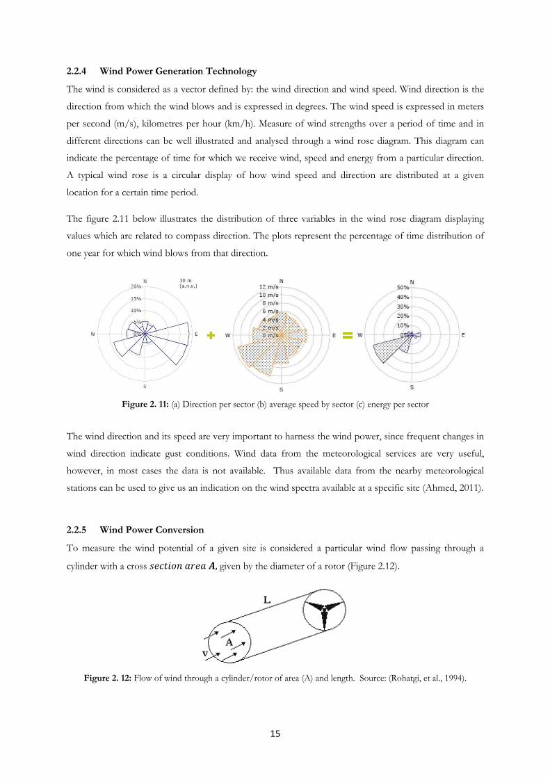
The figure 2.11 below illustrates the distribution of three variables in the wind rose diagram displaying
values which are related to compass direction. The plots represent the percentage of time distribution of
one year for which wind blows from that direction.
Figure 2. 11: (a) Direction per sector (b) average speed by sector (c) energy per sector
The wind direction and its speed are very important to harness the wind power, since frequent changes in
wind direction indicate gust conditions. Wind data from the meteorological services are very useful,
however, in most cases the data is not available. Thus available data from the nearby meteorological
stations can be used to give us an indication on the wind spectra available at a specific site (Ahmed, 2011).
2.2.5 Wind Power Conversion
To measure the wind potential of a given site is considered a particular wind flow passing through a
cylinder with a cross 𝐼𝑒𝑐𝑠𝑠𝑉𝑙 𝑎𝑎𝑒𝑎 𝑨, given by the diameter of a rotor (Figure 2.12).
Figure 2. 12: Flow of wind through a cylinder/rotor of area (A) and length. Source: (Rohatgi, et al., 1994).

16
According to the laws of physics, the rate of kinetic energy 𝑬 = 𝑷 𝑉𝑜 𝑠ℎ𝑒 𝑎𝑠𝑎 𝑚𝑎𝐼𝐼 𝑜𝑙𝑉𝑓 𝒎 𝑓𝑠𝑠ℎ a Speed V will be:
𝑃 = 12𝑉2 = 1
2(𝜌𝜌𝑉)𝑉2 (10)
Where is the mass flow rate of the air, ρ the air density (1.225 kg/m3 at sea level) that depends on
altitude and meteorological conditions - air pressure and temperature, both being functions of height
above sea level. (Walker, et al., 1997; Gipe, 2004) (Manwell, et al., 2009). The expression 1 represents the
total power which is given in Watts (W).
Considering a wind turbine placed inside of the cylinder, and part of the wind power will be transferred
and used by this wind turbine, then the power output “P” extracted by the rotor will be
𝑃 = 12𝑁𝑝𝜌𝜌𝑉3 (12)
Where Cp is a constant, dimensionless power coefficient or Betz limit, and is a measure of the efficiency
of the wind turbine in extracting the kinetic energy content of a wind stream that may be converted into
mechanical work, A is the rotor swept area. (Wortman, 1983); (Walker, et al., 1997) and (Twidell, et al.,
2006). It has a theoretical maximum value of 0.593, i.e, 𝑁𝑝 = 1627
= 0.593 = 59%.
On both expressions we can perceive that any increase in wind speed, will result in a substantial increase
of the power contained in the wind flow, but according to (Rohatgi, et al., 1994), only a part of the wind
power can be converted into a useful power, which in turn the available power from the wind turbine is
not limited only by the Betz coefficient but also on the aerodynamic and mechanical losses in the turbine
those related to rotation at the tip and base of the blade and the effect of the number of blades, as well
as on the limitation of the chosen rated generator capacity. The efficiency of mechanical equipment such
as the multiplier gearbox, the electrical generator and its coupling have to be considered.
Another important concept relating to power coefficient of wind turbine rotor is the optimal tip speed
ratio (TSR, λ0), that is, the ratio of the rotor tip speed to free wind speed. Rotor performance can be optimum
only for a unique tip speed ratio. The TSR of the rotor depends on the characteristics of the used blade
airfoil profile-blade radius “R”, oncoming wind speed 𝑉0, the angular velocity ω , the number of blades
“n” and the type of wind turbine (Twidell, et al., 2006).
In general, a three bladed wind turbine operates at a TSR between 6 and 8, with 7 being the most widely
reported value (Rageb, et al., 2011), (Twidell, et al., 2006) and (Ackermann, et al., 2000) thus the TSR is
dimensionless factor defined as:
TSR = λ0 = speed of rotor tip
𝑤𝑤𝑛𝑑 𝑠𝑝𝑠𝑠𝑑= ϑ
𝑉0= ωR
𝑉0 (13)
17
ωR𝑉0≈ 4π
𝑛, Where, 𝑉0 is the speed (m/sec) of the oncoming wind, ϑ is the rotor tip speed (m/sec), R is the
radius (m), ω = 2𝜋𝑜 is the angular velocity (rad/sec) and 𝑜is the rotational frequency (Hz), (1/sec).
2.2.6 Prediction Models For Wind Resource
The wind resource is very variable in nature. Combining meteorological and statistical techniques to
forecast wind can give us a very useful predictions for a specific wind farm power output project in which
will give us a best ideia to choose the appropriate Wind Energy Conversion System (WECS).
In the wind industry the Weibull probability distribution function (PDF) is commonly used. The Weibull
and Rayleigh PDFs are the most widely used PDFs to describe the wind speed distribution for WECS
applications (Ahmed, 2011) and (Twidell, et al., 2006).
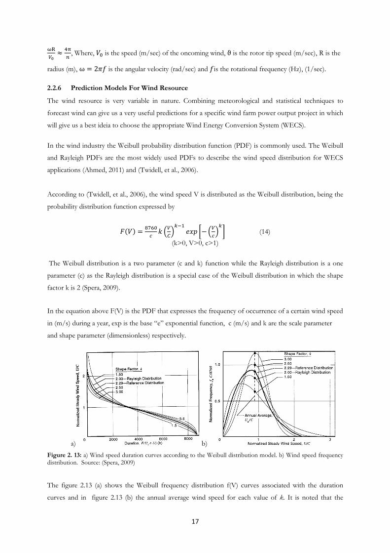
According to (Twidell, et al., 2006), the wind speed V is distributed as the Weibull distribution, being the
probability distribution function expressed by
𝐹(𝑉) = 8760𝑠𝑘 𝑉
𝐶𝑚−1
𝑒𝑒𝑒 −𝑉𝑠𝑚 (14)
(k>0, V>0, c>1)
The Weibull distribution is a two parameter (c and k) function while the Rayleigh distribution is a one
parameter (c) as the Rayleigh distribution is a special case of the Weibull distribution in which the shape
factor k is 2 (Spera, 2009).
In the equation above F(V) is the PDF that expresses the frequency of occurrence of a certain wind speed
in (m/s) during a year, exp is the base “e” exponential function, c (m/s) and k are the scale parameter
and shape parameter (dimensionless) respectively.
a) b)
Figure 2. 13: a) Wind speed duration curves according to the Weibull distribution model. b) Wind speed frequency distribution. Source: (Spera, 2009)
The figure 2.13 (a) shows the Weibull frequency distribution f(V) curves associated with the duration
curves and in figure 2.13 (b) the annual average wind speed for each value of k. It is noted that the

18
Weibull density function gets relatively narrower and more pinched as k gets larger. The peak also moves
in the direction of higher wind speeds as k increases.
According to (Manwell, et al., 2009), another important indication for wind energy resource evaluation of
a specific location’s wind energy characteristic is the mean wind power density (WPD), defined as the
wind power available per unit of swept area by the turbine blades and is tabulated for different heights
above ground and given by the following expression:
WPD=(𝑷𝐀
) = 𝝆𝒒𝟑
𝟐 or 𝑊𝑃𝑊 = 𝟏
𝟐𝟐∑ 𝝆𝒒𝒊𝟑𝒏𝒊=𝟏 ) (15)
Where n is the number of records in the averaging interval, ρ air density and 𝒒𝒊𝟑 the cube of the i th wind
speed value in W/m2
Changes in air velocity and its density affect the WPD. The table below shows the classes of wind power
density at 10m and 50 m2
Table 2. 1: Classes of wind power speed and density mean values 2. Source: (Ahmed, 2011) Wind power
class Description 10m 50m
Wind power density (Watts/m2)
Wind Speed (m/s)
Wind power density (Watts/m2)
Wind Speed (m/s)
1 Poor <100 <4.4 <200 <5.6 2 Marginal 100 - 150 4.4 - 5.1 200 - 300 5.6 - 6.4 3 Fair 150 - 200 5.1 - 5.6 300 - 400 6.4 - 7.0 4 Good 200 - 250 5.6 - 6.0 400 - 500 7.0 - 7.5 5 Excellent 250 - 300 6.0 – 6.4 500 - 600 7.5 - 8.0) 6 Outstanding 300 - 400 6.4 - 7.0 600 - 800 8.0 – 11.9 7 Superb >400 >7.0 >800 >11.9
Areas designated class 3 or greater are suitable for most utility-scale wind turbine applications, whereas
class 2 areas are marginal for utility-scale applications but may be suitable for rural applications. Class 1
areas are generally not suitable, although a few locations (e.g., exposed hilltops not shown on the maps)
with adequate wind resource for wind turbine applications may exist in some class 1 areas. The degree of
certainty with which the wind power class can be specified depends on three factors: the abundance and
quality of wind data; the complexity of the terrain; and the geographical variability of the resource.
Vertical extrapolation of wind speed is based on the 1/7 power law (NREL, 2014).
2) Vertical extrapolation of wind speed based on the 1/7 power law and Mean wind speed is based on the Rayleigh speed distribution of equivalent wind power density
19
2.2.7 Factors that Affect the Wind Characteristics (Speed and Power)
Boundary Layer Effects
The wind speed and its available power are very influenced by regional and local factors. The most
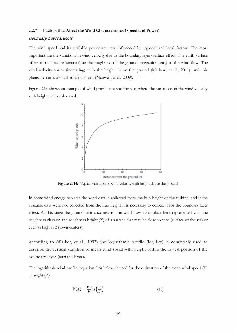
important are the variations in wind velocity due to the boundary layer/surface effect. The earth surface
offers a frictional resistance (due the roughness of the ground, vegetation, etc,) to the wind flow. The
wind velocity varies (increasing) with the height above the ground (Mathew, et al., 2011), and this
phenomenon is also called wind shear. (Manwell, et al., 2009).
Figure 2.14 shows an example of wind profile at a specific site, where the variations in the wind velocity
with height can be observed.
Figure 2. 14: Typical variation of wind velocity with height above the ground.
In some wind energy projects the wind data is collected from the hub height of the turbine, and if the
available data were not collected from the hub height it is necessary to correct it for the boundary layer
effect. At this stage the ground resistance against the wind flow takes place here represented with the
roughness class or the roughness height (Z) of a surface that may be close to zero (surface of the sea) or
even as high as 2 (town centers).
According to (Walker, et al., 1997) the logarithmic profile (log law) is commonly used to
describe the vertical variation of mean wind speed with height within the lowest portion of the
boundary layer (surface layer).
The logarithmic wind profile, equation (16) below, is used for the estimation of the mean wind speed (V)
at height (Z):
𝑉(𝑧) = 𝑉∗
𝑚ln 𝑍
𝑍0 (16)

20
Where 𝑉∗ is the friction velocity, 𝑘 is the Von Karman’s constant that is iqual to 0.4 and 𝑉(𝑧) is the
mean wind speed at height 𝑍 and 𝑍0 is the surface roughness length which characterizes the roughness
of the ground terrain.
Some typical values of approximate surface roughness lengths are given in Table 2.2.
Table 2. 2: Typical values of surface roughness length 𝑍0 of the terrain. Source: (Mathew, et al., 2011) Terrain Category Class Surface Landscape Description 𝒁𝟎 (m) 1 1 Sea Open sea, fetch at least 5 km 0.0002-0.005 1 2 Smooth Mud flats, snow, little vegetation, no obstacles 0.005 2 3 Open Flat terrain: grass, few isolated obstacles 0.025-0.1 3 4 Roughly Open Low crops: occasional large obstacles 0.1 3 5 Rough High Crops: scattered obstacles 0.2-0.3 3 6 Very Rough Orchards, bushes: numerous obstacles 0.5-1 4 7 Tall Forests, Dense Town Centers, etc. 1-2
The log law equation can be modified so that can be used to extrapolate from a reference height 𝑍𝑟 to
another level (to the hub height of the turbine for example) using the relationship:
𝑉(𝑧)𝑉(𝑍𝑟)
= ln 𝑍𝑍0 / ln 𝑍𝑟
𝑍0∝
(17)
Where 𝑉(𝑍𝑟) and 𝑉(𝑧) are the wind speeds at reference height (eg. 𝑍𝑟 = 10𝑚) and at the new height
(Z) respectively and 𝑍0 is the roughness length. Another approach that is used by many researchers
for a simple estimative of the distributions of mean wind speed with height is the empirical
model: power law (Walker, et al., 1997), given by:
𝑉(𝑧) = 𝑉(𝑧𝑟) 𝑍𝑍𝑟∝
(18)
where 𝑉(𝑧) is the needed wind velocity at elevation Z, 𝑉(𝑧𝑟) is the available mean wind velocity at the
known higher elevation Zr (=10m) and ∝ is the terrain roughness exponent and is also known as empirical
wind shear/power law exponent that is generally obtained experimentally from measurements of wind
speed at different heights and can be determined as:
∝=𝑙𝑜𝑙𝑉(𝑍𝑟)
𝑉𝑙𝑜𝑙𝑧𝑟𝑧 1
(19)
In assessing the potential energy of a wind turbine it is very important to convert or extrapolate the
available wind data to the height of the turbine rotor shaft. According to vertical extrapolation of wind
speed and under certain conditions ∝ is equal to 1/7, indicating a correspondence between wind profiles
and flow over flat terrain.
Table 2. 3: Typical values of the power law exponent ∝. Source: (Mathew, et al., 2011)
Terrain Category Class
Type of terrain
Landscape Description
∝
1 1 Sand 0.1 1 2 Mown grass 0.13 2 3 High grass 0.19 3 4 Suburb buildings 0.32
21
Two methods for modelling the vertical wind profile (the log and power laws) were discussed in this
section. Those laws are applicable for flat and homogenous terrains meaning that if we consider irregular
earth surfaces it is expected to have modifications to the wind flow mainly if we’re dealing with flat and
non-flat terrains. More detailed explanation of their effects to the wind flow can be found in literature.
2.3 Energy Storage (Battery types and operation)
One of the problems that energy production from renewable energy source sector faces, is to maintain
fixed or constant the amount of electricity produced over a certain period of time, even though knowing
that throughout the day electricity production and demand fluctuate. To overcome this problem, energy
storage systems are used, which capture excess energy during periods of low demand storing it in other
forms and convert it back when needed to feed the demand.
In the case of power generated from wind and solar sources, rechargeable batteries, also called
accumulators are used. Batteries are electrochemical devices used to store electric energy by converting it
into electrical charges in the form of ions. In case of electrification in remote areas using solar or wind
energy, the optimum battery would cover the demand during the night, on cloudy and rainy days or at
lower wind speeds. These devices are also important to stabilize the large voltage fluctuation produced by
a solar module and wind turbine (Hankins, 2010).
2.3.1 Types of Batteries
The rechargeable batteries can be either lead-acid, nickel-cadmium, nickel metal hydride, or lithium ion
type for the ones being used commercially and in small scales. The lead acid batteries are most common
for solar/wind power systems due to their suitability, availability and low cost compared to the other
types which are most used for small electric appliances such as radios and cell phones (SEI, 2004).
Lead Acid Batteries: the basic principle of operation of lead-acid batteries is based on the reaction of
lead plates coated with PbO2 (negative plates) that are connected to the positive connector (Pb) while the
lead plates (positive plates) are connected to the negative connector. They are separated by a cardboard,
plastic or some micro porous paper separator and then the assembly is placed in the battery compartment
and dipped in an aqueous solution of sulphuric acid (H2SO2) as shown in the reaction equation below
(Hankins, 2010).
Pb + PbO2 + 2 H2SO4 ↔ 2 PbSO4 + 2 H2O (20)
According to Hankins, 2010, the lead-acid batteries can be classified into two categories: the automotive
battery (start-up battery) and the deep discharge (deep cycle) battery.
Automotive batteries are designed to provide high current peaks for short periods, resulting in a small
depth of discharge which is usually only 20% of the charge capability. This type of batteries are mostly
used for engine starting, given that at the time of starting the starter of a vehicle’s engine consumes a lot

22
of power for a short time. Batteries designed for peak current differ from the stationary deep-cycle ones
by having more plates, but thinner (SEI, 2004).
Deep discharge (deep cycle) batteries are designed to withstand discharges of up to 80% of their
capacity, for instance absorbed glass mat (AGM), captive electrolyte gel and tubular plate batteries/OPZS
or OPZV (wet or gel Cells) batteries.
Figure 2. 15: Different types of deep discharge batteries, AGM (a); captive electrolyte gel (b) and tubular plate batteries/OPZS or OPZV (c). Source: (PALSOLAR, 2014)
There are differences between the different deep-cycle battery modifications regarding architecture, prices
in the market and number of life cycles; however, the most preferable is the last one in Figure 2.15 – the
Tubular Plate type – due to its exceptionally long lifetime (900 to 1200 cycles) compared to any other
lead-acid battery type (SEI, 2004).
2.3.2 Key Battery Parameters and Characteristics
a) Battery Voltage (V)
The nominal voltage of a lead-acid battery is by definition 2.0 V per cell; however, this voltage varies
largely during charging and discharging, as a function of the current delivered or withdrawn, the elapsed
time of loading or unloading, the temperature and constructive characteristics. During fast charging or if
the battery is overaged, the voltage may reach 2.5 V per cell. During deep discharge, the voltage may drop
to 1.6 V per cell, which is commonly regarded as a destructively low level.
b) Battery capacity (C)
The battery capacity is usually defined in ampere-hours (Ah) and it is the amount of electricity that the
battery is capable of providing under certain conditions, i.e., with given discharge current until a certain
voltage level at a certain temperature. The battery capacity and discharge current are often indicated in
conjunction with a subscript for discharge time in hours, i.e., C10 meaning battery capacity C for a
discharge time of 10 h, is normally used to designate a battery’s nominal capacity and it is used as base for
a) b) c)
23
comparisons of different battery capacity data according to approximation below as C20 and C100 battery
are the most useful for stand-alone systems.
Approximate expression for nominal capacity:
C10: C10 ~0.85 x C20 ~ 0.7 x C100 (21)
c) Battery charge and discharge limit
If the battery is connected to the load, its voltage starts to decrease however if its nominal voltage
becomes around 1.7 to 1.85 V, the battery must be disconnected from appliances in order to prevent a
destructive depth of discharge (DoD) and enable long life span. If it is being charged and the voltage
becomes higher than around 2.4 V, the battery has to be disconnected to prevent elevated gas formation
(gassing)3 (Haberlin, 2012).
d) Life cycle versus depth of discharge
Life cycle is the number of cycles that a battery can carry out before its capacity reaches 80% of nominal
capacity and it is basically determined by battery type and DoD. The higher the DoD, the shorter the life
span for all types of batteries. It is advised that even deep cycle batteries should not be regularly
discharged below 60% of DoD (40% state of charge) (Haberlin, 2012).
Moreover, all types of batteries perform better at low currents rather than at high ones, both for charge
and discharge. Slow charge/discharge procedures prolong the life span of any battery and allow for a
sustained high capacity level throughout the life cycle. Fast charging as well as fast discharge drawing high
currents can easily lead to worse performance and shorter lifetime for any electrochemical battery type.
2.4 Inverters and Charge Controllers
Inverters are devices used to convert the DC electrical current into AC and vice versa. The inverters can
be classified according to their waveform: square wave, modified square wave and sine wave (SEI, 2004).
The square wave inverters have a very weak control voltage output and a high harmonic distortion,
hence they are not suitable for residential use in spite of having the lowest costs on the market. The
modified square wave inverters, are coupled with some electronic devices (field effect transistors –
FET or Silicon controlled rectifiers -SCR) which enable them to reduce the harmonic distortion
presented by the first type. However, certain residential equipment cannot be connected to this type of
inverters either. Sine Wave Inverters - are the most advanced and appropriate for residential
electrification purposes, since they provide an output signal with low harmonic distortion. That fact
allows them to supply electricity even to any equipment, including sensitive devices (SEI, 2004).
3) Gassing is the process of destructive gas generation in batteries when they are overcharged

24
Charge controllers are electrical circuits used to control the state of charge of the batteries. These devices
work as an enter key, allowing the current to flow into the batteries when it is charged and close the
current flow when the batteries are fully charged in order to prevent overcharge as referred in the section
2.3.2 c) above. In most cases the controllers are coupled into inverters (Hankins, 2010).
2.5 Evaluation of Solar Energy and Wind Energy Resources
Solar or Wind power generation does not supply electricity to the load continuously, due to its
intermittent character preventing it from meeting a steady constant demand at different times. Therefore,
both sources need to be considered as variable forms of energy output. Their separate utilization should
always account for the variability and unpredictability of the resource. (Gipe, 2004).
One way to minimize the influence of intermittency of wind and solar sources is to combine the two
sources into one system so that the unavailability of one of them can be compensated by the activity of
another. This combination leads to hybrid configurations, which are the focus of the present study.
2.5.1 Electricity Supply Through Hybrid Power Systems
Hybrid power systems are basically those systems that consist of two or more energy sources for power
generation, and can be conventional or not such as generation by wind, solar PV, natural gas, diesel oil,
biofuel among others, with the goal of providing electricity or cogeneration, either stand-alone or
connected to the grid. Those systems are complex and require the optimization of energy control and use
of all sources in order to get the maximum efficiency on the delivery of energy to the consumer units,
maintaining the quality and reliability specified for each proposed project.
Within this present study, an isolated solar-wind hybrid system for electricity generation and a mini-grid
to distribute the generated electricity to a small load are proposed. Figure 2.16 illustrates the schematic
example of a hybrid system configuration of this type.
Figure 2. 16: Stand-alone hybrid system schematic configuration with AC energy bus: 1- Wind turbine; 2- Charge controller/bidirectional inverter; 3- Solar PV panels; 4- Battery bank, 5- Grid Inverter; 6- AC appliances. Source: (BCS, 2014), modified by Silinto & Bila, 2014.

25
The system combines solar photovoltaic panels that produce electricity in DC and wind turbines, which
can produce electricity either in DC or AC. To associate these sources of electricity to a load and battery
bank, whose current is continuous (DC), the system needs a power converter that can ensure that current
flows between the different equipment and provides to the load indicated by “6” in the figure above.
2.5.2 Advantages of Hybrid Power Systems
Hybrid systems that use renewable energy sources, such as solar and wind resource, may be feasible and
an alternative to supply electricity to remote or isolated areas from the national grid and help in reducing
the use of fossil fuels, dependence on costly fuel, and reduce the emission of greenhouse gases.
The main advantages of hybrid systems compared to single ones are presented below:
• Complementarity between sources of the system: intermittency of sources involved can be
partially or completely overcome, ensuring continuity and quality of the electricity produced by the
system;
• Modularity of the involved sources: photovoltaic modules, turbines, and batteries can be
purchased gradually of the system, provided there is natural growth of the system in line with the
availability of financial resources, energy potential and area for the system installation;
• The socio-economic impacts, in general, are characterized as products for the deployment of
hybrid systems. In most instances the impacts have more beneficial features than harmful, especially
when treating with small generation systems as is proposed in the present work. It is also noted the
Rural population growth, because it can combat the rural exodus, the increase of local commercial
activities (bars, warehouses), agriculture, education and telecommunication, which is made possible
by the wider use of electricity;
• As for environmental impacts, they are primarily related to the end-of-life issues and recycling of
the used equipment, primarily the management of batteries (there is a need for a recycling program);
to the visual and noise aspect from the rotation of the wind turbines blades, and occupation of space
used for equipment installation of the hybrid system. Hybrid systems may represent a viable
alternative for technical, financial, social and environmental criteria, including advantages with regard
to the extension of the power grid or the local power generation by diesel systems.
2.6 The Local Study Area (Mozambique)
2.6.1 Geographical Location and Climate
Mozambique is located on the Eastern African coast side of the southern African subcontinent, facing
the Indian Ocean between latitudes 10º 27´S and 26º 52´S and b e t w e e n longitudes 30º 12´E and

26
40º 51´E, and has a long coastline of about 2, 515 km with continental shelf area of approximately
68,000 km2 (INE, 2007). Figure 2.17 illustrates the Map of Mozambique and its regional division.
Figure 2. 17: Map of Mozambique. Source: (Cuamba, et al., 2006)
Its climate is characterized by two typical climate seasons: the wet season, which extends from October
to April and is hot and rainy; and the dry season, which is a kind of a cooler winter from May to
October with very limited rain. The annual mean temperature vary from the northern to the southern
region and from the coast to the highlands in the interior of the country. The coastal plain has a tropical
humid to sub humid climate with a mean temperature of about 24ºC in the southern region and 25°C in
the northern region (Zucule, 2012)
2.7 Mozambique Energy Profile
Mozambique is rich in energy resources (fossil and renewables) not exploited yet: namely natural gas and
coal, solar, wind, hydro, geothermal, ocean and biomass. According to Hankins, 2009, it is estimated that
the renewable sources are as large as presented in the Table 2.4 below:

27
Table 2. 4: Renewable Energy Resources in Mozambique
Resource Availability Comments Biomass / Cogeneration
100s of MW from various sources potential bagasse availability of 433 thousand ton (dry weight, 2006)
5 sugar plantations located in Maputo and Sofala Provinces
Wind Encouraging wind resources exist along the coast and in Niassa Province Tests shows >6m/s average wind speed in some areas
Site studies using 10 and 20 meters masts will probably reveal greater resources. Updated resource mapping needed.
Solar High 4.5-7 kWh/m2/day Assuming average insolation of 5.2 kWh/m2/day, 1.49 million GWh of annual radiation is incident on Mozambique land surface
Estimated 1 MW of off-grid PV systems installed. FUNAE study on PV potential under way.
Small-scale hydro (up to 10 MW)
>1000 MW 60 potential projects
Geothermal Possible resources, but no studies completed yet Conservative estimates of at least 25 MW in Tete Manica and Niassa provinces
No realistic plans or resource assessments
Tidal & Wave Ample resources, but no studies completed yet No realistic plans or resource assessments
Source: (Hankins, 2009), adapted by Silinto & Bila 2014. The available mapping of the distribution and potential of the solar and wind resources in the country are presented in the next section.
2.7.1 Solar Radiation and Wind Regime, Distribution and its Potential
a) Solar Radiation Resource:
Mozambique has great unexploited solar radiation potential. According to Cuamba (2006), the availability
of solar radiation across the country, varies between 5.2 and 6 kWh/m2/day with the annual daily average
of 5.7 kWh/m2/day. However the most recent studies done by FUNAE, confirm that in Mozambique
the global horizontal irradiation varies between 1.785 and 2.206 kWh/m2/year and the solar potential is
23 TWp (FUNAE, 2014). Figure 2.18 below shows the solar radiation distribution in Mozambique.
b) Wind Resource:
In general, coastal areas of Mozambique are characterized by more frequent strong winds than interior
areas. This contrast is related to the thermal effect and the low roughness of the water surface in coastal
areas where is relatively stable throughout the year with higher intensity between the months of
September to November.
Figure 2.19 below shows the annual wind distribution in Mozambique, where the highest wind energy
potential is observed in the provinces of Maputo, Tete, and Sofala, Inhambane and coastal area of Gaza
province.

28
Figure 2. 18: Solar radiation distribution for Mozambique. Source: (FUNAE, 2014)
Figure 2. 19: Mozambique annual wind distribution. Source: (FUNAE, 2014)

29
The annual average of wind speed distribution for the entire country is estimated at 5 m/s. A larger
caption for northern Mozambique shows indications of annual average wind speeds from 4 m/s to 6
m/s. (FUNAE, 2014)
It is believed that more precise and updated long-term measurements for the southern rim of the country
should deliver wind speed readings of beyond 6 m/s on average, quite promising for commercial wind
power deployment.
2.7.2 Institutional Framework of the Energy Sector
The institutional arrangement of the energy sector is organized as described in the following diagram:
The Ministry of Energy (MoE) is responsible for the coordination of all activities in the energy sector
(regulatory framework), including electricity, biomass energy use, alternative technologies and
downstream petroleum distribution and use.
Below of this ministry there are two main implementing institutions that carry out the activities of
providing electricity to the population namely Mozambique Electricity company (EdM) and Energy Fund
(FUNAE).
EdM is the national power utility, which has responsibility for the national grid (NG) network where it is
involved in the electricity generation, transportation and distribution, collection of fees and in a small
scale energy production through small hydro power plants and many off-grid generation in the case of
remote villages that are not yet covered by the NG.
FUNAE is a Governmental Organization created in 1997 by ministerial decree. It is a public institution
with administrative and financial autonomy, under the jurisdiction of the Minister of Energy. This
organization is responsible for the dissemination and promotion of alternative energy technologies in
rural areas that are not and will not be covered by the NG in the next ten years.
Ministry of Energy
EDM FUNAE
CNELEC

30
CNELEC, The National Electricity Council, is the institution that advises the Government and the MoE
on tariff proposal and setting, as well as in the concession award process.
Actually the main energy systems that FUNAE provides for rural electrification are standalone PV
systems, however, it is expected that in the near future a wide-scale installation of small local energy
production devices of various types using different renewables resources will be promoted. Given that a
study is being carried out by a hired company named GESTO to map out all available renewable
resources in Mozambique, mainly solar and wind but also other local resources, some wider deployment
efforts and larger investments in the field are pending.
To achieve this project, in 2011, several new measurement towers along the country were installed with
solar and wind data measurement sensors, from which the data are being collected. The collected data will
be crosschecked with available mesoscale and historical meteorological data from the National Institute
of Meteorology (INAM) and the other institutions which are dealing with various natural resources. Some
of the collected data will be used in the present work – namely the solar and wind resource data for the
selected focus area in the southern edge of the country.

31
3 CHAPTER THREE: MODELLING SOFTWARE, LOCAL DATA AND RESEARCH METHODOLOGY
3.1 Specific Study Area Description
The selected study area/site is named “Estatuene Locality”, located in the south part of Mozambique, in
Maputo Province, specifically in the Changalane Administrative Post, Namaacha District. It is a small
village very near to the border with Swaziland. It has 247 inhabitants, comprising a community of 52 rural
households. The community of Estatuene is mainly smallholder farmers, where their main source of
income is agriculture and livestock. The access to this village is by bulldozed dirt-roads, the residents do
not have any access to electricity. Traditional energy sources such as candles, oil torches and biomass
combustion/ fire wood are used for lighting and cooking (INE, 2007). Figure 3.1 shows the aerial satellite
view of the village. The households are scattered and spread around an area with a main diameter of
about 1000 meters.
Figure 3. 1: Satellite image of the village. Source: www.googleearth.com
As it can be seen the most concentrated houses are located within the circled area, and the households are
living in a scattered manner being that only about 12 families are located quite nearby. In the present
work we will focus only on this centrally located group of householders.
3.2 Modelling Software: HOMER
HOMER, Hybrid Optimization Model for Electric Renewables is a computer based program provided by the
National Renewable Energy Laboratory (NREL) which can give assistance in the tasks to configure, simulate,
evaluate and optimize several choices of designs of various systems for distributed electricity generation
and consumption units.
The model inside the software helps with foreseeing the configuration of decentralized systems, and can
combine conventional technologies and/or alternative ones: solar photovoltaic, wind, petrol or diesel

32
engines, biofuel, micro-turbines, small hydroelectric, thermoelectric, fuel cells, battery bank, among others
evaluating a great number of alternatives in order to identify a system of lowest cost and capable to
supply the demand of electricity to a certain community in an optimal way.
HOMER allows for a basic comparative analysis of several alternatives for electrification, and estimates
impacts of changes in loading parameters, and environmental impact and the potential emissions of
greenhouse gases.
Below are presented the potentialities of the HOMER software that are important for this study:
• Simulation of the system operation (energy balance for each of the 8760 hours of the year)
comparing the energy demand and the capacity of the system to supply the energy on that hour,
deciding for every hour how the generators operate and the loads of discharges of the batteries;
• Calculation of the energy balance for each proposed system that we want to consider, after the
configuration is deemed feasible; and
• Estimating the costs of investment, equipment replacement, fuel, maintenance and operation.
The final goal is basically to identify the lowest cost system capable of meeting the electricity demand of a
particular consumer unit, urban or rural residence, community, company or industry (HOMER, 2013).
3.3 Data and Modelling Approach
For the present work, the authors performed a literature research about the topic under study which is
related to solar and wind energy sources, and devices involved in the conversion process of those
resources into electricity for rural electrification of small villages through mini-grids using isolated solar-
wind hybrid systems. It was also collected local site information from the respective authorities.
The technical data and characteristics of the equipment that would fit in the hybrid system, such as of
wind turbines, photovoltaic panels, batteries bank for electricity/energy storage, converters/charge
controllers, among others were obtained through technical catalogues of manufacturers, and internet
surveys and contacts with some companies.
The HOMER Software helped in the specification, design and simulation of hybrid system for electricity
generation to fully meet and comply with quality, continuity and security of the energy demand consumer
electricity of the rural community in this study. For that reason, it was necessary to have the knowledge of
the electricity demand of the study area, and the potential availability of solar radiation and wind from
that area, which are described in the next section. The methodological approach applied was for
electrification through a hybrid system combining photovoltaic and wind energy that consisted basically
on the following steps:
• identification, field survey and analysis of energy demand of the rural community in study;

33
• analysis of the wind and solar radiation potential on that geographical region of the rural
community using Excel sheets and HOMER software;
• analysis of the technical and financial feasibility of the hybrid system for electrification of the
Estatuene rural area;
• with the aid of computer tools using HOMER Software was farther proceeded with simulations,
comparative analysis of different configurations of hybrid systems and their costs in power
generation to ensure the provision of electricity to the Estatuene rural community; and
• selection of the best configuration option of hybrid system, that meets quality and lowest cost
and electricity demand of the Estatuene rural community.
3.3.1 Data Survey and Analysis of the Electric Power Curve of the Load Demand
The site location of the consumer was preceded by the completion of the mapping of the region through
the collection of site geographical specification and checking the distance to the existing or expected
electrical system. Taking into account that in the area there are 247 inhabitants or 52 rural households it
was identified the consumption profile so that could be possible to draw the community daily curve load.
This information can usually be found by measuring the consumption of electricity at the substation, but
for the case of Estatuene village, there is no grid connection and no electricity power supply, thus the
collection of that information were done through field surveys of possible power to be installed (lighting,
sockets for general and specific use) and their periods of electricity use needs for each consumption unit,
which summing all together would estimate the community consumption throughout the day, and then
trace the curve of the representative daily load of the community.
According to the information received from the local authorities it was found that besides those 12
concentrated houses, the village comprises of public and private infrastructures constituted by one school,
two churches, one bordering guard office and one trade center, which should be prioritized for the
electrical supply. The final load data regarding the Estatuene energy demand was taken into account using
the potential nearby infrastructures and their needs for electricity usage, which is mainly for illumination
the above mentioned infrastructures, including the use of fridges, freezers for the conservation of
vaccines and also for the use in communication devices such as radios, cell-phones and televisions
(see Table 3.1). In this project the authors chose to add also a health center, a network of public
illumination along the main street, and a public source of water (water pump) to be also electrified. The
lifetime of the project is expected to be about 20 years.
The solar water pumping should be in DC given that it is cheaper and affordable than AC water pumping
systems (PracticalAction, 2014).

34
Table 3. 1: Estatuene load description
Appliance Unit
Nominal Power (W)
1 School 2 Churches 1 security office 12 Households 1 Health Center 1 Trade Center Public Water Well
(Water Pump) Public
Illumination Qty Wp (Hr) Qty Wp (Hr) Qty Wp (Hr) Qty Wp (Hr) Qty Wp (Hr) Qty Wp (Hr) Qty Wp (Hr) Qty Wp (Hr)
Computer 250 2 07 AM-10 PM --- --- 1 07 AM-03 PM 4 07 AM -03 PM --- --- --- --- --- --- --- ---
Lamps 40 8 05 PM-11 PM 16 05 PM-11 PM 4 05 PM - 05 AM 36 05 PM-10 PM 8 05 PM-10 PM 3 05 PM-11PM --- --- --- ---
Fan 100 1 11 AM-04 PM 2 11 AM - 04 PM 1 11 AM -04 PM 6 11 AM-04 PM 1 11 AM-04 PM 1 11 AM-04 PM --- --- --- ---
TV 150 1 06 AM-11 PM --- --- 1 06 AM-11 PM 10 06 AM-11 PM 1 06 AM-11 PM 1 06 AM-11 PM --- --- --- ---
Radio 8 1 06 AM-11 PM --- --- 1 06 AM-11 PM 12 06 AM-11 PM 1 06 AM-11 PM --- --- --- --- --- ---
Freezer 400 --- --- --- --- --- --- 3 (10/24)Hr 1 (10/24)Hr 1 (10/24)Hr --- --- --- ---
Fridge 200 --- --- --- --- 1 (10/24)Hr 5 (10/24)Hr 1 (10/24)Hr 1 (10/24)Hr --- --- --- ---
HI-FI 70 --- --- 2 08 AM-11 PM --- --- 3 08 AM -11 PM --- --- 1 08-23hr --- --- --- ---
Water Pump 720 --- --- --- --- --- --- --- --- --- --- --- --- 1 06 AM -05 PM --- ---
Street Light 50 --- --- --- --- --- --- --- --- --- --- --- --- 2 06 PM -05 AM 15 06 PM - 05 AM

35
As shown in table 3.1 above, the estimation of energy demand did not include appliances with
electrical resistance heating such as irons, electric kettle, stove, etc., since their inclusion would lead
to much higher power and system cost, therefore the community would be warned not to connect
them in peak hours.
Table 3.2 and figure 3.2 below presents the daily load profile of the energy demand for the rural
community of Estatuene village.
Table 3. 2: Estatuene Daily Energy Demand Profile
Hour 00-01 01-02 02-03 03-04 04-05 05-06 06-07 07-08 08-09 09-10 10-11 11-12 1 2 3 4 5 6 7 8 9 10 11 12
Load - AC (kW) 2.51 2.51 2.51 2.51 2.51 3.72 3.72 5.47 5.89 5.89 5.89 7.09 Load - DC (kW) - - - - 0.72 0.72 0.72 0.72 0.72 0.72 0.72 0.72
Hour 12-13 13-14 14-15 15-16 16-17 17-18 18-19 19-20 20-21 21-22 22-23 23-00 13 14 15 16 17 18 19 20 21 22 23 24
Load - AC (kW) 7.09 7.09 7.09 5.84 4.64 8.49 8.49 8.49 8.49 8.49 6.23 2.51 Load - DC (kW) 0.72 0.72 0.72 0.72 - - - - - - - -
b) a)
Figure 3. 2: Graphical view of daily energy demand: a) AC and b) DC Load, for the rural community of Estatuene.
The daily energy profile shows that DC charge demands 0.72 kW and remains constant from 04 AM to
04 PM hours, a period that is expected to have more water consumption in the locality. For the AC load,
there is one consumption peak of around 8.49 kW, that is between 05 -10 PM hours, a period that almost
all people are in their homes. The low consumption can be verified during the night where only street
light and some appliances (fridge and freezers) are operating.
The experience gathered from FUNAE technicians based on the ongoing projects for rural
electrification of 50 villages along the Mozambique countryside through standardized 4kW mini PV
systems (see pictures of the system and typical electrified infrastructures/households in appendix 1),
shows that most of rural inhabitants have low income, not being capable to acquire home
appliances such as computers, fridges, refrigerators etc., therefore the estimates on energy demand
have been determined taking that fact into account. Moreover, according to these technicians, some
installed mini grids of 4kW are used to power about 15 households.
Therefore, the estimated average data of energy demand was introduced as input data in the HOMER
software, for characterization of the electricity demand of the respective community in consideration.

36
3.3.2 Analysis of solar and wind potential at Estatuene Region
The wind data used in the study were collected from a meteorological station located 400 meters far from
the village center which is operational since August 2012. Its geographical coordinates are: Latitude:
26°23'49.15"S and Longitude: 32° 5'30.45"E and 450 metres of altitude above mean sea level. Figure 3.3
shows the location map and the installed 60 meter tower/mast of the meteorological station.
Figure 3. 3: Location map and measurement mast of the meteorological station
This meteorological station is composed of measurement sensors of wind speed and wind direction
installed at 20, 40 and 60 meters respectively where the data are collected by averaging every 10 minutes
and stored on its database. The station is programed to automatically send data via global system for
mobile (GSM) communication to FUNAE office collecting center once/twice a day.
The meteorological station does not hold a solar radiation sensor. Hence, the solar radiation data used in
this study were obtained via internet databases, by introducing into HOMER the aforementioned site
geographical coordinates. The solar and wind data of the region of Estatuene were collected and
placed on HOMER platform as input data for resource specification and calculation.
Computational simulations for the financial viability of possible hybrid configurations were
therefore possible to be made.

37
a) Wind Data
For the present study, wind data collected at 20 m height was used, which were introduced in
HOMER and with this software was possible to visualize the monthly wind speed distribution
along the year, as presented in Figure 3.4 below.
Figure 3. 4: Representation of the monthly mean wind speed (m/s) at 20 meters above ground level in the area of
Estatuene.
According to the above figure in Estatuene region, the maximum estimated mean monthly wind
speed is 5.92 m/s which can be observed in September, while a minimum value of 4.30 m/s can be
observed in December; with an annual average of 5.02 m/s. Those wind speeds are feasible for
wind energy production taking into account that most of the small-scale wind turbines have
minimum start up wind speed around 2 m/s.
b) Solar Radiation Data
The monthly solar radiation given by HOMER software is depicted in figure 3.5 below.
Figure 3. 5: Estimate of solar radiation potential of the area of Estatuene on 10/03/2014
The estimated solar radiation has a maximum value of 6.511 kWh/m2/day in January, the lowest value of
3.621 kWh/m2/day is in June, and an annual average of 5.13 kWh/m2/day. The software also introduces
Jan Feb Mar Apr May Jun Jul Aug Sep Oct Nov Dec0
1
2
3
4
5
6
Win
d S
peed
(m/s
)
Wind Resource
0.0
0.2
0.4
0.6
0.8
1.0
Jan Feb Mar Apr May Jun Jul Aug Sep Oct Nov Dec0
1
2
3
4
5
6
7
Dai
ly R
adia
tion
(kW
h/m
²/d)
Global Horizontal Radiation
Cle
arne
ss In
dex
Daily Radiation Clearness Index

38
the clearness4 index from the target site, showing high values during winter months (Apr-Aug) when the
skies have clear conditions; and low values in the summer months (Sept-March) where most of the period
are in cloudy conditions.
3.3.3 Analysis of Technological and Financial Resources used for the Feasibility Evaluation of Hybrid Systems
The present section describes the technological resources, their nominal power and costs used in the
design through the simulations to supply electricity to the rural community of Estatuene.
a) Solar PV Modules.
For the proposed system there were chosen 150 Wp polycrystalline solar modules (specifications given in
appendix 2) produced locally by the FUNAE factory. The cost per unit is around 193 USD. This figure
was converted to cost per kWp in order to be introduced in HOMER software.
The operation and maintenance (O&M) costs were estimated as 1% of the total cost (Lenardic, 2014)
which includes the equipment and installation costs ($0.55/W) of the total cost (NREL, 2014).
The mounting slope angle for the solar panels is 26o oriented to the north (Azimuth 180o) as referred in
the sections 2.1.7 conjugated with 3.3. The total capacity of the solar modules is obtained by HOMER
simulations.
b) Wind Turbines.
Given that the AC and DC load demand of the whole system are approximately 8.4 kW and 0.7 kW
respectively, to complement the solar PV system operation, there were chosen two wind turbines of
10kW and 5kW rated capacities (specifications given in appendix 3). However during the simulations
HOMER will consider the turbine that best fits the system. The 10kW wind turbine (ref. WT FD8.0-
10000) is supplied by Hikochi Electronics Limited – China, with CIF price of 21,052.62 USD and the
5kW wind turbine (ref. FD6.4-5000) is manufactured by Foshan Ouyad Electronic Co. Ltd, with CIF
price of 10,526.32 USD (aliexpress, 2014). To those prices were added other costs such as transportation,
due duties and installation that is 30% of the initial cost (AWEA, 2014).
Replacement costs was not taken into account as the lifetime of the wind turbine and solar modules are
approximately 25 years and the system was basically designed for 20 years.
The wind turbine hub height is 12 meters as recommended by the manufacturer and these turbines rotate
at 185o for FD8 and 200 o for FD6 around their vertical axis facing the southeast direction from where it
is the best wind flow, as referred in the wind rose diagram of figure 3.6.
4 Clearness index is the fraction of the solar radiation that is effectively transmitted through the atmosphere to strike the surface of the Earth. It varies between 0 and 1.

39
Figure 3. 6: Estatuene wind prevailing direction. Source: (Enviroware, 2014)
c) Storage System
The storage system for the present project is composed of batteries (OPZS3500 2V 3000Ah) (appendix
4), supplied by Hikochi Electronics Limited – China with CIF price of 1,200.00 USD per unit (aliexpress,
2014). The required number of batteries to meet the storage demand was given by HOMER simulations.
d) Converter
Various sizes of converters rated 5kW (ref. OF 5000) (appendix 5) as supplied by Hikochi Electronics
Limited – China with CIF price of 2,432.57 USD per unit (aliexpress, 2014) were considered in the
HOMER software for the designed system.
For both batteries and converters, the installation and O&M costs were calculated as it is done for solar
modules. The replacement cost, which is the same as the initial cost, was considered taking into account
the lifespan of about 10 years.
All the costs and technical information of the system components introduced in HOMER are
summarized in the table 3.3 below.
Table 3. 3: Summary of technical and financial characteristics of technological resources used in the simulations
No Equipment Supplier Total Cost/Unit
Total Cost/KW Repl. Cost O&M/Year
1 Batteries OPZS3500 2V 3000Ah
Hikochi Electronics Limited - China
1,576.00 n/a
1,576.00
15.76
2 FUNAE Solar Module, 160W
Mozambican Solar Panels -FUNAE n/a
1,288.67 n/a
12.89
3 WT FD6.4-5000 --5KW OUYAD
16,126.85 n/a n/a
161.27
4 WT FD8.0-10000 --10KW Hikochi Electronics Limited - China
32,253.67 n/a n/a
322.54
5 Inverter/Controller SI 5000 ---- 5000W
Hikochi Electronics Limited - China n/a
586.02
586.02
5.86

40
3.4 Specification of the configurations for the sensitivity analysis and simulations
After estimating the components of the above hybrid system, different sensitivity elements were
introduced for the definition of the appropriate system for electrification of the site under study, which
include:
• Minimum (3.6 m/s), mean (5.13 m/s) and maximum (6.5 m/s) values of the annual average wind
speed;
• Minimum (4.4 kW/m2/d ), mean (5.02 kW/m2/d) and maximum (5.98 kW/m2/d) values of the
annual average solar radiation;
• Wind turbines with different capacities, as well as their supplied current type (DC or AC),
quantities (0, 1, 2, 3, …, 6) and different hub heights (12, 15 and 20 metres);
• Different capacity variation for the solar PV panels (0, 60, 65, …., 68 kW) and their geographical
orientation (26o);
• Different storage (batteries of 3000Ah) capacities (0, 1, 2, …., 6 strings of 24 batteries); and
• Different capacities of converters (0, 5, 10, …., 30kW) to feed the defined load.
Thus, through the computational tool “HOMER”, simulations of the configuration and combination of
various options with their components of the hybrid system were made. After running the simulations,
HOMER considered several sensitivity scenarios taking into account the involved system cost for
electricity generation, the results of this being presented in the next chapter (Results and Discussion).
The results obtained in the sensitivity analysis were the basis for the selection of the best option scenario,
prioritizing the costs of initial capital, operation and maintenance and the generated energy, that fit
adequately to supply electricity for the rural community of Estatuene from the local load demand and the
potential availability of solar and wind resources.

41
4 CHAPTER FOUR: RESULTS AND DISCUSSION
4.1 Optimization and Modelling
As stated earlier in chapter 3 the optimization model design process that was applied for the evaluation of
the optimum choice for dimensioning of the hybrid system was the Hybrid Optimization Model for Electric
Renewables (HOMER) version 2.81. The obtained results are presented and discussed in the sections that
follow herein.
4.1.1 Hybrid Energy System Configuration
Figure 4.1 presents the overall component configuration of the designed system and its model in
HOMER. The program set-up includes all the simulations and possible arrangements that were tested for
solar PVs and wind turbines, for several sensitivity value ranges of generation capacity, financing costs,
wind speed and solar irradiation as described in section 3.4 above.
Figure 4. 1: Configuration of the system in HOMER
4.1.2 The Seasonal Load Demand Profile
As proposed, the village load demand profile is categorized in DC charges for water pumping, with a
scaled annual average of 9.4 kWh/d and a peak load of 1.4kW; and AC charges for the remaining load
with total scaled annual average of 133 kWh/d and a peak of 15.3 kW, which are presented in Figures
4.2.a and 4.2.b.

42
a)
b)
Figure 4. 2: Peak load profile for Estatuene Locality, a) DC load; b) AC load.
4.1.3 Results Obtained in the Simulations
Table 4.1 below summarizes the categorized configurations of the modelled system depicting three main
scenario variations (defined as SC1, SC2 and SC3) for electricity generation. Please note that
HOMER simulated the system for all proposed sensitivity variables as given in section 3.4, and the overall
results are summarized in their entirety in Appendix 6. However, at the end the values that best fit the
system’s proposed parameters - being the mean values for solar radiation (5.13 kWh/m2/d), wind speed
(5.02 m/s) and the minimum value of 12 meters for the hub height - were chosen as the representative
ones for the main assessment criteria.
Table 4. 1: HOMER Simulation Categorized Results
Thus, the above scenarios resulted from the simulations are described in details below:
a) SC1: Hybrid (Solar-Wind) system composed of 66 kW PV panels, a 5 kW wind turbine, 48 batteries
of 3,000Ah each and 3 inverters of 5kW each.
b) SC2: PV system alone composed of 60 kW PV panels, 72 batteries of 3,000Ah each and 3 inverters
of 5kW each; and

43
c) SC3: Wind system alone composed of 8 wind turbines of 5kW each, 192 batteries of 3,000Ah, and 3
inverters of 5kW each.
Table 4.2 below depicts the share of electricity production (in %) from each major system component for
each of the main suggested scenarios.
Table 4. 2: Electrical energy production per each main scenario SC1 SC2 SC3
Production kWh % kWh % kWh %
PV array 107,193.00 91 97,448.00 100 0 0
Wind turbine 10,231.00 9 0 0 81,847.00 100
Total 117,424.00 100 97,448.00 100 81,847.00 100
For each case scenario mentioned above, the following data were obtained from the simulation procedures and analysed further in the discussion:
• Total net present cost (NPC5); • Levelized cost of electricity (LCOE6); and • Operating cost of electricity/expenditures (OPE7).
4.2 Techno-economic Analysis of the Results
In the techno-economic analysis of the project, each categorized scenario will be discussed in details regarding the technical and economy parameters resulting from the simulation procedures, and thereafter the best scenario that meets the demand at lowest costs will be chosen for further consideration.
4.2.1 Economic Analysis
Figure 4. 3: Cost summary for the proposed system scenarios.
5 NPC is the present value of all the costs of installing and operating the system over the project lifetime, minus the present value of all the revenues that it earns over the project lifetime. 6 LCOE is the average cost per kWh of useful electrical energy produced by the system if it should be paying back for itself in reasonable economy terms. 7 OPE is the annualized value of all costs and revenues other than initial capital costs.
2.2
7
2.4
8 5
.46
0.3
3
0.3
6
0.7
3 3
.20
3.7
4
8.1
8
S C 1 S C 2 S C 3
Total net present cost ($*10^5) Levelized cost of energy/kWh Operating & Maintanace cost ($*10^3/year)

44
According to figure 4.3 above, we can see that the hybrid system scenario, SC1, presents low costs of
O&M, LCOE and NPC compared to the other scenarios of separated wind or solar systems alone.
Detailed analysis of the cash flow summary (figure 4.4) shows that the costs of the batteries are relatively
high compared to other devices in the system.
Figure 4. 4: Cash flow summary for the three selected scenarios.
The capital, replacement and operating costs of batteries from SC1 tends to be lower compared to both
SC2 and SC3 however, the SC1 salvage8 is lower than other scenarios given its low storage capacity.
Salvage is the remaining value in a component of the power system at the end of the project lifetime. More
details are given in the technical analysis section 4.2.2.
4.2.2 Technical Analysis
Additional analysis needs to be performed for the system feasibility and technical performance, such as the
annual electricity production9, consumption10 and autonomy11 parameters of each scenario as shown in
figure 4.5 below. System autonomy is the ratio of the battery bank capacity to the electric load size.
8 Salvage is the remaining value in a component of the power system at the end of the project lifetime. 9 The total electrical production is the total amount of electrical energy produced by the power system in one year. It is the sum of the electrical energy produced by all components of the system. 10 The electricity consumption is the total amount of electrical energy that went to serve each of the system's electrical loads. 11 The autonomy is the ratio of the battery bank size to the electric load.
SC1 SC3
SC2 Legend
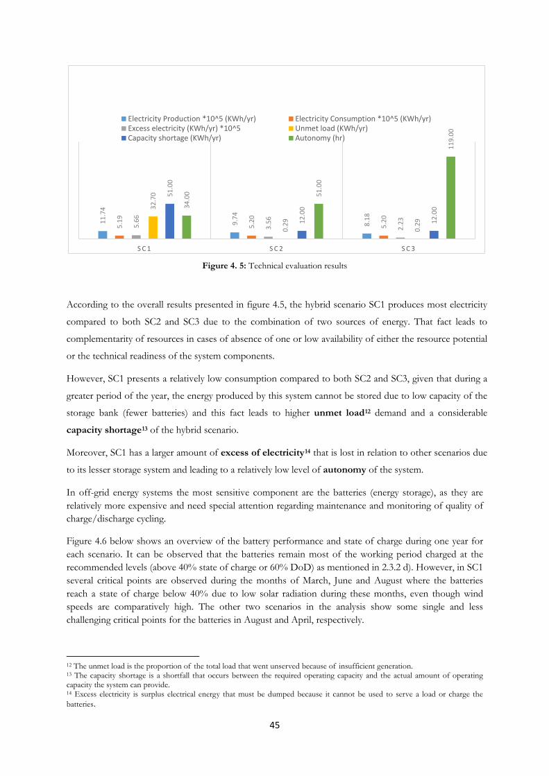
45
Figure 4. 5: Technical evaluation results
According to the overall results presented in figure 4.5, the hybrid scenario SC1 produces most electricity
compared to both SC2 and SC3 due to the combination of two sources of energy. That fact leads to
complementarity of resources in cases of absence of one or low availability of either the resource potential
or the technical readiness of the system components.
However, SC1 presents a relatively low consumption compared to both SC2 and SC3, given that during a
greater period of the year, the energy produced by this system cannot be stored due to low capacity of the
storage bank (fewer batteries) and this fact leads to higher unmet load12 demand and a considerable
capacity shortage13 of the hybrid scenario.
Moreover, SC1 has a larger amount of excess of electricity14 that is lost in relation to other scenarios due
to its lesser storage system and leading to a relatively low level of autonomy of the system.
In off-grid energy systems the most sensitive component are the batteries (energy storage), as they are relatively more expensive and need special attention regarding maintenance and monitoring of quality of charge/discharge cycling.
Figure 4.6 below shows an overview of the battery performance and state of charge during one year for each scenario. It can be observed that the batteries remain most of the working period charged at the recommended levels (above 40% state of charge or 60% DoD) as mentioned in 2.3.2 d). However, in SC1 several critical points are observed during the months of March, June and August where the batteries reach a state of charge below 40% due to low solar radiation during these months, even though wind speeds are comparatively high. The other two scenarios in the analysis show some single and less challenging critical points for the batteries in August and April, respectively.
12 The unmet load is the proportion of the total load that went unserved because of insufficient generation. 13 The capacity shortage is a shortfall that occurs between the required operating capacity and the actual amount of operating capacity the system can provide. 14 Excess electricity is surplus electrical energy that must be dumped because it cannot be used to serve a load or charge the batteries.
11.
74
9.7
4
8.1
8
5.1
9
5.2
0
5.2
0
5.6
6
3.5
6
2.2
3
32.
70
0.2
9
0.2
9
51.
00
12.
00
12.
00 34.
00
51.
00
119
.00
S C 1 S C 2 S C 3
Electricity Production *10^5 (KWh/yr) Electricity Consumption *10^5 (KWh/yr)Excess electricity (KWh/yr) *10^5 Unmet load (KWh/yr)Capacity shortage (KWh/yr) Autonomy (hr)

46
a)
b)
c) Figure 4. 6: Battery state of charge a) SC1; b) SC2; c) SC3
To overcome this problem, the installation of a remote control system to monitor the batteries’ state of charge has been suggested so that in case of dangerous DoD levels, the beneficiaries can be warned to reduce electricity usage by disconnecting some appliances that are not relevant in a specific point of time or totally switch off the electricity supply to the householders and leave only important infrastructures connected, such as schools, public lights, health centre, water pump etc, until the batteries are recharged.
Through the techno-economic analysis, it can be noted that although the SC1 have high values of excess electricity leading to electricity losses, most of the time the system is incapable to satisfy the load demand (unmet demand) and experiences more critical points of DoD compared to the other two scenarios, the SC1 remains the best option as it can meet the load at a relatively lowest cost.
Furthermore, the excess electricity produced by the SC1 system can be used in the future to connect more beneficiaries simply by adding more batteries and expanding the system boundaries, given that with the electrification of the village conditions will be created for enhanced local development and it is predicted that scattered people/householders will come closer seeking for electricity and availing of the related development possibilities.
If the demand continues increasing, the SC1 system remains feasible given the modularity of equipment structure. Or in other words, more batteries or more PV panels, wind turbines, etc, can be gradually added to increase electricity production successively.

47
5 CHAPTER FIVE: CONCLUSIONS AND RECOMMENDATIONS
5.1 Conclusions
The present work proposes the need for and performs a detailed feasibility study for implementing wind
and solar hybrid power system for rural electrification at the Estatuene Locality in the southern part of
Mozambique. The results of the assessment made on the availability of energy resources in the study area
show promising data for the implementation of the proposed system, as the annual average potential is
approximately 5.02 m/s for the wind velocity resource and 5.13 kWh/m2/day for the solar insolation
resource, respectively.
The feasibility analysis was attempted in order to find the most appropriate system for the electrification
of Estatuene combining the two energy sources (solar and wind) using the HOMER software. All system
scenarios need also to contain a large battery bank to cover the necessary demand.
The pre-evaluation considerations resulted in three optimal options/scenarios to be compared among
each-other in terms of performance and costs, namely:
• Solar-wind hybrid energy system,
• Solar PV energy system alone, and
• Wind turbine energy system alone.
However, once a critical analysis was made between these options it was concluded that the hybrid
combination appears to be more technically and economically feasible, because the costs of electricity
production using this system are lowest (0.34 $/kWh) compared to the other two options (0.37 $/kWh
for solar-only and 0.82 $/kWh for wind-only) and also involves less equipment especially in terms of
energy storage devices (battery charge).
Despite the fact that the levelized cost of electricity for the hybrid system is lower, it is still an unbearably
high investment for the economic capacity of rural communities in Mozambique, since even in urban
areas that are covered by the national grid (supplied by EDM), the cost of electricity for domestic use is
about 0.1 $USD/kWh. However, it is the government responsibility to supply electricity to citizens. So
for this kind of projects, the Government of Mozambique and cooperating partners provide funds for
implementation of rural electrification projects through FUNAE, and then it is up to the involved
communities to contribute about 15 USD/Month/beneficiary and ensure the necessary local maintenance
and operation-supporting procedures to keep the system properly running and to sustain the longevity of
the equipment.
In Mozambique the measures for rural electrification funded by the Government through FUNAE are
the implementation of small renewable energy systems, especially using PVs, but this technology has been

48
costly and technically impractical because these systems, in certain periods of the day or month, do not
support the load demand due to insufficient availability of the resource, in turn requiring a prohibitively
large energy storage auxiliary systems which further raise the costs. This situation could be overcome
through the implementation of hybrid (wind-solar) power systems.
5.2 Recommendations and future work
It is recommended that:
• Studies of this nature be transferred and implemented also in other parts of the country, to
determine the feasibility for implementation of hybrid projects using renewables elsewhere in
Mozambique; and
• The Estatuene project should be implemented in a pilot phase, so that later on it can be
replicated to other regions of the country that yet have not been covered by the national grid
authority EDM;
• Future socio-economic analysis must be made to evaluate the possibility so that the rural
communities should pay the regular EDM electricity tariff (0.1 USD/kWh) and the remaining
production cost (LCOE) inferred by renewable energy generation should be subsidized by the
Government.

49
LITERATURE
1. Ackermann, T. and Soder, L. 2000. Wind Energy Technology and Current Status: a Review. April 25, 2000.
2. Ahmed, S. 2011. Wind Energy. Theory and Practice. New Delhi-110001 : Asoke K. Ghosh, PHI Learning Private Limited M-97, 2011.
3. aliexpress. 2014. Aliexpress. Aliexpress. [Online] June 12, 2014. http://www.aliexpress.com/item/Supply-Wind-Turbine-10000W-High-quality-and-efficiency/377393099.html.
4. AWEA. 2014. AWEA. American Wind Energy Association . [Online] june 12, 2014. http://www.awea.org/Resources/Content.aspx?ItemNumber=5547.
5. BCS. 2014. Blue CHip Energy Solutions PTY Ltda. [Online] August 17, 2014. http://www.indiamart.com/bluechipenergysolutions/renewable-energy-products.html.
6. Burton, T., et al. 2011. Wind Energy Hand Book. Chichester, UK : John Wiley & Sons, Ltd, 2011.
7. Chen, C. J. 2011. Physics of Solar Energy. New Jersey - USA : John Wiley & Sons, Inc, 2011.
8. Coalition, The Wind. 2013. The Wind Coalition. The Wind Coalition. [Online] December 12, 2013. [Cited: September 13, 2013.] http://windcoalition.org/wind-energy/history-of-wind-energy/.
9. Cuamba, B. C., et al. 2006. A solar energy resources assessment in Mozambique. Cape Town : Journal of Energy in Southern Africa • Vol 17 No 4, 2006. p. 10.
10. Electronica. 2014. Electronica. [Online] March 11, 2014. http://www.electronica-pt.com/energia-solar/painel-solar-fotovoltaico/.
11. Enviroware. 2014. Enviroware. Enviroware. [Online] June 14, 2014. http://www.enviroware.com/METAR/METAR_WindRoses_2013_maps.html.
12. FUNAE. 2014. ATLAS - Renewable Energy of Mozambique. ATLAS - Renewable Energy of Mozambique. [Online] 8 16, 2014. http://www.atlasrenovaveis.co.mz/en.
13. Gipe, P. 2004. Wind Power. London : James & James (Science Publishers) Ltd, 2004. pp. 30-46; 50-67; 400-403.
14. Haberlin, H. 2012. Photovoltaics System Design and Practice. UK : John Wiley & Sons Ltd, 2012.
15. Hankins, M. 2009. A Renewable Energy Plan for Mozambique. Maputo-Mozambique : Justica Ambiental (JA), 2009.
16. Hankins, M. 2010. Stand-Alone Solar Electric System. Washington, DC : Earthscan, 2010.
17. INE. 2007. Recenceamento da Populacao. Maputo-Mozambique : Mozambique National Institute of Statistics -INE, 2007.
18. IOWA. 2013. IOWA Energy Center . IOWA Energy Center . [Online] September 10, 2013. [Cited: September 10, 2013.] http://www.energy.iastate.edu/renewable/wind/wem-index.html.
19. Johnson, G. L. 2006. Wind Energy System-Electronic Edition. Manhattan, KS : s.n., 2006.
20. Kalogirou, S. A. 2009. Solar Energy Engineering: Process and Systems. California, USA : Elsever, 2009.
21. LEM. 2014. LEM. LEM. [Online] February 26, 2014. http://lem.ch.unito.it/didattica/infochimica/2006_Complessi%20dipiridilici%20del%20rutenio/silicio.html.

50
22. Lenardic, Denis. 2014. EU PVSEC2014. EU PVSEC2014. [Online] June 12, 2014. http://www.pvresources.com/Economics/Investment.aspx.
23. Luque, A. and Hegeus, S. 2011. Handbook of Photovoltaic Science and Engineering, SecondEdition. Indiana, USA : John Willey & Sons, 2011.
24. Maini, A. K. and Agrawal, V. 2011. Satellite Technology: Principles and Applications, 2nd Edition. s.l. : Wiley, 2011.
25. Manwell, J., McGowan, J. and Rogers, A. 2009. wind energy Explained: Theory, Design and Application, Second Edition. UK : John Wiley & Sons, Ltd, 2009.
26. Mathew, S. and Philip, G. S. 2011. Advances in Wind Energy Conversion Technology. Verlag Berlin Heidelberg : Springer, 2011.
27. NREL. 2014. NREL. NREL. [Online] June 12, 2014. http://www.nrel.gov/news/press/2013/5306.html.
28. PALSOLAR. 2014. PAL SOLAR Mechanics & Energy Solutions. [Online] 03 08, 2014. http://www.palsolar.com/index.php/our-products/batteries.
29. Pazmino, V. 2007. PV-WInd Energy Systems Techno-Economic Feasibility, Analysis for Different Swedish Location. Hogskolan Dalarna Borlange : Hogskolan Dalarna Borlange, 2007.
30. PracticalAction. 2014. Practical Action. Practical Action. [Online] June 14, 2014. http://www.sswm.info/sites/default/files/reference_attachments/MAUPOUX%202010%20Solar%20Water%20Pumping.pdf.
31. Rageb, M. and Ragheb, A. M. 2011. Wind Turbines Theory - The Betz Equation and Optimal Rotor Tip Speed Ratio, Fundamental and Advanced Topics in Wind power. USA : InTech, 2011.
32. Rohatgi, J. S. and Nelson , V. 1994. Wind Characteristics - An Analysis for the Generation of wind power. USA : Alternative Energy Institute - West Texas A&M University, 1994.
33. SEI, Solar Energy International. 2004. Photovoltaics Design and Installation Manual. Canada : New Society Publishers, 2004.
34. Seraphim, O. J., et al. 2004. Eficiência Energética de Módulos Fotovoltaicos Mono e Poli-Cristalinos em Função da Radiação Solar Global. 2004.
35. Spera, D. A. 2009. Wind Turbine Technology. Fundamental Concepts of Wind Turbine Engineering. Second Edition. New York : ASME PRESS, 2009.
36. Stapleton, G. and Neill, S. 2012. Grid Connected Solar Electric System. New York, USA and Canada : Earthscan, 2012.
37. TheNoise. 2007. en.wikipedia. en.wikipedia. [Online] 08 04, 2007. [Cited: 10 08, 2013.] http://commons.wikimedia.org/wiki/File:Pn-junction-equilibrium.png.
38. Twidell, T and Weir, J. 2006. Renewable Resources. Second Edition. s.l. : Taylor & Francis Group, 2006. pp. 2-25; 263-319.
39. UNICAMP. 2014. http://www.ccs.unicamp.br/novosite/. http://www.ccs.unicamp.br/novosite/. [Online] 06 26, 2014. www.ccs.unicamp.br/cursos/ee941/download/cap04.pdf.
40. Walker, J. F. and Jenkins, N. 1997. Wind Energy Technology. England : John Wiley & Sons, 1997.
41. Wikpedia. 2014. Wikipedia. Wikipedia. [Online] February 27, 2014. http://en.wikipedia.org/wiki/Theory_of_solar_cells.
42. Wortman, A. J. 1983. Introduction to Wind Turbine Engineering. Woburn, MA 01801 Boston, U.S.A : Butterworth Publishers, 1983. pp. (Chp1) 1-5, (Chp2) 7-12, (Chp3) 3-5.

51
43. Yu, P. and Cardona, M. 2010. Fundamental of Semiconductors - Physics and Material Properties. 4th Edittion. s.l. : Spriger Editors., 2010.
44. Zucule, J. 2012. An Evaluation of Wind Energy Potential for Power Generation in Mozambique. Durban, SA : University of Kwazulu Natal, 2012.

52
APPENDICES
Appendix 1: FUNAE 4kW mini PV systems & typical electrified infrastructures/households.
Appendix 2: FUNAE Solar modules Characteristics
Technical Specifications Power (W) 150 Vmpp (V) 17.14 Impp (A) 8.17 Vca (V) 22.14 Isc (A) 8.69 Tolerance (%) 2.5 Vmax (V) 1000.0 Efficiency (%) 16.60

53
Appendix 3: Wind Turbines - FD6.4-5000 and FD8.0-10000 Characteristics
a) Technical Specifications
Parameter: FD6.4-5000 (DC) FD8.0-10000 (AC) Rated Power (W) 5000 10000 Rated Voltage (V) 240 240 Rotor diameter (m) 5.4 8 Start-up wind speed (m/s) 2 2.5 Rated wind speed (m/s) 12 16 Safety wind speed (m/s) 60 60 Rotating rate (r/m) 200 45 Blade material Fiber glass Reinforced fiber glass Blade quantity 3 3 Tower height (m) 12 12 Tower diameter (mm) 273 325 Matched inverter type Sine wave Sine wave (can choose 3 phase)
b) Wind Turbines’ power curves:

54
Appendix 4: 5000W off-grid, pure sine wave inverter, for solar and wind system.
Appendix 5: Batteries (2v, OPZS3500, 3000Ah)
Technical Specifications
Model Number OF5000 Type Pure sine wave off grid inverter Output Power (W) 5000
Input Voltage (v) 48/96
Output Current (A) 15 Output Voltage (V) 220/110 Output Frequency (Hz) 50/60

55
Appendix 6: Overall optimization results in HOMER
PV (kW)
FD 6.4
5000 FD8. 10000 H3000
Converter (kW)
Initial capital
Operating cost ($/yr)
Total NPC
COE ($/kWh)
Renewable fraction
Batt. Lf. (yr)
66 1 48 15 $185,783 3,198 $226,661 0.341 1 20
66.5 1 48 15 $186,428 3,204 $227,389 0.343 1 20
67 1 48 15 $187,072 3,211 $228,116 0.344 1 20
67.5 1 48 15 $187,717 3,217 $228,844 0.345 1 20
68 1 48 15 $188,361 3,224 $229,572 0.346 1 20
65 1 48 20 $187,424 3,388 $230,728 0.348 1 20
65.5 1 48 20 $188,069 3,394 $231,456 0.349 1 20
66 1 48 20 $188,713 3,401 $232,183 0.35 1 20
66.5 1 48 20 $189,358 3,407 $232,911 0.351 1 20
67 1 48 20 $190,002 3,414 $233,638 0.352 1 20
67.5 1 48 20 $190,647 3,420 $234,366 0.353 1 20
68 1 48 20 $191,291 3,427 $235,093 0.354 1 20
60 2 48 15 $194,176 3,281 $236,115 0.356 1 20
65 1 48 25 $190,354 3,590 $236,250 0.356 1 20
65.5 1 48 25 $190,999 3,597 $236,977 0.357 1 20
66 1 48 25 $191,643 3,603 $237,705 0.358 1 20
66.5 1 48 25 $192,288 3,610 $238,433 0.359 1 20
67 1 48 25 $192,932 3,616 $239,160 0.36 1 20
67.5 1 48 25 $193,577 3,623 $239,888 0.361 1 20
68 1 48 25 $194,221 3,629 $240,615 0.362 1 20
60 2 48 20 $197,106 3,484 $241,637 0.364 1 20
65 1 48 30 $193,284 3,793 $241,772 0.364 1 20
65.5 1 48 30 $193,929 3,800 $242,499 0.365 1 20
66 1 48 30 $194,573 3,806 $243,227 0.366 1 20
65 2 48 15 $200,621 3,346 $243,391 0.366 1 20
66.5 1 48 30 $195,218 3,813 $243,954 0.367 1 20
65.5 2 48 15 $201,266 3,352 $244,119 0.368 1 20
67 1 48 30 $195,862 3,819 $244,682 0.369 1 20
66 2 48 15 $201,910 3,359 $244,846 0.369 1 20
67.5 1 48 30 $196,507 3,826 $245,410 0.37 1 20
66.5 2 48 15 $202,555 3,365 $245,574 0.37 1 20
68 1 48 30 $197,151 3,832 $246,137 0.371 1 20
67 2 48 15 $203,199 3,372 $246,302 0.371 1 20
67.5 2 48 15 $203,844 3,378 $247,029 0.372 1 20
60 2 48 25 $200,036 3,686 $247,159 0.372 1 20
60 72 15 $199,818 3,744 $247,679 0.373 1 20
68 2 48 15 $204,488 3,385 $247,757 0.373 1 20
65 2 48 20 $203,551 3,549 $248,913 0.375 1 20
65.5 2 48 20 $204,196 3,555 $249,641 0.376 1 20
66 2 48 20 $204,840 3,562 $250,368 0.377 1 20
66.5 2 48 20 $205,485 3,568 $251,096 0.378 1 20

56
67 2 48 20 $206,129 3,575 $251,823 0.379 1 20
67.5 2 48 20 $206,774 3,581 $252,551 0.38 1 20
60 2 48 30 $202,966 3,889 $252,681 0.381 1 20
60 72 20 $202,748 3,947 $253,201 0.381 1 20
68 2 48 20 $207,418 3,588 $253,279 0.381 1 20
60 3 48 15 $210,303 3,442 $254,300 0.383 1 20
65 2 48 25 $206,481 3,751 $254,435 0.383 1 20
65 72 15 $206,263 3,809 $254,955 0.384 1 20
65.5 2 48 25 $207,126 3,758 $255,162 0.384 1 20
65.5 72 15 $206,908 3,816 $255,683 0.385 1 20
66 2 48 25 $207,770 3,764 $255,890 0.385 1 20
66 72 15 $207,552 3,822 $256,410 0.386 1 20
66.5 2 48 25 $208,415 3,771 $256,618 0.386 1 20
66.5 72 15 $208,197 3,829 $257,138 0.387 1 20
67 2 48 25 $209,059 3,777 $257,345 0.387 1 20
67 72 15 $208,841 3,835 $257,866 0.388 1 20
67.5 2 48 25 $209,704 3,784 $258,073 0.389 1 20
67.5 72 15 $209,486 3,842 $258,593 0.389 1 20
60 72 25 $205,678 4,150 $258,723 0.39 1 20
68 2 48 25 $210,348 3,790 $258,800 0.39 1 20
68 72 15 $210,130 3,848 $259,321 0.39 1 20
60 3 48 20 $213,233 3,645 $259,822 0.391 1 20
65 2 48 30 $209,411 3,954 $259,957 0.391 1 20
65 72 20 $209,193 4,012 $260,477 0.392 1 20
65.5 2 48 30 $210,056 3,961 $260,684 0.392 1 20
65.5 72 20 $209,838 4,018 $261,205 0.393 1 20
66 2 48 30 $210,700 3,967 $261,412 0.394 1 20
65 3 48 15 $216,748 3,507 $261,576 0.394 1 20
66 72 20 $210,482 4,025 $261,932 0.394 1 20
66.5 2 48 30 $211,345 3,974 $262,140 0.395 1 20
65.5 3 48 15 $217,393 3,513 $262,304 0.395 1 20
66.5 72 20 $211,127 4,031 $262,660 0.395 1 20
67 2 48 30 $211,989 3,980 $262,867 0.396 1 20
66 3 48 15 $218,037 3,520 $263,032 0.396 1 20
67 72 20 $211,771 4,038 $263,387 0.397 1 20
67.5 2 48 30 $212,634 3,987 $263,595 0.397 1 20
66.5 3 48 15 $218,682 3,526 $263,759 0.397 1 20
67.5 72 20 $212,416 4,044 $264,115 0.398 1 20
60 72 30 $208,608 4,352 $264,245 0.398 1 20
68 2 48 30 $213,278 3,993 $264,322 0.398 1 20
67 3 48 15 $219,326 3,533 $264,487 0.398 1 20
68 72 20 $213,060 4,051 $264,843 0.399 1 20
67.5 3 48 15 $219,971 3,539 $265,214 0.399 1 20
60 3 48 25 $216,163 3,847 $265,344 0.399 1 20
60 1 72 15 $215,945 3,905 $265,864 0.4 1 20
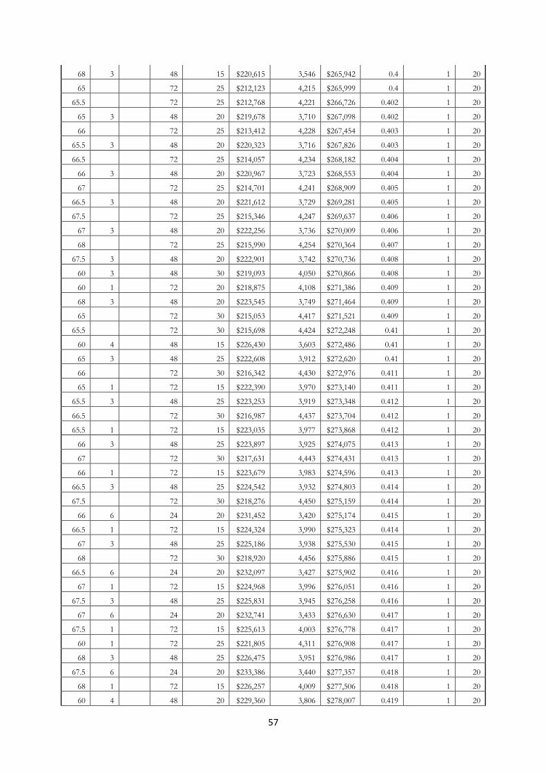
57
68 3 48 15 $220,615 3,546 $265,942 0.4 1 20
65 72 25 $212,123 4,215 $265,999 0.4 1 20
65.5 72 25 $212,768 4,221 $266,726 0.402 1 20
65 3 48 20 $219,678 3,710 $267,098 0.402 1 20
66 72 25 $213,412 4,228 $267,454 0.403 1 20
65.5 3 48 20 $220,323 3,716 $267,826 0.403 1 20
66.5 72 25 $214,057 4,234 $268,182 0.404 1 20
66 3 48 20 $220,967 3,723 $268,553 0.404 1 20
67 72 25 $214,701 4,241 $268,909 0.405 1 20
66.5 3 48 20 $221,612 3,729 $269,281 0.405 1 20
67.5 72 25 $215,346 4,247 $269,637 0.406 1 20
67 3 48 20 $222,256 3,736 $270,009 0.406 1 20
68 72 25 $215,990 4,254 $270,364 0.407 1 20
67.5 3 48 20 $222,901 3,742 $270,736 0.408 1 20
60 3 48 30 $219,093 4,050 $270,866 0.408 1 20
60 1 72 20 $218,875 4,108 $271,386 0.409 1 20
68 3 48 20 $223,545 3,749 $271,464 0.409 1 20
65 72 30 $215,053 4,417 $271,521 0.409 1 20
65.5 72 30 $215,698 4,424 $272,248 0.41 1 20
60 4 48 15 $226,430 3,603 $272,486 0.41 1 20
65 3 48 25 $222,608 3,912 $272,620 0.41 1 20
66 72 30 $216,342 4,430 $272,976 0.411 1 20
65 1 72 15 $222,390 3,970 $273,140 0.411 1 20
65.5 3 48 25 $223,253 3,919 $273,348 0.412 1 20
66.5 72 30 $216,987 4,437 $273,704 0.412 1 20
65.5 1 72 15 $223,035 3,977 $273,868 0.412 1 20
66 3 48 25 $223,897 3,925 $274,075 0.413 1 20
67 72 30 $217,631 4,443 $274,431 0.413 1 20
66 1 72 15 $223,679 3,983 $274,596 0.413 1 20
66.5 3 48 25 $224,542 3,932 $274,803 0.414 1 20
67.5 72 30 $218,276 4,450 $275,159 0.414 1 20
66 6 24 20 $231,452 3,420 $275,174 0.415 1 20
66.5 1 72 15 $224,324 3,990 $275,323 0.414 1 20
67 3 48 25 $225,186 3,938 $275,530 0.415 1 20
68 72 30 $218,920 4,456 $275,886 0.415 1 20
66.5 6 24 20 $232,097 3,427 $275,902 0.416 1 20
67 1 72 15 $224,968 3,996 $276,051 0.416 1 20
67.5 3 48 25 $225,831 3,945 $276,258 0.416 1 20
67 6 24 20 $232,741 3,433 $276,630 0.417 1 20
67.5 1 72 15 $225,613 4,003 $276,778 0.417 1 20
60 1 72 25 $221,805 4,311 $276,908 0.417 1 20
68 3 48 25 $226,475 3,951 $276,986 0.417 1 20
67.5 6 24 20 $233,386 3,440 $277,357 0.418 1 20
68 1 72 15 $226,257 4,009 $277,506 0.418 1 20
60 4 48 20 $229,360 3,806 $278,007 0.419 1 20

58
68 6 24 20 $234,030 3,446 $278,085 0.419 1 20
65 3 48 30 $225,538 4,115 $278,142 0.419 1 20
65 1 72 20 $225,320 4,173 $278,662 0.42 1 20
65.5 3 48 30 $226,183 4,122 $278,869 0.42 1 20
60 7 24 15 $236,915 3,301 $279,107 0.42 1 20
65.5 1 72 20 $225,965 4,179 $279,390 0.421 1 20
66 3 48 30 $226,827 4,128 $279,597 0.421 1 20
65 4 48 15 $232,875 3,668 $279,761 0.421 1 20
65 2 48 15 $232,875 3,670 $279,787 0.422 1 20
66 1 72 20 $226,609 4,186 $280,117 0.422 1 20
66.5 3 48 30 $227,472 4,135 $280,325 0.422 1 20
65.5 4 48 15 $233,520 3,674 $280,489 0.422 1 20
65.5 2 48 15 $233,520 3,676 $280,515 0.423 1 20
66 6 24 25 $234,382 3,623 $280,696 0.423 1 20
66.5 1 72 20 $227,254 4,192 $280,845 0.423 1 20
67 3 48 30 $228,116 4,141 $281,052 0.423 1 20
66 4 48 15 $234,164 3,681 $281,217 0.423 1 20
66 2 48 15 $234,164 3,683 $281,242 0.424 1 20
66.5 6 24 25 $235,027 3,630 $281,424 0.424 1 20
67 1 72 20 $227,898 4,199 $281,573 0.424 1 20
67.5 3 48 30 $228,761 4,148 $281,780 0.424 1 20
66.5 4 48 15 $234,809 3,687 $281,944 0.424 1 20
66.5 2 48 15 $234,809 3,689 $281,970 0.425 1 20
67 6 24 25 $235,671 3,636 $282,151 0.425 1 20
67.5 1 72 20 $228,543 4,205 $282,300 0.425 1 20
60 1 72 30 $224,735 4,513 $282,430 0.425 1 20
68 3 48 30 $229,405 4,154 $282,507 0.425 1 20
67 4 48 15 $235,453 3,694 $282,672 0.426 1 20
67 2 48 15 $235,453 3,696 $282,697 0.426 1 20
67.5 6 24 25 $236,316 3,643 $282,879 0.426 1 20
68 1 72 20 $229,187 4,212 $283,028 0.426 1 20
67.5 4 48 15 $236,098 3,700 $283,399 0.427 1 20
67.5 2 48 15 $236,098 3,702 $283,425 0.427 1 20
60 4 48 25 $232,290 4,008 $283,529 0.427 1 20
68 6 24 25 $236,960 3,649 $283,607 0.427 1 20
60 2 72 15 $232,072 4,066 $284,050 0.428 1 20
60 1 72 15 $232,072 4,067 $284,062 0.428 1 20
68 4 48 15 $236,742 3,707 $284,127 0.428 1 20
68 2 48 15 $236,742 3,709 $284,153 0.428 1 20
65 1 72 25 $228,250 4,376 $284,184 0.428 1 20
60 7 24 20 $239,845 3,503 $284,628 0.429 1 20
65.5 1 72 25 $228,895 4,382 $284,912 0.429 1 20
65 4 48 20 $235,805 3,871 $285,283 0.429 1 20
65 2 48 20 $235,805 3,873 $285,309 0.43 1 20
66 1 72 25 $229,539 4,389 $285,639 0.43 1 20

59
65.5 4 48 20 $236,450 3,877 $286,011 0.431 1 20
65.5 2 48 20 $236,450 3,879 $286,036 0.431 1 20
66 6 24 30 $237,312 3,826 $286,218 0.431 1 20
66.5 1 72 25 $230,184 4,395 $286,367 0.431 1 20
65 7 24 15 $243,360 3,366 $286,383 0.431 1 20
66 4 48 20 $237,094 3,884 $286,738 0.432 1 20
66 2 48 20 $237,094 3,886 $286,764 0.432 1 20
66.5 6 24 30 $237,957 3,832 $286,946 0.432 1 20
67 1 72 25 $230,828 4,402 $287,094 0.432 1 20
65.5 7 24 15 $244,005 3,372 $287,110 0.432 1 20
66.5 4 48 20 $237,739 3,890 $287,466 0.433 1 20
66.5 2 48 20 $237,739 3,892 $287,492 0.433 1 20
67 6 24 30 $238,601 3,839 $287,673 0.433 1 20
67.5 1 72 25 $231,473 4,408 $287,822 0.433 1 20
66 7 24 15 $244,649 3,379 $287,838 0.433 1 20
67 4 48 20 $238,383 3,897 $288,194 0.434 1 20
67 2 48 20 $238,383 3,899 $288,219 0.434 1 20
67.5 6 24 30 $239,246 3,845 $288,401 0.434 1 20
68 1 72 25 $232,117 4,415 $288,550 0.434 1 20
66.5 7 24 15 $245,294 3,385 $288,565 0.435 1 20
67.5 4 48 20 $239,028 3,903 $288,921 0.435 1 20
67.5 2 48 20 $239,028 3,905 $288,947 0.435 1 20
60 4 48 30 $235,220 4,211 $289,051 0.435 1 20
68 6 24 30 $239,890 3,852 $289,129 0.436 1 20

60
Appendix 7: Scenario 1, 2 and 3 System Report SC1 – System Report Sensitivity case Solar Data Scaled Average: 5.13 kWh/m²/d
Wind Data Scaled Average: 5.02 m/s
WT FD8.0-10000 --10KW Hub Height: 12 m
System architecture PV Array 66 kW Wind turbine 1 FD6.4-5000-16 Battery 48 Hoppecke 24 OPzS 3000 Inverter 15 kW Rectifier 15 kW Cost summary Total net present cost $ 226,661
Levelized cost of energy $ 0.341/kWh
Operating cost $ 3,198/yr
Net Present Costs
Component Capital Replacement O&M Fuel Salvage Total
($) ($) ($) ($) ($) ($)
PV 85,074 0 10,968 0 0 96,042
FD6.4-5000-16 16,127 0 2,058 0 0 18,185
Hoppecke 24 OPzS 3000 75,792 23,632 9,689 0 -13,245 95,868
Converter 8,790 7,649 1,151 0 -1,024 16,566
System 185,783 31,281 23,866 0 -14,269 226,661

61
Annualized Costs
Component Capital Replacement O&M Fuel Salvage Total
($/yr) ($/yr) ($/yr) ($/yr) ($/yr) ($/yr)
PV 6,655 0 858 0 0 7,513
FD6.4-5000-16 1,262 0 161 0 0 1,423
Hoppecke 24 OPzS 3000 5,929 1,849 758 0 -1,036 7,499
Converter 688 598 90 0 -80 1,296
System 14,533 2,447 1,867 0 -1,116 17,731
Electrical
Load Consumption Fraction
(kWh/yr)
AC primary load 48,513 93%
DC primary load 3,416 7%
Total 51,929 100%
Component Production Fraction
(kWh/yr)
PV array 107,193 91%
Wind turbine 10,231 9%
Total 117,424 100%
Quantity Value Units
Excess electricity 56,559 kWh/yr
Unmet load 32.4 kWh/yr
Capacity shortage 50.4 kWh/yr
Renewable fraction 1.000
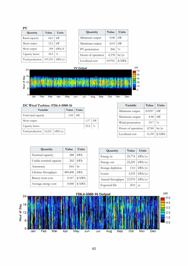
62
PV
Quantity Value Units
Rated capacity 66.0 kW
Mean output 12.2 kW
Mean output 294 kWh/d
Capacity factor 18.5 %
Total production 107,193 kWh/yr
DC Wind Turbine: FD6.4-5000-16
Variable Value Units
Total rated capacity 5.00 kW
Mean output 1.17 kW
Capacity factor 23.4 %
Total production 10,231 kWh/yr
Quantity Value Units
Minimum output 0.00 kW
Maximum output 63.9 kW
PV penetration 206 %
Hours of operation 4,378 hr/yr
Levelized cost 0.0701 $/kWh
Variable Value Units
Minimum output 0.0357 kW
Maximum output 4.98 kW
Wind penetration 19.7 %
Hours of operation 8,760 hr/yr
Levelized cost 0.139 $/kWh
Quantity Value Units
Nominal capacity 288 kWh
Usable nominal capacity 202 kWh
Autonomy 34.0 hr
Lifetime throughput 489,408 kWh
Battery wear cost 0.167 $/kWh
Average energy cost 0.000 $/kWh
Quantity Value Units
Energy in 25,774 kWh/yr
Energy out 22,229 kWh/yr
Storage depletion 13.0 kWh/yr
Losses 3,533 kWh/yr
Annual throughput 23,970 kWh/yr
Expected life 20.0 yr
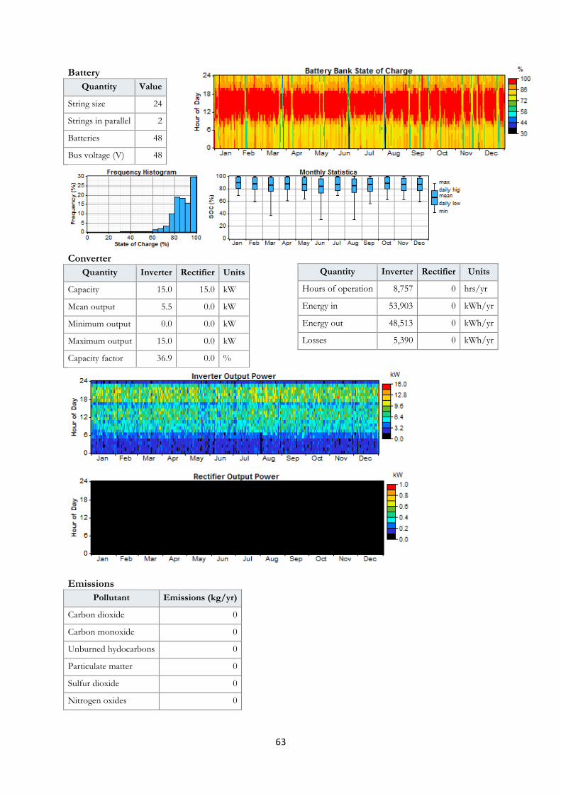
63
Battery Quantity Value
String size 24
Strings in parallel 2
Batteries 48
Bus voltage (V) 48
Converter
Quantity Inverter Rectifier Units
Capacity 15.0 15.0 kW
Mean output 5.5 0.0 kW
Minimum output 0.0 0.0 kW
Maximum output 15.0 0.0 kW
Capacity factor 36.9 0.0 %
Emissions
Pollutant Emissions (kg/yr)
Carbon dioxide 0
Carbon monoxide 0
Unburned hydocarbons 0
Particulate matter 0
Sulfur dioxide 0
Nitrogen oxides 0
Quantity Inverter Rectifier Units
Hours of operation 8,757 0 hrs/yr
Energy in 53,903 0 kWh/yr
Energy out 48,513 0 kWh/yr
Losses 5,390 0 kWh/yr

64
SC2 – System Report Sensitivity case Solar Data Scaled Average: 5.13 kWh/m²/d
Wind Data Scaled Average: 5.02 m/s
WT FD8.0-10000 --10KW Hub Height: 12 m
System architecture PV Array 60 kW Battery 72 Hoppecke 24 OPzS 3000 Inverter 15 kW Rectifier 15 kW
Cost summary
Total net present cost $ 247,679
Levelized cost of energy $ 0.373/kWh
Operating cost $ 3,744/yr
Net Present Costs
Component Capital Replacement O&M Fuel Salvage Total
($) ($) ($) ($) ($) ($)
PV 77,340 0 9,971 0 0 87,311
Hoppecke 24 OPzS 3000 113,688 35,448 14,533 0 -19,867 143,803
Converter 8,790 7,649 1,151 0 -1,024 16,566
System 199,818 43,098 25,655 0 -20,891 247,679
Annualized Costs
Component Capital Replacement O&M Fuel Salvage Total
($/yr) ($/yr) ($/yr) ($/yr) ($/yr) ($/yr)
PV 6,050 0 780 0 0 6,830
Hoppecke 24 OPzS 3000 8,893 2,773 1,137 0 -1,554 11,249
Converter 688 598 90 0 -80 1,296
System 15,631 3,371 2,007 0 -1,634 19,375

65
Electrical
Load Consumption Fraction
(kWh/yr)
AC primary load 48,545 93%
DC primary load 3,416 7%
Total 51,961 100%
PV
Quantity Value Units
Rated capacity 60.0 kW
Mean output 11.1 kW
Mean output 267 kWh/d
Capacity factor 18.5 %
Total production 97,448 kWh/yr
Component Production Fraction
(kWh/yr)
PV array 97,448 100%
Total 97,448 100%
Quantity Value Units
Excess electricity 35,628 kWh/yr
Unmet load 0.291 kWh/yr
Capacity shortage 12.0 kWh/yr
Renewable fraction 1.000
Quantity Value Units
Minimum output 0.00 kW
Maximum output 58.1 kW
PV penetration 188 %
Hours of operation 4,378 hr/yr
Levelized cost 0.0701 $/kWh

66
Battery
Converter
Quantity Inverter Rectifier Units
Capacity 15.0 15.0 kW
Mean output 5.5 0.0 kW
Minimum output 0.0 0.0 kW
Maximum output 15.0 0.0 kW
Capacity factor 36.9 0.0 %
Emissions
Pollutant Emissions (kg/yr)
Carbon dioxide 0
Carbon monoxide 0
Unburned hydocarbons 0
Particulate matter 0
Sulfur dioxide 0
Nitrogen oxides 0
Quantity Value Units
Energy in 32,728 kWh/yr
Energy out 28,262 kWh/yr
Storage depletion 43.3 kWh/yr
Losses 4,422 kWh/yr
Annual throughput 30,476 kWh/yr
Expected life 20.0 yr
Quantity Value Units
Nominal capacity 432 kWh
Usable nominal capacity 302 kWh
Autonomy 51.0 hr
Lifetime throughput 734,112 kWh
Battery wear cost 0.167 $/kWh
Average energy cost 0.000 $/kWh
Quantity Value
String size 24
Strings in parallel 3
Batteries 72
Bus voltage (V) 48
Quantity Inverter Rectifier Units
Hours of operation 8,759 0 hrs/yr
Energy in 53,939 0 kWh/yr
Energy out 48,545 0 kWh/yr
Losses 5,394 0 kWh/yr

67
SC3 – System Report Sensitivity case Solar Data Scaled Average: 5.13 kWh/m²/d Wind Data Scaled Average: 5.02 m/s WT FD8.0-10000 --10KW Hub Height: 12 m System architecture Wind turbine 8 FD6.4-5000-16 Battery 192 Hoppecke 24 OPzS 3000 Inverter 15 kW Rectifier 15 kW Cost summary Total net present cost $ 545,520
Levelized cost of energy $ 0.821/kWh
Operating cost $ 8,178/yr
Net Present Costs
Component Capital Replacement O&M Fuel Salvage Total
($) ($) ($) ($) ($) ($)
FD6.4-5000-16 129,016 0 16,465 0 0 145,481
Hoppecke 24 OPzS 3000 303,168 94,529 38,755 0 -52,978 383,474
Converter 8,790 7,649 1,151 0 -1,024 16,566
System 440,974 102,178 56,371 0 -54,002 545,520
Annualized Costs
Component Capital Replacement O&M Fuel Salvage Total
($/yr) ($/yr) ($/yr) ($/yr) ($/yr) ($/yr)
FD6.4-5000-16 10,092 0 1,288 0 0 11,380
Hoppecke 24 OPzS 3000 23,716 7,395 3,032 0 -4,144 29,998
Converter 688 598 90 0 -80 1,296
System 34,496 7,993 4,410 0 -4,224 42,674
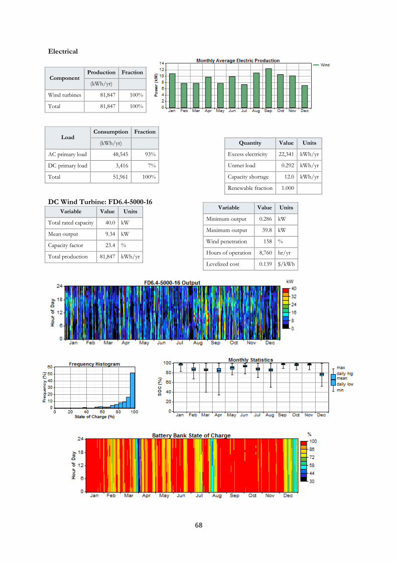
68
Electrical
DC Wind Turbine: FD6.4-5000-16
Variable Value Units
Total rated capacity 40.0 kW
Mean output 9.34 kW
Capacity factor 23.4 %
Total production 81,847 kWh/yr
Component Production Fraction
(kWh/yr)
Wind turbines 81,847 100%
Total 81,847 100%
Load Consumption Fraction
(kWh/yr)
AC primary load 48,545 93%
DC primary load 3,416 7%
Total 51,961 100%
Quantity Value Units
Excess electricity 22,341 kWh/yr
Unmet load 0.292 kWh/yr
Capacity shortage 12.0 kWh/yr
Renewable fraction 1.000
Variable Value Units
Minimum output 0.286 kW
Maximum output 39.8 kW
Wind penetration 158 %
Hours of operation 8,760 hr/yr
Levelized cost 0.139 $/kWh

69
Battery Quantity Value
String size 24
Strings in parallel 8
Batteries 192
Bus voltage (V) 48
Converter Quantity Inverter Rectifier Units
Capacity 15.0 15.0 kW
Mean output 5.5 0.0 kW
Minimum output 0.0 0.0 kW
Maximum output 15.0 0.0 kW
Capacity factor 36.9 0.0 %
Emissions
Pollutant Emissions (kg/yr)
Carbon dioxide 0
Carbon monoxide 0
Unburned hydocarbons 0
Particulate matter 0
Sulfur dioxide 0
Nitrogen oxides 0
Quantity Value Units
Energy in 16,846 kWh/yr
Energy out 14,696 kWh/yr
Storage depletion 5.35 kWh/yr
Losses 2,145 kWh/yr
Annual throughput 15,847 kWh/yr
Expected life 20.0 yr
Quantity Value Units
Nominal capacity 1,152 kWh
Usable nominal capacity 806 kWh
Autonomy 136 hr
Lifetime throughput 1,957,632 kWh
Battery wear cost 0.167 $/kWh
Average energy cost 0.000 $/kWh
Quantity Inverter Rectifier Units
Hours of operation 8,759 0 hrs/yr
Energy in 53,939 0 kWh/yr
Energy out 48,545 0 kWh/yr
Losses 5,394 0 kWh/yr