FDI as an Outcome of the Market forCorporate Control: Theory and Evidence∗

Keith Head† John Ries‡

April 3, 2007

Abstract

Much foreign direct investment (FDI) takes the form of mergers and acquisitions

(M&A). It is commonplace in finance to view acquisitions as manifestations of the market

for corporate control. Following on that insight we propose a model of FDI in which

headquarters bid to control overseas assets. We derive an equation for bilateral FDI

stocks that resembles the recently developed fixed effects approach to modelling bilateral

trade flows. We estimate the model and use its parameters to construct benchmarks for

evaluating multilateral inward and outward FDI.

JEL classification: F21, F22, G34

Keywords: foreign direct investment, mergers and acquisitions, gravity, benchmark

∗We appreciate the helpful suggestions of two anonymous referees, Jonathan Eaton, and workshop partic-ipants at the London School of Economics, CEPII and EIIT. We thank Thierry Mayer for providing some ofthe data used in this paper.

†Sauder School of Business, University of British Columbia, keith.head@ubc.ca‡Corresponding Author: Sauder School of Business, University of British Columbia, 2053 Main Mall,

Vancouver, BC, V6T1Z2, Canada. Tel: (604) 822-8493, Fax: (604) 822-8477, john.ries@ubc.ca

1 Introduction

From 1987 to 2001, about two-thirds of foreign direct investment (FDI) took the form of

mergers and acquisitions (M&A) rather than new plants. While it often makes sense to think

of M&A and greenfield investments as alternatives in a “buy or build” decision, this need not

be the primary consideration. For example, when Renault took a one third share of Nissan,

it had not been contemplating building a Renault factory in Japan. There was no intention

of shifting production of Renault models to Japanese factories. Instead, Renault installed

one of its star managers, Carlos Ghosn, as the Nissan CEO. He proceeded to restructure the

Japanese company, restoring it to profitability. This case illustrates the way that FDI can be

a manifestation of an international market for corporate control.

This paper develops a simple model of FDI where heterogeneous investors bid to obtain

control rights on existing overseas assets. Unlike much of the existing theoretical literature

predicting FDI, our formulation explicitly considers more than two countries. The model

yields an equation for bilateral FDI that strongly resembles the gravity equation used to

analyze bilateral trade in goods. The specification consists of an outward effect reflecting

characteristics of the origin country, an inward effect reflecting characteristics of the destina-

tion country, and a vector of pair-specific variables reflecting monitoring costs. We estimate

the model using a cross-section of 62 countries. In a second stage, we relate the estimated

inward and outward fixed effects to variables predicted by the model. We then show how a

formulation of the model can be aggregated to yield a simple expression for a country’s share

of world FDI. We compare predicted country-level inward and outward FDI shares to actual

values to see how well the model fits multilateral data and identify countries with anomalous

FDI performance.

The theoretical FDI literature has traditionally focussed on greenfield investment. Impor-

tant early work includes Markusen’s (1984) model of horizontal FDI and Helpman’s (1984)

model of vertical FDI. Carr, Markusen, and Maskus (2001) solve a 47-equation, general equi-

librium model incorporating vertical and horizontal FDI. Their computations suggest linear

1

FDI equations where key variables enter with interactions to capture non-linearities in the

model. Bergstrand and Egger (2004) add physical capital to Markusen’s knowledge-capital

model. They generate “theoretical flow data” and find the “frictionless” (no trade costs)

gravity equation describes their simulated data well.

A smaller, but growing, literature considers FDI in the form of cross-border M&A. Barba

Navaretti and Venables (2004) distinguish M&A from greenfield by assuming that merged

firms eliminate one of the varieties and the associated fixed costs of the joining firms. In

common with horizontal greenfield investment, cross-border M&A becomes more attractive

relative to exporting as trade costs increase. Neary (2004) also focuses on the market structure

implications of M&A but explores the implications of cost asymmetries between acquiring and

target firms. In his model low cost firms from one country acquire—and then shut down—high

cost firms abroad. Nocke and Yeaple (2005a) posit M&A as providing access to a foreign firm’s

non-mobile capabilities. Firms choose different modes of foreign entry (export, greenfield

and M&A) depending on their heterogeneous capabilities. Nocke and Yeaple (2005b) model

international acquisitions as arising from a matching between heterogeneous entrepreneurs

and varieties. All of these models abstract from one the main considerations of our paper:

the frictions that inhibit cross-border ownership.

One natural way to model frictions affecting FDI is to assume that headquarters have

imperfect information regarding assets in potential host countries. This approach has some

precedents in the international finance literature. Gordon and Bovenberg (1996) stipulate that

international buyers have a lower opportunity cost of capital but face information asymmetries

when they purchase domestic firms. In Razin and Goldstein (2005) and Razin, Sadka, and

Yuen (1998), foreign direct investors have informational advantages over portfolio investors.

Mody, Razin and Sadka (2004) and Loungani, Mody, Razin and Sadka (2003) propose that

foreign investors have specialized knowledge that gives them an advantage over domestic

owners. However, that advantage declines with greater corporate transparency in the host

country. None of the papers associate information problems with geography. One paper that

explicitly considers monitoring costs that are a function of distance is Marin and Schnitzer

2

(2004). That paper constructs and estimates a model of the headquarters decision to use its

own funds to finance direct investment (internal financing) or to rely upon loans from local

or international banks.

This paper’s contribution to the theory literature comes through an explicit model of

monitoring in which we establish an ability versus proximity tradeoff. We build this into a

highly stylized international market for corporate control. In our model, a country’s likelihood

of bidding successfully for assets in another country depends not only on the distance between

the two countries, but also their location relative to bidders in other countries. This approach

allows us to incorporate geography into an analytical expression for bilateral FDI in a multi-

country world. Our model provides a set of micro-foundations for a gravity equation for FDI.

Other models may provide a different set of micro-foundations for the same equation.1 Our

purpose is not to test our model against possible alternatives. Rather, we offer an analytical

structure on which to base estimation of bilateral FDI.

A growing empirical literature uses the gravity equation to investigate the determinants of

various types of cross-border investments. The base gravity equation relates the log of bilateral

investment to the logged sizes of origin and destination economies and the log distance between

them. Studies on FDI have then augmented the gravity equation with variables such as factor

endowments (Eaton and Tamura, 1994), corruption and taxes (Wei, 2000), third-country

competition (Eichengreen and Tong, 2005), information proxies (Loungani et al., 2003), taxes

and wages (Mutti and Grubert, 2004), and institutions (Benassy-Quere et al. 2007). Hijzen,

Gorg, and Manchin (2005) and di Giovanni (2005) investigate the determinants of bilateral

M&A transactions in a gravity setting. Portes and Rey (2005) find that gravity models also

fit portfolio investment flows.

Policy is often most interested in total FDI rather than geographic origins. Our multilat-

eral benchmarks contribute to the identification of unusually high or low FDI performance.

1Martin and Rey (2004) derive a gravity-type model for foreign portfolio investment assuming risk adverseinvestors and iceberg transaction costs for assets. Models of horizontal FDI predict that distance costs oftrade would promote investment. However, if final goods were non-traded but required inputs from home,high trade costs could lead to the negative distance effect exhibited in the gravity equation (see Grossman,Helpman, and Szeidl, 2003, for a model that admits this possibility).

3

The United Nations Conference on Trade and Development’s (UNCTAD) “FDI Performance

Index” compares countries’ shares of world FDI to shares of world GDP. Our theory identifies

biases in the UNCTAD index and our empirical implementation shows that our benchmark

generally achieves a tighter fit with actual FDI.

The next section presents the model and the corresponding specifications of bilateral and

multilateral FDI. Section 3 describes OECD and UNCTAD data on FDI and M&A. Here we

argue that a model of FDI as a market for corporate control may represent a large share of

FDI. Section 4 describes the results for bilateral FDI and M&A. We proceed in two stages.

In the first stage, we use bilateral FDI for 62 OECD and partner countries to estimate origin

and destination fixed effects. In the second stage, we estimate the unknown model parameters

and investigate the empirical validity of the model’s predictions. Section 5 uses the estimated

parameters to predict country-level aggregate foreign investment for 172 countries. Then

we compare the predictions to actual country-level shares of FDI & cross-border M&A. We

summarize our methods and results in the final section.

2 The model

We develop a control-based model of FDI. Jensen and Ruback (1983) motivate this approach,

arguing that “the market for corporate control is best viewed as an arena in which managerial

teams compete for the rights to manage corporate resources.” The model proceeds in three

subsections. First, we specify the costs and benefits of controlling remote assets in a game

between the headquarters of an MNE and a subsidiary. Second, we use discrete choice theory

to solve for the expected amount of corporate assets in one country that will be controlled

by a management team based in another country. This yields an expression for bilateral FDI

stocks. Third, we specify the predictions of our model for a country’s multilateral inward and

outward FDI.

4

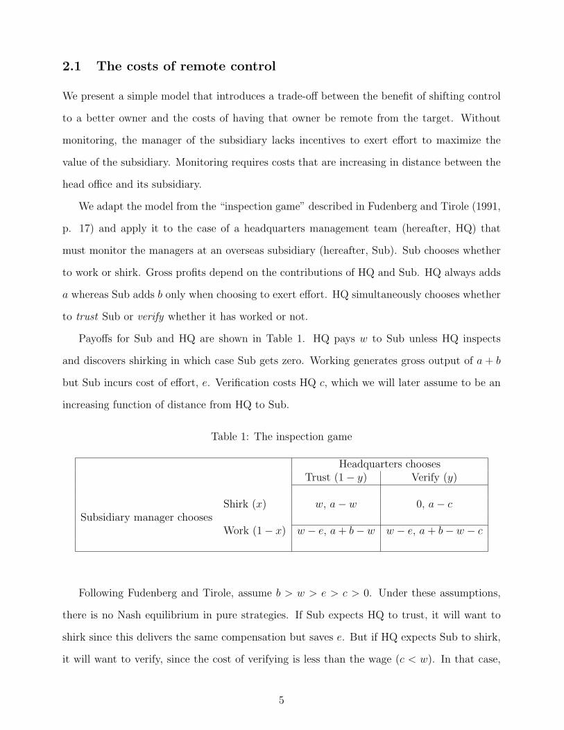
2.1 The costs of remote control

We present a simple model that introduces a trade-off between the benefit of shifting control

to a better owner and the costs of having that owner be remote from the target. Without

monitoring, the manager of the subsidiary lacks incentives to exert effort to maximize the

value of the subsidiary. Monitoring requires costs that are increasing in distance between the

head office and its subsidiary.

We adapt the model from the “inspection game” described in Fudenberg and Tirole (1991,

p. 17) and apply it to the case of a headquarters management team (hereafter, HQ) that

must monitor the managers at an overseas subsidiary (hereafter, Sub). Sub chooses whether

to work or shirk. Gross profits depend on the contributions of HQ and Sub. HQ always adds

a whereas Sub adds b only when choosing to exert effort. HQ simultaneously chooses whether

to trust Sub or verify whether it has worked or not.

Payoffs for Sub and HQ are shown in Table 1. HQ pays w to Sub unless HQ inspects

and discovers shirking in which case Sub gets zero. Working generates gross output of a + b

but Sub incurs cost of effort, e. Verification costs HQ c, which we will later assume to be an

increasing function of distance from HQ to Sub.

Table 1: The inspection game

Headquarters choosesTrust (1− y) Verify (y)

Shirk (x) w, a− w 0, a− cSubsidiary manager chooses

Work (1− x) w − e, a + b− w w − e, a + b− w − c

Following Fudenberg and Tirole, assume b > w > e > c > 0. Under these assumptions,

there is no Nash equilibrium in pure strategies. If Sub expects HQ to trust, it will want to

shirk since this delivers the same compensation but saves e. But if HQ expects Sub to shirk,

it will want to verify, since the cost of verifying is less than the wage (c < w). In that case,

5

Sub would rather work, since w − e > 0.

In a mixed strategy Nash equilibrium, Sub shirks with probability x and HQ verifies with

probability y. By assumption, HQ’s value-added does not depend on Sub’s action. Expected

revenues are therefore given by a + b(1 − x). HQ compensates Sub unless HQ verifies that

shirking occurred (probability xy). Taking these observations into account, HQ’s expected

payoff is

v = a + b(1− x)− cy − w(1− xy). (1)

Sub’s expected utility is w(1−xy)− e(1−x). The agents choose their respective probabilities

taking the other’s as given. The first order condition for HQ is therefore vy = −c + wx = 0

and that for Sub is vx = −wy + e = 0. The equilibrium mixing probabilities are therefore

x = c/w and y = e/w. Plugging these results back into HQ’s payoff, we obtain

v = a + b(1− c/w)− w. (2)

Maximizing this expression with respect to w implies the contract of paying w =√

bc except

when HQ verifies that shirking has occurred (and therefore pays nothing). Substituting this

result back into equation (2), we see that

v = a + b− 2√

bc. (3)

The key result is that higher verification costs lower the value of the subsidiary to headquarters.

This effect is magnified when Sub’s effort is more valuable (high b). Put another way, if two

head offices of equal potential valued-added a were bidding, the one with lower inspection

costs would bid higher.

We now give the model empirical content by hypothesizing that inspection costs, c, are

an increasing function of a vector of geographic and cultural distance measures denoted, Din.

We call this the remoteness function and specify it so as to simplify the algebra of the value

6

equation. In particular, let

cin = [r(Din)/2]2 with r′ > 0.

Substituting back into equation 3 in country n to a representative HQ in country i, we have

vin = a + b−√

br(Din). (4)

This equation illustrates an ability versus proximity trade-off, since high values of HQ value-

added a are necessary to offset the monitoring costs of a remote subsidiary. There are two

other implications of the model worth noting even though we cannot test them here. First, the

compensation paid to Sub is an increasing function of distance given by win = (1/2)√

br(Din).

Second, the output of the subsidiary is decreasing in distance from HQ: a + b(1 − x) =

a + b − (√

b/2)r(Din). In both relationships, the impact of remoteness is higher when Sub

adds greater value, b.

The simple model captures the idea that once monitoring costs are taken into account, a

high-ability headquarters may have a lower willingness to pay for a target than a less able,

but more proximate headquarters. Intuitively, we would expect to find the lower valuations of

remote HQs reflected in lower amounts of realized investment. The next subsection formalizes

that intuition.

2.2 Bilateral ownership stocks

We endogenize the ownership outcome by modeling it as a process in which the bidder who

anticipates the highest subsidiary valuation, v, makes the highest bid, and wins the stylized

auction for control of a subsidiary.2 Let πin denote the probability that a headquarters from

country i takes control of a randomly drawn target in country n. Using Kn to represent the

asset value of the entire stock of targets in the host country, expected bilateral FDI stocks are

2The official definition of FDI includes minority share-holding, as long as there is a “lasting interest”involving “a significant degree of influence,” operationalized as an equity share of 10% or more. For brevity,we apply the term “control” to all FDI.

7

given by

E[Fin] = πinKn. (5)

Unless there are a continuum of targets in country n, actual FDI will differ from expected

FDI due to “lumpiness.” Since many targets are very large, realized Fin can be very different

from the expected level. An illustration of lumpiness can be seen in Renault’s $5.4 billion

investment in Nissan in 1999. That year France’s stock of FDI in Japan jumped by a factor of

10, and Renault’s investment accounted for 95% of the net inflow. In Appendix A we specify

the variance of Fin as a function of the number and size distribution of the targets in the host

country.

To specify πin, we suppose that country i has mi headquarters, each of which have different

valuations for a given target in country n. The natural way to introduce heterogeneity in the

valuations is through the HQ value-added term, a, which enters equation 4 additively. For

reasons stated below, we assume that the cumulative density of a takes the Gumbel (type-I

extreme value) form: exp(− exp(−(x−µ)/σ)). Bury (1999) points out that the maximum of m

Gumbel draws is also Gumbel with the same shape parameter, σ, but the location parameter,

µ, shifted up by σ ln m. This property is useful since πin depends on the maximum of the

mi bids issuing from country i. The probability that the highest bidder for a random target

in country n is one of the HQs from country i equals the probability that the maximum

valuation from country i exceeds the maximum valuation from any other country. Here a

second feature of Gumbel heterogeneity comes in useful: it is a rare case where the distribution

of the probability that a given draw is the maximum draw takes a simple analytical form.

Using the results of Anderson, de Palma, and Thisse (1992, p. 39), one can then show that

the πin are given by the multinomial logit formula:

πin =exp[µi/σ + ln mi − (

√b/σ)r(Din)]∑

` exp[µ`/σ + ln m` − (√

b/σ)r(D`n)]. (6)

8

Substituting (6) into (5), we can express expected bilateral FDI stocks as

E[Fin] =mi exp[µi/σ − (

√b/σ)r(Din)]∑

` m` exp[µ`/σ − (√

b/σ)r(D`n)]Kn, (7)

To obtain an equation that can be estimated, we need to parameterize the inspection cost

function r(). With the goal of linearity in parameters, let r(Din) = Dinδ, where θ ≡ δ√

b/σ

is a compound parameter that determines the FDI-impeding effect of distance. It depends

positively on the distance costs of remote inspections (δ) and the value-added by a non-shirking

manager (b). On the other hand, the higher the heterogeneity in bidder ability (captured with

σ), the less distance inhibits FDI.

Expected Fin depends only on the shares of headquarters in each country, so we introduce

smi ≡ mi/(

∑` m`) to represent a country’s share of the world’s bidders. Using the new notation

we can specify an important factor in the bilateral FDI equation that follows from the theory.

Define Bn ≡∑

` sm` exp[µ`/σ −D`jθ] as the “bid competition” for targets in country n. Bid

competition is greater when large shares of bidders are nearby (low D`j) and high ability (high

µ`). Re-expression of (7) in terms of these variables yields

E[Fin] = exp[µi/σ −Dinθ]smi KnB

−1n , (8)

This expression resembles the gravity equation in that expected bilateral stocks are increasing

in the product of origin and destination size variables (smi and Kn) and decreasing in measures

of bilateral distance. Higher bid competition (Bn) in n implies that a higher fraction of assets

in n will be taken by rivals from other countries, thereby reducing the expected bilateral stocks

of headquarters from country i.

Equation (8) specifies the country i’s expected stock of direct investment in host country

n. Our static model does not predict the sequence of FDI flows involved in reaching this

expected stock. Observed FDI flows include divestitures that often lead to negative bilateral

investment. A model of flows requires accounting for divestitures of assets in a specification

9

of the adjustment costs associated with convergence to desired FDI levels.3

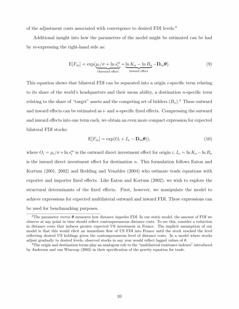
Additional insight into how the parameters of the model might be estimated can be had

by re-expressing the right-hand side as:

E[Fin] = exp(µi/σ + ln smi︸ ︷︷ ︸

Outward effect

+ ln Kn − ln Bn︸ ︷︷ ︸Inward effect

−Dinθ). (9)

This equation shows that bilateral FDI can be separated into a origin i-specific term relating

to its share of the world’s headquarters and their mean ability, a destination n-specific term

relating to the share of “target” assets and the competing set of bidders (Bn).4 These outward

and inward effects can be estimated as i- and n-specific fixed effects. Compressing the outward

and inward effects into one term each, we obtain an even more compact expression for expected

bilateral FDI stocks:

E[Fin] = exp(Oi + In −Dinθ)), (10)

where Oi = µi/σ+ln smi is the outward direct investment effect for origin i, In = ln Kn− ln Bn

is the inward direct investment effect for destination n. This formulation follows Eaton and

Kortum (2001, 2002) and Redding and Venables (2004) who estimate trade equations with

exporter and importer fixed effects. Like Eaton and Kortum (2002), we wish to explore the

structural determinants of the fixed effects. First, however, we manipulate the model to

achieve expressions for expected multilateral outward and inward FDI. These expressions can

be used for benchmarking purposes.

3The parameter vector θ measures how distance impedes FDI. In our static model, the amount of FDI weobserve at any point in time should reflect contemporaneous distance costs. To see this, consider a reductionin distance costs that induces greater expected US investment in France. The implicit assumption of ourmodel is that this would elicit an immediate flow of US FDI into France until the stock reached the levelreflecting desired US holdings given the contemporaneous level of distance costs. In a model where stocksadjust gradually to desired levels, observed stocks in any year would reflect lagged values of θ.

4The origin and destination terms play an analogous role to the “multilateral resistance indexes” introducedby Anderson and van Wincoop (2003) in their specification of the gravity equation for trade.

10

2.3 Implications for multilateral FDI

UNCTAD calculates its FDI Performance Index as the ratio of a country’s share of world FDI

to its share of world GDP. In this section, we aggregate bilateral FDI to derive predictions for

multilateral FDI in the context of our model. We show that even the simplest formulation of

the model—one with no distance costs—generates predictions of a country’s share of world

FDI that differ from the one used by UNCTAD.

Summing across bidders for a given destination country, we obtain expected worldwide

(w) foreign direct investment received by country n:

E[Fwn] =∑i6=n

E[Fin] = Kn

∑i6=n

πin = Kn(1− πnn). (11)

The summation across i 6= n arises because the “F” in FDI excludes investment by domes-

tic bidders in domestic targets (which equals πnnKn). Worldwide FDI stocks are found by

summing the national inward stocks:

E[Fw] =∑

n

E[Fwn] =∑

n

(Kn − πnnKn) = Kw −∑

n

πnnKn. (12)

The amount of total outward investment by country i is given by

E[Fiw] =∑n6=i

E[Fin] =∑n6=i

πinKn = Ki(Ai − πii), (13)

where Ai ≡∑

n πin(Kn/Ki). A comparison of multilateral inward and outward investment

for a given country i suggests an interpretation for the Ai term. Outward investment, Fiw,

equals inward investment, Fwi, if and only if Ai = 1. Thus, Ai is a measure of the “bidder

advantage” for country i when Ai > 1 and “bidder disadvantage” when Ai < 1.

The equations above result simply from adding up accounting identities. Equations (5)

and (8) imply that

πii = smi exp[µi/σ −Diiθ]B−1

i

11

is the domestically owned share of domestic assets. Letting sKi = Ki/Kw represent the share

of the world’s capital in country i, bidder advantage is given by

Ai = (smi /sK

i ) exp[µi/σ]∑

n

exp[−Dinθ]B−1n sK

n .

The inward FDI benchmark is given by the predicted value of i’s share of world inward FDI

stock:

f Ii =

E[Fwi]

E[Fw]= sK

i

1− πii

1− H,

where H =∑

n πnnsKn is the share of the world’s capital stock held by domestic controllers.

The outward FDI benchmark is given by the predicted value of i’s share of world outward

FDI stock:

fOi =

E[Fiw]

E[Fw]= sK

i

Ai − πii

1− H.

Consider the case of no distance costs, θ = 0, and that each country’s shares of bidders and

targets are proportional to its GDP share, smi = sK

i = si ≡ Yi/Yw. Then predicted outward

shares equal predicted inwards shares,

fOi = f I

n = si1− si

1−H, (14)

where H ≡∑

i s2i is the Herfindahl concentration index for the worldwide distribution of

GDP. It is interesting to compare this predicted FDI share, which we call the neutral bench-

mark, to the UNCTAD FDI Performance Index. Since UNCTAD scales FDI shares by GDP

shares, their implicit benchmark is si. The neutral benchmark therefore differs from the

UNCTAD benchmark because it adjusts for country size relative to the concentration index,

(1 − si)/(1 − H). FDI shares for small countries are predicted to be larger than their GDP

shares. Thus, other things equal, we expect relatively high UNCTAD performance indexes for

small countries. Since H = 0.14 in 2001, only the US (si = 0.32 in 2001) is large enough so

that its share of world FDI is predicted to be less than its share of world GDP. The neutral

benchmark predicts all other counties to have FDI shares greater than their GDP shares. In

12

2004 the UNCTAD reported that “The results show that relatively small economies such as

Switzerland feature prominently on the top of the list. This suggests that these economies

have highly competitive enterprises with ownership advantages that enable them to compete

successfully in international markets.”5 The size-bias inherent to the UNCTAD benchmark

raises doubts about this inference.

3 FDI and M&A

We fit our model to both FDI and M&A data. The source of the foreign direct investment

statistics used in this study is the Balance of Payments that reflects cross-border flows of

goods, services, and ownership claims. We obtain bilateral FDI from the Organization for Eco-

nomic Cooperation and Development’s (OECD) SourceOECD International Direct Investment

Statistics database. The original source of M&A data is Thomson Financial Securities Data

Corporation who compile information on all mergers and acquisitions that involve at least a

5% change in firm equity. Multilateral FDI and M&A data are available from UNCTAD’s

FDI database.6 Bilateral M&A transactions from 1990 to 1999 are kindly made available by

di Giovanni (julian.digiovanni.ca).

For a number of reasons, cross-border M&A transactions are not a proper subset of FDI

data. First, M&A data includes funds raised locally. For example, an acquisition by a foreign

enterprise resident in the country of the target is recorded in the M&A statistics but not in

the FDI statistics (since no cross-border flow of funds has occurred). Second, the M&A data

reflect gross transactions amounts at the time of the deal and do not account for subsequent

investment or divestitures. Third, the M&A values recorded at the time of the announcement

or closure of the deal may not correspond exactly to the flow of investment funds.7

Despite these definitional differences, it is useful to observe the relationship between the

two data series. We collected multilateral FDI flow and M&A data from UNCTAD’s Foreign

5www.geneva.ch/_FDI_performance.htm6The M&A data are based on the acquirer obtaining at least a 10% stake in the target company.7These definitional issues are discussed in the World Investment Report 2000, Chapter IV, pp.104–109.

13

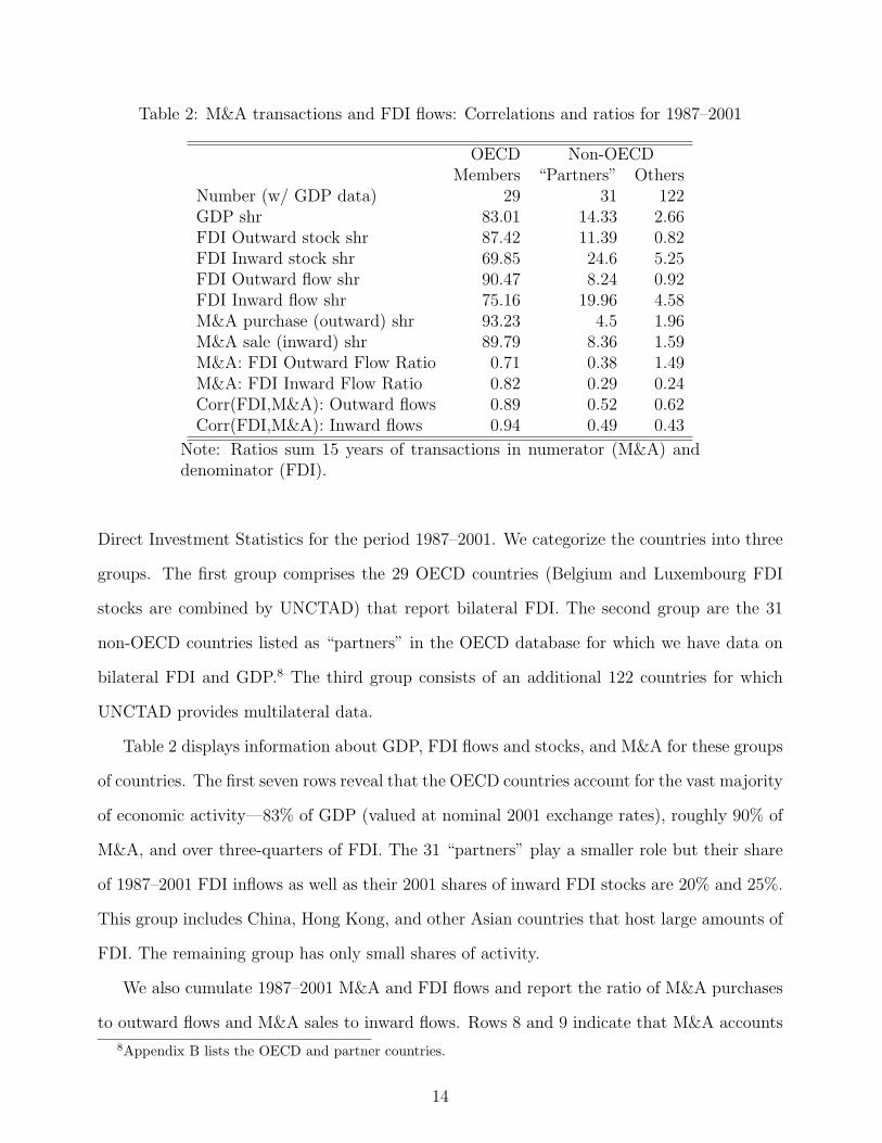
Table 2: M&A transactions and FDI flows: Correlations and ratios for 1987–2001

OECD Non-OECDMembers “Partners” Others

Number (w/ GDP data) 29 31 122GDP shr 83.01 14.33 2.66FDI Outward stock shr 87.42 11.39 0.82FDI Inward stock shr 69.85 24.6 5.25FDI Outward flow shr 90.47 8.24 0.92FDI Inward flow shr 75.16 19.96 4.58M&A purchase (outward) shr 93.23 4.5 1.96M&A sale (inward) shr 89.79 8.36 1.59M&A: FDI Outward Flow Ratio 0.71 0.38 1.49M&A: FDI Inward Flow Ratio 0.82 0.29 0.24Corr(FDI,M&A): Outward flows 0.89 0.52 0.62Corr(FDI,M&A): Inward flows 0.94 0.49 0.43

Note: Ratios sum 15 years of transactions in numerator (M&A) anddenominator (FDI).

Direct Investment Statistics for the period 1987–2001. We categorize the countries into three

groups. The first group comprises the 29 OECD countries (Belgium and Luxembourg FDI

stocks are combined by UNCTAD) that report bilateral FDI. The second group are the 31

non-OECD countries listed as “partners” in the OECD database for which we have data on

bilateral FDI and GDP.8 The third group consists of an additional 122 countries for which

UNCTAD provides multilateral data.

Table 2 displays information about GDP, FDI flows and stocks, and M&A for these groups

of countries. The first seven rows reveal that the OECD countries account for the vast majority

of economic activity—83% of GDP (valued at nominal 2001 exchange rates), roughly 90% of

M&A, and over three-quarters of FDI. The 31 “partners” play a smaller role but their share

of 1987–2001 FDI inflows as well as their 2001 shares of inward FDI stocks are 20% and 25%.

This group includes China, Hong Kong, and other Asian countries that host large amounts of

FDI. The remaining group has only small shares of activity.

We also cumulate 1987–2001 M&A and FDI flows and report the ratio of M&A purchases

to outward flows and M&A sales to inward flows. Rows 8 and 9 indicate that M&A accounts

8Appendix B lists the OECD and partner countries.

14

for a large majority of the 29 OECD countries’ investment, with M&A sales representing

82% of inward FDI and purchases of foreign assets through M&A accounting for 71% percent

of outward FDI. The ratios are lower for the other groups of countries. The 1.49 ratio of

purchases to outward FDI for the third group, the 122 countries with multilateral data only,

reflects large M&A purchases by Bermuda and Bahrain coupled with much smaller recorded

outward FDI flows. For all countries, the ratio of M&A sales to inward FDI and M&A

purchases to outward FDI are 0.68 and 0.69, and these data are the basis for our statement

in the introduction reporting that FDI accounts for roughly two-thirds of FDI.

The last two rows list the correlation between outward FDI and M&A purchases and

inward FDI and M&A sales for the groups for the 1987–2001 period.9 The correlation is quite

high for the OECD countries—0.94 for inward investment and 0.89 for outward investment.

The correlations are around 0.5 for the other groups.

We have learned that M&A seems to characterize much of the FDI of OECD countries.

Does M&A reflect the market for corporate control that we focus on in the model? Additional

information sheds light on this issue. Gugler, Mueller, Yurtoglu and Zulehner (2003) calculate

the share of international M&As that are horizontal, vertical, and conglomerate for the 1981–

1998 period. They define horizontal mergers as those occurring between companies classified

in the same four-digit industry. Vertical mergers are those for which the firms are in different

4-digit SICs and the two SICs have at least 10% of their sales/purchases with one another

(based on the 1992 US input-output table). Conglomerate mergers are all others. They find

that 54% of cross-border M&A mergers are conglomerate, 42% are horizontal, and only 4%

are vertical. Hijzen, Gorg, and Manchin (2005) examine a slightly later period, 1990–2001,

and calculate that 32% of mergers are horizontal.

Conglomerate mergers and a portion of horizontal mergers may be consistent with our

model of corporate control. Conglomerate mergers occur when the investor can add value

to the target’s operations. The motivation for such mergers is unlikely to cause a shift in

the acquirer’s production in order to lower costs, the traditional focus of FDI theory. Thus,

9We stack M&A and FDI data for each country and each year and compute correlations. Thus, correlationscontain both time series and cross-sectional variation.

15

we argue that these transactions are better modelled in our framework than one where trade

costs and factor costs play the central role. In addition, as demonstrated by the Renault-

Nissan example, some horizontal mergers are more related to adding value through better

management than lowering costs by shifting production.

While we have M&A in mind when developing the model, in light of this information on

M&A and FDI data, we feel our model can be applied to observed FDI levels. Most OECD

FDI is M&A and the costs and benefits of control are likely to be important considerations

for most M&A. Our model may also be able to represent greenfield investment in cases where

investors bid on a fixed number of investment sites and there is heterogeneity across investors

in the value they can add to the sites.

In the next section, we fit our model to 2001 bilateral FDI stocks and cumulative 1990–1999

M&A transaction values.

4 Bilateral FDI results

The recorded bilateral FDI data for 30 OECD countries and 32 non-OECD partners contains

both missing data and zero values. Once we cumulate 1990–1999 M&A data collected from di

Giovanni, we have 19,897 observations for 101 source countries and 198 destination countries.

Only 1551 of these observations, however, are non-zero and there are no missing values: di

Giovanni coded zeros for bilateral pairs with no M&A transactions. To keep the FDI and

M&A samples as consistent as possible, we confine the sample to the 30 OECD members and

the 32 additional “partners” listed in the OECD Direct Investment Statistics database.10

We estimate the model in two stages. In the first stage, we regress bilateral FDI stocks on

outward and inward fixed effects and a vector of geographic and cultural distance measures,

Dinθ. In the second stage, we regress the estimated outward and inward effects on variables

predicted by the model. Specifically, the outward effect is a function of the quality and quantity

of management teams (µi/σ +ln smi ) whereas the inward effect depends on a country’s capital

10We thereby discard 511 observations with positive M&A data. However, M&A levels for these observationsare quite small: only two exceed $10 billion with both of those involving Bermuda as the destination country.

16

stock (Kn) and bid competition (Bn).

To proceed, we need to move from the expected values determined in the theory section

to the actual values of FDI recorded in the OECD data set. Define ηin = Fin/E[Fin] as the

ratio of actual to expected bilateral FDI stocks. Using equation (10),

Fin = E[Fin]ηin = exp(Oi + In −Dinθ)ηin, (15)

Although ηin has an expected value of one, it can deviate from one for three main reasons.

First, in the context, of the model, lumpiness of the targets leads to variance in realized FDI

(see appendix A). Second, specification error is nearly unavoidable in a parsimonious model

based on particular functional forms. Third, governments measure FDI imperfectly.

The Din vector consists of log distance and adjustments based on observed and unobserved

bilateral linkages:

Din = {ln din, Langin, ToColyin FromColyin, uin},

where din is the average great circle distance between the 20 largest cities in countries i and n.11

Langin indicates that i and n share a common language. A prior colonial relationship is likely

to be a good proxy for institutional similarity that could facilitate monitoring. We introduce

directional dummy variables to indicate FDI to a former colony from its colonizer (ToColy)

and FDI from a colony to its colonizer (FromColy). The distance, language, and colony

variables are provided on the cepii.fr website. These variables have been found significant

in past studies of trade (e.g. Rose, 2004). We introduce uin to capture all the unobserved

linkages between two countries that affect the cost of monitoring. After introducing these

variables, the equation for bilateral FDI stocks becomes

Fin = exp[Oi + In − θ1 ln din + θ2Langin + θ3ToColyin + θ4FromColyin + (θ5uin + ln ηin)] (16)

11We experimented with dividing distance into six categories and using category dummy variables as inEaton and Kortum (2002) but found that the parsimonious linear-in-logs approach provides a slightly betterfit. The two distance decay functions are compared graphically in files available at http://strategy.sauder.ubc.ca/head/sup.

17

The conventional method for estimating (16) is to take logs of both sides, yielding

ln Fin = xinβ + εin, (17)

where xin is [1×K] vector of explanatory variables, xinβ ≡ Oi + In − θ1 ln din + θ2Langin +

θ3ToColyin + θ4FromColyin, and εin ≡ θ5uin + ln ηin. We can then estimate the parameters

(Oi, In, θ1–θ4) using linear regression. Since uin captures unobserved country-pair linkages,

we expect εin to be high correlated with the reverse direction error term εni. We therefore

estimate (17) using pair-wise random effects (GLS).

A well-known problem with estimating (17) is the log function eliminates all the zeros.

This problem is more severe for FDI and cross-border M&A than trade because of the much

higher frequency of bilateral zero stocks. Eaton and Tamura (1994) introduced Tobit-type

estimation methods for FDI and trade and Wei (2000) adopts the same method. Recent

simulations results of Santos Silva and Tenreyro (forthcoming) find that Eaton and Tamura’s

method can yield highly biased estimates in the presence of heteroskedastic errors. They point

out that if the variance of the error term ηin is a function of the covariates (such as ln din), then

the conditional expectation of ln ηin will not be zero and linear regression generates inconsistent

parameter estimates—regardless of whether the dependent variable contains zeros.

Santos Silva and Tenreyro argue that Poisson quasi-MLE is an attractive alternative to

least squares on equation (17). The K first order conditions for the Poisson QMLE are

∑i

∑n

(Fin − exp(xinβ))xkin = 0 for k = 1 . . . K , (18)

the same first order conditions used for Poisson MLE on count data. The Poisson QMLE

gives consistent β estimates no matter what the variance of ηin so long as E[Fin] = exp(xinβ).

Comparing with the least squares first order conditions,

∑i

∑n

(ln Fin − xinβ)xkin = 0 for k = 1 . . . K, (19)

18

we see that the former involves level deviations of Fin from its expected value whereas the

OLS involves log deviations. In comparing the fit of each model to the data, we therefore

report diagnostics (R2 and RMSE) in terms of both levels and logs. Another advantage of

Poisson QMLE is that it can incorporate the zero FDI stocks.12

Table 3: Bilateral FDI regressions with fixed effects: 2001

Specification: (1) (2) (3) (4) (5) (6)Method: GLS GLS GLS PQMLE PQMLE PQMLEDepvar: ln FDI ln FDI ln M&A FDI FDI M&ASample: All∗ Hi-OECD∗ All All Hi-OECD Allln distance -1.250a -1.048a -0.916a -0.591a -0.582a -0.726a

(0.072) (0.129) (0.095) (0.061) (0.083) (0.111)Language 0.697a 0.611b 1.147a 0.250c 0.215 0.593b

(0.191) (0.257) (0.233) (0.143) (0.163) (0.293)To colony 1.140a 0.831a 0.897a 0.201 0.096 0.125

(0.243) (0.314) (0.315) (0.198) (0.258) (0.286)From colony 0.772a 0.426 -0.171 0.328 0.262 0.687b

(0.274) (0.295) (0.452) (0.210) (0.242) (0.283)No. of obs. 1278 425 944 1559 453 2465R2 in logs 0.795 0.835 0.603 0.729 0.782 0.494R2 in levels 0.609 0.661 0.669 0.898 0.903 0.884RMSE in logs 1.466 1.215 1.765 1.795 1.481 2.094RMSE in levels 15.419 21.075 9.739 5.008 8.841 3.207

Note: GLS regressions estimated with country-pair random effects and heteroskedasticity-robuststandard errors. Poisson Quasi-MLE standard errors are robust to over/under dispersionand clustered at the country-pair level. Statistical significance at the 1%, 5% and 10% levelsparentheses denoted with a, b, and c. ∗ “All” comprises 30 OECD reporters and 32 partners.HI-OECD limits sample to 24 high-income countries (see data appendix).

Table 3 presents the coefficients on distance, common language, and colonial tie from

the first-stage regressions.13 The first three columns display the GLS results and the second

three columns Poisson QMLE results. Columns (1) presents GLS results for FDI stocks. In

common with gravity equations estimated for bilateral trade, distance impedes international

transactions while common language and colonial ties promote them. In this column, bilateral

FDI is higher for countries with colonial ties regardless of whether the source country is a

12Wooldridge (2002, Chapter 19) provides further detail on the robustness and efficiency properties ofPoisson QMLE for models with non-negative dependent variables even if they are continuous and do notfollow the Poisson variance assumption.

13We relegate the estimated outward and inward country fixed effects to Appendix B.

19

colonizer or former colony. Column (2) reflects FDI results when we confine the sample to

24 high-income OECD countries as both the source and destination countries (the Czech

Republic, Hungary, Mexico, Poland, Turkey, and Slovakia are excluded from the original

30 OECD countries). The logic of considering this sub-sample is that Table 2 indicates that

most FDI of these countries is M&A. The results do not change much with this smaller sample

except that the “From colony” variable loses statistical significance. Column (3) shows results

for cumulative M&A. Compared to the results for FDI shown in column (1), the estimates are

similar except that M&A from colonies is not estimated to have a statistically significantly

effect.

Turning to the Poisson QMLE estimates, we observe that this methods tends to produce

smaller coefficient estimates than corresponding GLS estimates. Santos Silva and Tenreyro

(forthcoming) find smaller distance and colony Poisson QMLE estimates than OLS estimates

in trade data.14 A negative distance effect is a common finding in the empirical FDI literature

and does not support the view of FDI serving as a means to avoid trade costs. Both our

GLS and our Poisson QMLE distance elasticities are larger than Wei (2000) and Eaton and

Tamura (1994), and Loungani, Mody, Razin and Sadka (2004) find for FDI and di Giovanni

and Hijzen, Gorg, and Manchin (2005) find for M&A.15 The estimates of the effect of com-

mon language are marginally significant for the full samples of countries in the FDI and M&A

regressions. However, common language enters insignificantly in the high-income OECD sam-

ple. The Poisson QMLE estimates of “From Colony” are larger than the “To Colony” across

specifications and samples, indicating that former colonies enjoy advantages when investing

in their colonizer.

Note that number of M&A observations in the Poisson QMLE regressions is much higher

than corresponding FDI regressions—2465 M&A observations versus 1559 FDI observations.

This is due to recorded zeros in the M&A regressions for observations where the OECD lists

FDI as missing (recall, di Giovanni generated zeros when no M&A was observed). We find that

14Their sample is 136 countries in 1990 and they do not divide colonial ties into its two components.15Wei, di Giovanni, and Loungani, Mody, Razin and Sadka include a variable measuring telephone linkages

between bilateral pairs that explain some of the distance effects we measure.

20

the Poisson results are remarkably robust to the treatment of zeros and missing values—they

hardly change when we turn zeros into “missings” and “missings” into zeros.

We use the full-sample as the basis for our second-stage estimations to maximize the

number of estimated outward and inward effects. We consider the Poisson QMLE results to

be the preferred specification for our second stage regressions. Appendix B lists the estimated

first-stage fixed effects used in the second stage regressions. The number of observations is

never the full 62 across specification due to missing data and other issues detailed in the

appendix.

The outward effect depends on country i’s share of world bidders and the quality of the

bidders, µi/σ. We assume the number of bidders, mi, is proportional to population, denoted

Ni, and that bidder quality can be represented by per capita GDP, denoted yi. Thus, the

outward fixed effect comprises scale (Ni) and development (yi) effects:

Oi = ln smi + µi/σ ∼ ω1 ln Ni + ω2 ln yi.

We estimate

Oi = C + ω1 ln Ni + ω2 ln yi + ei

where Oi is the estimated fixed effect from the first stage Poisson QMLE regression, C is a

constant, and ei is the second-stage error term. We match 2001 population and per-capita

income for FDI fixed effect regressions and 1999 population and per-capita income to the

M&A fixed effect regressions.16

The first two columns of Table 4 contain results for FDI and M&A. In both specifications,

the coefficient on ln Ni is insignificantly different from one, indicating that, after controlling for

the level of development, the number of bidders is proportional to the size of the population.

The strong effect of income per capita can be interpreted as capturing the average ability

effect embodied in the model as µi. We can also interpret the results as the number of bidders

being proportional to GDP, ln(Niyi). In that case, the coefficients on development become

16To correct for heteroscedasticity, we weight the observations by the inverse of the standard error from thefirst stage (see Saxonhouse, 1976).

21

Table 4: Second-stage regressions: 2001

Specification: (1) (2) (3) (4) (5)

Dep. var.: FDI Oi M&A Oi ln Kn FDI In M&A In

Scale (ln N) 1.009a 1.034a 1.022a 0.812a 1.10a

(0.078) (0.134) (0.030) (0.096) (0.133)Development (ln y) 2.158a 2.221a 0.964a 1.279a 1.630a

(0.109) (0.159) (0.035) (0.150) (0.204)Bid comp. (ln B) -0.510 -1.063b

(0.546) (0.505)N 61 51 132 60 56R2 0.879 0.804 0.933 0.681 0.666RMSE .896 1.249 .613 .971 1.242

Note: Weighted least squares regressions with a, b and c respectively denotingsignificance at the 1%, 5% and 10% levels.

1.149 and 1.187 in the FDI and M&A regressions. The two variables do a very good job of

predicting the outward fixed effect, achieving an R2 of 0.88 for outward FDI and 0.80 for M&A

transactions. These second stage results tell us that smi exp(µi/σ) is roughly proportional to

Niy2i .

To examine the determinants of the inward effect, In = ln Kn − ln Bn, we compute Bn =∑i N

ω1i yω2

i exp[Dinθ] using our measure of smi exp(µi/σ) and the θ estimates. Ideally, we

would regress the estimated inward effects on the host’s capital stock and Bn. Unfortunately,

capital stock data for 2001 are not available.17 Column (3) portrays results of regressing the

1990 capital stock data of Easterly and Levine (2002) for 132 countries on our scale, ln N ,

and development, ln y, variables. We observed that both are significant with elasticities close

to one and explain 93% of the variation in log capital stocks (ln K).18

We therefore use scale and development as proxies for capital and fit the following regres-

sion to our FDI and M&A inwards effects:

In = C + η1 ln Nn + η2 ln yn − ln Bn + en

17Data on stock market capitalization is also not available for all countries.18This data, based on the Penn World Tables 5.6, is available online at www.worldbank.org/research/

growth/pdfiles/GDN/Micro%20Time%20Series.xls.

22

The results are displayed in columns (4) and (5). Our theoretical model predicts that

the coefficients on the capital stock and bid competition will enter with unitary elasticity.

Thus, given the column (3) results, the proxies for capital stock, ln Nn and ln yn, should

obtain coefficients of 1.022 and .964. As can be observed, per capita income is entering more

strongly that what our theory predicts. A joint test of these restrictions along with unitary

elasticity for ln Bn is rejected at the 1% significance level.

Our parsimonious model posits no barriers to inward FDI other than monitoring costs as

proxied by distance, common language, and colonial ties. Of course, other country charac-

teristics will influence inward investment such as differences in institutions. Rossi and Volpin

(2001) use country institution data in La Porta et al. (1998) and find that the presence of

common law and high accounting standards and shareholder protection are associated with

greater M&A. We collected data on “rule of law” as reported by the World Bank for our

sample of countries and, in unreported regressions, add this variable to our inward effects

regressions. It enters positively with borderline significance in the FDI and M&A regressions

and lowers the coefficient on per capita income (the correlation between rule of law and per

capita GDP is 0.88). With the inclusion of this variable, we now are unable to reject the

unitary elasticity for the (proxied) capital stock and bid competition variables at the 10%

level.19

The results of the bilateral regressions provide support for the gravity specification for

FDI implied by our model of corporate control. Second-stage regressions using the estimated

outward effects show a strong effect of per capita income, highlighting the importance of source

country development for outward FDI. Investigation of the determinants of the inward effect

reveals that the proxies for capital shares enter with the expected unit elasticity. For reasons

outside the model, however, the level of development also exerts a positive influence on the

inward effect. This finding suggests that the inclusion of additional variables that describe the

19Similar second-stage findings emerge when we use GLS to estimate the first-stage equation. The coefficienton lnN in the outward effect regression is within one standard of one when we use FDI as the dependentvariable but is significantly below one in the M&A regressions (0.689, standard error 0.12). In the inwardestimates, lnB is within one standard deviation of -1 for the M&A regressions but is significantly less thanone (in absolute value) in the FDI regression (-0.268, standard error 0.19).

23

investment climate may capture variation in the inward effect beyond what is explained by

the model-based determinants. Our derivation shows that additional host-country variables

should be estimated via the two-step procedure outlined here.

5 Multilateral FDI results

In this section we show that our parsimonious, structural model conforms to the principal

patterns of aggregate FDI and M&A data. To do this, we apply the model and estimates

from the bilateral regressions to predict each country’s shares of world outward and inward

FDI in 2001 and cumulative 1987–2001 M&A flows.

Recall the specification on inward and outward shares:

f Ii =

E[Fwi]

E[Fw]= sK

i

1− πii

1− H.

fOi =

E[Fiw]

E[Fw]= sK

i

Ai − πii

1− H.

where πii = smi exp[µi/σ −Diiθ]B−1

i and

Ai = (smi /sK

i ) exp[µi/σ]∑

n

exp[−Dinθ]B−1n sK

n .

Since a country’s success at bidding for assets depends on its characteristics and geographic

location as well as those of all other countries, it is necessary to use information on all countries

in the world. We adhere to the theoretical structure of the model and use estimates of unknown

model parameters from the bilateral regression.20 We calculate each country’s quality adjusted

share of bidders as given by smi exp[µi/σ] ∼ Nω1

i yω2i where ω1 and ω2 are estimated coefficients

on ln N and ln y in the second-stage, outward effects regression. We calculate target assets

as Kn ∼ N1.02n y0.96

n , and distance from other countries as Dinθ. We compute Bn as described

20This means ignoring the additional effect of per capita GDP beyond the model prediction observed in thesecond stage regressions on the inward effect. Thus, deviations of actual inward FDI from our benchmark willreflect rule of law and other institutional differences across countries.

24

Table 5: Model performance: Mean absolute deviations of actual share (percentage points)minus predicted share.

Inward Outwardlevels logs levels logs

Full sample (172 Inward, 146 Outward)UNCTAD benchmark 0.364 0.749 0.508 2.533Neutral benchmark 0.311 0.727 0.466 2.630Estimated benchmark 0.315 0.785 0.425 1.774

High income OECD sample (23 countries)UNCTAD benchmark 1.914 0.703 2.270 0.729Neutral benchmark 1.536 0.658 1.884 0.690Estimated benchmark 1.376 0.620 2.242 0.585

previously.

We refer to our model predictions as the “estimated” benchmark which we compare to two

other benchmarks. The UNCTAD benchmark predicts FDI shares equalling GDP shares, si,

as implied by UNCTAD’s FDI Performance Index. The neutral benchmark assumes bidder

and target shares are proportional to GDP and there are no distance effects. As shown

earlier, in this case, FDI shares are related to GDP shares except that there is an adjustment

for relative country size.

Table 5 reports mean absolute deviations of the difference between each benchmark and

the actual shares for each country. We examine both level and log differences. In terms of

levels, the fit of the predictions to United States data dominates the results as the US is such

a dominant source and recipient of FDI, accounting for 22% of outward stocks and 21% of

inward stocks in 2001. The first two columns report results for inward stocks and the second

two columns for outward stocks. There are 172 countries with positive inward stocks and

146 countries with positive outward stocks. The second frame of Table 5 provides the same

statistics for the sub-sample of 23 high-income OECD countries (one Belgium-Luxembourg

observation).

The estimated benchmark outperforms the UNCTAD benchmark in seven out of the eight

25

measures. The lone exception for differences in logs of inward investment for all countries.

The neutral benchmark also fits actual data better than the UNCTAD benchmark. The

estimated benchmark provides a superior fit relative to the other two for outward investment,

particularly when we computed deviations in terms of differences in logs. This is because our

model conditions outward investment on the quality of bidders as measured by per capita

GDP. However, the estimated benchmark over-predicts the United States share of outward

investment—37% of world outward stocks as compared to actual outward shares of 22%. This

is a consequence of the high US share of world GDP, 32%, and the importance that the

estimated benchmark ascribes to high per capita income (bidder quality).

Figures 1 and 2 plot the actual inward and outward FDI against the estimated benchmark

for the largest 50 countries in terms of 2001 GDP on a logarithmic scale. We identify countries

with their three digit ISO codes and indicate OECD countries with solid black circles. If the

estimated predictions were correct, all the points would line up on the 45-degree line. The

figures reveal the fit of the model to multilateral data and identify outliers. Overall, the

predictions are randomly dispersed around the 45 degree line—the slope of a regression line

of actual on predicted FDI is not significantly different from one for all countries as well as

the 50 shown in the figures. The “unbiasedness” of the estimated benchmark contrasts with

the UNCTAD and neutral benchmarks where the slope of the line of log actual outward share

on log predicted share exceeds 1.5 for the full sample. Unlike our benchmark, these other

benchmarks systematically over-predict outward FDI for poor countries.

With regard to inward investment, Japan, India, and Iran under perform relative to the

benchmark whereas Hong Kong, Singapore, Ireland, Belgium-Luxembourg, and the Nether-

lands over-perform.21 For outward investment, Figure 2 shows the data points well dispersed

around the 45-degree line with the largest (log) deviations exhibited by small countries.

Figures 3 and 4 relate the estimated predictions to cumulated 1987–2001 M&A from

Thompson for the 50 largest countries according to 1999 GDP.22 Again, the points are scat-

21Head and Ries (2005) provide analysis of Japan’s FDI performance over time.22We create the benchmarks using parameter estimates from cumulative 1900–1999 bilateral M&A and 1999

population and GDP.

26

●

●

●

●

●

●

●

●

●

●

●

●

●

●

●

●

●

●

●

●

●

●

●

●

●

●

●

●

●●

●

●

●

●

●

●

●●

●● ●

●

●

●

●

●

●

●

●●

Benchmark (estimate) share

Act

ual s

hare

1 10

0.1

110

ARE

ARG

AUS

AUT

BLX

BRA

CAN

CHECHL

CHN

COL

CZE

DEU

DNK

DZA

EGY

ESP

FIN

FRA

GBR

GRC

HKG

IDN

IND

IRL

IRN

ISR

ITA

JPNKOR

MEX

MYS

NLD

NOR

NZL

PAK

PERPHL

POLPRT RUS

SAU

SGPSWE

THA

TUR

TWN

USA

VENZAF

●

●

● ●

●

●

●

●

●

●

●

●

●

●

●●

●

●

●

●

●

●

Figure 1: Inward FDI Model Performance, Largest 50 Countries

●

●

●

●

●

●

●●

●

●

●

●

●

●

●

●

●

●

●

●

●

●

● ●

●

●

●

●

●

●

●

●

●

●

●

● ●●

●

●

●

●

●

●

●

●

●

●

●

●

Benchmark (estimate) share

Act

ual s

hare

0.01 0.1 1 10

0.01

0.1

110

ARE

ARG

AUS

AUT

BLX

BRA

CAN

CHE

CHL

CHN

COL

CZE

DEU

DNK

DZA

EGY

ESP

FIN

FRA

GBR

GRC

HKG

IDN IND

IRL

IRN

ISR

ITA

JPN

KOR

MEX

MYS

NLD

NOR

NZL

PAK PERPHL

POL

PRTRUS

SAU

SGPSWE

THA

TUR

TWN

USA

VEN

ZAF

●

●

●

●●

●

●

●

●

●

●

●

●

●

●

●

●

●

●

●

●

●

Figure 2: Outward FDI Performance, Largest 50 Countries

27

●

●

●

●

● ●

●

●

●●

●

●

●

●

●

●

●

●

●

●

●

●●

●

●

●

●●

●

●

●

●

●

●●

●

●

●

●

●

●

●

●

●

●

●

●

●

●

●

Estimated benchmark (percent share)

Act

ual s

hare

1 10

0.01

0.1

110

ARE

ARG

AUS

AUT

BLX BRA

CAN

CHECHL

CHNCOL

CZE

DEU

DNK

EGY

ESPFIN

FRA

GBR

GRC

HKG

HUN IDN

IND

IRL

ISR

ITAJPN

KORMEX

MYS

NGA

NLD

NORNZL

PAK

PER

PHL

POL

PRTRUS

SAU

SGP

SWE

THA

TUR

TWN

USA

VEN

ZAF

●

●

●

●

●

●

●

●

●

●

●

●

●

●●

●

●

●●

●

●

●

Figure 3: Inward (Sales) M&A Model Performance, Largest 50 Countries

●

●

●

●

●

●

●●

●●

●●

●

●

●

●

●

●

●

●

●

●●

●

●

●

●●

●

●●

●

●

●●

●

●●

●

●●

●

●

●

●

●

●

●

●

●

Estimated benchmark (percent share)

Act

ual s

hare

0.01 0.1 1 10

0.01

0.1

110

ARE

ARG

AUS

AUT

BLX

BRA

CAN

CHE

CHLCHN

COLCZE

DEU

DNK

EGY

ESP

FIN

FRAGBR

GRC

HKG

HUNIDNIND

IRL

ISR

ITAJPN

KOR

MEXMYS

NGA

NLD

NORNZL

PAK

PERPHL

POL

PRTRUSSAU

SGP

SWE

THA

TUR

TWN

USA

VEN

ZAF

●

●

●

●●

●

●

●

●

●

●

●

●

●●

●

●

●●

●

●

●

Figure 4: Outward (Purchases) M&A Performance, Largest 50 Countries

28

tered randomly around the 45-degree line, with the slope of line relating actual shares to

predicted shares being insignificantly different from one (1.07 for inward M&A and 0.90 for

outward M&A). The pictures identify Saudi Arabia, India and China as selling fewer assets

than predicted. Among OECD countries, Great Britain and the Netherlands purchase more

assets than predicted while Japan and the United States purchase too few.

6 Conclusion

We develop a model explaining foreign direct investment based on an international market

for corporate control. After controlling for geographic and cultural distance effects between

bilateral partners, FDI depends on origin-country effects (outward effects) and destination-

country effects (inward effects). The latter includes a “bid competition” term that reflects

characteristics of competing countries. Our model highlights the importance of taking into

account the influence of third-country effects in bilateral estimation, thus echoing the insight

of Anderson and van Wincoop (2003) for the application of the gravity equation to bilateral

trade.

We use bilateral FDI data for 30 OECD countries and 32 partner countries to estimate

the unknown parameters and test predictions of the model. We find that proxies for coun-

tries’ shares of bidders and targets enter as predicted. Moreover, we find that the level of

development of the source country exerts a strong, positive influence on outward FDI.

Applying our model and estimates from bilateral regressions, we calculate predicted inward

and outward shares of world FDI for all countries in 2001 and compare them to actual values.

We find that the model fits the data fairly well. Indeed, the good fit even for countries where

M&A is relatively unimportant suggests that an analytical derivation of a gravity equation

for greenfield investment with frictions would be a helpful complement to this model.

Our empirical model of bilateral FDI intentionally uses a very small number of explanatory

variables that we can incorporate within a structural model. We do this partly to investigate

how well a parsimonious model can account for the global pattern of FDI and also to facilitate

29

calculation of the multilateral benchmarks for the largest set of countries and periods. One

can use the structural model as a baseline to identify deviations and then introduce additional

covariates to improve the fit or evaluate the impact of policies on FDI.

References

Anderson, J.E., van Wincoop, E., 2003, “Gravity With Gravitas: A Solution to the BorderPuzzle”, American Economic Review, 93(1): 170-192.

Anderson, S., De Palma, A. Thisse, J-F. (1992), Discrete Choice Theory of Product Differ-entiation (MIT Press, Cambridge).

Axtell, R.L., 2001, “Zipf Distribution of U.S. Firm Sizes,” Science 293, 1818-1820.

Barba Navaretti, G. Venables, A.J. 2004, Multinational firms in the world economy, PrincetonUniversity Press, New Jersey.

Benassy-Quere A., M. Coupet, and T. Mayer, 2007, “Institutional Determinants of ForeignDirect Investment”, World Economy.

Bergstrand, J.H., Egger, P., 2004, “A Knowledge-and-Physical-Capital Model of Interna-tional Trade, Foreign Direct Investment, and Outsourcing: Part I, Developed Coun-tries,” Notre Dame University manuscript.

Carr, D., Markusen, J.R., Maskus, K.E., 2001, “Estimating the Knowledge-Capital Modelof the Multinational Enterprise.” American Economic Review 91(3), 693–708.

Bury, K., 1999, Statistical Distributions in Engineering, Cambridge University Press.

di Giovanni, J., 2005, ”What Drives Capital Flows? The Case of Cross-Border M&A Activityand Financial Deepening,” Journal of International Economics 65, 127–149.

Grossman, G.M., Helpman, E., Szeidl, A., 2003, “Optimal Integration Strategies for theMultinational Firm” NBER Working Paper No. 10189.

Eaton, J., Kortum, S., 2002, “Technology, Geography, and Trade,” Econometrica 70(5),1741–1779.

Eaton, J., Kortum, S., 2001, “Trade in Capital Goods,” European Economic Review 45,1195–1235.

Eaton, J., Tamura, A., 1994, Bilateralism and Regionalism in Japanese and U.S. Trade andDirect Foreign Investment Patterns. J. Japanese Int. Economies 8, 478-510.

Eichengreen, B., Tong, H., 2005, “Is China’s FDI Coming at the Expense of Other Coun-tries?,” UC Berkeley manuscript.

30

Easterly, W., Levine, R., 2002, “It’s Not Factor Accumulation: Stylized Facts and GrowthModels” The World Bank Economic Review, VOL. 15, NO. 2, 177-219.

Fudenberg, D., Tirole, J. 1991, Game Theory, Boston: MIT Press.

Gordon, R.H., Bovenberg, A.L., 1996, “Why is capital so immobile internationally? Possibleexplanations and implications for capital income taxation” American Economic Review86(5), 1057-1075.

Gugler, K., Mueller, D.C., Yurtoglu, B.B., Zulehner, C., 2003, “The Effects of Mergers: AnInternational Comparison”, International Journal of Industrial Organization, 21, pp.625–653.

Head, K., Ries, J., 2005, “Judging Japan’s FDI: The verdict from a dartboard model,”Journal of the Japanese and International Economies 19, 215–232.

Helpman, E., 1984, A Simple Theory of Trade with Multinational Corporations. J. Polit.Economy 92, 451–471.

Hijzen, A., Gorg, H., Manchin, M., 2005, “Cross-Border Mergers and Acquisitions and theRole of Trade Costs,” manuscript.

Jensen, M.C., Ruback, R.S., 1983, The market for corporate control: The scientific evidence.J. Finan. Econ. 11, 5-50.

La Porta, R., Lopez-de-Silanes, F., Shleifer, A., Vishny, R., 1998, “Law and finance,” Journalof Political Economy 101, 678-709.

Loungani, P., Mody, A., Razin, A., Sadka, E., 2003, “The Role of Information in DrivingFDI: Theory and Evidence,” Scottish Journal of Political Economy 49, pp.546-543.

Marin, D., Schnitzer, M., 2004, “Global versus Local: The Financing of Foreign DirectInvestment,” University of Munich, Department of Economics, manuscript

Markusen, J., 1984, Multinationals, Multi-Plant Economies, and the Gains from Trade. J.Int. Econ. 16, 205-226.

Martin, P., Rey, H., 2004, “Financial super-markets: size matters for asset trade,” Journalof International Economics 64, 335-361.

Mody, A., Razin, A., Sadka, E., 2004, “The Role of Information in Driving FDI Flows: Host-Country Transparency and Source Country Specialization,” NBER Working Paper 9662.

Mutti, J., Grubert, H., 2004, “Empirical Asymmetries in Foreign Direct Investment andTaxation,” Journal of International Economics 62, 337–358.

Naldi, M., 2003, “Concentration indices and Zipf’s law,” Economics Letters 78, 329–334.

Neary, J.P., 2004, “Cross-Border Mergers as Instruments of Comparative Advantage,” Uni-versity College Dublin manuscript.

31

Nocke, V., Yeaple, S. 2005a, “Mergers and the Composition of International Commerce,”University of Pennsylvania manuscript.

Nocke, V., Yeaple, S., 2005b, “An Assignment Theory of Foreign Direct Investment,” NBERWorking paper 11003.

Organization for Economic Cooperation and Development (OECD), 2002, SourceOECD In-ternational Direct Investment Statistics database, www.oecd.org

Portes, R., Rey, H., 2005, “The Determinants of Cross-Border Equity Flows,” Journal ofInternational Economics 65, 269-296.

Razin, A., Sadka, E., Yuen, C-W. 1998, “A pecking order of capital inflows and internationaltax principles” Journal of International Economics 44, 45-68.

Razin, A., Goldstein, I., 2005, “An information-based trade off between foreign direct invest-ment and foreign portfolio investment,” NBER Working Paper 11757.

Redding, S., Venables, A.J., 2004, “Economic geography and international inequality,” Jour-nal of International Economics 62(1), 53-82.

Rose, A.K., 2004, “Do We Really Know that the WTO Increases Trade?,” American Eco-nomic Review 94(1), 98–114.

Rossi, S., Volpin, P., 2003, “CrossCountry Determinants of Mergers and Acquisitions,” Lon-don Business School manuscript.

Saxonhouse, G.R., 1976, Estimated Parameters as Dependent Variables, American EconomicReview 66(1), 178-183.

Santos Silva, J.M.C. Tenreyro, S., “The Log of Gravity,” Review of Economics and Statistics,forthcoming.

United Nations Conference on Trade and Development (UNCTAD), 2000, World InvestmentReport 2000: Cross-border Mergers and Acquisitions and Development, New York.

United Nations Conference on Trade and Development (UNCTAD), 2000, FDI Datadase,stats.unctad.org/fdi.

Wei, S-J., 2000, “How Taxing is Corruption on International Investors,” Review of Economicsand Statistics 1, 1–11.

Wooldridge, J.M., 2002, Econometric Analysis of Cross Section and Panel Data, MIT Press:Cambridge.

32

Appendix A: Variance in FDI due to lumpiness

Suppressing the in country subscripts, let subscript τ indicate a particular target in country n.

Let zτ be a binary variable that takes the value of 1 if a headquarters from i has acquired target

τ and zero otherwise. The expectation of z is the probability of it being equal to one: E[zτ ] = π.

The actual share of foreign-owned assets can then be expressed as F/K =∑T

τ zτKτ , where

there are T targets and Kτ is the size of target τ and K =∑T

τ Kτ . The expected value of

F/K is π. The variance of F/K is given by

Var

(∑Tτ zτKτ

K

)=

T∑τ

Var[zτ (Kτ/K)] = π(1− π)T∑τ

(Kτ/K)2 = π(1− π)H,

where H is called the Herfindahl concentration index for capital. Thus, FDI variance is

increasing in the concentration of capital in the destination country. If all firms were the

same size, Kτ = k, then H = 1/T and the variance of F/K goes to zero as the number of

firms, T , becomes large. Actual firm size distributions are highly skewed. Axtell (2001) finds

that the US firm size distribution is Pareto with a shape parameter near one (Zipf’s Law).

Equation (10) of Naldi (2003) shows that these assumptions imply

H =

∑Tτ=1 τ−2

(∑T

τ=1 τ−1)2.

Evaluating this expression we find that H = 0.06 for T = 100, H = 0.03 for T = 1000, and

H = 0.02 for T = 5000. Because the firm size distribution is highly skewed, Fin/Kn does not

converge quickly on πin and therefore “lumpiness” would appear to be an important source

of variance in FDI stocks.

Appendix B: Data

SourceOECD International Direct Investment Statistics database contains data on FDI inward

and outward positions. We use these data to compile as complete a file of bilateral FDI stocks

in 2001 as possible. We mainly use source-country reports to measure the stock of FDI of

country i into country n. When country i does not report a positive stock and the inward

stock reported by n is positive, then we use this inward stock instead.

Table 6 lists the 62 countries that constitute the bilateral data set. We list the inward

and outward effects estimated in the first-stage FDI and M&A regressions (US normalized

to 0). Netherlands Antilles has missing GDP data so the number of observations for second-

stage regressions, shown in Table 4, never equals 62. The 51 outward M&A observations

are a result of no M&A data for Algeria, Netherlands Antilles, Kuwait, Libya, Luxembourg,

33

and Taiwan plus our decision to drop the five countries for which we estimated fixed effects

even though all bilateral M&A purchases were recorded as zero—United Arab Emirates, Iran,

Slovenia, Iceland, and Cost Rica. We do not report the estimated fixed effects for these

latter countries but they are much larger in absolute value than those for countries with some

positive FDI purchases (estimates of less than -25). When we include these five countries,

the standard error increases dramatically. Kuwait had only zero levels of bilateral inward

FDI and we exclude it in the second-stage inward FDI regression. Inward M&A regressions

have 56 observations because of missing GDP data for Netherlands Antilles, no M&A data

for Kuwait, Luxembourg, and Taiwan and dropping Libya and Iran because they received no

inward FDI.

34

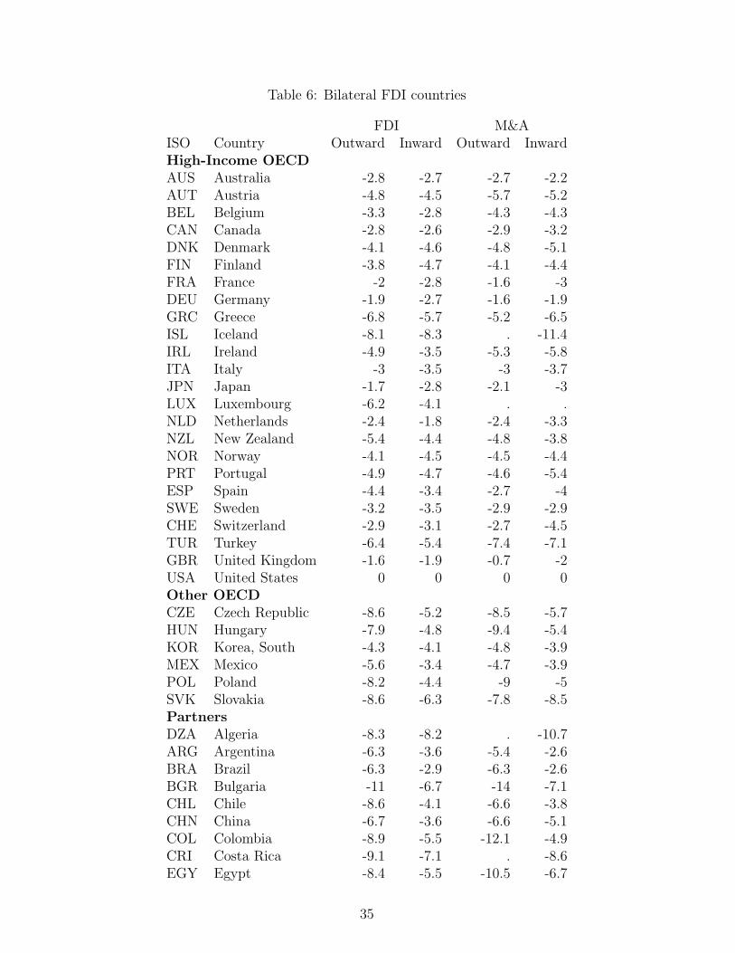
Table 6: Bilateral FDI countries

FDI M&AISO Country Outward Inward Outward InwardHigh-Income OECDAUS Australia -2.8 -2.7 -2.7 -2.2AUT Austria -4.8 -4.5 -5.7 -5.2BEL Belgium -3.3 -2.8 -4.3 -4.3CAN Canada -2.8 -2.6 -2.9 -3.2DNK Denmark -4.1 -4.6 -4.8 -5.1FIN Finland -3.8 -4.7 -4.1 -4.4FRA France -2 -2.8 -1.6 -3DEU Germany -1.9 -2.7 -1.6 -1.9GRC Greece -6.8 -5.7 -5.2 -6.5ISL Iceland -8.1 -8.3 . -11.4IRL Ireland -4.9 -3.5 -5.3 -5.8ITA Italy -3 -3.5 -3 -3.7JPN Japan -1.7 -2.8 -2.1 -3LUX Luxembourg -6.2 -4.1 . .NLD Netherlands -2.4 -1.8 -2.4 -3.3NZL New Zealand -5.4 -4.4 -4.8 -3.8NOR Norway -4.1 -4.5 -4.5 -4.4PRT Portugal -4.9 -4.7 -4.6 -5.4ESP Spain -4.4 -3.4 -2.7 -4SWE Sweden -3.2 -3.5 -2.9 -2.9CHE Switzerland -2.9 -3.1 -2.7 -4.5TUR Turkey -6.4 -5.4 -7.4 -7.1GBR United Kingdom -1.6 -1.9 -0.7 -2USA United States 0 0 0 0Other OECDCZE Czech Republic -8.6 -5.2 -8.5 -5.7HUN Hungary -7.9 -4.8 -9.4 -5.4KOR Korea, South -4.3 -4.1 -4.8 -3.9MEX Mexico -5.6 -3.4 -4.7 -3.9POL Poland -8.2 -4.4 -9 -5SVK Slovakia -8.6 -6.3 -7.8 -8.5PartnersDZA Algeria -8.3 -8.2 . -10.7ARG Argentina -6.3 -3.6 -5.4 -2.6BRA Brazil -6.3 -2.9 -6.3 -2.6BGR Bulgaria -11 -6.7 -14 -7.1CHL Chile -8.6 -4.1 -6.6 -3.8CHN China -6.7 -3.6 -6.6 -5.1COL Colombia -8.9 -5.5 -12.1 -4.9CRI Costa Rica -9.1 -7.1 . -8.6EGY Egypt -8.4 -5.5 -10.5 -6.7

35

FDI M&AISO Country Outward Inward Outward InwardPartners (cont’d)HKG Hong Kong -4.7 -3.3 -3.8 -4.2IND India -7.4 -5.1 -8.1 -6.1IDN Indonesia -7.4 -4 -5.5 -4.5IRN Iran -5.9 -7.2 . .ISR Israel -5.7 -5.4 -5.6 -5.1KWT Kuwait -4.3 . . .LBY Libya -8.7 -8 . .MYS Malaysia -5.1 -4.2 -3.7 -5.5MAR Morocco -7.9 -6.4 -9.5 -7.4ANT Netherlands Antilles -3.9 -4.6 . -7.9PAN Panama -6.5 -6 -11.5 -6.7PHL Philippines -9.3 -4.9 -9.5 -4.9ROM Romania -9.6 -6.3 -11.8 -6.4RUS Russian Federation -5.4 -5.3 -7.3 -6.1SAU Saudi Arabia -6.4 -5.9 -4.8 -9.6SGP Singapore -4.4 -2.9 -4.2 -5SVN Slovenia -8.7 -7 . -9.3ZAF South Africa -5.7 -4.7 -3.7 -4.7TWN Taiwan -5.5 -4.4 . .THA Thailand -8.3 -4.3 -7.2 -5UKR Ukraine -10.4 -7.3 -10.4 -8.8ARE United Arab Emirates -6.1 -6.3 . -8.6VEN Venezuela -5.8 -4.7 -6.1 -5

36